TRANSPORT AND MIXING ENHANCEMENT IN FLUID-THERMAL...

UNIVERSIDAD POLITÉCNICA DE MADRID

ESCUELA TÉCNICA SUPERIOR DE INGENIEROS

AERONÁUTICOS

TRANSPORT AND MIXING

ENHANCEMENT IN

FLUID-THERMAL MICROSYSTEMS

DOCTORAL THESIS

By:

Miguel Reyes Mata

Ingeniero Aeronáutico

Mentored by:

Ángel Velázquez López Juan Ramón Arias Pérez

Doctor Ingeniero Industrial Doctor Ingeniero Aeronáutico

2013

ii

Acknowledgements

First and foremost, this thesis would not have been possible without theunqualified and relentless support of my advisors Professor Ángel VelázquezLópez and Professor Juan Ramón Arias Pérez. I am also indebted to mycolleagues, specially Diego Alonso Fernández, Elliott Bache, Sergio de LucasBodas, Marcos Antonio Rodríguez Jiménez and Unai Iradier Gutiérrez, fortheir support, assistance and friendship. Finally, I would like to give thanksto my parents, Miguel and Adi, my sister Rocio, and my girlfriend Pilar fortheir understanding, endless patience and encouragement when it was mostrequired.

iii

iv ACKNOWLEDGEMENTS

Abstract

In this thesis, experimental research focused on passive scalar transport isperformed in micro-systems with marked sense of industrial application, us-ing innovative methods in order to obtain better performances optimizingcritical design parameters or finding new utilities. Part of the results ob-tained in these experiments have been published into high impact factorjournals belonged to the first quarter of the Journal Citation Reports (JCR).

First of all the effect of tip clearance in a micro-channel based heat sink isanalyzed. Leaving a gap between channels and top cover, letting the channelscommunicate each other causes three-dimensional effects which improve theheat transfer between fluid and heat sink and also reducing the pressuredrop caused by the fluid passing through the micro-channels which has agreat impact on the total cooling pumping power needed.

It is also analyzed the enhancement produced in terms of dissipated heatin a micro-processor cooling system by improving the predominantly used finplate with a vapour chamber based heat spreader which contains a two-phasefluid inside. It has also been developed at the same time a numerical modelto optimize the new fin plate dimensions compatible with a series of designrequirements in which both size and wight plays a very restrictive role.

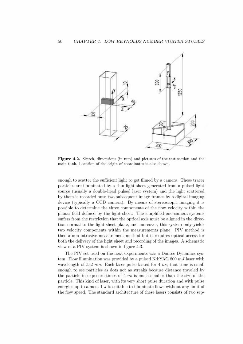
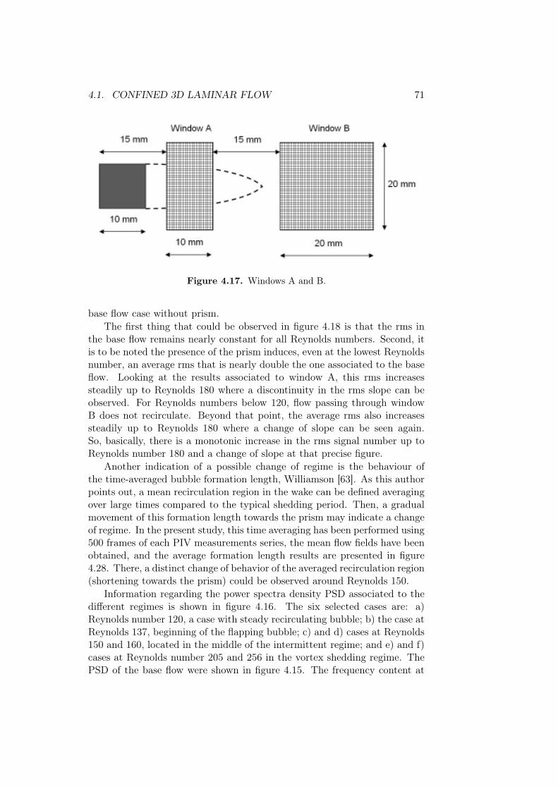
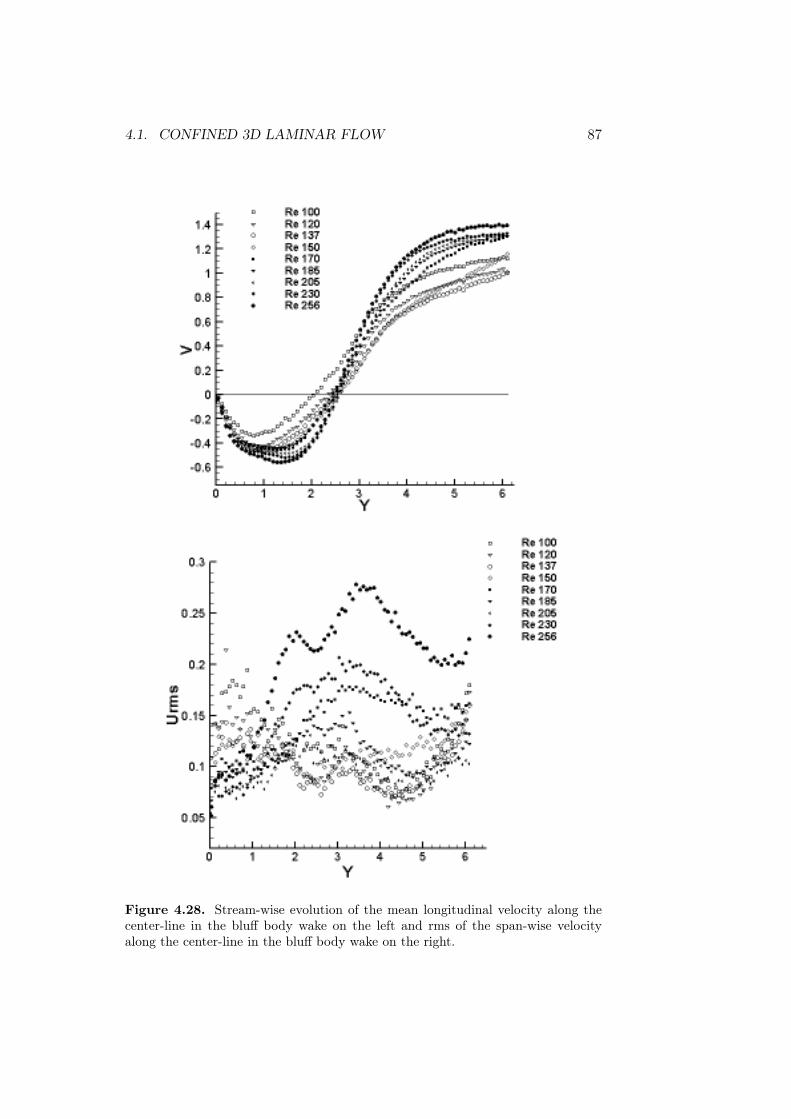
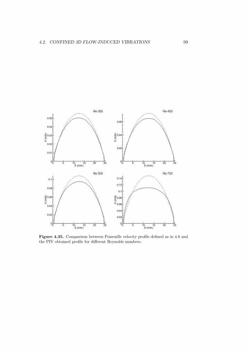
On the other hand, fluid-dynamics phenomena that appears downstreamof a bluff body in the bosom of a fluid flow with high blockage ratio hasbeen studied. This research experimentally confirms the existence of an in-termediate regime characterized by an oscillating closed recirculation bubbleintermediate regime between the steady closed recirculation bubble regimeand the vortex shedding regime (Karman street like regime) as a functionof the incoming flow Reynolds number. A particle image velocimetry tech-nique (PIV) has been used in order to obtain, analyze and post-process thefluid-dynamic data.

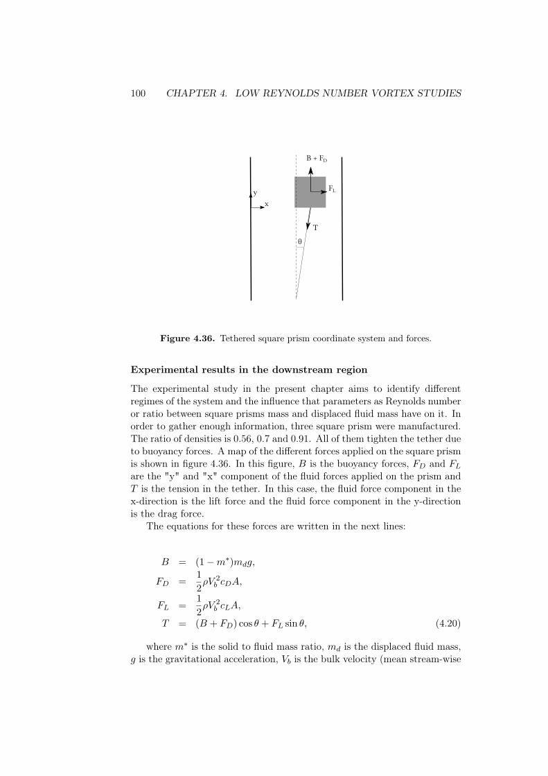
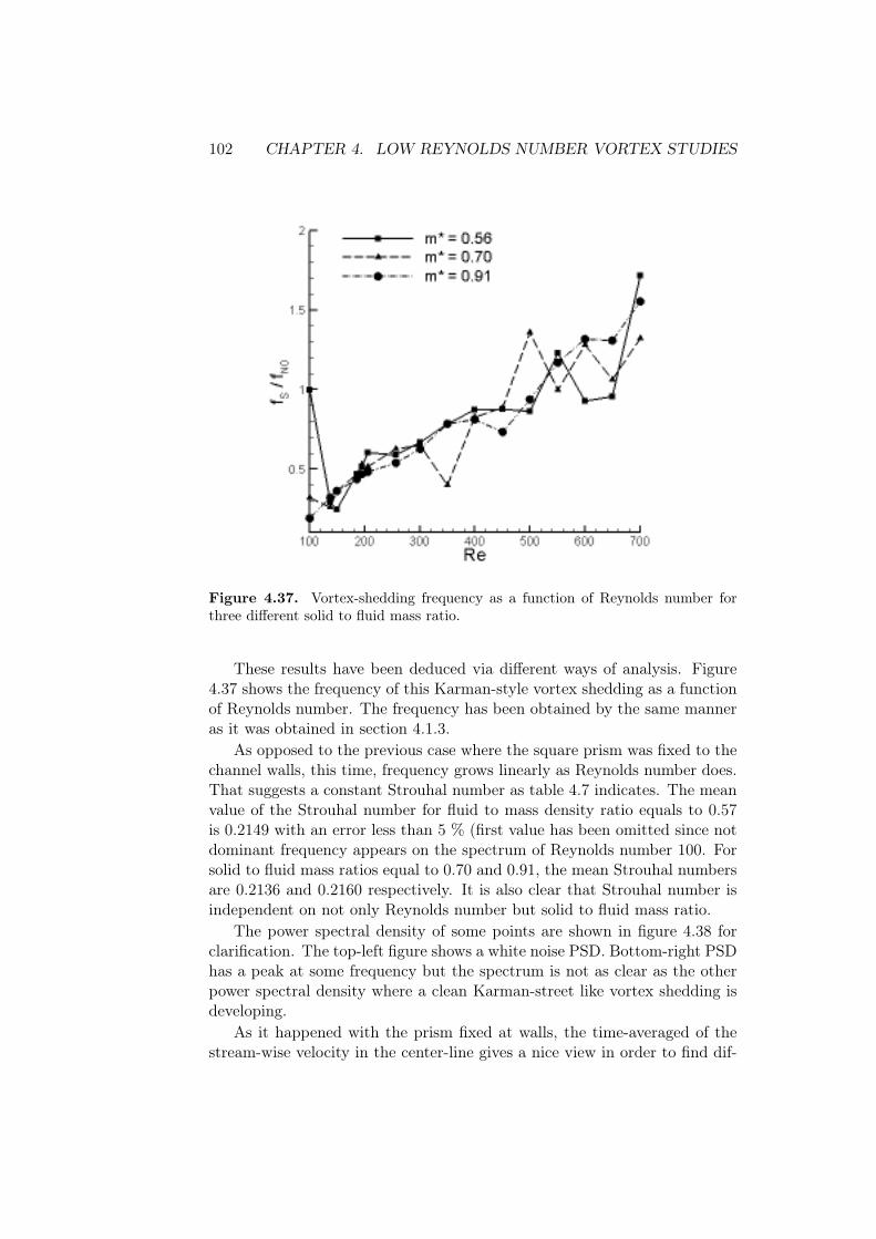
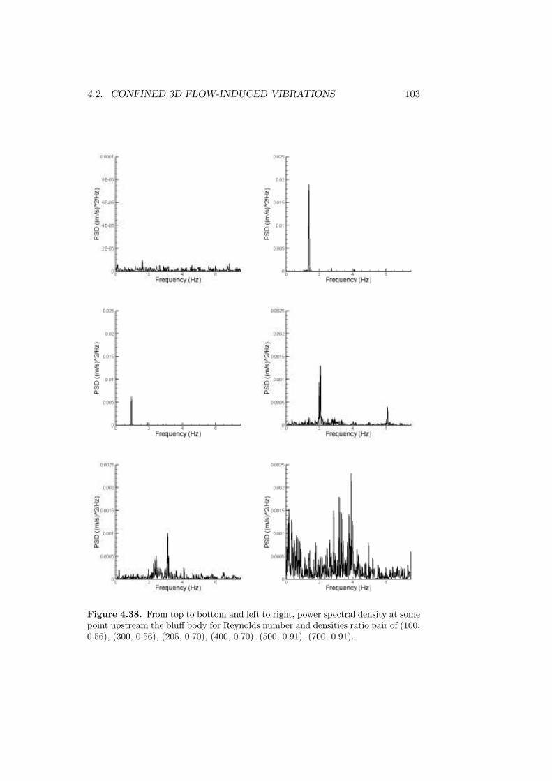
Finally and as an addition to the last point, a study on the vortex-induced vibrations (VIV) of a bluff body inside a high blockage ratio channelhas been carried out taking advantage of the results obtained with the fixedsquare prism. The prism moves with simple harmonic motion for a Reynoldsnumber interval and this movement becomes vibrational around its axial axisafter overcoming at definite Reynolds number. Regarding the fluid, vortexshedding regime is reached at Reynolds numbers lower than the previous

v

vi ABSTRACT

critical ones. Merging both movement spectra and varying the square prismto fluid mass ratio, a map with different global states is reached. This isnot only applicable as a mixing enhancement technique but as an energyharvesting method.

Resumen

En esta tesis se investiga de forma experimental el transporte pasivo de mag-nitudes físicas en micro-sistemas con carácter de inmediata aplicación indus-trial, usando métodos innovadores para mejorar la eficiencia de los mismosoptimizando parámetros críticos del diseño o encontrar nuevos destinos deposible aplicación. Parte de los resultados obtenidos en estos experimentoshan sido publicados en revistas con un índice de impacto tal que pertenecenal primer cuarto del JCR.

Primero de todo se ha analizado el efecto que produce en un intercam-biador de calor basado en micro-canales el hecho de dejar un espacio entrecanales y tapa superior para la interconexión de los mismos. Esto generaefectos tridimensionales que mejoran la exracción de calor del intercambi-ador y reducen la caída de presión que aparece por el transcurso del fluido através de los micro-canales, lo que tiene un gran impacto en la potencia queha de suministrar la bomba de refrigerante.

Se ha analizado también la mejora producida en términos de calor disi-pado de un micro-procesador refrigerado con un ampliamente usado platode aletas al implementar en éste una cámara de vapor que almacena un flu-ido bifásico. Se ha desarrollado de forma paralela un modelo numérico paraoptimizar las nuevas dimensiones del plato de aletas modificado compatiblescon una serie de requerimientos de diseño en el que tanto las dimensionescomo el peso juegan un papel esencial.

Por otro lado, se han estudiado los fenomenos fluido-dinámicos que apare-cen aguas abajo de un cuerpo romo en el seno de un fluido fluyendo por uncanal con una alta relación de bloqueo. Los resultados de este estudio con-firman, de forma experimental, la existencia de un régimen intermedio, car-acterizado por el desarrollo de una burbuja de recirculación oscilante entrelos regímenes, bien diferenciados, de burbuja de recirculación estacionaria ycalle de torbellinos de Karman, como función del número de Reynolds delflujo incidente. Para la obtención, análisis y post-proceso de los datos, seha contado con la ayuda de un sistema de Velocimetría por Imágenes dePartículas (PIV).

Finalmente y como adición a este último punto, se ha estudiado las vibra-ciones de un cuerpo romo producidas por el desprendimiento de torbellinosen un canal de alta relación de bloqueo con la base obtenida del estudio

vii

viii RESUMEN

anterior. El prisma se mueve con un movimiento armónico simple para unintervalo de números de Reynolds y este movimiento se transforma en vi-bración alrededor de su eje a partir de un ciero número de Reynolds. Enrelación al fluido, el régimen de desprendimiento de torbellinos se alcanzaa menores números de Reynolds que en el caso de tener el cuerpo romofijo. Uniendo estos dos registros de movimientos y variando la relación demasas entre prisma y fluido se obtiene un mapa con diferentes estados glob-ales del sistema. Esto no solo tiene aplicación como método para promoverel mezclado sino también como método para obtener energía a partir delmovimiento del cuerpo en el seno del fluido.

Contents

Acknowledgements iii

Abstract v

Resumen vii

1 INTRODUCTION 1

2 LOW PRESSURE DROP MICRO-HEAT SINKS 11

2.1 Problem description and experimental setup . . . . . . . . . . 112.2 Experimental results . . . . . . . . . . . . . . . . . . . . . . . 182.3 Conclusions . . . . . . . . . . . . . . . . . . . . . . . . . . . . 252.4 Tables of experimental data . . . . . . . . . . . . . . . . . . . 26

3 MICRO-EVAPORATOR BASED HEAT SPREADERS 29

3.1 Problem description and experimental setup . . . . . . . . . . 303.2 Experimental results . . . . . . . . . . . . . . . . . . . . . . . 353.3 Theoretical model and system optimization . . . . . . . . . . 39

3.3.1 Module 1: the heat dissipating electronic component . 403.3.2 Module 2: the hot plate . . . . . . . . . . . . . . . . . 403.3.3 Module 3: the vapour chamber . . . . . . . . . . . . . 413.3.4 Module 4: the cold plate . . . . . . . . . . . . . . . . . 423.3.5 Module 5: the fins . . . . . . . . . . . . . . . . . . . . 423.3.6 Module 6: the air . . . . . . . . . . . . . . . . . . . . . 423.3.7 Resolution . . . . . . . . . . . . . . . . . . . . . . . . . 433.3.8 System optimization . . . . . . . . . . . . . . . . . . . 44

3.4 Conclusions . . . . . . . . . . . . . . . . . . . . . . . . . . . . 45

4 LOW REYNOLDS NUMBER VORTEX STUDIES 47

4.1 Confined 3D laminar flow . . . . . . . . . . . . . . . . . . . . 474.1.1 Experimental Details . . . . . . . . . . . . . . . . . . . 484.1.2 Results and discussion of the PIV measurements . . . 574.1.3 Experimental results in the downstream region . . . . 684.1.4 Conclusions . . . . . . . . . . . . . . . . . . . . . . . . 94

ix

x CONTENTS

4.2 Confined 3D flow-induced vibrations . . . . . . . . . . . . . . 954.2.1 Experimental Details . . . . . . . . . . . . . . . . . . . 954.2.2 PIV measurements . . . . . . . . . . . . . . . . . . . . 964.2.3 Results and discussion of the PIV measurements . . . 984.2.4 Conclusions . . . . . . . . . . . . . . . . . . . . . . . . 1124.2.5 Summary of the results on VIV experiments. . . . . . 114

5 ARTICLES PUBLISHED 117

6 CONCLUSIONS 119

Chapter 1

INTRODUCTION

Micro-electromechanical systems (MEMS) refer to devices whose characteris-tic length is less than 1 mm but more than 1 micron and that combine electri-cal and/or mechanical components ([79]). The beginning, in mid-twentiethcentury, was merely for fun and maybe for satisfying curiosity, and I quotethe famous physicist Richard Feynman’s talk given on December 29th 1959at the annual meeting of the American Physical Society at the CaliforniaInstitute of Technology (Caltech): "What are the possibilities of small butmoveable machines? They may or may not be useful, but they surely wouldbe fun to make", in which he even offered a sum of money to start the racefor those whose motivation was not enough.

Notwithstanding, that micro-systems are finding increased applicationsin a huge variety of fields, and have suffered from an explosive growth dur-ing the last two decades. Just to quantify this fact, Yole Développementhas shown this rapid increase to be from less than $600 million in 2002 to$3.8 billion in 2012 and to a potential $6 billion in 2022, mainly due tothe automotive and mobile phone industries which demand accelerometers,gyroscopes, microphones, pressure sensors... A rising part of MEMS arethe ones involving fluid flows and are intended for heat dissipation, mixingenhancement or energy harvesting, which are highly demanded by the elec-tronics, biological, chemical and energy industries to name a few. Thesemicro-systems are the ones this thesis is focused on.

Particularly this dissertation comprises a study of three different micro-systems with innovative solutions to improve performances of the associatedevice. Two of them are dedicated to heat transfer studies and the third andlast one to fluid dynamics structures.

Heat dissipation has been always in the spotlight due to the fact that itis the main power restriction to microprocessors. A passive heat exchangercomponent that cools a device by dissipating heat into the surrounding airor liquid is the highly extended application of a heat sink. The problemscome when customers and clients demand more and more processing speed,

1

2 CHAPTER 1. INTRODUCTION

memory transfer... and therefore power. The present situation is that for amicroprocessor not larger than a square centimeter, the dissipation device isat least 5 times the size of the microprocessor.

During the past few years, a big research effort has been devoted to thestudy of micro-heat sinks. The reason is that practical application of thesemicro devices is expected to have a significant impact in electronics area aswell as many other industrial sectors; see Yoo [1], Hassan et al. [2], andObot [3] for comprehensive reviews in this field. Concerning engineeringapplications, it is to be noted that engineering products are seldom designedhaving just one objective in mind. Most often, the industrial viability of agiven product depends on whether a compromise has been reached betweenconflicting objectives. For example, a good technical performance does notguarantee market acceptance unless cost is competitive as well. In the fieldof micro-heat sinks, the main emphasis has been traditionally placed on thethermal performance of the system, although there are other issues thatinfluence viability. One of these is the pressure drop, which affects boththe power required by the pump and the weight and size of the device.These are quite relevant in, e.g., the aerospace sector, where micro-heat-sinkdevices are increasingly used to control temperature in on-board avionics.Decreasing weight has a multiplicative effect on reducing fuel consumption,and the increasing space limitations in both the cockpit and the avionics bayimpose strong constraints to the size of the various on-board devices. Then,it could be said that thermal efficiency (namely, the total heat that mustbe evacuated per unit time) is a natural requirement but pressure drop is astrong design constraint to be reckoned with. For example, in modern fighteraircraft designs in which micro-heat sink devices are used to cool electronicssystems (like radar) that dissipate a large amount of power, the on-boardfluid management system provides a fixed flow rate of cooling fluid with aprescribed pressure drop. Therefore, it is important to minimize the localpressure drop associated to the different micro-cooling devices.

A comprehensive review of the literature dealing with heat sink optimiza-tion with regard to heat transfer and pressure drop appears in the introduc-tion of a recent article published by Khan et al. [4]. In this introduction,the authors stress the importance of accounting with these two effects whenpractical engineering applications are foresighted. In particular, in the tech-nical chapters, the authors numerically assess combined thermal resistanceand pressure drop behavior when optimizing a heat sink accounting for chan-nel aspect ratio, fin spacing ratio, heat sink material, and Knudsen number.Optimization of micro-channel heat sinks has also been addressed by Kimand Kim [5] using asymptotic solutions for velocity and temperature dis-tributions. The authors focused on the case of high channel aspect ratio(height/width > 4), high ratio of solid to fluid thermal conductivity (>20),and low Reynolds number (<690 based on the channel hydraulic diameter).In this regime, they provided closed form correlations that relate geometry

3

to heat transfer and pressure drop (pumping power). It was reported that,according to the analysis, optimum thickness of the wall separating channelsdepends on channel height and solid and fluid thermal conductivities, butnot on pumping power, fluid viscosity and micro-channel length. On thecontrary, optimum channel width is a function of fluid and solid propertiesand pumping power. Micro-heat sink optimization has also been consideredby Husain and Kim [6], who used an evolutionary algorithm for optimizationpurposes, and defined an objective function depending on both heat trans-fer and pumping power. In particular, they choose to optimize two designvariables: wall thickness and channel width, and found that a clearly definedPareto front exists. This fact suggests that, in their problem, there is a trade-off between thermal resistance and pumping power on the selected space ofdesign parameters. Foli et al. [7] and Ryu et al. [8] followed a somewhatsimilar approach but, instead, they used the pumping power as a constraintin the optimization algorithms. A very detailed experimental study on thepressure drop and heat transfer in a micro-channel has been published by Quand Mudawar [9], who considered an array of rectangular micro-channels 231microns wide and 713 microns deep in the Reynolds number span from 139to 1672, for two different heat fluxes: 100 and 200 W/cm2. They providedan interesting set of conclusions. Namely: a) contrary to what other articleshave suggested, the conventional Navier-Stokes equations adequately predictfluid flow and heat transfer behavior inside micro-channel heat sinks; b) earlylaminar to turbulent transition, also reported in other papers, was not ob-served in the range up to Reynolds number equal to 1672; c) higher Reynoldsnumber are beneficial for the heat transfer standpoint at the expense of agreater pressure drop; and d) the channel top wall, made up of polycarbonateplastic, can be considered as adiabatic for all practical purposes.

The pressure drop in a micro-channel depends on a number of factors.For example, Croce et al. [10] have reported a significant influence of surfaceroughness on pressured drop and provided correlations among the Nusseltand Reynolds numbers, the friction factor, and various geometry parameters;this study was numerical and surface roughness was modeled as set of 3-D conical shapes distributed over a smooth surface. On the other hand,Pence [11] has reported on the use of fractal-like channel networks to reducethe pumping power. In particular, this author stated that, according toher analytical study, if the remaining parameters such as wall temperatureand total length of the micro-channel network are kept constant, the use offractal-like set-ups yields a pressure drop that is of the order of 60% of theone obtained when using conventional configurations.

In this context of devising methods to reduce the pressure drop whilekeeping a reasonable thermal performance, a relatively simple approach con-sists of using the tip clearance as a control parameter. It is clear that theresulting flow bypass affects the thermal performance of the system but theoverall effect (pressure drop plus heat transfer) might be favorable. This


physical effect has long been considered and related studies have been pub-lished in the specialized literature. Sparrow et al. [12], back in the seventies,presented an analytical study on the laminar heat transfer associated toshrouded thin arrays where they concluded that conventional uniform heattransfer coefficient models are not applicable to this type of configuration.An experimental study including the same type of geometry was publishedby Sparrow and Kaddle [13]. The authors considered air as the cooling fluidand the flow was turbulent. They reported that for clearances in the range10 − 30% of the fin height, the heat transfer coefficients were 85 − 64% ofthose for the zero clearance case, and that the ratio of the with tip-clearanceto no-clearance heat transfer coefficient was a function of only the clearance-to-fin-height ratio, independent of both the flow rate and fin height. Also,it was mentioned that the presence of clearance slowed the rate of thermaldevelopment of the flow. It is to be noted that no information about pressuredrop was provided in references [12, 13]. Similar experimental correlationswere provided by Wirtz et al. [14] for air cooling devices in the case whenflow bypass is present. Development of a new semi- analytical model for theaccurate prediction of pressure losses in configurations exhibiting bypass hasbeen reported by Coetzer and Visser [15]. A specific study on the effect oftip clearance on the cooling performance of an array of micro-channels fora fixed pumping power bounding condition has been reported by Min et al.[16], who used a numerical model under the assumption of fully developedlaminar flow. The conclusion was that for any prescribed pumping powerthere exists an optimum tip clearance that minimizes thermal resistance.Also, it is noteworthy to mention the work by Dogruoz et al. [17], Jeng[18], Moores et al. [19], and Rozati et el [20], who considered the effect oftip clearance in micro-heat sinks that use pin fin configurations instead ofchannels.

Another example of industrial application in which other parametersapart from performance take side in the design, are the thermal controlsystems of avionics boxes. In this context fin plates is the widely used sys-tem to dissipate heat from microprocessors. Due to the growth of powerconsumption, new methods have been developed to support relatively lowtemperature microprocessors such as heat pipes. Vapour chambers are con-ceptually similar to heat pipes as both use an enclosed fluid traveling from ahot to a cold spot through a phase change and returns by gravity or capillaryaction. Vapour chamber based heat spreaders are thermal control systemscharacterized by their robustness and somewhat simple design. These twoaspects allow for their use in a wide spectrum of industrial applications inwhich reliable performance under a variety of operating conditions is moreimportant than peak efficiency. One of the product areas that is suitablefor the use of this type of heat spreaders is avionics. The reason is that oneof the current design limitations of electronics equipment aboard airplanes,helicopters, et cetera, is the thermal dissipation of the components rather

5

than the electronics aspects themselves. Typically, avionics systems insideaircraft are placed in the so-called ”avionics bay” storage area that, becauseof the fact that free space is a very valuable commodity in aeronautics, tendsto be as small as possible. The standard avionics bay contains a series ofracks in which avionics boxes are tightly packaged. Boards, motherboards,et cetera, containing all kind of electronic components are assembled insidethese boxes. Normally, the cooling of the electronics components is carriedout via forced convection generated by air flow supplied by the aircraft thatpasses through grids of holes that are manufactured in the avionics boxes.This cooling method is robust and reliable, has been used for many years,and is still the approach preferred by the aircraft manufacturers for avionicsthermal control. However, its limitations are twofold: the air mass flow ratesupplied by the aircraft cannot be increased indefinitely, and the methodcannot deal efficiently with hot spots caused by high power components.Therefore, it is in this context where heat spreaders can play a role becauseof their capability to effectively transfer heat from localized high tempera-ture areas to regions where the heat can be dissipated using standard means.Furthermore, heat spreaders are attractive for avionics applications becausethey are self-contained passive systems, which is important when lookingtowards the minimization of operational and maintenance costs.

In the field of heat spreaders for generic applications, Ming et al. [21]have recently presented an experimental and numerical investigation on anew concept of grooved vapour chamber that is able to homogenize heat moreefficiently than other conventional designs. Wang et al. [22] have exploredthe effect of heat source size on a vapour chamber heat spreader. Anotherexample of micro grooved heat spreader for fuel cell cooling applicationshas been reported by Rulliere et al. [23]. A high heat removal capacity(220W/cm2) vapour chamber heat spreader has been studied by Hsieh etal. [24]. In the introduction of their article, the authors also point out thecomparatively limited number of studies dealing with flat vapour chamberheat sinks. Other four different concepts of vapour chamber heat spreadershave been studied experimentally by Koito et al. [25], Shen et al. [26], Go[27] and Murthy et al. [28]. On the CFD and theoretical modeling side ofthe problems, it is worth mentioning the works of Boukhanouf and Haddad[29], Chen et al. [30], Chen et al. [31] and Revellin et al. [32], although inthis last article the authors also consider an additional porous media so thattheir concept could be labeled as ”intermediate” between a vapour chamberheat spreader and a flat heat pipe. Along this line, it is also important tomention the work of Kang et al. [33], Min et al. [34] and Hwang et al. [35].

On the other hand, the problem of laminar flow around bluff bodies hasbeen and still is the subject of a very large research activity. The reasonsare twofold: a) there are many Fluid Mechanics aspects involved that causethe problem to be extremely rich, and b) there are, also, many related en-gineering implications that are of industrial interest. In this last regard,


bluff bodies are increasingly being considered a means to generate vorticityin internal flows at low Reynolds numbers so as to promote mixing and, forexample, enhance heat transfer. The basic idea is that embedded vortices inconfined flow contribute to transfer heat from the hot channel walls into themain body of fluid. This approach has the advantage of being self-sustainingso the engineering complexity is kept to a minimum, although the penaltyto pay is a larger pressure drop that needs to be compensated by a largerpumping power. A generic overview of the physical aspects involved in thistype of systems could be found in the works of Fiebig [36], Turki et al. [38],Sharma and Eswaran [39], Dhiman [40], Meis et al. [41] and in the refer-ences therein. As a matter of illustration, Meis et al. [41] considered the2D confined laminar flow past a series of obstacles of different shape, aspectratio and inclination towards the inflow direction when there is a differenceof 60 K between the hotter channel flow temperature and the incoming flowtemperature. In particular, they showed that the heat transfer increases asa function of the blockage ratio although at the expense of a larger pressuredrop which requires larger pumping power. For the case of a circular ob-stacle and a blockage ratio of 1/2, the authors reported 40% increase in theNusselt number as compared with the clean channel case. However, theseconclusions were based on a 2D numerical flow solver, so variations might beexpected in the case of an experimentally tested 3D geometry. Some otherrecent experimental studies on vortex generators, not necessarily of squareprism shape, have been reported by Shi et al [42], Zhang et al. [43], Liu etal [44], Henze et al [45], and Min et al [49].

In practice, convective mixing is not decoupled from thermal effects. Thisis apparent when considering, for example, the strong temperature depen-dency that water viscosity exhibits in the range from, say, 20 C to 80 Cthat is typical of many thermal control applications. Nevertheless, thereare aspects that are of a purely fluid mechanics nature that should be stud-ied, in a first approximation, decoupled from the thermal aspects. One ofthese aspects is the influence that channel aspect and blockage ratios haveon the flow topology. In the case of a square cylinder this has been pointedout, for example, by Camarri and Giannetti [50] that showed that in 2Dconfined flow past a square prism there is a downstream inversion of theposition of the shed vortices with respect to the symmetry line as comparedto the sequence that takes place right after their shedding, and this is dif-ferent from what occurs in free stream conditions. In a more recent work,Camarri and Giannetti [51] extended their numerical study to the case ofa 3D confined flow around a circular cylinder. Also Patil and Tiwari [52]have shown numerically the influence of the blockage ratio on the onset ofthe Karman street that develops downstream of a 2D square cylinder in therange of Reynolds numbers from 30 to 250. In particular, these authorsstudied how confinement in the cross-flow wise direction affects wake char-acteristics, recirculation bubble size and the onset of the wake transition

7

to the Von Karman regime. Specifically, they found that: a) the onset ofplanar vortex shedding in terms of the critical Reynolds number is delayedas the blockage ratio increases, b) for a given blockage ratio, the Strouhalassociated to the wake is slightly dependent only on the Reynolds number,and 3) the length of the steady wake recirculation bubble decreases whenthe blockage ratio increases. Rehimi et al. [54] have published an experi-mental work, based on PIV, on the effect of wall confinement on the wakeformation past a circular cylinder. They considered a blockage ratio of 1/3and a span wise channel aspect ratio of 30/1 so the flow could be consideredbasically 2D even though the experiment was nominally 3D. The Reynoldsnumber was changed in the range from 30 to 277 and the authors reportedthat even moderate confinement significantly affected the critical Reynoldsnumber at which transition to the Karman street takes place. In particular,they reported a critical Reynolds number of 108 as compared to the value of47 in the unconfined case. Also, regarding the rms of the velocity, they founda stabilizing effect induced by the walls as compared with the free streamcase. In addition, they found span wise instabilities similar to Modes A andB reported by Williamson [63] in the unconfined case. Another experimentalstudy on wall effects, this time on a cantilevered square prism in an isolatewall, has been reported by Wang and Zhou [55].

On the numerical side, the number of articles dealing with this 3D prob-lem is, as expected, much lower than those addressing its 2D counterpart.In this context Martin and Velazquez [56] have pointed out that in highlyconfined flow (both isothermal and non-isothermal) around a square sectionprism located in a square section channel with a blockage ratio of 1/2.5, thetransition from aclosed recirculation bubble regime to a Karman street typeof vortex shedding is not abrupt as in the unconfined case. In particular, theyidentified an intermediate regime in which the closed recirculation bubble os-cillates before entering into the next vortex shedding regime. Specifically,they identified a steady recirculation bubble for Reynolds numbers less than110, an oscillating recirculation bubble for Reynolds numbers between 110and 170, and a Karman street for Reynolds numbers greater than 170. Thisclearly differs from the 2D (or quasi 2D) unconfined case in which vortexshedding is reported to start in the range of Reynolds numbers from 50 to60 (depending in the author). A broad idea of the R & D status in this fieldfrom the numerical point of view could be obtained from the discussions andreferences present in Martin and Velazquez [56], Saha et al. [57], Schafer andTurek [58].

The idea of the experiments that are going to be carried out in followingchapters is to identify the different flow regimes that appear as a functionof the Reynolds number and to study how they differ from unconfined and2D cases. In particular, these regimes are: a steady recirculation bubble, anunsteady recirculation bubble and a vortex shedding regime. In this con-text it is important to refer to the work of Jirka [59] and Jirka and Seol


[60] which, among many other aspects, describe three similar regimes in aproblem (shallow turbulent wake flow) that is very different from the oneaddressed in the present article. Specifically, Jirka [59] shows experimentalevidence of these three regimes and links them to three different types ofgeneration mechanisms. In the opinion of the author of this thesis, it isremarkable that problems so different might have what appears to be a sim-ilar cascade of events leading to instability and, eventually, generating flowpatterns with qualitatively similar features.

When looking at the specialized literature on flow induced vibrations,it could be observed that only a small fraction of the associated researcharticles is devoted to the issue of tethered bodies. Among these, most ofthem deal with unconfined flow past circular tethered cylinders or spheresin which buoyancy forces play a critical role in the characterization of themotion. As pointed out, for example, by Ryan et al [67] this problem andits variants are not only of scientific relevance but, also, of practical interestin situations that involve, among others, submerged pipelines, ocean spars,and tethered lighter-than-air craft. Furthermore, since implementation oftethered systems is relatively simple and leads to robust engineering designs(that is an obvious advantage) it is important to try to understand theirunderlying physical mechanisms so that their behavior can be predicted withreasonable accuracy.

Regarding numerical approaches to the problem being considered, Ryanet al [67] performed a 2D numerical analysis on the problem of a verticallytethered buoyant circular cylinder for a range of reduced velocities of 1 to 22,at a fixed mass ratio of 0.833 and with a tether length to cylinder diameterratio of 5.05. Because of the flow configuration (flow velocity perpendicularto the tether at rest) the tethered cylinder oscillated around a mean layoverangle from the vertical direction. This oscillation was generated by thesimultaneous presence of lift, drag, and buoyancy forces. In their results, theauthors reported that they found the presence of three different oscillationregimes corresponding to an in-line oscillation branch, a transverse oscillationbranch, and a transition in-between the two. In a later article, Ryan et al[68] studied numerically the flow-induced vibration on a circular cylinderheld free to oscillate transverse to the free stream (an idealized version ofa tethered cylinder). The Reynolds number varied in the range from 30 to200 and two different flow oscillation regimes were observed characterizedby the amplitude of the oscillations. The effect of the mass ratio and thetether length was analyzed by Ryan et al [69] in a configuration similar tothat of Ryan et al [67]. In particular, they found a critical mass ratio belowwhich large amplitude oscillations are observed. Shortening the tether lengthcaused the critical mass ratio to increase and vice versa. A detailed numericalanalysis of the wake states of this very same problem has been reported byRyan [70].

While all the previous references dealt with unconfined flow, Sanchez-

9

Sanz and Velazquez [71] considered the vortex induced oscillation of a squaresection prism placed inside a 2D channel. The prism had neither structuraldamping nor spring restoring force, so the body equation of motion containedinertia and aerodynamics forces only (again, an idealized tethered prism sit-uation). The channel blockage ratio was 2.5:1 and the Reynolds number,based on the prism cross section height, varied in the range from 50 to 200.It was found in this numerical study that for each Reynolds number thereis a critical mass ratio that acts as a boundary between two different flowregimes. If the actual mass ratio is larger than the critical one, the prism os-cillates harmonically. If the actual mass ratio is smaller than the critical one,the prism oscillation assumes an irregular pattern that is characterized bymultiple harmonics that appear to belong to a uniform (chaotic) spectrum.The transition between the two regimes as a function of the mass ratio wasfound to be abrupt. The effect of body shape on this type of abrupt transi-tion between the periodic and uniform spectrum regimes has been analyzednumerically by Sanchez-Sanz and Velazquez [72].

Regarding experimental studies, Van Hout et al [73] considered the caseof a tethered sphere in a closed loop water channel. The sphere at rest wassuspended vertically while the flow direction was horizontal. The authorsconsidered a range of dimensionless reduced velocities from 2.8 to 31.1 (rangeof Reynolds numbers from 486 to 5655) and were able to identify threedifferent flow regimes. Carberry and Sheridan [64] considered a buoyanttethered cylinder in a configuration similar to one of the numerical casesmentioned above, Ryan [67]. In the experimental setup, the cylinder had adiameter and a span on 16.2 mm and 594 mm respectively so the flow motioncould be considered as two dimensional (the aspect ratio was 36). The rigidtethers had a length of 75 mm and their motion could be considered asone dimensional. Experiments were performed for mass ratios in the rangefrom 0.54 to 0.97, and for each run flow velocity increased from zero to0.46 m/s that corresponds to a Reynolds number of 7390. Regarding theresults, the authors were able to identify two distinct states in the cylinderoscillation around the mean layover angle, although in both cases the motionwas typically periodic. For any given mass ratio in the range from 0.54 to0.72, the amplitude of the oscillation was small below certain threshold ofthe incoming flow velocity and the wake was consistent with the 2D Karmanshedding mode. Above the threshold, the oscillations were significantly largerand the wake was different from the typical Karman wake observed at lowervalues of the critical mass. When the mass ratio was larger than 0.76, therewas no jump in the behavior of the oscillation amplitude and it remainedsmall for all tested flow velocities. Wang et al [74] studied experimentally thesame type of geometry but they were also able to implement a piezoelectricload cell so as to directly measure lift and drag forces. In particular, theyfound a rather good single fit of drag as a function of the mass ratio and thebuoyancy Froude number.


Chapter 2

LOW PRESSURE DROP

MICRO-HEAT SINKS

This chapter presents an experimental study of the optimization of micro-heat sink configurations when both thermal effects and pressure drop areaccounted for. The interest of the latter is that the practical engineering vi-ability of some of these systems also depends on the required pumping power.The working fluid was water and, according to typical power dissipation andsystem size requirements, the considered fluid regime was either laminar ortransitional, and not fully developed from the hydrodynamics point of view.Five configurations were considered: a reference geometry (selected for com-parison purposes) made up of square section micro-channels, and four alter-native configurations that involved the presence of a variable tip clearancein the design. The performance of the different configurations was comparedwith regard to both cooling efficiency and pressure drop. Finally, we alsoprovide some practical guidelines for the engineering design of these typesof systems. The objective is to perform an experimental study of a series ofconfigurations that involve arrays of micro-channels so as to infer informa-tion about what is the specific setup that provides an optimum combinationof thermal performance and pumping power.

With regard to the organization of the work to be presented hereafter,the following section deals with the statement of the problem. Next, theexperimental test bench and results are described. Finally, conclusions andengineering design guidelines are provided.

2.1 Problem description and experimental setup

We have studied the behavior of five different configurations, using wateras the cooling fluid. The basic setup is as shown in figure 2.1, with channelheight, B, and width, C, equal to 500 µm in all cases. The platform on whichthe micro-channels were manufactured had an area of 15 x 15 mm2. This

11

12 CHAPTER 2. LOW PRESSURE DROP MICRO-HEAT SINKS

Figure 2.1. Generic view of the model setup.

means that we had 15 parallel micro-channels whose length was 15 mm each.The ratio of micro-channel length to hydraulic diameter was 30. This ratio islow if fully developed flow is sought along most of the micro-channel length.For example, if the inlet Reynolds number (based on the channel hydraulicdiameter Dh) is of the order of 1000, the ratio of the entrance length to hy-draulic diameter is of the order of 60 [80], which is double the micro-channellength, meaning that the flow is not developed in our series of experiments.This can be ratified if thermal issue is considered. When both velocity andtemperature depend on entrance length the combined entry region becomesdependent on Prandtl number (Pr) as Gr−1 = (Le/Dh)/(Re ∗ Pr) = 0.05with Gr as Graetz number and Le entrance length of fully developed flow[81]. In this case, a Reynolds number of the order of 1000 corresponds aratio entrance length to hydraulic diameter of 290 approximately. This is atypical practical situation because industrial applications impose limits onthe actual length of micro-channels. For example, when dealing with thecooling of avionics equipments placed inside Arinc-type avionics racks, themaximum allowable dimension of the micro- cooler is of the order of 10-20mm which is usually much shorter than the entrance length.

The material of the base where micro-channels were manufactured wasaluminum alloy certified for aeronautics applications while the top plate wasmanufactured on polycarbonate. The ratio of the thermal conductivity ofaluminum alloy to polycarbonate is 850, meaning that the top plate canbe considered as adiabatic. Both were micro-machined on a CNC micro-milling machine (EMCO Concept Mill 105) with the software EMCO WinNCSinumerik 810D/840D Milling.

The details of the tested configurations are as follows:

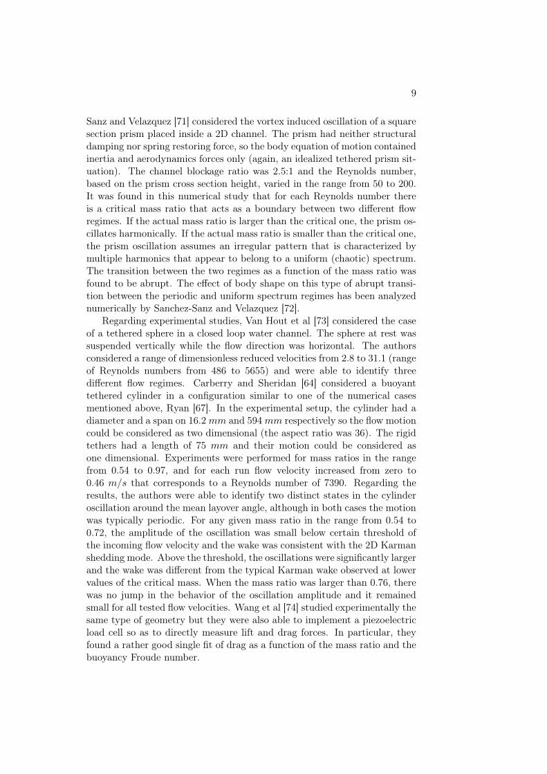
• Configuration #1 (see figure 2.2), which was considered to be the base-line. No tip clearance was allowed and the working fluid flowed parallelalong the micro-channels.

• Configurations #2, #3, and #4 (see figure 2.3). The working fluid

2.1. PROBLEM DESCRIPTION AND EXPERIMENTAL SETUP 13

Figure 2.2. Close-up view of configuration #1.

also moved parallel along the micro-channels but three different tipclearances were allowed: 250 µm, 500 µm, and 1000 µm, respectively.These tip clearances represented 50 %, 100 %, and 200 % respectivelyof the channel height (500 µm).

• Configuration #5 (see figure 2.1). The flow motion was perpendicularto the micro-channels and the tip clearance was 500 µm.

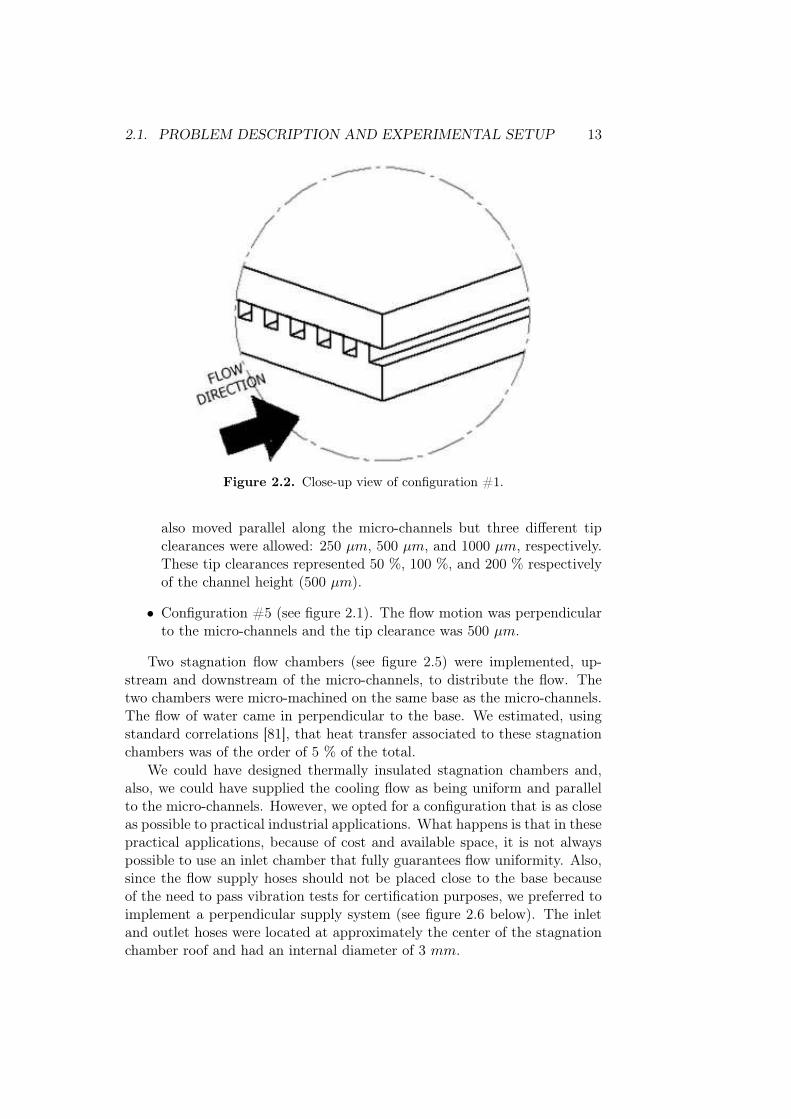
Two stagnation flow chambers (see figure 2.5) were implemented, up-stream and downstream of the micro-channels, to distribute the flow. Thetwo chambers were micro-machined on the same base as the micro-channels.The flow of water came in perpendicular to the base. We estimated, usingstandard correlations [81], that heat transfer associated to these stagnationchambers was of the order of 5 % of the total.

We could have designed thermally insulated stagnation chambers and,also, we could have supplied the cooling flow as being uniform and parallelto the micro-channels. However, we opted for a configuration that is as closeas possible to practical industrial applications. What happens is that in thesepractical applications, because of cost and available space, it is not alwayspossible to use an inlet chamber that fully guarantees flow uniformity. Also,since the flow supply hoses should not be placed close to the base becauseof the need to pass vibration tests for certification purposes, we preferred toimplement a perpendicular supply system (see figure 2.6 below). The inletand outlet hoses were located at approximately the center of the stagnationchamber roof and had an internal diameter of 3 mm.


Figure 2.3. Close-up view of configurations #2, #3 and #4.

Figure 2.4. Close-up view of configuration #5.


Figure 2.5. Schematic (top) and actual (bottom) views of the micro-channels andstagnation chambers in configurations #1-4.

Figure 2.6. Lateral view sketch of the experimental setup.


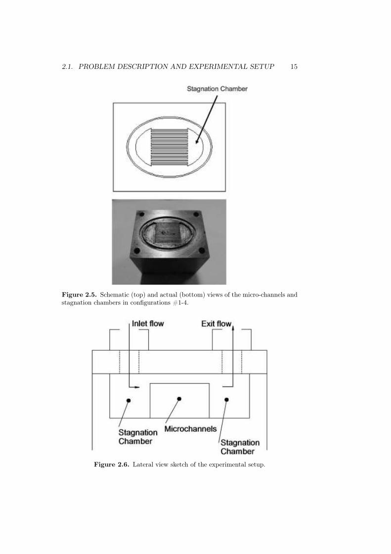
The heating system consisted of a block of aluminum alloy with an in-sertion of two electrical resistances. A PID control system was in place tomaintain the aluminum wall temperature right below the micro-channels, at70 C. Inlet water temperature was regulated to enter the micro-heat sink at35 C. An overview of the whole block is presented in figure 2.7.

In a preliminary set of experiments, the micro-heat sink and the heat-ing system were separate components joined by pressing them together witha constant mechanical force, using thermal grease at the contact surface.However, we encountered difficulties in guaranteeing the repeatability of theexperimental series. In particular, the grease film had a tendency to dete-riorate over time, probably owing to heat and surface contact pressure. Wecould have used thermal pads to solve the difficulty, but instead, we decidedto manufacture a new set of prototypes on which the heat exchange area wasmicro-machined directly on top of the heating block, which solved the issueof test’s repeatability. Ensuring a good contact between elements is, never-theless, a critical design aspect that must be dealt with in practical industrialapplications. As our experience has shown, integrated systems are superiorto those that need additional means to achieve a robust thermal contact.This good contact avoids temperature drops across the interface but due tosurface roughness effects contact spots are interspersed with gaps that are, inmost instances, air filled. That results in a global conduction coefficient thatmay be viewed as two parallel resistances: that due to the contact spots andthat due to the gaps. Increasing the joining pressure, decreasing the rough-ness of the interfaces or adding an interfacial fluid are the commonly usedmethods to decrease the gap negative effect on heat transfer. This thermalresistance is defined by [81] as Rt = (TA − TB)/q

′′

x. Although theories havebeen developed for predicting this value, the most reliable results are thosethat have been obtained experimentally.

Two T-type TC-SA thermocouples were inserted right below the micro-channels at a distance of 1.5 mm under the surface. Two additional ther-mocouples were used to measure inlet and outlet flow temperature. We re-quested to the thermocouples supplier that they all belong to the same man-ufacturing series so that the measurements errors (±0.5 C) were all basedin the same direction. Pressure drop was measured by using two pressuresensors (Ellison GS4101) that were located in the inlet and outlet hoses rightoutside the stagnation chambers. A flow-meter (GEMS FT110) was placedon the outlet hose. The total mass flux was maintained at a fixed value ineach run by the pump itself. The current in the electrical resistance was con-trolled in such a way that the temperature of the metal base was maintainedat the prescribed value. Heat losses from the base were calculated as theheat evacuated by the coolant liquid, which in turn resulted from the totalmass flux and the inlet and outlet temperatures, taking into account heatlosses in the stagnation chambers (estimated as indicated above). The dataacquisition system was a Keithley KUSB 3108. It features a variety of ana-


Figure 2.7. Overview of the heated block with micro-machined channels, poly-carbonate top wall, different insertions and supply and exit hoses.

log input/output channels, including a Cold Junction Compensation (CJC)channel, as well as digital input/output channels. The CJC channel provides1E−2 V/C with an accuracy of 1 C. The whole setup was controlled by us-ing a Proportional-Integral-Derivative (PID) algorithm as a control system,whereby inlet fluid temperature and wall temperature were held at 35 and70 C respectively. All of this programmed in LabVIEW software (short forLaboratory Virtual Instrumentation Engineering Workbench) which is a sys-tem design platform and development environment for a visual programminglanguage from National Instruments.

The PID controller compares the set-point (SP ) to the process variable(PV ) to obtain the error (e = SP − PV ), then calculates the controlleraction:

CA(t) = Kc(e+1

τi

∫ t

0edt+ τd

de

dt), (2.1)

where Kc is the controller gain, τi is the integral time and τd the derivativetime. Proportional action is the controller gain times the error. Integralaction is calculated via trapezoidal integration and is used to avoid sharpchanges when there is a sudden change in PV or SP . It is proportionalto both the magnitude of the error and the duration of the error; this term


Figure 2.8. Schematics of the experimental setup.

accelerates the movement of the process towards set-point and eliminates theresidual steady-state error that occurs with a pure proportional controller.However, since the integral term responds to accumulated errors from thepast, it can cause the present value to overshoot the set-point value. Thederivative term calculates the slope of the error over time and helps in theresponsiveness of the controlled system, but on the other hand differentiationof a signal amplifies noise and thus this term in the controller is sensitiveto noise in the error signal. The exit of PID controllers were attached to arelay to activate or deactivate the cooler fan power supply in the case of inletwater temperature controller, and the electrical resistances power supply inthe case of wall temperature controller.

A schematics of the experimental test bench is presented in figure 2.8.

2.2 Experimental results

The average results for the baseline configuration #1 (no tip clearance) aregiven in table 2.1. Six different volume flow rates G (liters per minute) wereconsidered in the range from 0.16 to 1.00 l/min. Each of these volume flowrates had an associated Reynolds number, Re, based on the average inletvelocity and hydraulic diameter of the micro-channels. Q is the evacuatedheat per unit time, QS is the ratio of Q to the platform area of the micro-heat sink (15x15 mm2 ), ∆P is the pressure drop, and PP is the pumpingpower (volume flow rate times ∆P ).

Thus, we have basically four laminar (Re 416 to 1300) and two transi-tional (Re 1959 and 2600) flows. Critical Reynolds number is found exper-

2.2. EXPERIMENTAL RESULTS 19

Table 2.1. Results of the baseline configuration #1 with no tip clearance.

Configuration 1G(l/min) Re Q(W ) Qs(W/cm2) ∆P (Pa) PP (W )

0.16 416 117 52 4907 0.0130.25 650 146 65 7251 0.0300.33 858 171 76 10456 0.0580.50 1300 221 98 16589 0.1380.75 1959 259 115 29916 0.3731.00 2600 272 121 55296 0.921

Table 2.2. Comparison between the results obtained for configurations #2 to #5and those of configuration #1.

Conf. 2 Conf. 3 Conf. 4 Conf. 5G(l/min) Q′ ∆P ′ = P ′

P Q′ ∆P ′ Q′ ∆P ′ Q′ ∆P ′

0.16 0.76 0.29 0.83 0.18 0.64 0.10 0.74 0.170.25 0.77 0.32 0.81 0.24 0.65 0.15 0.71 0.250.33 0.81 0.31 0.83 0.30 0.69 0.23 0.70 0.330.50 0.80 0.39 0.82 0.36 0.65 0.31 0.71 0.400.75 0.81 0.53 0.84 0.42 0.71 0.40 0.76 0.451.00 0.85 0.50 0.88 0.40 0.75 0.40 0.78 0.45

imentally to be approximately 2200 (see [77] thereafter transition to turbu-lence starts to take place. When characteristic length of micro-channels issmaller than 1 mm, this classical theory is not valid evidenced by experi-ments. The transition to turbulent flow occurred at Re about 1500 to 2000or even lower for smaller micro-channels [78].

The evacuated heat is in the range from 52 to 121 W/cm2, which is repre-sentative of the foreseen evolution of industrial power electronics dissipationfor the next decade or so. The chosen platform area fits the surface of theaverage heat dissipating electronic component in avionics applications. Ex-amples of current high-end line of microprocessor are an Intel Core i7-960at 3.2 GHz with a power consumption of 130 W or an AMD Phenom II X4925 at 2.8 GHz with 95 W of thermal power dissipation, so actual micro-processors are inside the range of thermal power dissipation evaluated in theexperiment.

Configurations #2-5 are considered in table 2.2, where the average resultsare provided as referred to the results of configuration #1 (the baseline). Inother words, Q′ , ∆P ′, and P ′

P are the ratios of evacuated heat, pressuredrop, and pumping power in these configurations to their counterparts inthe baseline.

The following remarks about the results presented in table 2.2 are inorder:


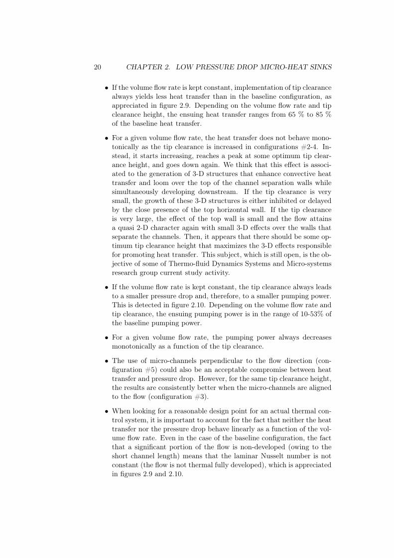
• If the volume flow rate is kept constant, implementation of tip clearancealways yields less heat transfer than in the baseline configuration, asappreciated in figure 2.9. Depending on the volume flow rate and tipclearance height, the ensuing heat transfer ranges from 65 % to 85 %of the baseline heat transfer.

• For a given volume flow rate, the heat transfer does not behave mono-tonically as the tip clearance is increased in configurations #2-4. In-stead, it starts increasing, reaches a peak at some optimum tip clear-ance height, and goes down again. We think that this effect is associ-ated to the generation of 3-D structures that enhance convective heattransfer and loom over the top of the channel separation walls whilesimultaneously developing downstream. If the tip clearance is verysmall, the growth of these 3-D structures is either inhibited or delayedby the close presence of the top horizontal wall. If the tip clearanceis very large, the effect of the top wall is small and the flow attainsa quasi 2-D character again with small 3-D effects over the walls thatseparate the channels. Then, it appears that there should be some op-timum tip clearance height that maximizes the 3-D effects responsiblefor promoting heat transfer. This subject, which is still open, is the ob-jective of some of Thermo-fluid Dynamics Systems and Micro-systemsresearch group current study activity.

• If the volume flow rate is kept constant, the tip clearance always leadsto a smaller pressure drop and, therefore, to a smaller pumping power.This is detected in figure 2.10. Depending on the volume flow rate andtip clearance, the ensuing pumping power is in the range of 10-53% ofthe baseline pumping power.

• For a given volume flow rate, the pumping power always decreasesmonotonically as a function of the tip clearance.

• The use of micro-channels perpendicular to the flow direction (con-figuration #5) could also be an acceptable compromise between heattransfer and pressure drop. However, for the same tip clearance height,the results are consistently better when the micro-channels are alignedto the flow (configuration #3).

• When looking for a reasonable design point for an actual thermal con-trol system, it is important to account for the fact that neither the heattransfer nor the pressure drop behave linearly as a function of the vol-ume flow rate. Even in the case of the baseline configuration, the factthat a significant portion of the flow is non-developed (owing to theshort channel length) means that the laminar Nusselt number is notconstant (the flow is not thermal fully developed), which is appreciatedin figures 2.9 and 2.10.


• When considering the combined behavior of heat transfer and pressuredrop, the most favorable results are obtained with the lower volumeflow rates. For example, configuration #3 (tip clearance height equalto 500 µm for a channel height of 500 µm) with the lowest volume flowrate of 0.16 l/min (equivalent to Re = 416 in the baseline configura-tion) yields a heat transfer that is 83 % of the baseline configurationwhile the pumping power has been reduced to only 18 % of the base-line (it has been divided by a factor of 5.5). In this situation, the heattransfer is 43 W/cm2, which still represents a large improvement overconventional plates of fins used for thermal control purposes of avion-ics equipment. In these conventional systems, the typical heat transferrate at the component level is in the range from 2 to 5 W/cm2. Whenconsidering the same configuration at a higher volume flow rate (0.50l/min, equivalent to Re = 1300 in the baseline configuration), the heattransfer is 83 % of the baseline configuration while the pumping powerhas been divided by a factor of 3.3. In this case, the actual heat trans-fer is 81 W/cm2. The benefit of the tip clearance is not so clear at thelargest flow rate, as distinguished in figure 2.11, where the heat trans-fer rate is plotted vs. the required pumping power. This is due to theflow topology, which is quasi-two dimensional at the upper part of thechannel. A better performance of configurations with a tip clearanceat large flow rates would require enhancing three-dimensional convec-tion at the upper region of the channel, which is the object of currentresearch.

• In any event, configuration #3 outperforms the baseline configurationfor thermal efficiencies smaller than 90 W/cm2. Figure 2.11 illustrateswell the main advantage of the tip clearance, and the fact that config-uration #3 seems to be the best choice. For instance, for a thermalefficiency of 65 W/cm2, the pumping powers associated with config-urations #1 and #3 are 3.1 and 2.0 W , respectively, which meansthat configuration #3 requires about 33% less pumping power thanconfigurations #1for the same heat evacuation target.

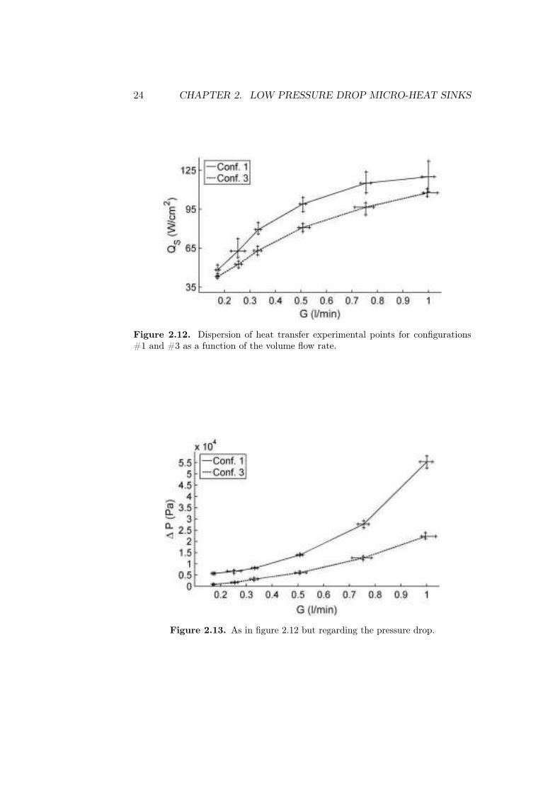
Regarding the repeatability of the results, we performed three experimen-tal campaigns for each configuration and each flow rate. In each campaignwe acquired thirty measurements timely equidistant. The dispersion of ex-perimental heat transfer and pressure drop results for configurations #1 and#3 are presented in figures 2.12 and 2.13 below, where it is seen that thedispersion in the measured volume flow rate was of the order of ±5%. Theactual dispersion of heat transfer results around configuration #1 was of theorder of ±6%, while it was significantly smaller (±2.6%) for configuration#3 and the other configurations, not represented in figure 2.12. A closer lookat the time series shows that the larger dispersion in the baseline configura-tion is associated with unsteady effects, which are enhanced to a larger level


Figure 2.9. Heat transfer in configurations #1-5 vs the volume flow rate.

Figure 2.10. Heat transfer in configurations #1-5 vs the volume flow rate.


Figure 2.11. Heat transfer in configurations #1-5 vs the pumping power.

in configuration #1 because the effective Reynolds number is larger. TheFourier transformation of all time series peaks at a frequency that is slightlylarger than that of the data acquisition system, which is 2.5 Hz. This ismuch smaller than the frequencies associated with relevant unsteady effects,namely the frequency of the volumetric pump, which ranges between 60 and70 Hz, depending on the volume flow rate, and the inverse of the convec-tive hydrodynamic time, t−1

c = Reµ/(ρCL) which ranges from 50 to 350 Hzdepending on the Reynolds number. The observed dispersion is seeminglydue to hydrodynamic instabilities. This generates local eddies that increaseviscous dissipation (and thus, also increase pressure drop) but mainly pro-mote local mixing, instead of the overall transverse convection that wouldbe necessary to increase heat transfer from the hot walls to the bulk.

At this stage, it is worth mentioning the conclusions drawn by Min et al.[16] in their numerical study of a somewhat similar problem. In particular,they found that for a fixed pumping power, thermal resistance is minimized(the optimum design point) when the ratio of tip clearance to channel widthis 0.6 approximately. Our problem was different in the sense that we did notfix pumping power but measured it (it was not a constraint in our setup)and, also, because the experimental nature of our work did not allow for anearly continuous variation of the tip clearance, as can be done in a numericalstudy. Nevertheless, we found that our optimum tip clearance (see table 2.2)would be somewhere inside the span of 0.5-1.0 of the ratio of tip clearanceto channel width, thereby coinciding qualitatively with the results of Min etal. [16]. The case of pin tip clearance seems to be different for a numberof reasons that have to do, mostly, with geometrical considerations. In thiscase, Rozati et al. [20] have reported that the optimum tip clearance in thelow Reynolds number regime would be 0.3 times the pin diameter (somewhat


Figure 2.12. Dispersion of heat transfer experimental points for configurations#1 and #3 as a function of the volume flow rate.

Figure 2.13. As in figure 2.12 but regarding the pressure drop.

2.3. CONCLUSIONS 25

similar to the fin width).

2.3 Conclusions

We have studied the effect of tip clearance on micro-channel flow based ther-mal control systems when, owing to engineering design restrictions, the flowitself cannot be considered as fully developed. The study has accountedfor two parameters of practical interest, namely the heat transfer and thepressure drop (which is related to the pumping power). Four configurationsinvolving a tip clearance have been analyzed and compared to a baselineconfiguration of micro-channel flow without tip clearance. The baseline con-figuration consists of a 15 parallel micro-channels of 15 mm of length andseparated by a step of 1 mm. The height of the square section micro-channelswas 500 µm. Tip clearances of 250 µm, 500 µm, and 1000 µm were consid-ered. One additional configuration with the channels perpendicular to themain flow and a tip clearance of 500 µm was also studied. For each configu-ration, six different volume flow rates were considered. These flow rates, inthe case of the baseline configuration, led to Reynolds numbers in the rangefrom 416 to 2600, containing both laminar and transient regime flows.

The main conclusion of the work that has been presented is that theimplementation of tip clearance in active micro-channel based thermal con-trol systems is an attractive option from the practical industrial applicationstandpoint owing to two arguments:

• The added manufacturing cost is negligible since most of the manufac-turing complexity is associated to the micro-machining of the micro-channels, while the top wall can be easily set at a lower or higher heightwith no extra cost of maintenance.

• The deterioration in heat transfer caused by the tip clearance is smallwhile the savings in pumping power are large. In our study, for theoptimum tip clearance height, the heat transfer (at the lowest volumeflow rate, Re = 416) was 83 % of the baseline configuration. However,the required pumping power was only 18 % of the baseline case. Theadvantage of introducing a tip clearance can also be illustrated notingthat the required pumping power can almost be halved maintainingthe thermal efficiency. At a larger volume flow rate (Re = 1300), theheat transfer behaved similarly while the pumping power was 36% ofthe baseline configuration.

Regarding future work, there are three related issues to be analyzed: a)the existence of an optimum tip clearance height that, seemingly, has to dowith stability issues within the fluid; b) the feasibility of enhancing three-dimensional convection in the tip clearance flow region, which could be done


manufacturing some obstacles in the top wall aiming to generate 3-D flowdisturbances that promote heat transfer with a limited pressure drop; c) tofurther understand the unsteady nature of the dispersion of results, which ishigher in the baseline configuration than in those with tip clearance.

2.4 Tables of experimental data

In this appendix whole data obtained in the experiments is presented. Rey-nolds number (Re), Nusselt number (Nu) and convection heat transfer co-efficient (h) are also shown and has been calculated via these equations:

Re =ρfCvmed

µf

, (2.2)

h =Q

Awet∆Tm, (2.3)

∆Tm =(Twall − Tout)− (Twall − Tin)

ln Twall−Tout

Twall−Tin

, (2.4)

Nu =hC

κf. (2.5)

In formulas 2.2 to2.8 , vmed is the mean velocity of the fluid, Twall,Tin and Tout are the wall temperature, inlet flow temperature and outletflow temperature respectively, all of them measured by thermocouples asindicated in the experimental setup. ρf , µf and κf are the density, viscosityand the thermal conductivity of water respectively. Water density has beenconsidered constant with a value of 995 kg/m3 and viscosity and thermalconductivity have been treated as temperature dependent variables via thesequadratic equations [81]:

µ = µ(Tin)(1 + µ1T + µ2T2), (2.6)

κ = κ(Tin)(1 + κ1T + κ2T2), (2.7)

where (in the temperature range considered), the coefficients are thefollowings:

µ1 = 1.1292, µ2 = −0.49036, κ1 = −0.1572, κ2 = 0.04704. (2.8)

2.4. TABLES OF EXPERIMENTAL DATA 27

Table 2.3. Summary of data obtained from experiments.

G (l/m) Re Tout (K) Q (W ) PP (W ) h (W/(m2K)) Nu

Configuration #10.16 415.9 318.5 117.0 4907.0 11775.1 9.20.25 649.8 316.4 146.0 7251.0 14128.9 11.00.33 857.7 315.4 171.0 10456 16274.2 12.70.50 1299.5 314.3 221.0 16589.0 20642.2 16.10.75 1949.3 313.0 259.0 29916.0 23642.7 18.51.00 2599.1 311.9 272.0 55296.0 24415.1 19.1

Configuration #20.16 415.9 316.0 88.9 1423.0 6407.3 5.00.25 649.8 314.5 112.4 2320.3 7890.0 6.20.33 857.7 314.0 138.5 3241.4 9651.1 7.50.50 1299.5 313.1 176.8 6469.7 12127.7 9.50.75 1949.3 312.0 209.7 15855.5 14148.0 11.11.00 2599.1 311.3 231.2 27648.0 15422.7 12.0

Configuration #30.16 415.9 316.7 97.1 883.3 7090.2 5.50.25 649.8 314.8 118.2 1740.2 8347.4 6.50.33 857.7 314.2 141.9 3136.8 9914.0 7.70.50 1299.5 313.2 181.2 5972.0 12456.6 9.70.75 1949.3 312.2 217.5 12564.7 14706.6 11.51.00 2599.1 311.4 239.3 22118.4 15996.1 12.5

Configuration #40.16 415.9 314.7 74.9 490.7 5278.9 4.10.25 649.8 313.4 94.9 1087.7 6549.6 5.10.33 857.7 313.1 118.0 2404.9 8101.1 6.30.50 1299.5 312.1 143.6 5142.6 9704.3 7.60.75 1949.3 311.5 183.9 11966.4 12305.2 9.61.00 2599.1 310.9 204.0 22118.4 13526.5 10.6

Configuration #50.16 415.9 315.8 86.6 834.2 6215.7 4.90.25 649.8 314.0 103.7 1812.75 7214.0 5.60.33 857.7 313.2 119.7 3450.5 8228.5 6.40.50 1299.5 312.5 156.9 6635.6 10664.6 8.30.75 1949.3 311.8 196.8 13462.2 13222.9 10.31.00 2599.1 311.0 212.2 24883.2 14092.9 11.0

Table 2.4. Constant parameters in the experiments.

Tin (K) Twall (K) C (m) L (m)308 343 0.0005 0.015


Chapter 3

MICRO-EVAPORATOR

BASED HEAT SPREADERS

The work presented in the present chapter deals with an experimental andtheoretical/numerical study of a vapour chamber heat spreader intended foravionics applications. Three configurations were considered and comparedamong themselves. First, a finned metallic flat plate was considered as thereference configuration. This was because it represented the conventionalindustrial approach. Then, a vapour chamber heat spreader was studiedhaving the same global dimensions as the reference configuration. The issueof trying to keep the same global volume is important because, in practice,the heat spreaders/heat sinks are inserted in between two Printed CircuitBoards (PCB) inside avionics boxes. Also, a second vapour chamber heatspreader with larger volume (that needed a larger separation distance be-tween electronics boards) was studied for comparison purposes. Pertainingto the field of avionics applications, all configurations were tested and stud-ied in a vertical position. However, in some cases, the off-design behavior ofthe system was studied in a horizontal position to simulate the situation ofhigh operational angles of attack that may appear, for example, in helicopterflight. Boiling inside the vapour chamber was enhanced by implementing amini-evaporator area made up of an array of mini-fin-pins having the dimen-sions of 1 cubic millimeter.

Additionally, the experimental results were also used to calibrate a theo-retical and numerical model that was developed to assist in the engineeringdesign of this type of heat spreaders. To illustrate the method capability, anoptimization process was carried out to search for the minimum weight heatspreader (that is an important design criterion for avionics equipment) thatis compatible with a series of design requirements.

The chapter organization is as follows: the following chapter deals withthe description of the problem and the experimental setup; then, the experi-mental test bench and results are presented. Next, the theoretical/numerical

29

30 CHAPTER 3. MICRO-EVAPORATOR BASED HEAT SPREADERS

model is described step by step and, finally, conclusions are stated.

3.1 Problem description and experimental setup

The problem under consideration was the comparative study of one referencemetallic heat sink, labeled HS0, and two vapour chamber based heat spread-ers, labeled HS1 and HS2 respectively, under a variety of conditions typicalof avionics applications. The description of the three different configurationsis as follows:

The reference configuration HS0 was a finned plate (60 fins) manufac-tured on aluminum alloy (thermal conductivity equal to 170 W/mK) thatweighed 480 g. A plate-fin heat exchanger has been chosen due to the factthat it is widely used in many industries, including the aerospace industry forits compact size and lightweight properties; emphasizing its relatively highheat transfer surface area to volume ratio. The dimensions of the rectangularfins were 140 mm x 12 mm x 1 mm. An overall impression of the referenceconfiguration HS0 is presented in figure 3.1 a and b. The total volume occu-pied by the reference configuration was 405,720 mm3. The spacing betweenfins was chosen after a standard design used in the aeronautics industry. Thepitch (2.2 mm) is small but it was decided to keep it as it is, and not tooptimize it, so as to have a reference case as close as possible to an actualindustrial application case. As it can be observed in figure 3.1b, a squareprism of 10 mm x 10 mm area was placed on the back of the heat sink.This prism was hollow and an electrical resistance was inserted into it. Inthis way, by means of controlling the voltage passing through the resistance,a hot spot that simulated a high thermal dissipation electronics componentwas generated at the back of the heat sink. Following the standard practicein avionics applications, to allow for sufficient additional space for electricconnections, a high conductivity aluminum plate (35 mm x 35 mm, see fig-ure 3.1b) was located between the hot spot and the back of the heat sink,attempting to smooth the temperature distribution that the fin plate receivefrom the microprocessor. This part works as a heat spreader based on con-duction and so it is most often simply a plate made of copper, which hasa high thermal conductivity (around 400 W/mK) or another material withgood thermal properties such as aluminum.

The first heat spreader configuration, HS1, also manufactured in alu-minum alloy, weighed 650 g and occupied the same volume as HS0, wasmade up of two halves, see figure 3.2 a and b:

The global dimensions of this configuration HS1 were the same as thoseof HS0. The number and the spacing of fins were also the same. Accord-ingly, to keep the same total volume, fin height was 7 mm instead of 12 mm.Hot and cold plate thicknesses, ehp and ecp were 3 mm and 2 mm respec-tively (see figure 3.2b); hot plate is referred to the aluminum plate that is


Figure 3.1. a) Front view of configuration HS0 (distances are measured in mm).b) Back view of the reference configuration.

Figure 3.2. a) Front view of configuration HS1. b) Top view of configurationHS1.


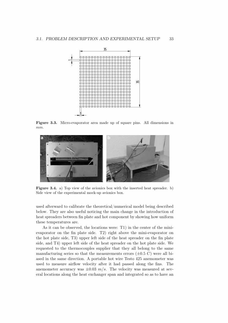
in contact with the microprocessor (actually with the heat spreader used bythe microprocessor) and thanks to the aluminum thermal conductivity, theglobal temperature is high; the cold plate is the opposite aluminum plate,both hold a volume that will work as a vapour chamber. Figure 3.2a andb show that the assembling of the two halves of configuration HS1 left aclosed empty space between the plates that forms the vapour chamber. Thedimensions of this empty space (the vapour chamber) were 180 mm x 130mm x 3 mm. In the lower part of the vapour chamber, and located op-posite the prism carrying the electrical resistance inside (the hot spot), amini-evaporator area was manufactured (see figure 3.3). This region had asize of 35 mm x 35 mm (it matched the high conductivity aluminum platelocated at the opposite side of the heat spreader wall) and it contained 324mini-fin-pins. The dimensions of the prismatic pins were 1 mm x 1 mm x 1mm, and the spacing between them was, also, 1 mm.

The working liquid used in the vapour chamber was HFE-7100 suppliedby 3M Novec. Its boiling point temperature at 1 bar was 61 C. The vapourchamber was filled with liquid up to two thirds of its height (90 mm formthe bottom of the chamber). The operations manual of the 3M Novec En-gineered Fluid HFE-7100 provided by the manufacturer explicitly states itscompatibility with aluminum. Air was extracted mechanically to ensure thatthe gas present in the vapour chamber was HFE-7100 vapour only. Some ofthe most important properties (liquid density, thermal conductivity, liquidspecific heat and vapour pressure) of the fluid are given by the manufacturerand they are shown mathematically below:

ρfHFE−7100 = 1538.3− 2.269(T − 273.15),

κHFE−7100 = 0.073714− 0.00019548(T − 273.15),

cpfHFE−7100 = 1133 + 2(T − 273.15),

ln pvapourHFE−7100 = 22.415− 3641.9

T. (3.1)

The second heat spreader configuration HS2 was like HS1 except for thefact that fin height was 12 mm. Accordingly, this configuration, that weighed780 g, filled a volume that was 1.5 times the volume of configurations HS0

and HS1. The wet area of this configuration is equal to the wet area of thefinned plate but with the heat distribution of the first heat spreader (HS1).

As explained above, all configurations were inserted and tested betweentwo boards inside a mock-up avionics box. A top view and a general view ofthe experimental set up are shown in figure 3.4a and b. In the installation ofthe HS2, the two boards have to be separated the pertinent distance leavinga gap between heat exchanger sides and boards of 1.5 mm.

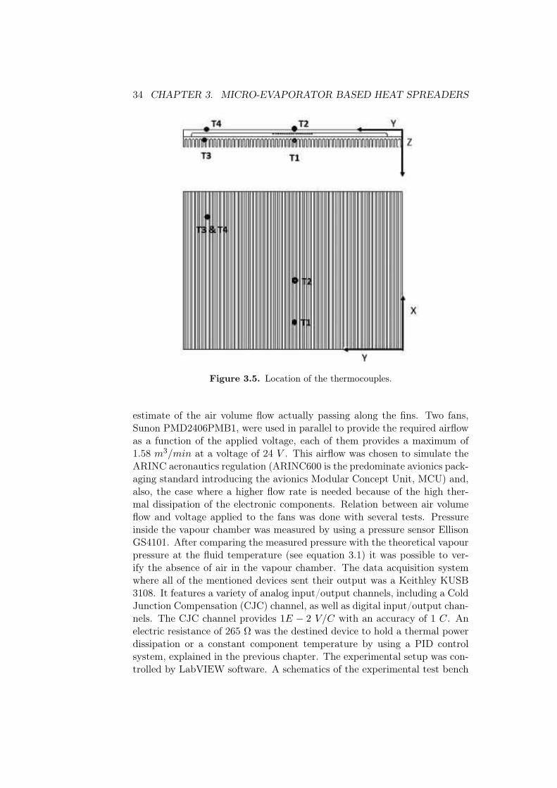
Four T-type TC-SA thermocouples (labeled T1 to T4) were inserted atthe locations shown in figure 3.5. These temperature measurements were


Figure 3.3. Micro-evaporator area made up of square pins. All dimensions inmm.

Figure 3.4. a) Top view of the avionics box with the inserted heat spreader. b)Side view of the experimental mock-up avionics box.

used afterward to calibrate the theoretical/numerical model being describedbelow. They are also useful noticing the main change in the introduction ofheat spreaders between fin plate and hot component by showing how uniformthese temperatures are.

As it can be observed, the locations were: T1) in the center of the mini-evaporator on the fin plate side. T2) right above the mini-evaporator onthe hot plate side, T3) upper left side of the heat spreader on the fin plateside, and T4) upper left side of the heat spreader on the hot plate side. Werequested to the thermocouples supplier that they all belong to the samemanufacturing series so that the measurements errors (±0.5 C) were all bi-ased in the same direction. A portable hot wire Testo 425 anemometer wasused to measure airflow velocity after it had passed along the fins. Theanemometer accuracy was ±0.03 m/s. The velocity was measured at sev-eral locations along the heat exchanger span and integrated so as to have an


Figure 3.5. Location of the thermocouples.

estimate of the air volume flow actually passing along the fins. Two fans,Sunon PMD2406PMB1, were used in parallel to provide the required airflowas a function of the applied voltage, each of them provides a maximum of1.58 m3/min at a voltage of 24 V . This airflow was chosen to simulate theARINC aeronautics regulation (ARINC600 is the predominate avionics pack-aging standard introducing the avionics Modular Concept Unit, MCU) and,also, the case where a higher flow rate is needed because of the high ther-mal dissipation of the electronic components. Relation between air volumeflow and voltage applied to the fans was done with several tests. Pressureinside the vapour chamber was measured by using a pressure sensor EllisonGS4101. After comparing the measured pressure with the theoretical vapourpressure at the fluid temperature (see equation 3.1) it was possible to ver-ify the absence of air in the vapour chamber. The data acquisition systemwhere all of the mentioned devices sent their output was a Keithley KUSB3108. It features a variety of analog input/output channels, including a ColdJunction Compensation (CJC) channel, as well as digital input/output chan-nels. The CJC channel provides 1E − 2 V/C with an accuracy of 1 C. Anelectric resistance of 265 Ω was the destined device to hold a thermal powerdissipation or a constant component temperature by using a PID controlsystem, explained in the previous chapter. The experimental setup was con-trolled by LabVIEW software. A schematics of the experimental test bench


Figure 3.6. Sketch of the experimental setup.

is presented in figure 3.6.

3.2 Experimental results

Cases considered were forced (the normal type of operation) and natural(to account for airflow system malfunctioning) convection conditions. Thethermal power dissipation of the system was measured as a function of thecomponent (hot spot) temperature and airflow volumetric rate.

Considering forced convection, figure 3.7a, b and c show the thermalpower dissipation associated to three component temperatures: 80, 90 and100 C, for the three experimental configurations HS0, HS1 and HS2. Thetests were repeated three times for each operating point in order to pointout repeatability. Ambient temperature was 25 C. The spread of the mea-surements has been represented in figures 3.7 a, b and c using vertical bars.

It can be observed that the vapour chamber heat spreader is always moreefficient than the metallic fin plate. Also, when comparing any two configura-tions, the absolute increase in efficiency, measured in watts, does not dependon the airflow velocity. For example, when the component temperature is80 C, configuration HS1 allows for a heat removal rate that is 6 W higherthan in the reference configuration HS0, no matter what the air velocity is.When the component temperature is 100 C, configuration HS2 removes 25W more than the reference configuration HS0 with no influence from the airvelocity. The heat removal capability of the vapour chamber heat spreaderis linked to the total fin area. Configuration HS1 occupies the same volumeas the reference configuration HS0 but its fin area is smaller (by a factorof 0.5) because of the allowance for the vapour chamber volume. Then, inthis case, HS1 improves HS0 by 6 W only, no matter what the component


Figure 3.7. a) Dissipated thermal power as a function of the heat spreader con-figuration and air flow volume rate, G, for a component temperature of 80 C. b)As in figure 3.7a, but with component temperature equal to 90 C. c) As in figure3.7a, but with component temperature equal to 100 C.


temperature is. However, the fin area of configuration HS2 is the same asthat of the reference configuration HS0 and, in this case, the improvementcan be as high as 25 W for the higher component temperature. Regardingthe dispersion of the results, the average spread was ±2 W that, dependingon the actual value of the heat transfer rate, represents a deviation that isof the order of ±2 % to ±3 % of the average values.

In regard to natural convection, figure 3.8 shows the thermal power dis-sipation results obtained in the natural convection case as a function of thecomponent temperature for the three configurations. It could be observedthat, in this case, the heat spreader performance is also superior to the finplate. Furthermore, the relative gains are larger than in the case with forcedconvection. In fact, the heat transfer rate gain (similar for both configura-tions HS1 and HS2) varies between 35% and 25% depending on the compo-nent temperature when compared to the reference configuration HS0. Thisfact suggests that a convenient application of vapour chamber based heatspreaders is for natural convection related thermal control. Specifically, thisis important for avionics applications because, even though the normal modeof operation is in forced convection conditions, safety regulations require thatthe system has to survive a certain time span relying on natural convectiononly. The reason is to account for a possible accidental failure of the airflowsupply system. Regarding figure 3.8, it is worth noting that configurationHS1, that occupies the same volume that the reference configuration HS0,is able to dissipate from 33 W to 38 W while keeping a component temper-ature in the range of 90-100 C that complies with the strict regulations ofmany on board avionics systems as the mentioned ARINC.

Additionally, the system behavior has been tested in the case when theavionics box is not placed vertically but it has fallen down either forward orbackwards, off-design operation. That is: in this situation, the heat spreaderis placed on a horizontal plane, not on a vertical plane. The results obtainedin natural convection conditions for configuration HS1 are presented in table3.1 where it could be observed that the system behavior is still quite robustin these circumstances. For example, if the component temperature is 100C, the system still dissipates 30 W after having fallen forward, α = 90 Cwith fins pointing downwards, (or backwards, α = −90 C) as compared tothe 38 W that dissipates in the nominal vertical position.

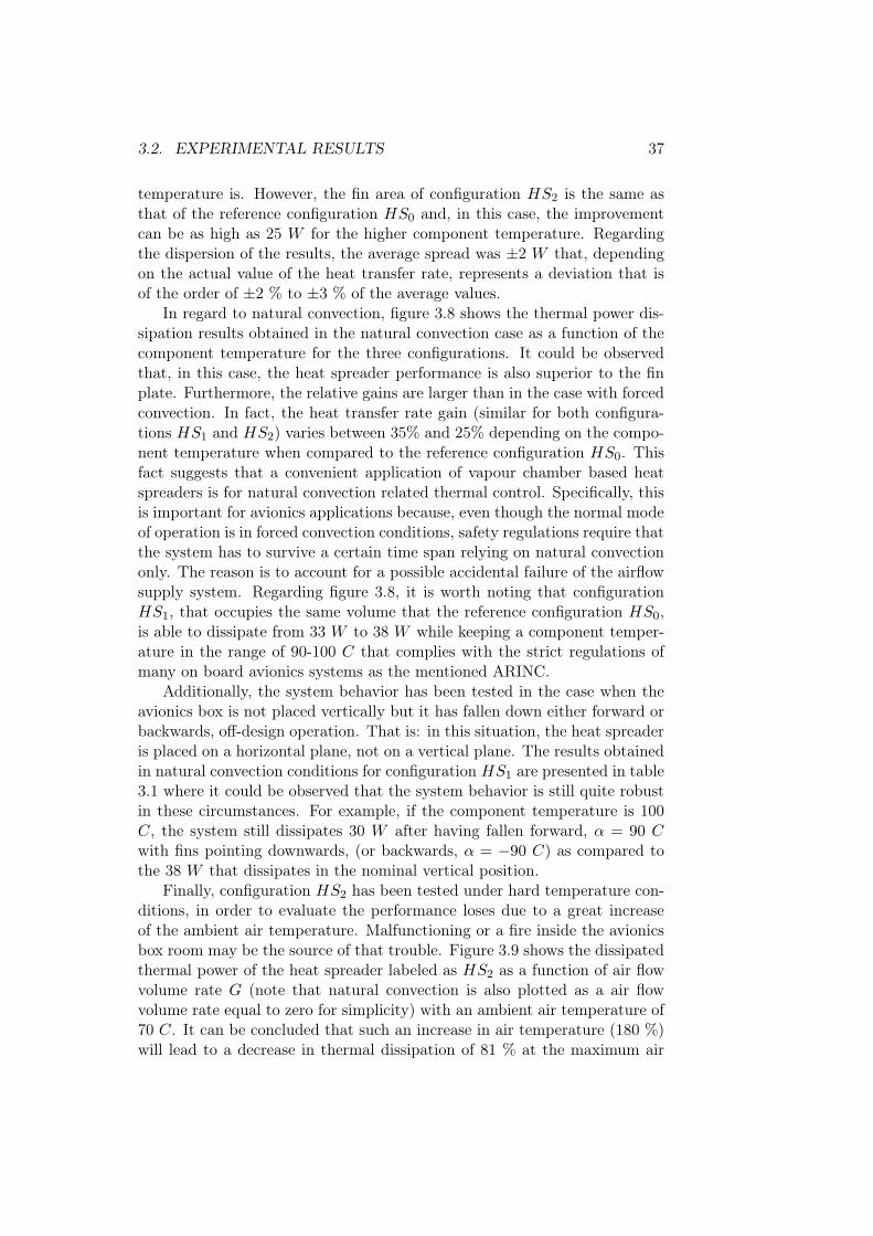
Finally, configuration HS2 has been tested under hard temperature con-ditions, in order to evaluate the performance loses due to a great increaseof the ambient air temperature. Malfunctioning or a fire inside the avionicsbox room may be the source of that trouble. Figure 3.9 shows the dissipatedthermal power of the heat spreader labeled as HS2 as a function of air flowvolume rate G (note that natural convection is also plotted as a air flowvolume rate equal to zero for simplicity) with an ambient air temperature of70 C. It can be concluded that such an increase in air temperature (180 %)will lead to a decrease in thermal dissipation of 81 % at the maximum air


Figure 3.8. Thermal power dissipation results obtained in the natural convectioncase as a function of the component temperature for the three configurations.

Table 3.1. System off-design behavior: dissipated thermal power as a function ofthe component temperature, position, and configuration.

HS0 HS1

Tcomponent(C) α(deg) Dissipated thermal power (W )

80 -90 18.7 19.380 0 22.0 26.680 90 16.3 21.790 -90 22.4 25.090 0 27.2 31.290 90 19.3 26.3100 -90 24.9 29.5100 0 32.5 36.8100 90 23.5 30.3

3.3. THEORETICAL MODEL AND SYSTEM OPTIMIZATION 39

Figure 3.9. Thermal power dissipation results for configuration HS2 with anambient temperature of 70 C.

flow rate and of 69 % in natural convection for a component temperature of90 C. With the dissipating device at 100 C, the percentages are 73 % and57 % at maximum air flow and in natural convection respectively.

3.3 Theoretical model and system optimization

A theoretical model of the vapour chamber based heat spreader has beendeveloped to be used for system optimization purposes. The aim is to per-form a trade-off between heat dissipation rate and total weight that is veryimportant for avionics applications. The theoretical model that has beendeveloped divides the system in a series of modules that simulate: 1) theheat dissipating electronic component, 2) the hot plate, 3) the vapour cham-ber, 4) the cold plate, 5) the fins, and 6) the airflow passing along the fins.Each module is formulated separately and connected to the other modulesvia the heat sources, the sink terms, and the boundary conditions. A genericoverview of the model is presented in the sketch given in figure 3.10 below:


Figure 3.10. Sketch of the heat spreader theoretical model.

The equations of the model, with the spatial coordinates defined in figure3.5, are:

3.3.1 Module 1: the heat dissipating electronic component

The thermal power P dissipated by the electronic component goes into thehot plate via thermal conduction. A thermal gel is used at the mechanicalinterface that exists between both elements. This interface has a thermalcontact resistance Rcont and its area is Acont.

P = Acont

Tcomp − Thpcont

Rcont. (3.2)

In equation 3.2, Tcomp is the temperature of the electronic componentand Thpcont

is the spatially x-y averaged hot plate temperature in the contactregion.

3.3.2 Module 2: the hot plate

The hot plate is made up of an aluminum alloy that has a high thermalconductivity (170 W/mK). Furthermore, this hot plate is flat and verythin (the ratio of the square of the surface area to the thickness is 54) so itis possible to neglect the temperature spatial derivatives in the z direction(normal to the plate). This means that the hot plate temperature Thp isfunction of x and y only.

Regarding the energy balance, the hot plate receives, on the one hand,heat from the contact region that is adjacent to the electronic component. Onthe other hand, heat leaves the hot plate via three mechanisms: a) boiling inthe finned evaporator area, b) liquid convection and c) gas convection (note


that inside the vapour chamber there is boiling and the working fluid existsin both gas and liquid phases). However, in this case, estimates of the gasconvection term prove that it is much smaller than the other two terms andhas not been included in balance equation 3.3:

ehpκp

(

∂2Thp

∂x2+

∂2Thp

∂y2

)

= (Qboiling − P )q(x, y) + ql, (3.3)

where ehp is the hot plate thickness (see figure 3.2b) and κp its thermalconductivity. Qboiling is the total heat rate transferred in the boiling pro-cess. P , as explained above, is the thermal power dissipated by the electroniccomponent. q(x, y) is a step-like function that is equal to zero outside the in-terface that connects the electronic component to the hot plate and equal to1/Acont at the interface. The dimensions of q(x, y) are m−2. The x-y integralof the function at the interface is 1. ql represents the heat convection termper unit area associated to the working fluid in liquid phase that is presentinside the vapour chamber and it is modeled using a thermal resistance thatis adjusted using the experimental results. Thus, ql = (Thp − Tcp)/Rl in theliquid wetted area and ql = 0 otherwise (Tcp is the cold plate temperaturethat is, also, a function of x and y). Equation 3.3 is integrated in a rect-angular domain of dimensions H x L (horizontal and vertical dimensions ofthe plate respectively) and its thermal boundary conditions at the four edges(x = 0 and 0 ≤ y ≤ L, x = H and 0 ≤ y ≤ L, y = 0, 0 ≤ x ≤ H, y = L,0 ≤ x ≤ H) are adiabatic.

3.3.3 Module 3: the vapour chamber

The working fluid in the vapour chamber receives heat from the hot plate(via boiling and convection) and transfers it to the cold plate (via conden-sation and convection). Since there is mass conservation and a steady-stateis assumed to hold the position of the interface liquid-vapour remains con-stant and total boiling heat transfer rate at the hot plate is equal to totalcondensation heat transfer rate at the cold plate. Therefore:

Qboiling =

∫ ∫

Ω

hcond(Tvap − Tcp)dxdy, (3.4)

where Ω refer to the wetted vapour area, Tvap = (Thpplate+ Tcpplate)/2

and hcond is the condensation heat transfer coefficient inside the vapourchamber, Tvap is the vapour temperature, and the averages are performedover the whole plate surface.


3.3.4 Module 4: the cold plate

The model approach used for the cold plate is the same as the one usedfor the hot plate (subsection 3.3.2). In particular, the cold plate receivesheat from the vapour chamber via condensation and liquid convection anddelivers it to the fins via conduction. Accordingly, its balance equation iswritten as:

ecpκp

(

∂2Tcp

∂x2+

∂2Tcp

∂y2

)

= Afκp

(

∂Tf

∂z

)

z=zf

− qin, (3.5)

where ecp is the cold plate thickness (see figure 3.2b). The term -Afκp(∂Tf/∂z) represents the thermal power that leaves the cold plate byconduction and goes into the fins. This term is evaluated at the root of thefin (z = zf). Af is the ratio of the sum of the cross fin areas to the totalplate area, and Tf is the fin temperature. qin models the heat rate per unitarea that comes from the vapour chamber into the cold plate. It is madeup of two terms: (Thp − Tcp)/Rl in the region wetted by the liquid, andhcond(Tvap − Tcp) in the region in contact with the vapour. The domain andboundary conditions for equation 3.5 are the same as for equation 3.3.

3.3.5 Module 5: the fins

The model equation for the fins represents a balance between heat conduc-tion and convection to the ambient air. The information of the cold platetemperature enters the balance equation via the boundary conditions sincefin root temperature is equal to the cold plate temperature at the same po-sition. On the other side, the fin tip and the lateral edges are assumed to beadiabatic.

efκp

(

∂2Tf

∂x2+

∂2Tf

∂z2

)

= 2ha(Tf − Ta), (3.6)

here, ef is the fin thickness, ha is the convection heat transfer coefficientwith the surrounding air, and Ta is the air temperature (25 C in this study).Equation 3.6 was integrated in rectangle of dimensions B x L where B is thefin height (see figure 3.1.a).

3.3.6 Module 6: the air

The external air behavior is modeled as it passes along the channels formedby the cold plate, the fins, and the back of the next electronics board locateinside the avionics box (see figure 3.2 and figure 3.3). The average air massflow rate m related with the air volume flow rate G and it is assumed to be


prescribed since it is controlled by the fans. Then, the air is heated up as itpasses along the fins and the balance equation 3.7 holds:

mcp,ad∂Ta

∂x= 2ha(Tf − Ta), (3.7)

where cp,a is the air specific heat and d is the distance between fins(viscous effects have been neglected). The boundary condition for equation3.7 is that Ta is equal to the ambient air temperature before entering intothe fin area Ta0 (25 C in this study).

3.3.7 Resolution

Summarizing, the model contains: a) six equations 3.2, 3.3, 3.4, 3.5, 3.6 and3.7, b) six unknowns: Tcomp, Thp(x, y), Tvap, Tcp(x, y), Tf (x, z), Ta(x, z), c)four parameters to be adjusted via the experiments: Rcont, Rl, hcond, ha, d)four series of operation parameters to be selected: d1) the dimensions of thehot/cold plates (L and H), d2) the number, spacing and size (B) of the fins,d3) the thermal power dissipated (P ) by the electronic component, and d4)the air mass flow rate m . Regarding the four parameters to be adjusted viathe experiments, the following hypothesis, Incropera and DeWitt [82], weremade regarding their behavior:

Rcont = λ1,

Nuliquid =xl

Rlka= λ2Raλ3 = λ2

(

ρ2l cp,lgβ(Tcomp − Ta0x3l )

µlkl

)λ3

,

Nucond =hcond(L− xl)

kaλ4

(

ρ2l ghfg(1 + 0.68Ja)(L− x3l )

µlkl(Tvap − Ta0)

)λ5

,

Nua =haDh

ka= λ6Reλ7 = λ6

(

mDh

µa

)λ7

,

where λ1 to λ7 are the seven coefficients to be adjusted, and Ra, Re, andJa are the Rayleigh, Reynolds and Jacob numbers. Ra and Re are basedon the hydraulic diameter Dh of the channel formed by adjacent fins and Jadefined as cp,l(Tcpplate−Tvap)/hfg. The adjustment was carried out searchingfor the set of parameters λ1 to λ7 that minimized the total deviation in aseries of experimentally measured points. The results obtained were: λ1 =39x10−5 m2K/W , λ2 = 2.0, λ3 = 0.18, λ4 = 1.2, λ5 = 0.25, λ6 = 0.27,λ7 = 0.51, and the root mean square of the deviation was 3.5%. λ1, thatrepresents the thermal contact resistance, has a value of 39x10−5 m2K/W .For comparison purposes, contact resistances of aluminum metallic interfacesare in the range of 15x10−5 m2K/W to 50x10−5 m2K/W , Incropera and


Figure 3.11. Constant weight (dashed line, Kg) and component temperature(solid line, C) contours as a function of the heat spreader dimensions (H and L).

DeWitt [82]. Nuliquid was of the order of 160 that also agrees with therange provided in reference [82]. λ4 and λ5 were 1.2 and 0.25, respectively,while the values proposed for similar cases, reference [82], are 0.943 and 0.25,respectively. Nua was in the range from 4 to 12 while empirical correlations[82], give values from 1.5 to 9. It is, nevertheless, to be noted that, in thepresent case, heat fluxes and temperature fields were not spatially constantand that the geometry differed from the idealized situation considered bymany semi-empirical correlations provided in the literature, so deviationsare to be expected.

3.3.8 System optimization

From the engineering standpoint, a theoretical/numerical model allows forthe possibility to draw performance maps and carry out an optimizationprocess. One performance map is presented in figure 3.11 where iso-contoursof the system weight and component temperature are plotted as a function ofheat spreader dimensions H and L. In this case, the prescribed parameterswere: dissipated power: 100 W , air flow rate: 15 m3/h, heat spreader width:15 mm (to fit between two adjacent electronic boards), and fin thickness,separation and height 1 mm, 2.2 mm and 5 mm respectively.

3.4. CONCLUSIONS 45

Table 3.2. Results obtained in the optimization process.

Component temp. (C) L (cm) H (cm) Number of fins Weight (g)

85 15 22.5 72 78590 15 13.2 42 58495 15 9.7 31 509100 15 8.0 26 472

As it could be observed, the iso-component temperature lines get moredensely packed when the overall heat spreader area is reduced (simultane-ously smaller H and L dimensions) suggesting, as expected, that systemperformance tends to be more sensitive to variations of the operating con-ditions when the size is decreased. It is also apparent that for a prescribedcomponent temperature, smaller weight is obtained if the heat spreader ismade taller (larger L). However, this trend has the practical limitation of thenormalized size of avionics boxes. To assist in the practical design of avionicssystems so as to find the system with minimum weight, these results can begeneralized to account for several combinations of the free design parame-ters. One example of this is shown in table 3.2 where a constant thermaldissipation of 100 W is considered.

The results presented in table 3.2 show that the optimum heat spreaderweight does not decrease linearly along with the increase in the allowed com-ponent temperature. This is better appreciated in figure 3.12 below wherethe optimum system weight has been plotted as a function of the componenttemperature. In particular, it could be observed that the rate of weight im-provement tends to decrease along with the increase in allowed componenttemperature. For example, if the component temperature is allowed to risefrom 85 to 90 C (a 5 C increase) weight can be decreased by a factor of 26%. However, if a much costlier component is used that can withstand a tem-perature of 100 C (a 15 C increase) the optimum system weight decreases bya factor of 40 % only. This fact has practical implications in the sense that,when looking simultaneously at the heat spreader thermal efficiency andweight and at the cost of the electronic components, and searching for a rea-sonable design compromise, a promising solution could be to select electroniccomponents that do not necessarily have to be very costly and sophisticate.In fact, a component that is able to withstand a temperature of 90 C mayrepresent a reasonable compromise when looking at the behavior shown infigure 3.12.

3.4 Conclusions

An experimental and theoretical/numerical study has been carried out onthe behavior of vapour chamber heat spreaders for avionics thermal control


Figure 3.12. Optimum system weight as a function of the component temperature.

purposes. In these systems, thermal efficiency has to be combined with alow system weight, a forced convection normal operating condition, and anatural convection accidental operating condition. From the thermal dissipa-tion standpoint, it was found that vapour chamber based heat spreaders aremore efficient than equivalent metallic fin plates that occupy the same vol-ume. However, from the weight point of view, metallic fin plates are lighterthan their heat spreaders counterparts. At the higher air flow rate that wasconsidered (25 m3/h), the heat spreader had a thermal efficiency 10 % betterthan the fin plate, but it was 35 % heavier. In natural convection conditions,the thermal efficiency of the heat spreader was 30 % higher than the fin plate.Higher thermal efficiencies, in forced flow conditions, of the vapour chamberheat spreader can be achieved using higher fin height. However this comesat the unwelcome expense of widening the gap existing between adjacentelectronic boards inside avionics boxes, which translates into placing fewerboards per box. For example, increasing the heat spreader volume by a fac-tor of 50 % would increase thermal efficiency by a maximum of 15 % only.Another attractive advantage of the vapour chamber heat spreader is its ro-bust off-design behavior. For example, when the avionics box topples 90 Ceither forwards or backwards, performance degradation is only of the orderof 15 %. Also, this degradation is smaller than in the fin plate case. Thedevelopment of a theoretical/numerical model of the heat spreader, coupledto an optimization algorithm showed that it is possible to save weight by afactor of the order of 20-30 % for the same heat dissipation rate. The modelalso showed that the weight reduction rate does not scale linearly with theincrease in component temperature (and cost).

Chapter 4

LOW REYNOLDS NUMBER

VORTEX STUDIES

Two particular experiments are done in this chapter. The first one deals withthe confined 3D laminar flow behavior around a fixed square section bluffbody. The second one deals with the same confined 3D laminar flow behaviorbut, this time, the square section bluff body is not fixed, the movementrestriction perpendicular to the flow has been removed. These experimentsfocus on hydrodynamic topology by using Particle Image Velocimetry (PIV)methods. These methods rely on the presence of particles in the flow thatnot only follow all flow velocity fluctuations but are also sufficient in numberto provide the desired spatial resolution of the measured flow velocity.

Both sections are organized with the same structure: first problem de-scription and experimental details are explained, then experimental mea-surements are shown and discussed and finally conclusions are provided.

4.1 Experimental study on the confined 3D laminar

flow past a square prism with a high blockage

ratio.

As a summary from the previous literature discussion shown in chapter 1,it could be said that confinement plays an important role in the flow pastan obstacle in the 2D laminar regime. Blockage ratio affects both local flowtopology, even leading to an inversion in the sequence of vortices, and globalflow parameters such as recirculation bubble size and the onset of vortexshedding. Although these results are well established, the author of thepresent dissertation believes that it is worth going a step farther so as toquantify the effect of the span-wise confinement as well. The reason is that,so far, this effect has deserved less attention in the literature even thoughit is, nevertheless, of interest from the industrial standpoint. In fact, the

47

48 CHAPTER 4. LOW REYNOLDS NUMBER VORTEX STUDIES

typical configuration in many industrial applications is the channel having anearly square cross section. As expected, confinement effects in this 3D casehave large influence on flow topology.

An experimental PIV study is presented that addresses the confined 3Dlaminar water flow behavior past a square section prism. The Reynoldsnumber, based on prism cross-section height varies between 100 and 256. Thechannel aspect ratio is 1/1 and the blockage ratio is 1/2.5. This geometryis representative of a passive method to enhance mixing in otherwise highlyordered laminar channel flow. It is found that the lateral walls exert astrong effect on the flow behavior with two main consequences: a) the onsetof vortex shedding is delayed to a Reynolds number in the vicinity of 170,as opposed to the unconfined case where the critical Reynolds number isreported to be between 50 and 60, and b) transition from the steady closedrecirculation bubble regime to the vortex shedding regime is not abrupt.In particular, there is a range of Reynolds numbers for which the closedrecirculation bubble oscillates with increasing amplitude prior to the onsetof the Karman street regime. The experimental results are supported bynumerical computations that have been performed with the aim of crosschecking results and conclusions (they have been carried out by other groupmembers). The relation of the results with the practical design of engineeringsystems is also discussed.

4.1.1 Experimental Details

Experimental set-up

The experiments were conducted in a closed-loop circuit. The working fluidwas water and the main components of the circuit were: a) a primary closedtank, b) a square section channel inserted into the tank that contained thetest section with the square prism, c) a flow meter and a valve, d) a secondaryopen tank, and e) a pump. A schematics of the circuit is shown in figure 4.1.

The flow meter was a Siemens Sitrans FM MAG1100 electromagneticflow-meter sensor with a transmitter Sitrans FM MAG5000 and it measuredin the range from 0 to 5 liters/min with an uncertainty of less than ±5 %.A magnetic flow meter is a volumetric flow meter which does not have anymoving parts and is ideal for waste-water applications or any dirty liquidwhich is conductive or water based. The operation of a magnetic flow-meteror mag meter is based upon Faraday’s Law, which states that the voltageinduced across any conductor as it moves at right angles through a magneticfield is proportional to the velocity of that conductor. As it will be shownbelow, in the characterization of the incoming flow section, the flow ratewas also measured indirectly by integrating the upstream velocity profilesobtained via PIV. The valve was used to control the volumetric flow allowingthe pump to work at their optimal power supply. The pump was an ITT

4.1. CONFINED 3D LAMINAR FLOW 49

Figure 4.1. Schematic view of the experimental set up.

Totton centrifugal pump magnetic drive DC15/5. The dimensions of boththe main tank and the test section, manufactured on methacrylate, are givenin figure 4.2. The total volume of water involved in the test was 20 ± 1 liters.A honeycomb section was inserted at the inlet of the test channel so as tohomogenize the flow as much as possible. Actual pictures of the set-up arealso presented in figure 4.2.

To quantify flow uniformity promoted by the honeycomb section, PIVmeasurements were also performed upstream of the prism. The room tem-perature of the experiments, that influences water viscosity, was 19 C. Dis-tilled water used in the experiments was left for at least three days in theroom to guarantee that it homogenized its temperature. Prior to the test, itwas checked that water temperature was 19 C as well. The volume flow ratewas varied in the range from 0.387 to 0.962 liters/min. When the Reynoldsnumber is defined based on the vortex generator cross section height andaverage inlet velocity, this volume flow yields a Reynolds number range from100 to 256.

PIV measurements

Particle Image Velocimetry (PIV) working principle is based on the mea-surement of the displacement of small tracer particles that are carried bythe fluid during a short time interval. These particles are small enough toaccurately follow the flow motion and not alter the fluid properties and big


Figure 4.2. Sketch, dimensions (in mm) and pictures of the test section and themain tank. Location of the origin of coordinates is also shown.

enough to scatter the sufficient light to get filmed by a camera. These tracerparticles are illuminated by a thin light sheet generated from a pulsed lightsource (usually a double-head pulsed laser system) and the light scatteredby them is recorded onto two subsequent image frames by a digital imagingdevice (typically a CCD camera). By means of stereoscopic imaging it ispossible to determine the three components of the flow velocity within theplanar field defined by the light sheet. The simplified one-camera systemssuffers from the restriction that the optical axis must be aligned in the direc-tion normal to the light-sheet plane, and moreover, this system only yieldstwo velocity components within the measurements plane. PIV method isthen a non-intrusive measurement method but it requires optical access forboth the delivery of the light sheet and recording of the images. A schematicview of a PIV system is shown in figure 4.3.

The PIV set used on the next experiments was a Dantec Dynamics sys-tem. Flow illumination was provided by a pulsed Nd:YAG 800 mJ laser withwavelength of 532 nm. Each laser pulse lasted for 4 ns; that time is smallenough to see particles as dots not as streaks because distance traveled bythe particle in exposure times of 4 ns is much smaller than the size of theparticle. This kind of laser, with its very short pulse duration and with pulseenergies up to almost 1 J is suitable to illuminate flows without any limit ofthe flow speed. The standard architecture of these lasers consists of two sep-


Figure 4.3. Schematic view of PIV system.

arate lasers firing independently at the required pulse separation. Howeverits repetition rate ranges between 10 and 50 Hz (15 Hz in this case) posingthe major limitation of Nd:YAG-based systems in performing time-resolvedexperiments. In the case study this is not going to be a limitation due tothe very low-speed flow (v < 0.05 m/s).

Images were taken using a Dantec Dynamics Flow Sense 2M camera witha resolution of 1600 x 1200 pixels. Data transmission was made directly tothe PC RAM via a National Instruments PCIe-1427 image acquisition boardwhich allows for an information transfer larger than 200 MB per second,which is sufficient for the information budget considered in this study. Thefrequency of images grabbing was 15 Hz so, the camera transfer 30 imagesper second which is at most 110 MB per second if the bit depth is 16bit/pixel. CPU RAM reserved for data acquisition was 4 GB, that meansa 537 pair of images per test batch. At a frequency of 15 Hz gives us a 35seconds gap of images recording. The camera lens was a Zeiss Makro-PlanarT⋆ 2/50 mm ZF. The camera was oriented perpendicular to the laser sheetand normal to the duct side wall. That means only 2 velocity components aregoing to be yielded. After passing side walls, it was verified that the thicknessof the laser sheet was smaller than 1 mm. Synchronization between imagecapturing and flow illumination was carried out using a timer box providedby Dantec Dynamics through another National Instrument Board PCI-6602timer board.

Laser pulse, image acquisition, synchronization of all components and


Figure 4.4. Example of high image density frame captured by camera with anhomogeneous seeding. Flow goes up-direction.

post-processing was carried out by Dynamic Studio software of Dantec Dy-namics.

The flow was seeded with Polyamide Seeding Particles (PSP-5) having amean diameter of 5 µm (size between 1 to 10 µm). They are non-sphericalbut round, with a density of 1.03 g/cm3. The seeding procedure consistsof increasing the concentration gradually from a low level until reaching thedesired one. If seeding exceeds the optimum level, multiple scattering andopacity compromise the setup of the experiment. It has been calculated tohave at least 10 particles per window on average (high image density) doingsome samples before each test. That means that a single particle cannot betracked (PTV) because the displacement is higher than the mean distancebetween adjacent particles. With this approach one needs to rely on statisticsto identify the most probable match of particle images in the two frames.

This type of seeding is in line with the one used in other related studiessuch as the one performed by Rehimi et al (2008). In any case, the parti-cle response time was of the order of 10−6 seconds, as computed using themethod described by Nguyen (2002) which is well below the typical thresholdcharacteristic time of the tests. Within the approximation of low Reynoldsnumber, the equation of motion of a small spherical particle immersed in afluid flow is given as:

4

3πa3ρp

dvpdt

− 4

3πa3ρf

dU

dt= −6πµa[(vp −U)− 1

6a2∇2U ]. (4.1)


This equation is known as the Basset-Boussinesq-Oseen (BBO) equationwhere only quasi-steady viscous term (Stokes drag) is evaluated. Thanksto the small size of the particle tracers used in PIV, the right hand side ofthe equation 4.1 is the term which dominates in the original BBO equationthat can be found in [76]. In this equation vp is the particle vector velocity,U is the velocity of the surrounding fluid, a is the particles mean radiusand ρp and ρf are the densities of particles and fluid respectively. In the

approximation that dUdt

=dvp

dt, the difference between the particle velocity

vp and that of the surrounding fluid U can be estimated as:

(vp −U) =2

9

a2(ρp − ρf )

µ

dvpdt

, (4.2)

where the velocity difference vp − U is referred to as the slip velocity.Clearly from 4.2 the choice of neurally buoyant particles (ρp − ρf )/ρf = 0leads to particle tracers that accurately follow the flow. In our case, (ρp −ρf )/ρf = 0.03, that means our particles are going to have a good accuracyfollowing water flow. The characteristic response time is defined as τ =29a2(ρp−ρf )

µ, and is equal to 4.1E-8 s with these particles, which is smaller than

the smallest time scale of the flow that is of the order of tenths of second andthe double pulse delay time (5 ms). The ratio between these characteristictimes is known as particle Stokes number Sk. From a practical point ofview, it can be stated that the condition Sk < 0.1 returns an acceptable flowtracing accuracy with errors below 1 %. Regarding the scattering propertiesof tracer particles, particle diameter is larger than the light wavelength (532nm) so it is the Mie regime where there is no problem with scattering oflight. In this regime most of the light is scattered in the forward directionand an appreciable amount of light backward direction, while at an angleof 90 degrees the amplitude of scattered light is generally very low. That iswhy for a single-camera PIV with the optical axis normal to the light-sheetplane use a much stronger light source than other particle-based techniques.

PIV measurements were carried out in twelve different areas: six of themlocated upstream and another six downstream of the prism. Upstream anddownstream areas were aligned among themselves. Their large size preventedthe possibility of using a single area covering the upstream, the prism, and thedownstream regions simultaneously; this is why upstream and downstreaminterrogation areas were treated separately. A front view (looking from the“y” direction) of their location is presented in figure 4.5. Interrogation areaswere placed in the following planes: z = −12.5 mm, z = −6.5 mm, z = −1mm, x = 5 mm, x = −1 mm and x = −6.5 mm respectively. Two of theseplanes (see figure 3) were aligned with the main axes of the channel section,another two were located near the walls, and the remaining two were placedin the intermediate region.


Figure 4.5. View from the “y” direction of the duct with the prism and theinterrogation areas.

A 3D view of all six upstream areas is presented in figure 4.6. However,to keep a clear representation, only two of the downstream areas are shown infigure 4.7. In what follows, all distances will be made dimensionless using theprism cross section height, 10 mm, as the characteristic length (also in thenumerical simulations to be described below). In figure 4.7, the dimensionlesscoordinates of test points are: P1 (0, 5, -1.25), P2 (0, 4, -1.25) and P3 (0,6, -1.25). The flow information associated to these three points will be usedin a forthcoming section. All areas had the same physical dimensions: 80mm x 25 mm, and each of them contained 1600 x 500 pixels. In all cases,each experiment was repeated three times to assess the repeatability of theresults.

Once the recorded images are stored, it is time to process them. Thisconsists essentially of a cross-correlation analysis of the particle-image pat-terns in small sub-domains , or interrogation regions, between the first andsecond image frame. The particle-image displacement divided by the im-age magnification and the time delay between the laser light pulses yieldsthe local fluid velocity. This process is repeated for the entire image do-main which yields the instantaneous velocity in a planar cross section of theobserved flow. Two additional post-processing methods are implicitly donewhen images are being analyzed, image restoration and image enhancement.The first one attempts to repair undesirable effects due to the imaging, thesecond one accentuates certain image features. Such post-processing includeslow-pass and high-pass filtering, histogram equalization, min/max filtering...

Sampling of the flow field was carried out at a frequency of 15 Hz. Eachsample was generated by processing the information associated to two laserpulses separated 5 milliseconds in time. Then, in the case of the highestReynolds number (256), where the mean flow velocity was 0.024 m/s, a par-


Figure 4.6. View of the six upstream PIV areas.

Figure 4.7. View of two downstream PIV areas and the location of test pointsP1, P2 and P3.


ticle would travel at the order of 0.12 mm between consecutive pulses in thestream wise direction that is a distance much smaller (by two orders of mag-nitude) than the characteristic length of the problem (the prism cross sectionheight of 10 mm). Each PIV area was divided into smaller sub-interrogationareas of 6 mm x 6 mm containing 128 pixels x 128 pixels each one thatcorrespond to 21 pixel per millimeter. The post-processing software allowedfor a parallel self-consistent re-computation of the flow field in successiveinterrogation windows of 64 pixels x 64 pixels (3 mm x 3 mm), 32 pixels x32 pixels (1.5 mm x 1.5 mm) and 16 pixels x 16 pixels (0.8 mm x 0.8 mm).That is, in the end, a velocity vector was computed for each window of 0.8mm x 0.8 mm and this computation was consistent with the computationsperformed at the larger windows. Furthermore, the software allowed for thepossibility of performing flow computations at smaller windows of 8 pixel x8 pixel (0.4 mm x 0.4 mm) and so on. However, these finer computationswere not carried out because, in this case, the typical distance traveled byflow particles at the highest Reynolds number (0.12 mm) was of the sameorder of magnitude as the window size. Then, it could be stated that thefinal flow resolution of the experimental tests was of the order of 1 mm thatis considered to be sufficient to describe the phenomena being analyzed. Anoverlap of 50 % of the sub-interrogation windows size was also implementedimproving measurement accuracy and vector map resolution.

Regarding the time resolution, it will be shown in a later section that thetypical frequency of the large scale vortical structures being observed was0.7 Hz that correspond to a characteristic time of 1.5 s. In this regard, eachrecording sequence consisted of 500 frames separated 0.067 s in time fromeach other (15 Hz) and lasting for a total of 33.5 s. Then, the characteristictime of the observed phenomena was of the order of 20 times larger than thesampling time and, also, 20 times smaller than the total recording time.

For a given particle image in the first frame, each particle image in thesecond frame is a possible match candidate and each pair represents a pos-sible displacement with equal likelihood. This procedure is repeated for allparticle image in the interrogation domain in the first frame, and the proba-bilities in the displacement peak for each of the matching pairs will soon bedominant over the displacement peaks for unrelated pairs. Two importantrequirements for PIV interrogation are evident: a) the displacement of theparticle images within the interrogation domain should be uniform; and b)the interrogation domain should contain a considerable number of particleimage pairs (that is why these tests were done with high-image density).

It is clearly concluded from figure 4.8 in the right, that the displacementof particles goes unidirectional to the positive side of one axis. The methodjust described is called adaptive correlation, figure 4.8 shows an example ofadaptive correlation on a pair of frames.


Figure 4.8. Histogram analysis for finding the most probable displacement.

4.1.2 Results and discussion of the PIV measurements

Laminar duct flow in the clean configuration without the prism

First of all, the flow in the duct has been characterized without the obstacle.The volume flow rate was measured using three different approaches: onedirect and two indirect. They were:

• Measurement 1: direct flow meter lecture.

• Measurement 2: Integration of the PIV results (A). Specifically, in-tersection of the six upstream interrogation areas shown in figure 4.6,together with the fact that the incoming flow had two planes of symme-try, yielded experimental information on the stream wise “y” velocity“v” in a grid of 25 points inside the channel section, see figure 4.10. ThePIV “v” velocity data at these points was used to generate a fifth orderleast squares fitted parabolic profile of the type shown in equation 4.3.Then, this profile was integrated along the “x” and “z” coordinates anda volume flow rate was computed.

• Measurement 3: integration of the PIV results (B). Instead of fit-ting a parabolic profile, a bi-directional natural neighbor interpolationscheme, Sibson [62], was used to compute the velocity profile. Then,the profile was integrated along the “x” and “z” coordinates and a vol-ume flow rate was computed.

V (x, z) = λ0 + λ1x+ λ2z + λ3x2 + λ4xz + λ5z

2 + λ6x3 + λ7x

2z +

+ λ8xz2 + λ9z

3 + λ10x4 + λ11x

3z + λ12x2z2 + λ13xz

3 + λ14z4 +

+ λ15x5 + λ16x

4z + λ17xz4 + λ18x

3z2 + λ19x2z3 + λ20z

5. (4.3)


Figure 4.9. Velocity map of a fluid passing an obstacle obtained via adaptivecorrelation. In the top right corner, a 32x32 pixel interrogation area histogram ofthe pair of image corresponding to one figure 4.4 that yields to one vector of thevelocity field shown in this figure.


Figure 4.10. Front view, looking from the “y” direction, of the 25 grid points(shown as shaded squares).

Table 4.1. Comparison of the results obtained via direct and indirect measurementof the incoming flow Reynolds number.

Flow meter PIV integration Discrep. PIV integration Discrep.lecture parabolic fitting ancy bi-directional natural ancy

of 5th order neighbor interpolation137 135.9 0.8 % 135.9 0.8 %185 183.6 0.8 % 183.7 0.7 %205 204.8 0.2 % 204.9 0.2 %256 255.0 0.4 % 255.1 0.4 %

The results obtained with the three different techniques at four represen-tative Reynolds numbers (maximum, minimum and two intermediate ones)are shown in table 4.1.

It could be observed that discrepancies between direct and indirect mea-surements in the range of Reynolds numbers being considered were of theorder of 0.5 %. A third order parabolic fitting was also considered but it wasfound to be inappropriate because the associated discrepancies were, in thatcase, of the order of 5 %.

In order to obtain a theoretical approximation of the incoming flow, itcan be assumed an incompressible fluid, with constant viscosity (as temper-ature is constant during all the experiments), so fluid-dynamic problem isdecoupled from thermal problem. The system to be considered is :


∇V = 0,

ρDV

Dt= ρf −∇p+ µ∆V . (4.4)

Namely, four scalar equations with four unknowns: u, v, w, p. Gravityeffects are often negligible or may be included in p as in these experiments,being P = p+ ρgz. Primarily due to the nonlinear convective inertia forces,the problem is still very intricate one both analytically and numerically. In asteady state, inertia terms are vanishing, and that means that a fluid particleis subjected to zero acceleration, i.e. it moves in pure translation with con-stant velocity. It follows that path-lines, coinciding here with streamlines,must be straight lines. The velocity of each particle may depend only oncoordinates perpendicular to the direction of the flow. Such a flow is calledparallel. If the flow is taken to be in x direction:

∂u

∂x= 0,

0 = −dP

dx+ µ

(

∂2u

∂y2+

∂2u

∂z2

)

,

0 =dP

dy,

0 =dP

dz, (4.5)

as the pressure gradient is constant (due to continuity), one can makethe following change of variable:

Φ = u− 1

4µ

dP

dx(y2 + z2), (4.6)

and then equation 4.5 becomes:

∆Φ =∂2Φ

∂y2+

∂2Φ

∂z2= 0. (4.7)

Our case is a particular case of a rectangular section (2a x 2b) wherea = b. The analytical solution of a rectangular section duct is the following(written as a series of hyperbolic functions by Constantinescu [77]):


Figure 4.11. Comparison between Poiseuille velocity profile defined as in 4.8 andthe PIV obtained profile for different Reynolds numbers.

u = −16a2

π3µ

dP

dx

∞∑

n=1

(−1)n−1

[

1− cosh((2n− 1)πz/2a)

cosh((2n− 1)πb/2a

]

cos((2n− 1)πy/2a)

(2n− 1)3,

Q = −4a3b

3µ

dP

dx

[

1− 192a

π5b

∞∑

n=1

tanh((2n− 1)πb/2a)

(2n− 1)5

]

. (4.8)

The measurements were taken at 85 cm from the honeycomb. In theseexperiments no thermal problem was tested, so the fluid flow temperaturewas the same as wall temperature and then the entry region is only dependenton velocity profile. The honeycomb reduced the effect of the abrupt areacontraction in the beginning of the channel between the cross section areaof the main tank and the transverse area of the channel, similar to the stepcontraction of the cross-section channel. The reason for these pressure lossescan be seen in the separation of the flow at the sharp convex edge of the


channel narrowing which the flow cannot follow. In bends or elbows, flowseparation occurs usually at the inner side of the bend and with contractionof the main jet. That means a larger entrance length, in order to minimizethis effect the channel begins with the corner rounded off and a honeycombinserted. Then it could be said that honeycomb contributes to a) homogenizethe incoming flow profile and b) anticipate the onset of viscous effects (thefluid inside the honeycomb moves along a set of narrow mini channels) sothat the inviscid nucleus length of the entrance region might be shorter, seethe discussion by Potter and Wiggert [53]. The entrance length needed inthese experiments can be calculated from equation 4.9.

le

Dh

= 0.05ReDh, (4.9)

where le is the entrance region where the flow is not fully developed,and Dh is the hydraulic diameter of the channel. In this case, a square sec-tion channel of 0.025 m side is considered. In experiments below, Reynoldsnumbers are based on the bluff body characteristic length, but in this calcu-lation, Reynolds number should be based on channel hydraulic diameter, so,at maximum flow rate, Reynolds number 256 is reached. For that maximumReynolds number, the ratio between entrance length and hydraulic diameteris 31.25, leading to an entry region no longer than 80 cm which is less thanthe length used in the experiment. In figure 4.12 the evolution for the last5 cm of the entry region of the v-velocity in the middle of the channel fordifferent Reynolds number can be seen. Figure 4.11 shows profiles obtainedvia experiments with PIV and the theoretical Poiseuille velocity profile fora square channel in the middle section (z = −12.5 mm). Differences can beexplained due to the vicinity of a narrowness downstream. In any case, themajor differences are of the order of 10 %, they do not influence the totalfluid flow and last, in the next experiments, fluid flow is going to have anobstacle with a high blockage ratio sooner than the narrowness. Thereforeone can assume a fully developed fluid flow around the bluff body.

Laminar duct flow upstream of the square prism

After analyzing the flow without bluff body, the flow field was characterizedupstream of the prism. This characterization was performed with regard toboth the volume flow rate and the local velocity profiles in the incoming flowsection.

Volume flow rate for different Reynolds number is shown in table 4.2. Asin table 4.1, two different approaches were used; the first one by integrating acurve fitting of fifth order, and the second one by integrating a bi-directionalnatural neighbor interpolation. As it can be deduced from both tables,4.1 and 4.2, the presence of the bluff body alter slightly the measurementsincreasing the discrepancy by no more than 2 %.


Figure 4.12. Spatial evolution of the centerline velocity for Reynolds 137 and 256,comparison with the theoretical solution and the bandwidth of the experimentalmeasurements.

Table 4.2. Comparison of the results obtained via direct and indirect measurementof the incoming flow Reynolds number with bluff body downstream.

Flow meter PIV integration Discrep. PIV integration Discrep.lecture parabolic fitting ancy bi-directional natural ancy

of 5th order neighbor interpolation137 139.1 1.6 % 139.3 1.7 %185 181.7 1.8 % 181.7 1.8 %205 203.7 0.6 % 203.7 0.6 %256 248.7 2.8 % 250.8 2.0 %


Figure 4.13. Axial distance evolution for v-velocity until reaching up bluff bodysurface.

The second aspect to be considered is whether the flow could be assumedto be fully developed before reaching the prism. For the case of the highestReynolds number (256), which has the longest entrance length, the semi-empirical estimate of the entrance length (equation 4.9 give a shorter valuethan the current length of the channel until reaching the bluff body whichshould ensure the presence of developed flow conditions. Figure 4.13 showsthe stream wise PIV “v” velocity profile as a function of the “y” coordinatefor the lines that start at a point of coordinates (5, -60, -12.5) (in mm), andreach up to the prism surface for different Reynolds numbers. The maximumand minimum spread of the experimental data for each Reynolds number, ofthe order of ± 5%, is presented in dotted lines in the figure. As it could beobserved, the figure shows that the flow velocity does not change significantlyfor distances larger than 50 mm (five times the square prism section length)in the upstream direction, so the flow could be considered to be developed.

One can see in figure 4.14 the profiles obtained via PIV and their corre-sponding Poiseuille profile for some Reynolds number of interest. It is clearly


Figure 4.14. Comparison between Poiseuille velocity profile defined as in 4.8and the PIV obtained profile for different Reynolds numbers with the bluff bodydownstream.

deduced that the square prism exerts a high influence in the inflow velocityprofile.

Finally to conclude the study of the base flow, some power spectral den-sities (PSD) are shown in figure 4.15. In the left side power spectral densitiesof the free stream (without buff body) are placed, and on the right side theones belonging to flow upstream of the bluff body are shown. This way,from Reynolds number 137 to 256, there is any peak on them, only a whitenoise spectrum that means that the following power spectral densities arenot influenced by the incoming flow due to incoming flow has no predominantfrequency.

The PSD represents the distribution of the total signal power between thefrequencies 0 and fs. The term density is used because power per frequencybandwidth (fs/N) is being considered, where fs is the sample frequency and


Figure 4.15. Power spectral density at some point upstream the bluff body fordifferent Reynolds numbers. On the left side, is shown de PSD of the flow withoutbluff body. On the right side the ones obtained upstream of the bluff body.


N is the number of samples captured. The PSD is symmetric about k = N/2and has a periodicity every N samples. Therefore the maximum resolvablefrequency is half the sampling frequency (the Nyquist frequency) and theresolution is determined by the data set duration. In these experiments thesample frequency was 15 Hz, so the Nyquist frequency or the maximumfrequency at which Fourier coefficients can be obtained is 7.5 Hz. The rightfigures of 4.15 were captured with 100 samples instead of 500 samples thatwere used in every other test. That is the reason for the higher frequencyresolution that can be calculated via ∆f = fs/N . The power spectral densityis given by the square magnitude of the spectral coefficients of the discreteFourier transform (DFT):

Xk = X(f = fk) =

N−1∑

n=0

xnexp

(

−i2πnk

N

)

, k = 0, 1, ..., (N − 1), (4.10)

Sk = S(f = fk) =1

Nfs‖Xk‖2, k = 0, 1, ..., (N − 1). (4.11)

In equation 4.10 and 4.11, Xk are the different Fourier coefficient forthe DFT, Sk are the corresponding coefficients for the PSD, fk the equallyspaced frequencies given by 4.12 and xn the discrete values obtained via PIV.

fk =kfsN

, k = 0, 1, ..., (N − 1). (4.12)

Since the time between the sample points is not infinitely small, thepower in the signal at frequencies above the Nyquist frequency will appearin the PSD at lower frequencies, an effect known as aliasing. Aliasing errorsin estimates of PSD are avoided by applying an analog anti-aliasing, low-passfilter with a sharp cut-off at half the sampling frequency.

Besides the periodicity after every N samples of the PSD, the inverseDFT also has a period of N samples. This effectively means that the DFTperceives and acts on an infinite juxtaposition of the input data record andthe inverse DFT effectively transforms an infinite juxtaposition of the spec-trum. If the beginning and end of the record do not merge smoothly into oneanother, sudden amplitude jumps are perceived, which give rise to additionalfrequency components in the spectrum. These end effects are unimportantfor records of long duration; however, they deserve attention with shortrecords. These effects are diminished by applying window functions in thetime domain. Window functions scale the input data amplitude and forcea tapering to zero at the beginning and end of the signal. A further conse-quence of a finite input record duration is spectral broadening. A spectrumof an infinitely long sine wave is a delta function at the signal frequency. A


finite-length sine wave yields however a broadened peak, in which the peakwidth is inversely proportional to the input signal duration. An obviousconsequence of spectral broadening is that the resolution of distinct signalfrequencies in the PSD can be improved by sampling a longer portion of thesignal.

In practical implementations of the discrete Fourier transform, equation4.10 is not directly used but rather a recursive form known as the fast Fouriertransform (FFT) is used. There are many realizations of the FFT, but theyshare one feature in common, namely, that they normally operate on 2n

points. The calculation time of the DFT implemented with 4.10 increaseswith N2. The FFT algorithm reduces the computation time to the order ofN logN . A commonly used technique with the FFT is that of zero padding.Without changing the spectral content of the signal, zero padding forces theFFT algorithm to estimate the spectrum at additional frequencies betweenzero and the maximum frequency, thus improving the resolution. This iseasily seen by examining a signal doubled in length by adding zeros (seeequation 4.13) with xn = 0 for n = N,N + 1, ...(2N − 1).

Xk = X(f = fk) =2N−1∑

n=0

xnexp

(

−i2πnk

2N

)

, k = 0, 1, ..., (2N−1), (4.13)

this can be written as in equation 4.14, which is identical to the N -pointtransform for every other k value. However, now Xk is also computed atintermediate values. The spectral content of the signal has in no way beenaltered, but with the intermediate estimates, interpolation of peak locationscan be improved. Zero padding can also be used to extend input data recordsup to a length of 2n values, in preparation for an FFT.

Xk = X(f = fk) =

N−1∑

n=0

xnexp

(

−i2πn(k/2)

N

)

, k = 0, 1, ..., (2N − 1).

(4.14)

4.1.3 Experimental results in the downstream region

In a previous numerical study, Martin and Velazquez [56] have pointed outthat in highly confined flow (both isothermal and non-isothermal) around asquare prism, the transition from a closed recirculation bubble regime to aKarman street type of vortex shedding is not abrupt as in the unconfinedcase. In particular, they identified an intermediate regime in which the closedrecirculation bubble oscillates before entering into the next vortex sheddingregime. Specifically, for the geometry used in the present experiment, theyidentified a steady recirculation bubble for Reynolds < 110, an oscillating


recirculation bubble for 110 < Reynolds < 170, and a Karman street forReynolds > 170. This clearly differs from the 2D (or quasi 2D) unconfinedcase in which vortex shedding is reported to start in the range of Reynoldsnumbers from 50 to 60 (depending on the author). The experimental studyin the present chapter aims to identify these regimes and their associatedparametric range. To do so, the following set of Reynolds numbers wasconsidered: 100, 110, 120, 130, 137, 150, 160, 170, 180, 185, 195, 205, 210,230 and 256.

The bluff body is a rectangular cylinder, the boundary layer separatesfrom the sides of the body at some point near the maximum width. It hasa dramatic reduction of body width and a high adverse pressure gradientleading to boundary layer separation. The subsequent rolling up of the sep-arated vorticity in the free shear layer causes the formation of concentratedlocal regions of vorticity, known as wake vortices. It is these vortices, andtheir associate low-pressures centers, in proximity to the rear of the body,which yield very large fluctuating pressures behind a bluff body, but alsoa surprisingly uniform region of, and the low uniform pressure in the rearregion of the body, low pressure behind the body. By integrating such apressure distribution around the body, we can understand the large drag ofa bluff body to be due to the difference between the high-pressure region inthe vicinity of the front stagnation point.

The quantitative experimental identification of the different flow topolo-gies was addressed using several means that complement each other. First ofall looking at both the frequency and the amplitude of the flow velocity oscil-lation at three selected points. An impression of the location of these pointsP1, P2, and P3, whose coordinates were defined in subsection 4.1.1 above,is given in figure 4.7. The frequency was characterized by measuring withthe PIV analyst software the power spectral density of the absolute value ofthe velocity |Vxy| =

√u2 + v2 at the selected points. Figure 4.16 shows the

results obtained at point P1 for six different Reynolds numbers: 120, 137,150, 160, 205 and 256. It should be warned that this point was fixed relativeto the square prism and not to the end of the recirculating bubble, thereforethe point is not the point where maximum deviations from mean occurs ata determined Reynolds number. This will be shown in following sections.

Additionally, two windows have been selected inside the PIV interroga-tion areas (figure 4.17). Window A is located close to the prism and coversa significant part of the recirculation bubble. Window B is located furtherdownstream and overlaps the region where, when appropriate, the recircula-tion bubble breaks down. Each window is spanned by a Cartesian networkof 100 points where the information related to the time-evolution of the am-plitude was summarized by computing the root mean square (rms) of thedeviations of the velocity v around its mean value is recorded.

Now, the average value of the rms at these 100 points is presented as afunction of the Reynolds number in figure 4.18, The results also include the


Figure 4.16. Power spectral density for Re 120 (top-left), 137 (top-right), 150(medium-left), 160 (medium-right), 205 (bottom-left) and 256 (bottom-right) atP1 location.


Figure 4.17. Windows A and B.

base flow case without prism.The first thing that could be observed in figure 4.18 is that the rms in

the base flow remains nearly constant for all Reynolds numbers. Second, itis to be noted the presence of the prism induces, even at the lowest Reynoldsnumber, an average rms that is nearly double the one associated to the baseflow. Looking at the results associated to window A, this rms increasessteadily up to Reynolds 180 where a discontinuity in the rms slope can beobserved. For Reynolds numbers below 120, flow passing through windowB does not recirculate. Beyond that point, the average rms also increasessteadily up to Reynolds 180 where a change of slope can be seen again.So, basically, there is a monotonic increase in the rms signal number up toReynolds number 180 and a change of slope at that precise figure.

Another indication of a possible change of regime is the behaviour ofthe time-averaged bubble formation length, Williamson [63]. As this authorpoints out, a mean recirculation region in the wake can be defined averagingover large times compared to the typical shedding period. Then, a gradualmovement of this formation length towards the prism may indicate a changeof regime. In the present study, this time averaging has been performed using500 frames of each PIV measurements series, the mean flow fields have beenobtained, and the average formation length results are presented in figure4.28. There, a distinct change of behavior of the averaged recirculation region(shortening towards the prism) could be observed around Reynolds 150.

Information regarding the power spectra density PSD associated to thedifferent regimes is shown in figure 4.16. The six selected cases are: a)Reynolds number 120, a case with steady recirculating bubble; b) the case atReynolds 137, beginning of the flapping bubble; c) and d) cases at Reynolds150 and 160, located in the middle of the intermittent regime; and e) and f)cases at Reynolds number 205 and 256 in the vortex shedding regime. ThePSD of the base flow were shown in figure 4.15. The frequency content at


Figure 4.18. Average value of the stream-wise velocity rms at the 100points forthe case with prism.

Figure 4.19. Frequency of vortex shedding as a function of the Reynolds number.


Figure 4.20. Time averaged formation length as a function of the Reynoldsnumber.

Reynolds number 205 is maximum and, beyond that, it starts to diminishand to broaden. This fact suggests that a further change of regime might beexpected if the Reynolds number keeps increasing.

The last step of identification consist of the use of a vortex identificationmethod. The issue of vortex identification still remains an open subject, areview of its status can be found, for example, in the work of Haller [37].In the present work, it has been decided to use the Q-criterion of Hunt etal, [46], because of its robustness and lack of ambiguity although some ofits finer details might be open for discussion (see Haller [37]). This methodidentifies vortices of an incompressible flow as connected fluid regions withpossitive second invariant of ÷u, that is, as the regions where the vorticitymagnitude prevails over the strain-rate magnitude.

Q =1

2(||Ω||2 − ||S||2) > 0, (4.15)

where Ω is the vorticity tensor, the antisymmetric part of ÷u and S is thestrain-rate tensor, the symmetric part of ÷u. Application of this criterionto the PIV results obtained in this study has led to the following outcome:

• Up to Reynolds 150, the Q maps obtained with prism are qualitativelysimilar to the Q maps of the base flow without prism.


Figure 4.21. Q maps for some selected Reynolds numbers.

• In the range from Reynolds 150 to 170, Q type structures that couldbe identified as vortex appear in an intermittent way. That is, theyare not present in all 500 frames that make up for a PIV interrogationseries, but only in a limited number of them.

• Beyond Reynolds 180, the Q-type structures appear in all PIV frames.

These results are consistent with the results presented in figure 4.28 andthey also suggest that transition between regimes is not abrupt (the inter-mittency) and that it spans a certain range of Reynolds numbers. Figure4.21 shows a summary of the Q-maps for some selected Reynolds numbers(including a base flow case without prism).

In figure 4.19, frequencies of vortex shedding is shown as a function of


Table 4.3. Strouhal numbers as a function of the Reynolds number.

Re 170 180 185 195 205 230 256St 0.42 0.40 0.38 0.37 0.36 0.29 0.27

St*Re 71.7 71.8 70.9 72.8 73.2 67.4 69.9

Reynolds number. It has been measured calculating the peak of frequency ofvariation of velocities at points P1, P2 and P3. It is easy to see that the fre-quency of vortex shedding remains constant during the variation of Reynoldsnumber. This leads to decreasing linear relation with the Strouhal numbercalculated as St = fD/U , where f is the frequency of vortex shedding, D isthe hydraulic diameter of the bluff body and U is the mean velocity of theflow. Table 4.3 shows the relation between Strouhal number and Reynoldsnumber in these experiments. It could be observed that the behavior of theparameter Strouhal times Reynolds is constant with regard to the Reynoldsnumber. This is different from what has been reported in the literature inother situations. In particular, the reader is directed to the article of Rehimiet al, [54], where apart from their own results, the authors present and com-pare them with results provided by other researchers. In all cases presentedin figure 13 of the article by Rehimi et al, [54], the parameter St∗Re presentsa monotonic increase along with the Reynolds number. In the present work,see table 4.3, this parameter remains constant and this is caused by the factthat the shedding frequency is constant within the span of Reynolds num-ber that has been analyzed. The main conceptual difference between thepresent experimental campaign and those reported by Rehimi [54], is thatin the present case the flow is strongly confined in the span wise directionas well; i.e.: the flow is fully 3D. Then, this suggests that 3D confinementaffects the shedding behavior and leads to the somewhat unexpected resultof having a constant shedding frequency. As it could be observed in table4.3, the parameter St ∗ Re stays nearly constant around the value of 71.0with deviations that amount to a 5 % at most.

Summarizing, these experimental results tend to confirm validity of thenumerical results presented by Martin and Velazquez [56]. In particular,they seem to confirm the existence of the three regimes characterized by asteady recirculation bubble, an intermediate oscillating recirculation bubbleand a vortex shedding respectively. In particular, these three regimes couldbe characterized as follows:

• Reynolds < 120. The power spectral density measurement does notshow any distinguished frequency. The dimensionless rms of the stream-wise velocity has a decreasing tendency, same as the one of free of bluffbody. The bubble length is increasing and the Q map are like theones of free flow. This interval is determined as a steady recirculationbubble state.


• 120 < Reynolds < 150-170. There is a frequency that stands out in thepower spectral density measurement. Its power density is larger thanthe one associated to other frequencies but the order of magnitude issimilar. The rms value of the velocity signal shows a marked monotonicincrease at some specific points (P1, for example) in the flow field.The rms has changed its negative slope for a positive one. Q mapsshow some zones downstream of the bluff bodies with Q positive. Thisis the intermediate oscillating recirculation bubble state. It finishesbetween Reynolds numbers 150 and 170 where the bubble length hasan unexpected fall and the Q maps show their first structures that canbe defined as vortices.

• 170 < Reynolds. A single frequency dominates the spectrum and itspower density is larger by three orders of magnitude than the one asso-ciated to other frequencies. The rms value of the velocity signal growsnow exponentially as compared to values at lower Reynolds numbers.The bubble length grows a little but finally remains nearly constant,with a slightly negative tendency. Q maps show greater vortices zonesshedding from the bluff body harmonically. This is the vortex sheddingstate.

3D numerical computations have been carried out to cross-check theexperimental results. The numerical solver has been generated using theOpenFOAM C++ libraries. Details of the solver validation under a vari-ety of conditions and a description of a grid sensitivity analysis have beenprovided by Martin and Velazquez [56]. The main findings of that work arealready reported in the introduction section. In the present case, the num-ber of elements in the computational domain was 1,855,000. In particular,at Reynolds 100, the numerical results obtained using the experimental inletvelocity profile do not show vortex shedding, while the same computationwith the theoretical inlet velocity profile presents a well developed Karmanvortex street. At Reynolds 170, both the experimental data and numericaldata obtained with the experimental inlet velocity profile show the presenceof vortex shedding. Figures 4.22 and 4.24 show the comparison betweeninstant (dimensionless) experimental and numerical flow fields at Reynolds100 and 170 respectively in three x-y planes at z stations: z = −1, −6.5,and −12.5 mm. To allow for a better comparison, the velocity maps havebeen made dimensionless dividing by the average (integrated) inlet velocityin each case.

It could be observed in figure 4.22 that the size of the recirculation regiondecreases significantly as the z-planes used for representation purposes getcloser to the duct walls. The reason is the presence of the boundary layerlocated nearby. However, the rate of decrement is not uniform since, asit could be observed, differences get more accentuated closer to the wall.


Figure 4.22. Numerical (top) and experimental (bottom) results at Reynolds100 in x-y planes at three z stations: z = −12.5 mm, −6.5 mm, and −1.0 mm.Dimensionless variables on images.


Figure 4.23. Numerical (top) and experimental (bottom) results at Reynolds170 in x-y planes at three z stations: z = −12.5 mm, −6.5 mm, and −1.0 mm.Dimensionless variables on images.


A similar conclusion could be stated in connection to the results presentedin figure 4.24 (Reynolds equal to 170). It is only in the z-plane closer tothe wall (z = −1 mm) where the typical vortex street behavior disappears.This suggests that if the purpose of the prism is to destabilize the flowfield, this destabilization occurs over a large portion of the prism span whichmay have positive implications for some engineering applications related,for example, to thermal control. Focusing now on the experimental resultsonly, the equivalent of figures 4.22 and 4.24 but considering the z-y planesare presented in figure 4.31. There, the differences in flow topology can beappreciated for the cases with and without vortex shedding and, again, it isto be noted the strong flow destabilization that the prism creates near thechannel walls.

These results have practical implications regarding the engineering designof micro heat sinks. In particular, to efficiently promote mixing, the prismshould destabilize the fluid as much as possible and this, together with therequirement that it should not break down under the hydrodynamic pres-sure, points towards the use of thick geometries which, in turn, lead to highblockage ratios. Then, in situations of this type, when looking at practi-cal applications, it is important to keep in mind the fact that the flow rateneeded to destabilize the fluid is about four times higher than in free streamconditions (Reynolds number of the order of 170 versus Reynolds 50). Atthe same time, the high blockage ratio implies a high value for the pressuredrop, so the pumping power (that scales as the product of flow rate timesthe pressure drop) needs to be increased accordingly.

One of the aspects that were not addressed in the previous sections andsubsections is the influence of wall proximity on flow topology. Doing it ex-perimentally would require to manufacture a test channel where the blockageratio could easily be varied, which is out of the scope of the present study.Another option would be to keep the channel as it is, and change the prismcross section height. However, if much smaller blockage ratios were desiredthe ensuing smaller prisms would pose restrictions on the PIV resolutionand accuracy. This is why this part of the study has been carried out usingComputational Fluid Dynamics (CFD) techniques. The numerical methodthat has been chosen is the one described by Martin and Velazquez [56].

A series of different computations was carried out with different blockageratios while keeping a channel square section with the aim of identifying theRec at which Karman-type shedding starts and the shedding frequency. The2D case was also computed for comparison purposes. In all cases, the meshwas structured and it contained 2,615,000 hexahedral elements. If “H” isused to label the channel cross section height and “h” the prism cross sectionheight, the channel total length was 15 H, and the prism was located at adistance of 5 H from the inlet section. The CPU time needed to convergeeach case was 56 hours running in parallel mode on a three nodes Intel(R)Core (TM) i7-3930k CPU 3.20 GHz. For each blockage ratio a number of


Figure 4.24. PIV velocity profiles at Reynolds 100 (top) and 170 (bottom) in y-zplanes at three x stations: x = 5.0 mm, −1.0 mm, and −6.5 mm. Dimensionlessvariables on images.


Table 4.4. Computed critical Rec and Strouhal number Stc for different blockageratios.

h/H 1/1.25 1/2.5 1/5 1/10 2DRec 175 166 66 50 48Stc 0.42 0.36 0.18 0.13 0.32

cases of the order of 10 was run to identify the Rec. To be consistent, allcases presented in table 4.4 were computed using the Poiseuille type solutionas the inlet boundary condition. The summary of the results obtained ispresented in table 4.4.

The results presented in table 4.4 show that the influence of wall prox-imity on Rec and Stc does not scale linearly on the blockage ratio h/H. Infact, halving the parameter h/H from 1/1.25 to 1/2.5 causes Rec to changeby a mere 5 % (175 to 166), while halving h/H from 1/2.5 to 1/5 causesRec to change by a factor of 60 % (166 to 66). If h/H keeps decreasing, forexample h/H = 1/10, the 2D solution is almost recovered. This fact sug-gests that wall influence can be classified roughly into two limiting regimes:the quasi-2D regime and the regime where transition to vortex shedding issignificantly delayed. The boundary between the two regimes appears to berather narrow in terms of the parameter h/H and the understanding of theirintrinsic characteristics may open up a new line of research.

Figure 4.25 shows the time-averaged rms maps of the V velocity in thex-y plane corresponding to Re 120, 137, 160 and 205. These rms mapshave been obtained after averaging the 500 frames associated to each PIVsequence. The rms values presented are dimensionless since velocity signalshave been divided by their associated bulk velocity. It could be observed thatthe topology of these rms maps depends strongly on the flow regime. In thecases of Re 160 (intermittent vortex shedding) and 205 (vortex shedding) theregions of high rms extend over a significant portion of the flow field and thisis associated to the fact that periodic shedding causes significant oscillationsin the stream-wise velocity thereby leading to a higher rms value.

Now, the point where rms is maximum inside window B has been selectedfor each Reynolds number (note that the position of this specific point de-pends on Reynolds number) and the time evolution of the dimensionlessstream-wise velocity at this particular point has been plotted, see figure4.26. At Reynolds 120, the velocity signal that yields the maximum rms is,basically, random noise while a distinct stream wise pulsation can be ob-served at Reynolds 137. According to the results presented in figures 4.28and 4.21, there is no vortex shedding at the specific Reynolds number. AtReynolds 160, in the intermittent regime, the velocity signal maintains thesame frequency but the dimensionless velocity amplitude has nearly doubledfrom 0.8 to 1.5. At Reynolds 205 the dimensionless amplitude is even larger


Figure 4.25. Time-averaged dimensionless rms values of stream-wise velocity atthe x-y center-plane for Re 120, 137, 160 and 205. Windows A and B are depictedas well for illustration purposes.


while the frequency did not change significantly. The coordinates (x, y, z) inmm of the points presented in figure 4.26 are as follows:

• Re 120: (x, y, z) = (2.8, 52.9,−12.5)

• Re 137: (x, y, z) = (2.8, 53.7,−12.5)

• Re 160: (x, y, z) = (1.5, 53.7,−12.5)

• Re 205: (x, y, z) = (0.7, 42.5,−12.5)

The time averaged stream-wise dimensionless velocity fields for the se-lected Reynolds numbers are presented in figure 4.27. It could be observedthat the size of the recirculation region grows significantly as a function ofReynolds number for both the x − y and the y − z planes. Since velocityvectors are also shown, it could be noted that the average velocity profiles atdownstream stations away from the prism (for instance, at y = 6) tend to beflatter at the highest Reynolds. Out of the information contained in figure4.27, it is possible to obtain the spatial evolution of the average stream-wisevelocity at the channel center-line. This is shown in figure 4.28 that shouldbe compared to the results presented in figures 4a and 4b of the article byRehimi et al [54]. Three main aspects are different between them, here theflow is confined in the span-wise direction, the obstacle cross-section is squareand the blockage ratio is 2.5/1. In the work of Rehimi et al [54], the flowis approximately 2D, the obstacle cross-section is circular, and the blockageratio is 3/1. When comparing those two figures (note that the range or Reis practically the same) the following differences could be found:

• Here, the position of zero mean velocity at the wake center-line movesaway from the prism up to Re 150; then, it moves back up until 170,and it moves away afterwards. In the work of Rehimi et al [54], thisposition moves away from the prism and, then, it moves back.

• Here, the position of zero mean velocity at the wake center-line islocated further away from the prism at Re 256 than at Re 100 (by afactor of 20 %). In the work of Rehimi et al [54] the opposite happens.

• In the present case, the average center-line velocity for the higherReynolds numbers grows asymptotically up to a distance of siz prismdiameters. In the work of Rehimi et al [54] this velocity reaches amaximum around a distance of five cylinder diameters and decreasesafterwards.

Figure 4.28 gives the evolution of the dimensionless longitudinal center-line velocity and the rms of the span-wise velocity with y-position for differentReynolds numbers. On the right side of this figure one could see the variation


Figure 4.26. Time evolution of the dimensionless velocity signal V at the pointswhere the mean rms is maximum for Reynolds number equals to 120, 137, 160 and205.


Figure 4.27. Time averaged stream wise velocity profiles for Reynolds numbers100, 150, 170 and 205 (from left to right) at planes x − y at the top and z − y atthe bottom.


of the span-wise velocity at the centerline, and easily deduce that at lowReynolds number with recirculating bubble, this variation is higher insidethe bubble than outside. The opposite occurs at high Reynolds numberwhere vortex shedding occurs.

An impression of the time evolution of the velocity field in the intermit-tency regime, Re 160, is also presented in figure 4.29

Regarding this subject of flow topography, a question arises in connectionto the mechanism leading to destabilization. In particular, the question iswhether some 3-D instabilities, somewhat similar to the modes A and Bdescribed by Williamson [63], are present in the flow. In the present work,the PIV time sequences for the different Re have been searched to lookfor inceptions of stream-wise vortex loops (mode A) and finer scale vortexpairs (mode B) without success. The opinion of the authors is that thestrong confinement in the span-wise direction prevents the appearance ofthese modes. For example, in figure 13 of the article by Williamson [63] itcan be observed that the spatial scale of mode A in the span-wise direction isabout four times the cylinder diameter. However, the distance between thelateral walls in the present study is 2.5 times the prism cross-section height.More specifically, the PIV results obtained seem to suggest that, owing to thehigh lateral confinement, transition between the different regimes is smooth.An impression of the span-wise structures (time averaged PIV U velocityprofiles) that can be observed as a function of Re are presented in figure4.30.

Vorticity is recognized as a primitive variable of considerable interest influid dynamics. However, its time-resolved measurement has significantlylagged behind the development of velocity and pressure measurement tech-niques. The necessity to obtain a measure of the curl of the velocity, thatis, to accurately measure velocity differences over very small distances, hasbeen a formidable challenge. Particle image velocimetry techniques can givea measure of the vorticity although their spatial resolution does not typicallyallow as fine a resolution of the scales of the vorticity field. The velocityfield is not well suited for defining and identifying organized structures intime-dependent vortical flows also because the streamlines and path-lines arecompletely different in two different inertial frames of reference.

Vorticity characterizes the rotation rate of a fluid particle. In the caseof constant-density incompressible flows, vorticity is acquired by a pressuregradient introduced at a physical surface. The pressure gradient at the sur-face is balanced by the stress gradient, which is related to the vorticity fluxentering the flow. Thus the existence of vorticity generally indicates thatviscous effects are important.

For planar data gradients in the perpendicular to the plane directioncannot be calculated, so only rotation around this axis can be determinedas equation 4.16. Two examples of vorticity maps are plotted in figure 4.31


Figure 4.28. Stream-wise evolution of the mean longitudinal velocity along thecenter-line in the bluff body wake on the left and rms of the span-wise velocityalong the center-line in the bluff body wake on the right.


Figure 4.29. Stream-wise velocity (V ) fields for Reynolds number equal to 160 atdifferent times of the shedding cycle.

ω =1

2(∂U2

∂x1− ∂U1

∂x2). (4.16)

The calculation of the vorticity or velocity gradient tensor is based onthe derivatives of the velocity field deduced from the PIV data. These mea-surements are generally noisy and by applying the derivatives, high noisefrequencies are amplified. For this reason proper orthogonal decomposition(POD) of the flow was applied. POD is used as a filter that takes into con-sideration the physics of the problem by taking into account the energeticdistribution of the flow and giving information about the fluid energy distri-bution in the measurement domain for the acquisitions duration. Essentially,POD is a linear procedure that takes a given collection of input data and cre-ates an orthogonal basis constituted by functions estimated as the solutionsof an integral eigenvalue problem known as a Fredholm equation. Theseeigenfunctions are by definition characteristic of the most probable realiza-tions of the input data. Moreover, it can be shown that they are optimal interms of representation of the energy present within the data. Historically,the proper orthogonal decomposition was introduced in the context of tur-bulence by Lumley as an objective definition of coherent structures. It is anatural idea to replace the usual Fourier decomposition in non-homogeneousdirections.

From a mathematical point of view, the proper orthogonal decompositionis just a transformation that diagonalizes a given matrix A and brings it to


Figure 4.30. Time averaged dimensionless span-wise U velocity for different Re.


Figure 4.31. Flow vorticity and streamlines for Reynolds number equal to 100and 170, left and right respectively.


a canonical form A = UΣV ∗, where Σ is a diagonal matrix.The data acquired by PIV methods can be considered as a velocity fields

[U(x, t1), ...,U(x, tN )]. Our aim is to approximate this vector-valued func-tion as a finite sum in the separated-variables form:

U(x, t) ≃N∑

k=1

a(k)(t)φ(k)(x). (4.17)

This approximation becomes exact as N → +∞. One can use basisfunctions given a priori, for example Fourier series, Legendre polynomialsor Chebyshev polynomials. An alternative approach is to determine thefunctions φ(k)(x) that are naturally intrinsic for the approximation of thefunction U(x, t), and that approach is called proper orthogonal decompo-sition. These functions must fulfill the orthonormal condition given in 4.18where δk1k2 is the Kronecker delta and Ω refer to the domain considered.

∫

Ωφ(k1)(x)φ(k2)(x)dx = δk1k2 , (4.18)

then, the coefficients relative to each function (they are going to be namedmodes) is calculated via equation 4.19:

a(k)(t) =

∫

ΩU(x, t)φ(k)(x)dx. (4.19)

An approximation to any desired accuracy can always be obtained if Ncan be chosen large enough. In problems where the spatial data size is muchlarger than the number of images, like PIV measurements, snapshot POD isthe favorite approach for the POD problem, and for this reason this approachis the one used in this work.

For filtering purposes, avoiding amplify noisy frequencies, data has beenpost-processed with 91 % of the total energy, retaining the largest cumulativeeigenvalues. Table 4.5 shows the first six eigenvalues of the most energeticmodes for the velocity field obtained from the plane x−y whose z position is-12.5 mm. Clearly from table4.5, one can see a difference between the firsttwo modes when the Karman street has developed on the flow (this happensat Reynolds number 150-160), being these modes von Karman harmonics.For Reynolds number 120 and 180, the first 498 modes are shown in figure4.32. Both curves behave the same from mode number around 10, but onlyfor Reynolds number where Karman street has developed, the first two modesare much larger than the rest of them. Figure 4.33 shows the first six modesfrom importance for a Reynolds number equal to 185.


Table 4.5. Relative contribution (λi/∑

iλi) of the first six eigenvalues for different

Reynolds numbers.

Re 100 110 120 130 137 150 160Mode 1 0.0336 0.0532 0.0406 0.0271 0.0691 0.0625 0.1109Mode 2 0.0279 0.0293 0.0272 0.0225 0.0218 0.0603 0.1046Mode 3 0.0234 0.0186 0.0192 0.0162 0.0198 0.0277 0.0277Mode 4 0.0161 0.0132 0.0155 0.0158 0.0160 0.0168 0.0237Mode 5 0.0139 0.0127 0.0129 0.0132 0.0150 0.0165 0.0206Mode 6 0.0134 0.0118 0.0091 0.0125 0.0139 0.0158 0.0163

Re 170 180 185 195 205 230 256Mode 1 0.1152 0.1275 0.1542 0.1482 0.1631 0.1326 0.0784Mode 2 0.1134 0.1246 0.1505 0.1476 0.1601 0.1286 0.0768Mode 3 0.0338 0.0459 0.0521 0.0512 0.0526 0.0543 0.0536Mode 4 0.0323 0.0220 0.0279 0.0505 0.0496 0.0538 0.0523Mode 5 0.0229 0.0219 0.0267 0.0226 0.0367 0.0308 0.0388Mode 6 0.0191 0.0175 0.0176 0.0184 0.0224 0.0282 0.0384

Figure 4.32. Modes energy fraction and cumulative for Re = 120 on the left (noKarman street) and Re = 185 on the right (Karman street).


Figure 4.33. The first six modes obtained downstream of the bluff body forRe = 185 (vector fields and vorticity maps).


It seems that walls exert a dissipating effect over all range of modes, re-ducing the relative weight of the first harmonics, mainly the ones belongingto von Karman vortex shedding, and increasing the fraction of energy trans-ported by the less important harmonics. These difficult the task of filteringdue to the fact that 91 % of the total energy is not contained in the first sixmodes but in the first two hundred.

4.1.4 Conclusions

The experimental work that has been performed shows that 3D confinementeffects play a significant role on the behavior of the flow past a square prismin the laminar regime. Differences between the 3D confined and 2D un-confined cases are both qualitative and quantitative. Qualitatively, threedifferent regimes have been identified in the case of a 1/2.5 blockage ratio,as opposed to the 2D unconfined case. These three regimes are: a steadyrecirculation bubble, a pulsating recirculation bubble, and a Karman-typevortex shedding regime. The transition between the steady and pulsating re-circulation bubble regimes appears to be smooth. However, transition fromthe pulsating bubble to the vortex shedding regime shows indication of anarrow (in terms of the Re) intermittency regime where the length of therecirculation bubble obtained via time averaging of the PIV frames decreasesbefore increasing again as a function of Re. Specifically, the results obtainedsuggests that the steady recirculation bubble regime lasts up to about Re120; the pulsating recirculation regime covers the span for Re 120 to 150;the intermittency regime stays up to Re 180, and from then on Karman-type shedding starts. This is markedly different from the 2D unconfinedcase and, also, from the 2D confined case as reported by other researchers.This suggests that additional confinement in the span wise direction, whichtends to be the rule in industrial applications, has a strong effect on flowtopology that should be accounted for when designing actual systems andproducts. Also, it is worth noting that the experimental results that havebeen presented (in particular, the sequence of regimes as a function of Re)bear a striking resemblance to the sequence of events that characterize acompletely different problem (shallow turbulent wake flow) as described byother researchers. Whether this is by chance or it reveals a similitude ofmechanisms leading to instability at the fundamental level is something thatmight be an interesting subject for study in the future.

Another difference with 2D confined cases is that once the sheddingregime starts, the shedding frequency remains nearly constant. That is,the parameter St ∗ Re stays nearly constant for a span of Re ranging from170 to 256 and this is, again, in contrast, to the results reported by otherresearchers in the 2D confined case where a steady increase in St ∗ Re as afunction of Re is the norm. This fact also has some implications for practicalengineering designs. The reason is that if the intention is to promote mixing

4.2. CONFINED 3D FLOW-INDUCED VIBRATIONS 95

in the laminar regime using this configuration, increasing the flow rate (and,thereby, increasing the pressure drop and the pumping power as well) doesnot guarantee a significantly larger unsteadiness in the flow field that maycontribute to increase, for instance, the transport of a passive scalar.

Finally, regarding the effect of wall proximity, the results obtained pointin the direction of the existence of two different regimes as a function of theprism blockage ratio. These two regimes are a quasi-2D regime and a regimewhere transition to shedding is significantly delayed. Surprisingly, transitionbetween these two regimes appears to occur within a narrow span of theblockage ratio parameter h/H, instead of being of a smooth nature; whichsuggests that this specific matter deserves some detailed study in the future.

4.2 Confined 3D flow induced vibrations of a teth-

ered prism at a high blockage ratio

The present section deals with an experimental study on the problem of 3Dchannel flow past a buoyant tethered prism in the low Reynolds numberregime (Reynolds number in the range from 100 to 700 based on the prismcross section height) at a blockage ratio of 1:2.5. The objective of the workis to study the effects of confinement associated to the 3D character of theflow (the channel has a square section) and to the high blockage ratio. Inparticular, different flow regimes are studied and characterized using a PIVsystem and an optical camera. Apart from describing and understanding theflow regimes involved, the work being presented might have some connectionswith practical applications related to the issue of disorganized mixing at lowReynolds numbers. Anticipating some results to be described in the nextsections, it has been found that there is, among others, a regime wherethe prism oscillation creates what appears to be a disorganize wake. Thiscould be of interest in the field of mixing enhancement because it has beenfound, Lee et al [65] and Olayiwola and Walzel [66], that forced pulsationof laminar flow may actually increase disorganize mixing and/or cross flowtransport. In the case presented in this chapter, the disorganize regime is selfsustained and no external system to generate flow pulses is needed, therebycontributing to the engineering simplicity of a potential working device.

The organization of the section is as follows: the experimental setup andthe methodology are described first; then, results are presented and discussedand, finally, conclusions are presented.

4.2.1 Experimental Details

Experimental set-up

A closed-loop circuit, with water as the working fluid, was used to performthe experiments. The circuit components were: a) a primary closed tank,


b) a square section channel inserted into the tank that contained the testsection with the tethered prism, c) a pump, d) a flow meter, e) a valve tocontrol the mass flow rate, and f) a secondary open tank. A scheme of thecircuit is shown in figure 4.1 with the exception of the square prism that nowis a tethered square prism.

The same experimental set-up than as one described at the beginning ofthis chapter was used to perform the experiments, so flow meter, pump andtanks details were already explained in the experimental set-up section 4.1.1.In figure 4.2 one could see the tank and channel dimensions, as well as prismdimensions, that are 10 mm x 10 mm x 25 mm, so the blockage ratio was (asthe previous experiment) 1:2.5. In this case the square prism was not fixed towalls but linked by two tethers to them. Hence the prism has one degree offreedom in its motion perpendicular to the fluid flow. Three different prismswere manufactured having different solid to fluid mass ratios: 0.56, 0.70 and0.91 respectively. The prisms were manufactured in methacrylate as well.They were hollow and the size of their empty internal cavities determinedtheir mass ratio. Two tethers, located at the two end span wise sections ofthe prism were used to allow for the desired motion. The tether’s length was60 mm and the maximum measured peak to peak prism oscillation amplitudein the experiments was around 3 mm. This means that the maximum tetherdeflection angle away from the vertical direction was around 1.4 degrees, sothe prism motion could be considered horizontal. The tethers were cut outof a nylon fish line so they are considered inextensible.

To quantify flow uniformity promoted by the honeycomb section, PIVmeasurements were also performed upstream of the prism. The room tem-perature of the experiments, that influences water viscosity, was 19 C andwas kept constant during the tests . The volume flow rate was varied inthe range from 0.387 to 2.709 liters/min that yields to a Reynolds numbersdefined based on the square prism cross section height and averaged inletvelocity from 100 to 700.

4.2.2 PIV measurements

The PIV set was the Dantec system that was described in subsection 4.1.1therefore here they are only listed and not explained in detail. Flow illumi-nation was provided by a pulsed Nd:YAG 800 mJ laser. Each laser pulselasted for 10 µs. Images were taken using a Dantec Dynamics Flow Sense2ME camera with a resolution of 1600 x 1200 pixels. The camera lens wasa Zeiss Makro-Planar T* 2/50 mm ZF. The flow was seeded with PolyamidSeeding Particles of 5 µm (PSP-5). In any case, the particle response timewas of the order of µs, as computed using the method described in previouschapters, which is well below the typical threshold characteristic time of thetests. Synchronization between image capturing and flow illumination andthe analysis was carried out using the Dynamic Studio Dantec software.


PIV measurements were carried out in six different interrogation 2D areaslocated downstream of the tethered prism. A front view (looking from the“y” direction) of upstream areas is presented in figure 4.5. They were placedin the following planes: z = −12.5 mm, z = −6.5 mm, z = −1 mm,x = 12.5 mm, x = 6.5 mm and x = 1 mm respectively. It should bementioned that the coordinate axes have changed from the last experimentsince the position of the bottom left corner of the square prism is not fixedand therefore the axis has moved to a wall. All interrogation areas had thesame physical dimensions: 80 mm x 25 mm, and each of them contained1600 x 500 pixels. In all cases, each experiment was repeated three times toassess the repeatability of the results. Sampling of the flow field was carriedout at a frequency of 15 Hz. Each sample was generated by processing theinformation associated to two laser pulses separated 5 milliseconds in time.Then, in the case of the highest Re (700), where the flow velocity was around0.07 m/s, a particle would travel at the order of 0.35 mm between consecutivepulses in the stream-wise direction that is a distance much smaller (by twoorders of magnitude) than the characteristic length of the problem (the prismcross section height of 10 mm). Each PIV area was divided into smallersub-interrogation areas of 6 mm x 6 mm containing 128 pixels x 128 pixelseach one that corresponds to 21 pixel per millimeter. The post-processingsoftware allowed for a parallel self-consistent re-computation of the flow fieldin successive interrogation windows of 64 pixels x 64 pixels (3 mm x 3 mm),32 pixels x 32 pixels (1.5 mm x 1.5 mm) and 16 pixels x 16 pixels (0.8 mmx 0.8 mm). That is, a velocity vector was computed for each window of 0.8mm x 0.8 mm and this computation was consistent with the computationsperformed at the larger windows. The processing software also allowed forthe possibility of performing flow computations at smaller windows of 8 pixelx 8 pixel (0.4 mm x 0.4 mm). However, these finer computations werenot carried out because, in this case, the typical distance traveled by flowparticles at the highest Re (0.35 mm) was of the same order of magnitude ofthe window size. Then, the spatial flow resolution of the experimental testswas of the order of 1 mm that is considered to be sufficient to describe thephenomena being analyzed.

Regarding the time resolution, it will be shown in a later section that thetypical frequency of the large scale vortical structures being observed was inthe range from 0.5 Hz to 3 Hz that corresponds to a characteristic time ofabout 0.3 s to 2 s. In this regard, each recording sequence consisted of 500frames separated 0.067 s in time from each other (15 Hz) and lasting for atotal of 33.5 s. Then, the characteristic time of the observed phenomena wasof the order of at least 5 times larger than the sampling time and, also, 15times smaller than the total recording time.


Figure 4.34. View from the “y” direction of the duct with the prism, the interro-gation areas and the position of the new axis. The prism is shown as fixed but inthese experiments move along "x" direction.

4.2.3 Results and discussion of the PIV measurements

Laminar duct flow in the clean configuration without the prism

First of all, the flow in the duct has been characterized without the prismas it is shown in subsection 4.1.2. So the reader is directed to that sectionin order not to repeat the analysis.

The main results are summarized here for clarifying purposes:

• The measurements done by the flow meter directly and the measure-ments done via post-processing the PIV velocity fields differs by lessthan 1 %.

• Velocity profiles are fully developed as they are shown in figure 4.11and follow almost perfectly the theoretic profiles described by Constan-tinescu [77] until Reynolds number 300. Thereafter the distance fromthe honeycomb to the square prism is not sufficient to fully develop theincoming flow. From equation 4.9 it is easy to see that the entrancelength to see a Poiseuille velocity profile at Reynolds number equal to700 (1750 based on channel hydraulic diameter) is more than 2 meters,which is difficult to reproduce with this experimental set-up. The PIVobtained velocity profile and the theoretical one (the one provided byConstantinescu [77]) is shown in figure 4.35.

• From figure 4.15 it is easily deduced that the square prism is not in-ducing upstream oscillations that could re-feed the oscillations down-stream.


Figure 4.35. Comparison between Poiseuille velocity profile defined as in 4.8 andthe PIV obtained profile for different Reynolds numbers.


x

y

B + FD

FL

T

θ

Figure 4.36. Tethered square prism coordinate system and forces.

Experimental results in the downstream region

The experimental study in the present chapter aims to identify differentregimes of the system and the influence that parameters as Reynolds numberor ratio between square prisms mass and displaced fluid mass have on it. Inorder to gather enough information, three square prism were manufactured.The ratio of densities is 0.56, 0.7 and 0.91. All of them tighten the tether dueto buoyancy forces. A map of the different forces applied on the square prismis shown in figure 4.36. In this figure, B is the buoyancy forces, FD and FL

are the "y" and "x" component of the fluid forces applied on the prism andT is the tension in the tether. In this case, the fluid force component in thex-direction is the lift force and the fluid force component in the y-directionis the drag force.

The equations for these forces are written in the next lines:

B = (1−m∗)mdg,

FD =1

2ρV 2

b cDA,

FL =1

2ρV 2

b cLA,

T = (B + FD) cos θ + FL sin θ, (4.20)

where m∗ is the solid to fluid mass ratio, md is the displaced fluid mass,g is the gravitational acceleration, Vb is the bulk velocity (mean stream-wise


Table 4.6. Order of magnitude of the different forces in Newtons.

m∗ B (FD/cD)Re=137 (FD/cD)Re=256 (FD/cD)Re=700

0.57 1.05E-2 2.3E-5 8.2E-5 6.1E-40.70 7.4E-3 2.3E-5 8.2E-5 6.1E-40.91 2.2E-3 2.3E-5 8.2E-5 6.1E-4

velocity in a transversal section), A is the transversal area of the squareprism and cD and cL are the drag and lift coefficients. One could find thenatural frequency of the system fN as the analogous to that of a pendulum

FN =1

2π

√

T

(1−m∗)mdL, (4.21)

in this equation L is the tether length. Tether tension is changing as theprism is moving due to a little deflection caused by the finite length of thetether. An usual approximation assumes a net zero lift force that yields toa mean tension tether only influenced by the mean drag forces. Even so,as Reynolds number is varying from 100 to 700, bulk velocity is changing,so the mean drag forces change from one Reynolds number to another andtherefore natural frequency of the system also changes. Table 4.6 showsvalues of these forces in order to get an idea of orders of magnitude.

In table 4.6, drag forces have been divided by the drag coefficient dueto a lack of reference data on which this experiment should be based on.Drag coefficient may be markedly influenced by wall proximity and commonvalues may not work. In any event a common value of drag coefficient of2-3 turns drag forces into a force that cannot be neglected at high Reynoldsnumber. The natural frequency without fluid flow, just buoyancy effects asthe unique forces that contribute to the tether tension, has a value of 2.035Hz.

Data in this experiment has been divided into two sections, one regardingfluid topology and the other regarding movement of the prism.

Fluid topology is studied first. As it has been said in the previous ex-periments, PIV data has been used to get information about the velocityfields in the surrounded areas of the square prism. Three different statescould be observed in the flow topology while Reynolds number increase from100 to 700 independently of the densities ratio. First a steady recirculationbubble appears for very low Reynolds number, then a sudden transition intoa vortex-shedding regime appears on Reynolds number depending on solidto fluid mass ratio and finally at high Reynolds number the clean vortex-shedding gives way to a "dirty" vortex-shedding regime where there is not aunique frequency and this shedding is irregular from the qualitative point ofview.


Figure 4.37. Vortex-shedding frequency as a function of Reynolds number forthree different solid to fluid mass ratio.

These results have been deduced via different ways of analysis. Figure4.37 shows the frequency of this Karman-style vortex shedding as a functionof Reynolds number. The frequency has been obtained by the same manneras it was obtained in section 4.1.3.

As opposed to the previous case where the square prism was fixed to thechannel walls, this time, frequency grows linearly as Reynolds number does.That suggests a constant Strouhal number as table 4.7 indicates. The meanvalue of the Strouhal number for fluid to mass density ratio equals to 0.57is 0.2149 with an error less than 5 % (first value has been omitted since notdominant frequency appears on the spectrum of Reynolds number 100. Forsolid to fluid mass ratios equal to 0.70 and 0.91, the mean Strouhal numbersare 0.2136 and 0.2160 respectively. It is also clear that Strouhal number isindependent on not only Reynolds number but solid to fluid mass ratio.

The power spectral density of some points are shown in figure 4.38 forclarification. The top-left figure shows a white noise PSD. Bottom-right PSDhas a peak at some frequency but the spectrum is not as clear as the otherpower spectral density where a clean Karman-street like vortex shedding isdeveloping.

As it happened with the prism fixed at walls, the time-averaged of thestream-wise velocity in the center-line gives a nice view in order to find dif-


Figure 4.38. From top to bottom and left to right, power spectral density at somepoint upstream the bluff body for Reynolds number and densities ratio pair of (100,0.56), (300, 0.56), (205, 0.70), (400, 0.70), (500, 0.91), (700, 0.91).


Table 4.7. Strouhal numbers versus Reynolds numbers for different solid to fluidmass ratios.

Re Stm∗=0.56 Stm∗=0.70 Stm∗=0.91

100 0.99 0.32 0.19137 0.21 0.19 0.23150 0.16 0.24 0.24185 0.25 0.25 0.24195 0.26 0.27 0.24205 0.30 0.25 0.24256 0.23 0.24 0.21300 0.22 0.22 0.21350 0.22 0.11 0.22400 0.22 0.21 0.20450 0.20 0.20 0.16500 0.17 0.27 0.19550 0.22 0.18 0.21600 0.15 0.21 0.22650 0.15 0.16 0.20700 0.25 0.19 0.22

ferent regimes. Figure4.39 shows this velocity as a function of "y" directionand the bubble length for this Reynolds number obtained from them whenthis time-averaged velocity cross the zero value.

All three solid to fluid mass ratios have the same behavior regardingaveraged bubble length. The beginning has a positive slope until reachingReynolds number 150 when the bubble length is considerably reduced in asudden dramatic fall. In this stage the fluid flow has just started to shed vor-tices, what on average increases the stream-wise velocity at the final stagesof bubble and obviously reduces the bubble length. While Reynolds numberkeeps on increasing, this averaged bubble length recovers an estimated valueof half length it has at the beginning and then finally decreases slightly witha low negative gradient. It is worth pointing out the different ways of re-covering depending on the densities ratio. A slow and gradual recovery isobtained for m∗ = 0.56 while the other two are more abrupt and faster in thesense of getting them at lower Reynolds numbers. All the aforementionedrelated to bubble length is corroborated in stream-wise velocity y-profile inadjacent figures. The recovering effect of the bubble length is related to thesquare prism motion. A preview of the results that will come later is thatthe prism, at very low Reynolds numbers, remains motionless, generating awhole bubble behind it. When lift forces are high enough, this prism ac-quires a harmonic motion and the bubble breaks. System behavior changeswhen the prism gives up in its oscillatory movement. That occurs at some


Figure 4.39. On the top-left, the averaged bubble length is plotted againstReynolds numbers. Top-right, and bottom figures show show the time-averagedstream-wise velocity in the center-line for different Reynolds number with m∗ =0.56, m∗ = 0.70 and m∗ = 0.91 respectively (top to bottom and left to right).


Reynolds number dependent on the density ratio.Maps of the velocity, vorticity, Q-maps and kinetic energy (with the

mean velocity reference, il est, root mean square (rms) of the variation ofthe velocities) have been plotted in figure 4.40 for some interesting regimes.This gives a qualitative idea of the different regimes.

Figures 4.40 and 4.41 show the three different fluid regimes that havebeen detected. At the top of the first figure (4.40), a steady recirculationbubble appears. There is not time-variation of velocities and Q-maps onlyshow little red zones that lead to the conclusion that no vortex is shed. Thefour middle figures show the classical vortex shedding together with a prismoscillating motion. It is easily seen how bigger red zones are dropping fromthe prism indicating vortex shedding. This red zone, mainly the widest ones,are in agreement with both velocities directions. The kinetic energy sourcenow appears as two large red areas projecting from the prism sides. Finally,in the last four figures, fluid flow shed vortices as it dodges the prism but notas regularly as the last case. Vortex origins are also more difficult to placeon Q-maps. Regarding figure 4.41, a cycle of a vortex shedding has beenrepresented. Each column belongs to a time-equidistant snap. It should beemphasized how fast vortex shedding disappear caused by the vicinity ofchannel walls. Q-maps show that no more than four prism sides are enoughto bring the vortex to an imperceptible plane.

Windows A and B, as shown in figure 4.17 have been taken as a referenceto measure the mean rms of the stream-wise velocity for different Reynoldsnumber and solid to fluid mass ratio. The results are in figure 4.42. Asexpected, window closer to the prism obtains higher rms as sensed fromfigures 4.40 and 4.41 since the main part of velocities variation are in theprism nearness. The sudden rise at low Reynolds numbers coincides with thebeginning of vortex shedding. Window A suffers a higher jump, resulting ona higher rms until the prism stops oscillating and becomes "vibrating" at thesame position, then drops to a value close to the nearly constant value of therms at window B. Regarding solid to fluid mass ratio, highest m∗ gets thelargest rms followed by m∗ = 0.56 and m∗ = 0.70. At any rate differencesare not expected to be considerable enough to draw a trend.

Shedding frequency (fs) and mean rms of the stream-wise velocity in win-dow A (V rmsA) have been transcribed into tables from 4.8 to 4.10 togetherwith other parameters.

Regarding the square prism motion, videos of the prism have also beenrecorded in parallel for completeness purposes. An image post-processingsoftware has been developed to get the amplitude and the frequency of theprism motion. This has been based on monitoring the position of the prismcorner frame by frame (a post-processed frame is shown in figure 4.43).

There are basically three different prism motions depending on Reynoldsnumbers. For Reynolds numbers low enough, the prism remains quiet, thenfrom a certain value of Reynolds number (depending on densities ratio) the


Figure 4.40. From left to right, instantaneous map of stream-wise velocity, span-wise velocity and Q-criterion and on the right border the root mean square ofstream-wise velocity in the whole range of time.


Figure 4.41. Time-snaps on a oscillation cycle for m∗ = 0.91 and Reynoldsnumber equal to 300. From top to bottom, stream-wise velocity (V), span-wisevelocity (U) and Q-maps. Black border square shows prism position in previoussnap.


Figure 4.42. Mean rms on windows A and B as a function of Reynolds numberfor the three densities ratio.

Figure 4.43. Middle step of the video post-processing stage.


Figure 4.44. X-position of the upper left and upper right corner have been mon-itored versus time.

prism starts moving sinusoidally with an amplitude and a frequency clearlydefined. This regime lasts a short interval on Reynolds number, and there-after the prism motion becomes rotatory about the prism span-directionwith not translational motion of the center of the square prism cross-section(referred to x-y 2D view).

This analysis yields to the result shown in tables from 4.8 to 4.10. Ap

is the peak to peak motion amplitude, fp is the frequency of the movement,error is an error indicator calculated via error = 100(|std1 − std2|/((std1 +std2)/2)) being std1 the standard deviation over all frames contained in thevideo recorded of the upper left corner x-position and std2 the relative tothe upper right corner x-position. The difference from the side length ofthe square prism (10 mm) and the time instantaneous subtraction of theintersections x-position is at any moment less than 5 %.

If we join these two analysis we reach a states map on Reynolds numbersand solid to fluid mass ratios. Each state is defined by a conjunction of the


different regimes of the fluid flow and the prism motion. The main statesare:

• State 1: characterized by the no motion of the prism (it remains in thesame position during the tests) and by the steady recirculating bubbledownwards the prism. In the velocity field there is noisy power spectraldensity, with more or less the same rms of the stream-wise velocity inwindows A and B and a close to free flow Q-map.

• State 2: in this case while there is no prism movement, fluid topol-ogy has changed from State 1, and now a Karman-street like vortex-shedding. It is characterized by its shedding frequency and the rms ofthe stream-wise velocity. This state seems to be a transient one, sincethe Reynolds number interval is too narrow.

• State 3: this state is an interesting one distinguished by a Karman-street like vortex shedding in the flow field and a harmonic motion ofthe prism. It is in this state where vortex-induced vibration exists. It ispossible to measure the frequency and amplitude of the prism motionand also the shedding frequency and rms of the velocities downstreamof the prism and correlate with each other. Frequency (both sheddingfrequency and prism motion frequency) grows as Reynolds number doeswhile remaining this state, but the amplitude of the prism motion hasa maximum value on a certain Reynolds number, from where it startsdecreasing.

• State 4: The frequency of the vortex shedding goes on increasing asReynolds number grows, but the amplitude decay at some Reynoldsnumber and the next prism motion regime starts. This is the one thatinstead of translation, the prism rotates around it. In this case, thepower spectral densities are not as clean as the ones in State 3, but ahigh peak keeps dominating the spectrum. As Reynolds numbers go ongrowing, more frequencies start appearing in the spectrum and it beginsto resemble a noise spectrum but still with some peaks. Regardingthe motion of the prism, although it is mainly rotatory, some randomtranslational movement appears and that yields to a pseudo-amplitudethat is indicative of the number of these random movements.

• State 5: The last main state is characterized by completely irregularrotatory movement of the prism that still has some sudden translationsand regarding to the flow topology, it is impossible to distinguish apeak in the spectrum, but the rms of the velocities remain high, whichmeans that there is some kind of an irregular vortex shedding. Q-mapsand kinetic energy maps show a totally different regime from the onebelonging to the State 1 but not so different from the Karman-streetlike vortex shedding although there is not a dominant frequency.


Figure 4.45. States map.

Figure 4.45 presents the states map for different Reynolds number andsolid to fluid mass ratios for a square prism in a 3D channel (square section)with a blockage ratio of 1:2.5.

4.2.4 Conclusions

Using the experiments, the existence of different states of a tethered squareprism in a high blockage ratio 3D channel has been demonstrated. In theseexperiments, square prism movement is not only affected by VIV and possi-bly by the new concept developed by Semin et al. [75], confinement-inducedvibration (CIV), but the walls perpendicular to the prism motion play animportant role.

Five main regimes, considering both prism motion and fluid topology,have been identified varying the Reynolds number of the incoming flow (dis-tilled water was the working fluid) between 100 and 700. Furthermore, three


different densities ratios were studied, 0.57, 0.7 and 0.91. Regarding flowtopology, Karman street like appears at Reynolds numbers lower than thethreshold for its fixed state (100-137 instead of 160-170). This regular vortexshedding goes on until reaching Reynolds number around 500 where the fre-quency spectrum of vortex shedding starts blurring and other peaks becomerelevant. Prism motion follows a similar progression, it starts motionless andbegins its oscillatory movement somewhat after the onset of vortex shedding.This is followed by a transition to a bouncing motion around its span-wiseaxis at Reynolds number between 350 and 500.

The highest values of fluid rms are reached at state 2 (regular vortexshedding and an oscillating prism) with a linear increase in the frequency ofthe vortex shedding. This yields to a Strouhal number that is independentof Reynolds number and densities ratio.

The study of the influence of some parameters remains open and it willbe the subject of future work. For example, the influence of the blockageratio on both the states map and the amplitude and Strouhal numbers of theprism motion; or the effect that the perpendicular to prism walls exert overthe flow topology varying its distance between them. An interesting analysisis the calculus of the fluid forces that perform on the prism over time. Thiswill bring the instantaneous values of lift and drag coefficients and also anestimation of the natural frequency for different Reynolds numbers. Thisis possible as the velocity fields are known all over the channel but due toexperimentally obtained values their derivatives should be filtered, smoothedor processed in any way in order to avoid noise amplification.


4.2.5 Summary of the results on VIV experiments.

Table 4.8. Summary results for m∗ = 0.57

m∗ Re V rmsA Ap [mm] fs [Hz] fp [Hz] errorp [%] State

0.57

100 0.241 0.027 0 0 0.5 1137 0.252 0.019 0.67 0 1.1 2150 0.235 0.040 0.64 0 2.5 2185 0.341 0.594 0.95 0.95 1.8 3195 0.378 0.785 0.95 0.98 2.8 3205 0.501 0.812 1.03 1.01 3.3 3256 0.524 0.813 1.20 1.25 1.8 3300 0.522 0.894 1.36 1.39 1.7 3350 0.542 0.966 1.60 1.55 4.2 3400 0.545 0.951 1.77 1.77 5.1 3450 0.545 0.842 1.95 1.99 5.6 3500 0.566 0.217 2.18 - 0.9 4550 0.499 0.216 2.75 - 0.4 4600 0.455 0.276 2.93 - 0.3 4650 0.453 0.408 - - 0.1 5700 0.463 0.540 - - 0.5 5



m∗ Re V rmsA Ap [m] fs [Hz] fp [Hz] errorp [%] State

0.70

100 0.198 0.017 0.7 0 0.1 2137 0.189 0.239 0.66 0.85 2.6 3150 0.264 0.608 0.73 0.73 2.1 3185 0.341 0.814 0.86 0.88 2.7 3195 0.378 0.883 0.89 0.94 2.8 3205 0.501 0.827 0.95 0.95 3.1 3256 0.524 0.863 1.16 1.16 3.1 3300 0.520 0.884 1.32 1.35 3.3 3350 0.542 0.131 1.80 - 0.8 4400 0.545 0.144 2.06 - 1.1 4450 0.545 0.185 - - 0.3 4500 0.557 0.283 - - 0.2 4550 0.499 0.492 - - 2.0 4600 0.455 0.493 - - 2.7 4650 0.453 0.256 - - 0.5 5700 0.463 0.340 - - 0.7 5


m∗ Re V rmsA Ap [m] fs [Hz] fp [Hz] errorp [%] State

0.91

100 0.150 0.013 0 0 3.1 1137 0.129 0.013 0.66 0 4.2 2150 0.560 0.022 0.67 0 4..1 2185 0.570 0.396 0.81 0.88 3.8 3195 0.577 0.450 0.86 0.91 2.7 3205 0.579 0.469 0.91 0.95 3.4 3256 0.584 0.619 1.10 1.16 3.5 3300 0.633 0.726 1.27 1.33 5.2 3350 0.542 0.637 1.61 1.58 5.5 3400 0.600 0.640 1.66 1.73 3.7 3450 0.436 0.759 2.88 1.86 4.2 4500 0.500 0.490 2.42 - 4.9 4550 0.455 0.334 3.26 - 3.4 4600 0.455 0.362 3.46 - 5.6 4650 0.471 0.419 - - 5.0 5700 0.476 0.397 - - 3.1 5


Chapter 5

ARTICLES PUBLISHED

During the development of the thesis, two articles have been published inmajor journals of engineering sector. These are:

• M. Reyes, J.R. Arias, A. Velazquez & J.M.Vega, Experimentalstudy of heat transfer and pressure drop in micro-channel based heatsinks with tip clearance. Applied Thermal Engineering 31 (2011) 887-893. This article has been cited 7 times by Scopus.

• M. Reyes, D. Alonso, J.R. Arias & A. Velazquez, Experimentaland theoretical study of a vapour chamber based heat spreader foravionics applications. Applied Thermal Engineering 37 (2012) 51-59.This article has been cited 4 times by Scopus.

Furthermore two more articles are under revision:

• M. Reyes, A. Velazquez, E. Martin & J.R. Arias, Experimentalstudy on the confined 3D laminar flow past a square prism with a highblockage ratio. International Journal of Heat and Fluid Flow.

• M. Reyes, A. Velazquez, E. Martin & J.R. Arias, Experimentalstudy on the 3D confined flow induced vibrations of a tethered prismat a high blockage ratio. Journal of Fluid Mechanics

117

118 CHAPTER 5. ARTICLES PUBLISHED

Chapter 6

CONCLUSIONS

The following conclusions can be summarized from the experiments per-formed in this thesis:

• The effect of tip clearance was studied on a micro-channel flow basedthermal control system. Thermal control system usually has some im-portant restrictions owed to the design of the whole device in whichthe system is working for. One of these restrictions is that the flow cannot be considered as a fully developed flow and that make the fluiddynamic problem difficult to relate with others research works. Thepresent study has accounted for two parameters of practical interest,namely the heat transfer and the pressure drop (which has a directimpact on the pumping power and that affect the total cost of the de-vice). Four configurations involving a tip clearance have been analyzedand compared to a baseline configuration of micro-channel flow with-out tip clearance. This baseline configuration consist on fifteen parallelmicro-channels of fifteen mm of length and separated by a step of onemm. The micro-channel were square cross-section of five hundred mi-crons of side. Tip clearance of half, once and twice times the heightof the micro-channel were considered. Another configuration with themicro-channel rotated ninety degrees took side in the study. For eachconfiguration, six different volume flow rates were considered. Theseflow rates, in the case of the baseline configuration, led to Reynoldsnumbers in the range from 416 to 2600, containing both laminar andtransient regime flows. The main conclusion of the study is that im-plementation of tip clearance in active micro-channel based thermalcontrol systems is an attractive option from the practical industrialapplication standpoint owing to two arguments: a) The added manu-facturing cost is negligible since most of the manufacturing complexityis associated to the micro-machining of the micro-channels, while thetop wall can be easily set at a lower or higher height with no extracost of maintenance; and b) while saving large quantities of pumping

119

120 CHAPTER 6. CONCLUSIONS

power due to a decrease on pressure drop, the heat transfer holds agreat value relative to the baseline if tip clearance is implemented (innumbers, pressure drop is reduced to twenty percent of the originalwhile the heat transfer rate is only lowered to eighty percent of thebaseline.

• The behavior of a vapour chamber heat spreader for avionics thermalcontrol purposes has been analyzed with and experimental and theo-retical/numerical studies. It is well known that this kind of systemshas a strong restriction on the weight and dimensions due to the highprices per kilogram and cubic meter that avionic devices deal with.So thermal efficiency has to be combined with a low system weightand reduced dimensions. From the thermal dissipation standpoint, itwas found that vapour chamber based heat spreaders are more efficientthan the equivalent metallic fin plates. However, although the samespace has been occupied by both devices, heat spreaders are heavierthan metallic fin plates. The benefit of the use of heat spreaders ver-sus fin plates from the thermal efficiency point of view is three timesbetter in natural convection conditions than in forced convection. Thiscould be critical due to the strict regulation laws that this devices mustpass, being one of them a standard heat dissipated in natural convec-tion caused by an incident. Higher thermal efficiencies, in forced flowconditions, of the vapour chamber heat spreader can be achieved usinghigher fin height. However this comes at the unwelcome expense ofwidening the gap existing in between adjacent electronic boards insideavionics boxes, which translates into placing fewer boards per box. Onthe contrary, an attractive advantage is its robust off-design behavior,as the box topples ninety degrees either forwards or backwards, perfor-mance degradation is much less the its counterpart. The developmentof a theoretical/numerical model of the heat spreader, coupled to anoptimization algorithm showed that it is possible to save weight chang-ing the dimensions of our device while dissipating the same heat rate.The model also showed that the weight reduction rate does not scalelinearly with the increase in component temperature (and cost).

• It has been shown that 3D confinement effects significantly changethe behavior of the flow past a square prism in the laminar regimeas it has been demonstrated in the previous experiments. Differencesbetween the 3D confined and 2D unconfined cases are both qualita-tive and quantitative. Qualitatively, three different regimes have beenidentified in the case of a high blockage ratio as opposed to the 2Dunconfined case. A steady recirculation bubble, a pulsating recircu-lation bubble, and a Karman-type vortex shedding regime are thesecited regimes. Transition between the steady and pulsating recircula-

121

tion bubble regimes appears to be smooth, however, transition fromthe pulsating bubble to the vortex shedding regime shows indicationof a narrow (in terms of the Reynolds numbers) intermittent regimewhere the length of the time averaged recirculation bubble has a sud-den decrease and a slow recovery as Reynolds number increase. Specif-ically, results obtained suggest that the first regime lasts up to aboutReynolds number 120, the pulsating recirculation regime covers thespan from that Reynolds number to 150, where the intermittent regimestays up to 180, from where the Karman-type shedding starts. Thisresults give an idea of how different is this behavior compared to the2D unconfined case or also the 2D confined case as reported by otherresearches. The strong confinement in the span wise direction, whichtends to be the rule in industrial applications, has a drastic effect onflow topology that should be accounted for when designing systems orproducts. Also, it is worth noting that the experimental results thathave been presented (in particular, the sequence of regimes as a func-tion of Reynolds numbers) bear a striking resemblance to the sequenceof events that characterize a completely different problem (shallow tur-bulent wake flow) as described by other researchers. Whether this isby chance or it reveals a similitude of mechanisms leading to instabil-ity at the fundamental level is something that might be an interestingsubject for study in the future. An interesting result of the experi-ments that were carried out is that once the shedding regime starts,the shedding frequency remains nearly constant, and that yields to analmost invariable product of Reynolds number by Strouhal number fora span of Reynolds numbers from 170 to 256 and this is, again, incontrast to the results reported by other researcher in the 2D confinedcase where a steady increase of the cited parameter as a function ofReynolds number is the norm. This fact also has some implications forpractical engineering designs being that increasing the flow rate (and,thereby, increasing the pressure drop and the pumping power as well)does not guarantee a significantly larger unsteadiness in the flow fieldthat may contribute to increase, for instance, the transport of a passivescalar if the intention is to promote mixing. Finally, regarding the ef-fect of wall proximity, the numerical results which has been borne outwith the experimental data, show two clear limit regimes as a functionof the prism blockage ratio, a 2D regime or quasi-2D regime and theregime where transition to shedding is significantly delayed. Surpris-ingly, transition between these two regimes appears to occur withina narrow span of the blockage ratio parameter, instead of being of asmooth nature.

• The existence of different states of a tethered square prism in a highblockage ratio and under a strong influence of three-dimensional effects

122 CHAPTER 6. CONCLUSIONS

has also been demonstrated doing some experiments with PIV (ParticleImage Velocimetry) technique. The flow topology and prism motionis highly influence by not only the VIV and maybe CIV (confinement-induced vibration) phenomena but also the closeness of the walls (boththose devoted to the confinement and those devoted to the three-dimensional effects). Five interesting regimes were identified while theincoming flow Reynolds number were varied between 100 and 700. Thisregimes are a conjunction of a flow stage and a prism stage. Differentflow states were nearly the same as those obtained with the prism fixedto the walls, these were steady recirculation bubble, Karman street likevortex shedding and a fuzzy vortex shedding. Regarding prism motion,another three different stages were observed, a motionless state, an os-cillating movement with a particular frequency and amplitude and abouncing motion around its span-wise axis. This states line has beenwidespread to three different square prism to fluid mass ratio, 0.57,0.7 and 0.91. The highest values of fluid velocities variations (rms)were reached at state 2 (regular vortex shedding and an oscillatingprism) with a linear increase of the frequency of the vortex sheddingand an amplitude nearly constant (effect of walls prevents from largeramplitudes). This yields to a Strouhal number that in not dependenton Reynolds number neither densities ratio. The study of the influ-ence of some parameters remains open due to is/will be the subject ofpresent/future work. That is for example the study of the influencethat the blockage ratio exert on both the states map and the ampli-tude and Strouhal numbers of the prism motion; or the effect that theperpendicular to prism generates over the flow topology varying thedistance between them. An interesting analysis is the calculus of thefluid forces that perform on the prism over time. This will bring theinstantaneous values of lift and drag coefficients and also an estimationof the natural frequency for different Reynolds numbers.

Bibliography

[1] J.Y. Yoo, Recent studies on fluid flow and heat transfer in thermalmicro-devices, Nanoscale and Microscale Thermophysical Engineering

10 (2006) 67-81.

[2] I. Hassan, P. Phutthaveng, M. Abdelgamad, Microchannel heatsinks: an overview of the State of the Art, Microscale Thermophysical

Engineering 8 (2004) 183-205.

[3] N.T. Obot, Towards a better understanding of friction and heat/masstransfer in microchannels e a literature review, Microscale Thermophys-

ical Engineering 6 (2002) 155-173.

[4] W.A. Khan, J.R. Culham, M.M. Yovanivich, Optimization of mi-crochannel heat sinks using entropy generation minimization method,IEEE Transactions on Components and Packaging Technologies 32

(2009) 243-251.

[5] ] D.K. Kim, S.J. Kim, Closed-form correlations for thermal optimisa-tion of microchannels, International Journal of Heat and Mass Transfer

50 (2007) 5318-5322.

[6] A. Husain, K.Y. Kim, Optimization of microchannel heat sink withtemperature dependent fluid properties, Applied Thermal Engineering

28 (2008) 1101-1107.

[7] K. Foli, T. Okate, M. Olhafer, Y. Jin, B. Senhott, Optimisa-tion of a micro heat exchanger: CFD, analytical approach and multi ob-jective evolutionary algorithms,International Journal of Heat and Mass

Transfer 49 (2006) 1090-1099.

[8] J.H. Ryu, D.H. Chai, S.J. Kim, Numerical optimisation of the ther-mal performance of a microchannel heat sink, International Journal of

Heat and Mass Transfer 45 (2002) 2823-2827.

[9] W. Qu, I. Mudawar, Experimental and numerical study of pressuredrop and heat transfer in a single-phase micro-channel heat sink, Inter-

national Journal of Heat and Mass Transfer 45 (2002) 2549-2565.

i

ii BIBLIOGRAPHY

[10] G. Croce, P. D’agara, C. Nonino, Three-dimensional roughnesseffect on microchannel heat transfer and pressure drop, International

Journal of Heat and Mass Transfer50 (2007)5249-5259.

[11] D.V. Pence, Reduced pumping power and wall temperature in mi-crochannel heat sinks with fractal-like branching channel networks, Mi-

croscale Thermophysical Engineering 6 (2002)319-330.

[12] F.M. Sparrow, B.R. Baliga, S.V. Patankav, Forced convectionheat transfer from a shrouded fin array with and without tip clearance,ASME Journal of Heat Transfer 100 (1978) 572-579.

[13] F.M. Sparrow, D.S. Kaddle, Effect of tip to shroud clearance onturbulent heat transfer from a shrouded, longitudinal fin array, ASME

Journal of Heat Transfer 108 (1986) 519-524.

[14] R.A. Wirtz, W. Chen, R. Zhou, Effect of flow bypass on the perfor-mance of longitudinal fin heat sinks, Transaction of the ASME Journal

of Electronic Packaging 116 (1994) 206-211.

[15] C.B. Coetzer, J.A. Visser, Compact modelling of forced flow in lon-gitudinal fin heat sinks with tip bypass, Journal of Electronic Packaging

125 (2003) 319-324.

[16] J.Y. Min, S.P. Jang, S.J. Kim, Effect of tip clearance on the coolingperformance of a micro-channel heat sink, International Journal of Heat

and Mass Transfer 47 (2004) 1099-1103.

[17] M.B. Dogruoz, M. Urdaneta, A. Ortega, Experiments and mod-eling of the hydraulic resistance and heat transfer of in-line square pinheat sinks with top by-pass flow, International Journal of Heat and

Mass Transfer 48 (2005) 5058-5071.

[18] T.-M. Jeng, A porous model for the square pin-fin heat sink situatedin a rectangular channel with laminar side-bypass flow, International

Journal of Heat and Mass Transfer51 (2008) 2214-2226.

[19] K.A. Moores, J. Kim, Y.K. Joshi, Heat transfer and fluid flow inshrouded pin fin arrays with and without tip clearance, International

Journal of Heat and Mass Transfer 52 (2009) 5978-5989.

[20] A. Rozati, D.K. Tafti, N.E. Blackwell, Effect of pin tip clearanceon flow and heat transfer at low Reynolds numbers, Journal of Heat

Transfer 130 (2008) 071704-1e071704-10.

[21] Z. Ming, L. Zhongliang, M. Guoyuan, The experimental and nu-merical investigation of a grooved vapour chamber, Applied Thermal

Engineering 29 (2009) 422-430.

BIBLIOGRAPHY iii

[22] T.H. Wang, C.C. Lee, Y.S. Lai, Thermal characteristics evaluationfor board-level high performance flip-chip package equipped with vapourchamber as heat spreader, Microelectronic Engineering 87 (2010) 2463-2467

[23] R. Rullière, F. Lefèvre, M. Lallemand, Prediction of the maxi-mum heat transfer capability of two-phase heat spreaders - experimentalvalidation, International Journal of Heat and Mass Transfer 50 (2007)1255-1262

[24] S.S. Hsieh, R.Y. Lee, J.C. Shyu, S.W. Chen, Thermal performanceof flat vapour chamber heat spreader, Energy Conversion and Manage-

ment 49 (2008) 1774-1784

[25] Y. Koito, H. Imura, M. Mochizuki, Y. Saito, S. Torii, Numericalanalysis and experimental verification on thermal fluid phenomena in avapour chamber, Applied Thermal Engineering 26 (2006) 1669-1676

[26] S.C. Shen, H.J. Huang, J.C. Hsieh, H.J. Shaw, Self-adaptive heatspreader with a micromesh using LIGA-like technology for AUV LEDheadlight, Applied Ocean Research 32 (2010) 137-145

[27] J.S. Go, Quantitative thermal performance evaluation of a cost-effective vapour chamber heat sink containing a metal-etched microwickstructure for advance microprocessor cooling, Sensors and Actuators A:

Physical 121 (2005) 549-556

[28] S. Murthy, Y. Joshi, W. Nakayama, Orientation independent two-phase heat spreaders for space constrained applications, Microelectron-

ics Journal 34 (2003) 1187-1193

[29] R. Boukhanouf, A. Haddad, A CFD analysis of an electronics cool-ing enclosure for application in telecommunication systems, Applied

Thermal Engineering 30 (2010) 2426-2434

[30] Y.S. Chen, K.H. Chien, C.C. Wang, T.C. Hung, B.S. Pei, Asimplified transient three-dimensional model for estimating the thermalperformance of the vapour chambers, Applied Thermal Engineering 26

(2006) 2087-2094

[31] Y.S. Chen, K.H. Chien, T.C. Hung, C.C. Wang, Y.M. Ferng,B.S. Pei, Numerical simulation of a heat sink embedded with a vapourchamber and calculation of effective thermal conductivity of a vapourchamber, Applied Thermal Engineering 29 (2009) 2655-2664

[32] R. Revellin, R. Rullière, F. Lefèvre, J. Bonjour, Experimen-tal validation of an analytical model for predicting the thermal and

iv BIBLIOGRAPHY

hydrodynamic capabilities of flat micro heat pipes, Applied Thermal

Engineering 29 (2009) 1114-1122

[33] S.W. Kang, S.H. Tsai, M.H. Ko, Metallic micro heat pipe heatspreader fabrication, Applied Thermal Engineering 24 (2004) 299-309

[34] D.H. Min, G.S. Hwang, M. Kaviany, Multi-artery, heat pipespreader, International Journal of Heat and Mass Transfer 52 (2009)629-635

[35] G.S. Hwang, Y. Nam, E. Fleming, P. Dussinger, Y.S. Ju, M.Kaviany, Multi-artery heat pipe spreader: experiment, International

Journal of Heat and Mass Transfer 53 (2010) 2662-2669

[36] M. Fiebig, Embedded vortices in internal flow: heat transfer and pres-sure loss enhancement, International Journal of Heat and Fluid Flow 1

¯6

(1995) 376–388.

[37] G. Haller, An objective definition of a vortex, Journal of Fluid Me-

chanics 5¯25 (2005) 1–26.

[38] S. Turki, H. Abbassi & S.B. Nasrallah, Two dimensional lam-inar fluid flow and heat transfer in a channel with a built-in heatedsquare cylinder, International Journal of Thermal Sciences 42 (2003)1105–1113.

[39] A. Sharma & V. Eswaran, Effect of channel-confinement on the two-dimensional laminar flow and heat transfer across a square cylinder,Numerical Heat Transfer 47 (2005) 79–107.

[40] A.K. Dhiman, Heat transfer to power dilatants fluids in a channel withabuilt-in square cylinder, International Journal of Thermal Sciences 48

(2009) 1552–1563.

[41] M. Meis, F. Varas, A. Velazquez & J.M. Vega, Heat transfer en-hancement in micro-channels caused by vortex promoters, International

Journal of Heat and Mass Transfer 53 (2010) 29–40.

[42] L.L. Shi, Y.Z. Liu & J.J. Wan, Influence of wall proximity on charac-teristics of wake behind a square cylinder: PIV measurements and podanalysis. Experimental Thermal and Fluid Science 34 (2010) 28–36.

[43] Y.H. Zhang, X. Wu, L.B. Wang, K.W. Song, Y.X. Dong & S.Liu, Comparison of heat transfer performance of tube bank fin withmounted vortex generators to tube bank fin with punched vortex gen-erators. Experimental Thermal and Fluid Science 33 (2008) 58–66.

BIBLIOGRAPHY v

[44] C. Liu, J.T. Teng, J.C. Chu, Y.L. Chiu, S. Huang, S. Jin, T.Dang, R. Greif & H.H. Pan, Experimental investigations on liquidflow and heat transfer in rectangular microchannel with longitudinalvortex generators. International Journal of Heat and Mass Transfer 54

(2011) 3069–3080.

[45] M. Henze, J. von Wolfersdorf, B. Weigand, C.F. Dietz &S.O. Neumann, Flow and heat transfer characteristics behind vortexgenerators - a benchmark dataset. International Journal of Heat and

Fluid Flow 32 (2011) 318–328.

[46] J.C. Hunt, A.Wray & P. Moin, Eddies, streams and convergencezones in turbulent flows. Center for Turbulent Research Report CTR-

S88.

[47] G.H. Jirka, Large scale flow structures and mixing processes in shallowflows. Journal of Hydraulic Research 39 (2001) 567-573.

[48] G.H. Jirka & D.G. Seol, Dynamics of isolated vortices in shallowflows. Journal of Hydro-environmental Research 4 (2010) 65-73.

[49] C. Min, C. Qi, X. Kong & J. Dong, Experimental study of rectan-gular channel with modified rectangular longitudinal vortex generators.International Journal of Heat and Mass Transfer 53 (2010) 3023–3029.

[50] S. Camarri & F. Giannetti, On the inversion of the von karmanstreet in the wake of a confined square cylinder, Journal of Fluid Me-

chanics 574 (2007) 169–178.

[51] S. Camarri & F. Giannetti, Effect of confinement on three dimen-sional stability in the wake of a circular cylinder, Journal of Fluid Me-

chanics 642 (2010) 477–487.

[52] P.P. Patil & S. Tiwari, Effect of blockage ratio on wake transition forflow past square cylinder. Fluid Dynamics Research 40 (2008) 753–778.

[53] M.C. Potter & D.C. Wiggert, Mechanics of Fluids. Cengage Learn-

ing (2012)

[54] F. Rehimi, F. Aloui, S.B. Nasrallah, L. Doubliez & J.Legrand, Experimental investigation of a confined flow downstreamof a circular cylinder centred between two parallel walls. Journal of

Fluids and Structures 24 (2008) 855–882.

[55] H.F. Wang & Y. Zhou, The finite-length square cylinder near wake.Journal of Fluid Mechanics 638 (2009) 453–490.

vi BIBLIOGRAPHY

[56] E. Martin & A. Velazquez, Effect of the span length and tempera-ture on the 3d flow around a vortex promoter. International Journal of

Heat and Fluid Flow 32 (2011) 1173-1185.

[57] A.K. Saha, G. Biswas & K. Muralidhar, Three dimensional studyof flow past a square cylinder at low Reynolds numbers. International

Journal of Heat and Fluid Flow 24 (2003) 54–66.

[58] M. Schafer & S. Turek, Benchmark computations of laminar flowaround a cylinder, Hirshel, E.H. (Ed.), Flow Simulation with High Per-

formance Computers II, Notes in Fluid Mechanics 52 (1996) 547–566.

[59] G.H. Jirka, Large scale flow structures and mixing processes in shallowflows, Journal of Hydraulic Research39 (2001) 567-573

[60] G.H. Jirka & D.G. Seol, Dynamics of isolated vortices in shallowflows, Journal of Hydro-environmental Research4 (2010) 65-73

[61] N.T. Nguyen, Fundamentals and Applications of Microfluidics, ArtechHouse, MA 02062.

[62] R. Sibson, A brief description of natural neighbor interpolation. Chap-ter 2, pp. 21-36, in Barnett V., Interpreting Multivariate Data. Wiley.

[63] C.H.K. Williamson, Vortex dynamics in the cylinder wake, Annual

Review of Fluid Mechanics28 (1996) 477-539

[64] J. Carberry & J. Sheridan, Wake states of a tethered cylin-der,Journal of Fluid Mechanics 592 (2007) 1-21

[65] B.S. Lee, I.S. Kang & H.C. Lim, Chaotic mixing and mass trans-fer enhancement by pulsatile laminar flow in an axisymmetric wavychannel, International Journal of Heat and Mass Transfer 42 (1999)2571-2581

[66] B. Olayiwola & P. Walzel, Cross flow transport and heat transferenhancement in laminar pulsed flow, Chemical Engineering and Pro-

cessing 47 (2008) 929-937

[67] K. Ryan, C.J. Pregnalato, M.C. Thompson & K. Hourigan,Flow induced vibrations of a tethered circular cylinder, Journal of Fluids

and Structures 19 (2004) 1085-1102

[68] K. Ryan, M.C. Thompson & K. Hourigan, Variation in the criticalmass ratio of a freely oscillating cylinder as a function of Reynoldsnumber, Physics of Fluids 17 (2005)

BIBLIOGRAPHY vii

[69] K. Ryan, M.C. Thompson & K. Hourigan, The effect of mass ratioand tether length on the flow around a tethered cylinder, Journal of

Fluid Mechanics 591 (2007) 117-144

[70] K. Ryan, Flow around a tethered cylinder, the effect of tether length athigh layover angles, Journal of Fluids and Structures 27 (2011) 848-854

[71] M. Sanchez-Sanz & A. Velazquez,Vortex-induced vibration of aprism in internal flow , Journal of Fluid Mechanics 641 (2009) 431-440

[72] M. Sanchez-Sanz & A. Velazquez,Passive control of vortex inducedvibration in internal flow using body shape , Journal of Fluids and

Structures 27 (2011) 976-985

[73] R. Van Hout, A. Krakovich & O. Gottlieb, Time resolved mea-surements of vortex induced vibrations of a tethered sphere in uniformflow, Physics of Fluids 22 (2010) 087101

[74] X.K. Wang, B.Y. Su & S.K. Tan, Experimental study of vortex in-duced vibrations of a tethered cylinder, Journal of Fluids and Structures

34 (2011) 51-67

[75] B. Semin, A. Decoene, J.P. Hulin, M.L.M. Francois & H. Au-radou, New oscillatory instability of a confined cylinder in a flow belowthe vortex shedding threshold, Journal of Fluid Mechanics 690 (2012)345-365

[76] C. Tropea, A. Yarin & J.F. Foss, Springer Handbook of Experi-mental Fluid Mechanics, Springer (2007)

[77] V.N. Constantinescu, Laminar Viscous Flow, Springer (1995)

[78] G. Hetsroni, A. Mosyak, E. Pogrebnyak &, L.P. Yarin, Fluidflow in micro-channels, International Journal of Heat and Mass Transfer

48 (2005) 1982–1998

[79] M. Gad-el-Hak, The MEMS Handbook, CRC Press (2001)

[80] J.A. Pelesko, D.H. Bernstein, Modelling MEMS and NEMS. Chapman& Hall/CRC, New York, 2003.

[81] F.P. Incropera, P. DeWitt, Introduction to Heat Transfer. John Wiley& Sons, New York, 1996.

[82] F.P. Incropera, D.P. DeWitt, Fundamentals of Heat and Mass Transfer,John Wiley & Sons, New York (2007)

Date post:	26-Mar-2020
Category:	Documents
Upload:	others
View:	1 times
Download:	0 times

TRANSPORT AND MIXING ENHANCEMENT IN FLUID-THERMAL...

Documents