TRANSPORT EMISSIONS & SOCIAL COST ASSESSMENT: METHODOLOGY … · · 2017-01-12Transport Emissions...

Transport Emissions & Social Cost Assessment: Methodology Guide 1

WRI.ORG

SU SONG

TRANSPORT EMISSIONS & SOCIAL COST ASSESSMENT: METHODOLOGY GUIDEA GUIDE TO THE METHODOLOGY OF ESTIMATING TRANSPORT EMISSIONS INVENTORIES AND THE ASSOCIATED SOCIAL COST

WRI.org2

Design and layout by:Zhang [email protected]

Transport Emissions & Social Cost Assessment: Methodology Guide I

TABLE OF CONTENTS

1 Executive Summary

5 Section I | Introduction5 Background7 Objectives8 Report Organization

11 Section II | Methodology Framework11 Identification of Scope14 Methodology for Emissions Inventory22 Methodology for Social Cost Evaluation

31 Section III | Data Quality32 Data Sources: The Case of China32 Data Quality Analysis

41 Section IV | Key Inputs & Defaults43 Vehicle Number45 Transport Activity48 Traffic52 Fuel Efficiency53 Emission Factors for GHGs57 Emission Factors for CACs60 Emission’s Social Cost Factor65 Local Profile

69 Section V | Outputs & Impact Assessment69 Indicative Results74 Visualization Report77 Result Quality

79 Section VI | Future Studies & Applications

83 Appendix 1: Glossary of Air Pollutants

85 Appendix 2: Comparison of Transport Emissions Tools

89 Appendix 3: Examples of EFCAC: The Case of China

93 References

98 Endnotes

100 Abbreviations

101 Acknowledgements

WRI.orgII

FIGURES

Figure 1 City PM2.5 Source Apportionment Results ........................................................................................................................................... 6

Figure 2 Main Components of the Transport Emissions Impact Evaluation Process ......................................................................................... 9

Figure 3 City Built-Up Area vs. Admin Area: Typical Chinese City Layout ........................................................................................................ 12

Figure 4 How to Estimate Transport Emissions Inventories and Social Costs: A Conceptual Flowchart ........................................................... 14

Figure 5 Time Trend of Receptor Model Studies in Europe, 2001–2010 ........................................................................................................... 17

Figure 6 Conceptual Flowchart for Gap Analysis .............................................................................................................................................. 20

Figure 7 Level of Quality and Localization of Data in Developing Countries ..................................................................................................... 35

Figure 8 Data Quality Diamond: A Concept Chart for Data Quality Assessment ................................................................................................ 36

Figure 9 Data Quality Map: The Case of Chengdu ............................................................................................................................................ 37

Figure 10 Home Page of the Tool ........................................................................................................................................................................ 42

Figure 11 Major Mobile Sources: On-Road and Off-Road Transport Types ........................................................................................................ 43

Figure 12 Entering Vehicle Number .................................................................................................................................................................... 44

Figure 13 Entering Transport Activity Data .......................................................................................................................................................... 45

Figure 14 Entering Traffic Data ............................................................................................................................................................................ 48

Figure 15 Typical Trucking Path within a City’s Administrative Boundary ........................................................................................................... 49

Figure 16 Real-Time TPI Platform for Beijing (BTRC, real-time) ......................................................................................................................... 51

Figure 17 Entering Local Fuel Efficiency Factors ................................................................................................................................................ 52

Figure 18 Entering Local EFGHG by Fuel Type ...................................................................................................................................................... 54

Figure 19 Decision Tree for CO2 Emissions from Road Vehicles ........................................................................................................................ 56

Figure 20 Entering Local EFCAC (example of PM2.5) ............................................................................................................................................. 58

Figure 21 Entering Local Profile Data ................................................................................................................................................................. 66

Figure 22 Output Windows (I): Social Cost of Transport Air Pollutants .............................................................................................................. 71

Figure 22 Output Windows (II): Social Cost of Transport Air Pollutants ............................................................................................................. 72

Figure 22 Output Windows (III): Data Quality Mapping ...................................................................................................................................... 73

Figure 23 Infographic Report: The Case of Chengdu .......................................................................................................................................... 75

Figure 24 Map of Population, Transport, and Air Quality Information: Two Cases ............................................................................................. 76

Transport Emissions & Social Cost Assessment: Methodology Guide III

Box 1 “Scopes” Definitions in the GPC .............................................................................................................................................................. 13

Box 2 Impacts of Black Carbon .......................................................................................................................................................................... 25

Box 3 Impact Pathway Approach (IPA) ............................................................................................................................................................... 27

Box 4 Environmental Benefits Mapping and Analysis Program (BenMAP) ......................................................................................................... 28

Box 5 Definitions of Social Cost-Benefit Analysis .............................................................................................................................................. 80

TABLES

Table 1 Transport-Related Energy Use in the Energy Statistics Book: The Case of China .................................................................................. 16

Table 2 Typical Reasons for Systematic Error and the Solutions ....................................................................................................................... 21

Table 3 Best Practice Valuation Approaches for Air Pollution Cost Components................................................................................................ 26

Table 4 Key Sources of Primary Data: The Case of China .................................................................................................................................. 33

Table 5 Activity Parameters and Data Collection Methods ................................................................................................................................. 47

Table 6 Default Driving Conditions Split on City Level: The Case of a Chinese City .......................................................................................... 50

Table 7 Traffic Parameters and Data Collection Methods ................................................................................................................................... 51

Table 8 FE Factors and Data Collection Methods ............................................................................................................................................... 53

Table 9 EFGHG, EFCAC, and Data Collection Methods ........................................................................................................................................... 55

Table 10 Default EFGHG from Different Fuel Types: The Case of China .................................................................................................................. 57

Table 11 Data Sources of Default EFCAC: The Case of China ................................................................................................................................. 60

Table 12 The Case of the EU: Costs of Main Pollutants from Transport, in Euros per Tonne (2010) .................................................................... 62

Table 13 The Case of the EU Urban Bus: Air Pollution Costs in €ct/VKT (2010) ................................................................................................. 63

Table 14 Conceptual Table of SCFs of Emissions: The Case of China (US$/tonne) ............................................................................................. 64

Table 15 Description of the Basic Indicative Results ............................................................................................................................................ 70

Table 16 Basic Components and Key Contents for Infographic Report ................................................................................................................ 74

BOXES

WRI.orgIV


EXECUTIVE SUMMARYTransport plays a key role in urban emissions. Because of fast urbanization and motorization in many

cities, transport (especially road transport) is a growing and major source of air pollutants. In OECD

countries, road transport accounts for about 50% of the cost of air pollution (OECD, 2014). If one

takes into account aviation and shipping, the total emissions share would be even higher. In emerging

economies such as China and India, the estimates are lower because of the contribution from other

sources, but transport emissions nonetheless represent a large and significantly increasing burden. In

Chinese big cities, for example, transport is estimated to contribute about 15–35% of local PM2.5 in urban

areas (Song, 2014b). Besides general air pollutants, transport also emits CO2 and short-lived climate

pollutants (SLCPs) such as black carbon particles and methane, thus contributing to near- and long-

term climate change and local air quality degradation. The World Health Organization finds that there is

a strong link between air pollution exposure and cardiovascular diseases—such as stroke and ischemic

heart disease, and even lung cancer (WHO, 2014). The particulate matter component of air pollution

is most closely associated with increased cancer incidence, especially lung cancer. Children, women,

the elderly, and the poor are the most vulnerable groups. According to the Organisation for Economic

Cooperation and Development, the cost of the health impact of air pollution in OECD countries (including

deaths and illness) was about US$1.7 trillion in 2010 (OECD, 2014). In 2010, the cost of the health

impact of air pollution was about US$1.4 trillion in China and about US$0.5 trillion in India. Given the

contribution of transport, I estimate that the health impact cost of air pollution from the transport sector in

2010 was more than US$0.9 trillion in OECD countries, US$0.2 trillion in China, and US$0.07 trillion in

India. These numbers are still climbing in Asian developing countries, where rapid urbanization and traffic

growth (motorization) are outpacing the adoption of tighter controls on emissions from vehicles.

WRI.org2

ABOUT THIS STUDYBefore introducing any mitigation policies, it is essential to thoroughly quantify the emissions inventories and impact costs. However, many developing countries do not have the capacity to quantify the emissions inventories and impact costs from the transport sector because of limited technical support, methodol-ogy, data, and awareness. This study was thus designed to help these cities and countries fill such gaps.

The Transport Emissions & Social Cost Assessment is a project under the World Resources Institute’s Sustainable and Livable Cities Program, funded by the Caterpillar Foundation. The project aims to develop a methodology guide and a simple MS Excel–based tool to estimate transport emissions inventories and evalu-ate the associated social impact costs. The methodology guide and the tool are developed specifically for developing countries and cities, where the statistical system for the transport sector is still weak in terms of data availability and quality. The guide and tool are designed to estimate the inventories of six air pollutants (NO

X, SO

X, PM

2.5, PM

10, CO, and HC) and three GHGs (CO

2, CH

4,

and N2O) for 18 types of transport modes at either the national

or city level. On this basis, the range of social cost for each type of emissions can be roughly evaluated and policymakers and

decision-makers can create more cost-efficient policies and ac-tions based on the results. The first version of the tool (Transport Emissions & Social Cost Assessment: Tool version 1.0) was designed in 2014 and was successfully tested in Chengdu, the rapidly developing capital of Sichuan province in southwest China (a separate case study report—Transport Emissions & Social Cost Assessment: Case of Chengdu—is available upon request). To make this document more concise, I provide the MS Excel–based tool (version 1.0) in a separate file.

This report, Transport Emissions & Social Cost Assessment: The Methodology Guide (the guide), is a methodology document associated with the tool (v1.0) under the above-mentioned project. The guide introduces a simple, macro-level methodology framework for transport emissions inventory and social cost evaluation. It also discusses the detailed input data required for evaluation, as well as the data quality analysis approach. Finally, the guide includes discussion of how to interpret the evaluation outputs and their uncertainties. It summarizes four kinds of outputs, as the indicative results, from the tool: (1) emissions inventories, (2) emissions social cost, (3) eco-efficiency indicators (e.g., tonnes of PM

2.5 per vehicle kilometer traveled

[VKT]), and (4) data quality analysis.


UNCERTAINTIES AND FUTURE WORKAlthough the guide provides a methodological framework for transport emissions inventory and social cost assessment, it is important to notice that the emissions data and social cost (espe-cially the health costs) data are not equally available and equally reliable. This means that the evaluation of emissions social cost will have more uncertainties than the inventory estimates. This reality cannot be avoided in the long term. Estimating social costs associated with various air pollutants is difficult, and the uncertainties are usually ignored in policymaking. Therefore, it is also the responsibility of this guide to raise awareness of such uncertainties and persuade policymakers and researchers to al-locate greater resources and time to the relevant research in order to obtain more reliable estimates and develop accurate policies.

In the future, the study team will (1) further reduce the uncertain-ties in the emissions social cost evaluation; (2) apply the updated guide/tool to more cities in the world, helping them understand their local transport emissions inventory, social impact, data quality, and the eco-efficiency of the transport system; (3) work with WRI’s GHGP/GPC tool family to contribute to global cities’ emissions benchmarking; and (4) support the social cost-benefit analysis for local clean transport policies and technologies.

REPORT ORGANIZATIONThe methodology guide has six chapters. Chapter 1 introduces the background, objectives, and gives a quick tour of the guide’s main components. Chapter 2 explains the methodology frame-work for transport emissions inventory and social cost evalua-tion, which includes the application scope and methodologies for top-down and bottom-up approaches. Chapter 3 introduces the methodology of data quality analysis and the case of China in the context of poor data quality in developing economies. Chapter 4 discusses the key inputs and defaults required for emissions inventory and social cost evaluation. Chapter 5 discusses how to present and interpret the indicative results, which include the indicators of emissions inventory, emissions social cost, eco-efficiency results, and database quality. Chapter 6 suggests future studies and applications.

WRI.org4


INTRODUCTIONSECTION I

1.1 BackgroundHealth impacts of hazardous air1 Outdoor (ambient) air pollution is a major environmental health risk affecting everyone, in developed and developing countries. Outdoor air pollution in both cities and rural areas was estimated to cause 3.7 million premature deaths worldwide in 2012. Some 88% of those premature deaths occurred in low- and middle-income countries (WHO, 2014). The Global Burden of Disease study has ranked the top death risk burdens—in 2010, ambient air pollution ranked ninth globally and fourth in China (Lancet, 2016). Hazardous levels of PM2.5 exposure in China have triggered tremendous public health problems and public concern in recent years. Health impacts are the major social cost of air pollution.

The World Health Organization (WHO) finds a strong link between air pollution exposure and cardiovascular diseases—such as stroke and ischemic heart disease, and even lung cancer (WHO, 2014). Children, women, the elderly, and the poor are the most vulnerable groups (Song, 2014b). The WHO estimates that some 80% of outdoor air pollution–related premature deaths were due to ischemic heart disease (40%) and strokes (40%), while 14% of deaths were due to chronic obstructive pulmonary disease or acute lower respiratory infections; and 6% of deaths

were due to lung cancer. A 2013 assessment by the WHO’s International Agency for Research on Cancer concluded that outdoor air pollution is carcinogenic to humans, with the particulate matter component of air pollution most closely associated with increased cancer incidence, especially cancer of the lung.

According to the Organization for Economic Cooperation and Development (OECD, 2014), the cost of the health impact of air pollution in OECD countries (including deaths and illness) was about US$1.7 trillion in 2010. In 2010, the cost of the health impact of air pollution was about US$1.4 trillion in China, and about US$0.5 trillion in India. These numbers are still climbing in Asia: over the same period, the number of deaths resulting from outdoor air pollution rose in China by about 5%, and in India by about 12% (OECD, 2014).

Transport is a key source of emissions

A variety of sources are responsible for air pollutants, and these vary among countries and cities. In many developing and emerging economies, small boilers are important sources. Electricity generation, industry, and shipping (in coastal areas) can also generate air pollutants. However, in many countries and cities, transport (especially road transport) is a growing and sometimes the major source of air pollutants.

WRI.org6

Available information suggests that, on average in OECD countries, road transport accounts for about 50% of the cost of air pollution (OECD, 2014). If we take into account off-road transport, such as aviation and shipping, the total transport emissions share would be even higher. In emerging economies such as China and India, the estimates are lower, because of the contribution from other sources, but transport emissions nonetheless represent a large and significantly increasing burden (OECD, 2014). The evidence is still building, but it is already clear that transport is a significant contributor to urban air pollution. In Chinese big cities, for example, motor vehicles are estimated to contribute about 15–35% of local PM2.5 in urban areas (Song, 2014b). In Beijing, the number is estimated to be 31%. In the Chinese capital, motor vehicles also account for 58% of the nitrogen oxides (NOX) and 40% of volatile organic compounds (VOCs)—both of which can have serious negative health effects (Song, 2014b; CAA, 2016). In most rural areas—especially in inland China—the energy and industry sectors, as well as wood cook stoves, dominate emissions.

But in urban areas and especially in megacities, transport is the major source of local emissions, and its share is growing as a result of urbanization and motorization.

Based on the above information about the transport contribution to air pollution (OECD, 2014; Song, 2014b; CAA, 2016), I estimate that in 2010 the health impact cost of air pollution from the transport sector was more than US$0.9 trillion in OECD countries, US$0.2 trillion in China, and US$0.07 trillion in India. Emissions are increasing in China and India, where rapid urbanization and traffic growth (motorization) are outpacing the adoption of tighter controls on emissions from vehicles.

In addition to general air pollutants, the transport sector also produces CO2 and short-lived climate pollutants (SLCPs) such as black carbon particles and methane, thus contributing to near- and long-term climate change and local air quality degradation (WHO, 2014). In general, human activity-related greenhouse gases (GHGs) and

Figure 1 | City PM2.5 Source Apportionment Results

Note: The figure only shows the local sources; it does not include PM2.5

pollution blown from the city’s neighboring provinces.

Sources: CAA, 2016; Song, 2014b.

Motor vehicles Industrial production Dust Other (biomass buring, etc.)Coal combustion

0%

10%

20%

30%

40%

50%

60%

70%

80%

90%

100%

Beijing Guangzhou Nanjing Hangzhou Changzhou Nanton Zhengzhou


other air pollutants share the same sources. Reducing GHGs has the co-benefits of air pollutant reduction, thus mitigating environmental and public health issues. Measuring emissions inventories and evaluating their social impact costs are thus important because they can help decision-makers design more thorough and efficient policies based on numbers. Today many countries require emissions inventories before introducing any mitigation policies. However, there are also many developing countries that do not have the capacity to quantify emissions inventories and impact costs from the transport sector, because they lack technical support, methodology, data, and awareness.

1.2 ObjectivesQuantification of transport-related emissions inventories and their impacts is always the first step in clean transport policy decision-making. In order to help governments take this step, the study team has developed this guide as well as a Transport Emissions & Social Cost Assessment Tool (TESCA, version 1.0). The guide and tool are developed specifically for China and other developing cities and countries, where the statistical system for the transport sector is still weak in terms of poor data availability and quality. The simple MS Excel–based tool is designed to estimate the inventories of six air pollutants (NOX, SOX, PM2.5, PM10, CO, and HC) and three GHGs (CO2, CH4, and N2O) for 18 types of transport modes on either the national or local (city) level. In addition, it can help policymakers and decision-makers evaluate the range of social costs associated with transport emissions. This enables policymakers and decision-makers to design more cost-efficient policies and actions based on the results from the tool. The tool (v1.0) was designed in 2014, and was successfully tested in Chengdu, the rapidly developing capital of Sichuan province in southwest China (a separate report, Transport Emissions & Social Cost Assessment: Case of Chengdu, is available upon request).2

Comparing with the existing tools

To quantify the transport-related emissions inventory, many organizations and countries have been developing their own tools. Among the most prominent transport emission tools are the Motor Vehicle Emission Simulator (MOVES), the

International Vehicle Emissions Model (IVE), the Computer Program to Calculate Emissions from Road Transport (COPERT), the Handbook Emission Factors for Road Transport (HBEFA), and the Mobile Vehicle Emission Factor Model (MOBILE) (see the detailed tools mapping in Appendix 2). For emission social cost evaluation (especially the public health impact), useful tools or models include the Environmental Benefits Mapping and Analysis Program (BenMAP), the Impact Pathway Approach (IPA) under External Costs of Energy (ExternE), and Greenhouse Gas—Air Pollution Interactions and Synergies (GAINS). Different from these micro-level emission models or tools, this guide and tool provide a macro-level assessment framework. The framework gives users the flexibility of choosing either disaggregated or general data, at the country, regional, or city level, making the guide and tool more user-friendly for cities and countries with limited data accessibility and quality.

The guide and tool are also a good complement to WRI’s macro-level GHG Protocol tool family (WRI, 2012). Since the guide and tool are designed specifically for the transport sector (the mobile sources), their outputs can help the GHG Protocol estimate emissions in greater detail. More important, since the GHG Protocol does not count non-GHG air pollutants, the estimate of criteria air contaminants (CACs) of the transport sector, as well as the macro-level social impact cost evaluation, can contribute as value-added products of the GHG Protocol.

Objectives & value-added functions

The guide/tool has the following objectives and value-added functions:

▪ Provide methodology to estimate the invento-ries of six air pollutants (NOX, SOX, PM2.5, PM10, CO, and HC) and three GHGs (CO2, CH4, and N2O) for 18 types of transport modes on either the national or local (city) level.

▪ Provide methodology to evaluate the range of social cost associated with transport emissions, as well as the eco-efficiency3 of the transport system.

▪ Provide a framework to evaluate data quality.

More specifically, the guide and tool can help monetizing the co-benefits, which are the social

WRI.org8

impact (such as public health impact) costs avoided (or internalized) by different policy scenarios. That is the most value-added part of the guide and tool to help policymakers and decision-makers conduct social cost-benefit analysis (SCBA) for optional transport policy portfolios. Using the guide and tool, policymakers and decision-makers can develop more cost-efficient policies and actions based on the results.

Although the guide provides a methodological framework for transport emissions inventory and social cost assessment, it is important to note that the emissions data and social cost (especially health cost) data are not equally available and equally reliable. This means that the evaluation of emissions social cost will have more uncertainties than the inventory estimates. This reality cannot be avoided in the long term. Estimating social costs associated with various air pollutants is difficult, and the uncertainties are usually ignored in policymaking. Therefore, it is also the responsibility of this report to raise awareness of such uncertainties, and persuade policymakers and researchers to allocate

greater resources and time on the relevant research in order to obtain more reliable estimates and develop accurate policies.

1.3 Report OrganizationThis methodology guide has six chapters. Chapter 1 introduces the background, objectives, and gives a quick tour of the guide’s main components. Chapter 2 explains the methodology framework for transport emissions inventory and social cost evaluation, which includes the application scope and methodologies for top-down and bottom-up approaches. Chapter 3 introduces the methodology of data quality analysis and the case of China in the context of poor data quality in developing economies. Chapter 4 discusses the key inputs and defaults required for emissions inventory and social cost evaluation. Chapter 5 discusses how to present and interpret the indicative results, which include the indicators of emissions inventory, emissions social cost, eco-efficiency results, and database quality. Chapter 6 suggests future studies and applications.


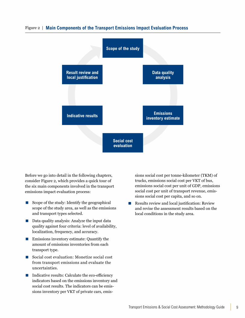
Before we go into detail in the following chapters, consider Figure 2, which provides a quick tour of the six main components involved in the transport emissions impact evaluation process:

▪ Scope of the study: Identify the geographical scope of the study area, as well as the emissions and transport types selected.

▪ Data quality analysis: Analyze the input data quality against four criteria: level of availability, localization, frequency, and accuracy.

▪ Emissions inventory estimate: Quantify the amount of emissions inventories from each transport type.

▪ Social cost evaluation: Monetize social cost from transport emissions and evaluate the uncertainties.

▪ Indicative results: Calculate the eco-efficiency indicators based on the emissions inventory and social cost results. The indicators can be emis-sions inventory per VKT of private cars, emis-

sions social cost per tonne-kilometer (TKM) of trucks, emissions social cost per VKT of bus, emissions social cost per unit of GDP, emissions social cost per unit of transport revenue, emis-sions social cost per capita, and so on.

▪ Results review and local justification: Review and revise the assessment results based on the local conditions in the study area.

Figure 2 | Main Components of the Transport Emissions Impact Evaluation Process

Data quality analysis

Result review and local justification

Emissions inventory estimate

Social cost evaluation

Scope of the study

Indicative results

WRI.org10


METHODOLOGY FRAMEWORK

SECTION II

2.1 Identification of ScopeGeographical scope

Defining a clear geographical boundary before calculating mobile source (transport) emissions is crucial. The guide and tool have a flexible framework that can be used at the country, regional, or city level. It can cover direct emissions in the following geographical areas:

▪ Country’s administrative boundary

▪ Provincial administrative boundary

▪ Regional or cross-boundary (e.g., a cluster of cities or provinces, such as the Yangtze River Delta Region)

▪ City’s administrative boundary

▪ Central urban area

For the city-level emissions estimate, it is common practice to count emissions in the city’s administrative boundary, which covers both the urban built-up area4 and the rural area (WRI, 2015b). However, in most developing counties, a city’s administrative boundary can cover a much wider rural area than such spaces in developed countries. For example, a typical Chinese city, defined by administrative boundary, looks like a huge nonurbanized area embedded with some tiny button-like built-up areas. Within the city’s administrative boundary in most developing

countries, the proportion of the rural area could be huge.

Figure 3 shows a typical layout for a Chinese city. For most cities in China, the built-up area accounts for less than 10% of the entire city administrative area. Even in the most developed Chinese cities (e.g., Shanghai), the built-up area makes up 16% at most. In that case, if one wants to estimate the emissions inventories within a city’s administrative boundary, one has to involve a large portion of freight activities that happen in the city’s suburban and rural areas. This means that air pollutants (especially NOX and PMs) from these freight diesel engines might account for a more significant share than central urban passenger transport modes (e.g., buses, taxis, and private cars).

Note that although intensive human activities happen in the city’s built-up area, most cities’ transport statistics are only available by city administrative level. When users are calculating the city-level transport emissions, I encourage them to be aware of this issue. In order to obtain accurate results, users must be clear on the data scope before using the guide and tool.

Emissions and transport types selection

The guide and tool can help users estimate nine types of emissions from the transport sector,

WRI.org12

including three GHGs and six air pollutants (or criteria air contaminants [CACs]). They are as follows:

▪ GHGs: carbon dioxide (CO2), methane (CH4), and nitrous oxide (N2O).

▪ CACs: nitrogen oxides (NOX), sulfur oxides (SOX), particulate matter less than 2.5 microm-eters in diameter (PM2.5), particulate matter less than 10 micrometers in diameter (PM10), carbon monoxide (CO), and hydrocarbons (HCs).

Although the tool can calculate GHG emissions easily, transport-related air quality issues (in terms of various air pollutants emissions) and their public health and environmental impact to specific local

community are the primary concerns. For GHGs, the guide and tool follow the “scope” defined by WRI’s Global Protocol for Community-Scale Greenhouse Gas Emission Inventories (GPC) and suggest calculating the GHGs for “scope 1, 2, and 3” (WRI, et al., 2014). For other air pollutants, which have more significant local and regional health and environmental impacts rather than global climate impacts,5 the guide and tool only calculate “scope 1” emissions estimate as well as the emissions’ direct local impact within a given geographical boundary. For the next version, WRI will consider including “scope 2 and 3” air pollutants into the guide and tool, which will especially cover indirect emissions from upstream electricity generation and their indirect impact cost.

Figure 3 | City Built-Up Area vs. Admin Area: Typical Chinese City Layout

Note: The dots (built-up area as the percentage of the administrative area) on the right figure are linked to the right (%) y axis.

Sources: Original data from China Statistical Yearbook and China’s Ministry of Housing and Urban-Rural Development..

Urban Area

Suburban & Rural Area

0%

10,000

0

4%

30,000 6%

40,000 8%

50,000 10%

60,000 12%

70,000 14%

80,000 16%

18%90,000

2%

20,000

Chengdu Chongqing Hangzhou

km2

Dalian Qingdao Wuhan Ningbo Suzhou Nanjing Jinan Beijing Shanghai Guangzhou

Built-Up AreaTYPICAL CHINESE CITY LAYOUT

Unban Built-Up Area (km2) City Administrative Area (km2) Built-Up As the Percenage of Admin Area


Scope definitions for city inventories:

• Scope 1: GHG emissions from sources located within the city’s boundary.

• Scope 2: GHG emissions occurring as a consequence of the use of grid-supplied electricity, heat, steam, and/or cooling within the city’s boundary.

• Scope 3: All other GHG emissions that occur outside the city’s boundary as a result of activities taking place within the city’s boundary.

(Sources and boundaries of city GHG emissions)

Scope for transport emissions defined in the GPC:

• Scope 1: Emissions from transportation occurring within the city. This includes all GHG emissions from the transport of people and freight occurring within the city’s boundary.

• Scope 2: Emissions from grid-supplied electricity used in the city for transportation. This includes all GHG emissions from the generation of grid-supplied electricity used for electric-powered vehicles. The amount of electricity used should be assessed at the point of consumption within the city’s boundary.

• Scope 3: Emissions from the portion of transboundary journeys occurring outside the city, and transmission and distribution losses from grid-supplied energy from electric vehicle use. This includes the out-of-city portion of all transboundary GHG emissions from trips that either originate or terminate within the city’s boundary.

Source: WRI, et al., 2014.

Box 1 | “Scopes” Definitions in the GPC

Inventory boundary (including scopes 1, 2 and 3) Geographic city boundary (including scope 1) Grid-supplied energy from a regional grid (scope 2)

industrial processes & product use

in-boundary transportation

stationary fuel combustion

agriculture, forestry & other land use

in-boundary waste & wastewater

out-of-boundary waste & wastewater

out-of-boundary waste & wastewater

transmission & distribution

grid-supplied energy

out-of-boundary transportation

Scope 3

Scope 2

Scope 1

WRI.org14

Transport Emissions Social

Cost

Estimate of transport emissions

Most developing cities and countries have quite diverse types of vehicles (and vessels for waterway transport), especially the vehicles for road freight and the vessels used in inland waterways. The first version of the guide and tool selected 18 transport types that predominate in city or intercity scopes. They include (in alphabetical order) agricultural vehicle, air, bus, e-bike, ferry, inland waterway transport (IWV, including freight and passenger), intercity coach, light rail transit (LRT), metro, military car, motorcycle, private car, railway locomotive (including freight and passenger), taxi, tram, trolley, truck (including heavy-duty truck, medium-duty truck, light-duty truck, and minitruck), and van. These are the most common transport modes in both developing and developed countries. That is why I selected these modes at the first stage.

2.2 Methodology for Emissions In-ventoryTransport emissions inventory can be obtained either through direct air quality monitoring or from estimating the fuel consumed (represented by fuel sold [IPCC, 2006]) or the transport activities (e.g.,

vehicle distance traveled, or tonne-km transported). The different methodologies and approaches to data sources can be grouped in two different categories: top-down and bottom-up (Figure 4).

▪ Top-down approach: based on transport fuel consumption (e.g., fuel sold) and/or direct transport emissions monitoring (e.g., through air quality monitoring and source apportion-ment techniques).

▪ Bottom-up approach: based on transport activi-ties, e.g., vehicle kilometers traveled (VKT).

Both the top-down and the bottom-up approach should be conducted, in parallel, if budget allows. In order to guarantee the quality of emissions inventories, results from both approaches should be compared. Any anomalies between the emissions estimates should be investigated and explained (YCC, 2011). Figure 4 shows a concept flowchart of how to conduct transport emissions estimates by applying both the top-down and the bottom-up approach. By multiplying the emissions amount by the social cost factor (expressed in US$/tonne), researchers can obtain the final result of emissions social cost.

Figure 4 | How to Estimate Transport Emissions Inventories and Social Costs: A Conceptual Flowchart

Note: The methods and equations for the top-down and bottom-up approaches will be detailed in sections 2.1 and 2.2. AQ = air quality.

Top-down: fuel-based for CO2

Top-down: AQ monitoring and source

apportionment

Bottom-up: activity-based for all

emissions

Soical cost factors of emissions


Normally, the top-down and bottom-up approaches apply to both GHG and CAC estimates. In order to obtain the detailed emissions inventories for each transport type, the guide/tool adopts the bottom-up approach, which is based on VKT and other transport activity data (passenger-km or tonne-km transported, aircraft landing and takeoff cycle, vessel activities, etc.). In addition, the tool provides windows for users to enter the data or results from the top-down approach (i.e., data from air quality monitoring, or results directly calculated from fuel consumption). Although the guide/tool mainly focuses on the bottom-up approach, I encourage users to compare top-down and bottom-up results as much as possible. I also encourage users to analyze and interpret the differences in results either quantitatively or qualitatively. In this way, users can make a sound judgment and reach conclusions based on ample evidence.

This guide gives a brief introduction to both the top-down and the bottom-up approach, then details how to use the tool using the bottom-up approach.

2.2.1 Top-down approachThe transport emissions result can be obtained from the top-down approach, which is based on fuel sold and/or air quality monitoring results. Normally, GHG emissions are calculated by “estimating fuel consumption in common energy unit, multiplying by an emission factor” (IPCC, 2000); while CAC emissions are obtained by air quality monitoring and analyzed by source apportionment techniques.6

a. GHG emissions

There are two methods to estimate fuel consumption for transport:

▪ Calculating from energy statistics: Splitting transport fuel data from the total fuel consump-tion item in energy statistics documents.

▪ Conducting a gas station survey: Collecting data on fuel consumed (or sold) from all transport operators (e.g., bus companies, freight compa-nies, taxi companies, airlines, shipping com-panies, private car drivers), and/or from gas stations.

Although the second method could detail into each specific transport type, it might be less feasible (or less comprehensive) in most developing countries because of their weak survey and statistical systems. The first method, however, can be more convenient, because in developing countries energy statistics tend to be more available than other types of information.

The case of China: How to split transport fuel con-sumption from the energy balance sheet?

In China’s existing statistical system (e.g., in the China Statistical Yearbook), a routine item—“total final consumption”7—of the energy balance sheet includes at least the following sectors: (1) “agriculture, forestry, animal husbandry, fisheries, and water conservation”; (2) “industry”; (3) “construction”; (4) “transport, storage, and post”; (5) “wholesale, retail trade and hotel, restaurants”; (6) “other”; and (7) “residential consumption”.8

In China, the “transport, storage and post” sector alone does not necessarily represent the entire transport sector (the mobile source). In fact, most official sources (e.g., the China Statistical Yearbook) only refer to commercial transport types (intercity coach, truck, inland waterway transport, etc.). They do not directly include (YCC, 2011) vehicles owned by private households, enterprises, government, agricultural vehicles, and other special-purpose vehicles that provide noncommercial transport services (e.g., fire trucks). Before the governmental institutional reform that began in 2008, the transport authorities’ statistical system did not even cover urban transport (e.g., taxis and urban public transport), railways and aviation.9 For years, China’s statistical authority has allocated these “outstanding” transport types to the other categories (e.g., in national and local statistical yearbooks, private cars and motorcycles are in the chapter “People’s Living Conditions”, buses and taxis are in the chapter “General Survey of Cities”,10 etc.). These “outstanding” transport types are not always well integrated into the same category (“transport, storage, and post”) within one consistent statistical system. A similar problem occurs in many other developing countries.

In addition, according to the common practice of

WRI.org16

international emissions accounting, “storage” is the stationary source that should not be categorized in the transport (mobile source) sector. In that case, emissions inventory compilers should split the “storage” part from the “transport, storage, and post” category in China’s traditional statistical system.

Because of the above issues, obtaining the mobile source energy-use statistics does not simply entail separating “transport, storage, and post” consumption from the balance sheet. Instead, we

must distill given energy consumption shares from all other sectors or categories mentioned above. These statistics should be combined and accounted for in the entire transport (mobile source) energy consumption.

Table 1 shows what percentage of energy-use from each sector in China’s energy balance sheet should be allocated to transport. This rule was developed through the literature review and expert judgment (Wang, 2006) widely acknowledged by Chinese academia.

SECTOR CATEGORY Adjustment Method*

IAgriculture, forestry, animal husband-ry, fisheries, and water conservantion

Total final consumption: Primary industryGasoline: 97%Diesel: 30%

II Industry (excluding non-energy use) Total final consumption: Secondary industryGasoline: 95%Diesel: 35%

III Construction Total final consumption: Secondary industryGasoline: 95%Diesel: 35%

IV Transport, storage, and post Total final consumption: Tertiary industryAll energy types (excl. 15% of electricity consumption)

VWholesale, retail trade and hotel,

restaurantsTotal final consumption: Tertiary industry

Gasoline: 95%Diesel: 35%

VI Other Total final consumption: Tertiary industryGasoline: 95%Diesel: 35%

VII Residential consumption Total final consumptionGasoline: 100%Diesel: 95%

Table 1 | Transport-Related Energy Use in the Energy Statistics Book: The Case of China

Note: % in this column represents the percentage of the energy allocated for purely transport/mobility use. For example, of all gasoline used in sector “agriculture, forestry, animal husbandry, fisheries, and water conservation”, 97% is transport-related. Note that because the % was estimated by expert judgment only, this approach in the case of China might obtain only rough results.

Sources: (WRI, 2013); in which some data is taken from Wang, 2006.


Figure 5 | Time Trend of Receptor Model Studies in Europe, 2001–2010

b. CAC emissions

Normally, air quality monitoring and source apportionment techniques can help identify CACs’ concentration and sources. Source apportionment is the identification of ambient air pollution sources and the quantification of their contribution to pollution levels. This task can be accomplished using three main approaches: (1) emissions inventories, (2) source-oriented models, and (3) receptor-oriented models (European Commission, 2014; MEP, 2013). The focus of the source apportionment research is on several sources of air pollutants: PM2.5, coarse PM, regulated gaseous pollutants, volatile organic compounds (VOCs), and mercury (USEPA, 2009). According to the European Commission’s Joint Research Center, the receptor models are the best available and most commonly used methodologies for source identification (European Commission, 2014).

There are two key receptor modeling techniques for source apportionment (Figure 5):

▪ Chemical mass balance (CMB): Models that

Note: PCA = principal components analysis; APCA = absolute principal component analysis; FA = factor analysis; APCFA = absolute principal components factor analysis;

PMF-ME = positive matrix factorization—multilinear engine; COPREM = constrained physical receptor model; CMB = chemical mass balance.

Source: European Commission, 2014.

solve the mass balance equation using effective variance least square. These are applied when the number and composition of sources are known (European Commission, 2014).

▪ Positive matrix factorization (PMF): A specific type of factor analytical method that uses exper-imental uncertainty for scaling matrix elements and constrains factor elements to be non-neg-ative (European Commission, 2014). These are applied when the sources are unknown (Envi-ronment and Climate Change Canada, 2013).

However, at present, receptor models have limited capacity to distinguish sources of secondary PM compounds except when combined with elements of source-oriented models and/or other supporting analysis.

Source apportionment (receptor modeling) studies involve the ambient sampling and measurement of atmospheric particles or gases, followed by laboratory analyses to separate and identify the

2001 2002 2003 2004 2005 2006 2007 2008 2009 2010

UNMIX

APCFA

MC

PMF-ME

APCAFA

Lenschow

APEG

PCA

CMB

COPREM

80

70

60

50

40

Num

ber o

f rec

ords

30

20

10

0

WRI.org18

constituents of the samples collected, by their chemical composition. Chemical speciation monitoring helps scientists understand the properties of the airborne pollutants at the receptor site(s) and identify the emission sources, including potential sources not readily identified in preliminary emission inventories, such as cooking fires and airborne particles transported over long distances. Additionally, the analyses help quantify the contribution of known emissions sources and can help validate and improve the emissions inventory itself.

Successful application of source apportionment (receptor modeling) methods and support to effective policymaking and decision-making depends on the accuracy and relevance of the air quality measurements and the interpretations made by the scientist and air quality manager.

A detailed explanation of CMB and PMF is given in Environment and Climate Change Canada, 2013.

2.2.2 Bottom-up approachFollowing the recommendation of the Intergovernmental Panel on Climate Change in 2006 IPCC Guidelines for National Greenhouse Gas Inventories (IPCC, 2006), “if distance traveled data are available, it is good practice to estimate fuel use from the distance traveled data”. In most cases, including estimating CACs, the bottom-up approach follows such driving activity–based methodology, using vehicle kilometers traveled (VKT) as the most primary activity data. In order to calculate the detailed transport emissions inventories and the associated social costs, the guide and tool adopt the equations as follows:

Energy demand = ∑i,j [Vehiclei,j × Activityi,j × FEi,j]

Emission = Energy demandi,j × EFi,j,k

ESC = ∑i,kEmissioni,j,k×SCFk

where,• ESC (US$) = emissions social cost (of transport);11

• Emission (tonne) = emission amount by weight, e.g., tonnes of CO2 or PM2.5;

• SCF (US$/tonne) = social cost factor of emissions;

• Energy demand (e.g., l, tce; or kWh) = total

energy use estimated from the activity data;• EF (e.g., g/l, t/tce, or g/km) = emission factor;• Vehicle = number of vehicles (or vessels, etc.) of

type i on fuel j;• Activity (e.g., VKT, TKM, PKM) = annual activity

performed (e.g., distance traveled/VKT, tonne-km, or passenger-km transported) per vehicle of type i on fuel j;

• FE (e.g., l/100km, or l/100TKM) = fuel efficiency: average fuel consumption per unit of activity performed by vehicles of type i on fuel j;

• i = vehicle or vessel type (e.g., truck, bus);• j = fuel type (e.g., gasoline, diesel, NG); and• k = emission type (e.g., CO2, PM2.5).

The United States Environmental Protection Agency (USEPA) also defines a general equation for emissions estimation (USEPA, 2015b). If the policymakers and decision-makers want to consider the effect of emissions reduction measures, they can use the USEPA’s equation as follows:

E = A×EF×(1-ER/100), where,E = emission; A = activity rate; EF = emission factor; ER = overall emissions reduction efficiency (%).

The bottom-up equation parameters can be broken down into more detailed inputs. Interpretations of each primary input and data collection method are detailed in Chapter 4.

▪ Vehicle number: Number of vehicles by vehicle type, such as agricultural vehicle, aircraft, bus, e-bike, ferry, intercity coach, inland waterway transport (IWV, including freight and passen-ger), light rail transit (LRT), metro, military car, motorcycle, private car, railway locomotive (including freight and passenger), taxi, tram, trolley, and truck (including light-, medium-, and heavy-duty, and well as minitruck), and van; by fuel type, such as diesel, dual fuel, elec-tric, gasoline, hybrid, liquefied petroleum gas (LPG), natural gas (NG), crude oil, kerosene, and average; and by emission standard, such as Euro I–V and pre-Euro.

▪ Activity: Activity data by vehicle type, such as vehicle kilometers traveled (VKT), passenger-kilometers (PKM) traveled, tonne-kilometers (TKM) traveled, total passenger time, aircraft landing and takeoff (LTO) cycle.


▪ Traffic: Trip split or driving conditions split by vehicle type, such as trip % (for city driv-ing, rural driving, and highway driving), speed (km/h for peak, off-peak, and average), peak hours per day.

▪ Fuel efficiency (FE): FE by vehicle type and fuel type under given driving conditions (in l/100km, l/100PKM, l/100TKM, m3/100km, kgce/100TKM, kWh/100PKM, etc.), for ex-ample, l/100km for a diesel bus for city driving under 30km/h.

▪ Emission factor (EF) for GHGs: EFGHG by fuel type in local and default data (in tCO2e/l, or tonne/l, or tonne/kWh, etc.), for example, tCO2e emissions per liter of gasoline.

▪ Emission factors for CACs: EFCAC by vehicle type, fuel type and emission standard under given driving conditions, in local and default data (in g/km, or g/kg, g/LTO); for example, g/km PM2.5 for a diesel bus (Euro III) for city driv-ing under 30 km/h.

▪ Social cost factor (SCF) of emissions: SCF by emission type, such as CO2, CH4, N2O, PM10, PM2.5, NOX, SOX, CO, and HC (in US$/tonne).

2.2.3 Explanation of gapsAs mentioned, if time and budget allow, users are encouraged to use different approaches (bottom-up and top-down) or techniques to estimate the emissions inventory and the source apportionment. It is a good practice to compare the results from the different approaches and techniques. Through this cross-verification procedure, gaps of the results will be properly investigated and explained. Finally, the results should be justified or recalculated. Figure 6 shows a concept flowchart for the gap analysis.

Here I recommend some simple judgments when comparing the results: If the gap of the results is under 5%, I assume the difference can be accepted; if it is between 5% and 10%, the difference will have to be explained and the results weighted; if it is above 10–15%, I assume that the difference is “significant” (unacceptable) and needs further explanation and recalculation. However, in reality, in many cases, the gap could be more than 15%. In that case, I recommend the following steps:

▪ Use the official data (e.g., energy statistics) to calculate emissions.

WRI.org20

▪ List the results from other approaches, for ex-ample, by comparing the results from top-down and bottom-up approaches.

▪ Analyze the reasons for the deviations and pro-vide explanations (if possible).

As in Figure 6, significant gaps in results between different approaches or technologies stem from three types of errors: (1) systematic errors, (2) calculation errors, and (3) unknown reasons. Most systematic and calculation errors can be corrected and/or explained. Table 2 shows some typical reasons for systematic errors and suggests how to resolve the problems.

In addition to the gaps between different ap-

Figure 6 | Conceptual Flowchart for Gap Analysis

proaches or techniques, there are some uncertain-ties in the calculation. These result, for example, from the commonly low quality (in terms of availability, accuracy, frequency, and localization) of activity data in developing countries, as well as from the weak localization of fuel efficiency data and emission factors, and weak representativeness of the default data. All these uncertainties might reduce the robustness of the estimate. In addition to evaluating the quality of the input data, I en-courage users to include quality assurance/quality control (QA/QC) processes as follows to minimize uncertainty. The sources for our QA/QC are IPCC (2006) and YCC (2011).

▪ “Comparison of emissions using alternative approaches: The inventory compiler should

Gap analysis Calculation error Examine & recalculate

Significant Explain & recalculate

Significant Recalcuate

Insignificant Explain & use the weighted average value

Insignificant Use the weighted average value

Reason unknown

Systematic error


compare estimates using both the fuel statistics and VKT data (top-down and bottom-up ap-proaches). Any anomalies between the emission estimates should be investigated and explained. The results of such comparisons should be re-corded for internal documentation. Revising the following assumptions could narrow a detected gap between the approaches:

• Off-road/non-transportation fuel uses

• Annual average vehicle mileage

• Vehicle fuel efficiency

• Vehicle breakdowns by type, technology, age, and so on

• Use of oxygenates/biofuels/other additives

• Fuel use statistics

• Fuel sold/used

▪ Review of emission factors: If default emission factors are used, the inventory compilers should

SYSTEMATIC ERRORS TYPICAL REASONS/INTERPRETATIONS Solutions

Top-down vs. bottom-upTop-down approach covers more fleet than bottom-up approach (e.g., fleet for all commercial, military, and private use).

Make sure the inventory covers all types of fleet, especially the private fleet and the off-road mobile sources.

Top-down approach might cover non-mobile sources (e.g., “storage” in China’s case).

Try to delete the non-mobile sources from the inventory.

Different AQ monitoring & source ap-portionment techniques

Some results do not include secondary sources.

Try to include the secondary source analysis in the study.

Uncertainty of EFs and SCFsLack of localization; the existing study in the literature is weak.

More localization activities, e.g., local testing, surveys, local expert judg-ment, literature reviews, local statistic reviews, etc.

Table 2 | Typical Reasons for Systematic Error and the Solutions

ensure that they are applicable and relevant to the categories. If possible, the default factors should be compared to local data to provide fur-ther indication that the factors are applicable.

▪ Activity data check: The inventory compiler should review the source of the activity data to ensure applicability and relevance to the cat-egory. Where possible, the inventory compiler should compare the data to historical activity data or model outputs to detect possible anoma-lies. The compiler ensure the reliability of activ-ity data regarding fuels with minor distribution; fuel used for other purposes, on- and off-road traffic, and illegal transport of fuel in or out of the study area. The inventory compiler should also avoid double counting of agricultural and off-road vehicles.

▪ External review: The inventory compiler should perform an independent, objective review of the calculations, assumptions, and documentation of the emissions inventory to

WRI.org22

assess the effectiveness of the QA/QC pro-gram. The peer review should be performed by expert(s) who are familiar with the source category and who understand the inventory re-quirements. The development of CH4 and N2O (and most CAC) emission factors is particularly important because of the large uncertainties in the default factors.”

2.3 Methodology for Social Cost EvaluationAs with the emissions inventory assessment, evalu-ation of the social cost of mobile source emissions is performed using top-down and bottom-up approaches. According to Ricardo-AEA’s report, Update of the Handbook on External Costs of Transport (Ricardo-AEA, 2014), each approach has the following features:

▪ “Bottom-up approach: The estimate of mar-ginal costs is usually based on bottom-up ap-proaches considering specific traffic conditions and referring to case studies. They are more

precise and accurate, with potential for differen-tiation. However, the estimation approaches are costly and difficult to aggregate (e.g., to define representative average figures for typical trans-port clusters or national averages).

▪ Top-down approach: Top-down approaches using average national data are applied. Such approaches are more representative on a gen-eral level, allowing also a comparison between modes. However, the cost function has to be simplified and cost allocation to specific traf-fic situations and the differentiation for vehicle categories is rather rough.”

The bottom-up and top-down approaches are equally important, though each has pros and cons mentioned above. The top-down approach is much easier and quicker for developing coun-tries with limited budgets, but it could have much larger uncertainties, so that the final results are often debated among researchers and decision-makers. The bottom-up approach, in contrast, could give more accurate results, but the costs in time, budget, and human resources can be huge.


According to Ricardo-AEA (2014), “the existing literature for efficient pricing mainly recommends a bottom-up approach following the impact pathway approach (IPA) methodology. In prac-tice, however, a mixture of bottom-up and top-down approaches (with representative data) can be observed. Most important is the definition of appropriate clusters with similar cost levels (such as air pollution levels, traffic characteristics, and population density).”

In this section, I have introduced the basic framework of the bottom-up (e.g., IPA) and top-down approach-es. Because of the complexity and cost of the bottom-up approach, I recommend that researchers in devel-oping countries use the top-down approach (based on the average cost values) at first. But in the long run, developing countries should encourage more case studies that follow a bottom-up approach (based on marginal cost values) and summarize results and experiences, especially for countries still having ex-tremely limited cases. The detailed introduction of the social cost factor (as the average cost value) from the top-down approach is explained in Section 4.7.

2.3.1 Definition of social cost of emissionsThe social cost represents the sum of the private (internal) and external costs (Iannone, 2012; Coase, 1960; Prud’homme, 2001; Nash, 2003; European Commission, 2008; Ricardo-AEA, 2014; Song, 2014a). Some studies have specially defined the social cost as the sum of the external costs that are not internalized. Social cost in transport sector includes environmental costs (emissions, noise, other types of pollutants), congestion costs, acci-dent costs (Ozbay, et al., 2007), and climate change costs. Emissions constitute the most important pol-lution type for the transport sector; and the major-ity of the external costs from transport-related air pollution arise through the effects on human health (Ricardo-AEA, 2014). This guide, therefore, refers to social cost as the external cost from transport emissions, and mainly focuses on the impact on public health.

How should we define the social cost of emissions? Definition of the social cost of carbon (SCC) can be a good example. SCC is a common type of emis-sions social cost and is often used to evaluate the

WRI.org24

external cost by carbon emissions. The USEPA defines SCC as a widely applied instrument for cost-benefit analysis (CBA) during decision-mak-ing. “It allows agencies to incorporate the social benefits of reducing CO2 emissions into CBA of regulatory actions that have ‘marginal’ impacts on cumulative global emissions. The SCC is an esti-mate of the monetized damages associated with an incremental increase in carbon emissions in a given year. It is intended to include (but is not limited to) changes in net agricultural productivity, human health, property damages from increased flood risk, and the value of ecosystem services due to climate change” (USEPA, 2010; USEPA, 2016c). Definitions of the social cost of other types of air pollutants (CACs) are similar to the definition of SCC. However, CACs could have large different

impacts from GHGs, especially in terms of public health and impact scale. Therefore, the social cost quantification of CACs might be more complicated and contain large uncertainties. Different from GHGs that have long-term (100 years or more) and global-scale impacts on climate, environment, and human life, some CACs (e.g., PM2.5) have short-term (e.g., decades or less) (ICCT, 2009) and smaller-scale impacts on air quality at the regional or local level (e.g., mostly on human health and the ecosystem at the city or city-cluster scale, etc.). Although the atmospheric lifetime of some CACs (e.g., black carbon) might be much shorter than GHGs (black carbon stays in the atmosphere for only several days to weeks, whereas CO2 has an atmospheric lifetime of more than 100 years) (Ra-manathan & Carmichael, 2008), their impacts on regional or local level public health, environment, and short-term climate could be fatal, especially on human health because of air quality degrada-tion. Some short-lived climate pollutants (SLCPs) (CCAC, 2016),12 such as black carbon (BC) in PM2.5, may not only damage human health but also create strong temporal radiative forcing to substantially change regional climate (e.g., ice melting, regional temperature, and rainfall), and eventually global climate (ICCT, 2009). The transport sector is be-coming the leading source of BC.

Black carbon sources in developing and devel-oped countries are substantially different (USEPA, 2015c). But in general, fossil fuel combustion in transport (especially mobile source diesel engines), solid biofuel combustion in residential heating and cooking, and open biomass burning from forest fires and controlled agricultural fires are the sourc-es of about 85% of global black carbon emissions (ICCT, 2009). Although residential heating and cooking are the main contributors to black carbon emissions in the developing world, mobile source emissions will soon become predominant because of the strong urbanization and motorization trend in some fast-developing countries (e.g., China). In that case, all the social impacts (including the costs to public health, climate, and the environment) from transport sources need to be noted and well quantified.

2.3.2 Bottom-up approachAlthough the estimate of external costs has to con-sider several uncertainties, there is wide consensus


Box 2 | Impacts of Black Carbon

Chemically, black carbon is a component of fine particulate matter (PM2.5

). Black carbon consists of pure carbon in several linked forms (Anenberg, et al., 2012). It is formed by incomplete combustion of fossil fuels, biofuels, and biomass (USEPA, 2015c). It is emitted in both anthropogenic and naturally occurring soot. Black carbon is the most effective form of PM, by mass, at absorbing solar energy: per unit of mass in the atmosphere, black carbon can absorb a million times more energy than CO

2 (USEPA, 2015c). According to the

IPCC, black carbon is the third largest contributor to the positive radiative forcing that causes climate change. When emitted into the atmosphere and deposited on ice or snow, black carbon causes global temperature change, melting of snow and ice, and changes in precipitation patterns (ICCT, 2009). In addition, PM is the most harmful to public health of all air pollutants. Black carbon PM contains very fine carcinogens and is therefore particularly harmful. It is estimated that from 640,000 to 4,900,000 premature human deaths could be prevented each year by utilizing available mitigation measures to reduce black carbon in the atmosphere (Weinhold, 2012). Controls on black carbon (and the other SLCPs) thus can bring rapid regional and local and global climate benefits (ICCT, 2009), as well as public health and other co-benefits.

Climate Effects:Black carbon (BC) influences climate by (1) directly absorbing light; (2) reducing the reflectivity (“albedo”) of snow and ice through deposition; and (3) interacting with clouds. Through these mechanisms, BC has been linked to a range of climate impacts, including increased temperatures and accelerated ice and snow melt. Sensitive regions such as the Arctic and the Himalayas are particularly vulnerable to the warming and melting effects of BC. BC also contributes to surface dimming, the formation of atmospheric brown clouds (ABCs), and changes in the pattern and intensity of precipitation. Reducing current emissions of BC may help slow the near-term rate of climate change, particularly in sensitive regions such as the Arctic. BC’s short atmospheric lifetime (days to weeks), combined with its strong warming potential, means that targeted strategies to reduce BC emissions can be expected to provide climate benefits within the next several decades.

Public Health Effects:BC contributes to adverse impacts on human health, ecosystems, and visibility associated with ambient fine particles (PM

2.5). Short-term

and long-term exposures to PM2.5

are associated with a broad range of human health impacts, including respiratory and cardiovascular effects as well as premature death. Over the past decade, the scientific community has focused increasingly on trying to identify the health impacts of particular PM

2.5 constituents, such as BC. However, there currently is insufficient information to differentiate the health effects

of these constituents; thus, the USEPA assumes that many constituents are associated with adverse health impacts. The limited scientific evidence currently available about the health effects of BC is generally consistent with the general PM

2.5 health literature, with the most

consistent evidence for cardiovascular effects. In the United States, the average public health benefits associated with reducing directly emitted PM

2.5 are estimated to range from $290,000 to $1.2 million per tonne of PM

2.5 in 2030. The cost of the controls necessary to achieve

these reductions is generally far lower. Globally, PM2.5

, both ambient and indoor, is estimated to result in millions of premature deaths worldwide, the majority of which occur in developing countries.

Environmental Effects:PM

2.5, including BC, is linked to adverse impacts on ecosystems, to visibility impairment, to reduced agricultural production in some parts of the

world, and to materials soiling and damage.

Source: USEPA, 2016b.

WRI.org26

on the major methodological issues (Ricardo-AEA, 2014). For evaluating transport-related air pollu-tion cost, the impact pathway approach (IPA), or damage cost approach, is broadly acknowledged as the preferred methodology, and is officially used in Europe. The IPA is a bottom-up approach that integrates the state-of-the-art knowledge in different scientific disciplines13 in a common and coherent framework (Mayeres, et al., 2001). Box 3 introduces the five steps of the IPA. It follows a logical, stepwise progression from pollutant emis-sions to the determination of impacts and subse-quently the quantification of economic damage in monetary terms (Ricardo-AEA, 2014). The final step, “damage” is the crucial step where the selec-tion of quantification methods is based on different cost components (Table 3). For example, “will-ingness to pay” (WTP) is selected for evaluating health damages; the “abatement cost approach” is selected for climate change. In addition to the IPA, research bodies can refer to the USEPA’s Environ-mental Benefits Mapping and Analysis Program (BenMAP) (USEPA, 2016a), which is commonly used in the United States, during evaluation works

(see Box 4). Both the United States and the Euro-pean Union have rich experience in quantifying the health impacts of air pollutant emissions. The key component for evaluating health impacts (as the most typical social cost) from transport emissions is to consider (1) the population being affected and (2) the damages in monetary form. According to the USEPA, the health impact cost should be evalu-ated using both “Cost of Illness” and “Willingness to Pay” metrics: “The Cost of Illness metric sum-marizes the expenses that an individual must bear for air pollution–related hospital admissions, visits to the emergency department and other outcomes; this metric includes the value of medical expenses and lost work, but not the value that individuals place on pain and suffering associated with the event. By contrast, Willingness to Pay metrics are understood to account for the direct costs noted above as well as the value that individuals place on pain and suffering, loss of satisfaction and leisure time” (USEPA, 2015a). However, in many coun-tries, only limited studies focus on the social cost of transport emissions, and there may be signifi-cant uncertainty in the results.

COST COMPONENT BEST PRACTICE APPROACH

Human healthIPA framework: evaluating health impact cost using WTP or WTA approach; or using “cost of illness” and “opportunity cost” approach (including VSL, medical expenses, lost work).

Infrastructure/material damages IPA framework: repair costs.

Nature and landscapeIPA framework: cost of losses (e.g., market price and non-market value of crop); compensation cost approach (based on virtual repair cost).

Climate changeAvoidance cost approach (based on GHG emissions reduction scenarios) or damage cost approach; shadow price of emission trading system.

Table 3 | Best Practice Valuation Approaches for Air Pollution Cost Components

Sources: Adapted from Ricardo-AEA, 2014.


Box 3 | Impact Pathway Approach (IPA)

The Impact Pathway Approach (IPA), is one of the most important outcomes of the European Union’s External Costs of Energy (ExternE), a program package that lasted from the 1990s to 2005. The IPA is used to estimate monetary values of the negative external cost of emissions. The IPA has been widely adopted, and further improved, by researchers and decision-makers and is considered to be one of the most reliable instruments for quantifying the negative environmental cost of emissions.

The IPA framework includes five steps: (1) emissions; (2) dispersion; (3) exposure; (4) impacts; and (5) damage.

• Step 1 Emission: Identify emission sources; estimate the amount of pollutants through applying transport emission model or emission factors. The amount is usually presented in pollutant mass (e.g., kilogram of PM

2.5).

• Step 2 Dispersion: Simulate pathway of pollutant dispersion around emission sources through air pollutant monitoring and applying atmospheric dispersion models. The scenario of pollutant dispersion is difficult to build; the data accessibility is low. The level of air pollution dispersion is often expressed in concentration (e.g., µg/m3).

• Step 3 Exposure: The impacts of transport air pollutant emissions are highly location-specific and depend on many factors, such as local traffic conditions. The exposure assessment therefore relates to the population and the ecosystem being exposed to the air pollutant emissions. Spatially detailed information (e.g., in the GIS) on population density and the geographical distribution of the ecosystem must be available to allow proper assessment.

• Step 4 Impacts: The impacts caused by the emissions are determined by applying so-called exposure-response functions that relate changes in human health and other environmental damages to unit changes in ambient concentrations of pollutants. These exposure-response relations are based on epidemiological studies. The relationship is often expressed in equations, such as “increased PM

2.5 emissions (µg/m3)

=> cases of asthma”.

• Step 5 Damage (Cost): The impact of the emissions on humans and the ecosystem must be evaluated and transformed into monetary values. This step is often based on valuation studies assessing, such as the willingness to pay (WTP) for reduced health risks. This is the external cost that is often expressed in forms such as US$ or other types of currency.

Source: European Commission, 2005; Ricardo-AEA, 2014; Mayeres, et al., 2001; ExternE, 2014.

TOOLS

Emission models/inventories

Dispersiom modelslocal, regional

Exposure assessmentGIS based info on receptors at risk

Market prices“Willimgness to Pay”-studies

Exposure-Response relationshipspublic healthagriculturematerials

ecosystems

Critical loads

STEPS

EMISSIONS

DISPERSION

EXPOSURE

IMPACTS

DAMAGE

IMPACT

EXPOSURE

SOURCE(specification of site and technology)

---------------------------------------------------⇒ emission

(e.g., kg/yr of particulates)

DISPERSION(e.g. atmospheric dispersion model)

---------------------------------------------------⇒ increase in concentration at receptor sites

(e.g., μg/m3 of particulates in all affected regions)

MONETARY VALUATION---------------------------------------------------

⇒ cost (e.g., cost of asthma)

DOSE-RESPONSE FUNCTION(or concentration-response function)

---------------------------------------------------⇒ impact

(e.g., cases of asthma due to ambient concentration of particulates)

Does-Response Function

DOSE

WRI.org28

The Environmental Benefits Mapping and Analysis Program (BenMAP), developed by the USEPA, is an open-source computer program that calculates the number and economic value of air pollution–related deaths and illnesses. The software incorporates a database that includes many of the concentration-response relationships, population files, and health and economic data needed to quantify these impacts.

BenMAP is composed of the following functions:

• Estimating health impacts:The health impact function incorporates four key sources of data: (1) modeled or monitored air quality changes; (2) population; (3) baseline incidence rates; and (4) an effect estimate. With the above four groups of data the function is able to estimate the population impacted and the level of impact.

• Evaluating the economic value of health impacts:The program calculates the monetary values of health damages using both “Cost of Illness” and “Willingness to Pay” metrics. “The Cost of Illness metric summarizes the expenses that an individual must bear for air pollution–related hospital admissions, visits to the emergency department and other outcomes; this metric includes the value of medical expenses and lost work, but not the value that individuals place on pain and suffering associated with the event. By contrast, Willingness to Pay metrics are understood to account for the direct costs noted above as well as the value that individuals place on pain and suffering, loss of satisfaction and leisure time” (USEPA, 2015a).

Source: USEPA, 2016b.

Box 4 | Environmental Benefits Mapping and Analysis Program (BenMAP)

An air auality policy reduces the number of hospital

admissions by 100

The economic value of each avoided admission is

$5,000 in the year 2010

$5,000/admission 100•$5,000 = admission

The economic value is the number of cases multiplied by the value of each admission

Steps to Calculating Health Impacts

Note:- △Y: health effects change of certain type health effects terminal, such as the excessive number of illness or the number of deaths;- Y0: the baseline condition of certain type health effects terminal, such as baseline morbidity or mortality;- POP: exposed population;- β: the relationship coefficient between the health risk of certain type health effects terminal and atmospheric particulate matter concentration, namely dose-response coefficient of relationship;- △PM: the difference between the value of atmospheric particulate matter concentration estimated and the value of the reference concentration used in the evaluation.

△Y=Yo(1-e-β△PM)*Pop

(-β)

Effect estimate

Pollutant change Population Baseline incidence

Healthimpact

(△PM)

(△Y)

(Pop) (Yo)


2.3.3 Top-down approachIf time and budget for a bottom-up approach (e.g., through the IPA) are limited, I encourage re-searchers to use top-down approaches to calculate emissions social cost using average national-level or regional-level social cost factors (SCFs). Such approaches are more representative on a general level, allowing comparison between modes. Al-though there might be a high uncertainty in social cost (e.g., cost of health impact) quantification, it is common practice to conduct meta-analysis (Greenland & O’Rourke, 2008), that is, to review great numbers of previous studies to obtain com-paratively statistical robust aggregated SCFs (in $/tonne), and then localize SCFs through “value transfer” techniques introduced by Navrud (2009); Navrud (2004); and (Navrud & Ready, 2007). The social cost, therefore, can be estimated by multi-plying SCF by the amount of air pollutants. This is deemed the simplest and most efficient way to evaluate social cost.

As a key input parameter for the social cost evalu-ation, SCFs measure the total social cost of unit mass pollutant within specified geographical boundaries. As mentioned above, researchers can refer to existing SCFs of other countries if sources for developing own SCF are limited, and transfer/localize the values if possible. Unlike the IPA, which follows the bottom-up pathway, estimation using SCF (also widely adopted) is a top-down method. The equation is as follows:

ESC = ∑i,j(Emissioni,j × SCF)

where,• ESC = emissions social cost ($);• Emission = amount of emission (tonne);• SCF = social cost factor ($/tonne);• i = type of emission source• j = type of atmospheric emissions

A detailed explanation of SCFs input and its uncer-tainties is presented in Chapter 4.

2.3.4 Application of social cost evaluationThe importance of social cost evaluation is to help decision-makers conduct social cost-benefit analy-sis (SCBA)14 on emissions reduction technologies or policies, therefore securing the most cost-efficient

policy or technology options (e.g., options with net present value of >0). The evaluation requires con-sideration of total social welfare as a whole, that is, social costs and benefits to the entire population or community, rather than internal costs and benefits for individual groups. However, little policymaking on transport-related environmental protection is based on mature SCBA. The lack of SCBA, com-mon in many developing countries’ policymaking and assessment, may be due to a lack of aware-ness, weak legislation and institutional set-up, and poor data transparency and quality. Social cost evaluation is urgently needed to identify damages of emissions (or other forms of pollution) and to develop policies. Benefits (or co-benefits) in this context are the comprehensive sum of all external costs reduced from the implementation of emis-sions reduction policies or technologies.

WRI.org30


DATA QUALITY

15

SECTION III

Most developing countries/cities have limited official statistical

data accessible to the general public, especially detailed transport

activity data.16 Although some data are available from official

sources, they are sometimes not presented in a regular manner and

their accuracy is suspect. In some developing countries, the data

are incomplete and unreliable.17 This section presents an example of

China’s data sources and its data quality.

WRI.org32

When estimating transport emissions inventories in developing countries and cities, the guide and tool encourage users to always conduct data source scanning and data quality analysis.

3.1 Data Sources: The Case of ChinaThe problems in China’s data and statistics system stem from (1) low efficient coordination among governmental departments with different jurisdictions; (2) inconsistent data collection and statistics reporting protocols; (3) immature statistics system and statistical methodologies; (4) possible data manipulation; and (5) weak information transparency. In fact, the data reporting system, data consistency and accuracy, and the transparency of the statistics data (transparency among government departments and between the government and the public) could be key reasons for the poor emissions estimation.

Currently, at least six national-level departments oversee different aspects of the transport sector

in China. They are (1) the Ministry of Transport (MOT) for urban and intercity commercial transport operation (i.e., intercity coach, truck, bus, taxi, rail, tram/trolley, civil aviation, inland waterway, and maritime transport); (2) the Ministry of Housing and Urban-Rural Development (MOHURD) for urban transport infrastructure construction; (3) the Ministry of Public Security (MPS) for vehicle registration; (4) the Ministry of Environmental Protection (MEP) for transport pollutant emissions management and other relevant environmental issues; (5) the Ministry of Industry and Information Technology (MIIT) for vehicle technical standards (e.g., fuel economy) and manufacture (e.g., production admission); and (6) the National Development and Reform Commission (NDRC) for general supervision of logistics, prices/subsidies, infrastructures, energy, and climate change issues (e.g., GHG emissions). Like national-level governments, local governments have their own diversified hierarchies and fragmented jurisdictions in the transport sector (WRI, 2015a). They also have problems of coordination and inconsistent statistic systems. All these governmental departments (as well as their affiliated research institutes) hold their own statistics and the basic data relevant to transport emissions and impact evaluations. Unfortunately, their data collection mechanism and statistics systems have not been well integrated or coordinated.

Although there are limitations in China’s statistics system, I encourage users to use data from the open official sources as much as possible. Like most tools, our guide and tool prefer official and localized data over unauthorized and general or default data. The input data follow this order of priority: official or authorized sources, surveys with significant samples, interviews and expert judgment, gray literature, and default data (general data). Table 4 provides some key sources for the primary data input for the guide and tool. It is also worth mentioning that in the era of big data, using real-time big data from the various means of modern facilities (data from vehicle GPS, vessel automatic identification system [AIS], satellite sensor, mobile phone, private or public mobility service platforms such as Uber, etc.) will be the way of the near future.

3.2 Data Quality AnalysisTransport emissions estimation methodology itself is neither overly complicated nor difficult. The key barriers in the estimation process in most developing


DATA UNIT KEY SOURCES AND NOTE

Vehicle number setPublic security authorities18 (for all vehicles); commercial transport operators (e.g., bus/shipping companies); transport authorities (for commercially used vehicles); statistical authorities; big data providers.

VKT km

Commercial transport operators (e.g., bus/taxi/shipping companies); public survey (for private vehicles); public security authorities (for all vehicles); transport demand forecast model; 4S chain store; big data providers.

PKM PKMCommercial transport operators (e.g., bus companies); transport authorities; transport associations; statistical authorities; big data providers.

TKM TKMCommercial transport operators (e.g., freight companies); transport authorities; transport associations; statistical authorities; big data providers.

Driving conditions split kmCommercial transport operators (e.g., bus/shipping companies); public survey (for private vehicles); local governments and transport authorities; big data providers.

Speed km/hCommercial transport operators (e.g., bus/shipping companies); public survey (for private vehicles); public security authorities (for all vehicles); local governments; transport authorities; big data providers.

Fuel efficiencyl/100km, l/100PKM, or

l/100TKM

Commercial transport operators (e.g., bus/shipping companies); public survey (for private vehicles); auto/vessel makers; transport authorities; transport associations; statistical authorities; big data providers.

Emission factors for GHGs

t/tce, or t/lERI; NDRC; IPCC, environmental exchange center, local governments; research institutes; energy authorities.

Emission factors for CACs

g/km or g/lVECC/MEP; local environmental protection authorities; local governments; research institutes.

Social cost factors US$/tWide range of literature; research institutes; CDC; WHO; sophisticated public survey; big data providers.

Top-down fuel consump-tion

tce

Commercial transport operators (e.g., bus/shipping companies); transport authorities; statistical authorities; local governments; public survey (for private vehicles); gas stations; energy departments; big data providers.

Top-down emissions tNDRC; local DRC; MEP, NASA, local EPB; research institutes; transport authorities; big data providers.

Table 4 | Key Sources of Primary Data: The Case of China

WRI.org34

countries and cities are the data issues, such as unavailability of data (especially activity data like VKT) and weak data quality (e.g., a sample is not representative/significant; data are not accurate, reliable, or consistent, etc.). There are some typical data (and statistics system) problems in both the top-down and bottom-up approaches:

▪ Problems in the top-down approach: (1) Some official data sources (e.g., the annual statistical yearbook) do not cover and/or disag-gregate all types of transport. For example, in China, “total fuel consumption” under the category “transport, storage, and post” does not cover noncommercial transport means, such as vehicles belonging to enterprises and pri-vate households, agricultural vehicles, military vehicles, other special-purpose vehicles that provide noncommercial transport services (e.g., fire trucks), and so on. Oddly, it covers “stor-age” that does not belong to the mobile sources (transport). (2) Fuel consumption data collected

from gas stations (if available) are not split by vehicle type.

▪ Problems in the bottom-up approach: (1) VKT data are absent in almost all official sources in many countries, especially the VKT for private cars. (2) Statistical estimates are not significant because of the unrepresenta-tive small sample size and extremely diversi-fied vehicle types in developing countries. This problem could be even more severe for data collection in intercity freight transport, where authorities only collect activity data from big and medium-sized companies. Unfortunately in the case of China, these big and medium-sized companies account for an insignificant share, while small trucking companies with fewer than 10 trucks account for more than 90% of China’s trucking market (MOT, 2013). (3) Many coun-tries and cities do not have their own localized emission factor database. This is probably the main reason for the big uncertainties in emis-sion estimates in developing areas.

Figure 7 is a concept map that presents the level of quality and level of localization of data in developing countries/cities. Generally, in most developing countries and cities, the “vehicles number” has the best quality. The data are normally collected in full sample size, having good localization and a high level of availability, accuracy, and regular collection and reporting. The emission’s “social cost factor” (SCF) has the poorest quality, while the data are the least available, least accurate, and least regularly collected and reported. In addition, it lacks a localization process, meaning one often cannot find the SCF data (or have the relevant studies on SCF) for specific cities in developing countries.

How to evaluate data quality?

The YCC Transport & Climate Change Center (YCC, 2015) has been conducting a large-scale data mapping and data quality diagnosis during its transport emissions estimation for 17 Chinese cities since 2011 (YCC, 2011). It developed the “data quality diamond” to assess the quality of the existing data required for transport emissions equations. As shown in Figure 8, different colored lines on the “diamond” represent data for different parameters in the emissions equation (vehicle numbers, VKT, fuel efficiency, emission factor, etc.) for different transport


Figure 7 | Level of Quality and Localization of Data in Developing Countries

Note: This graph only presents a concept diagnosis of the data quality. It compares the quality of each parameter or data point in a qualitative and relative way. The relative position of each parameter or data point on this coordinate and the comparative size of data representativeness are determined by expert judgment.

1. “Availability”, “accuracy”, and “frequency” represent the quality of the data in the guide and tool.

2. The “level of localization” shows if the data are well localized in the study area (for example, if one can get the “SCF” data for Shanghai or just general/average data for Asia).

3. The size of each data dot represents the sample size of the data. Larger dots indicate that the data sample is more statistically representative or significant (for example, “vehicle number” is the full sample data, which means it has the biggest dot size).

Vehicle number

Best availability, accuracy, and

frequency

Worst availability, accuracy, and frequency

Most localized

Least localized

Level of Quality

Level of Localization

Trip split

Speed

VKT

FE

TKM

SCF

PKM

EFGHG

EFCAC

WRI.org36

Figure 8 | Data Quality Diamond: A Concept Chart for Data Quality Assessment

Note: This is a concept chart to demonstrate the idea that for each data point (e.g., VKT, emission factor), represented by a different colored line, the quality can be assessed by four indicators—availability, accuracy, frequency, and localization. The score for each data quality ranges from 0 to 10, where 0 = worst data quality and 10 = best data quality.

1. Availability: score from 0 to 10, where 0 = data do not exist or were not collected; 1 = worst availability (e.g., data only available to a small authorized group and confidential to the public; data only partially available or only appear in certain reports/speeches/PowerPoint/webpages instead of in open statistical documents, etc.); and 10 = best availability (e.g., data published online and free to the general public; always appear in the statistical documents, etc.).

2. Accuracy: score from 0 to 10, where 0 = data do not exist or were not collected; 1 = worst accuracy (e.g., least quantified; data “cooked”; insignificant sample size; least statistically significant, etc.); and 10 = best accuracy (e.g., representative sample size; most statistically significant; disaggregated by transport type and by fuel type, etc.).

3. Frequency: score from 0 to 10, where 0 = data do not exist or were not collected; 1 = lowest frequency (e.g., data collected or reported at random intervals; irregular data from a project or report; or at 5–10 years interval); and 10 = highest frequency (e.g., data collected or reported regularly in yearly, monthly, or even daily).

4. Localization: score from 0 to 10, where 0 = data do not exist or were not collected; 1 = least localization (e.g., using large-scale data as the defaults, such as using global data in the local cases); and 10 = best localization (e.g., data trimmed for local cases).

Source: YCC, 2011.

Accuracy

Availability to Public

Frequency

Localization

10

9

8

7

6

5

4

3

2

1

0

Number of Vehicles (Bus)

Number of Vehicles (Metro / LRT)

VKT (Metro / LRT)

Fuel Efficlency (Metro / LRT)

Number of Vehicles (Tram / Trolley)

VKT (Tram / Trolley)

Fuel Efficlency (Tram / Trolley)

Number of Vehicles (Ferry)

VKT (Ferry)

Fuel Efficlency (Ferry)

Number of Vehicles (Truck)

VKT (Truck)

Fuel Efficlency (Truck)

Number of Vehicles (Taxi)

VKT (Taxi)

Number of Vehicles (Private Car)

VKT (Private Car)

Number of Vehicles (Motorcycles)

VKT (Motorcycles)

Number of Vehicles (Agricultural)

VKT (Agricultural)

Number of Vehicles (Intercity Coach)

VKT (Intercity Coach)

VKT (Bus)

Fuel Efficlency (Bus)

......


types. As defined by YCC (2011), data quality can be explained by four indicators/dimensions: “level of availability (to the public)”, “level of (collection/reporting) frequency”, “level of accuracy”, and “level of localization”. Each indicator has scores from 0 to 10, from worst to best data quality (see detailed interpretation in the note under Figure 8). Through the Delphi process (RAND, 2016), a group of experts was invited to give scores on each required data point against the four indicators. After several rounds of scoring, the mean or median scores of the final rounds determine the results (Rowe & Wright, 1999).

The interpretation of the results from the “diamond” could be that Figure 8 evaluates the data quality for China’s transport emissions estimation. One can generally conclude that in China, data are collected and reported relatively frequently; while data accuracy and level of localization need some improvement depending on the type of data. Data availability (or transparency to the public) is the biggest issue in

China (where 10 = best and 0 = worse or none).

During the case study in Chengdu, I adapted and rephrased the above data quality assessment method into Figure 9. One advantage of Figure 9 (which illustrates the case of Chengdu) is that, from a comprehensive viewpoint, it maps all required data in one radar chart (e.g., in a “localization” chart) in order to give the complete picture of data quality in a city. For example, the first chart of Figure 9 shows the “localization” quality of all the emissions equation required data at the same time in one chart. The bigger the shaded area of the chart, the higher the quality of the data system generally, which in Chengdu’s case means that data quality is generally good in terms of “localization.” Again generally speaking, researchers can adopt Figure 9 if they want to understand the quality of the entire data system; if they prefer checking the quality of each individual data point, they should use Figure 8. It all depends on the users’ needs.

Figure 9 | Data Quality Map: The Case of Chengdu (I)

Private Car (VKT)Air (domestic)

Motorcycle (VKT)

Motorcycle (Rural driving %)

Taxi (VKT)

Truck (PKM or TKM)

Motorcycle (Highway driving %)

Intercity Coach (PKM)Air (International)

Air (LTO)

Motorcycle (Uran driving %)

Bus (VKT)Bus (FE)

Bus (Uran driving %)

Truck (Highway driving %)

Air popIntercity Coach (FE)

Bus (Rural driving %)

Truck (Rural driving %)

Truck popPrivate Car (FE)

Bus (Highway driving %)Truck (Uran driving %)

Taxi popTaxi (FE)

Intercity Coach (Urban driving %)Taxi (Highway driving %)

Private Car popTruck (FE)

Intercity Coach (Rural driving %)Taxi (Rural driving %)

Motorcycle popMotorcycle (FE)

Intercity Coach (Highway driving %)Taxi (Uran driving %)

Bus pop

Private Car (Rural driving %)

Intercity Coach popAir (FE)

Private Car (Uran driving %)Private Car (Highway driving %)

10

8

6

4

2

0

Localization

Note: Data quality evaluation in Chengdu, including the data for vehicle number (bus, taxi, motorcycle, private car, intercity coach, truck, air, etc.), transport activity (VKT, PKM, TKM, LTO, etc.), driving conditions (for urban, rural, or highway driving, etc.), and fuel efficiency (fuel consumption per 100km, etc.). The detailed data quality results can be found in WRI’s Chengdu case study.

WRI.org38

Figure 9 | Data Quality Map: The Case of Chengdu (II)


10

8

6

4

2

0

Private Car (VKT)

Motorcycle (VKT)

Taxi (VKT)

Truck (PKM or TKM)

Intercity Coach (PKM)

Air (LTO)

Bus (VKT)


Air pop


Truck pop

Bus (Highway driving %)

Taxi pop

Intercity Coach (Urban driving %)

Private Car pop

Intercity Coach (Rural driving %)

Motorcycle pop

Intercity Coach (Highway driving %)

Bus pop


Intercity Coach pop

Private Car (Uran driving %)

Air (domestic)



Air (International)


Bus (FE)


Intercity Coach (FE)


Private Car (FE)

Truck (Uran driving %)

Taxi (FE)

Taxi (Highway driving %)

Truck (FE)

Taxi (Rural driving %)

Motorcycle (FE)

Taxi (Uran driving %)

Air (FE)

Private Car (Highway driving %)

Availability

Frequency

Private Car (VKT)

Motorcycle (VKT)

Taxi (VKT)

Truck (PKM or TKM)

Intercity Coach (PKM or TKM)

Air (LTO)

Bus (VKT)


Air pop


Truck pop


Taxi pop


Private Car pop


Motorcycle pop


Bus pop


Intercity Coach pop


10

8

6

4

2

0

Air (domestic)



Air (International)


Bus (FE)




Private Car (FE)


Taxi (FE)


Truck (FE)


Motorcycle (FE)


Air (FE)



Figure 9 | Data Quality Map: The Case of Chengdu (III)


Accuracy

The guide and tool adopted the data quality evaluation process into their own methodology framework. In addition, the tool also integrated the data quality scoring panel into its data-entry windows (i.e., as the additional column in the windows for “vehicle number”, “transport activity”, “traffic”, and “fuel efficiency” in the tool). When the user is entering or collecting data, I encourage her or him to score each data point’s level of availability, accuracy, frequency, and localization. The tool can then generate data quality evaluation charts, as in Figure 8 or Figure 9, as a value-added service to its users (see the output window in Section 5.1).

The results of the data quality evaluation will help users (1) determine the reliability of the final emissions inventory and social cost estimates calculated from these data; and (2) further improve the data quality (if necessary) under their own local conditions. In principle, data quality can be improved by doing more local testing (“localization”), increasing the data reporting or collecting frequency (“frequency”), enhancing the statistical significance and correctness (“accuracy”), and opening the data to the general public (“availability”). But at the local level, the case could be more complicated and difficult to solve, requiring a specific case-by-case study. However, a detailed discussion of the methods for improving data quality is beyond the scope of this guide.

10

8

6

4

2

0

Private Car (VKT)

Motorcycle (VKT)

Taxi (VKT)

Truck (PKM or TKM)


Air (LTO)

Bus (VKT)


Air pop


Truck pop


Taxi pop


Private Car pop


Motorcycle pop


Bus pop


Intercity Coach pop


Air (domestic)



Air (International)


Bus (FE)




Private Car (FE)


Taxi (FE)


Truck (FE)


Motorcycle (FE)


Air (FE)


WRI.org40


KEY INPUTS & DEFAULTSSECTION IV

This section presents the data-entry windows of the Transport Emissions

& Social Cost Assessment Tool (TESCA, v1.0). Like the simple MS

Excel–based spreadsheets, the tool guides users in efficiently estimating

transport emissions inventories and the associated social impact costs.

On the tool’s home page (Figure 10), I streamlined the emissions

equation into a simple flowchart to illustrate the relationships between

input and output parameters. Users can enter the input data and check

the final calculation results through the control panel on the home

page. In the control panel, the tool requires detailed input data in the

following categories: vehicle number, transport activity, traffic, fuel

efficiency, emission factors for GHGs, emission factors for CACs, social

cost factors of emissions, and some local profile data. Nevertheless, the

framework of the guide and tool is flexible, allowing either disaggregated

or general data. This makes it more user-friendly for cities and countries

with limited data accessibility and quality.

WRI.org42

•••FE_NOx_DafaultFE_GHGFETrafficActivityVehicle

This section also indicates how to collect input data in countries and cities with limited data access and weak statistics systems. The measures or sources could include, for example, statistical documents, interviews with government authorities, surveys/questionnaires, samplings, tests, literature reviews, and/or expert judgments.

Figure 10 | Home Page of the Tool

INPUTS

City Profile

Vehicle Number

Activity

Traffic

Fuel Efficiency

CO2

Emissions

CH4

Emissions

N2O Emissions

NOx

Emissions

SOx

Emissions

PM10

Emissions

PM2.5

Emissions

CO Emissions

HC Emissions

CO2

Social Cost

CH4

Social Cost

N2O Social Cost

NOx

Social Cost

SOx

Social Cost

PM10

Social Cost

PM2.5

Social Cost

CO Social Cost

HC Social Cost

RESULTS IN VALUE

RESULT IN CHARTS GLOSSARY

DEFUALTS

GHGs Emission Factors

NOx

Emission Factors

SOx

Emission Factors

PM10

Emission Factors

PM2.5

Emission Factors

CO Emission Factors

HC Emission Factors

$ Social Coat Factor

Transport Emissions & Social Cost Assessment (TESCA v1.0)

METHODOLOGY FLOWCHART CONTROL PANEL GHG Protocol

' -- estimating transport emissions inventory and the associated social cost in developing countries --

Transport Emissions Social Cost

Transport Emissions Inventories

Transport Emissions Social Cost

Vehicle number

Activity

Emissions factor

Fuel efficiency

Social Cost factors of emissions

Estimate of transport emissions

Top-down: fuel-based

for CO2

Top-down: AQ monitoring

and source apportionment

Bottom-up: activity-based for

all emissions

Soical cost factors of emissions

HOME Profile


Figure 11 | Major Mobile Sources: On-Road and Off-Road Transport Types

4.1 Vehicle NumberTo calculate transport emissions inventories at both intra- and inter-city levels, “vehicle number” will at least cover the number of vehicles or vessels in the following categories: agricultural vehicle (and trac-tor), air, bus, e-bike, ferry, intercity coach, inland waterway vessel (IWV) for freight and passenger use, light rail transit (LRT), metro, motorcycle, private car, railway locomotive for freight and passenger use, taxi, tram, trolley, truck (including light-, medium-, and heavy-duty, as well as minitruck), and van. Fig-

ure 11 includes icons of these different mobile sourc-es, including both on-road and off-road vehicles.

Note that some mobile sources in some cities and countries may contribute a certain share of emis-sions, such as in-port oceangoing vessels in coastal cities, tricycles for urban freight delivery in some Chinese cities, tuk tuk in Indian cities. However, the current version of the guide and tool does not cover these types of transport. In the next version, WRI will include more transport types.

Trolley HDT LDTMDT Minitruck

Motorcycle Private car TaxiRailway Tram

Intercity coach IWV MetroLRT Van

Agricultural vehicle Aircraft E-bikeBus Ferry

WRI.org44

HOME

COUNTRY NAME Vehicle Number

Vehicle Fuel type Emission standard Unit Year# Source

Agricultural vehicle - - - - -

Aircraft - - - - -

Bus - - - - -

E-bike - - - - -

Ferry - - - - -

Intercity Coach - - - - -

IWV - - - - -

LRT - - - - -

Metro - - - - -

Van - - - - -

Motorcycle - - - - -

Private Car - - - - -

Railway - - - - -

Taxi - - - - -

Tram - - - - -

Trolley - - - - -

HDT - - - - -

MDT - - - - -

LDT - - - - -

Minitruck - - - - -

... ... ... ... ... ...

If data are available, the guide and tool encour-age users to disaggregate the “vehicle numbers” by fuel type and emission standard. The predomi-nant energy sources for transport are gasoline and diesel. Other energy sources used include natural gas (NG) (in the forms of liquefied natural gas and

compressed natural gas, normally for buses and taxis), liquefied petroleum gas (LPG, normally for buses and taxis), fuel oil (crude oil/heavy fuel oil, for vessels’ propulsion engines), kerosene (for aircraft), dual fuel (normally for buses and taxies), electricity and/or hybrid (normally for taxis and

Figure 12 | Entering Vehicle Number

VEHICLE

Diesel

Dual Fuel

Electric

Gasoline

Hybrid

LPG

NG

Average

Pre-Euro

Euro I

Euro II

Euro III

Euro IV

Euro V

Above Euro V

Average


Figure 13 | Entering Transport Activity Data

private cars), and so on. The emission standards in the tool follow the European emission standards, that is, pre-Euro, and Euro 1/I to Euro 6/VI19 (Eu-ropean Commission, 2015).

Figure 12 shows the tool’s data-entry window for “vehicle number”. It allows users to enter the disag-gregated annual vehicle number by fuel type and emission standard. If there are no such detailed data, users can provide total numbers instead.

The “total vehicle number” (or the vehicle popula-

tion) provides the most available data in developing countries. Users can obtain the numbers from the an-nual statistical yearbook, vehicle registration author-ity, and transport operators. However, the detailed or disaggregated data by fuel type or emission standard, or even by vehicle age, are sometimes unavailable.

4.2 Transport ActivityActivity data include, for different modes of trans-ports, vehicle kilometers traveled (VKT), passenger-kilometers traveled (PKM), tonne-kilometers trav-

HOME

COUNTRY NAME Activity

Vehicle Activity Unit Year# Source

Agricultural Vehicle

Aircraft

Bus

E-bike

Ferry

Intercity coach

IWV

LRT

Metro

Van

Motorcycle

Private car

Railway

Taxi

Tram

Trolley

HDT

MDT

LDT

Minitruck

... ... ... ... ...

ACTIVITY

VKT

PKM or TKM

LTO

WRI.org46

eled (TKM), aircraft landing and takeoff (LTO) cycle, vessel traveling distance, engine operational hours, total passenger-time, and so on, performed annu-ally or at a given time interval.20 Figure 13 shows the data-entry window for different types of transport’s “Activity”. In this section, I just introduce the activi-ties for road transport. Future versions of the guide will include the activities for other modes.

4.2.1 Vehicle kilometers traveled“Vehicle kilometers traveled” (VKT) is a key param-eter in the transport emissions equation, as well as a key input to the tool. It measures the annual distance traveled (in kilometers) by given means of transport within a given geographical boundary and time pe-riod. “Many cities collect, measure, or otherwise es-timate the VKT” (IPCC, 2006). Ideally, accurate and even real-time VKT data for individual vehicles can be obtained from a global positioning system (GPS) record. However, a travel survey is sometimes the preferred method to obtain transport activity data, though it is more labor-intensive, less cost-efficient, and less accurate than GPS. Collecting VKT from private cars is more difficult and less accurate than collecting it from commercially used transport (such as buses). Many cities and countries do not have VKT for private cars.

▪ VKT for private cars:

• Data can be collected from annual or regular sample surveys of local households (for exam-ple, Beijing and Shanghai have been conduct-ing large-scale household travel surveys every five years).21 However, the level of represen-tativeness and accuracy of the VKT from the household surveys depends on the sample size as well as on the local residents’ level of education. More important, it depends on the local transport authority’s willingness, budget, and time.

• More accurate VKT data for private cars could be collected during cities’ regular (annual or biennial) compulsory vehicle inspections.22 In China, both the local public security authority and the environmental protection authority take responsibility for vehicle inspections. They have the opportunity to collect detailed activity data for the full vehicle sample size. In theory, they can record VKT data from vehicle odometers during or before the safety

and emissions inspections. They can also disseminate questionnaires to drivers at the inspection site. Since this regular inspection is compulsory for all vehicles regardless of category of ownership (civil or military) and usage (commercial or noncommercial), the VKT data can be very comprehensive and representative. Unfortunately, most cities do not record VKT this way, or they do not share the data with the public.

▪ VKT for commercial transport:

• Data for public transport (e.g., bus, tram, trol-ley, and subway), taxi, intercity commercial transport (e.g., truck and intercity coach), avia-tion, and waterway transport are normally col-lected from sample surveys of transport service providers (trucking companies, public trans-port companies, shipping companies, etc.). These VKT data are comparatively accurate.

• However, the long-haul trucking industry could be an exception in some developing countries. The road freight market is extreme-ly disordered and scattered in many develop-ing countries. Large numbers of fragmented and small trucking companies (mainly owner-operators) dominating the market (e.g., on average, most Chinese trucking companies have only 1 or 2 trucks each). In such cases, the data sampling could hardly be representa-tive enough. For example, Chinese transport authorities only collect activity data from big and medium-sized companies. Unfortunately, these companies represent an insignificant share of the market, while small trucking companies (with fewer than 10 trucks) ac-count for more than 90% of China’s trucking market (MOT, 2013).

VKT is one of the least available categories of data in developing countries. According to Huo et al. (2012), “China does not officially publish VKT”. In terms of the transparency level of each city’s existing data system, only Beijing, Shanghai, and some big cities publish VKT data for some public transport modes (such as bus, taxi, trolley/tram, and subway). VKT data for other cities are not available and transpar-ent to the public, or they might not even be collected. Inventory compilers therefore have to estimate VKT based on surveys, literature reviews, and expert judg-ments (YCC, 2011).


4.2.2 Passenger-kilometers & Tonne-kilometers

Passenger-kilometers (PKM) and tonne-kilometers (TKM)23 are two important parameters of the transport emissions equation, as well as important inputs to the tool. Both parameters are normally for long-distance, heavy-duty commercial transport. PKM measures passenger turnover by bus, inter-city coach, rail, waterway, and air; it represents the number of passengers transported times the cor-responding kilometers traveled for a given travel segment.24 TKM measures freight turnover by truck, rail, waterway, and air;25 it is calculated in metric tonnes times the corresponding kilometers traveled for a given travel segment.26

Unlike VKT, PKM and TKM data are regularly published and publicly available in many developing countries (e.g., China and Thailand). The total TKM

for the truck fleet and the annual total PKM for the intercity coach fleet are the most available data in the annual statistical documents at both the na-tional and local level. However, some disaggregated data—such as detailed TKM for different types of trucks (i.e., HDT, MDT, LDT, and minitruck)—sel-dom appear in either level of statistical documents. This jeopardizes the accuracy of the emissions inventory.

4.2.3 Passenger-timesPassenger-times or person-times (PT) is a key input to the tool. It counts the total times of all passengers in and out of a given transport type (e.g., bus) in a given time period (e.g., one year). It can be applied to either urban transport (e.g., bus, subway, tram/trolley, taxi, ferry) or intercity transport (e.g., air, waterway, rail, coach). Usually, transport compa-nies can provide PT data during surveys.

Table 5 | Activity Parameters and Data Collection Methods

INPUT UNIT TYPE OF TRANSPORT KEY DATA COLLECTION METHOD

VKT Kilometers

Agricultural vehicles, air, bus, e-bike, ferry, intercity coach, IWV, LRT, metro, military car, motorcycle, private car,

taxi, trolley, tram, truck (primarily LDT and minitruck), van

Survey of both household and transport companies; survey of

government authorities; GPS survey; transport demand forecast model; literature review; expert judgment

PKM Passenger-kilometersIntercity coach, air (passenger), IWV

(passenger), LRT, metro, railway (pas-senger), trolley, tram, bus, taxi

Local statistical documents; survey of transport companies; GPS

TKM Tonne-kilometersAir (freight), IWV (freight), railway

(freight), truck (incl. HDT, MDT, LDT, and mini), van

Local statistical documents; survey of transport companies; GPS

PT Passenger-timesAir (passenger), bus, ferry, intercity coach, IWV (passenger), LRT, metro,

railway (passenger), taxi, tram, trolley

Survey of transport companies; some local statistical documents; GPS

Off-road mobile sources

LTO; engine operational hours, etc.

Air, IWV, etc.Civil aviation authority; airlines; ship-ping companies; transport authorities;

statistical documents; GPS & AIS

WRI.org48

4.3 TrafficTraffic data, used usually for road transport, include different vehicle type’s annual trip split or driv-ing conditions split, that is, the percentage of trips under different driving conditions (e.g., % for city driving, rural driving, and highway driving), speed (km/h for peak, off-peak, and average), and peak hours per day. Figure 14 shows the data-entry win-dow for different types of “Traffic”.

4.3.1 Driving conditions splitDriving conditions split, is a key parameter of the transport emissions equation, as well as a key input to the tool. The current guide and tool contain three driving conditions: city, rural, and highway. Driving conditions split presents the share (%) of the driving

condition in total VKT (or PKM, or TKM) by a given type of vehicle.

Though a travel survey is the most common method, onboard GPS is the ideal way to help us-ers identify the share of city, rural, and highway driving for a given type of vehicle. However, in real situations in developing countries and cities, many vehicles do not have GPS onboard and therefore cannot be tracked by satellite. In such cases, users will have to guess the shares of driving conditions based on their own judgment. In addition, they can always obtain the information through traditional travel surveys, for example by interviewing drivers or transport companies.

When using the guide and tool, users need to pay

Figure 14 | Entering Traffic Data

HOME

COUNTRY NAME Traffic

Vehicle Traffic Unit Year# Source

Bus Urban driving % - -

Bus Rural driving % - -

Bus Highway driving % - -

Intercity Coach Urban driving % - -

Intercity Coach Rural driving % - -

Intercity Coach Highway driving % - -

Private Car Urban driving % - -

Private Car Rural driving % - -

Private Car Highway driving % - -

Taxi Urban driving % - -

Taxi Rural driving % - -

Taxi Highway driving % - -

Truck Urban driving % - -

Truck Rural driving % - -

Truck Highway driving % - -

Motorcycle Urban driving % - -

Motorcycle Rural driving % - -

Motorcycle Highway driving % - -

Van Urban driving % - -

Van Rural driving % - -

Van Highway driving % - -

... ... ... ... ...

TRAFFIC


Figure 15 | Typical Trucking Path within a City’s Administrative Boundary

special attention to the following points on driving conditions split:

▪ The sum of the percentages should not exceed 100%, which represents the full length of the VKT (or PKM, or TKM) within the national-level scope.

▪ Different geographical scopes (study areas) result in different percentages:

• If the study scope is for the national level, the sum of the percentages of city, rural and highway VKT (or PKM, or TKM) must exactly equals to 100%. For example, truck TKM split for national level could be: 60% for highway driving, 30% for urban driving, 10% for rural driving;

• If the study scope is within a city’s adminis-trative boundary (which in most developing countries, a typical city includes an urban core with large rural and suburban areas), the user will need to adjust the share of driving conditions within a smaller value (the sum should be smaller than 100%).

Long-haul trucks registered in cities nor-mally have major activities (in terms of TKM) outside a city’s administrative bound-ary (sometimes the share can be more than 70%). If the study area is for “city level”, the activities outside the city’s boundary should be deducted from the total. For example, long-haul truck TKM split within the city of Chengdu (capital of Sichuan province) could be 10% for urban driving, 7% for rural driving, and 9% for highway driving. Table 6 presents the default splits used in a typical Chinese city.

▪ Percentages change across the years:

• Because of rapid urban expansion (sprawl) in most developing countries (in terms of both infrastructure and population urbaniza-tion), the percentage of vehicle rural driving obviously might drop, while city and high-way driving might increase.

• If no detailed data are available, the tool will assume that the “rural driving” percentage will decrease while “city driving” and “high-

The green curly line simulates a truck’s real running path across a city’s boundary. Some twisted curves and nodes along the path show possible distribution centers, warehouses or shops, where the truck might have intensive activities around, for example, loading and unloading, cargo delivery, transferring, and waiting and idling. These are typical activities for a truck in an urban area and in the outer skirt of a city core.

Suburban & Rural Area

Built-Up Area

Urban Area

Trucking Path

WRI.org50

way driving” tend to increase across the years. The tool will also assume that the driving condition percentages will change at the same pace as the rate of urbanization increases.

4.3.2 SpeedSpeed data is a key input to the tool. It measures the kilometers traveled per hour by a given means of land or air transport (in km/hour), or the nautical miles27 traveled per hour by waterway vessels (in knots).

Ideally, an onboard GPS device (or the automatic identification system [AIS] for vessels) can provide detailed real-time speed and location data for an individual vehicle (or vessel, aircraft, etc.). “Even a handheld GPS or a smartphone (with GPS inside) can draw the speed profile beyond using the tra-ditional floating car methodology” (CAA, 2012). However, for a similar reason as that mentioned in

Subsection 4.3.1, many developing countries do not (and cannot) collect speed data in such a modern and regular way. In these instances, a costly travel survey becomes the second-best method for speed data collection. Unfortunately, many developing countries and cities do not even have the ability or budget to conduct the household travel survey every three to five years. In China, for example, some big cities (e.g., Beijing and Shanghai) monitor and ana-lyze the traffic (speed) data. However, these data are only for the urban area and only partially available to the public through government reports or docu-ments. Detailed traffic data (e.g., speed by different type of vehicles) are commonly unavailable.

Instead of directly revealing speed data, some Chi-nese cities (e.g., Beijing in Figure 16) have opened a real-time traffic information platform to the general public. The platform visualizes the “traffic perfor-

Table 6 | Default Driving Conditions Split on City Level: The Case of a Chinese City

TRANSPORT TYPE CITY DRIVING RURAL DRIVING HIGHWAY DRIVING

Agricultural vehicle 0% 100% 0%

Bus 85% 5% 10%

Intercity coach 10% 0% 40%

LRT 100% 0% 0%

Metro 100% 0% 0%

Motorcycle 25% 65% 10%

Private car 65% 10% 15%

Taxi 90% 0% 10%

Tram 100% 0% 0%

Trolley 100% 0% 0%

Truck 10% 7% 9%

Note: 1. The sum of driving conditions split for intercity coach is only 50% (<100%) because this case study is at the city rather than national level. The other half (50%) is beyond the city scope (the study area), which is why it was not accounted for in this table. This applies to all intercity modes: trucks, ships, and so on.2. Most default data are from experts’ judgment and experience in Chinese cities. Some data, such as trip split for trucks, might have big uncertainties (big deviations in the same type of transport). I encountered such a problem in Chengdu’s truck fleet, and I assume it is common in many other developing cities.


Figure 16 | Real-Time TPI Platform for Beijing (BTRC, real-time)

mance index” (TPI) (also called traffic congestion index) (BTRC, 2016), which can indirectly reflect the traffic speed profile of the road network.28 Calculation of the index is similar to that of the volume-to-ca-pacity (V/C) ratio. V/C ratio refers to the maximum ratio of the volume of traffic versus road capacity (CAA, 2012). “These ratios are usually classified into three groups: <0.75 (low or no congestion), 0.75 to 0.95 (moderate congestion), and >0.95 (severe

congestion) for different groupings like functional classes, rural/urban, etc. The V/C ratios can also be combined with the network and plotted thematically, allowing visual inspection of congested segments of the roadway” (FHWA, 2011). In Beijing, the indexes are divided into five groups: (1) 0–2 (smooth); (2) 2–4 (moderate smooth); (3) 4–6 (light congestion); (4) 6–8 (moderate congestion); and (5) 8–10 (severe congestion) (BTRC, 2016).

Table 7 | Traffic Parameters and Data Collection Methods

INPUT UNIT KEY DATA COLLECTION METHOD

Driving conditions split% city driving% rural driving% highway driving

GPS/AIS; interviews with drivers and transport companies; expert judgment

SpeedAverage speed (peak)Average speed (off-peak)

GPS/AIS; road survey; online traffic data (e.g., TPI); government reports; literature review; expert judgment

Source: www.bjtrc.org.cn

WRI.org52

4.4 Fuel EfficiencyFuel efficiency (FE) is a key parameter in the trans-port emissions equation, as well as a key input to the tool. It measures fuel consumption (in liters, m3, kgce, kWh, etc., depending on the different fuel types) per given amount of VKT, PKM, TKM, LTO, or engine operational hours and so on, performed under different driving conditions. Fuel efficiency factors are “used to calculate direct and indirect GHG emissions. CAC emissions are estimated di-rectly from VKT, PKM, or TKM” (IBI Group, 2011) (i.e., kg of emissions per VKT or per kg fuel; see details in Section 4.6).

Figure 17 shows the data-entry window for local FE factors by different transport types, fuel types, and driving conditions.

FE factors are sensitive to a vehicle’s driving condi-tions (e.g., city, rural, or highway driving), as well as the speed, age, load factor, and so on. If possible, I encourage users to provide disaggregated localized FE factors for each vehicle type by driving condi-

Figure 17 | Entering Local Fuel Efficiency Factors

HOME

COUNTRY NAME Local

Vehicle Fuel type Unit Year# Urban Rural Highway Average Source

Bus - - - - - - - -

Intercity Coach - - - - - -

Private Car - - - - - -

Taxi - - - - - -

Truck - - - - - -

Motorcycle - - - - - -

... ... ... ... ... ... ... ... ...

FE

tions, speed, age, load factor, and so on.

Average (or aggregated) FE factors are available in most developing countries. Users can obtain the data from various sources. Many countries publish the average FE factors in their annual statistical books or in relevant documents.29 Users can also collect the data via interview with vehicle driv-ers, transport companies or automakers, or from various government documents and local studies/researches. Unfortunately, disaggregated data by driving conditions, speed, age, and load factor are seldom available in developing countries. It requires tool users to conduct further literature review, local studies, road test (if necessary), and/or use expert judgment, etc. (see Table 8).

The guide and tool suggest that users provide FE factors for at least three different driving con-ditions (i.e., city, rural, and highway driving). Experience shows that in a developed country such as Canada, stop-and-go city driving consumes approximately 20%–65% more fuel per kilome-ter than free-flow highway driving (IBI Group, 2011). China’s experience also shows the similar

Diesel

Dual Fuel

Electric

Gasoline

Hybrid

LPG

NG

Average

L/100km

kgce/100km

kwh/100km

m3/100km

L/100pkm

kgce/100pkm

kwh/100pkm


difference in FEs under different driving condi-tions (MIIT, 2016). I encourage users to feed the tool with as many localized FE factors as possible. However, if local data (or part of the local data) are unavailable, the tool assumes that developing countries’ “city driving” consumes about 20–40% more fuel per kilometer than “highway driving”, about 10–30% less fuel per kilometer than “rural driving”, and that the percentage and number vary depending on different vehicle types.

4.5 Emission Factors for GHGs“Emission factors (EF) is a representative value that attempts to relate the quantity of a pollutant released to the atmosphere with an activity as-sociated with the release of that pollutant. These factors are usually expressed as the weight of pol-lutant divided by a unit weight, volume, distance, or duration of the activity emitting the pollutant (e.g., kilograms of particulate emitted per tonne of coal burned). Such factors facilitate estimation of emissions from various sources of air pollution” (USEPA, 2015b). This concept applies to the EFs for both GHGs and CACs, unless they are in a dif-

Table 8 | FE Factors and Data Collection Methods

INPUT FUEL TYPE UNIT KEY DATA COLLECTION METHOD

FE

Crude oil toe/100TKM

Local statistical documents; gov-ernment reports; interviews with drivers and transport companies; interviews with automakers; road tests; literature reviews; expert

judgment, etc.

Diesel l/100km; l/100TKM, l/100PKM

Electricity kWh/100km; kWh/100TKM; kWh/100PKM

Gasoline l/100km; l/100TKM; l/100PKM

LPG l/100km; l/100TKM; l/100PKM

NG m3/100km; m3/100TKM; m3/100PKM

Crude oil l/100km; l/100TKM; l/100PKM

Kerosene l/100km; l/100TKM; l/100PKM; l/LTO

Average kgce/100km; kgce/100TKM; kgce/100PKM

ferent unit (e.g., tCO2e/tce for CH4; gPM2.5/km for PM2.5). The guide and tool allow both localized and default factors.30

Emission factors for GHGs (EFGHG) is a key parameter of the transport emissions equation, as well as a key input to the tool. It is based on fuel consumption from travel (IBI Group, 2011). It measures the tonnes of CO2 equivalent (tCO2e), or tonnes of CO2, CH4, N2O, and other GHG emissions per unit of a given type of fuel consumption (e.g., tCO2e/tce, or tonnes of CO2 per liter of gasoline, or CO2 per m3 of NG, etc.).

4.5.1 Local factorsFigure 18 shows the data-entry window for local EFGHG. It presents tonnes of GHGs generated from different types of fuels, including crude oil (fuel oil, in toc), gasoline (in tonnes or liters), kerosene (in tonnes), diesel (in tonnes or liters), NG (in m3), LPG (in tonnes or liters), and LNG (in tonnes). It should be noted that EFs will be different over years based on continuously evolving engine technologies, fuel technologies, emission standards, vehicle clean technologies, and so on.

WRI.org54

Figure 18 | Entering Local EFGHG by Fuel Type

HOME

COUNTRY NAME Local

Energy Source Unit Avg. Low Calorific Value (10^3KJ) tce tCO2 tCH4 tN2O tCO2e SOURCE

Crude Oil toe 41,816 - - - - - -

Fuel Oil t 41,816 - - - - - -

Gasoline t 43,070 - - - - - -

Kerosene t 43,070 - - - - - -

Diesel t 42,652 - - - - - -

NG m3 38.931 - - - - - -

LPG l 27.029 - - - - - -

LNG t - - - - - - -

Gasoline l 31.94 - - - - - -

Diesel l 36.00 - - - - - -

LPG t 50,179 - - - - - -

EF_GHG


Many developing countries do not have their own lo-calized EFGHG database. Some countries publish some data in statistical books or government documents, but not regularly (e.g., annually). In such cases, I highly recommend that tool users collect data from official databases and documents (if these exist). If time and budget allow, users also should conduct intensive literature reviews, interviews with stake-holders, and road tests, and apply expert judgment (see Table 9).

Table 9 | EFGHG, EFCAC, and Data Collection Methods

INPUT EMISSION TYPE UNIT KEY DATA COLLECTION METHOD

EFGHG

CO2

t per t (or l, m3, kWh, tce, or toe) of fuel consumption (diesel, gasoline, NG, etc.)

Local statistical books/da-tabase; government reports;

policy documents; standards; interviews with authori-

ties, research institutes, and relevant stakeholders; local studies; literature review;

expert judgment; localized emission factor models; road

and lab tests, etc.

CH4

N2O

EFCAC

NOX

g per vehicle km traveled (g/km), or g per kg fuel (g/kg)

SOX

PM10

PM2.5

CO

HC

WRI.org56

4.5.2 Default factorsIf local EFGHG are not available, the tool will provide default data based on different fuel types. The tool mainly refers to the default GHG emission factors in IPCC (2000); IPCC (2006); WRI’s GHG Protocol; and the GPC. Although it provides default emission fac-tors, it is always good practice to follow the approach outlined in Figure 19 of using country-specific or local-specific data primarily if possible (IPCC, 2000).

For example in China, Table 10 shows the default av-erage EFGHG provided in the tool, as well as the average low calorific value for each fuel type (energy source). For Chinese cities, the tool provides two sets of default EFGHG data. Therefore, users will have multiple choices

for the default EFGHG based on different studies and their own judgment. ▪ Data source 1: “tCO2e per unit of fuel type” from

the Energy Research Institute (ERI) of China’s National Development and Reform Commission (NDRC).31

▪ Data source 2: “tCO2, tCH4, and tN2O per unit of fuel type” from WRI (2013).

For the transport types using diesel and gasoline, tool users can also refer to the default EFGHG data from other literature sources. The literature pool and the default database could be further expanded in future versions of the guide and tool.

Figure 19 | Decision Tree for CO2 Emissions from Road Vehicles

Source: IPCC, 2000.

Collect fuel use data

Estimate emissions by using default emission factors

No

No

Yes

Yes

Estimate emissions by using country-specific

emission factors

Are country-specific emission factors available?

Are road transport fuel com-bustion data available?


4.6 Emission Factors for CACsEmission factors for air pollutants/CACs (EFCAC) is a key parameter of the transport emissions equation, as well as a key input to the tool. It follows a concept similar to that of EFGHG. EFCAC commonly measures the weight (in grams) of NOX, SOX, PM2.5, PM10, CO, and HC emitted per kilometer traveled by a given type of transport. “Direct EFCACs have the unit of g/km as they are better estimated by distance traveled than by amount of fuel consumed” (IBI Group, 2011). If data are limited, or when estimating emissions

Table 10 | Default EFGHG from Different Fuel Types: The Case of China

FUEL TYPE UNITAVG. LOW CALORIFIC

VALUE (10^3KJ)tce ERI (tCO2e) WRI (tCO2) WRI (tCH4) WRI (tN2O)

Crude oil toe 41,816 1.4286 3.15859 3.020000 0.000125 0.000025

Fuel oil t 41,816 1.4286 3.15859 3.170000 0.000125 0.000025

Gasoline t 43,070 1.4714 3.25331 2.925000 0.000129 0.000026

Kerosene t 43,070 1.4714 3.25331 3.033000 0.000129 0.000026

Diesel t 42,652 1.4571 3.22174 3.096000 0.000128 0.000026

NG m3 38.931 0.00133 0.00294 0.002162 0.000000 0.000000

LPG l 27.029 0.0009 0.00204 n/a n/a n/a

LNG t 0.000289 0.000000 0.000000

Gasoline l 31.94 0.00109 0.00241 0.002121 0.000000 0.000000

Diesel l 36.00 0.00123 0.00272 0.002663 0.000000 0.000000

LPG t 50,179 1.7143 3.79030

Note: It is good practice to ensure that default emission factors, if selected, are appropriate to local fuel quality and composition.Source: Summarized from various studies (IPCC, 2000; IPCC, 2006; WRI, 2013); avg. low calorific values from NBSC, annual; and CATS, 2008.

from off-road mobile sources (e.g., railway, air, and waterway transport), EFCAC can be expressed as emission weight per unit of a given fuel type (e.g., in g/kg, g/kWh; or per unit of off-road activ-ity, e.g., g/LTO).

4.6.1 Local factorsFigure 20 shows the data-entry window for lo-cal EFCAC (example of PM2.5 factor). In most cases, EFCACs are expressed as air pollutant weight per km traveled (g/km); some are expressed as air pollutant weight per weight of fuel type (g/kg).

WRI.org58

Figure 20 | Entering Local EFCAC (example of PM2.5)

HOME

COUNTRY NAME PM2.5

Vehicle Fuel type Unit Average Pre-Euro Euro I

Euro II

Euro III

Euro IV

Euro V

Euro VI

Above Euro VI Source

Agricultural vehicle - - - - - - - - - - - -

Aircraft - - - - - - - - - - - -

Bus - - - - - - - - - - - -

E-bike - - - - - - - - - - - -

Ferry - - - - - - - - - - - -

Intercity coach - - - - - - - - - - - -

IWV - - - - - - - - - - - -

LRT - - - - - - - - - - - -

Metro - - - - - - - - - - - -

Van - - - - - - - - - - - -

Motorcycle - - - - - - - - - - - -

Private car - - - - - - - - - - - -

Railway - - - - - - - - - - - -

Taxi - - - - - - - - - - - -

Tram - - - - - - - - - - - -

Trolley - - - - - - - - - - - -

HDT - - - - - - - - - - - -

MDT - - - - - - - - - - - -

LDT - - - - - - - - - - - -

Minitruck - - - - - - - - - - - -

... ... ... ... ... ... ... ... ... ... ... ... ...

EF_PM2.5

Diesel

Dual Fuel

Electric

Gasoline

Hybrid

LPG

NG

Average


Note that EFCAC is very sensitive to driving condi-tions (e.g., city, rural, and highway driving), driving speeds, vehicle age, load factors, and so on. If the local driving conditions, speed profiles, and vehicle or fleet profiles are substantially different from the national (or world) average, CAC emissions esti-mates might be less accurate (IBI Group, 2011). Unfortunately, because of data and research limita-tion in most developing countries, the tool could not further disaggregate EFCAC by different driving conditions and speed profiles. It only gives users the average EFCAC for each transport type under different emission standards, regardless of driv-ing conditions. The average EFCAC might show a big deviation, but the emissions estimation results can indicate general transport emissions at the macro-level. In future versions of the guide and tool, WRI will provide the localized correction factors (CF) in order to obtain more disaggregated EFCAC by driving condition and speed profiles.

In addition, EFCAC also varies considerably under different emission standards. The tool provides slots for entering either EFCAC by emission standards or the average values. Note that the emission standard upgrading scheme (and other traffic and emissions control policies)32 could have an obvious effect on the fleet composition across the years. The upgrad-ing pace could be even faster in developing coun-tries and cities. The total transport emissions might thus show obvious change. If the data are available, tool users should pay more attention to fleet com-position by emission standard every year (or every few years), and make sure the standard upgrading scheme and other policies are well acknowledged.

EFCAC is the least available data in developing countries. Most developing countries do not have their own localized EFCAC database. Some coun-tries publish partial EFCAC data (or standards) in their government documents or statistical books, but not regularly (e.g., annually). In such cases, I recommend that tool users collect data from exist-ing official databases and documents (if they exist) or otherwise conduct intensive literature reviews, interviews with stakeholders (research institutes, automakers, government authorities, associations, NGOs, etc.), or use expert judgment. If time and budget allow, I highly recommend that users apply localized emission factor models (e.g., MOVES; see Table 11) and conduct road and lab tests themselves

to obtain the most localized EFCAC database. Table 9 shows the type of EFCACs and their data collection methods.

4.6.2 Default factorsIf local EFCACs are not available, the tool will pro-vide default data based on different types of trans-port. The default EFCAC database is in the units of g/km and g/kg. They are from various sources of literatures and assumptions, and are normally ag-gregated. The current default EFCAC database is not perfect; for example, it lacks disaggregated data and some data in the unit of g/kg. This will require further database improvement and expansion in future versions of the tool. In addition, as I noted for EFGHG, although the default emission factors are provided, it is always good practice to primarily use country- or local-specific data if they are available.

In reality, for city scope emissions assessment, some cities do not have their own local-specific EFCAC, while their country-level EFCAC database is in good shape. In such cases, I encourage users to apply country-level average data as the proxy of the local or city-level ones in the same country. In China, the Ministry of Environmental Protection (MEP)33 has published the “Technical Guidance on Air Pollutants Emission Inventory Compilation” since 2014 (MEP, 2014a; MEP, 2014b; MEP, 2014c; MEP, 2014d; MEP, 2015). It includes some guidance relevant to the mobile sources (transport) emissions. In these documents, the MEP reveals a package of national-level average “basic emission factors” (BEFs), which are disaggregated by different vehicle types and emission standards (i.e., pre-Nation, Nation I–V). In addition, it also provides a package of “correc-tion factors” with the aim of adjusting the BEFs for different driving and road conditions, natural features (temperature, humidity, altitude, etc.), fuel profiles (sulfur content, ethanol mix, etc.), vehicle profiles, speed profiles, load factors, HC evaporation features, and so on (see example in Appendix 3). The MEP’s documents cover most kinds of mobile sources (on-road and off-road, such as taxi and wa-terway transport, etc.), emission standards, and fuel types. This is the first time the MEP has published country-level emission factors (some are at regional or provincial level) for the public.

In spite of national-, regional-, and provincial-level data, some cities have been developing their own

WRI.org60

city-level EFCAC databases by localizing the emission factor models. The most prominent emission factor models include the Motor Vehicle Emission Simula-tor (MOVES), the International Vehicle Emissions Model (IVE), the Computer Program to Calculate Emissions from Road Transport (COPERT), the Handbook Emission Factors for Road Transport (HBEFA), and the Mobile Vehicle Emission Factor Model (MOBILE). Many developing cities local-ize the models by conducting vehicle’s road or lab testing34 in order to obtain the disaggregated local-ized EFCAC results. It is commonly believed that, in Beijing and Chengdu, for example,35 localized EFCACs would be much more accurate than the default val-ues provided at the national level.

Unlike (micro-level) emission factor models, the guide and tool provide just the macro-level assess-ment framework. They do not go into the technical details of EFCAC localization, testing, and emissions modeling. Instead, the existing outputs of the emis-sion factor models (i.e., the localized EFCAC) could be used as the input parameters of the tool. If localized EFCACs are not available, the tool will use default data (e.g., national-level EFCACs) instead. It offers users multiple choices for EFCACs, and they can

enter whichever EFCAC values they think are closest to the local reality. The purpose of the tool is not to provide a list of emission factors, as most models have previously, but to allow users to enter the most suitable data based on the various sources and their own judgment. Table 11 shows the multiple sources of the EFCAC data, as well as the emission models used in the case of China.

4.7 Emission’s Social Cost FactorAs mentioned in Subsection 2.3.3, this section pro-vides a detailed explanation of SCF’s input and its uncertainties with respect to the top-down approach of emission social cost evaluation.

4.7.1 How should we obtain the social cost factor?

The guide/tool evaluates the social cost of trans-port emissions by multiplying the weight of GHGs or CACs by the social cost factor (SCF). The SCF is a key parameter of the transport emissions equa-tion and a key input to the tool. As mentioned in Chapter 2, the SCF measures the total social cost of unit mass air pollutant within specified geo-

Table 11 | Data Sources of Default EFCAC: The Case of China

GEOGRAPHIC SCOPE DATA SOURCE TRANSPORT TYPE POLLUTANTS

National MEP All types (road, off-road) CO, HC, NOX, PM

2.5, PM

10

Regional MEP All types HC, and possible others

Provincial MEP All types HC, and possible others

Local/city Road and/or lab testingMainly the selected road

sourcesCan be all pollutants

Local/city

Localized emission models (e.g., MOBILE/MOVES, IVE, EMFAC, CMEM, COPERT,

HBEFA, etc.)

Selected road sources Can be all pollutants


graphical boundaries. It can be expressed in US$/tonne. For the transport sector, many studies (e.g., Ricardo-AEA, 2014) also use the cost price of unit kilometers traveled or turnover volume ($/VKT or $/TKM) to represent social cost factors. The European Union and the United States have been directing attention to emissions social cost and related SCFs. Studies in this field include, among others, External Costs of Energy (ExternE) by the European Union, based on the Impact Pathway Approach (IPA) framework (ExternE, 2014); Clean Air for Europe (CAFE) by the European Union (Holland, et al., 2005); the Benefits Table Data-base: Estimates of the Marginal External Costs of Air Pollution in Europe (Beta) by the European Union (Holland & Watkiss, BeTa, 2002); and the Environmental Benefits Mapping and Analy-sis Program (BenMAP) by the USEPA (USEPA, 2015a; USEPA, 2016a) (see, e.g., Table 12 and Table 13). The above studies follow the bottom-up method, applying complicated models, extensive surveys, epidemiological knowledge, as well as the

statistical and economic analysis. The bottom-up method is able to ensure comparatively reliable estimation, but it is time-consuming and cost-in-tensive, requiring multidisciplinary knowledge and broad data collection.

Here I recommend that researchers apply a top-down approach at first, if the budget and timeframe are too tight for a bottom-up approach. The top-down approach allows researchers to conduct meta-analysis by examining SCFs in previous studies, with some additional “value transfer” works on SCF localization (works may include localization of en-vironmental damage cost, health value [Yang, et al., 2013], and exposure density), and finally obtain the aggregated SCFs for each pollutant. This guide does not offer a detailed discussion of localization meth-odologies. However, researchers interested in per-forming deeper studies can refer to Navrud & Ready (2007); and Navrud (2004), for value transfer techniques—a localization methodology for adopt-ing study results from other regions and using them

WRI.org62

locally in cost-benefit analysis. In addition, Yang, et al. (2013) also provides a good example of how to localize aggregated SCFs following a top-down ap-proach, which can be a valuable reference in China. Nevertheless, a general and simple workable way is to set a range of the default SCF values by referring to previous studies, and determine the confidence interval and the standard deviation for the localized values based on the features of social and economic development, population, and environment of the study area. Existing SCFs can be applied with some modification if the study area is similar to that those of the previous studies in terms of socioeconomic and environmental features, though some uncer-tainties might remain. However, researchers should pay more attention to changes in the order of mag-nitude and development pattern of social cost than to the average and the absolute values.

The SCF is the least available data type in all cases. Localization of the SCF is complicated. Most devel-oping countries do not have official localized SCFs at either the national or city level. SCF studies only appear in academic research papers (e.g., Ricardo-AEA, 2014; Song, 2014a; Tichavska & Tovar, 2015; Holland & Watkiss, 2002; Holland, et al., 2005;

ExternE, 2005); the target geographic areas are scattered and the variance within the same area is huge (especially for PM2.5). In addition, even the existing studies from other regions are far from sufficient, and many studies themselves are at the early stage. Research results still have high uncer-tainty. The tool thus provides a wide spectrum of default SCFs through meta-analysis, values that are abstracted and weighted from broad interna-tional academic studies (Table 14). The defaults have the mean (weighted average) values with the range (interval) between maximum and minimum values. Because of limited literature and significant real-world variation, some value ranges (e.g., SCFs for PM and NOX) could cross more than three or-ders of magnitude. For example, the difference of PM2.5 SCFs within the same study area could cross more than three or even four orders of magnitude. The “true” SCF value for PM2.5 could fall anywhere in the wide range of estimate. This huge deviation and uncertainty for the total social cost evaluation sometimes cannot be avoided, especially for de-veloping countries, whose citizens might have big different perspectives on WTP for pollution and health. This remains a regrettable reality. Mean values from meta-analysis with the large range of

Table 12 | The Case of the EU: Costs of Main Pollutants from Transport, in Euros per Tonne (2010)

COUNTRY PM2.5 (RURAL) PM2.5 (SUBURBAN) PM2.5 (URBAN) NOX NMVOC SO2

Austria 37,766 67,839 215,079 17,285 2,025 12,659

Belgium 34,788 60,407 207,647 10,927 3,228 13,622

…

United Kingdom

14,026 47,511 194,751 6,576 1,780 9,192

EU average 28,108 70,258 270,178 10,640 1,566 10,241

Note: (1) urban—population density of 1,500 inhabitants/km2; (2) suburban—population density of 300 inhabitants/km2; (3) rural—population density below 150 inhabitants/km2.

Sources: Ricardo-AEA, 2014. NEEDS (Preiss & Klotz, 2008) values updated to year 2010 using country-specific nominal GDP per capita (PPP) figures. EU average values are also updated from NEEDS using EU average GDP figures.


Table 13 | The Case of the EU Urban Bus: Air Pollution Costs in €ct/VKT (2010)

CATEGORY EURO-CLASS URBAN SUBURBAN RURAL MOTORWAY

Midi ≤ 15t EURO 0 30.2 15.5 10.4 9.5

EURO I 15.9 9.8 7 6

EURO II 13.2 9.4 7.1 6.1

EURO III 11.4 7.9 5.4 4.3

EURO IV 6.7 5.1 3.7 3

EURO V 5.8 4.2 2.4 1.9

EURO VI 1.8 0.7 0.3 0.3

Standard 15–18t EURO 0 35.6 21.7 15.3 12.9

EURO I 21.1 13.1 9.2 7.8

EURO II 17.4 12.5 9.3 7.9

EURO III 14.7 10.4 7.2 5.8

EURO IV 8.6 6.7 4.9 3.9

EURO V 6.9 5 2.8 2.2

EURO VI 1.9 0.8 0.4 0.3

Articulated > 18t EURO 0 46.4 28.5 19.8 16.3

EURO I 27.3 17.2 12 9.8

EURO II 22.1 16 11.8 9.8

EURO III 18.5 13.3 9.3 7.5

EURO IV 10.8 8.7 6.6 4.6

EURO V 7 4.9 3 2.3

EURO VI 2 0.8 0.5 0.4

Note: (1) urban—population density of 1,500 inhabitants/km2; (2) suburban—population density of 300 inhabitants/km2; (3) rural—population density below 150 inhabitants/km2.

Source: Ricardo-AEA, 2014; calculations based on COPERT 4 emission factors. Damage cost factors from Table 12.

WRI.org64

variance might just be the “second-best” option for the researcher to identify air pollutant SCFs.

Researchers can adjust the mean SCF values whenev-er they think this is appropriate. For SCF localization, I encourage researchers to adjust the values/range for SCFs by considering their local socioeconomic situation (economy, population density, etc.). For example, they could give more weight to the SCFs in the meta-analysis database that have a socioeco-nomic background similar to that of the current study area in order to obtain evaluation values closer to local reality. Better evaluation of the emissions social cost range can therefore help policymakers make better decisions and reduce risks. These efforts require great intensive interdisciplinary cooperation, such as working with local economists, centers for disease control, hospitals, environmental authorities, research institutes, and universities.

In the future, WRI will continue to collect and review studies on SCFs of air pollutants. WRI will further update and expand the database of the world SCF studies over time. As more and more literature results are updated into the database, the variance for SCF values of each air pollutant in a specific study area can be continuously adjusted (made smaller) and the mean values made more robust. As mentioned, the variance for some SCFs is quite high, and this might remain the case for a long time, especially for PM2.5. This means that the current academic research for emissions social cost evaluation still has big uncertainties and requires further localized studies. Social cost evaluation is a particular challenge for mobile source emissions. Fortunately, this situation can be gradually eased by further studies and database improvement; at least for some pollutants, uncertainty could be somewhat reduced.

Table 14 | Conceptual Table of SCFs of Emissions: The Case of China (US$/tonne)

EMISSION MEAN (μ) LOW HIGH SD (σ) SOURCE

CO2

32 3 150 30 -

CH4

588 370 748 121 -

N2O 9,506 3,500 21,400 5,795 -

PM10

62,702 280 1,749,020 241,113 -

PM2.5

126,799 1,027 2,540,400 406,121 -

NOX

7,565 244 85,136 9,972 -

SOX

8,506 47 94,916 12,729 -

CO 1,964 193 4,840 1,373 -

HC 2,985 750 3,824 N/A -

Source: Adapted from YCC, 2012; and Song, 2014a.

Note: The table summarizes a conceptual idea of the SCF database. The purpose of it is not for the researcher to use the exact data inside; instead, it seeks to provide a simple idea of how the SCF database and the data range could be constructed. In practice, it also necessary to record or present all the socioeconomic background from each source. However, SCFs’ localization against local background is too much for this table, and the detailed methodologies of localization are beyond the scope of this guide.


4.7.2 Uncertainties and solutionsAs discussed, there may be significant variance be-tween social cost estimations, as the high and low values of SCF may differ by orders of magnitude, and the actual value of SCF may fall anywhere in the large interval. For GHGs, for example, esti-mates of the SCC are highly uncertain (Klein, et al., 2007). Yohe, et al. (2007) summarized that “peer-reviewed estimates of the SCC for 2005 had an av-erage value of $43/tC with a standard deviation of $83/tC. The wide range of estimates is explained mostly by underlying uncertainties in the science of climate change (e.g., the climate sensitivity), dif-ferent choices of discount rate, different valuations of economic and non-economic impacts, treatment of equity, and how potential catastrophic impacts are estimated. Other estimates of the SCC spanned at least three orders of magnitude, from less than $1/tC to over $1,500/tC. The true SCC is expected to increase over time. The rate of increase will very likely be 2 to 4% per year. A recent meta-analysis of the literature on the estimates of the social costs of carbon, however, finds evidence of publica-tion bias in favor of larger estimates”. According to IPCC (2014), it is “very likely that [the SCC] underestimates” the damage. Similar evidence was found by USEPA (2016c); Yohe, et al. (2007), and other studies such as Howard (2014);36 and Moore & Diaz (2015).37 The uncertainty and variance for evaluation of the social cost of other types of air pollutants (e.g., PM2.5) may be even higher. It should be noted that the deviation of SCF values can be huge, especially for PMs. This might be due to the limited number of studies around the world, as well as the wide range of WTP perspectives within the same population in the same developing country. All these uncertainties in value determi-nation bring challenges to emissions social cost evaluation. They should be continuously improved in the future.

Further improvements are needed to enable the results of SCF evaluation methodologies to better reflect actual status. A possible way to improve data accuracy is to reduce uncertainties through literature reviews and database updates. The top-down approach to social cost evaluation allows researchers to apply meta-analysis to reviewing and analyzing the SCF results in previous studies, and then update the current default SCF database. The accuracy of average value of the SCF for each

pollutant will be improved by databases updated by additional previous studies. In the meanwhile, I highly recommend that researchers draw “the error bars of standard deviation” when mapping emissions social cost or SCFs on a chart. This can help decision-makers identify levels of uncertainty and risks in social cost evaluation. Based on this clear illustration of information, they can develop better policy solutions.

Data localization is also of crucial importance. Although one can do SCF localization through a top-down approach (see Subsection 4.7.1) us-ing meta-analysis and value transfer techniques, bottom-up approaches (such as the IPA and BenMAP mentioned in Subsection 2.3.2) with multidiscipline survey and methodologies to pre-form primary valuation studies can always obtain much more accurate localized SCFs. Because of the added uncertainty inherent in value transfers (localization), one should try to avoid value trans-fer when the need for accuracy is great. The cost of conducting a new primary study should always be compared with the loss associated with making a wrong decision based on transferred values, and the need for accuracy in the application should be assessed prior to every new study (Navrud, 2004; Navrud, 2009). In the long term, the best way to ensure reliable emissions social cost evaluation is by combining the top-down approach (meta-analysis on existing literatures and localization of the SCF through value transfer techniques) and the bottom-up approach (primary valuation studies of social cost with knowledge of models, surveys, epidemiology, statistics, social and economic analysis based on the IPA framework, and the like, as introduced in Chapter 2).

4.8 Local ProfileLocal profile indicators aim to present basic social, economic, geographic, and meteorological infor-mation as well as other profile inputs in the study area. Examining these data can help policymakers understand the transport emissions profile more comprehensively. A value-added feature of the guide and tool is that they support policymakers and decision-makers performing social cost-benefit analysis (SCBA) for transport policies (e.g., trans-port demand management such as parking and road pricing; and even some transport projects such as bus rapid transit). This requires that policymakers

WRI.org66

and decision-makers consider the welfare of the society as a whole. Decisions should thus be based on analysis of not only internal financial costs and benefits within the transport system but also exter-nal costs and benefits (and co-benefits) in terms of economic, social, and environmental impacts on the entire society. The guide and tool thus require some basic local profile inputs, especially socioeconomic indicators, for the study area.

It is important to know that, in many cases, the study area’s social, economic, geographic, me-teorological, and even cultural features influence transport emissions and public health significantly. For example, to some extent, emissions might have less public health impact on coastal cities (such as Shanghai) than on inland cities (such as Chengdu), because air pollutants in inland cities (especially ones surrounded by mountains) cannot spread as quickly as in coastal ones.

A city’s population density, income, and level of eco-

nomic development have a close positive correlation with emissions social cost (and SCFs). For example, population density primarily causes exposure to pol-lutants (Yang, et al., 2013). Cities with high popu-lation density (such as Shanghai) will have more people exposed to air pollutants than cities with low population density. Therefore people in such cities (or places) are more vulnerable to air pollution, and emissions impact there have a higher social cost as a whole. At the same time, high per capita income and GDPPPP (GDP adjusted by purchasing power par-ity) per capita might imply high “willingness to pay” (WTP, e.g., individual preference for happiness) on health and the environment, high “value of statisti-cal life” (VSL, e.g., value of premature death), high direct costs (e.g., medical and hospital expenses), and high “opportunity costs” (e.g., work time lost), etc. For this reason, high-income cities have higher emissions social costs than low-income ones. At the same time, rich cities (with a higher income and an advanced economy) might be more resilient to air pollution and the relevant social and environmental

Figure 21 | Entering Local Profile Data

HOME

COUNTRY NAME City Profile

Data Unit Year# Note Source

Vehicle Population - - - -

Cars Owned in Urban - - - -

Cars Owned in Rural - - - -

Motorcycles Owned per 100 Rural Households - - - -

GDP per cap. - - - -

Per cap. Disposable Income - - - -

Per cap. Disposable Income of Urban Households - - - -

Per cap. Disposable Income of Rural Households - - - -

Population - - - -

Population Density - - - -

Total Area - - - -

Urban Area

Urban Built-Up Area - - - -

Urbanization Rate - - - -

... ... ... ... ...

PROFILE


problems. Thorough case-by-case analysis is thus needed of the relationship between socioeconomic status and the emissions (social, environmental, and economic) impact within the study area.

The local profile indicator covers a wide range of data in a modern economy. As we see in Figure 21, the tool allows the user to enter quite a lot of basic data in its “local profile” window. Users can select, trim, or expand the indicators database based on their specific case. At a minimum, however, the ba-sic local profile inputs might include the following:

▪ Basic macroeconomic: nominal gross do-mestic product (GDP), GDP adjusted by pur-chasing power parity (GDPPPP), GDP per capita, per capita disposable income (average, and for urban and rural areas), etc.

▪ Demographic & social: population (regis-tered or resident), urban households, urban population, urbanization rate, value of statisti-cal life (VSL), price elasticity of demand, etc.

▪ Transport economic: vehicle population, motorcycles owned per 100 urban households, cars owned per 100 urban households, motor-cycles owned per 100 rural households, per capita transport expenditures of urban house-holds, per capita transport expenditures of rural households, consumer price index for transport, transport price by mode, price elasticity of demand, price elasticity of transport demand by mode, income elasticity of demand for cars, etc.

▪ Urban form: total area, urban area, urban built-up area and functions, geographic features (e.g., coastal, inland), road network density, public transport lines, railway and subway network, non-motorized transport network, transport mode split, etc.

▪ Meteorological & geographical: average wind speed, temperature, other meteorological features, geographical features, etc.

▪ Others: policies (such as transport demand management measures), political features, cul-tural features, social psychological, and behav-ioral features, etc.

In addition, some socioeconomic data can be com-bined with emissions inventories in order to form the “eco-efficiency” indicators for city and transport

performance, e.g., emissions per capita, and emis-sions per unit of transport service value, etc. (see the details in Chapter 5). “The term ‘eco-efficiency’ was coined by the World Business Council for Sustainable Development (WBCSD) in its 1992 publication ‘Changing Course,’ and at the 1992 Earth Summit, eco-efficiency was endorsed as a new business concept”. It is “based on the concept of creating more goods and services while using fewer resources and creating less waste and pollution. It is measured as the ratio between the (added) value of what has been produced (e.g., GDP) and the (added) environmental impacts of the product or services (e.g., SOX emissions)” (Yu, et al., 2013). We can also say that for the same value of product or service, the fewer social, environmental and resources used, the higher the eco-efficiency of the system (or the economy). The term has thus become synonymous with a management philosophy geared toward sustainability, combining ecological and economic efficiency (OECD, 2002).

Eco-efficiency is one of the key performance in-dicators (KPIs) in sustainable development. The indicators of eco-efficiency can be used to bench-mark sustainable performance of different cities and countries. They can also help policymakers and decision-makers balance a city or country’s econo-my growth with environmental and social welfare, therefore enabling them to find better solutions. Generally speaking, eco-efficiency can be calculated using the following formula:38

or it can be expressed the other way round:

Both equations have the same unit of US$/US$ (or other currency) and actually have the similar mean-ing regardless of the different kinds of expressions. Researchers can choose whichever expression they want, depending on their preference or purpose.

Eco-efficiency = product or service value

social and enviornmental costs

product or service valueEco-efficiency =

social and enviornmental costs

WRI.org68


OUTPUTS & IMPACT ASSESSMENT

SECTION V

5.1 Indicative ResultsThe indicative results are the important numerical-form outputs of the tool. They are the KPIs to assess the system’s sustainability in terms of environmental impacts. They provide primary references for decision-makers and policymakers. Although the users can custom-ize the outputs based on their needs, there are at least four types of basic indicative results from the tool’s calculation (see the description in Table 15):

▪ Emissions inventory: GHGs and CACs emissions by different types of transports and fuels (unit: tonne).

▪ Emissions social cost: Social cost of GHGs and CACs generated by different types of transports and fuels (unit: US$).

▪ Eco-efficiency indicators: Transport service value (or performance) per unit of emissions social cost (or emissions amount) and vice versa (based on the concept by Tahara, et al., (2005) as in the equations in Section 4.8. Typical eco-efficiency in the transport field could be expressed such as emissions inventory per VKT of private cars, emissions social cost per TKM of trucks, emissions social cost per VKT of bus, emissions social cost per unit of GDP, emissions social cost per unit of transport revenue, emissions

social cost per capita, and so on (unit could be tonne/VKT, US$/TKM, US$/VKT, US$/PKM, tonne/VKT, US$/US$, US$/cap., tonne/cap., etc.). Unlike other indicative results, eco-efficiency indica-tors can be in many different kinds of expressions. The choice of which kind of eco-efficiency indicators to use really depends on researcher’s own needs.

▪ Database quality analysis: General analysis of the data’s level of localization, availability, accuracy, and frequency, as described in Section 3.2 (unitless, scaled from 1 to 10).

In output windows, the tool presents the basic indicative results in various forms, includ-ing tables, line charts (yearly results), and pie charts. The (yearly) time series of CAC emis-sions inventories and the associated social impact costs disaggregated by transport type are the most important of these outputs. The more accurate and detailed of the input data, the detailed breakdown results can appear in the table or chart. Most of these results are presented in (yearly) time series and can be customized based on the user’s needs (in selected transport types, emission types, years, etc.). Users can either export the result data or can use the charts directly from the tool’s out-put window. See the snapshot of the examples

WRI.org70

Table 15 | Description of the Basic Indicative Results

DESCRIPTION UNIT DISAGGREGATION

Emissions inventory weight of GHGs and CACs tonneby year, transport type, fuel

type, emission type, emission standard

Emissions social cost US$ of GHGs and CACs US$by year, transport type, fuel

type, emission type, emission standard

Eco-efficiency indicators

transport service value per emissions impact, or vice versaor emissions impact per capita

(or per GDP) etc.

tonne or US$ of emissions per VKT, or TKM, or PKM, or

transport revenue, or per capita, or GDP, etc.

by year, transport type, fuel type, emission type, etc.

can be customized for different purposes

Database qualityDatabase quality: localization,

availability, accuracy, and frequency

Score 1 to 10. 1 = worst data quality; 10 = best data quality

by different types of data


of different forms of results presented in the tool’s output windows in Figure 22.

Note that the tool mainly presents the basic indica-tive results (e.g., the emissions inventory and social cost), which are directly generated from the emis-sions equation. Users can directly cite the calcula-tion results, but, more important, they can also refer to and use these results for deeper analysis in the study area.

Figure 22 | Output Windows (I): Social Cost of Transport Air Pollutants

Intercity Coach

Motorcycle

Private Car

Taxi

Truck

AirBus

CO2 Social Costs

2005 2006 2007 2008 2009 2010 2011 2012 2013

US$

0

150,000,000

300,000,000

100,000,000

250,000,000

50,000,000

200,000,000

NOX Social Costs

2005 2006 2007 2008 2009 2010 2011 2012 2013

US$

0

90,000,000

80,000,000

70,000,000

60,000,000

50,000,000

40,000,000

30,000,000

20,000,000

10,000,000

WRI.org72

Figure 22 | Output Windows (II): Social Cost of Transport Air Pollutants

Intercity Coach - Average

Motorcycle - Average

Private Car - Average

Taxi - Average

Truck - Average

Air - Average

Bus - Average

SOX Social Costs

2005 2006 2007 2008 2009 2010 2011 2012 2013

US$

0

900,000

800,000

700,000

600,000

500,000

400,000

300,000

200,000

100,000

2005 2006 2007 2008 2009 2010 2011 2012 2013

US$

0

60,000,000

50,000,000

40,000,000

10,000,000

20,000,000

30,000,000

PM2.5 Social Costs

2005 2006 2007 2008 2009 2010 2011 2012 2013

US$

0

400,000,000

350,000,000

300,000,000

250,000,000

200,000,000

150,000,000

100,000,000

50,000,000

CO Social Costs

2005 2006 2007 2008 2009 2010 2011 2012 2013

US$

0

90,000,000

80,000,000

70,000,000

60,000,000

50,000,000

40,000,000

30,000,000

20,000,000

10,000,000

HC Social Costs


Figure 22 | Output Windows (III): Data Quality Mapping

Availability

Accuracy

Localization

Frequency

Private Car (VKT)Air (domestic)

Motorcycle (VKT)


Taxi (VKT)

Truck (PKM or TKM)


Intercity Coach (PKM)Air (International)

Air (LTO)


Bus (VKT)Bus (FE)



Air popIntercity Coach (FE)



Truck popPrivate Car (FE)

Bus (Highway driving %)Truck (Uran driving %)

Taxi popTaxi (FE)

Intercity Coach (Urban driving %)Taxi (Highway driving %)

Private Car popTruck (FE)

Intercity Coach (Rural driving %)Taxi (Rural driving %)

Motorcycle popMotorcycle (FE)

Intercity Coach (Highway driving %)Taxi (Uran driving %)

Bus pop


Intercity Coach popAir (FE)

Private Car (Uran driving %)Private Car (Highway driving %)

10

8

6

4

2

0 10

8

6

4

2

0

Private Car (VKT)

Motorcycle (VKT)

Taxi (VKT)

Truck (PKM or TKM)

Intercity Coach (PKM)

Air (LTO)

Bus (VKT)


Air pop


Truck pop


Taxi pop


Private Car pop


Motorcycle pop


Bus pop


Intercity Coach pop


Air (domestic)



Air (International)


Bus (FE)




Private Car (FE)


Taxi (FE)


Truck (FE)


Motorcycle (FE)


Air (FE)


Private Car (VKT)

Motorcycle (VKT)

Taxi (VKT)

Truck (PKM or TKM)


Air (LTO)

Bus (VKT)


Air pop


Truck pop


Taxi pop


Private Car pop


Motorcycle pop


Bus pop


Intercity Coach pop


10

8

6

4

2

0

Air (domestic)



Air (International)


Bus (FE)




Private Car (FE)


Taxi (FE)


Truck (FE)


Motorcycle (FE)


Air (FE)


10

8

6

4

2

0

Private Car (VKT)

Motorcycle (VKT)

Taxi (VKT)

Truck (PKM or TKM)


Air (LTO)

Bus (VKT)


Air pop


Truck pop


Taxi pop


Private Car pop


Motorcycle pop


Bus pop


Intercity Coach pop


Air (domestic)



Air (International)


Bus (FE)




Private Car (FE)


Taxi (FE)


Truck (FE)


Motorcycle (FE)


Air (FE)


WRI.org74

5.2 Visualization ReportIn future versions of the guide, tool, and case study report, users will be able to visualize or present their final assessment results in multiple ways. The primary means of presenting results are in an info-graphic report and in a map.

5.2.1 Infographic reportIn the reporting window, the tool will generate an “infographic report”39 in order to represent concisely the final calculation results in a specific study area. The infographic report does not need to be compli-cated or cover full results; it simply needs to pres-ent the key information or results of the emissions impact assessment. The goal of the infographic is to give readers (mainly the public) a quick and direct insight into information and knowledge regarding the impact of transport emissions. Types of results (inventory, social costs, type of eco-efficiency, %

of emissions by type, data quality, etc.) and some of the design (in pie charts, tables, lines, etc.) can be customized for different needs. However, in the tool’s final reporting window, the infographic report should include at least the following basic compo-nents (see details in Table 16):

▪ Study area’s profile

▪ Emissions information

▪ Emissions social cost

▪ Eco-efficiency of the mode of transport

▪ Key policies and green technologies in the study area

As an example, Figure 23 presents an infographic report for the case study in Chengdu. As mentioned, tool users can change the design, indicators, and rep-resentation of the results based on their preference.

Table 16 | Basic Components and Key Contents for Infographic Report

COMPONENT* KEY CONTENTS REPRESENTED BY…**

Study area’s profilemap & photo; location/ coordinates; GDP; population; urban-ization rate; land area; per capita disposable income; vehicle

ownership; average income, etc.

map; photo; text;chart: line/bar/dot, etc.

Emissions informationemissions inventories by year, transport type, fuel type,

emission type; share of emissions by transport type; share of transport emissions to total emissions in study area, etc.

chart: pie/line/bar/dot, etc.; icon with text, etc.

Emissions social costemissions social cost by year, transport type, fuel type, emis-sion type; share of ESC by transport type; share of transport

ESC to total ESC in study area, etc.


Eco-efficiency of the mode of transporttransport service value vs. emissions impact, and vice versa; can be expressed in form of charts/table/line, by abstracting

any data based on user’s needs


Key policies and technologies

key transport policies and green technologies in study area, e.g., parking pricing, congestion pricing, vehicle registration, traffic registration, emission standards, emissions reduction

technologies, etc.

text; or icon with text

Note: *In future versions, the infographic report may include additional functions such as (1) benchmarking among different cities, countries, or regions; (2) emissions forecasting; (3) alternative or optional policy recommendations; and (4) scenario study and cost-benefit analysis for different policy portfolios.

**There are many interactive infographic design websites to help users create their own artwork.40 Users can use the calculation results from the tool and choose whichever design they prefer.


Figure 23 | Infographic Report: The Case of Chengdu

Note: The results from the Chengdu case study (in terms of emissions inventory, social cost, and eco-efficiency) are estimated by the WRI author. These are preliminary results and do not represent the findings (if any) of the relevant Chengdu authorities. They cannot be directly cited or disseminated without this note.

Transport Emissions and Social Cost in Chengdu

Note: The results from Chengdu case study, i.e. emissions inventory, social cost, eco-efficiency, are estimated by the author of WRI. They are the preliminary results and do not represent the findings (if any) from Chengdu relevant authorities. They cannotbe directly cited or spread without this note.Contact author: SONG Su ([email protected])

Chengdu, the capital of Sichuan province, is the fourth biggest city in China with more than 14 million population and 3 million vehicles. Chengdu transport accounted for more than 20% of the city’s PM2.5 emissions, and having the significant impact on public health, local environment and climate.

Emissions inventory: The increase of total vehicle population was accompanied by growing transport emissions - NOX 80,000 tons, SOX 900 tons, PM10 4,690 tons, PM2.5 4,152 tons, CO 500,000 tons, HC 48,000 tons, CO2 15 million tons, CH4 168 tons, and N2O 251 tons. Transport contributed 62%, 1%, 20%, 43% and 24% to NOX, SOX, PM, CO and HC emissions in Chengdu respectively. Trucks, private cars and motorcycles were the major contributors, while NOX, PM2.5 and CO were the key public health killers.

Source: Data from air quality monitoring of the U.S. Consulate in Chengdu, Chengdu hourly PM2.5 readings

Vehicle ownership in Chengdu

Social cost: The upper range of social cost of transport air pollutants would be from $2.4 billion to $4.1 billion, or 1.6%-2.8% of Chengdu’s GDP in 2013. With a 20% to 30% contribution to air pollutant emissions in cities, transport may cause about 1% GDP of economic loss due to negative health impact from air pollution. This number may be conservative, since their estimations may not include all potential negative external cost.

Emission social by transport modes and emission types

Emission inventory by transport modes and emission types

Emission social cost for different transport modes

Diagnosis of primary data quality

Eco-efficiency: The upper range of per capita transport emission social cost was about $207-$331/person in 2013. For commercial modes (bus, intercity coach, taxi, truck, and air), emission social cost accounted for 22%-36% of value-added transport GDP. For passenger modes, every 1,000 trips incurred about $178 to $277 of emission social cost. Every $100 earned of citizen’s incomes, there would need about $4 to $7 to payback for the public health and environmental damage due to air pollutants. 14%-23% of citizen’s expenditures on transport services should be internalized to cover the health and environmental costs from transport.

Transport emission social cost trend (2015-2013)

WRI.org76

In the future, WRI may enhance the infographic report with additional functions (and information), such as (1) benchmarking among different cities, countries, or regions; (2) emissions forecasting; (3) alternative or optional policy recommendations; and (4) scenario study and cost-benefit analysis for different policy portfolios. It is important to note that the design and contents of the infographic re-port can always be customized by the users depend-ing on their needs.

5.2.2 MapIn a future version’s reporting window, the tool can also use simple maps to visually convey great amounts of data, calculation results, and indica-tors (e.g., socioeconomic information, emissions inventories, emissions social cost by different study areas, etc.). Based on users’ needs, maps can pres-ent information at city, regional, national, or global scales. As with infographics, users can customize map layers based on their purpose.

Figure 24 | Map of Population, Transport, and Air Quality Information: Two Cases

b) UrbanAir Platform, developed by Microsoft Research (Microsoft Research, real-time; Microsoft Research, 2016).41

a) GeoFlow Map: European cities by population. Image courtesy of Curtis Wong, Microsoft. (Roush, 2013)


We will also consider applying Microsoft’s Power Map Preview for Office 365 Excel (GeoFlow)42 to present information, data, results, and indicators on the online map (see the example in Figure 24a). If there are adequate data, it is also possible to obtain the map at city scale or even smaller scale (e.g., neighborhood). It is also good practice to integrate together in one comprehensive information plat-form the information on transport and traffic, air quality (emissions and air dispersion), population (density, working, residential info), geography, and meteorology, as well as economic data. Such a platform can make local decision-makers and public communities better informed and enable them to develop responses and policies that are more ac-curate (see the example “UrbanAir” by Microsoft Research43 in Figure 24b) (Microsoft Research, real-time; Microsoft Research, 2016).

In addition, the maps can incorporate the following functions and information: (1) additional layers for the study area’s profile (population and economy distribution, etc.); (2) emissions forecasting; (3) emissions impacts based on different scenarios (and policy options); and (4) interactive interface to combine crowdsourcing on relevant information, such as the study area’s profile, emissions inventory, social cost impact, traffic, public heath, photos, op-tions, blogs, Twitter, and so on.

5.3 Result QualityThe guide and tool adopt the inventory quality crite-ria of IPCC (2006), volume 1,44 to calculation results for not only GHG inventories but also air pollutants and their impact assessment:

“Experience has demonstrated that using a good practice approach is a pragmatic means of building inventories that are consistent, comparable, complete, accurate and transparent—and maintaining them in a manner that improves inventory quality over time. Indicators of inventory quality are—

▪ Transparency: There is sufficient and clear documentation such that individuals or groups other than the inventory compilers can under-stand how the inventory was compiled and can assure themselves it meets the good practice requirements for national inventories.

▪ Completeness: Estimates are reported for all relevant categories of sources and gases. Where elements are missing, their absence should be clearly documented together with a justification for exclusion.

▪ Consistency: Estimates for different invento-ry year, gases and categories are made in such a way that differences in the results between years and categories reflect real differences in emissions. Inventory annual trends, as far as possible, should be calculated using the same method and data sources in all years and should aim to reflect the real annual fluctua-tions in emissions or removals and not be subject to changes resulting from methodologi-cal differences.

▪ Comparability: The emissions inventory is reported in a way that allows it to be compared with inventories for other cities, regions and countries. This comparability should be reflect-ed in appropriate choice of key categories, and in the use of the reporting guidance and tables and use of the classification and definition of categories of emissions and removals.

▪ Accuracy: The emissions inventory contains neither over- nor under-estimates so far as can be judged. This means making all endeavors to remove bias from the inventory estimates.”

WRI.org78


FUTURE STUDIES & APPLICATIONS

SECTION VI

We have briefly identified the future studies applications of the guide and tool as follows:

Scaling up and more testing to support better transport policy-makingIn the future, the guide and tool, along with many other WRI projects, will be applied and tested in other cities in China. The guide and tool will continuously evolve. More impor-tant, by evaluating the transport emissions inventories as well as the social (especially the public health) impact costs in many cities, we can do benchmarking among different cities (and also countries and regions). The eco-efficiency indicators and data quality benchmarking among cities and comparison with historical records within the same city can also help cities to better understand their transport performance in terms of social welfare. In this way, the guide and tool will influence policymakers’ awareness of the need to improve transport policies, as well as the statistical system.

Working with the GHGP/GPC to obtain detailed estimates for transport emissionsThe guide and tool are suitable complements to WRI’s macro-level GHG Protocol tool fam-

ily. Their outputs can help the GHG Proto-col obtain more detailed GHG estimates for the transport sector (mobile sources). More important, the estimate of transport CACs, as well as the macro-level social impact cost evaluation, can contribute as value-added products of the GHG Protocol.

Supporting social cost-benefit analysisIn the future, the guide and tool can assist social cost-benefit analysis (SCBA) of alter-native transport policy solutions and clean technologies, such as transport demand management (including parking, congestion pricing, etc.) and other transport projects (e.g., bus rapid transit projects, low-emission zone schemes). This will require that poli-cymakers and decision-makers consider the social welfare as a whole. Decisions should be based on the analysis of not only a transport system’s internal financial costs and benefits (the financial return of transport projects and policy, e.g., revenue from congestion charg-ing), but also external costs and benefits (especially co-benefits) to the entire society’s welfare in economic, social, and environmen-tal terms (e.g., the co-benefits of public health and air quality improvement).

More specifically, the guide and tool can help

WRI.org80

monetizing co-benefits, which are the social im-pact (mainly the externalities such as public health impact) costs avoided (or internalized) by different policy scenarios (compared with a business-as-usual scenario). This is the most value-added part of the guide and tool for SCBA and scenario study, or both together (SCBA of different scenarios) for alterna-tive transport policy portfolios.

Working from bottom-up approaches of impact evaluation of emissionsUnlike (micro-level) emission factor models (such as MOVES), the guide and tool provide the macro-level assessment framework, which is less data-intensive and more user-friendly for developing countries and cities. However, calculating emis-sions and their social costs is just the first step of a scientific assessment. Future work will focus on bottom-up approaches to social cost evaluation

of transport emissions. This will require combin-ing transport emission models with other model-ing, statistical, survey, and valuation techniques, such as with air quality modeling (air pollutants dispersion and chemical reaction simulation),45 exposure-response studies, WTP surveys, health impact evaluation process, as well as the analysis of social impact distribution based on emission dispersion, and space distribution of population density, economy development, resilience, and even cultural differences. This will require cross-disciplinary expertise and continuous time and effort on case-by-case studies.

Reducing uncertainties in top-down approachesIn addition to exploring bottom-up approaches, future work will also try to reduce uncertainties in top-down approaches. One of cost-efficient way

Box 5 | Definitions of Social Cost-Benefit Analysis

“The social cost-benefit analysis (SCBA) is an instrument facilitating the weighing up of all current and future social advantages and disadvantages of various alternatives. The word ‘social’ indicates that costs and benefits are analyzed and valued from the point of view of society as a whole. The focus is not only on the costs and benefits that can be expressed in monetary terms, but also on the costs and benefits which have not (or not yet) been expressed in monetary terms, relating to all kinds of other matters valued by society, such as the environment, safety and nature.”

--- Wageningen UR

“Social cost-benefit analysis is a systematic and cohesive economic tool (method) to survey all the impact caused by an urban development project. It comprises not just the financial effects (investment costs, direct benefits like tax and fees, etc.), but all the social effects, like: pollution, safety, indirect (labor) market, legal aspects, etc. The main aim of a SCBA is to attach a price to as many effects as possible in order to uniformly weigh the above-mentioned heterogeneous effects. As a result, these prices reflect the value a society attaches to the caused effects, enabling the decision maker to form a statement about the net social welfare effects of a project.

— Securipedia

Sources: Wageningen UR, 2014; Securipedia, 2013.


is to conduct continuous meta-analysis of local studies to improve the accuracy of SCFs. Finally, as mentioned in Chapter 4, in the long-term the most optimal way to ensure reliable emissions social cost evaluation is to combine the top-down approach (meta-analysis of existing studies and localization of SCF through value transfer tech-niques) and the bottom-up approach (primary valuation studies of social cost with knowledge of models, surveys, epidemiology, and statistics, as well as social and economic value analysis based on the IPA framework and the like).

WRI.org82


GLOSSARY OF AIR POLLUTANTS

APPENDIX 1

Particulate matter (PM10& PM2.5)Airborne particulate matter varies widely in its physical and chemical composition, source, and particle size. PM10 particles (the fraction of particulates in air of very small size [<10um]) and PM2.5 particles (<2.5um) are of major current concern, as they are small enough to penetrate deep into the lungs and so po-tentially pose significant health risks. Larger particles, meanwhile, are not readily inhaled, and are removed relatively efficiently from the air by sedimentation. The principal source of airborne PM10 and PM2.5 matter in many developing and developed cities is road traffic emissions, particularly from diesel vehicles. (CITEAIR, 2007)

Nitrogen oxides (NOX)NOX is a term used to describe a mixture of nitric oxide (NO) and nitrogen dioxide (NO2). They are inorganic gases formed by combina-tion of oxygen with nitrogen from the air. NO is produced in much greater quantities than NO2 but oxidizes to NO2 in the atmosphere. NO2 causes detrimental effects to the bronchial system. Nitrogen dioxide concentrations fre-quently approach, and sometimes exceed, air quality standards in many developing cities. NOX is emitted when fuel is being burned, e.g., in transport, industrial processes and power generation. (CITEAIR, 2007)

Ozone (O3)Ground-level ozone (O3), unlike other pollut-ants mentioned, is not emitted directly into the atmosphere but is a secondary pollutant produced by reaction between nitrogen dioxide (NO2), hydrocarbons, and sunlight. Ozone levels are not as high in urban areas (where high levels of NO are emitted from vehicles) as in rural areas. Sunlight provides the energy to initiate ozone formation; consequently, high levels of ozone are generally observed during hot, still, sunny, summertime weather. (CITE-AIR, 2007)

Hydrocarbons (HCs) and volatile organic compounds (VOCs)HCs belong to a larger group of chemicals known as volatile organic compounds (VOCs). HC are compounds of hydrogen and carbon only, while VOCs may contain other elements. They are produced by incomplete combustion of hydrocarbon fuels, and also by their evapo-ration. Because there are many hundreds of different compounds, HCs and VOCs display a wide range of properties. Some, such as benzene, are carcinogenic; some are toxic and others harmless to health. (CITEAIR, 2007)

WRI.org84

Sulfur dioxide (SO2)Fossil fuels contain traces of sulfur compounds, and SO2 is produced when they are burned. The majority of the SO2 emitted to the air is from power generation, and the contribution from transport sources is small (shipping being an exception). Exposure to SO2 can damage health by its action on the bronchial system. Sulfuric acid generated from atmospheric reactions of SO2 is the main constitu-ent of acid rain, and ammonium sulfate particles are the most abundant secondary particles found in air. (CITEAIR, 2007)

Carbon monoxide (CO)CO is an odorless, tasteless, and colorless gas pro-duced by the incomplete burning of materials which contain carbon, including most transport fuels. CO is toxic, acting by reaction with hemoglobin and reducing its capacity for oxygen transport in the blood. Even in busy urban centers, CO concentra-tions rarely exceed health-related standards. (CITE-AIR, 2007)

Short-lived climate pollutants (SLCPs)SLCPs are agents that have relatively short lifetime in the atmosphere—a few days to a few decades—and a warming influence on climate. The main short-lived climate pollutants are black carbon, methane, and tropospheric ozone, which are the most important contributors to the human en-hancement of the global greenhouse effect after CO2. These short-lived climate pollutants are also dangerous air pollutants, with various detrimental impacts on human health, agriculture, and ecosys-tems. Other short-lived climate pollutants include some hydrofluorocarbons (HFCs). While HFCs are currently present in small quantities in the atmo-sphere, their contribution to climate forcing is projected to climb to as much as 19% of global CO2 emissions by 2050. (CCAC, 2016)


COMPARISON OF TRANSPORT EMISSIONS TOOLS

APPENDIX 2

TRANSPORT EMISSION

MODEL/METHOD-OLOGY

ABBR. ISSUE YR COUNTRY ORGANIZATION SOFTWARE FIELD

UNFCCC Software for GHG Inventories

- - International UNFCCC Yemissions inventory

ACRP Rpt 11: Guidebook on

Preparing Airport GHG Inventories

ACRP 2009 USA TRB Nairport GHGs

inventory

Clean Fleet Management Toolkit

CFM - International TNT & UNEP Yfleet management

& emissions evaluation

COMMUTER Model COMMUTER 2005 USA USEPA Ytransport control measures on CO

2

Computer Program to Calculate

Emissions from Road Transport

COPERT4 2007 EUEuropean

Environment Agency

Ycalculate road

emissions

Emission Factors Model

EMFAC 2006 USACalifornia Air

Resources BoardY emission rate

SmartWay Transport Partnership

Freight Logistics Environment and Energy Tracking

Performance Models

FLEET N/A USA USEPA Yfreight energy management

Table A1 | Comparison of Transport Emissions Tools (I)

WRI.org86

TRANSPORT EMISSION MODEL/METHODOLOGY ABBR. ISSUE YR COUNTRY ORGANIZATION SOFTWARE FIELD

Emission Analysis of Freight Transport Comparing Land-Side

and Water-Side Short-Sea Routes: Development and Demonstration

of a Freight Routing and Emissions Analysis Tool

FREAT 2007 USA USDOT N emission tool

The GHG, Regulated Emissions, and Energy Use in

Transportation ModelGREET 2009 USA

Argonne National Laboratory

Y life-cycle model

Intelligent Transportation Systems Deployment Analysis

SystemIDAS N/A USA

Federal Highway Administration

Y ITS

2006 IPCC Guidelines for National Greenhouse Gas

Inventory

IPCC 2006GL

2006 International IPCC Yemissions inventory

Fleet Performance Management Tool Incorporating CO

2

Emission CalculatorKPI - UK

UK Department for Transport

Yfleet performance

& emissions

Long Range Energy Alternative Planning System

LEAP N/A SwedenStockholm

Environment Institute

Y scenario study

Lifecycle Emissions Model LEM N/A USA UCDavis N/A life-cycle model

The MARKAL-MACRO ModelMARKAL &

MACRON/A USA

Department of Energy (DOE)

N/A GHG forecast

MiniCAM Model MiniCAM 2005 -Pacific Northwest

National Laboratory

- GHG forecast

MOBILE6 (on-road vehicles) MOBILE62004

1st version on 1978

USA USEPA Ypredict gram per mile emissions

Table A1 | Comparison of Transport Emissions Tools (II)



Motor Vehicle Emission Simulator (on- and non-road)

MOVES 2010 USA USEPA Yreplaces

MOBILE6 and NONROAD

Port Air Emissions Inventory N/A 2009 USAPort of Long

BeachN

port emissions inventory

National Energy Modeling System

NEMS N/A USA

Energy Information

Administration, DOE

N/A economic model

National Mobile Inventory Model

NMIM 2009 USA USEPA Yscenario

emissions inventory

Assessment of GHG Analysis Techniques for Transportation

Projectsnone 2006 USA

Transportation Research Board

N assessment rpt

Nonroad Engines, Equipment, and Vehicles

NONROAD 2008 USA USEPA YCO

2 from non-

road sources

Optimization Model for Reducing Emissions of GHGs

from AutomobilesOMEGA 2009 USA USEPA Y tech cost

State Inventory Tool SIT N/A USA USEPA N GHG inventory

Transport Emissions Evaluation Model for Project

TEEMP 2011 International Clean Air Asia Yproject-based

emissions analysis

VISION Model VISION 2009 USAArgonne National

LaboratoryY

emissions forecasting

Table A1 | Comparison of Transport Emissions Tools (III)

WRI.org88


World Energy Protection System (WEPS) Transportation Energy

Model (TEM)WEPS-TEM 1997 USA USDOE Y

energy forecasting

Project-Level Mobile Source Air Toxic Analysis

- - USA UCDavis Ymobile source

emissions evaluation

National Atmospheric Emissions Inventory

NAEI - - - - emission factor

Urban Transportation Emission Calculator

UTEC - CanadaTransport Canada

-emissions inventory

Table A1 | Comparison of Transport Emissions Tools (IV)


EXAMPLES OF EFCAC: THE CASE OF CHINA

APPENDIX 3

MOBILE SOURCE FUEL TYPE VEHICLE TYPE PRE-

NATION I NATION I NATION II NATION III NATION IV NATION V

Road Gasoline Heavy-duty truck 0.293 0.159 0.072 0.044 0.044 0.044

Gasoline Medium-duty truck 0.293 0.159 0.072 0.044 0.044 0.044

GasolineMini- and light-duty

truck0.099 0.060 0.018 0.011 0.006 0.006

GasolineHeavy-duty passenger

vehicle0.293 0.159 0.072 0.044 0.044 0.044

GasolineMedium-duty passenger

vehicle0.099 0.060 0.018 0.011 0.006 0.006

GasolineMini- and light-duty

passenger vehicle0.028 0.026 0.011 0.007 0.003 0.003

Gasoline Taxi 0.028 0.026 0.011 0.007 0.003 0.003

Gasoline Bus 0.293 0.159 0.072 0.044 0.044 0.044

Gasoline Motorcycle 0.030 0.018 0.008 0.003 - -

Table A2 | National Level Basic Emission Factors for PM2.5 (in g/km): The Case of China (I)

WRI.org90

MOBILE SOURCE FUEL TYPE VEHICLE TYPE PRE-

NATION I NATION I NATION II NATION III NATION IV NATION V

Diesel Heavy-duty truck 1.322 0.623 0.502 0.243 0.138 0.027

Diesel Medium-duty truck 1.322 0.905 0.273 0.171 0.099 0.020

Diesel Light-duty truck 0.435 0.269 0.261 0.130 0.058 0.012

Diesel Heavy-duty passenger vehicle 1.286 0.983 0.882 0.395 0.252 0.126

Diesel Medium-duty passenger vehicle 1.603 0.464 0.157 0.148 0.106 0.053

Diesel Light-duty passenger vehicle 0.179 0.063 0.052 0.032 0.031 0.031

Diesel Bus 1.286 0.983 0.882 0.395 0.252 0.126

Diesel Tricycle 0.074 0.064 0.049 - - -

Off-Road* Diesel Railway* 1.970 - - - - -

Diesel Vessel* 3.650 - - - - -

Crude oil Vessel* 5.600 - - - - -

Diesel Tricycle agricultural truck 0.074 0.064 0.049 - - -

Diesel Agricultural vehicle (four wheels) 0.175 0.157 0.122 - - -

Diesel Construction machinery* 2.090 - - - - -

Kerosene Aircraft** 0.530 - - - - -

Note: * The unit of PM2.5

factors for railway, vessel, and construction machinery is g/kg; **for aircraft it is kg/LTO (LTO = landing and takeoff cycle).

Sources: MEP, 2014d; MEP, 2015 46

Table A2 | National Level Basic Emission Factors for PM2.5 (in g/km): The Case of China (II)


Note: (1) obtained from the localized IVE model; (2) they did not specify PM

2.5 and PM

10; only using “PM”. The VECC-MEP has the emission factors for the national and provincial levels. However, these data are not

available (or are only partially available) to the public.

Source: CDAES, 2009.

VEHICLE TYPE CO HC NOX PM SO2

Motorcycle 25.195 5.031 1.104 0.360 0.027

Taxi 20.307 0.110 1.129 0.001 0.001

HDT 2.839 0.594 7.750 0.381 0.067

MDT 13.527 0.855 0.919 0.026 0.051

Bus 14.396 0.242 3.547 0.408 0.025

Coach 4.311 0.601 7.020 0.282 0.056

Light-Duty Passenger Vehicle

12.188 0.957 1.276 0.007 0.054

Table A3 | City Level EFCAC (in g/km): The Case of Chengdu

WRI.org92


REFERENCES Anenberg, S. C., Schwartz, J., Shindell, D., Amann, M., Faluvegi, G., Klimont, Z., . . . Ramanathan, V. (2012, June 6). Global air quality and health co-benefits of mitigating near-term climate change through methane and black carbon emission controls. Environmental Health Perspectives 120(6): 831–839. doi:10.1289/ehp.1104301.

BTRC. (2016). The Interpretation of the Traffic Performance Index. Beijing Transportation Research Center. Retrieved May 9, 2016, from http://www.bjtrc.org.cn/PageLayout/IndexReleased/IndexReader.aspx?menuid=li4; http://baike.baidu.com/link?url=gIaKfa3ZFuHBCj_G8VwyGCc1O1wjQgjX9RpIEL4kSVyAgA55-FaNhryGMCozlMaYoEct8JLWXVPTRDGJ-1FDta.

BTRC. (real-time). Beijing’s Real-Time TPI (Traffic Congestion Index) Platform. B. T. (BTRC), Producer, & Beijing Transportation Research Center. Retrieved May 9, 2016, from http://www.bjtrc.org.cn/PageLayout/IndexReleased/Realtime.aspx; http://eye.bjjtw.gov.cn/Web-T_bjjt_new/Main.html.

CAA. (2012). Air Pollution and GHG Emissions Indicators for Road Transport and Electricity Sectors—Guidelines for Development, Measurement, and Use. Clean Air Asia (CAA). Manila, the Philippines: Clean Air Asia. Retrieved from http://cleanairasia.org/wp-content/uploads/portal/files/documents/Guidelines_for_AP_and_GHG_Indicators_2012_Edition.pdf.

CAA. (2016). China Air 2015: Air Pollution Prevention and Control Progress in Chinese Cities. Beijing: Clean Air Asia. Retrieved from http://cleanairasia.org/wp-content/uploads/2016/03/ChinaAir2015-report.pdf.

Card, S. (2009). Information visualization. In A. Sears, & J. Jacko (Eds.), Human-Computer Interaction: Design Issues, Solutions, and Applications (510–543). Boca Raton: CRC Press. Retrieved from http://www.worldcat.org/title/human-computer-interaction-design-issues-solutions-and-applications/oclc/225876290.

CATS. (2008). Study of Mid- and Long-Term Plan for Energy-Saving in Transport Sector. Beijing: China Academy of Transportation Sciences.

CCAC. (2016). Definitions: Short-Lived Climate Pollutants. Climate and Clean Air Coalition, Producer. Retrieved April 27, 2016, from http://www.unep.org/ccac/Short-LivedClimatePollutants/Definitions/tabid/130285.

CDAES. (2009). 成都市中心城区机动车排气污染现状及控制对策研究. Chengdu Academy of Environmental Sciences (CDAES). Chengdu Municipal Environmental Protection Bureau.

CITEAIR. (2007). Air Quality in Europe. Retrieved August 10, 2016, from http://www.airqualitynow.eu/pollution_home.php.

Coase, R. H. (1960, October). The problem of social cost. Journal of Law & Economics 3: 1–44. Retrieved from http://www.journals.uchicago.edu/doi/abs/10.1086/466560.

Environment and Climate Change Canada. (2013, July 19). Air Quality Source Apportionment and Receptor Modelling Techniques. Retrieved March 2, 2016, from https://www.ec.gc.ca/air-sc-r/default.asp?lang=En&n=13A7E1D0-1.

European Commission. (2005). ExternE: Externalities of Energy—Methodology 2005 Update. Universität Stuttgart, Institut für Energiewirtschaft und Rationelle Energieanwendung— IER. Luxemburg: European Commission. Retrieved from https://ec.europa.eu/research/energy/pdf/kina_en.pdf.

European Commission. (2008). Impact Assessment on the Internalisation of External Costs. Brussels: European Commission. Retrieved from http://www.europarl.europa.eu/RegData/docs_autres_institutions/commission_europeenne/sec/2008/2209/COM_SEC(2008)2209_EN.pdf.

European Commission. (2014). JRC Reference Reports: European Guide on Air Pollution Sources Apportionment with Receptor Models. European Commission, Joint Research Centre. Luxembourg: European Union. doi:10.2788/9307.

European Commission. (2015, November 19). Transport & Environment: Road Vehicles. Retrieved March 28, 2016, from http://ec.europa.eu/environment/air/transport/road.htm; http://en.wikipedia.org/wiki/European_emission_standards.

ExternE. (2005). ExternE: External Costs of Energy. Retrieved January 12, 2016, from http://www.externe.info/externe_d7/.

ExternE. (2014). ExternE: External Costs of Energy. Universität Stuttgart, Producer. Retrieved January 12, 2016, from http://www.externe.info/externe_d7/.

FHWA. (2011). FAF3 Freight Traffic Analysis. Chapter 5, “Capacity and Performance.” Federal Highway Administration. U.S. Department of Transportation. Retrieved from http://faf.ornl.gov/fafweb/Data/Freight_Traffic_Analysis/chap5.htm.

Gallagher, P. Kevin. (2005). International trade and air pollution: estimating the economic costs of air emissions from waterborne commerce vessels in the United States. Journal of Environmental Management 77(2): 99–103. doi:doi:10.1016/j.jenvman.2005.02.012.

Greenland, S., & O’Rourke, K. (2008). Meta-analysis. In K. Rothman, S. Greenland, & T. Lash (Eds.), Modern Epidemiology, 3rd ed., 652. Philadelphia: Lippincott Williams and Wilkins. Retrieved from http://www.amazon.com/Modern-Epidemiology-Kenneth-J-Rothman/dp/1451190050; https://en.wikipedia.org/wiki/Meta-analysis#cite_note-1.

Heer, J., Bostock, M., & Ogievetsky, V. (2010, May 13). A tour through the visualization zoo. acmqueue 8(5): 59–67. Retrieved from http://queue.acm.org/detail.cfm?id=1805128.

WRI.org94

Holland, M., & Watkiss, P. (2002). BeTa: Benefits Table Database: Estimates of the Marginal External Costs of Air Pollution in Europe (Version E1.02a). Netcen. European Commission DG Environment. Retrieved from http://ec.europa.eu/environment/enveco/air/pdf/betaec02a.pdf.

Holland, M., Pye, S., Watkiss, P., Droste-Franke, B., & Bickel, P. (2005). Damages per Tonne Emission of PM

2.5, NH

3, SO

2, NO

x

and VOCs from Each EU25 Member State (Excluding Cyprus) and Surrounding Seas. For European Commission DG Environment. UK: AEA Technology Environment. Retrieved from http://ec.europa.eu/environment/archives/cafe/activities/pdf/cafe_cba_externalities.pdf.

Howard, P. (2014). Omitted Damages: What’s Missing from the Social Cost of Carbon. Environmental Defense Fund, Institute for Policy Integrity, and Natural Resources Defense Council. Retrieved from http://costofcarbon.org/files/Omitted_Damages_Whats_Missing_From_the_Social_Cost_of_Carbon.pdf.

Huo, H., Zhang, Q., He, K., Yao, Z., & Wang, M. (2012). Vehicle-use intensity in China: current status and future trend. Energy Policy 43: 6–16. doi:10.1016/j.enpol.2011.09.019.

Iannone, F. (2012, November). The private and social cost efficiency of port hinterland container distribution through a regional logistics system. Transportation Research Part A: Policy and Practice 46(9), 1424–1448. doi:10.1016/j.tra.2012.05.019.

IBI Group. (2011). User Guide for Urban Transportation Emissions Calculator (UTEC) V.3.0. Transport Canada. Retrieved from http://www.gtkp.com/assets/uploads/20091124-131438-4013-UTEC-CETU-E.pdf.

ICCT. (2009). A Policy-Relevant Summary of Black Carbon Climate Science and Appropriate Emission Control Strategies. International Council on Clean Transportation (ICCT). Retrieved from http://www.theicct.org/sites/default/files/BC_policy-relevant_summary_Final.pdf; http://www.unep.org/transport/pcfv/PDF/BC_FinalCHINESE.pdf.

IPCC. (2000). Good Practice Guidance and Uncertainty Management in National Greenhouse Gas Inventories. Intergovernmental Panel on Climate Change. Retrieved from http://www.ipcc-nggip.iges.or.jp/public/gp/english/.

IPCC. (2006). 2006 IPCC Guidelines for National Greenhouse Gas Inventories. Intergovernmental Panel on Climate Change (IPCC). Hayama, Japan: Institute for Global Environmental Strategies (IGES). Retrieved from http://www.ipcc-nggip.iges.or.jp/public/2006gl/index.html; http://www.ipcc-nggip.iges.or.jp/public/2006gl/pdf/2_Volume2/V2_3_Ch3_Mobile_Combustion.pdf.

IPCC. (2014). Climate Change 2014: The Fifth Assessment Report of the Intergovernmental Panel on Climate Change. Geneva: Cambridge University Press. Retrieved from https://www.ipcc.ch/report/ar5/.

Kalli, J., & Tapaninen, U. (2008). Externalities of Shipping in the Gulf of Finland until 2015. University of Turku, Centre for Maritime Studies. Kouvola, Finland: University of Turku. Retrieved from http://mkkdok.utu.fi/pub/A47-externalities%20of%20shipping.pdf.

Klein, R. J., Huq, S., Denton, F., Downing, T. E., Richels, R. G., Robinson, J. B., & Toth, F. L. (2007). Chapter 18.4.2, Consideration of costs and damages avoided and/or benefits gained. In M. Parry, O. Canziani, J. Palutikof, P. van der Linden, & C. Hanson (Eds.), Inter-relationships between Adaptation and Mitigation. Climate Change 2007: Impacts, Adaptation and Vulnerability. Contribution of Working Group II to the Fourth Assessment Report of the Intergovernmental Panel on Climate Change (756–757). Cambridge: Cambridge University Press. doi:http://en.wikipedia.org/wiki/Carbon_tax#cite_note-yohe_assessment_of_the_social_cost_of_carbon-32.

Kuper, A., & Kuper, J. (1996). The Social Science Encyclopedia (illustrated, reprint ed.). London: Taylor & Francis. Retrieved from https://books.google.com/books/about/The_Social_Science_Encyclopedia.html?id=S3zZ18tt3gkC.

Lancet. (2016). Global Burden of Diseases, Injuries, and Risk Factors Study 2013; and Global Burden of Disease Study 2010. Retrieved July 18, 2016, from http://www.thelancet.com/global-burden-of-disease#Dec13.art; http://www.car-cre.org.au/training/ForWEBGlobal%20Burden%20of%20Disease%20attributable%20to%20air%20pollution%20-%20Woolcock%20Seminar.pdf.

Maffii, S., Molocchi, A., & Chiffi, C. (2007). External Costs of Maritime Transport. TRT Trasporti e Territorio Srl. Brussels: European Parliament. From http://www.europarl.europa.eu/RegData/etudes/note/join/2007/379227/IPOL-TRAN_NT(2007)379227_EN.pdf.

Mayeres, I., Proost, S., Vandercruyssen, D., De Nocker, L., Int Panis, L., Wouters, G., & De Borger, B. (2001). The External Costs of Transportation. Sustainable Mobility Programme, Federal Office for Scientific, Technical and Cultural Affairs. Leuven: State of Belgium, Prime Minister’s Services. Retrieved from http://www.belspo.be/belspo/organisation/publ/pub_ostc/mobil/rapp04_en.pdf.

MEP. (2013). Technical Guideline of Air PM Source Apportionment Techniques (Trial Version). Beijing: Ministry of Environmental Protection (PRC). Retrieved from http://www.zhb.gov.cn/gkml/hbb/bwj/201308/t20130820_257699.htm; http://www.zhb.gov.cn/gkml/hbb/bwj/201308/W020130820340683623095.pdf.

MEP. (2014a, December 31). 关于发布《大气可吸入颗粒物一次源排放清单编制技术指南（试行）》等5项技术指南的公告. Ministry of Environmental Protection, China. Retrieved May 9, 2016, from http://www.zhb.gov.cn/gkml/hbb/bgg/201501/t20150107_293955.htm.

MEP. (2014b, August 19). 关于发布《大气细颗粒物一次源排放清单编制技术指南（试行）》等4项技术指南的公告. Ministry of Environmental Protection, China, Retrieved May 9, 2016, from http://www.zhb.gov.cn/gkml/hbb/bgg/201408/t20140828_288364.htm


MEP. (2014c, July 2). 关于征求《城市扬尘源排放清单编制技术指南（试行）》（征求意见稿）等5项技术文件意见的函. Ministry of Environmental Protection, China. Retrieved May 9, 2016, from http://www.zhb.gov.cn/gkml/hbb/bgth/201407/t20140708_278382.htm.

MEP. (2014d, January 17). 关于征求《大气细颗粒物（PM2.5）

源排放清单编制技术指南（试行）》（征求意见稿）等8项环境保护部文件意见的函. Ministry of Environmental Protection, China. Retrieved May 9, 2016, from http://www.mep.gov.cn/gkml/hbb/bgth/201401/t20140124_266910.htm.

MEP. (2015, January 13). 新一批大气污染物源排放清单编制技术指南发布涉及大气可吸入颗粒物（PM

10）、道路机

动车、非道路移动源、生物质燃烧源、扬尘颗粒物等. Ministry of Environmental Protection, China. Retrieved May 9, 2016, from http://www.zhb.gov.cn/zhxx/hjyw/201501/t20150113_294091.htm.

Microsoft Research. (2013, April 11). GeoFlow Takes Data for a 3-D Drive. Retrieved May 9, 2016, from http://research.microsoft.com/en-us/news/features/geoflow_data_viz-041113.aspx.

Microsoft Research. (2016). UrbanAir: Using a Diversity of Big Data to Infer and Predict Fine-Grained Air Quality throughout a City, and Finally Tackle Air Pollutions. Retrieved May 9, 2016, from http://research.microsoft.com/en-us/projects/urbanair/default.aspx.

Microsoft Research. (real-time). UrbanAir: Real-Time and Fine-Grained Air Quality throughout a City. Retrieved May 9, 2016, from UrbanAir: http://urbanair.msra.cn/En.

MIIT. (2016). The Website of Automobile Fuel Consumption of China (中国汽车燃料消耗量网站). Ministry of Industry and Information Technology. Retrieved August 1, 2016, from http://chinaafc.miit.gov.cn/.

Moore, F. C., & Diaz, D. B. (2015, January). Temperature impacts on economic growth warrant stringent mitigation policy. Nature Climate Change 5 (2015): 127–131. doi:10.1038/nclimate2481.

MOT. (2013). 冯正霖副部长在甩挂运输试点工作会议上的讲话. Chinese Ministry of Transport. Retrieved May 9, 2016, from http://zizhan.mot.gov.cn/sj/yunshs/shuaiguayunshushidian/lingdaojianghua/201603/t20160317_2001471.html; http://www.moc.gov.cn/zhuzhan/buzhangwangye/fengzhenglin/zhongyaojianghua/201012/t20101213_886193.html.

MOT. (annual). 交通运输行业发展统计公报. Chinese Ministry of Transport. Retrieved May 9, 2016, from http://www.mot.gov.cn/fenxigongbao/hangyegongbao/.

Nash, C. (2003, October). Marginal cost and other pricing principles for user charging in transport: a comment. Transport Policy 10(4): 345–348. doi:10.1016/j.tranpol.2003.09.004.

Navrud, S. (2004). Value transfer and environmental policy. In T. H. Tietenberg & H. Folmer (Eds.), The International Yearbook of Environmental and Resource Economics 2004/2005: A Survey of Current Issues (189–217). Cheltenham, UK: Edward Elgar. Retrieved from http://www.eepsea.org/pub/sp/11859494051Tietenberg_Chapter_5.pdf; https://www.amazon.com/International-Yearbook-Environmental-Resource-Economics/dp/1843766817?ie=UTF8&*Version*=1&*entries*=0.

Navrud, S. (2009). Value Transfer Techniques and Expected Uncertainties. SWECO. New Energy Externalities Developments for Sustainability (NEEDS).

Navrud, S., & Ready, R. (2007). Environmental Value Transfer: Issues and Methods (1st ed.). Springer Netherlands. doi:10.1007/1-4020-5405-X.

NBSC. (annual). China Energy Statistical Yearbook. Beijing: National Bureau of Statistics of China (NBSC). Retrieved from http://www.stats.gov.cn/tjsj/tjcbw/201512/t20151210_1287828.html.

Newsom, D., & Haynes, J. (2010). Public Relations Writing: Form & Style (9th ed.). Wadsworth, MA: Cengage Learning. Retrieved from https://books.google.com/books/about/Public_Relations_Writing_Form_Style.html?id=nXxzt8KMceAC.

OECD. (2002). Sustainable Development: Indicators to Measure Decoupling of Environmental Pressure from Economic Growth. Paris: Organisation for Economic Co-operation and Development. Retrieved from http://www.oecd.org/officialdocuments/publicdisplaydocumentpdf/?cote=sg/sd(2002)1/final&doclanguage=en; https://en.wikipedia.org/wiki/Eco-efficiency#cite_note-oecd-3.

OECD. (2014). The Cost of Air Pollution: Health Impacts of Road Transport. Paris: Organisation for Economic Co-operation and Development Publishing. doi:http://dx.doi.org/10.1787/9789264210448-en.

Ozbay, K., Bartin, B., Yanmaz-Tuzel, O., & Berechman, J. (2007, October). Alternative methods for estimating full marginal costs of highway transportation. Transportation Research Part A: Policy and Practice 41(8): 768–786. doi:10.1016/j.tra.2006.12.004.

Preiss, P., & Klotz, V. (2008). Description of Updated and Extended Draft Tools for the Detailed Site-Dependent Assessment of External Costs. New Energy Externalities Development for Sustainability (NEEDS). Stuttgart: NEEDS Project. Retrieved from http://www.needs-project.org/RS1b/NEEDS_Rs1b_TP7.4.pdf.

Prud’homme, R. (2001). Marginal social cost pricing in transport policy. Discussion Paper Presented at the 7th ACEA SAG Meeting on “Marginal Social Cost Pricing in Transport Policy.” Brussels: ACEA. Retrieved from http://www.acea.be/uploads/publications/SAG_7_MarginalCostPricingTP.pdf.

Ramanathan, V., & Carmichael, G. (2008, March 23). Global and regional climate changes due to black carbon. Nature Geoscience 1: 221–227. doi:doi:10.1038/ngeo156.

WRI.org96

RAND. (2016). Delphi Method. Retrieved March 22, 2016, from http://www.rand.org/topics/delphi-method.html.

Ricardo-AEA. (2014). Update of the Handbook on External Costs of Transport. London: Ricardo-AEA. Retrieved from http://ec.europa.eu/transport/themes/sustainable/studies/doc/2014-handbook-external-costs-transport.pdf.

Rowe, G., & Wright, G. (1999, October). The Delphi technique as a forecasting tool: issues and analysis. International Journal of Forecasting 15(4): 353–375. doi:10.1016/S0169-2070(99)00018-7.

Securipedia. (2013). Social cost-benefit analysis. Retrieved May 3, 2016, from http://securipedia.eu/mediawiki/index.php/Social_cost-benefit_analysis.

Smiciklas, M. (2012). The Power of Infographics: Using Pictures to Communicate and Connect with Your Audience. Indianapolis: Que. Retrieved from http://ptgmedia.pearsoncmg.com/images/9780789749499/samplepages/0789749491.pdf.

Song, S. (2014a, January). Ship emissions inventory, social cost and eco-efficiency in Shanghai Yangshan port. Atmospheric Environment 82: 288–297. doi:10.1016/j.atmosenv.2013.10.006.

Song, S. (2014b, November 20). China’s Clean Air Challenge: The Health Impacts of Transport Emissions. WRI. Retrieved February 2, 2016, from http://thecityfix.com/blog/china-clean-air-challenge-health-impacts-transport-emissision-pollution-sustainable-su-song/.

Tahara, K., Sagisaka, M., Ozawa, T., Yamaguchi, K., & Inaba, A. (2005, June). Comparison of “CO

2 efficiency” between company and

industry. Journal of Cleaner Production 13(13–14), 1301–1308. doi:10.1016/j.jclepro.2005.05.006.

Tichavska, Miluše, & Tovar, Beatriz. (2015). Environmental cost and eco-efficiency from vessel emissions in Las Palmas port. Transportation Research Part E: Logistics and Transportation Review 83: 126–140. doi:10.1016/j.tre.2015.09.002.

Tzannatos, E. (2010a, June). Ship emissions and their externalities for Greece. Atmospheric Environment 44(18): 2194–2202. doi:10.1016/j.atmosenv.2010.03.018.

Tzannatos, E. (2010b, January). Ship emissions and their externalities for the port of Piraeus—Greece. Atmospheric Environment 44(3): 400–407. doi:10.1016/j.atmosenv.2009.10.024.

USEPA. (2009). Research Identifying Sources of Air Pollutants to Improve Control Strategies. “Clean Air Research Program.” Retrieved December 1, 2014, from https://www.epa.gov/research/docs/ca-factsheet-source-apportionment.pdf.

USEPA. (2010). Technical Support Document: Social Cost of Carbon for Regulatory Impact Analysis, under Executive Order 12866. Interagency Working Group on Social Cost of Carbon, United States Government. Retrieved from http://www3.epa.gov/otaq/climate/regulations/scc-tsd.pdf.

USEPA. (2015a, July 17). Benefits Mapping and Analysis Program (BenMAP). Retrieved April 6, 2016, from https://www.epa.gov/benmap/how-benmap-ce-estimates-health-and-economic-effects-air-pollution.

USEPA. (2015b, September 11). Black Carbon: Basic Information. Retrieved February 3, 2016, from USEPA: http://www3.epa.gov/airquality/blackcarbon/basic.html.

USEPA. (2015c, September 10). Emissions Factors & AP 42, Compilation of Air Pollutant Emission Factors. Retrieved February 3, 2016, from http://www3.epa.gov/ttnchie1/ap42/.

USEPA. (2016a, February 24). Effects of Black Carbon. Retrieved February 25, 2016, from https://www3.epa.gov/blackcarbon/effects.html.

USEPA. (2016b, February 19). Environmental Benefits Mapping and Analysis Program: Community Edition (BenMAP-CE). Retrieved April 6, 2016, from https://www.epa.gov/benmap.

USEPA. (2016c, February 24). The Social Cost of Carbon. Retrieved April 5, 2016, from https://www3.epa.gov/climatechange/EPAactivities/economics/scc.html.

Wageningen UR. (2014). Social Cost-Benefit Analysis. Retrieved December 31, 2014, from http://wageningenur.nl/en/Expertise-Services/Research-Institutes/lei/Registration-expert-workshop-on-water-resources-allocation/Social-costbenefit-analysis-SCBA.htm.

Wang, Q. (2006). China’s final energy consumption and energy efficiency calculated according to international criterion. Energy of China 28(12): 5–9. doi:10.3969/j.issn.1003-2355.2006.12.002.

Weinhold, B. (2012, June 1). Global bang for the buck: cutting black carbon and methane benefits both health and climate. Environmental Health Perspectives 120(6): a245–a245. doi:10.1289/ehp.120-a245b.

WHO. (2014, March). Ambient (Outdoor) Air Quality and Health. Retrieved from http://www.who.int/mediacentre/factsheets/fs313/en/.

WRI. (2012). Greenhouse Gas (GHG) Protocol. Retrieved February 18, 2016, from http://www.ghgprotocol.org/.

WRI. (2013). Greenhouse Gas Accounting Tool for Chinese Cities (Pilot Version 1.0). Beijing: World Resources Institute. Retrieved from http://www.wri.org.cn/en/node/495.

WRI. (2014). Study on Chengdu Low Carbon Development Blueprint. Beijing: World Resources Institute. Retrieved from http://www.wri.org.cn/en/publication/study-chengdu-low-carbon-development-blueprint.

WRI. (2015a). International and China’s Experience on City Greenhouse Gas Inventories and Application of Inventory Results. Beijing: World Resources Institute. Retrieved from http://www.wri.org.cn/en/%20experience-on-city-greenhouse-gas-inventories-EN.


WRI. (2015b). Shaping Up Sustainable Transport Governance for Chinese Cities: The Status Quo and Solutions. Beijing: World Resources Institute. Retrieved from http://www.wri.org.cn/en/publication/shaping-sustainable-transport-governance-chinese-cities-status-quo-and-solutions.

WRI, C40, & ICLEI. (2014). Global Protocol for Community-Scale Greenhouse Gas Emission Inventories—An Accounting and Reporting Standard for Cities. WRI, C40, ICLEI. Washington, DC: World Resources Institute. Retrieved from http://ghgprotocol.org/files/ghgp/GHGP_GPC.pdf; http://www.ghgprotocol.org/city-accounting.

Yang, X., Teng, F., & Wang, G. (2013, December). Incorporating environmental co-benefits into climate policies: a regional study of the cement industry in China. Applied Energy 112: 1446–1453. doi:10.1016/j.apenergy.2013.03.040.

YCC. (2011). YCC Independent Study: Low-Carbon Transport System in China—Module I: Transport CO

2 Emission Inventory

(2011). Young Crane Consulting, YCC Transport & Climate Change Center. Beijing: Young Crane Consulting. Retrieved from http://www.youngcraneconsulting.org/publications; http://youngcraneconsulting.org/frontend/files/userfiles/files/%5BYCC%20Indie%20Study%5D%20Transport%20CO2%20Emission%20Inventory%20(2011).pdf.

YCC. (2012). YCC Independent Study—Waterway Transport Environmental Impact in China: Ship Emissions Inventory and Emissions Social Cost of Shanghai Yangshan Port (2009). YCC Transport & Climate Change Center, Independent Transport Economists Club. Beijing: Young Crane Consulting. Retrieved from http://www.youngcraneconsulting.org/frontend/files/userfiles/files/%5BYCC%20Indie%20Study%5D%20Yangshan%20Port%20Emissions%20Inventory%20(2009)_FINAL.pdf.

YCC. (2015). Young Crane Consulting. Retrieved May 9, 2016, from http://youngcraneconsulting.org/.

Yohe, G. W., Lasco, R. D., Ahmad, Q. K., Arnell, N., Cohen, S. J., Hope, C., . . . Perez, R. T. (2007). Executive summary. In M. Parry, O. Canziani, J. Palutikof, P. van der Linden, & C. Hanson (Eds.), Perspectives on Climate Change and Sustainability. Climate Change 2007: Impacts, Adaptation and Vulnerability. Contribution of Working Group II to the Fourth Assessment Report of the Intergovernmental Panel on Climate Change (811–841). Cambridge: Cambridge University Press. doi:http://en.wikipedia.org/wiki/Carbon_tax#cite_note-yohe_assessment_of_the_social_cost_of_carbon-32.

Yu, Y., Chen, D., Zhu, B., & Hu, S. (2013). Eco-efficiency trends in China, 1978–2010: decoupling environmental pressure from economic growth. Ecological Indicators 24: 177–184. doi:10.1016/j.ecolind.2012.06.007.

WRI.org98

ENDNOTES1. The sources for this section are WHO, 2014; Song, 2014b; and

OECD, 2014.

2. But limited in some selected modes, e.g., bus, private car, taxi, etc. See the Chengdu emission report in a separate report.

3. Transport service value (or performance) per unit of emissions social cost (or emissions amount), and vice versa (based on the concept by Tahara et al., 2005). See the detailed definition in Sec-tion 4.8 and Section 5.1.

4. Urban built-up area mainly means a high-population-density (permanent colony) built-up area with complex sanitation, infra-structure, land-use, building, and transport systems (WRI, 2014; Kuper & Kuper, 1996).

5. “. . . though the black carbon’s local and global climate impact is not ignorable” (USEPA, 2016b).

6. There are also different approaches to source apportionment. The commonly applied approach (receptor models) based on air monitoring and sampling can only provide the contribution ratio of specific pollutants such as PM

2.5. To obtain the emissions, air

modeling techniques (dispersion models) can be applied and estimate the emissions based on ambient air quality (sampling data or remote monitoring data).

7. In Chinese: 能源“终端消耗量.”

8. In Chinese: (1) 农业、林业、畜牧业、渔业和水利; (2) 工业; (3) 建筑业; (4) 交通运输、仓储和邮政业; (5) 批发、零售业和住宿、餐饮业; (6) 其他; (7) 生活消费（包括城镇和农村）.

9. Before the Chinese government institutional reform that began in 2008, the Ministry of Transport (MOT) had a very narrow juris-diction that only covered commercial intercity road and waterway (including port) transport. Since 2008, the MOT’s jurisdiction has expanded to include the commercial urban transport and com-mercial civil aviation sectors, which it acquired from the Ministry of Housing and Urban-Rural Development (MOHURD) and through merger with the Civil Aviation Administration of China (CAAC), respectively. In the following years, the MOT further integrated the railway sector into its jurisdiction, and the Ministry of Railways was dissolved.

10. Or the chapter “Urban, Rural, and Regional Development.”

11. The equation for ESC applies to both the top-down and bottom-up emission inventory estimation approaches. A detailed expla-nation of the parameter “social cost factor” is given in section 4.7.

12. Also referred as short-lived climate forcers (SLCFs). “Short-lived climate pollutants (SLCPs) are agents that have relatively short lifetime in the atmosphere—a few days to a few decades—and a warming influence on climate. The main short-lived climate pol-lutants are black carbon, methane and tropospheric ozone, which are the most important contributors to the human enhancement of the global greenhouse effect after CO2

. These short-lived climate pollutants are also dangerous air pollutants, with various detri-mental impacts on human health, agriculture and ecosystems. Other short-lived climate pollutants include some hydrofluo-rocarbons (HFCs). While HFCs are currently present in small quantity in the atmosphere, their contribution to climate forcing is projected to climb to as much as 19% of global CO

2 emissions by

2050.” See more at CCAC, 2016.

13. Fields including economics, statistics, epidemiology, atmospher-ic dynamics, chemistry, transport studies, geography, etc.

14. Please refer to the definitions of social cost-benefit analysis (SCBA) in Wageningen UR, 2014; and Securipedia, 2013.

15. Part of this section is based on YCC, 2011. Interested readers can find the details in YCC’s report.

16. Compared with developed countries, developing countries have bigger problems of data transparency. One purpose of the guide and tool is to help users identify their data issues in a simple and effective way.

17. Some data are likely manipulated for unknown reasons.

18. Normally the Traffic Management Bureau under the Public Secu-rity Authorities.

19. The stages are typically referred to as Euro 1, Euro 2, Euro 3, Euro 4, Euro 5 and Euro 6 for Light Duty Vehicle standards. The corresponding series of standards for Heavy Duty Vehicles use roman, rather than arabic numerals (Euro I, Euro II, etc.).

20. Note: Some data or parameters are for a specific transport mode. For example, LTO is specifically for air transport. Sometimes we might have more types of data for different estimation approach-es. For example, from both VKT and TKM we can calculate freight transport emission inventory. In such cases, I recommend that users select the comparatively more reliable data for calculation. For example, if both mentioned data are of bad quality, I recom-mend using both data and the corresponding different calculation approaches to obtain the emission results, and then calculating the average value.

21. For an example of Beijing’s household travel survey question-naire, see http://www.sojump.com/report/644808.aspx.

22. The local public security authority is responsible for vehicle safety checks, while the environmental protection authority is respon-sible for vehicle emission checks during the annual inspection in China.


23. They are also known as “passenger-kilometers traveled” (PKT) and “ton-kilometers traveled” (TKT) in some studies.

24. World Bank website: “roads, passengers carried (million passen-ger-km)” (http://data.worldbank.org/indicator/IS.ROD.PSGR.K6).

25. http://encyclopedia2.thefreedictionary.com/Ton-Kilometer.

26. World Bank website: “road, goods transported (million ton-km)” (http://data.worldbank.org/indicator/IS.ROD.GOOD.MT.K6).

27. 1 nautical mile = 1.852 km.

28. Beijing releases both TPI (or traffic congestion index) and average speeds on the website http://www.bjtrc.org.cn/PageLayout/In-dexReleased/Realtime.aspx (BTRC, real-time). Beijing’s real-time TPI (or traffic congestion index) platform has been developed and run by the Beijing Transportation Research Center (BTRC) for the Beijing Municipal Commission of Transport (BMCT) since 2007 (BTRC, 2016).

29. E.g., China’s Ministry of Transport publishes the Annual Statisti-cal Report of Transport Development (交通运输行业发展统计公报) (http://zizhan.mot.gov.cn/zfxxgk/bnssj/zhghs/201605/t20160506_2024006.html) (MOT, annual).

30. Currently, WRI does not calculate lifecycle emissions. We will consider them in future studies.

31. ERI—tCO2e: calculated from ERI internal report and cited in

CATS’s “Study of Mid- and Long-Term Plan for Energy-Saving in the Transport Sector” (交通行业节能中长期规划研究). (CATS, 2008).

32. E.g., upgrading emission standards for new vehicles, and phasing out yellow-labeled vehicles in China.

33. With support from its affiliated research department, the Vehicle Emission Control Center (VECC), for the mobile source sector.

34. For example, Beijing applies the localized MOVES and HBEFA, while Chengdu and Shanghai apply the localized IVE to estimate their local transport emissions.

35. From the interview with Mr. Zhou Laidong, Secretary of the Chengdu Academy of Environmental Sciences (CDAES) on March 27, 2014.

36. For news on social media, see http://www.climatecentral.org/news/social-cost-of-carbon-is-greatly-underestimated-re-port-17170; http://www.huffingtonpost.com/2014/03/13/social-cost-carbon_n_4953638.html).

37. For more news on social media, see http://news.stanford.edu/news/2015/january/emissions-social-costs-011215.html).

38. Based on Tahara, et al., 2005.

39. See http://en.wikipedia.org/wiki/Infographic: “Information graphics or infographics are graphic visual representations of information, data or knowledge intended to present complex information quickly and clearly (Newsom & Haynes, 2010; Smiciklas, 2012). They can improve cognition by utilizing graphics to enhance the human visual system’s ability to see patterns and trends (Heer, et al., 2010; Card, 2009). The process of creating infographics can be referred to as data visu-alization, statistical graphics, information design, or information architecture (Smiciklas, 2012).“

40. E.g., http://killerinfographics.com/; http://piktochart.com/; https://infogr.am/app/, etc.

41. Another map example: Baidu has real-time traffic condition visual map for every 15 minutes. http://lukuang.chengdu.cn/. Vehicle count (by vehicle type) per 15 minutes on one road section. V/C http://map.baidu.com/fwmap/zt/traffic/index.html?city=chengdu

42. http://www.microsoft.com/en-us/download/details.aspx?id=38395 and http://research.microsoft.com/en-us/news/features/geoflow_data_viz-041113.aspx (Microsoft Research, 2013).

43. http://urbanair.msra.cn/Ch.

44. Volume 1: General Guidance and Reporting; Chapter: Introduc-tion to the 2006 Guidelines.

45. An air quality model, such as the USEPA’s Community Multi-scale Air Quality (CMAQ), brings together three kinds of models: (1) meteorological models to represent atmospheric and weather activities; (2) emission models to represent man-made and naturally occurring contributions to the atmosphere; and (3) an air chemistry-transport model to predict the atmospheric fate of air pollutants under varying conditions. See http://www.epa.gov/nerl/download_files/documents/CMAQFactSheet.pdf.

46. According to the previous edition of this source, (1) for on-road mobile sources: data in the table are adjusted in the IVE model, based on the real road test in China; (2) for off-road mobile sources: data in the table referred to Bond, T. C., et al. (2004), A technology-based global inventory of black and organic carbon emissions from combustion, J. Geophys. Res., 109, D14203, doi:10.1029/2003JD003697.

WRI.org100

ABBREVIATIONS ABC atmospheric brown cloudAIS automatic identification systemAQ air qualityBC black carbonBEF basic emission factorBenMAP Environmental Benefits Mapping and Analysis ProgramBMCT Beijing Municipal Commission of TransportBTRC Beijing Transportation Research CenterCAAC Civil Aviation Administration of China CAC criteria air contaminantCAFE Clean Air for Europe CDC center for disease controlCF correction factorsCH

4 methane

CMAQ Community Multi-scale Air Quality (Modeling)CMB chemical mass balanceCMEM Comprehensive Modal Emission ModelCNG compressed natural gasCO carbon monoxideCO

2 carbon dioxide

COPERT Computer Program to Calculate Emissions from Road Transport

DRC Development and Reform CommissionEF emission factorEMFAC Emission Factors ModelEPB Environmental Protection BureauERI Energy Research InstituteER overall emissions reduction efficiencyESC emissions social costEU European UnionExternE External Costs of EnergyFE fuel efficiencyGAINS Greenhouse Gas—Air Pollution Interactions and SynergiesGDP gross domestic productGHG greenhouse gasGHGP Greenhouse Gas ProtocolGIS geographic information systemGPC Global Protocol for Community-Scale Greenhouse Gas

Emission InventoriesGPS global positioning systemHC hydrocarbonHBEFA Handbook Emission Factors for Road TransportHDT heavy-duty truckHFC hydrofluorocarbonIPA Impact Pathway ApproachIPCC Intergovernmental Panel on Climate ChangeIVE International Vehicle Emissions (Model)IWV inland waterway vesselKPI key performance indicatorkWh kilowatt-hourLDT light-duty truckLDV light-duty vehicleLNG liquefied natural gasLPG liquefied petroleum gasLRT light rail transitLTO landing and takeoff (cycle)MDT medium-duty truckMEP Ministry of Environmental Protection

MIIT Ministry of Industry and Information TechnologyMOBILE Mobile Vehicle Emission Factor ModelMOHURD Ministry of Housing and Urban-Rural DevelopmentMOVES Motor Vehicle Emission SimulatorMOT Ministry of Transport MPS Ministry of Public Security NDRC National Development and Reform CommissionN2

O nitrous oxideNOx nitrogen oxidesNG natural gasOECD Organisation for Economic Co-operation and DevelopmentPKM passenger-kilometersPKT passenger-kilometers traveledPM

2.5 particulate matter less than 2.5 micrometers in diameter

PM10

particulate matter less than 10 micrometers in diameterPMF positive matrix factorizationPPP purchasing power parityPT person-timesSCBA social cost-benefit analysisSCC social cost of carbonSCF social cost factorSLCF short-lived climate forcerSLCP short-lived climate pollutantSOx sulfur oxidestCO

2e tonne of CO

2 equivalent

tce tonne of coal equivalentTESCA Transport Emissions & Social Cost Assessment (tool)TKM tonne-kilometerTKT tonne-kilometers traveledTPI Traffic Performance IndexUSEPA United States Environmental Protection AgencyV/C volume-to-capacity ratioVKT vehicle kilometers traveledVECC Vehicle Emission Control Center VOC volatile organic compoundVSL value of statistical lifeWBCSD World Business Council for Sustainable DevelopmentWHO World Health OrganizationWRI World Resources InstituteWTP willingness to pay


ACKNOWLEDGEMENTS This study was conducted as part of the World Resources Institute’s Sustainable and Livable Cities Program, funded by the Caterpillar Foundation. The author would like to thank the Caterpillar Foundation for the funding and other support. The author also is grateful to the following reviewers for their valuable comments:

In addition, the author appreciates the support from Chengdu Transport Development Research Institute and Chengdu Municipal Development and Reform Commission for providing data and reviewing the Chengdu case study. Special thanks to Mr. Zhou Laidong from Chengdu Academy of Environmental Sciences for his support and technical comments.

The author would also like to thank Prof. Zhuang Guiyang, Dr. Li Lailai, Xu Jiayi, William Wen, and VPSR team for publication quality control and overseeing the reviewing process. The author thanks Hyacinth Billings for publication management, Alex Martin for copyediting, Jiang Hui and Zhang Ye for publication layout and design.

Erin CooperWorld Resources Institute

Feng XiaozhaoPolicy Research Center for Environment and Economy, Ministry of Environmental Protection, People’s Republic of China

Ge YunshanBeijing Institute of Technology

Jiang XiaoqianWorld Resources Institute

Jiang XinguoSouthwest Jiaotong University

Kang LipingInnovation Center for Energy and Transportation

Benoit LefevreWorld Resources Institute

Li LipingPolicy Research Center for Environment and Economy, Ministry of Environmental Protection, People’s Republic of China

Emily MatthewsIndependent Reviewer

Pan XiaochuanSchool of Public Health, Peking University

Song GuohuaBeijing Jiaotong University

Rodrigo Villarroel WalkerWorld Resources Institute

Wan WeiClean Air Asia

Wang YingWorld Resources Institute

Xian KaiBeijing Transportation Research Center

Zhou LaidongChengdu Academy of Environmental Sciences

Zhuang GuiyangResearch Center for Sustainable Development, Chinese Academy of Social Sciences

WRI.org102

ABOUT WRI World Resources Institute is a global research organization that turns big ideas into action at the nexus of environment, economic opportunity and human well-being.

Our Challenge Natural resources are at the foundation of economic opportunity and human well-being. But today, we are depleting Earth’s resources at rates that are not sustainable, endangering economies and people’s lives. People depend on clean water, fertile land, healthy forests, and a stable climate. Livable cities and clean energy are essential for a sustainable planet. We must address these urgent, global challenges this decade.

Our Vision We envision an equitable and prosperous planet driven by the wise management of natural resources. We aspire to create a world where the actions of government, business, and communities combine to eliminate poverty and sustain the natural environment for all people.

Our Approach

COUNT IT We start with data. We conduct independent research and draw on the latest technology to develop new insights and recommendations. Our rigorous analysis identifies risks, unveils opportunities, and informs smart strategies. We focus our efforts on influential and emerging economies where the future of sustainability will be determined.

CHANGE IT We use our research to influence government policies, business strategies, and civil society action. We test projects with communities, companies, and government agencies to build a strong evidence base. Then, we work with partners to deliver change on the ground that alleviates poverty and strengthens society. We hold ourselves accountable to ensure our outcomes will be bold and enduring.

SCALE IT We don’t think small. Once tested, we work with partners to adopt and expand our efforts regionally and globally. We engage with decisionmakers to carry out our ideas and elevate our impact. We measure success through government and business actions that improve people’s lives and sustain a healthy environment.

ABOUT THE AUTHOR Su Song Research Associate, Sustainable TransportSustrainable CitiesWorld Resources Institute ChinaTel: +86 10-6416-5697 ext. 72 Email: [email protected] [email protected]

PHOTO CREDITS Cov. Flickr/61357928@N05; pg.IV Flickr/30425209@N08; pg.VI Flickr/123518088@N04; pg.2 Flickr/97088698@N06; pg.3 Flickr/asiandevelopmentbank; pg.4 Flickr/134692374@N02; pg.8 Flickr/asiandevelopmentbank; pg.10 Flickr/kouchi; pg.19 Flickr/asiandevelopmentbank; pg.22 Flickr/asiandevelopmentbank; pg.23 Flickr/asiandevelopmentbank; pg.24 Flickr/asiandevelopmentbank; pg.29 Flickr/39422011@N05; pg.30 Flickr/49427770@N04; pg.32 Flickr/49098125@N07; pg.34 Flickr/asiandevelopmentbank; pg.40 Flickr/asiandevelopmentbank; pg.61 Flickr/73155136@N00; pg.68 Flickr/134692374@N02; pg.70 Flickr/22928450@N05; pg.78 Flickr/asiandevelopmentbank; pg.81 Flickr/asiandevelopmentbank; pg.82 Flickr/asiandevelopmentbank; pg.92 Flickr/63746208@N00.


Copyright 2016 World Resources Institute. This work is licensed under the Creative Commons Attribution 4.0 International License.To view a copy of the license, visit http://creativecommons.org/licenses/by/4.0/

Each World Resources Institute report represents a timely, scholarly treatment of a subject of public concern. WRI takes responsibility for choosing the study topics and guaranteeing its authors and researchers freedom of inquiry. It also solicits and responds to the guidance of advisory panels and expert reviewers. Unless otherwise stated, however, all the interpretation and ndings set forth in WRI publications are those of the authors.

WRI.org104

CHINA OFFICERM K-M, 7/F, TOWER A, THE EAST GATE PLAZA, #9 DONGZHONG STREET, BEIJING, CHINA, 100027PHONE: +86 10 6416-5697FAX: +86 10 6416-7567WWW.WRI.ORG.CN ISBN 978-1-56973-908-2

Date post:	17-May-2018
Category:	Documents
Upload:	duongkhuong
View:	213 times
Download:	0 times

TRANSPORT EMISSIONS & SOCIAL COST ASSESSMENT: METHODOLOGY … · · 2017-01-12Transport Emissions...

Documents