TRANSPORT LAYER RATE CONTROL PROTOCOLS FOR WIRELESS SENSOR NETWORKS: FROM THEORY TO PRACTICE by Avinash Sridharan A Dissertation Presented to the FACULTY OF THE GRADUATE SCHOOL UNIVERSITY OF SOUTHERN CALIFORNIA In Partial Fulfillment of the Requirements for the Degree DOCTOR OF PHILOSOPHY (ELECTRICAL ENGINEERING) August 2009 Copyright 2010 Avinash Sridharan
Transcript
TRANSPORT LAYER RATE CONTROL PROTOCOLS FOR WIRELESS SENSOR
NETWORKS: FROM THEORY TO PRACTICE
by
Avinash Sridharan
A Dissertation Presented to theFACULTY OF THE GRADUATE SCHOOL
UNIVERSITY OF SOUTHERN CALIFORNIAIn Partial Fulfillment of the
Requirements for the DegreeDOCTOR OF PHILOSOPHY
(ELECTRICAL ENGINEERING)
August 2009
Copyright 2010 Avinash Sridharan
Dedication
To my mother, whose wonderful memories always carry me through every adversity.
ii
Acknowledgements
This thesis is not a singular effort. Quite a few chapters are the result of collaborative efforts with
my advisor Prof. Bhaskar Krishanamachari, and my colleague/lab-mate Scott Moeller. Specif-
ically, parts of Chapter 4, and the entire Chapter 5, were joint efforts with Bhaskar. A part of
Chapter 4 was first presented at the “Symposium on Modeling and Optimizationin Mobile, Ad
Hoc, and Wireless” (WiOpt), in Seoul, in 2009 [79]. Chapter 5 has been accepted for publication
in “ACM Sensys, UC Berkley, California, USA, 2009” [77]. Chapters 6and 7 were joint efforts
with both Scott and Bhaskar. Chapter 6 was first presented at WiOpt, in Berlin, in 2008 [78], and
Chapter 7 was first presented at the “Information Theory and Applications Workshop” (ITA), in
San Diego, in 2009 [80,81].
Apart from the visible contributions cited above, this thesis would not have been completed
without the qualitative aspects of Bhaskar’s efforts; his guidance, encouragement and support
were key to the successful completion of this thesis. I have to thank Bhaskar for instilling a belief
in my own abilities, for encouraging me to strive for the best, for sharing his passion for research,
and for teaching me to show care and respect to my peers and colleagues.During my endeavors
to achieve this goal, I have fallen more than once and every time he has stood by me, patiently
supporting me, helping me regroup myself, and guiding me towards the finish line. Along with
Bhaskar, another set of people who have played a critical role in the completion of this thesis
iii
are my father and my brother Ashwin. Their understanding and unflinchingsupport gave me the
bandwidth to pursue and finish this task.
I have to thank all my friends who provided me with an environment of hope, and a sense
of belief that made the hardest of tasks seem all the more enjoyable, all the more worthwhile
to accomplish. Ashlesha and Neeraj, who gave me a home away from home. Their passion for
their work, and life in general, always made me strive for something better; both in terms of the
effort towards my thesis, and in my relationship with my friends and colleagues. Sushila, one of
my dearest friends, who always bought out a childish exuberance in me; keeping my inquisitive
nature intact, making me see the bright side of every situation, and nudging me along whenever
I felt like hitting a road block. Siddharth and Anuraag, my friends from the days I pursued my
Masters at USC, whose homes always acted as a wonderful get-away,and helped me re-energize
for pursuing this goal. Atul and Aman, my friends from my undergrad, whonever let me loose
my connection with the past, and who kept reminding me of all the wonderful timesin the past
and present; making me hopeful towards a better future. Nupur and Vivek, my housemates, who
made life at USC all the more memorable.
I have to thank all the group members of the Autonomous Networks ResearchGroup, past
and present, who helped me grow as a person, made me feel part of something special. Specifi-
cally Marco and Shyam, for mentoring me and looking out for me, and Scott, for the numerous
discussions and collaborations that made the experience all the more richer.
I have to thank the faculty at USC, for the wonderful set of courses they taught me; which
helped me create a strong foundation for completing this thesis. Especially Prof. Michael Neely
and Prof. Ramesh Govindan who, apart from their courses, gave me invaluable advice/comments
greatly helping me improve the quality of this thesis.
iv
Last but not the least, I have to thank my mother, Vijayalaskhmi Sridharan, of whom all that I
have left are some wonderful memories, but without whom I would never have become the person
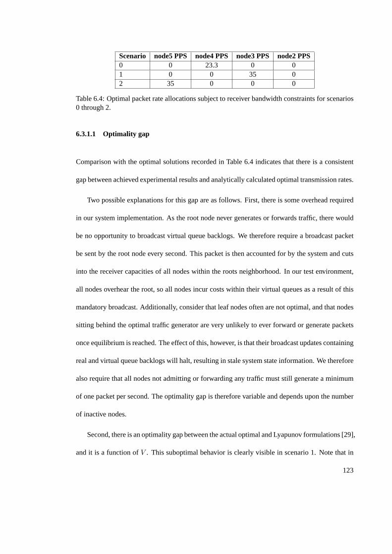
6.5 Achieved packet rate allocations for experimental scenarios 0 through 2. . . . . . 124
6.6 The sum-log utilities achieved for the multi-hop topology using the proportionalfair controller with the PDQ and the MDQ schemes. . . . . . . . . . . . . . . . . 128
and many defense related applications [30]. The motivation and vision behind the use of these
networks is that the low cost, small form factor, devices will allow for a larger number of sensors
to be deployed, increasing the granularity of the sensing information collected. Further, the wire-
less nature of these networks will make deployments easier, and allow for deployments of these
networks in areas where it might not be feasible to have wired infrastructure, e.g., remote isolated
areas where environment monitoring needs to be carried out.
Figure 1.1(a) shows an example of a typical sensor network device, the Tmote Sky [55].
Figure 1.1(b), gives a sense of the form factor of the current devices. Figure 1.1(b) shows that
2
sensor networking devices have already become smaller than the more popular embedded plat-
forms such as cell phones, and the hope is the form factor will be reduced further to the size of
a penny, or may be even smaller. The form factor of these devices imposessevere constraints
on their hardware capabilities. For example, the Tmote Sky platform, which runs the MSP430
microprocessor, which is a 32Khz processor, has 10K RAM and 1MB offlash.
Another important feature of wireless sensor networks, apart from limitedhardware/software
capabilities of the devices, is that these networks are envisioned to have anoperational life span
ranging from a few months to a few years on AA batteries. Thus, given theenergy constraints, the
devices in these networks are fitted with low-power radios. The radios typically follow the IEEE
802.15.4 standard [9], which has become thede-factostandard for wireless sensor network, and
designed to be used with short range devices [9]. The low-power radios, in turn, result in small
packet sizes, typically 40-100 bytes; the goodputs in these networks arein the range of 40-80
bytes/sec for network sizes of 20-40 nodes, with a network diameter of 5-7 hops1. Thus, unlike
IEEE 820.11 [16] based multi-hop wireless networks wireless sensor networks are low-power,
low-rate networks; having severe restrictions on the complexity in terms of thesoftware, and
hence the protocols that can be run over these networks.
A typical routing topology that is found in sensor networks is thecollection tree. Figure 1.2
gives an example of a collection tree2 that might be found in a real sensor network. In Figure 1.2,
node 1 is the sink. All other nodes in this network are sources, that want tosend their sensed
data over the multi-hop collection tree to the sink. The labels on the links represent the success
probability, for a single packet transmission over a wireless link that exists between a given node
1These numbers were obtained from experiments run on the USC Tutornet testbed [46], a 94 node wireless sensornetwork testbed.
2This routing topology was obtained on the USC Tutornet testbed.
3
2
1
0.93
3
0.93
4
0.88
5
0.93
6
8
0.83
0.86
7
0.91
9
0.93
10
0.89
11
12
0.92
0.86
13
14
0.73
0.83
15
0.86
16
0.73
17
0.86
18
0.83
19
0.82
20
0.83
Figure 1.2: A collection tree.
pair. The success probability provides a measure of the quality of the wireless link. During the
course of this thesis, the collection tree will be the recurring routing topologyin our protocol
design and evaluation.
1.2 Capacity region of a network
A key concept necessary for understanding the role of rate control protocols in a packet switched
data network (wired or wireless), is the concept of acapacity region[29] of a network. The ca-
pacity region of a network is defined as the set of rate vectors that are sustainable by the network.
A rate vector is a set of rates, with each element of the rate vector corresponding to a rate allo-
cated to a given source in the network. A rate vector−→r is said to besustainableby the network
if the time average queue size of every router in the network remains bounded when sources in
the network are sending data to their respective destinations at the allocatedrate−→r . A source-
destination pair is referred to as aflow, and hence the capacity region of a network represents the
end-to-end flow rates sustainable by the network. It is important to note thatthe dimensionality
4
Sink
SRC 1 SRC 2
Figure 1.3: A 1-hop topology.
of the capacity region depends on the number of flows that exist in the network. Further, the
boundary of the capacity region is determined by the maximum sustainable flow rates, which in
turn are determined by a combination of protocols implemented at the routing and the MAC layer,
and the link rates presented by the physical layer. The definition of a sustainable rate presented
above is under the assumption that routers in the network have infinite queuesizes, and hence is
useful only from a theoretical perspective. In practical systems, with finite queue sizes, when the
network is operating at a sustainable rate the queue occupancy in the routers will be low, while
at an unsustainable rate the time average value ofcongestedqueues in the network will become
equal to the maximum queue size, resulting in excessive packet drops.
We illustrate the concept of a capacity region by taking the example of a simple one-hop
topology, shown in Figure 1.3, with two sources. For this topology there aretwo sources sending
data to a single destination. The capacity region of this two source network can be represented
by Figure 1.4. The capacity region for this two source network is assumed tobe convex [7].
The region marked feasible represents the set of sustainable rates for this network, and the region
5
0
0.1
0.2
0.3
0.4
0.5
0.6
0.7
0.8
0.9
1
0 0.1 0.2 0.3 0.4 0.5 0.6 0.7 0.8 0.9 1
Src
2 (
Pk
ts/s
ec)
Src 1 (Pkts/sec)
Rate region
Feasible
Infeasible
Figure 1.4: The rate region of the 1-hop topology.
marked infeasible represents the unsustainable rate for this network. Forthis particular example,
since there exist only two sources, the capacity region for the network can be represented by a
two-dimensional plot.
1.3 The need for a rate control protocol
If sources in a network are always operating at a feasible point in the capacity region (Figure 1.4),
the queues in the network will always be bounded, and the network will operate without conges-
tion. In a multi-hop network, however, the sources in the network are unaware of the boundary
of the capacity region, and hence do not have any information about the sustainable flow-rates in
the network. Thus, in a multi-hop network, it is possible that sources start trying to send data to
their destinations at rates that are not sustainable by the network forcing the network to operate
in the infeasible region, resulting incongestion. The goal of the rate control protocol is to try and
avoid/mitigate congestion in the network by performing two key functionalities: first, it detects,
and informs sources, that the network is operating in the infeasible region;second it reduces the
6
flow-rate of sources, bringing the network from an infeasible point of operation to a feasible point
of operation, relieving congestion in the network.
The performance of a rate control protocol is measured in terms of therate-utility presented
to each source in the network. The rate-utility presented to a source is usually given by a concave
function [7] of the rate allocated to the source. If the objective of the rate control protocol is purely
to relieve congestion in the network, the rate control protocol can chooseto operate the network
at any point in the feasible rate region. However, apart from congestion control/avoidance, rate
control protocols are designed toguidethe network to operate at a specific point in the rate region
in order to maximize the sum of the rate-utility of all sources in the network. We willpresent
further details about the different rate-utility functions that the rate control protocol can optimize
for in Chapter 2.
For low-power wireless sensor networks, the degradation of per-source sustainable rate is
quite drastic with increase in network size, because of their limited bandwidths,high density
deployments, and multi-hop-operation. Given the drastic reduction in network capacity with
increase in the size of the network, the motivation for the need for transport layer rate control has
been cited by a few deployed sensor network applications [3, 62]. We can further motivate this
requirement, with the following empirical evidence. In a wireless sensor network testbed [46], it
has been observed that with a 40 byte packet, a 4-node network can give per-source rate as low
as 16 pkts/sec. A 20-node network under similar conditions results in a reduction of per-source
rate to∼ 2 pkts/sec, and in a 40-node network this rate reduces to∼ 0.5 pkts/sec. Thus, even
if low data rate sources are operational in these network (which is typical for a WSN), given the
scarce capacity, a sufficiently large number of such sources can easilycause congestion collapse
7
if they are operating unaware of the sustainable rates in the network. This observation reflects the
importance of rate control protocols in these networks.
1.4 Understanding the need for cross-layer design in wireless networks
Every device capable of communicating over a network has a communication module imple-
mented in software or hardware (or a mix of both) that is referred to as the network stack. The
network stack consists of components that provide functionalities (not necessarily all of them),
such as the transport layer functionality, the routing layer, the MAC and thephysical layer, in
order to allow the device to communicate over the network. The design of network stacks, tar-
geted towards current networking infrastructure for packet switcheddata networks, has primarily
been based on theOpen Systems Interconnection(OSI) model [64]. A good example of a network
stack that is based on the design philosophy of the OSI model is the TCP/IP stack [64]. Under this
model the functionality of the network stack is segregated into different layers; each layer is fully
self-contained, such that in order to perform its functionality a particular layer does not rely on
any other control information, except for the minimalist control information for acknowledging
a packet injected into the underlying layer. The control information for acknowledging a packet
is also binary in nature, only informing the upper layer wether a packet hasbeen received or not,
without explicitly stating the reason for the loss of the packet. To list a few reasons for packet
losses, e.g., packet losses can occur due to network level congestion, MAC level collisions, or bit
errors during transmission at the physical layer.
While the OSI-based architecture of current network stacks (TCP/IP) has served well in the
context of wired networks—in terms of the performance presented by the network stack, as well
8
as the operational flexibility of the stack [31] (this observation is captured by the well known
adage “everything runs over IP, and IP runs over everything”)—thegains presented by this ar-
chitecture diminish significantly when the same network stack is run over multi-hopwireless
networks. This observation is particularly true when considering the specific case of transport
layer rate control for multi-hop wireless networks. The performance degradation of transport
layer rate control in an OSI-based stack such as TCP/IP, over multi-hop wireless networks, is at-
tributed to the minimalist control information exchange between layers of the network stack [2].
In wired networks the binary feedback, in terms of packet acknowledgement control information,
works well since network topology in wired networks are inherently stable,and the underlying
link reliability is exceptionally high; making congestion the primary cause for lossof packets
in wired networks. For wired networks, OSI-based transport layer rate control protocols such
as TCP, thus, interpret the feedback of packet loss correctly as a signal of congestion, and force
sources to cut back their rates performing congestion control functionality efficiently in these net-
works. In wireless networks, however, the frequent change in network structure (due to mobility
or link reliability), and the higher link error rates (as compared to wired networks), makes the
binary packet acknowledgement control information exchange betweenlayers inadequate. In a
wireless network, apart from congestion, a packet could have been lost due to link unreliability,
or due to collisions that might be caused by interference. Thus, due to lackof information, OSI-
based transport layer rate control protocols such as TCP force sources over a wireless network to
woefully underperform, in terms of the flow rates that the sources can achieve [2,18].
Given the failings, due to the OSI-based design, of current network stacks for multi-hop
wireless networks, there has been a shift towards a design philosophy that promotes a more fine
9
grained information exchange between layers. This is referred to as the cross-layer design philos-
ophy. In this approach, the transport, routing, and MAC layer are no longer segregated entities3,
but rely on explicit and fine grained information exchange between the layers to carry out the
functionality assigned to each layer. The cross-layer design philosophyhas strong theoretical
foundations, promoted specifically by the seminal works by Kellyet al. [43], and Low and Lap-
sley [51]. Despite the progress made in developing theoretical frameworks that will enable the
design of cross-layer stacks in multi-hop wireless networks, when considering transport layer rate
control design, to the best of our knowledge, there are no real world implementations that employ
this design philosophy. The aim of this thesis is to design and implement a cross-layer stack with
emphasis on enabling transport layer rate control functionality for a specific type of multi-hop
wireless network, the wireless sensor network. We will now introduce the theoretical founda-
tions that enable a quantitative approach to cross-layer design of transport layer rate control for
wireless sensor network.
1.5 Cross-layer design as an optimization problem
Since the focus of this thesis is on transport layer rate control, we concentrate on presenting
a quantitative description of the approach taken to enable cross-layer design of the rate control
protocol. A key functionality of the rate control protocol at the transportlayer is to inform sources
about the sustainable rate at which they caninject data into the network. The strategy followed
by the rate control protocol for achieving a specific rate allocation is defined by the rate-utility
objective (Section 1.3) the protocol is aiming to optimize. The rate-utility objectives targeted by
3In this thesis we assume the physical layer is a fixed entity, and do not consider cross-layer optimization ap-proaches that also vary parameters at the physical layer, though these have been explored before in the wirelessliterature [36,70,73].
10
the rate control protocol can be to maximize the efficiency of the network, to guarantee a fair rate
allocation to all sources in the network, or to provide a balance between efficiency and fairness
in terms of allocated rates. As mentioned in Section 1.3, the rate-utility for a source i is usually a
concave function of the allocated rateri given bygi(ri). The exact form of the functiongi(ri) is
determined by the objective that the rate control protocol is striving to achieve. The cross-layer
design of the transport layer rate control can then be posed as a constrained optimization problem
in the following form:
P : max∑
ri∈−→r
gi(ri)
s.t −→r ∈ Λ
HereΛ is the capacity region of the network. If the objective in the above optimization prob-
lem is concave, and the capacity regionΛ is convex, then the optimization problem is convex [7]
and we can find a unique rate vector−→r , within the capacity region, that can maximize the global
objective function∑
ri∈−→r
gi(ri).
If for a given network we are able to formulate the rate control problem in the above form, we
can use a centralized convex programming solver to obtain solutions to this problem, thus per-
forming rate control in a centralized manner. However, in general, since centralized solutions are
not flexible to network dynamics (such as mobility, flow dynamics, node failures, link failures,
etc.), and do not scale well with the size of the network4 [15], we focus on designing rate control
algorithms that can achieve a solution to the above optimization problem in a distributed manner.
4While it’s a broadly accepted notion that decentralized protocol design is a more efficient design principle, thereare instances when centralized design principles have been promoted. Examples are solutions to the coverage problemin wireless sensor networks [52], enterprise management of campuswide networks [10], and even in rate control forheterogeneous wireless sensor networks [63,71].
11
Distributed algorithms have the ability to make local decisions based on neighborhood infor-
mation, such that these local decisions will result in a global optimum, making the algorithms
adaptable to network dynamics, and scalable with the size of the network.
From a theoretical perspective, the seminal works by Kellyet al. [43], and Low and Laps-
ley [51], highlighted the power of using duality-based techniques in findingcross-layer distributed
solutions to the problemP, at least in a wired setting. These ideas were then used to formulate
theoretical proposals for such solutions in a wireless setting as well ( [13], [95]). More recently,
the works by Stolyar [83] and Neelyet al. [58] have built upon these seminal contributions, and
have shown that elegant, and modular distributed solutions to the problemP can be designed by
appropriately modifying the MAC layer, and allowing sources to make rate allocation decisions
purely based on the occupancy of their local queues. Despite the advances made in theoretical
understanding of the problemP, it is only recently that attempts are being made to convert these
theoretical contributions into real world protocols, especially in the contextof multi-hop wireless
networks.
1.6 Understanding requirements for transport layer rate control in
WSN
Given the need for congestion control, there have been numerous proposals ( [93], [67], [63],
[101], [71]) that can perform congestion control in these networks.However, apart from the
core functionality of congestion control, we believe rate control protocolstargeted towards a
WSN should exhibit two important characteristics. First, they should beresponsive, exhibiting
the ability to inform sources about the sustainable rates in as small a duration as possible. The
12
need for rate control protocols to be responsive is primarily due to energy efficiency concerns.
Since in these networks, apart from bandwidth, energy is also a scarceresource, and radios are
considered to be the primary consumers of energy, it is imperative to reduce the active duration
of these radios. This can be achieved by ensuring short flow completion times, since short flows
directly imply shorter uptime for the radios. If the rate control protocols are responsive, they will
be able to inform sources about the sustainable rates in a shorter duration, allowing the sources
to transmit at a faster rate in a much shorter time frame leading to shorter flow completion times.
Second, rate control protocols for WSN should have theflexibility to optimize for different types
of rate-utility functions. This characteristic is important, particularly in a sensor network setting,
due to the diverse nature of the applications envisioned to be operated over these networks. Thus,
rate control protocols in WSN should not be designed to optimize for a single utility function,
rather the rate control stack should be flexible enough, having the ability to optimize for any
utility function presented by the application.
State of the art designs for rate control protocol in wireless sensor networks are however
primarily heuristics, that rely on additive increase multiplicative decrease (AIMD) mechanisms.
They suffer from long convergence times and large end-to-end packet delays. In addition to be-
ing based on heuristics, state of the art rate control protocols for wireless sensor networks are
monolithic in design. The monolithic protocol design caters for optimizing a specific utility func-
tion (such as max-min fairness), or performing purely congestion controlfunctionality without
regard for optimization. Thus, although state of the art rate control protocols for WSN perform
the core task of congestion control, they are deficient in terms of the abovementioned desired
characteristics for such protocols in a WSN context.
13
1.7 Contributions
The contributions of this thesis are two rate control protocols that aim to address the deficien-
cies of state of the art for rate control in WSN, as discussed in Section 1.6.The novelty in both
the protocols is the quantitative approach we have pursued in our design,allowing us to realize
the powerful theoretical frameworks proposed for achieving a distributed solution to the prob-
lemP (Section 1.5) in practice. The first, called theWireless Rate Control Protocol (WRCP),
addresses the issue of convergence times and end-to-end packet delay using explicit capacity in-
formation. The Wireless Rate Control Protocol presents a distributed solution to the lexicographic
max-min fairness problem over a collection tree. It uses a novel interference model, called the
receiver capacity model, in order to define the capacity region of a wireless sensor network em-
ploying a Carrier Sense Medium Access with Collision Avoidance (CSMA-CA) MAC. The use
of this model allows WRCP to achieve fast convergence time and small end-to-end packet delays.
The second, called theBackpressure-based Rate Control protocol (BRCP), presents aflexible
rate control protocol that can optimize for any global concave objectivefunction using purely
local queue information. The backpressure-based rate control protocol presents a more generic
solution to the problemP. It has been designed using stochastic optimization techniques that
allow it to optimize for any concave utility function (g(ri)) by simply using local queue informa-
tion. The generic solution provides different, rate-utility specific, transport layer,flow controllers
to work with this protocol. Each flow controller aims to optimize a specific application-defined
concave rate-utility function. These different flow controllers can be presented to the applica-
tion developer as a set of libraries, allowing the user the flexibility to pick and choose the flow
controller, to be used with BRCP, that will aim to optimize his application specific rate-utility
14
function. Both, WRCP and BRCP, highlight the gains that can be achieved by pursuing a more
theoretical approach to rate control design for wireless networks in general, and wireless sensor
networks specifically.
1.8 Organization
The organization of this thesis is as follows: InChapter 2we proceed to explain quantitatively
the different objectives that a rate control protocol can strive to achieve. In Chapter 3, in order
to put the contributions of thesis into perspective, we present prior art pertaining to rate control
design in wired and wireless networks. InChapter 4we present a novel interference model
called the receiver capacity model that will allow us to define the constraints of the problem
P(Section 1.5), and hence will form the crux of the analytical framework onwhich the protocols
proposed in chapters 5 and 6 are based. InChapter 5we present theWireless Rate Control
Protocol (WRCP) protocol, an explicit and precise rate control protocol, that hasthe ability to
achieve a lexicographic max-min fair rate allocation over a WSN collection tree.In Chapter 6we
present the design and implementation of theBackpressure-based Rate Control Protocol(BRCP).
BRCP relies on a collection offlow controllersthat can be presented to the user as a library, each
flow controller having been designed to optimize for an application specific concave rate-utility
function. In Chapter 7, we present a rigorous empirical evaluation of this backpressure-based
protocol (BRCP), to understand the various design choices that can bemade, in terms of the
algorithms and parameters, while implementing the MAC and Transport layers ofthis stack in a
WSN setting. Finally, inChapter 8, we present a summary of the contributions of this work, as
15
well as a discussion to highlight the various open problems associated with thiswork and which
can form the foundation of future research based on this thesis.
16
Chapter 2
Defining Objectives for a Rate Control Protocol
In Chapter 1, we showed that a cross-layer design of a transport layer rate control protocol can be
undertaken, by formulating the problem in the following form:
P1 : max∑
ri∈−→r
gi(ri)
s.t −→r ∈ Λ
Assuming that the constraints are well defined (in Chapter 4, we show how we quantify these
constraints for a wireless sensor network), in order to use the formulationP1 to design rate
control protocols for a network, we need to define the objective functiongi(ri).
In general the rate-utility functiongi(ri) can be any concave function. Thus, there is an
infinity of objectives that can be defined for rate control protocols. However, in this thesis we
shall focus on three specific objectives. We aim to design a rate control protocol that can either
try to maximizenetwork utilization, or it can try to optimize forfairness, or it can try to find a
good trade-off betweennetwork utilization1 and fairness, by trying to maximize utilization while
achieving a certain level of fairness. We focus our efforts on these three objectives, since it
1We will be using the termsnetwork utilizationandnetwork utilizationinterchangeably.
17
has been shown that, in general, the objectives of maximizing network utilizationand achieving
fairness are diametrically opposite [66,88], and hence represent the two extremes of the spectrum
of possible objectives. The third objective, of achieving a balance between maximizing utilization
and fairness, finds a middle ground between these two extremes. Thus, webelieve these three
objectives are a good sample, from the entire spectrum of objectives, to showcase the cross-layer
design of transport layer rate control protocols that aim to solve the problemP1.
We now discuss the three objective functions that a rate control protocolcan use in order to
maximize network utilization, to optimize fairness, or to achieve a good balance between fairness
and utilization.
2.1 Maximizing network utilization
In order to maximize for network utilization the rate control problem can defined as:
P2 : max∑
ri∈−→r
ri
s.t −→r ∈ Λ
As mentioned earlier, maximizing network utilization requires the maximization of sum rate.
In wireless networks solutions for the above optimization problem would generally involve allo-
cating all the rate to one or more of the first hop nodes. As is evident, such asolution is inherently
unfair (since any node farther then a single hop will not be able to communicate), making solu-
tions to this problem quite useless in practice.
18
2.2 Lexicographic max-min fairness
A lexicographic max-min fair rate vector−→r∗ is a rate vector, such that if the elements of the max-
min fair rate vector−→r∗ are arranged in ascending order, for any othersustainablerate vector
−→r
whose elements are also arranged in ascending order,−→r∗ will always be lexicographically greater
than−→r , i.e. there exists aj, such thatr∗j > rj , and∀ i, 0 < i < j, r∗i = ri.
The physical interpretation of the above definition, for lexicographic max-min fairness, can
be better understood by taking the example of max-min fairness in wired networks. In the case of
wired networks, a necessary and sufficient condition for a lexicographic max-min fair rate vector
is the following: a rate vector is said to be max-min fair, if and only if every flow inthe network
has at least one bottlenecked link. A flow is said to be bottlenecked at a link, ifthe flow has the
highest rate amongst all flows sharing this link and the capacity of the link hasbeen exhausted.
A proof for the necessary and sufficient condition, for a wired network, can be found in [4].
An intuitive understanding of lexicographic max-min fairness can be obtained by the following
example: imagine a wired network where each node in the wired network is replaced by a vessel
of certain capacity, and the links are replaced by pipes. If sources were to pump water into these
pipes from the leaves of this network, each of the flows can keep increasing its rate till they hit
a vessel whose capacity has been exceeded. The first such vesselfor a given flow is called the
bottleneck link for that flow. All flows that have the same bottleneck link will share the same rate.
19
Max-min fairness can be quantified as an optimization problem by using the notion of α-
fairness, .α-fairness is defined as follows:
P3 : max∑
ri∈−→r
r1−αi
1−α
s.t −→r ∈ Λ
As α → ∞, it can be shown that the solution to the above optimization problem satisfies the
necessary and sufficient condition of a lexicographic max-min fair vector. In Chapter 6, we show
that in practice, for sensor networks, the solutions forα-fairness starts approaching the max-min
fair solution even forα values as small as5.
2.3 Proportional fairness
A well known utility function that is able to achieve agood trade-off between fairness and uti-
lization is the log rate-utility function [66]. This is also known as proportional fairness. A rate
control problem solving for proportional fairness is defined as follows:
P4 : max∑
ri∈−→r
log(ri)
s.t −→r ∈ Λ
Note that since the objective function is a sum of logarithms, maximizing the objective func-
tion implies maximizing the product of the rates (∏
ri∈−→r
(ri)). In order to maximize the product of
rates, the solution has to ensure that there is no source who is starved (given a zero rate). Also,
sources that create more congestion, or result in larger backlogs, should be given a smaller rate.
Intuitively, sources that have a larger hop count to the destination will require to traverse more
20
links resulting in consumption of larger amounts of capacity (resulting in higheramounts of con-
gestion), as compared to sources that are closer to the destination. Proportional fairness thus tries
to be partial to sources that are closer to the destination, while ensuring thatthere is no source that
is starved. Proportionally fair solutions thus try to satisfy the inherent tension that exist between
the problems of maximizing network utilization and optimizing fairness [66].
2.4 Summary
In this chapter we quantified the objective∑
ri∈−→r
gi(ri) that rate control protocols developed in this
thesis will strive to optimize. While there are an infinity of objectives that rate control protocols
can be designed to optimize, in this thesis we focus on three specific objectives: maximizing
network utilization, max-min fairness and proportional fairness. We focuson these three objec-
tives since the objective of maximizing network utilization and max-min fairness represent two
extremes, of the spectrum of objectives that a rate control protocol cantry to optimize, while
proportional fairness represents agood trade-off between maximizing network utilization and
max-min fairness. We therefore believe that the three objectives are a good sample of the entire
spectrum of objectives.
As will be seen in the following chapters, using theoretical frameworks thatsolve for the
generic rate control problemP1 result in elegant design of rate control protocols. Despite the
elegant design, and the strong theoretical foundations for these designs, that result from for-
mulating the rate control problem as a constrained optimization problemP1, it is important to
understand the limitations of this mathematical formulation. A key limitation of the problemP1
is that the optimal allocated rater∗i , that will maximize the global concave rate-utility function
21
∑
ri∈−→r
gi(ri), is a long-term time-average rate. This implies that this formulation is relevant only
for long flows. It is unclear what this formulation says about short flows. Another limitation of
this formulation is that it does not represent the class of problems, where rate control protocols
need to be optimized for delay instead of throughput. In order to solve the problemP1 optimally,
the optimal rate vector−→r ∗ will make the constraints of the problemP1 tight. This implies that
the optimal rate vector, that will solve for the problemP1, will lie on the boundary of the rate
region. Operating at this optimal rate vector will therefore involve larger queue sizes, than operat-
ing at a sub-optimal rate vector within the rate region. This inherent tension between optimizing
rate-based utility function and delay, is the reason whyP1 cannot be used to represent the class
of rate control problems that want to optimize for delay.
22
Chapter 3
State of the Art
3.1 Congestion control in wired networks
The seminal work by Jacobson [35] was one of the first congestion avoidance mechanisms built
into the Internet. The work by Jacobson [35] introduced several algorithms, such as the slow-
start mechanism, and theAdditive Increase Multiplicative Decrease(AIMD) algorithm that form
the core of today’s Transmission Control Protocol (TCP) [64]. The version of TCP that first
incorporated the algorithms proposed by Jacobson [35], is known as TCP Tahoe and made its
appearance in the Internet as part of the BSD 4.3 operating system’s network stack [8]. The slow-
start and AIMD mechanism, that are core to the congestion avoidance algorithm in TCP, perform
end-to-end congestion control by using loss of packet acknowledgements as a sign of congestion
in the network. These algorithms allow TCP to treat the network as ablack box, giving it the
ability to perform congestion control irrespective of the type of network.
TCP Tahoe was considered to be too conservative in its multiplicative decrease mechanism,
forcing slow start whenever a packet is lost (even after the packet is successfully retransmitted),
23
thus reacting over-aggressively to transient congestion and hurting TCP throughput. The sub-
sequent versions of TCP Tahoe, such as Reno and SACK [22], improve upon the performance
of TCP Tahoe by introducing mechanisms that allow it to detect the transient congestion in the
network better; avoiding over-throttling of TCP throughput when intermittentpacket losses oc-
cur due to transient congestion. Another version of TCP, called TCP Vegas [8], was developed
to improve significantly on the throughput performance of TCP Reno. TCP Vegas achieves this
improvement by introducing a new congestion avoidance scheme. TCP Vegas improves the con-
gestion avoidance mechanism by introducing a new bandwidth estimation schemethat looks at
the actual throughput and estimated throughput of TCP to regulate its congestion window size,
in order to better estimate the available bandwidth and avoid congestion. The key idea behind
TCP Vegas is that in a congestion free network the difference between theactual and estimated
throughput will be negligible, while in a congested network the difference quantifies the amount
of congestion in the network, and the congestion window should be reduced by this amount.
Compared to the fine grained bandwidth estimation of TCP Vegas, the multiplicativedecrease
mechanism used by TCP Reno to avoid congestion is too aggressive — it cutsits rate by half
whenever its sees packet losses — resulting in TCP Vegas outperforming TCP Reno in terms of
achieved throughput.
While the end-to-end congestion control mechanism of TCP made it network agnostic —
allowing applications to run over networks, irrespective of the type of the network — it also pre-
sented some severe drawbacks. In high-speed connections with large delay-bandwidth products,
the end-to-end congestion mechanism of TCP resulted in large queues, and hence high delays;
since, in the absence of explicit feedback from the network TCP relies solely on packet drops
for detecting congestion, resulting in queues growing to large values whenTCP operates at high
24
throughput. Further, TCP introduced periodicity into the traffic, forcing global synchronization of
the additive increase multiplicative decrease phases of traffic, leading to severe underutilization
of the network. To counter these drawbacks, resulting in large delays and global synchronization
of traffic, Active Queue Management (AQM) techniques were proposed. In AQM, the interme-
diate routers take part in congestion avoidance, by observing their queue sizes and proactively
marking packets withcongestion bits, or by proactively dropping packets to send congestion
signal back to the end hosts. By introducing randomness into the marking/dropping of packets
AQM techniques were able to reduce forwarding queue sizes and avoid the global synchroniza-
tion problems introduced by the end-to-end congestion control mechanism of TCP. One of the
first AQM mechanisms was theRandom Early Detection(RED) algorithm proposed by Flloydet
al. [25]. The key problem with AQM techniques such as RED and SRED [91],is that their perfor-
mance is extremely sensitive to parameter settings. Subsequently proposed algorithms, such as
BLUE [24], AVQ [45] and PI [33], present a more control-theoretic design of AQM mechanisms
whose parameters can be estimated on the fly (based on traffic load, and traffic pattern).
An alternative to AQM, for improving the performance of end-to-end congestion control
mechanism of TCP in large delay-bandwidth products was proposed in the form of FAST TCP [98].
FAST TCP is a variant of TCP, employing end-to-end congestion control, where the window
control mechanism is based on a delay-based estimation technique, rather than a loss-based es-
timation technique as is the case with the existing implementations of TCP. The window control
algorithm uses an estimate of the queueing delay experienced by the packets, to determine the
number of packets that are buffered in the network; the amount by which the window is in-
cremented or decremented depends on how many buffered packets existin the network when
25
compared to a targeted buffer value. The design of FAST TCP is pursuedin [98] by Jinet al., us-
ing a constrained optimization-based [7] framework. The quantitative approach taken by Jinet al.
allows the authors to prove the stability and proportional fairness of the delay-based estimation
technique for congestion control, used in FAST TCP, when operating in high delay-bandwidth
product networks.
In the recent past there have been proposals promoting a paradigm shift in the philosophy be-
hind congestion control in the internet; promoting the idea of moving away fromend-to-end con-
gestion, treating the network as a black box, and making congestion controlmore router-centric.
In the Internet context, recent protocols such as XCP [41] and RCP [19] have highlighted the
gains of using precise feedback using network capacity information, as compared to traditional
AIMD approaches followed by TCP and its many variants. XCP [41] is a window based protocol
that presents improved stability in high delay bandwidth networks, and RCP is arate based pro-
tocol that improves the flow completion times for short flows. The idea of usingrouter-centric
explicit/precise feedback regarding available capacity to perform congestion control is not spe-
cific to the internet, and there exist proposals in the ATM network literature where mechanisms
have been proposed for providing explicit and precise congestion feedback using the resource
management (RM) cells for ABR (available bit rate) traffic ( [6], [61], [40] and [82]).
3.2 Congestion control in 802.11-based multi-hop wireless networks
The creation of the IEEE 802.11 standards [16] for aCarrier Sense Medium Access with Collision
Avoidance(CSMA-CA) protocol, for single and multi-hop packet switched wireless networks,
spawned research in the domain of multi-hop wireless packet switched networks. The success of
26
TCP, as a transport layer, in the wired Internet led researchers to experiment with the TCP/IP stack
over 802.11-based wireless networks. This lead to the realization of the inadequacy of the con-
gestion detection mechanism of TCP, leading to excessive false detection ofcongestion, resulting
in the heavy underutilization of the network capacity [2,18], or an unfair allocation of bandwidth
to contending flows [68]. The shortcomings of TCP over wireless networks was primarily due
to the assumption that a packet loss is a sufficient and necessary conditionfor congestion in the
network. While packet loss is good indicator of congestion in wired networks [35], in wireless
networks packet losses could occur due to buffer overflows (congestion), link errors, frequent
route changes due to mobility, or collision due to interference [2, 18]. Thus, using packet loss as
a sufficientsignal of congestion can force TCP to woefully underperform in a wireless network.
Further, in wired networks a source can cause congestion only in router/nodes through which it’s
routing its traffic; in wireless networks, however, the broadcast natureof the wireless medium
allows sources to cause congestion even at nodes that are not routing their traffic. Thus, in a
wireless network a flow might not incur packet loss and still might be responsible for causing
congestion. Therefore treating packet losses as a necessary condition for congestion is incorrect.
The failure of the congestion detection mechanism in TCP, over wireless links, prompted
researchers to explore new techniques for congestion detection/avoidance strategies that will im-
prove upon the performance of TCP over wireless. One set of proposals (TCP-F [11], TCP-
ELFN [32], TCP-BuS [44], ATCP [50], EPLN/BEAD [105]) that aimed at solving transport layer
rate/congestion control in a multi-hop wireless setting, focused on improving the performance of
TCP over wireless. They strove to achieve this objective by introducing mechanisms to better
inform TCP of the exact reason for packet loss over a wireless link. Bypresenting the exact rea-
son for packet loss to TCP, they could freeze the flow-control window in TCP when congestion
27
was not the cause of packet loss, and allow TCP’s default congestion avoidance mechanism to
function when packet loss occurred due to buffer overflows.
While these proposals helped in solving the problem of treating packet loss as asufficient
signal of congestion, and improved network utilization, they still did not address the issue of
unfairness introduced by treating packet loss as anecessarycondition for congestion. To rectify
the second problem, researchers have undertaken a neighborhood-centric view of congestion [67,
68], as compared to a host-centric view of congestion. By assuming packetloss (due to buffer
overflows) as a necessary condition for a signal of congestion, TCP assumes a host-centric view,
assuming that a source can cause congestion only in nodes/routers that are forwarding its data.
In a neighborhood-centric view, congestion at a specific node/router iscaused not only by the
sources whose data the specific node is routing, but also by sources whose traffic is being routed
by nodes within the neighborhood of the congested node. Link-RED [27]and NRED [103]
are active queue management policies, similar to RED [25], that are implicitly (Link-RED) or
explicitly (NRED) based on the design of the neighborhood-centric view ofcongestion.
Given the need for a neighborhood-centric view of congestion, and the failings of TCP in
wireless, there has also been a significant push forclean slatedesign of congestion/rate control
mechanisms over wireless networks, independent of TCP. Examples are ATP [84], EWCCP [87],
WCP [68] and WCPCAP [68]. Of these, EWCCP, WCP and WCPCAP explicitlydesign con-
gestion detection and rate allocation mechanisms that take the neighborhood-centric view into
account. EWCCP is based on a cross-layer design principal, similar to the protocols proposed in
this thesis, and aims to achieve proportional fairness amongst flows in a wireless ad-hoc network.
EWCCP has however never been implemented in a real system. WCP [68] uses an AIMD mech-
anism to present a clean slate design of a transport protocol for wireless ad-hoc network. The
28
protocol is router-centric, and explicitly shares congestion amongst all neighbors of a congested
node by asking all sources whose data is being routed through the congested nodes neighbor-
hood to perform multiplicative decrease on their rates, on detecting congestion. By sharing the
congestion signal equally amongst the nodes of a neighborhood it aims to achieve lexicographic
max-min fair rate allocation amongst the flows. WCPCAP [68] is an explicit and precise rate
control protocol designed for wireless ad-hoc networks. It uses themodel proposed in [38] to
calculate the exact available capacity in an 802.11-based wireless ad-hocnetwork, and shares
this capacity equally amongst contending flows in order to achieve a lexicographic max-min fair
rate.
3.3 Congestion control in wireless sensor networks
In the recent pastWireless Sensor Networks(WSN) emerged as a sub-domain of the research per-
formed on multi-hop wireless networks. WSN share quite a bit of similarity with 802.11-based
multi-hop wireless networks, in terms of the network structures and network dynamics; due the
use of a wireless medium as the physical layer, and the use ofCarrier Sense Meidum Access
as the de-facto MAC protocol in both type of networks. WSN are multi-hop wireless networks,
composed of low rate, low powered, embedded devices having sensing capabilities. These net-
works are targeted towards sensing applications such as structural health monitoring [62], habitat
monitoring [85], sensing seismic activity [99], etc. The need for congestion control has been
demonstrated in wireless sensor networks [63, 67]. Given the importanceof this problem, there
have been a series of proposals aiming to mitigate the affects of congestion in aWSN. We sum-
marize some of the key papers: ARC [101] proposes an AIMD rate control strategy whereby the
29
nodes increase rates proportional to the size of their sub tree and performs multiplicative decrease
on sensing packet drops. ESRT [71] is a sink-centric approach that measures available capacity
and allows for rate increments and decrements by observing the ability of sources achieve a
certain event detection reliability target. CODA [93], provides for both open-loop hop-by-hop
back-pressure and closed-loop multi-source regulation whereby sources vary their rate based on
feedback from the sink. FUSION [34] uses a token based regulation scheme that allows for addi-
tive increase of source rates. It detects congestion using queue lengths and mitigates congestion
by a combination of hop by hop back pressure and an adaptive MAC backoff scheme. In the
work by Ee and Bajcsy [20], each node determines its own average aggregate outgoing rate as
the inverse of its service time for packets and shares this rate equally amongst the nodes served
in the subtree. This scheme does not always achieve a max-min fair solution as information is
not shared explicitly with neighbors. IFRC [67] is a state of the art distributed approach that
mitigates congestion by sharing congestion information explicitly with the set of allpotential in-
terferes of a node, and uses AIMD to react to the feedback. However, its design focuses primarily
on achieving steady state fairness rather than rapid convergence or lowdelay. RCRT [63] is a
recent centralized scheme where the sink employs an AIMD mechanism to calculate achievable
rates and explicitly informs the sources as to the rate as which they can transmit.A common
theme in most of these proposals is to use an AIMD mechanism to set rates, because they are ag-
nostic to the underlying MAC and therefore lack fine-grained information regarding achievable
network capacity.
30
3.4 Using cross layer optimization for rate control design
As can be seen from the progression of research in congestion control in wired and wireless
networks, there has been a growing awareness that transport layer rate control functionality can
be greatly improved by increasing the information exchange across layers(Transport, Routing
and MAC). Further, there has also been a realization that transport layer rate control has primarily
been an undertaking using heuristics. This has led to the pursuit of a more theoretically rigorous
framework for quantifying the problem of transport layer rate control (e.g. FAST TCP [98]),
and developing techniques that will result in algorithms which can achieve a cross-layer design.
While, in the wired Internet, rate control protocols developed using cross-layer design principles
(such as XCP [41] and RCP [19]) have faced tempered skepticism — dueto the incumbent nature
of TCP in these networks, and the modifications required to intermediate routers — the adoption
of these design principles for wireless networks has been more forthcoming. We proceed to
highlight some of the work in this area, that have been responsible in developing and promoting
the cross-layer design philosophy.
The 1998 paper by Kellyet al. [43] was a seminal one in the area of analysis of rate control
in networks. It established that distributed additive increase-multiplicative decrease rate control
protocols can be derived as solutions to an appropriately formulated optimization problem. The
solutions can be interpreted as rate adaptation in response to shadow prices. This was followed by
a classic work by Low and Lapsley [51] in which the Lagrange dual of theoptimization problem
is derived and a sub-gradient approach is used to solve the optimization problem in a distributed
manner. Since then, there has been a substantial literature, primarily in the wired context, that
has focused on understanding not only rate control but other networkprotocols across multiple
31
layers in the context of optimization problems that they seek to solve. This has led to the unifying
view that layered and cross-layer protocol design can be understoodfundamentally as the result
of an appropriate decomposition of a network utility maximization problem. An elegant survey
conveying this view of the literature is the recent article by Chianget al. [14].
Given its compelling nature and power, it is hardly surprising that optimization approaches
have been used for analysis and design of wireless network protocols as well. On the design
side there have been a number of papers on cross-layer optimization in wireless networks: Of
particular note are the authoritative papers by Chiang [13] and Johansson et al. [39], as well
the works by Wang and Kar [95], Yuanet al. [106], Liu et al. [49], Mo et al. [53]. Many of
these works focus on joint Transport and PHY/MAC optimization, and propose sub-gradient
algorithms based on the primal as well as the Lagrange dual. In our own previous work in this
direction [75], [76], we have focused on the particular problem of fairand efficient data-gathering
on a tree and developed a Lagrange dual-based sub-gradient algorithm for it.
The past couple of years have also seen the emergence of new approaches that consider
time-varying channels and provide for stochastic optimization. This approach is described by
Neely [57], and expanded on in the monograph by Georgiadis [29]; another related work is by Xi
and Yeh [102]. Approaches similar to the one proposed by Neely [57], have been proposed by
Stolyar [83], Eryilmaz [21] and Lee [47]. These distributed approaches use neighborhood queue
backlog occupancy information to make online transmission decisions. Connections between
this stochastic optimization approach and the static optimization approaches are still being dis-
covered, but it is already clear that these stochastic approaches are particularly useful for wireless
networks showing a high level of link dynamics.
32
3.5 Backpressure-based rate control mechanisms
Recently, there been an increasing effort to convert the theoretical frameworks proposed by
Neely [57] and Stolyar [83], for solving the stochastic optimization problem of transport layer
flow control using backpressure-based algorithms, into real world network stacks. Most notable
are the works by Warrieret al. [96], Akyol et al. [1] and Radunovicet al. [65]. The work by
Warrieret al. [96] shows a practical mechanism of implementing backpressure-based,differen-
tial queue scheduling, in existing CSMA based protocols. They however do not present any
insights to the design of flow controllers that need to sit on top of their modified CSMA MAC
for optimizing some global utility function. The work by Akyolet al. [1], apart from present-
ing a practical backpressure-based scheduling scheme on existing CSMA MAC’s, similar to the
work by Warrieret al. [96], also aim at building a flexible congestion control algorithm that can
optimize any concave global utility function. The work by Akyolet al. [1] uses a primal/dual
based greedy algorithm to solve the general optimization problemP presented in chapter 1. The
greedy algorithm emulates a gradient based search and results in an additive increase style algo-
rithm where the exponential time average rate is incremented based on the queue backlogs. The
work by Radunovicet al. [65] develops a multipath routing and rate control protocol, that can
be integrated with TCP over 802.11, using backpressure-based techniques. They use a simple
backpressure scheduler that allows transmissions as long as the queue differential is greater than
a threshold.
33
3.6 Capacity models for wireless networks
As shown in chapters 1 and 2, the main challenge in quantifying the transportlayer rate control
problem, as a constrained optimization problem, is to have a model that presents constraints
which characterize the capacity region of the network [29]. A good survey of the models used in
wireless networking research is presented in [53]. Among the most commonlyused models are
graph-based models, such as the clique capacity model ( [12], [17]). The clique capacity model
characterizes the capacity region of the network by presenting constraints associated with each
clique existing in the network.
Researcher have also used link-based models, such as the slotted ALOHAmodel [94]. This
model captures the link capacity between each sender-receiver pair asa success probability of a
packet transmission on that link. The success probability on the link is calculated as the prob-
ability that the link is active, given that no other link between in the given neighborhood of the
receiver is active. The constraints generated by the ALOHA model is simplythat the rate allo-
cated to each link should be less than the success probability on that link. Thekey drawback of
this model is that it is very specific to the slotted ALOHA protocol. Apart from the graph-based
and link-based models, researchers have also used aSignal to Noise Interference Ratio(SNIR)
model [13]. In the SNIR model the link capacity is defined as the shannon capacity. In order to
characterize the rate region of the network the model then sets a constrainton each link of the
network, such that the link transmission rate should be less than the shannoncapacity of the link.
Apart from the generic models described here, more recently there has been an effort to build
accurate 802.11 CSMA MAC [16] specific models, to characterize the capacity region of an
802.11-based multi-hop network. These models are similar to the ALOHA model, inthat they
34
aim at calculating the link capacity of each link in the network, similar to the ALOHA model. The
capacity of a link is equated to the success probability of a transmission between a sender-receiver
pair. The calculation of the success probability is done by performing a markovian analysis on
a state space transition diagram of an 802.11-based multi-hop network. Thework by Jindalet
al. [38] is the most result in this effort.
3.7 Positioning of our contributions
The Wireless Rate Control Protocol(WRCP), presented in Chapter 5, is similar in spirit to
RCP [19] in its design and goals, since it is a rate-based protocol and attempts to shorten the
flow completion times by explicitly allocating rates based on available capacity in the network.
In an 802.11 multi-hop wireless setting, WCPCAP [68] is similar in nature to WRCP.WCPCAP
is a distributed rate control protocol that can achieve max-min fairness using explicit capacity
information. The key difference between WCPCAP and WRCP is that WCPCAP relies on a
model [38] that is very specific to an 802.11 multi-hop network. It is not clear how this model
can be ported to a sensor network setting. WRCP on the other uses a very simple model, that we
show works well in the context of a CSMA MAC for sensor networks. Further, WCPCAP does
not cater for external interference, or present validation for its parameter settings, whereas as we
will demonstrate, WRCP works well in the presence of external interference, and the parameter
settings for WRCP are better understood.
The Backpressure-based Rate Control Protocolpresented in chapters 6 and 7 is our con-
tribution to convert the theoretical frameworks, resulting in backpressure-based algorithms for
solving stochastic optimization problem of transport layer rate control, into real world protocols.
35
In Chapter 6, we use the theoretical framework presented by Neelyet al. [58] to design aflexible
rate control protocol that can optimize foranyapplication specific concave rate-utility function.
Akyol et al. [1] presented a similar proposal to our work presented in Chapter 6 in the same time
frame. The key difference between their work and our proposal (BRCP), is the stochastic opti-
mization technique used in designing the congestion control algorithm, which are complimentary
to each other making the congestion control algorithms complementary to each other as well.
The technique used by us relies on the Lyapunov drift framework presented by Neely [58]. This
technique is complementary to the primal dual technique used in [1] and presents a purely queue-
ing theoretic approach to solve the optimization problemP. Our proposal thus relies on setting
instantaneous rates based on the queue backlog at a node, instead of using time averages and
additive increase mechanisms used by Akyolet al.[1]. In Chapter 7 we add to this effort, of mak-
ing backpressure-based protocols a reality, by undertaking a thorough empirical evaluation of the
various design choices available to achieve an efficient implementation of a backpressure-based
protocol. In Chapter 7, we show that in order to achieve the gains envisioned by implementing a
backpressure-based protocol, at least in a sensor network setting, we do not need to implement the
complicated heuristics presented by Warrieret al. [96] and Akyolet al. [1]. Instead we can have
a naive scheduler that allows the network layer to inject packets into the MAClayer as long as
the node has a positive queue differential with its parent, and achieve the same gains as claimed
by Warrieret al. and Akyol et al.. In Chapter 7, we also show the parametric dependence of
the backpressure-based stack, and motivate the argument for automatic parameter adaptation in
order to ensure the performance gains promised by the backpressure-based designs. The empir-
ical evaluation presented in Chapter 7 is the first of its kind, and raises someopen problems not
highlighted in previous proposals ( [65], [1], [96]).
36
Our design of WRCP and BRCP has been enabled by the use of thereceiver capacity model
(Chapter 4). It quantifies the capacity presented by a receiver to flowsthat are incident on the
receiver, and presents constraints local to the receiver, that defines the bandwidth sharing that
takes place between flows incident on a receiver. The model is particularly useful in our setting,
since it caters to a CSMA based wireless sensor network. There are other interference models in
the literature. Among the most commonly used models are graph based models, such as the clique
capacity model ( [12], [17]), and link based models such as the SINR model [13] and the ALOHA
model [94]. We believe these models, which have been largely used in theoretical studies, are not
well suited to CSMA-based networks. The clique capacity model does not present purely local
constraints, making it hard to realize distributed algorithms using this model; the SINR model is
more akin to modeling MAC’s with variable bit rate radios; the ALOHA model is very specific to
the ALOHA MAC. The model presented by Jindalet al. [38] captures the capacity region of an
802.11 multi-hop wireless network quite accurately, however it is not clear how this model can
be ported to be used in a wireless sensor network setting.
37
Chapter 4
Receiver Capacity Model1
In Chapter 1, we showed that the problem of rate control can be written asa constrained opti-
mization problem as follows:
P : max∑
ri∈−→r
gi(ri)
s.t −→r ∈ Λ
For a given concave utility functiongi(ri), the key challenge in quantifying the problemP1
is to estimate the constraints of this optimization problem. The constraints of the problemP1 are,
in turn, defined by the capacity regionΛ of the underlying network. As described in Chapter 1
(Section 1.2) the capacity region for the network is defined as the set of rate vectors that the
network can support. Also, the boundary of the capacity region of a network depends on the
underlying routing and MAC protocols employed in the network.
In order to quantify the problemP in the context of a wireless sensor network, we require a
model that, for a given instance of a sensor network, can present a set of constraints which will
characterize the capacity region of the network. The focus of this chapter is therefore to present
such a model, that will present constraints which characterize the capacityregion of a wireless
1Proof of the feasibility of the receiver capacity model, presented in this chapter, was first published as [79].
38
sensor network; whose routing protocol results in a collection tree rootedat a sink, and which
operates over a MAC that is a Carrier Sense Multiple Access (CSMA) based random access
MAC. We will first show why it’s hard to design such a model that characterizes the capacity
region of a CSMA-based multi-hop wireless network. We will then present an intuitive model,
called thereceiver capacity model, that gives us a good approximation of the capacity region for
a CSMA-based multi-hop wireless sensor network over a collection tree.
4.1 Modeling the capacity region for a Wireless Sensor Network
(WSN)
In order to understand the modeling of the capacity region for a wireless sensor network, it is
beneficial to first understand the modeling of the capacity region of a wirednetwork. To explain
the model used in wired networks, we take a simple example of a 1-hop topologywith two sources
transmitting data to a single destination (Figure 4.1(a)), over a shared link. Ina wired network, the
link has a constant capacity. The capacity region for this simple wired network, when only two
flows (source-destination pair) are active over the link, is shown in Figure 4.1. Given that the link
capacity is constant, the capacity region turns out to be linear. The linear capacity region allows
for a simple model that presents linear constraints over each link; indicating that all possible
linear combination of flow rates can be supported over the link, as long as thesum of the flow
rates does not exceed the link capacity.
It is evident that the above model, though described in the context of a simple1-hop wired
network, can be used to present constraints which characterize the capacity region for a multi-hop
wired network. It can achieve this by presenting a similar linear constraint on each link in the
39
network. Together, these constraints will characterize the capacity region of the wired network.
Characterizing the capacity region of a network as a set of local linear constraints helps greatly
simplifying the design of bandwidth sharing/rate control algorithms; since, irrespective of the
rate allocation amongst flows, the rate allocation is feasible as long as the sum rate is within a
constant value.
In contention based multi-hop wireless networks, the boundary of the capacity region is not
considered to be linear [92]. This can be seen in Figure 4.3, which givesthe capacity region of a
1-hop wireless network, employing the slotted ALOHA protocol [4,86] formedium access, with
two sources with backlogged queues (which implies that sources in the network always have a
packet to send), transmitting data to a single sink over a shared medium. For thisALOHA-based
wireless network [4] the lack of linearity results in the capacity being a function of the input
source rates, making the design of rate control algorithms complex [95]. Making a linear approx-
imation to the boundary of this capacity region can lead to a considerable loss,in terms of the
achievable capacity, due to the concavity [7] exhibited by the boundary. The linear approxima-
tion will be strong for rates that are comparable to each other. However, the approximation can
become weak as we move to the extremes, when only a single source is operational.
The reason for the difference in performance of the ALOHA medium access protocol, when
sources have comparable rates, and when sources havedisproportionaterate allocation is the
lack of carrier sense in the ALOHA protocol. The lack of carrier sense results in high collision
probability when sources have comparable rates, and low collision probability when sources have
disproportionate rates. This observation can be interpreted in a different light to understand the
behavior of the capacity region of an ALOHA network as the number of senders in the network
are increased. The interpretation of the above observation can be that at least in a single hop
40
Sink
SRC 1 SRC 2
(a) Topology
0
0.1
0.2
0.3
0.4
0.5
0.6
0.7
0.8
0.9
1
0 0.1 0.2 0.3 0.4 0.5 0.6 0.7 0.8 0.9 1
So
urc
e 2
(P
kts
/sec)
Source 1 (Pkts/sec)
Capacity Region
(b) Capacity region
Figure 4.1: The capacity region of two flows over a single wired link.
network, with sources having backlogged queues, given a fixed number of sources, the center of
the capacity region represents a scenario when all sources are active, while the extremes represent
a scenario when only a few sources are active. For an ALOHA network, therefore, the linear
approximation might hold for small number of sources, but will become worseas the number of
the sources in the network increase.
Since the performance of the ALOHA network represents one extreme of the spectrum, the
performance of a CSMA-based MAC (in terms of collision probabilities) should improve on the
performance of ALOHA networks. Therefore, for the specific CSMA MAC that we will be
dealing with, if we are able to show that the throughput achieved by sources does not degrade
drastically as we increase the number of senders in the network; modeling the capacity region as
a linear function might result in a good approximation of the true capacity region of the network.
As seen in the case of a wired network, a model that presents us with local linear rate constraints
to characterize the capacity region of the network might greatly simplifying the analysis of these
42
0
0.1
0.2
0.3
0.4
0.5
0.6
0.7
0.8
0.9
1
0 0.1 0.2 0.3 0.4 0.5 0.6 0.7 0.8 0.9 1
So
urc
e 2
(P
kts
/sec)
Source 1 (Pkts/sec)
0
0.1
0.2
0.3
0.4
0.5
0.6
0.7
0.8
0.9
1
0 0.1 0.2 0.3 0.4 0.5 0.6 0.7 0.8 0.9 1
So
urc
e 2
(P
kts
/sec)
Source 1 (Pkts/sec)
Capacity Region
Figure 4.3: The capacity region of two flows in a broadcast domain of an ALOHA network.
networks. It will present a simple quantification of the problemP1, allowing us to pursue a
rigorous quantitative approach to transport layer rate control design for wireless sensor networks.
While presenting our model, it is important to remember that the insights learnt from the anal-
ysis of the simple ALOHA network were based on a capacity region obtained for a scenario where
the sources are always backlogged. It has been shown that the throughput region for this scenario
is a lower bound of the true capacity region that can be achieved in ALOHA networks [69, 86].
Therefore, we conjecture that the model presented in the succeeding sections, in theory, char-
acterizes the lower bound of the achievable capacity region of a CSMA-based wireless sensor
network. However, in practice, as will be seen in Chapter 5 the model worksquite efficiently in
presenting capacity to a rate control control algorithm, compared to a state ofthe art protocol that
was not designed based on this model.
43
4.2 The Receiver Capacity Model (RCM)
In order to simplify the modeling of the capacity region for a wireless sensor network, we propose
the receiver capacity model. The crux of our approach is to associate theconcept of capacity with
nodes instead of links, we refer to this asreceiver capacity. Each node can be perceived as having
a receiver domain consisting of all transmitting nodes within range, including itself. This capacity
is to be shared linearly by all flows traversing the corresponding receiver’s domain. Although in
general the region of achievable rates in a given receiver domain is notlinear, we approximate it
with a linear rate region by making the receiver capacity a constant that depends only upon the
number of neighboring nodes (not their rates). Although we believe on intuitive grounds that this
is a good approximation for wireless sensor networks due to the small packet sizes (≈ 40 bytes)
that are prevalent in such networks, we do not prove here rigorouslyhow good this approximation
is. We rely on the empirical results presented in our evaluation of WRCP(Chapter 5) which is
designed based on this approximation, to show that it is extremely useful in practice.
In order to associate a value to the receiver capacity, we equate the capacity of a receiver with
the saturation throughput of the CSMA MAC. The saturation throughput [5] of a CSMA MAC is
defined as the throughput observed by the receiver when all senders are backlogged and are within
each others interference range. While this does not cover all possible sender-configurations in a
receiver domain, our experience with WRCP shows that although this estimateis potentially
conservative, it leads to equal or better performance in terms of achievable goodput compared to
the state of the art.
Our implementation is performed on the Tmote sky mote [55], which use the CC2420radios,
running TinyOS-2.0.2.2. Figure 4.4 presents the empirically measured saturation throughput for
44
0 10 20 30 40 50 60 70 80 90
100 110 120 130 140 150 160 170 180 190 200
1 2 3 4 5 6 7 8 9 10
11
12
13
14
15
16
17
18
19
20
21
22
23
24
25
Sa
tura
tio
n T
hro
ug
hp
ut
(Pk
ts/s
ec)
Number of Senders
Figure 4.4: Saturation throughput for multiple senders for the CC2420 CSMA MAC, with packetsize of 40 bytes, on TinyOS-2.0.2.2
this platform as the number of senders in-range is varied. This graph allows us to associate a
value with the receiver capacity for each node in a WSN collection tree.
Using the notion of receiver capacity, we can determine constraints on rateallocation to flows
in a WSN collection tree. LetN(i) be the set of all neighbors ofi (consisting ofi itself, all
its immediate children, and all other nodes in its interference-range);C(i) the set denoting the
subtree rooted ati (including itself);risrc the rate at which data generated at source nodei is being
transmitted; andBi the value of nodei’s receiver capacity. The receiver capacity constraint at
each nodei is then given as follows:
∑
j∈N(i)
∑
k∈C(j)
rksrc ≤ Bi (4.1)
The set of all such constraints forms thereceiver capacity model.
45
We explain this with an example. Figure 4.5 shows an8 node topology. The solid lines
indicate a parent-child relationship in the tree. The dashed lines are interference links. Rates
indicated on interference links2 quantify the amount of interference generated by a neighboring
node when it is transmitting data to its parent. Thus, when node2 sends its data to node1 at some
rate, node2 not only consumes the corresponding amount of capacity at node1 but also at node
3; the rate label on interference link2 → 3 is the same as that on link2 → 1.
Based on our model, the constraint on the rates at node3 would be as follows:
r2tot + r3
tot + r6 ≤ B3 (4.2)
whereB3 is the receiver capacity of node3 andr6 is the source rate of node6. r2tot, r3
tot andr7tot
are the output rates at node2, node3 and node7 respectively and are given by:
r2tot = r2 + r4 + r5
r3tot = r3 + r6
r7tot = r7 + r8
The half-duplex nature of the radios results in the termr6 appearing twice in equation 4.2.
Once independently to account for the consumption of bandwidth during reception at node3, and
once as part of the termr3tot to account for the forwarding of the flow originating at node6.
2For now, we assume links are perfectly bidirectional. In theWRCP protocol we will relax this assump-tion and handle lossy, asymmetric links
46
Figure 4.5: An illustrative example of the receiver capacity model
Based on equation 4.1, for Figure 4.5, we have the following constraints:
r2tot + r3
tot + r4 + r5 ≤ B2 (4.3)
r4 + r2tot ≤ B4 (4.4)
r5 + r2tot ≤ B5 (4.5)
r6 + r3tot ≤ B6 (4.6)
r7tot + r8 ≤ B7 (4.7)
r8 + r7tot ≤ B8 (4.8)
4.3 Feasibility of RCM
The receiver capacity model (RCM), presented in section 4.2, is elegantand easy to use primarily
due to the local constraints that the model presents. These local constraints allow for the protocols
47
developed using this model to be purely distributed. However, a key challenge in using the re-
ceiver capacity model, in practice, is to estimate the receiver capacity,Bi, of each receiveri such
that the rate vectors satisfying the local constraints are feasible. Feasibilityof a rate vector im-
plies that the rate vector satisfies the constraints of the model,and there exists a possible TDMA
schedule that can satisfy the rate demand. In section 4.2, we mentioned that for a CSMA-based
sensor network MAC it is sufficient to set the receiver capacity,Bi, to the saturation throughput
of the CSMA MAC.
The equation of the saturation throughput of the CSMA MAC to the receivercapacity needs
to be justified more rigorously since, from a theoretical standpoint, it is well known that if the
local constraints in a model, such as the receiver capacity model, are set tothe full physical layer
link rate then it is possible to generate pathological topologies where the rate vector presented
by the model becomes infeasible [23]. Infeasibility of a rate vector implies thatthe rate vector
satisfies the constraints of the model,but there exists no possible TDMA schedule that can satisfy
this rate demand. It is also well understood that in order to make the model present feasible rate
vectors in every possible topology, it is imperative to set the constraints of the model to a fraction
of the full physical link rate.
In this section, we present a sufficiency condition that will present us withthe fraction of the
physical link rate that the receiver capacity should be set to in order to guarantee its feasibility
in every possible topology. Further, since the saturation throughput of theCSMA MAC is a
fraction of the physical link rate, the sufficiency condition presented here can be used to justify our
equation of the receiver capacity to the saturation throughput in a CSMA-based sensor network
MAC. We present this justification in Section 4.4.
48
In this section, we first present a few examples, that show pathological scenarios where mod-
els that rely on local constraints will fail if the local constraints are set to themaximum possible
link rate. To highlight the fact that this problem is not specific to the receiver capacity model,
we present these examples using not only the receiver capacity model, butthe Clique Capacity
Model (CCM) [23] as well. The clique capacity model is also a graph basedinterference model,
commonly used to quantify cross-layer optimization problems [17] in wireless networks. CCM
characterizes the capacity region of the network by presenting constraints associated with each
clique existing in the network. Given that CCM and RCM both present local constraints to char-
acterize the capacity region of a wireless network, it is important for us to justify the use of RCM
over CCM at this juncture. We propose RCM as the model of choice since, inpractice, as will
be seen in chapters 5 and 6 and the examples presented below, the receiver constraints generated
by RCM can be realized in a real system by simply observing the neighbor table of a node in the
network. In contrast, to use CCM, nodes will need to determine all the cliquesin the network
which is hard to achieve in a purely distributed manner. Thus, the simplicity of protocol design
is much higher when using RCM as compared to CCM.
Following these examples we will proceed to present a proof that shows that if the constraints
from the receiver capacity model are set to13
rdthe full link rate, it can be guaranteed that the
receiver capacity model will present feasible rate vectors for all possible topologies. A similar
bound exists for the clique capacity model as well. In [23] it is shown that theconstraints of
the clique capacity model guarantee a feasible rate vector for any wirelesscommunication graph,
only when they are set to23 of the full interference free link rate. It is important to understand
that while the bound presented by CCM is higher than the bound presented by RCM, this does
not necessarily imply that CCM presents a better capacity region than RCM. This is primarily
49
due to the fact that the constraints generated by CCM and RCM are different (see examples in
Section 4.3.1), implying that the capacity regions presented by the two models are different. We
consider an investigation into this question, wether the capacity region presented by one model
supersedes the other, to be out of the scope of this thesis and hence it remains an open problem.
Irrespective of an answer to this question, as mentioned earlier we consider RCM to be a better
engineering choice than CCM due to its practical applications in developing distributed protocols.
4.3.1 Receiver Capacity Model vs Clique Capacity Model
RCM and CCM both present local constraints, and hence can be used to potentially develop
distributed protocols/algorithms. As shown in the previous section, the constraints in RCM rep-
resent the capacity constraints on each receiver in the network. The constraints obtained from
CCM, however are obtained using a conflict graph. The conflict graphis obtained by creating
a new graph, replacing the edges in the original graph with vertices in the conflict graph, and
connecting vertices in the conflict graph that interfere with each other. The constraints in CCM
thus represent the constraints on edges that interfere with each other.
In this section we present two examples to highlight the following: first, since both models
generate purely local constraints, if these constraints are set to the maximumlink rate, there will
exist pathological topologies where either of these models will fail. Both modelsthus present
rate vectors that can capture only a subset of the true rate region. Second, though both models
produce local constraints, it will be clear from these examples that it is mucheasier to realize
these constraints in a real system using the receiver capacity model, rather than using the clique
capacity model.
50
1
2
3 4
5
6
7
89
10
A
B
C
DE
(a) Network topology.
A
B
C
DE
(b) Conflict graph.
Figure 4.6: The pentagon topology. This topology helps explains the limitations ofCCM.
4.3.1.1 Failings of CCM
The example topology presented in figure 4.6 highlights a particular scenarioin which the clique
capacity model fails. Figure 4.6(a) presents the network topology. The solid lines in this figure
represent the transmitter receiver pairs, and the dashed lines represent the interference links. Fig-
ure 4.6(b) represent the conflict graph for the given network topology. The constraints generated
for the above topology using theclique capacity modelare as follows:
rA + rB ≤ 1
rB + rC ≤ 1
rC + rD ≤ 1
rD + rE ≤ 1
rE + rA ≤ 1
51
For the above topology, the constraints generated using thereceiver capacity modelare as
follows:
rA + rB + rE ≤ 1
rB + rC + rA ≤ 1
rC + rD + rB ≤ 1
rD + rE + rC ≤ 1
rE + rA + rD ≤ 1
The max-min fair rate allocation achieved using the above constraints will berA = rB =
rC = rD = rE = 12 for the clique capacity model, andrA = rB = rC = rD = rE = 1
3 for
the receiver capacity model. It can be easily seen that the rate allocation obtained by the clique
capacity model is infeasible.
4.3.1.2 Failings of RCM
In the previous section, we showed a scenario where the clique capacity model failed. In this
section we present a scenario (Figure 4.7) where the receiver capacity model fails. As mentioned
earlier, these examples highlight the problem of setting local constraints the full link rate.
For the topology in figure 4.7(a) the constraints obtained usingCCM are:
rA + rB + rC ≤ 1
rC + rD ≤ 1
52
2
1
4
3
6
5
A B C D
8
7
(a) Network topology.
B
CD
A
(b) Conflict graph.
Figure 4.7: The assymetric topology. This topology helps explains the limitations ofRCM.
The constraints obtained usingRCMwill be:
rA + rB ≤ 1
rB + rC ≤ 1
rA + rC ≤ 1
rC + rD ≤ 1
The max-min fair rate vector obtained using the constraints fromCCM is, rA = rB = rC =
13 , rD = 2
3 . However the max-min fair rate vector obtained usingRCM is, rA = rB = rC =
rD = 12 . For this topology the max-min fair rate vector obtained by RCM is clearly infeasible.
In practice we have observed that if RCM constraints are set to the full linkrate, the model fails
usually when there are a large number of asymmetric links in the network.
The above are examples of pathological topologies, highlighting the deficiencies in both the
clique capacity as well as the receiver capacity models. Apart from highlighting the failings of
the two models, the above examples also highlight the the ease of using RCM over CCM. In the
following section we present a sufficiency condition, which gives the fraction of the link rate to
53
which the receiver capacity need to be set in order to make RCM generate feasible rate vectors
for all topologies.
4.3.2 Assumptions and definitions
In this section we present a quantitative description of a general communication graph and various
terms pertaining to this graph that will be used in our proof for the sufficiency condition of the
link rates for the receiver capacity model.
We represent the nodes in the network, and possible communication, with a directed labeled
graphG = (V, L, f, w) whereV represents the set of nodes in the network andL the set of edges
(links) in the network. Each linkl ∈ L is associated with two labelsf andw. The labelf(l)
represents a demand rate at which data needs to be transmitted over the linkl. The labelw(l)
represents the number of slots that are required in order to transmit the dataover the link at a rate
f(l).
Since the feasibility conditions are shown for a TDMA MAC, we assume the following about
the underlying TDMA mechanism: the TDMA mechanism is assume to be composed of a frame
of T seconds, over which the demandf(l) ∀ l has to be satisfied. The schedule, designed to
satisfy the demandf(l) ∀ l, is repeated every frame. The frame ofT seconds consists of slots
of durationτ seconds (τ < T ). A frame thus consists of1τ
slots. A feasible TDMA schedule
will therefore allocate enough slots to each linkl, satisfying its demandf(l), such that no two
interfering links have overlapping slot allocation.
For the graphG, it is assumed that only a subset of the linkl ∈ L are active. This subset is
determined by the transmitter receiver pairs that want to exchange data. Ifl is part of the set of
links that are active thenf(l) ≥ 0, elsef(l) = 0. It is assumed thatf(l),∀ l ∈ L, are rational.
54
Assuming that the maximum link rate is1 bit/sec, and the frame durationT = 1 sec; the value
of w(l), associated with each linkl ∈ L, is determined as follows:
w(l) =f(l)
τ
Whereτ is some rational number. We can find aw(l),∀ l ∈ L, sincef(l) is assumed to be
rational. A link requiring a rate off(l) will require w(l) = f(l)τ
slots per second to achieve this
rate. There can be multiple suchτ values that will give an integral value for all linksl ∈ L, we
choose the largest of theseτ that makesw(l) a positive integer∀ l ∈ L. Thus, every link in the
graphG will have two labels associated with it, a rate labelf(l) and a slot labelw(l).
Our objective is to determine a sufficiency condition such that, given a demand vectorf that
satisfies the sufficiency condition, it is possible to design a TDMA schedule that can satisfy the
demandf . Some other variables that are defined for the graphG are as follows:
• r(l) is defined as the receiver of a linkl ∈ L.
• t(l) is defined as the transmitter of a linkl ∈ L.
• Ni, the set of neighbors of nodei, such that for anyj ∈ Ni there exists a linkl ∈ L such
thatr(l) = i, t(l) = j andf(l) = 0. Note that under the receiver capacity model this link
will be an interference link.
We now define a few terms pertaining to the graphG.
Definition 1. An interference setI(i) for a node is defined asI(i) = {l : r(l) = i, or t(l) =
i, or t(l) = j, j ∈ Ni}. The setI(i) thus contains the set of links that havei as a receiver,
the set of links that havei as a transmitter, and the set of links that have a transmitter who is a
55
neighbor ofi. The cardinality of the interference setI(i) at a nodei represents the total number
of terms in the receiver capacity constraint at nodei, whereα ≤ 1.
Definition 2. The graphG α-satisfies the receiver capacity model (RCM) if∑
l∈I(i)
f(l) ≤ α,∀ i.
Note that this inequality represents the receiver capacity constraint at node i.
Definition 3. We define the contention graphGc for the graphG, by replacing every edgel ∈ L
with w(l) vertices inGc. Thew(l) vertices inGc form a clique. Beyond this, we add an edge
between two vertices inGc if the edges of the corresponding vertices inG interfere with each
others transmissions. The vertices in the graphGc form the setVc, and the edges in the graphGc
form the setEc. The maximum clique size inGc is denoted by∆c.
Definition 4. We define the contention graphGdc as a directed version of the graphGc. The set
of vertices of the graphGdc, Vdc = Vc. The set of edgesEdc is a directed version of the edges
in Ec. A directed edgeedc ∈ Edc, from vi ∈ Vdc to vj ∈ Vdc exists if the transmitter of the
corresponding linkli ∈ L interferes with the reception oflj ∈ L. A reverse directed edge will
exist if the transmitter oflj ∈ L interferes with the reception ofli.
Definition 5. We define the size of the maximum interference set,∆I for the graphG as follows:
∆I = max∀ i ∈V
(∑
l∈I(i)
w(l))
4.3.3 The sufficiency condition
The answer to the question of the sufficiency condition which guarantees the schedulability of
the demand vectorf is given by the following theorem:
Theorem 1. A graphG that is 1/3-satisfying RCM can be feasibly TDMA scheduled.
56
The proof of this theorem follows by combining the following theorems 2 and 3.We first
present and prove them before proving this result.
Theorem 2. For anα-satisfying graphG, for a givenτ , we have at least∆I
αslots/frame.
Proof. A graphG that isα-satisfying is given by :
∑
l∈I(i)
f(l) ≤ α,∀ i ⇒∑
l∈I(i)
f(l)
τ≤ α
τ,∀ i ⇒
∑
l∈I(i)
w(l) ≤ α
τ,∀ i
By definition 5 we have:
∆I ≤ α
τ⇒ ∆I
α≤ 1
τ
Since 1τ
represents the total number of slots available per frame, for the graphG we have at
least∆I
αslots/frame.
Theorem 3. The number of slots required to achieve a feasible schedule in the graphG is no
greater than3∆I .
We will require lemma 1 and 2, presented below, to prove this theorem. We therefore present
these lemmas before we prove this theorem.
Lemma 1. The maximum clique size of the contention graphGc is no more than twice the maxi-
mum interference set∆I for the graphG, i.e. ∆I ≥ ∆c
2 .
Proof. The interference setI(vi), of a vertexvi ∈ V in the graphG and the in-degreeDinvj
for
the vertexvj ∈ Vdc of the directed contention graphGdc such thatr(ej) = vi, ej ∈ V , are related
as follows:
|I(vi)| = Dinvj
+ 1
57
Thus,∆I = maxv ∈ Vdc
(Dinv ) + 1. We claim that max
v ∈ Vdc
(Dinv ) + 1 ≥ ∆c
2 . To prove the this
claim assume a contradictionmaxv ∈ Vdc
(Dinv ) + 1 < ∆c
2 . Consider the set of vertices forming the
maximum clique inGc and call this set of vertices the setC. SinceVdc = Vc, the setC exists in
Gdc as well. From our assumption, for the graphGdc, the in-degree of each vertexv ∈ C is less
than 12n − 1, where∆c = n. Thus for these set of vertices the total number of incoming edges
is less thann(12n − 1) which is equal to1
2n2 − n. However the total number of incoming edges,
which is equal to the total number of edges for this set of vertices belongingto C is n2
2 − n2 .
Since12n2 − n < n2
2 − n2 , it leads to contradiction. Hencemaxv∈Vdc
(Dinv ) + 1 ≥ ∆c
2 and hence
∆I ≥ ∆c
2 .
Lemma 2. The number of slots required to achieve a feasible schedule in the graphG is no
greater than32∆c.
Proof. We first define a graphH, such that edges on this graph are vertices onGc and nodes in
this graph are edges onGc. SinceGc is the line graph ofH, edge coloring ofH is vertex coloring
of Gc. If ∆H is the maximum node degree inH, then as shown by Shannon in [72] the maximum
number of colors that will be required to edge color the graphH will be 32∆H . However since
Gc is the line graph ofH by construction∆c ≥ ∆H and henceH can be edge colored in32∆c
colors.
The bound on the number of colors required for vertex coloring of the graphGc, gives us a
bound on the number of slots required for a feasible schedule inG. This statement is true since
no two vertices inGc, which share an edge can have the same color in a feasible vertex coloring.
Also, if two vertices inGc share an edge, the corresponding links inG cannot be scheduled
simultaneously. Therefore, interchanging a color for a slot, a feasible vertex coloring onGc also
58
represents a feasible TDMA schedule forG satisfying a demand vectorf . Thus, the number of
slots required to achieve a feasible schedule in the graphG is no greater than32∆c.
We can now prove theorem 3.
Proof. Theorem 3
By lemma 2, since the graphG can be scheduled in32∆c slots we can guarantee a feasible sched-
ule for the graphG if C ≥ 32∆c. Further, since by lemma 1,∆I ≥ ∆c
2 , if C ≥ 3∆I , we can still
guarantee a feasible schedule forG.
Given the proofs of theorems 2 and 3, we can now prove theorem 1.
Proof. Theorem 1
Theorem 3 states that if we have3∆I slots, we can guarantee a schedule for the graphG. Theo-
rem 2 states that for anα-satisfying demand vectorf the minimum number of slots per frame is
∆I
α. It can be easily seen that by settingα = 1
3 , the minimum number of slots required to TDMA
schedule a demand vectorf matches the minimum number of slots that are available for anα-
satisfying graphG. This implies that forα ≤ 13 all demand rate vectorsf , that areα-satisfying ,
can be guaranteed a feasible TDMA schedule. This proves our main theorem.
4.4 Justifying the use of the receiver capacity model
In Section 4.3 we showed that if the constraints of RCM are set to13
rdthe maximum link rate,
the model will guarantee feasible rates. An implication of this result is that the receiver capacity
model presents only a fraction of the true rate region achievable with TDMA.However given
59
the practicality of the receiver capacity model, and in light of the results presented in [48] which
show that the best distributed greedy strategy can achieve only50% of the true rate region, these
bounds become bearable. This result becomes even more relevant in the context of CSMA-based
wireless sensor networks. In chapter 5 we will use the receiver capacity model to develop a
rate control protocol that can achieve lexicographic max-min fairness over a collection tree. As
mentioned in Section 4.2, while using this model with a CSMA-based sensor network MAC,
we set the bound on the receiver capacity constraints equal to the saturation throughput of the
CSMA MAC. Since the saturation throughput of the specific CSMA MAC under consideration
(the CC2420 CSMA MAC [77]) is less than13rd
the link rate, and the collisions in the wireless
sensor network CSMA MAC are small (due the small packet sizes in these network ∼40 bytes),
the CSMA MAC behaves as aninefficientTDMA MAC, allowing the receiver capacity model to
accurately calculate the max-min fair rate. The analysis in section 4.3.3 thus presents a theoretical
justification for the practical use of the receiver capacity model, which helps us in presenting an
approximation to the rate region of a CSMA-based wireless sensor network.
60
Chapter 5
Designing an Explicit and Precise Rate Control Protocol1
In Wireless Sensor Networks(WSN), the philosophy of performing congestion control has largely
been based on router-centric approaches, which use explicit congestion feedback from inter-
mediate nodes. The core mechanism for rate control used in existing proposals (ARC [101],
CODA [93], FUSION [34], IFRC [67]) are based on additive increase multiplicative decrease
(AIMD) algorithms. An AIMD-based scheme has the advantage that the protocol is agnostic to
the underlying link layer, requiring no prior knowledge of the available capacity. This allows for
modular protocol design.
Despite the benefits presented by the AIMD mechanism, a key drawback of AIMD-based rate
control protocols is their long convergence time to the achievable rate, and long queue backlogs
as the rates frequently exceed the available capacity (this is used as a signal from the network
to indicate that it is time to cut back) [19]. This is illustrated in Figure 5.1, which presents
the performance of IFRC [67], the state-of-the-art congestion control protocol in wireless sensor
networks. These results are from a simple, single-hop, fully connected,4-node experiment with
1 sink and 3 sources. It is observed that the rate allocation takes more than300 seconds to
1This work was done in conjunction with Prof. Bhaskar Krishnamachair and was first published as [77].
61
converge, and queue sizes routinely reach 8-10 packets. The long convergence times do not affect
the goodput of flows when the flows are longi.e., flows whose duration of activity is much longer
than the convergence time and the number of flows in the network is constant (astatic scenario).
However, we believe AIMD based rate control protocols will adversely affect the goodput of flows
when the number of flows active in the system is continuously changing (adynamic scenario).
Note that this will occur whenever there exist short flows in the network. In this scenario, the
per-flow available capacity is continuously changing (due to the rapidly changing active flow
count). If the long convergence time of the AIMD-based protocol prevents it from adapting to
these changes fast enough, it is inevitable that active flows will be allocated sub-optimal rates.
This sub-optimality has significant ramifications in terms of energy consumption,and hence on
network lifetime. The lower the goodput, the longer it will take for the flows to complete, forcing
radios in the network to be awake for a longer duration, and hence consuming more energy. Such
scenarios are particularly relevant to event-driven sensor networks, and those that deploy duty
cycling to conserve energy.
In this work, we aim to verify and address the above problems faced by AIMD-based rate
control protocols. We focus on designing a distributed rate control protocol for WSN, one that
will perform well not only in a static scenarios but in a dynamic scenario as well. We show
that drastic improvements in the convergence time of a rate control protocol can be achieved
if the protocol design is based on the knowledge of explicit capacity information, rather than
on an AIMD mechanism. The key challenge in achieving this, of course, lies inovercoming
the difficulty in computing the capacity, given that the bandwidth of each link is affected by
interference from other links in its vicinity.
62
Figure 5.1: Rate allocation and queue backlog behavior for IFRC as observed at a particular node.
Our principal contribution in this work, for the specific case of a collection tree, is the design
and implementation of a distributed rate control protocol, that we refer to as theWireless Rate
Control Protocol(WRCP). WRCP uses an approximation of the available capacity in order to
provide explicit and precise feedback to sources. This approximation is obtained by exploiting
performance knowledge of the underlying CSMA MAC protocol. The key idea in our approach
is to associate a constant capacity with the nodes instead of the links. The gains of this approach,
particularly in a dynamic flow setting, in terms of convergence times (few tens ofseconds for
WRCP as compared to hundreds of seconds for IFRC) and smaller queueback logs are high-
lighted in Figure 5.2. The fast convergence times translate to higher goodput,and hence faster
flow completion times (which indirectly results in energy savings), and the reduced queue size
improves end-to-end packet delays.
63
Figure 5.2: The behavior of allocated rate and queue backlog for WRCP.
The rest of the chapter is organized as follows. In Section 5.1, we present the software archi-
tecture used to design a rate control stack in the TinyOS-2.x operating system. In Section 5.2, we
present the design and implementation of WRCP. This protocol has been designed to work specif-
ically over a collection tree. It uses the receiver capacity (Chapter 4) model to provide explicit and
precise rate control information to the sources, striving to achieve a lexicographic max-min fair
allocation. In section 5.3, we present an analysis to estimate the parameter settings for WRCP
that guarantees a stable operation for the protocol over any given topology. In Section 5.4 we
present our experimental setup for evaluating WRCP on TinyOS-2.X, running on Tmote Sky de-
vices, using the IEEE 802.15.4-compliant CC2420 radios. In Section 5.5 wepresent empirical
evidence, justifying our analysis of parameter selection for WRCP. In Section 5.6 we undertake
a comparative evaluation with IFRC [67]. The results show substantial improvements in flow
completion times and end-to-end packet delays.
64
5.1 Software architecture for WRCP in TinyOS-2.x
Figure 5 shows the software architecture of WRCP implementation in TinyOS-2.0.2.2. TinyOS
2.0.2.2, already provides a framework for building collection trees in the form of the collection
tree protocol (CTP) (TEP 123 [26]). Since WRCP aims to achieve lexicographic max-min fair-
ness among sources over a collection tree, we have integrated WRCP with thecollection tree
protocol.
The only modification required to the existing MAC (the CC2420 CSMA MAC) wasthe ad-
dition of fields to the header to support rate control information and provideacknowledgements to
broadcast packets using the software acknowledgement feature of TinyOS 2.0.2.2 (TEP 126 [54]).
We also modified the routing engine in CTP to store additional per-neighbor information required
by WRCP (current transmission rate, per-flow available capacity, current allocated per-flow rate,
active flow state, number of descendants).
We also had to make a major modification to the forwarding engine of CTP, since the default
forwarding engine of the collection tree protocol does not implement a FIFOqueue. It implements
a form of priority queuing which restricts the number of packets originating from an application
in the node itself to one, giving higher priority to flows from its descendants.Since, our algorithm
explicitly assumes that the forwarding engine treats all flows equally, we needed to implement a
variant of the forwarding engine that implements a FIFO queue.
In our software architecture, the core functionality of WRCP is implemented in the Rate Con-
troller. The Rate Controller performs the per-flow rate calculations, and sets the token generation
rate on the leaky bucket [4]. The Flow Controller then uses tokens from the leaky bucket to admit
packets into the system.
65
Application
Leaky Bucket Flow Controller
Routing Engine
Rate Controller
Forwarding Engine
Communication Stack
Figure 5.3: Software Architecture for WRCP
5.2 The Wireless Rate Control Protocol (WRCP)
While describing the receiver capacity model in Chapter 4, we assumed an idealized setting with
constant-bit-rate static flows from backlogged sources and lossless links. A real world sensor
network on the other hand would have asynchronous communication, lossylinks and dynamic
flows which might result from the on-demand nature of the sensing application. To implement the
algorithm in a practical setting, we need to relax these assumptions. To this endwe have designed
the Wireless Rate Control Protocol(WRCP) which incorporates a number of mechanisms to
handle these real-world concerns.
The objective of WRCP is to achievelexicographic max-minfairness [4] over a collection
tree. A lexicographic max-min fair rate vector−→r∗ is a rate vector, such that if the elements of the
max-min fair rate vector−→r∗ are arranged in ascending order, for any other feasible rate vector
−→r
whose elements are also arranged in ascending order,−→r∗ will always be lexicographically greater
than−→r , i.e. there exists aj, such thatr∗j > rj , and∀i, 0 < i < j, r∗i = ri. In WRCP, we
66
achieve lexicographic max-min fairness by using a simple idea, that every receiver, at every time
step, divides the available capacity at the receiver equally amongst all flows that are consuming
capacity at the receiver.
5.2.1 The WRCP algorithm
In Figure 5.4, a single time step execution of the protocol is presented in the form of theWRCP
algorithm. The variables used in the description of the WRCP algorithm are given in Table 5.1.
We elaborate on the definition of notation used in the description of theWRCPalgorithm here;
Pi is the parent of nodei; ri is the maximum allocated rate at which flows consuming capacity
at nodei can operate;rtoti is total transmission rate of nodei. It is important to note the the
transmission ratertoti is different from the source rateri. The ratertot
i is the rate at which a node
is forwarding packets (both packets generated at nodei, and packets routed through nodei), while
ri is the rate at which a source at nodei can inject packets into the system.rexti is the amount
of external interference experienced by a nodei. γi is the per-flow available capacity at node
i. This is the maximum capacity by which sources consuming capacity at nodei can increment
their rates.pji is the link success probability between senderj and receiveri. Ni is the set of
neighbors of nodei (including its one hop children). The setNi can change over time, depending
on wether a neighbor is active and has a flow to forward.Fi is the total number of flows being
forwarded by a nodei.
67
Symbol DescriptionNi The set of neighbors of nodeiPi The parent of nodeiT The rate update interval
Bi The receiver capacityγi The per-flow available capacity at nodeiFi The total number of flows being forwarder byiFi The number of active flows ini’s neighborhood
rtoti The total transmission rate of nodeipji Link quality betweenj andi
rexti The amount of external interference seen byi
Table 5.1: Variables used in the WRCP algorithm. formulation.
WRCP makes rate update decisions at an interval ofT seconds. In step 1, WRCP first calcu-
lates the available per-flow capacity at nodei, using the following equation:
γi((n + 1)T ) =
Bi(nT ) − rexti (nT ) − ∑
j∈Ni(nT )
pjirtotj (nT )
∑
j∈Ni(nT )
pjiFj(nT )(5.1)
In step 3 it then calculates the minimum per-flow available capacity at this node, by comparing
its per-flow available capacity (step 1) with the per-flow available capacity it has overheard from
all its neighbors. All flows that are consuming capacity at this node can increment their rates
by at most this value (γmini ). Equation (5.1) captures the essence of the simple idea described
above, allowing WRCP to achieve max-min fairness. The numerator in equation(5.1), is simply
the remaining capacity at nodei, and the denominator is the total number of flows that are con-
suming capacity ati. Equation (5.1) therefore simply distributes the available capacity, amongst
all contending flows equally.
In steps 5-21, WRCP updates the current source rate of any source that is operating at that
node. The way the rate update is performed depends on wether the minimum available capacity
calculated in step 3 is positive or not. If it is negative, and the negative per-flow available capacity
68
has been learnt from another node, than the advertising node is considered to be a “bottleneck
node” (steps 9-14), and the current source rate is set to source rate advertised by the bottleneck
node if the source rate of the node is greater than that advertised. If however, the minimum per-
flow available capacity is positive, or if the node itself is the “bottleneck node”, the source rate is
proach that yields simple distributed algorithms for dynamic scenarios is basedon the use of
Lyapunov drifts [29].
The Lyapunov drift based techniques, described in [29], provide for distributed rate control
based purely on local observations of neighborhood queues. They guarantee the stability of the
1This work was done in conjunction with Scott Moeller, and Prof. Bhaskar Krishnamachari, and was first publishedas [78].
101
system and also provide mechanisms to achieve optimization with respect to given utility func-
tions. While attractive on theoretical grounds, to our knowledge these techniques have yet to be
implemented in real wireless networks, only recently there have been attempts totransform this
theory into practice ( [97], [1]). One reason it has not been easy to translate the Lyapunov drift
methodology from theory to practice is that it has been primarily developed under the assumption
of a time-slotted system, implying a TDMA MAC. TDMA-based wireless networks are gener-
ally harder to implement due to the challenges associated with time-synchronization, particularly
across multiple-hops. In this chapter, we first formulate the problem of ratecontrol over a collec-
tion tree in wireless sensor networks, as a generic convex utility optimization problem. Using the
Lyapunov drift framework, we then present a distributed algorithm and aproof of concept sys-
tems implementation that solves the convex optimization problem. Our primary contribution is to
show that rate control algorithms based on the Lyapunov drift frameworkcan be built over asyn-
chronous CSMA-based MAC protocols. Specifically, for a wireless sensor network, we model
the available bandwidth using the concept ofreceiver capacity(Chapter 4). This model intro-
duces virtual queues in the Lyapunov drift framework that capture the interference constraints
existing in the network. Our second contribution here is the experimental implementation of
this distributed queue-based rate control algorithm on a real low-power wireless platform (the
Tmote Sky from Moteiv) over a CSMA MAC (the CC2420 communication stack implemented
in TinyOS 2.x). Our implementation results in theBackpressure-based rate control proto-
col (BRCP). The key novelty in BRCP is that, when using BRCP, the application developeris
presented with a library of flow controllers; each flow controller can be designed to optimize a
specific application defined concave rate-utility function. The library of flow controllers, thus,
102
give BRCP theflexibility to optimize for a wide range of concave rate-utility functions. BRCP
therefore achieves our goal of designing aflexiblerate control protocol.
6.1 Lyapunov optimization formulation
Our objective is to find a distributed algorithm to solve the following optimization problem:
P max :∑
gi(ri)
s.t −→r ∈ Λ
Wheregi(ri) is a concave rate-utility function of the allocated rateri, andΛ is the capacity
region of the network. For a wireless sensor network, the constraints ofthe problemP, can be
defined by the receiver capacity model presented in Chapter 4.
One approach to find a distributed solution to the problemP, is to use the stochastic op-
timization framework proposed by Neelyet al. [58]. The key attraction of using this specific
framework, is the ability of algorithms resulting of this framework to arrive at anear optimal
global solutions by making forwarding and flow control decision based purely on local queues.
From an implementation perspective this property of the resulting algorithm minimizes the in-
formation exchange required for protocols designed based of them. Thismakes these techniques
even more suited for wireless sensor networks due to the resulting savingsin terms of energy.
The crux of this approach is to model the constraints in the optimization problem as virtual
queues. For a given Lyapunov function, a bound on the the total drift of the system, which is
a function of the virtual (formed of the constraints of the optimization problem) and physical
queues (which are present in the forwarding engine of nodes) in the system, can then be found.
103
Minimization of the bound results in an algorithm, that makes transmission decisionsbased of the
differential queue backlog of the node and its parent, and is guaranteedto stabilize the system.
The transmission decision alone cannot find a solution to the problemP. In order to find a
solution to the problemP, the Lyapunov drift based approach subtracts a reward function, based
of the utility function gi(ri), from the bound of the total system drift. Minimization of this
bound then results in a flow control decision, along with the transmission decision formulated
earlier. The flow control and the transmission decisions result in an algorithm that is guaranteed
to stabilize the network and present near optimal solutions to the problemP.
The novelty in the analysis presented here, as compared to prior work such as ( [56, 58]), is
that the prior attempts at designing protocols using this technique assumed a detailed knowledge
of the physical layer channel capacity. This was then used by a possiblycentralized channel
optimizer in order to ascertain optimal transmission rates per the Lyapunov drift minimization
algorithm. The implicit assumption in the allocation is that the underlying MAC is TDMA.
Though there is nothing in the analysis that limits the methodologies to a TDMA basedapproach.
The Achilles’ heel of this approach seems to be that the optimization agent musthave knowledge
of the physical layer capacity region. The novelty of the solution presented here is that, using
existing approaches, we show that the optimization problem can be applied to aCSMA based
network as well. This is achieved by the additional constraints to the optimization problem which
use the receiver capacity model.
We now present a Lyapunov drift based solution to the problemP.
104
Symbol DescriptionUi(t) The queue backlog for node i at time slottZi(t) Virtual queue backlog for node i’s collision domain at time slottXi(t) The attempted transmissions up the tree by node i in time slott
Xi(t) The actual transmission rate up the tree by node i in time slottRi(t) The admitted exogenous arrivals to node i in time slot t
Bi The receiver capacity of node iDi The collision domain of node i, includes neighbors and node iCi The set of one-hop children for which i is the forwarding agent
Zi(t) The sum of all virtual queues within i’s collision domain in time slot tZi(t) =
∑
∀j st i∈DjZj(t)
V A tuning parameter that presents a tradeoff between theforwarding queue size in the system, and the rate-utility achieved.
Table 6.1: Variables used in the Lyapunov formulation.
6.1.1 Lyapunov optimization with receiver capacity virtual queues
Definitions of variables used in this Lyapunov formulation are given in Table6.1. For our Lya-
punov drift formulation we assume that the system operates on slot boundaries of durationT
seconds. For analytical tractability, we assume global synchronization between the nodes. We
will relax this assumption when we describe our protocol implementation. Also, ina given slott,
the transmission rate of each nodei, Xi(t), is set to one of{0, Bmax}. With Bmax as the receiver
capacity. This way, nodes toggle between on and off modes of operation independently, with no
concern for neighboring node’s activities. We rely on constraints provided by the receiver ca-
pacity model . The strength of our analysis lies in using the constraints provided by the receiver
capacity model to characterizeΛ the capacity region of the network.
Using the Lyapunov drift approach, we first convert each of the constraints (provided by the
receiver capacity model) in the problemP to a virtual queue. Since a constraint is associated
with each nodei (since every node in the network is a receiver), we associate a virtual queueZi
with each node.
105
The queuing dynamics for each of thevirtual queuesZi(t) is given as follows:
Zi(t + 1) = max[Zi(t) − Bi, 0] +∑
j∈Di
Xj(t) (6.1)
Each time slot, the queue is first serviced (perhaps emptied), then arrivalsare received. Each
queueZi, therefore, first receives the sum of transmissions within the neighborhood of nodei,
and is then serviced by an amount equal to the receiver capacity of nodei. Therefore, for every
time slot in which neighborhood transmissions outstrip the receiver capacity of the node, this
virtual queue will grow. In time slot t,Zi(t) thus represents the transmission volume by which
the receiver capacity has been exceeded sinceZi(t) last emptied. Every node also has a physical
forwarding queueUi.
The queuing dynamics of thephysicalqueueUi(t) is similar to that of the virtual queues and
is given by:
Ui(t + 1) = max[Ui(t) − Xi(t), 0] +∑
j∈Ci
Xj(t) + Ri(t) (6.2)
That is, each nodei first attempts to transmitXi(t) units of data to its parent, then receives
Xj(t) units of data from each child nodej. Note that we differentiate here attempted transmis-
sions (Xi(t)) and true transmissions (Xi(t)). The difference being that while it may be most
optimal to transmit a completeXi(t) units of data in this time slot, the queue may not contain
sufficient data to operate optimally, soXi(t) ≤ Xi(t).
106
Prior work, in the field of Lyapunov optimization ( [56, 58]), has shown that minimizing
Lyapunov drift provides guaranteed stability over system inputs lying within the capacity region.
The Lyapunov drift of the above system of queues,∆(~U(t), ~Z(t)), is defined as follows:
∆(~U(t), ~Z(t)) = E[L(~U(t + 1), ~Z(t + 1))−
L(~U(t), ~Z(t))|~U(t), ~Z(t)]
Where the Lyapunov functionL(U(t), Z(t)) = U2(t) + Z2(t). In order to calculate the
above Lyapunov drift, we square the forwarding queue discrete time equation for thephysical
andvirtual queues. Performing this operation on the discrete time equation of the physical queue
yields the following:
U2i (t + 1) −U2
i (t) ≤
−2 ·[
Ui(t) · {Xi(t) −∑
j∈Ci
Xj(t) − Ri(t)}]
+ [Xi(t)]2 +
[
∑
j∈Ci
Xj(t) + Ri(t)
]2
(6.3)
Note that in typical systems, there exists a bound to the maximum value thatXi(t) andRi(t)
can achieve. Our constraints, in problemP, limited Xi(t) to at mostBmax. We also define
a constantRmaxi , which is an upper bound onRi(t). We can then define the constantGi as
follows:
Gi ≡ [Bmax]2 +[
∑
j∈CnBmax + Rmax
i
]2
≥ [Xi(t)]2 +
[
∑
j∈Ci
Xj(t) + Ri(t)
]2
Similar calculations can be obtained for the virtual queues.
107
Z2i (t + 1) −Z2
i (t) ≤
−2 ·[
Zi(t) · {Bi −∑
j∈Di
Xj(t)}]
+B2i +
[
∑
j∈Di
Xj(t)
]2
(6.4)
Define constantKi in a manner similar toGi:
Ki ≡ B2i +
[
∑
j∈Di
Bmax(t)
]2
≥ B2i +
[
∑
j∈Di
Xj(t)
]2
Substitution ofGi andKi into equations (6.3) and (6.4), then summing over all nodesi, and
finally taking the expectation with respect to (Ui(t), Zi(t)), yields the following Lyapunov drift
bound:
∆(~U(t), ~Z(t)) ≤ Γ (6.5)
Where
Γ =∑
i
Ki +∑
i
Gi
−2 ·∑i
[
Zi(t)E{Bi −∑
j∈Di
Xj(t) |Zi(t)}]
−2 ·∑i
[
Ui(t) · E{Xi(t) −∑
j∈Ci
Xj(t) − Ri(t)|Ui(t)}]
As mentioned earlier, purely minimizing the bound on the drift given by equation(6.5) will
result in a scheduling policy that will stabilize the system and give a bound onthe average queue
size within the system. However, by combining the global objective function ofproblemP, with
108
the drift bound in equation (6.5) and minimizing this new bound, we can achievea dual objective
of stabilizing the system and finding a solution to the problemP.
Let Y (t) =∑
i
gi(Ri(t)) be the system utility, as defined in the problemP. We subtract
V · E{Y (t)|~U(t), ~Z(t)} from both sides of (6.5), yielding:
∆(·) − V · E{Y (t)|~U(t), ~Z(t)} ≤ δ (6.6)
HereV is a constant parameter, andE{Y (t)|~U(t), ~Z(t)} is the conditional expectation ofY (t).
δ is given as follows:
δ =∑
i
Ki +∑
i
Gi
−2 ·∑i
[
Zi(t)E{Bi −∑
j∈Di
Xj(t) |Zi(t)}]
−2 ·∑
i
[
Ui(t) · E{Xi(t) −∑
j∈Ci
Xj(t) − Ri(t)|Ui(t)}]
−V · E{Y (t)|~U(t), ~Z(t)}
In order to minimize the right hand side of equation (6.6), in expectation, it is sufficient
to ensure we minimize the right hand side for every system state (~U(t),~Z(t)). We can neglect
constant terms involvingKi and Gi. The remaining terms can be separated into coefficients
multiplying Xi(t) andRi(t). The goal of our algorithm is then to minimize these terms through
intelligent selection of per-time-slot decision variablesXi(t) andRi(t). The resulting algorithm
can be broken into two pieces: atransmission control decisionand anadmission control decision.
A node performs a transmission control decision to determine whether it is optimal to forward
packets up the collection tree. The admission control decision is performed inorder to determine
109
if a local application layer packet should be admitted to the forwarding queue. We present the
details of the two control decisions below.
6.1.1.1 Transmission Control decision
Consider node i with parent node k. The coefficient associated with transmission variableXi(t)
is:
−[
Ui(t) − Zi(t) − Uk(t)]
(6.7)
WhereZi(t) =∑
∀j st i∈DjZj(t) is the sum of the virtual queues of all nodesj in receiver
i’s neighborhood. Therefore, if transmission ratesXi(t) andXj(t) are independent∀i, j, then
in order to minimize the right hand side of equation (6.6) we maximizeXi(t) ∀i such that equa-
tion (6.7) is negative. A node therefore transmits data to the parent whenever the differential
backlog between the node and its parent exceeds the sum of virtual queues within the local node’s
neighborhood.
6.1.1.2 Admission control decision
For nodei admission rateRi(t) is:
−[
V
2· gi(Ri(t)) − Ui · Ri(t)
]
(6.8)
Therefore, in order to minimize the right hand side of equation (6.6) we maximizeRi(t) ∀i such
that equation (6.8) is negative. This equates to a simple admission control scheme. If the for-
warding queue size scaled by admission rate exceedsV2 times the rate-utility for all admission
110
rates, then the admission request is rejected. Otherwise, a rate is chosen which maximizes equa-
tion (6.8).
Note thatV , the tuning parameter that determines how closely we achieve optimal utility,
appears only in the admission decisions. AsV grows, so does the queue backlog (Ui(t)) for
which admissions are allowable .
An intuition for this behavior ofV can be obtained by looking at the feasible solutions of the
optimization problemP. In the optimal solution ofP, all the constraints inP need to be tight.
This implies that the system needs to be at the boundary of the capacity region, which further
implies that system will be unstable (queue sizes will be unbounded). If we want to keep the
system stable, we need to keep the constraints loose. This requires that thesystem to achieve a
suboptimal solution with respect to the objective function, but ensures stability. Thus, V tunes
how closely the algorithm operates to the boundary of the capacity region.
6.2 Implementing Backpressure-based Rate Cotnrol using virtual
queues
We will now show how theadmission control decisionand thetransmission control decisioncan
be used to implement aflexible rate control protocol, theBackpressure-based Rate Control
Protocol (BRCP). Making BRCP operational in a CSMA-based network stack involves imple-
menting thetransmission control decisionswhich will inform the forwarding-engine when it is
allowed to transfer packets to the CSMA MAC in order to forward it to the node’s parent. Thead-
mission control decisionis implemented in the form of flow controllers that regulate traffic from
the application layer into the system. Theflexibility of BRCP results from the design of the flow
111
Application
Rate Controller Flow Controller
Forwarding EngineRouting Engine
Communication Stack
Figure 6.1: Software architecture for the distributed rate control using Lyapunov drifts in TinyOS2.0.2
controller being based on theadmission control decision. Since theadmission control decision
(equation (6.8) is dependent on the rate-utility functiongi(ri), by implementing a flow controller
for eachgi(ri) we can present BRCP with a library of flow controllers that will give it the ability
to optimize for any concave rate-utility function, making it a flexible rate controlprotocol.
Our target platform was the Tmote Sky class of devices. Tiny OS is the open source operating
system that runs on the Tmote Sky and hence our software architecture was designed specifically
to work with the TinyOS infrastructure.
Figure 6.1 presents the software architecture of our implementation. Because the objective
was to perform distributed rate control over a static tree, we use the routingengine provided by
the collection tree protocol in TinyOS-2.0.2 [26]. The routing engine helps build a tree rooted at
a specific node, acting as the sink. We now present implementation details for each of blocks in
Figure 6.1.
112
6.2.1 Hardware/Software implementation details
The rate controller blockimplements thetransmission control decisiongiven by equation (6.7).
Though our analysis, presented in Section 6.1, assumes that all events occur on slotted time
boundaries, this is not the case for a real CSMA based MAC. Hence the rate controller imple-
ments a timer that fires everyT seconds. The transmission control decision is thus made at the
end ofT seconds. It’s essential to note that these timers are local to a node, making the decisions
asynchronous. Note that in order to carry out thetransmission control decisionbased on equa-
tion (6.7), knowledge is needed of the number of transmissions (Xi(t)) and virtual queue sizes
(Zi(t)) of all neighbors during the prior time slot. Therefore, once every time slot,each node
attaches their transmission rate and virtual queue size to the next transmitted MAC header and
broadcasts the data packet instead of unicasting it. This allows all neighboring nodes to overhear
this information and retrieve it from the headers.
To aid in the transmission control decision, the rate controller block is responsible for estimat-
ing the node’s current transmission rate by maintaining an exponential weighted moving average
of the number of packets transmitted by the forwarding engine, on a per slotbasis. In addition
to rate estimation, the rate controller block updates the local virtual queue using equation (6.1).
This requires knowledge of the local node’s receiver capacity (Bmax), its current transmission
rate (Xi(t)) and the transmission rate of all its neighbors who are active in its broadcast domain.
The rate controller establishes its receiver capacity by setting it to the saturation throughput cor-
responding to the number of neighbors within its broadcast domain (Chapter4). In this chapter,
we have hard-coded the receiver capacities to 70 packets per second, a safe lower bound to the
113
optimal capacity; the packet size is40 bytes. Techniques could be implemented that would im-
prove system performance by estimating the number of active neighborhood transmitters in each
time slot. We feel that for our basic proof of concept, such techniques lie outside the scope of
this work. The rate controller block informs theforwarding-engine, as to when it is allowed to
transfer packets to the CSMA MAC, in order to transmit the packets to the node’s parent.
Theflow controller blockimplements theadmission control decisions. Although the analysis
presented in section 6.1 holds for any concave utility functiongi, we restrict our implementation
to three types of flow controller that try to achieve maximization of network efficiency, propor-
tional fairness andα-fairness. We describe the details of each of the flow controllers below:
• Linear Utility Flow Controller (Maximizing network efficiency): By assuming linear
g(Ri(t)) we can simplify our admission decisions. Letg(Ri(t)) = ui ·Ri(t). Note that this
reduces our admission decision components of the Lyapunov drift boundto the following:
−Ri(t) ·[
V
2· ui − Ui
]
(6.9)
Under linear utility functions, the admission rateRi(t) becomes inconsequential, allowing
for the following simple admission criterion: for nodei, if[
V2 · ui − Ui(t)
]
> 0 then admit
the application-layer send request.
• Proportional Flow Controller: For a proportional flow controllerg(Ri(t) = log(Ri(t)).
Hence the admission decision is to set the rateRi(t) so as to maximize the following
equation:
max :V
2log(Ri(t)) − Ui(t)Ri(t) (6.10)
114
Taking the first derivative of the above solution results in a simple admission decision: In
order to achieve proportional fairness set the admission rateRi(t) = V2Ui(t)
.
• α-fair Flow Controller: Taking a similar approach to the proportional fair controller, it
can be seen that the admission decision for theα-fair controller is to set the admission rate
Ri(t) = α
√
V2Ui(t)
.
As can be seen, a flow controller is associated with a specific objective function gi(ri). Thus
by providing a library of flow controllers (as shown above), we can makeBRCP aflexiblerate
control protocol.
The forwarding-enginemaintains the forwarding FIFO queue. This queue receives packets
both from local admissions and from children in the tree structure. As mentioned in Section 6.1.1,
our analysis assumes that nodes transmission rateXi(t) can take one of two values{0, Bmax};
our implementation therefore allocates transmission tokens to the forwarding-engine in an all-or-
none manner. At each time slot, a node, based on itstransmission control decisionwill either
allocateBmax or zeros forwarding tokens for the forwarding-engine. This is wherethe virtual
queues become critical, as they ensure that our time average receiver bandwidth constraints are
not violated, even while individual nodes attempt to transmit at maximum rate during their active
time slots.
Thecommunication stackconsists of the default TinyOS CSMA mechanism for the CC2420
radios, which is the 802.15.4 radio present on the Tmote sky platforms.
115
Figure 6.2: An illustrative example of the convergence of the algorithm to optimal admission andtransmission policies on a linear, fully connected network.
6.2.2 An illustrative example
We now provide a simple illustrative example to give some intuition on the admission and trans-
mission control decisions. Consider a five node linear forwarding topology as in topology 1 of
Figure 6.3. All nodes are considered to be traffic sources (omitting the sink, node 1). All nodes
are assumed to be within range of one another, implying that interference links exist between all
nodes. Assume a linearg(Ri(t)) = ui · Ri(t). Let [u5, u4, u3, u2, u1] = [3, 6, 2.5, 1, 0], V = 20,
andBmax = 1. For this example, we assume that we have infinite sink-destined data at eachof
the sources.
With the linear topology and linear utilities defined here, one can quickly determine the opti-
mal rate allocation scheme. Node 5 provides three utility while requiring four transmissions per
unit of data that reaches the sink. This gives it an efficiency of34 . Repeating this computation
yields efficiencies[e5, e4, e3, e2, e1] = [34 , 2, 1.25, 1, 0]. Therefore, per unit of data transmitted,
116
node 4 provides the highest system utility. Therefore, in order to maximize theglobal rate-utility
∑
i
(gi(ri)), the entire system capacity should be allocated to node4.
In Figure 6.2 we depict convergence towards optimality. Figure 6.2(a) depicts sub-optimal
operation in the startup phase, a result of sub-optimal virtual queue sizes. In this phase, traffic
sources at nodes 4, 3 and 2 are able to forward data to the sink. In Figure 6.2(b), the virtual
queues grow, creating back-pressure which obstructs node 2’s local admissions. In this phase, the
back-pressure caused by neighborhood virtual queues is still insufficient to halt local admissions
by node 3. Therefore, traffic continues to flow from sources at nodes 4 and 3. Finally, in Figure
6.2(c), the virtual queues grow to their equilibrium levels. At this point, the per-hop back-pressure
is sufficient to halt localized admissions by both of nodes 2 and 3. Only node4 has a sufficient
forwarding queue backlog necessary to overcome the back-pressure. We describe the three phases
in greater detail below.
Recall from equation (6.9) that if the queue backlog is greater thanV2 ·ui, we reject the appli-
cation layer admission request. This implies that local admissions will halt abovepre-determined
queue backlog thresholds, equal to⌊V2 · ui⌋. For the current topology, queue thresholds for
[U5, U4, U3, U2] are therefore[30, 60, 25, 10].
Figure 6.2(a) depicts the early startup phase. In this phase, the virtual queues are small
because the nodes have only recently been in violation of the time average receiver capacity
constraint. Because the virtual queues are small, condition ( 6.7) dictates that in order for nodes to
transmit, the forwarding queues need not exceed the local admission thresholds. As the admission
threshold is not being exceeded, we will see traffic from sources at nodes 3 and 2 entering the
system. This is a suboptimal behavior.
117
Figure 6.2(b) depicts the system as it moves towards equilibrium. As transmission rates
continue to violate receiver capacity, the virtual queues grow. This backpressure causes the for-
warding queues to sequentially grow above their local admission thresholds. In this figure, for
example, the value ofZ2(t) has grown to 12. A forwarding queue backlog of at least 12 packets
is therefore required in order to transmit to the sink. This exceeds node 2’s admission threshold
of 10 packets. Therefore all future local admission request will be rejected by node 2.
Finally, Figure 6.2(c) depicts the system at equilibrium. Here, a special condition holds. The
sum ofZi(t) between node 4 and the sink is exactly equal to node 4’s admission thresholdof 60
packets. No other node in the network is allowed to admit local traffic, as the virtual queues have
grown too large for any non-optimal source. At this point node 4 is the onlyactive source in the
network.
6.3 Experimental evaluation
In order to verify proper operation of BRCP, we performed experimentsusing the Tmote Sky class
devices running TinyOS-2.0.2. We considered three test scenarios. Two five node topologies were
selected, as highlighted in Figure 6.3. Table 6.2 indicates the utility parameters and topology for
each of the four test scenarios. Table 6.3 documents the parameters commonto all scenarios.
These configurations were loaded onto five Tmote Sky devices. In experimentation, each
scenario was allowed to run for 25 minutes. Each node recorded the forwarding and virtual
queue backlogs, while the root node recorded goodputs received from nodes in the system. In all
tests, the networks were fully connected.
118
Figure 6.3: Two test topologies utilized in experimentation.
Scenario w5 w4 w3 w2 Topology Rcv CapBmax
0 2 5 1 1 1 701 2 4 3 1 1 702 5 1 1 1 2 70
Table 6.2: Weights and topologies for each of the three test scenarios.
Using the receiver capacity model, based on linear utilities and topologies we can pre-compute
the optimal rate allocation for each of the scenarios. Optimal per-node transmission rates for all
scenarios are given in Table 6.4.
6.3.1 Experimental results
For each of the scenarios, the results of the four 25-minute experiments are plotted in Figures 6.4,
6.5 and 6.6. Time average goodputs have been recorded in Table 6.5.
Parameter ValueBeacon Interval 300 millisecondsToken Allocation 25 per Active TimeslotV 20Per-node Receiver Capacity 70
Table 6.3: Common parameters for all test scenarios.
Table 6.6: The sum-log utilities achieved for the multi-hop topology using the proportional faircontroller with the PDQ and the MDQ schemes.
Figures 6.8(a) and 6.8(b) show the goodput achieved, by a proportionally fair controller and
anα-fair controller, running over an MDQ scheme. Figures 6.9(a) and 6.9(b) show the goodput
achieved by a proportionally fair controller and anα-fair controller, running over a PDQ scheme.
For the proportional fair controller, with either scheme it can seen that somenodes get a
much higher utility than the analytically predicted values. This reflects in the sum utility when
considering the proportionally fair controller. Table 6.6 presents the sum-log utility using either
scheme with the proportional fair controller. It is evident that either of the heuristics presents a
better utility than the analytically predicted values.
For theα-fair controller the goodput of the PDQ and the MDQ scheme is comparable (or
slightly) better than the analytically predicted values. Thus, these results suggest that it is better
to use the backpressure stack with the flow controllers designed using the Lyapunov drift analysis
presented in this chapter, over backpressure scheduling heuristics that are not constrained by the
underestimation of the rate region presented by the receiver capacity model. The question that
remains to be answered is, which heuristic is best suited to implement the backpressure based
scheduler at the MAC layer. In chapter 7, we explore the entire design space of a backpressure-
based stack and answer the above question, while at the same time exploring the parametric
dependance of the rate-utility performance of the stack on the parameterV .
129
0
2
4
6
8
10
12
14
16
18
20
2 3 4 5 6 7 8 9 10 11 12 13 14 15 16 17 18 19 20
Tim
e A
vera
ge G
ood
pu
t (P
kts
/sec
)
Node Id
EmpiricalAnalytical
(a) Proportional
0
0.5
1
1.5
2
2.5
3
3.5
4
4.5
5
5.5
6
2 3 4 5 6 7 8 9 10 11 12 13 14 15 16 17 18 19 20
Tim
e A
vera
ge G
ood
pu
t (P
kts
/sec
)
Node Id
EmpiricalAnalytical
(b) α-fair
Figure 6.9: Goodput for the PDQ scheme, using a proportional fair controller and anα-faircontroller.
130
Chapter 7
Exploring the Design Space of a Backpressure-based Protocol1
7.1 Introduction
In chapter 6, we designed a Backpressure-based Rate Control Protocol (BRCP), using Lyapunov
drift analysis based on the receiver capacity model. We also show that theflow controllers of
BRCP, obtained from the Lyapunov drift analysis and presented in chapter 6, are independent of
the virtual queues (obtained from the receiver capacity model) and hence can be used in an im-
plementation of BRCP that does not require receiver capacity information.Further, in chapter 6,
Section 6.4, we show that such an implementation will actually present a better performance than
a rate control protocol that uses a backpressure-based schedulerdesigned using receiver capacity
virtual queue information. Therefore a more practical backpressure-based rate control protocol
design will involve the implementation of backpressure-based scheduling heuristics at the MAC
layer (independent of the receiver capacity model), and implementation of the flow controllers
described in chapter 6 at the transport layer.
1This work was done in conjunction with Scott Moeller, and Prof. Bhaskar Krishnamachari, and was first publishedas [80]. A more detailed technical report on this work is available as [81].
131
Given such a protocol stack, in this chapter we evaluate the design choices at the MAC and
transport layer, that are necessary to implement backpressure-based protocol in a wireless sensor
network2. We perform this evaluation by implementing a backpressure-based rate control stack,
as part of the Tiny OS-2.x communication framework, and evaluating the stackover the USC
Tutornet testbed [46]. This is a 94 node wireless sensor network (WSN)spanning two floors.
The testbed is composed of Tmote sky devices [55], that are capable of running the Tiny OS-
2.x operating system. To the best of our knowledge, this is one of the first evaluation’s of a
backpressure-based protocol stack performed in the context of a WSN. Our evaluation helps
us garner insights into design issues related to MAC layer modifications, and transport layer
parameter settings, helping us understand the design choices required to simplify backpressure
rate control design, and improve rate-utility performance of these protocols in a practical sensor
network setting.
Our evaluation aims to ask two key questions pertaining to the MAC and the transport layer.
At theMAC layer, existing heuristics ( [1], [96]) try to emulate the optimal backpressure schedul-
ing policy [89] by tying the back-off window size of the CSMA MAC to the queue differential
of a node with its next-hop. By linking the back-off window size to the queue differential, the
proposals try to present nodes with larger queue differentials a higher probability of transmis-
sion. These modifications hope to achieve two objectives; First, since they emulate the optimal
backpressure scheduling policy they should be able to improve the rate region of the original
CSMA MAC. Second, the backpressure mechanism makes the queues of the nodes represent the
amount of congestion a node is causing while operating at its current source rate. Since there is no
theoretical justification to these MAC layer modifications, it is unclear if the complicated queue
2Note, though backpressure-based techniques allow for routing decisions as well, we focus our efforts on MACand transport layer issues assuming shortest path routing.
132
prioritization techniques proposed actually improve the existing rate region. Without improve-
ments to the rate region, the use of queue prioritization techniques, and hence modifications to
the MAC layer become redundant. Since, the second objective (making queues represent conges-
tion cost) can be achieved using a much simpler mechanism which allows forwarding by a node
whenever a node has a positive queue differential, requiring no modification to existing CSMA
MAC. Thus, we raise the following question:Is queue prioritization essential for implementing
backpressure-based protocols over a CSMA based MAC?
At the transport layer, backpressure-based protocols require a new type of flow controller
that maps the instantaneous queue size to an instantaneous source rate. The mapping functions
are derived using the theoretical frameworks proposed by either Stolyar [83] or Neelyet al [58],
and are of the formri(t) = f(V, Ui(t)). Hereri(t) is the instantaneous source rate of nodei,
V is a constant parameter3, andUi(t) is the instantaneous queue size. The constant parameterV
presents a tradeoff between queue size and rate-utility performance ( [1], [58]). For these proto-
cols, rate-utility performance improves logarithmically with increase in queue size [58]. Given
finite queues, and drastic reduction in per flow rate (due to increased interference) as flow count
increases, it remains unclear whether good performance can be achieved under fixed parameter
settings. Thus, the question we raise pertaining to this parameterV is: Is there a single value of
V , for a given topology, that will allow backpressure-based rate control toperform competitively
to existing rate control protocols, irrespective of the number of active flows in the system ?
Through the evaluation presented in this chapter, we obtain the following three findings:
3The notationV for this parameter has been borrowed from the work by Neelyet al [58], the work by Stolyar [83]introduces a similar parameter calledβ.
133
• First, a comparative evaluation of different heuristics for backpressure scheduling over
a CSMA MAC shows that in a sensor network setting, backpressure-based rate control
protocol can be implemented without any MAC layer modifications. This can be achieved
by implementing a simple scheme at the network layer that injects packet into the MAC
only if a node has a positive queue differential.
• Second, a comparative evaluation with an existing rate control protocol (IFRC [67]) demon-
strates that for a given topology there exists no single value for the parameter V , that can
guarantee optimal performance to backpressure-based rate control. We further show that
the optimal parameter setting is a function of the number of flows active in the network, and
automatic parameter adaptation is required for backpressure-based ratecontrol protocol to
perform well in a dynamic flow scenario.
• Third, our evaluation also shows that with optimal parameter settings (adaptingV to the
number of active flows) backpressure-based rate control protocolcan easily outperform
existing rate control stacks, by a factor of about2.
This chapter is organized as follows: in Section 7.2, we present a software architecture that
captures the general design of a backpressure-based rate controlstack. In Section 7.3, we present
the implementation details of heuristics that have been proposed for implementing backpressure
scheduling over a CSMA stack. In Section 7.4, we present a comparativeempirical evaluation,
of the different heuristics that can be used for implementing backpressure scheduling in a CSMA
based wireless network. In Section 7.5, we present an evaluation of the backpressure based
rate control protocols against IFRC [67] in order to understand the parameter dependence of
backpressure protocols.
134
7.2 Backpressure-based rate control stack
We start our investigation by presenting a software architecture (Figure 7.1) that captures the
design of a generic backpressure-based rate control stack.
Application
Leaky Bucket Flow Controller
Routing Engine Forwarding Engine
Communication Stack
Figure 7.1: The software architecture of a backpressure based rate control stack.
We restrict our investigation specifically to a fixed collection tree, implying that there exists
a single destination in the network to which all sources are routing their data.
When routing is fixed, backpressure-based rate control stack is implemented at the MAC
and the transport layers. The transport layer functionality is implemented aspart of the “Leaky
Bucket” and “Flow Controller” blocks in Figure 7.1. The flow controller needs to determine
the allowed instantaneous rate of admission as a function of the forwarding queue size. The
“Flow Controller” block in Figure 7.1 interacts with the forwarding-engine to learn the instanta-
neous queue size, and sets an allowed admission rate in the leaky bucket. The leaky bucket then
generates tokens at the admission rate. When a packet arrives from theapplication to the flow
controller, it is injected into the forwarding-engine only if a token is available.
135
The backpressure-based MAC is implemented as part of the “ForwardingEngine” and “Com-
munication stack” blocks (Figure 7.1). The forwarding-engine calculatesthe current queue dif-
ferential, using information about parent queue size (learned through periodic broadcasts) and its
own queue size. Based on the current queue differential, the forwarding-engine decides wether or
not to transfer a packet to the MAC layer (represented by the communicationstack in figure 7.1).
If the scheduler wants to implement differential queue prioritization, the forwarding-engine can
use interfaces provided by the underlying MAC to modify the MAC back-offwindow sizes, be-
fore injecting the packet.
The general architecture of the backpressure-based rate control stack, captures the underlying
software design for the various versions of the backpressure-based rate control protocol (BRCP)
(Chapter 6) implementation, that can be obtained by changing the implementation ofthe back-
pressure scheduler at the MAC layer. We now describe the implementation ofthe transport and
MAC layer in further detail.
7.2.1 Transport layer
The key component in implementing the transport layer is the flow controller block. The objective
of the flow controller is to operate the source at a time average rateri, allowing the source to
achieve a utilitygi(ri), such that the rate allocationri, ∀ i, maximizes∑
i
gi(ri) across the entire
network.gi(ri) is assumed to be a concave utility function. Note that the flow controller runs at
each node, and hence it needs to make local decisions, but the local decisions should be such as
to optimize a global function (max
(
∑
∀i
gi(ri)
)
). In order to design such flow controllers we can
use one of two techniques presented by Stolyar [83] and Neelyet al. [58].
136
In the Chapter 6, the flow controller is designed using a technique proposed by Neelyet
al. [58]. In this design, at every time stept, the instantaneous source rateRi(t), at which packets
are admitted into the system is that which maximizes the following equation:
max
[
V
2· gi(Ri(t)) − Ui(t) · Ri(t)
]
(7.1)
This results in a simple solution. SetRi(t) to a value that satisfies the following equation:
V
2· g′i(Ri(t)) = Ui(t) (7.2)
HereV is a constant that acts as a tuning parameter to effect a tradeoff between the forwarding
queue sizeUi, and utilitygi(ri). A large value ofV will imply large value ofUi, and largegi(ri).
Whereas a small value ofV will imply small value ofUi, and smallgi(ri).4
4It should be noted that flow controllers in the proposal by Akyolet al. [1], are very similar in structure to the oneshown in equation 7.2. The only difference between the two designs is the parameterβ, which has an inverse effect ascompared toV .
137
Ideally a backpressure-based MAC should implement the scheduling policyproposed by Tas-
siulaset al. [89]. Figure 7.2 shows a fully connected single hop wireless network. Nodes 2, 3,
and 4 are sources, and node 1 is the sink. The queue differential between a sourcei and node 1,
at timet, is given byUi(t) − U1(t). In the optimal backpressure-based scheduler, if nodes are
contending to transmit to the sink, and link rates for all sources is assumed equal, the backpres-
sure scheduler will select the node with the largest queue differential. The optimal backpressure
scheduler assumes a TDMA MAC, which will present it with a maximum match schedule, which
is NP-hard to implement.
The challenge in implementing such a scheduling policy in a CSMA based system isthat a
CSMA MAC makes purely distributed decisions, with the only mechanism of controlling when
a node accesses the channel being the size of the back-off window. Proposals ( [1,96]) therefore
try to achieve prioritization of node transmission by changing the CSMA windowsize based on
the current queue differential. We refer to these techniques collectivelyasqueue differential pri-
oritization based techniques. Akyol et al. [1] achieves queue differential prioritization by making
nodes choose one of two window sizes. Nodes having the highest weightin a neighborhood
choose the larger window size, and all other nodes choose a smaller window size. The weight of
a node is the product of its queue differential and its current link rate. Werefer to the heuristic
proposed by Akyolet al. [1] as theMax Differential Queue MAC(MDQ) .
Warrieret al.[96] achieves queue prioritization by having queue differential thresholds mapped
to corresponding window sizes. When a nodes queue differential falls between two thresholds
it chooses the corresponding window size. In this scheme, the larger thresholds are mapped to
smaller window sizes and smaller thresholds to larger window sizes. We referto this particular
scheme as theDifferential Queue Window Mapping MAC(DQWM) .
138
Given the sub-optimality of the proposed heuristics, it is worthwhile considering a much
simpler approach that does not strive to change the existing rate region, but still results in a
backpressure signal to the source. In this scheme the forwarding-engine is allowed to transfer
packets to the MAC only if a node has a positive queue differential with its parent, irrespective
of the size of the differential. We refer to this scheme as thePositive Differential Queue MAC
(PDQ). Note that in this scheme once the packet reaches the MAC, the MAC uses thedefault
widow sizes to attempt transmission. This scheme is similar to the one used by Radunovic et al
in [65].
Since our goal is to ascertain the necessity of queue differential prioritization techniques, in
the next section we present the implementation details of these schemes over anexisting CSMA
MAC.
7.3 Enabling backpressure over CSMA
The target platform for presenting our evaluation of backpressure based protocols in WSN is the
Tmote Sky device [55]. The Tmote Sky platforms communicate using IEEE 802.15.4 compatible
CC2420 radios, and can run TinyOS-2.x. This OS has a CSMA MAC for theCC2420 radios.
In this section we present the implementation details of the differential queue prioritization
heuristic proposed in [1,96] (MDQ, DQWM), and PDQ over the CC2420 CSMA MAC. We first
present a description of the CC2420 CSMA MAC over which the schemes willbe implemented.
139
7.3.1 The CC2420 CSMA MAC
The CSMA-CA algorithm in CC2420 CSMA MAC [90] uses two types of back-off windows,
the initial back-off windowWi, and a congestion back-off windowWc. When a node injects a
packet into the MAC layer, the MAC layer performs a random back-off between[0, Wi]. At the
end of the initial back-off phase the MAC performs a carrier sense to determine if the channel
is free. On finding the channel free it transmits the packet. However, if thechannel is busy, the
MAC enters a congestion back-off stage performing a random back-off between[0, Wc]. When
the congestion timer expires, the MAC repeats the carrier sense process.Retransmissions are
implemented as part of the MAC to provide link layer reliability. The default valuefor Wi = 320,
and default value forWc = 80. The back-off slot duration is 32.25 microsecond resulting in a10
ms (320×32.25) initial back-off window, and2.58 ms (80×32.25) congestion back-off window.
7.3.2 Implementing MDQ MAC
The maximum differential queue prioritization technique (MDQ), proposed by Akyol et al. [1],
and described in section 7.2.2, was implemented over the CC2420 CSMA as follows. Two fields
were added to the CSMA header: a field to contain the current queue size of the node and a
field to contain the current weight of the node. A node informs its neighborsof its weight and
its current queue size using the extra fields in the CSMA header, periodically broadcasting data
packets instead of uni-casting them. If nodei is nodej’s parent, then the weight of nodej, wj , is
given bywj = (Uj(t)−Ui(t)) · rji, whererji is the transmission rate from nodej to nodei. The
transmission raterji is the inverse of the time taken to transmit a packet successfully fromj to i.
Hence it is dependent on the transmission power of nodej, and the interference between nodej
140
and nodei. The transmission raterji is maintained as an exponential weighted moving average
which is updated every time a packet is successfully transmitted fromj to i.
The MDQ implementation can be performed in multiple ways. First, the maximum weight
can be calculated in a 1-hop neighborhood or a 2-hop neighborhood. Second, if a node does not
have the maximum weight in a neighborhood, it can modify both the initial back-off window
(Wi) and the congestion back-off window (Wc), or just the congestion back-off window (Wc).
To cater for various combinations of the above design choices, we implementmultiple ver-
sions of the MDQ MAC, each MAC is titled MDQn-INITm or MDQn-CWm. The variablen
represents wether the calculation is performed in a 1-hop neighborhood or a 2-hop neighborhood
(hencen = {1, 2}). For MDQn-INITm, the max weight is calculated in a neighborhood of size
n and if a node is not the maximum weight its initial and congestion back-off windows are in-
creased bym × Wi andm × Wc respectively. For MDQn-CWm if a node is not the maximum
weight only its congestion back-off window is increased bym × Wc. We choosem to be either
2 or 4. It should be noted that the MDQ2-INITm and MDQ2-CWm MAC are similar to the one
proposed by Akyolet al. [1].
7.3.3 Implementing DQWM MAC
In order to implement the differential queue window mapping MAC, we need a function that
can map the differential queue backlog to the initial back-off windowWi. In [96], Warrieret al.
present a heuristic to map the queue differential to a priority. They then usemechanisms provided
by an 802.11e MAC to enforce this priority. Since the heuristic is specific to the802.11e MAC, it
is not portable to a generic CSMA MAC. In order to have a more systematic approach, to ascertain
this mapping function, we use the work presented by Jianget al. [37]. Jianget al. [37] show that,
141
in a idealistic setting, under the assumption that a CSMA MAC is able to avoid all collisions, the
back-off value used by a CSMA MAC should be an exponential random variable with rateeQ(t)
k,
wherek is a constant andQ(t) is the queue differential of the node at timet. Therefore the average
window size should be keQ(t) . Since the existing CSMA MAC performs a uniform back-off on a
given window size, instead of choosing the back off value as an exponential random variable with
mean keQ(t) , we choose the window uniformly between [0,k
eQ(t) ]. The key property we have used
from the work by Jianget al. [37], is that the back-off window size decreases exponentially with
the queue differential.
Note that the choice ofk defines the back-off window size when the queue differential is zero,
and hence determines how much a node with a small queue differential shouldbe penalized, as
compared to a node with a larger queue differential. Further asQ(t) increases, the initial back-off
window exponentially decreases. Since in practice we have to have a minimum window size, we
set the minimum value to1 ms. The exponential decrease in the window size with the queue
differential is also a reason why we chose to implement DQWM with the initial back-off window
as compared to the congestion back-off window. The congestion back-off for the CC2420 CSMA
is already set to2.5 ms. Thus, if the max window size is set to2.5 ms, by the time the queue
differential becomes2 we will be at the minimum window size.
Since the performance of the DQWM MAC depends on the parameterk, we implement differ-
ent versions of DQWM MAC, and refer to each version of the MAC by DQWM-k. The different
versions of the DQWM MAC are obtained by varyingk from 10 ms to10000 ms in multiples of
10.
142
7.3.4 Implementing PDQ MAC
The positive differential queue MAC is trivial to implement. In the PDQ MAC a node is allowed
to inject a packet from its forwarding engine to the MAC, if and only if its queue differential
is positive. The PDQ MAC thus does not perform any prioritization of node transmissions, and
hence does not require to modify the MAC window sizes.
7.4 Is MAC layer queue prioritization necessary?
The first question we want to answer is whether the proposed queue prioritization techniques
(MDQ, DQWM) improve the rate region of an existing CSMA MAC. If not, then the backpressure-
based rate control protocol (BRCP) can be implemented using the simple PDQ MAC. In order
to resolve this question, we evaluate the performance of various queue differential prioritization
schemes (MDQ, DQWM) against the PDQ MAC. The different versions ofthe MDQ MAC (la-
beled either MDQn-INITm or MDQn-CWm), and DQWM MAC (labeled DQWM-k) have been
described in section 7.3. We implement the backpressure based rate control protocol (BRCP)
with a log utility flow controller to run on top of different MAC schemes to present a comparative
evaluation. This results in different implementation of BRCP for each MAC. Werefer to each
version by the name of the underlying MAC implementation. The metrics used to compare the
different stacks are the total log utility and average total queue size. If thequeue prioritization
techniques (MDQ, DQWM) do improve the rate region of the existing substantially, we should
see amuchbetter log rate-utility performance for the MDQ/DQWM stacks, as compared to the
PDQ stack.
143
1
7
12
2
34
5
6
8
9
11
13
10
14
15 16
17
18
20
19
Figure 7.3: The 20-node routing tree
We run each of these stacks on the 2 different topologies shown in Figures 7.3 and 7.4.
The average link quality (PRR) in these topologies range from40%-80%. All experiments are
done using the USC Tutornet testbed [46]. To have a richer set of experiments we performed
experiments on the 20 and 40-node topologies at two different power levels (power level 5 and
10). Figure 7.5 indicates the connectivity levels for both 20 and 40-node topologies under transmit
power levels{5, 10}.
144
1
7
12
23
5
4
6
14
8
9 10
11
13
16
20
15
29
17 18 19
21
22 23
24 25
26 27 28
30
31
32 33 34
35 36
37 38
39 40
Figure 7.4: The 40-node routing tree
7.4.1 Log utility flow controller
Design of the log utility flow controller follows the description presented in section 7.2.1. The
log utility flow controller tries to maximize the global utility function∑
i
g(ri), whereg(ri) =
log(ri). Therefore, by equation (7.2), the instantaneous rateRi(t) is:
Ri(t) =V
2Ui(t)(7.3)
We show in the next section, how the parameterV is chosen. Our choice of the log utility flow
controller for performing this evaluation is motivated by the fact that in wired networks, maxi-
mizing the total log utility amounts to achieving proportional fairness [43]. Further, in a wireless
setting, [66] shows that log utility presents the best trade-off between fairness and efficiency.
145
1
2
3 4
5
6
7
8
9
10
12
13
16
17
11
14
15
20
18
19
(a) 20-node (Figure 7.3, Power = 5)
2
1
3
6
7
4
5
8
9
10
12
13
16 11
14
15
17
18
19
20
(b) 20-node (Figure 7.3, Power = 10)
2
1
3
4
5
6
7
8
910
12
13
11
14
16
15
17
20
21
18
19
22
23
29
24
26
27
28
30
25
31
32
33
34
35
36
38
39
37
40
(c) 40-node (Figure 7.4, Power = 5)
2
1
3
4
5
6
7
8
12
9
10
13
11
14
16
17
15
21
20
18
19
22
23
24
26
29
30
25
27
28
32
34
31
33
35
36
38
37
3940
(d) 40-node (Figure 7.4, Power = 10)
Figure 7.5: Connectivity for 20-node topology (Figure 7.3) and 40-node topology (Figure 7.4).Links indicate PRR of at least80%.
146
15
15.5
16
16.5
17
17.5
18
18.5
19
19.5
20
0 20 40 60 80 100 120 140 160 180 200 100
150
200
250
300
350
400
450
500
550
600
650
700
750
800
850
Tota
l L
og U
tili
ty
Tota
l A
verage Q
ueu
e L
en
gth
V
Log UtilityAvg Queue Length
(a) 20-node,Vopt = 150
0
0.5
1
1.5
2
2.5
3
3.5
4
4.5
5
5.5
6
6.5
7
7.5
8
20 40 60 80 100 400
500
600
700
800
900
1000
1100
1200
1300
1400
1500
1600
1700
1800
1900
Tota
l L
og U
tili
ty
Tota
l A
verage Q
ueu
e L
en
gth
V
Log UtilityAvg Queue Length
(b) 40-node,Vopt = 60
Figure 7.6: Selection of the parameter V for different topologies.
7.4.2 Parameter selection
As described in section 7.2, the parameterV presents a trade-off between the utility achieved
and the average system queue size. In order to tuneV optimally for the PDQ MAC stack, we
plotted the total log utility and average total queue size for the three differenttopologies shown
in figure 7.6. For each topology the system utility increases withV and saturates beyond a
certain value. The queue size also increases withV . For the 20-node and 40-node topologies it
is important to note that the system utility drops beyond a particularV . This is due to the fact
that the maximum buffer size in these systems is finite (maximum of 70 packets, 10 byte payload
each), and hence beyond a certainV the required queue sizes cannot be supported. This results
in packet drops, lowering total utility. Using Figure 7.6V = 150, for the 20-node topology, and
V = 60 for the 40-node topology.
Although the plots in figure 7.6 were obtained using the PDQ stack, we use the same value
for all the other stacks as well. We believe this is a valid choice, as the log utility and average
queue size of backpressure protocols will increase monotonically withV [29] in the absence of
buffer overflows. When comparing stacks with identicalV , the stack that outperforms will have
147
an equal or better utility for an equal or smaller queue size. If a stack has both lower utility and
smaller queue size, we will need to increaseV , in order to have a fair comparison.
7.4.3 Comparing PDQ with MDQ and DQWM MAC
Figures 7.7 and 7.8 presents the total log utility and the average total queue size for the different
stacks. The packet size in the experiments was40 bytes, and the experiments were performed at
two different power levels on each of the two topologies. The CC2420 radio allows31 different
power levels,0 being the lowest and31 being the highest. We choose a power level of5 to
represent a low interference scenario and a power level of10 to represent a high interference
scenario.
0 1.5
3 4.5
6 7.5
9 10.5
12 13.5
15 16.5
18 19.5
21 22.5
24
PD
QM
DQ
1-CW
-2
MD
Q1-C
W-4
MD
Q2-C
W-2
MD
Q2-C
W-4
MD
Q1-IN
IT2
MD
Q1-IN
IT4
DQ
WM
-10D
QW
M-100
DQ
WM
-1000
DQ
WM
-10000
Tota
l L
og u
tili
ty
MAC protocols
Power Level = 5Power Level = 10
(a) 20-node, V = 150
0
1.5
3
4.5
6
7.5
9
PD
Q
MD
Q1-C
W-2
MD
Q1-C
W-4
MD
Q2-C
W-2
MD
Q2-C
W-4
MD
Q1-IN
IT2
MD
Q1-IN
IT4
DQ
WM
-10D
QW
M-100
DQ
WM
-1000
DQ
WM
-10000
Tota
l L
og u
tili
ty
MAC protocols
Power Level = 5Power Level = 10
(b) 40-node, V = 60
Figure 7.7: Log utility performance of different MAC protocols across different topology sizes,and different power levels.
The log utility performance in Figure 7.7 shows interesting behavior across topologies. The
total log utility decreases from the 20-node to the 40-node topology. Additionally, for 40-nodes,
log utility decreases when the power level is increased. The reason for higher log utility for 20-
nodes is that the rates for all sources remain greater than 1. For 40-nodes, due to reduction of
available per flow capacity, a subset of sources get rate less than 1, leading to negative utility.
148
The sum log utility for 40-nodes is thus less than that for 20-nodes. For 40-nodes, the reduction
of log utility due to increase in power level results from the increase of interference, visible in
Figure 7.5. This results in reduced available capacity and hence leads to smaller total log utility.
0 100 200 300 400 500 600 700 800 900
1000 1100 1200 1300 1400 1500
PD
QM
DQ
1-CW
-2
MD
Q1-C
W-4
MD
Q2-C
W-2
MD
Q2-C
W-4
MD
Q1-IN
IT2
MD
Q1-IN
IT4
DQ
WM
-10D
QW
M-100
DQ
WM
-1000
DQ
WM
-10000
Average t
ota
l q
ueu
e (
Pk
ts)
MAC protocols
Power Level = 5Power Level = 10
(a) 20-node, V = 150
0 100 200 300 400 500 600 700 800 900
1000 1100 1200 1300 1400 1500
PD
QM
DQ
1-CW
-2
MD
Q1-C
W-4
MD
Q2-C
W-2
MD
Q2-C
W-4
MD
Q1-IN
IT2
MD
Q1-IN
IT4
DQ
WM
-10D
QW
M-100
DQ
WM
-1000
DQ
WM
-10000
Average t
ota
l q
ueu
e (
Pk
ts)
MAC protocols
Power Level = 5Power Level = 10
(b) 40-node, V = 60
Figure 7.8: Average total queue length for different MAC protocols across different topologysizes, and different power.
In the 20-node topology, the PDQ stack performs similar or better than all version of the
MDQ stacks, in terms of total log utility as well average total queue size. This is true for both
power levels. For the 20-node topology at power level 5, the DQWM-100MAC presents the
best performance in terms of log utility. However the log utility performance is only 3% higher
than the PDQ MAC. All other versions of DQWM MAC perform worse than thePDQ MAC.
Even for the DQWM-100 MAC, although the log utility is slightly better than the PDQ MAC,
its average queue length is much larger than the PDQ MAC (by∼100 packets), implying that a
similar performance can be achieved by PDQ MAC by increasingV . For the 20-node topology at
power level 10 the PDQ MAC performs better than all other version of MDQ and DQWM MAC.
For the 40-node topology, again the MDQ1-CW2 MAC and the MDQ2-CW2 MAC outper-
form the PDQ MAC only by a small margin. In this topology all versions of the DQWM MAC
perform much worse than the PDQ and MDQ MAC. In terms of log utility the MDQ1-CW2
149
MAC and MDQ2-CW2 outperform the PDQ MAC by∼ 0.5 and total queue sizes are reduced
by ∼ 10 packets. Note that∑
log(ri) = log(∏
ri). Therefore if the performance gap of the log
utilities is 0.5 this implies∏MDQ1−CW2 ri
∏PDQ ri= e0.5 ∼= 1.5. If all of this rate gain were allocated
to one of the 39 sources, that source will have rate1.5 times greater. Given that the rates in these
networks are on the order of∼ 1 − 2 packets/sec (for a 40-node topology), a factor of1.5 for
a single source will not significantly alter the rate distribution in the network. Interms of queue
sizes, the difference in average per node queue size amounts to an increase of1040 = 0.25 packets
under PDQ MAC, as compared to the MDQ1-CW2 MAC.
We believe that the small packet sizes ( 40 bytes) existing in these networks are a key reason
for the comparable performance of PDQ, MDQ and DQWM Macs. The transmission times for
these packets are usually smaller than the back-off window size (e.g., for TinyOS-2.x CSMA the
packet transmission time for 40 byte packet over 250 kbps radio is 1.5 ms, while the congestion
window is 2.5 ms). Since multiple transmissions can take place within a single window size,
increasing the window size (as these heuristics do) might result in unnecessary loss of throughput.
Further the impact of increasing the initial back-off (10 ms), as compared tothe congestion back-
off (2.5 ms) is much more adverse. This can be clearly seen in the superior performance of the
MDQn-CWm (which modifies only the congestion window) as compared to the MDQn-INITm
(which modifies the initial and congestion window), as well as the DQWM MAC (which modifies
only the initial back-off). Further, the MDQ1-CWm outperforms the MDQ2-CWm, implying
that performing maximum weight calculations in a 2-hop neighborhood is unnecessary.
The key implication of the results presented in figures 7.7 and 7.8 is that the PDQ scheme
performs comparable to the various MDQ and DQWM MAC scheme across different size topolo-
gies, and for different power levels.From the description presented in section 7.3, it is clear that
150
the complexity introduced by the MDQ and DQWM mechanism is not comparable to the gains
presented by these modifications. In a sensor network setting where packet transmission times
are much smaller then the back-off windows, backpressure-based protocols can be implemented
with similar performance over existing CSMA MAC by simply implementing a PDQ MAC.
7.5 Sensitivity of transport layer to parameter settings ?
and DQWM (Differential Queue Window Mapping). The MDQ and DQWM MAC’s are heuris-
tics that try to emulate the ideal backpressure scheduler proposed by Tassiulaset al. [89], while
the PB scheme is a naive back pressure implementation that simply performed control actions
based of differential queue backlogs, agnostic of the neighboring queue differentials. In Chap-
ter 7 we explored the design space of the backpressure based rate control protocol, to show that
we do not need to implement the complicated heuristics such as MDQ and DQWM to get good
performance out of the backpressure-based protocol. A naive algorithm, such as the one imple-
mented in PDQ MAC, suffices to present considerable gains over existing rate control protocols.
Further, we also showed that there exists a gap between theory and practice when it comes to im-
plementing backpressure-based protocols over real systems. The gapmanifests itself in the form
of the parameter settingV at the transport layer, that controls the trade-off between optimal rate
162
allocation and delay. Our empirical analysis in Chapter 7 shows that in orderfor backpressure-
based stacks to outperform existing protocols, the parameterV has to be adapted to the network
topology and the number of flows in the network, in order to provide the desired performance
gains over dynamically changing networks.
8.1 Future work
In this work, our main focus has been on designing transport layer rate control mechanisms for
wireless sensor networks. Our investigation into the design of flow controllers for sensor net-
works using backpressure-based techniques, has sparked several ideas that can form the basis
for future research. First, to investigate design of backpressure-based routing protocols; sec-
ond, investigating online algorithms that will allow for the automatic adaptation of theparameter
V , that is critical to the performance these backpressure-based protocols, based on the network
topology and number of flows existing in the network; third, to investigate mechanisms that
can be implemented over the CSMA-CA MAC in order to improve rate-utility performance of
backpressure-based stack; and fourth, to extend the cross-layer stacks implemented in this the-
sis to incorporate information from the physical layer as well, in order to implement physical
layer technologies such as cooperative communication and analog networkcoding over multi-
hop wireless networks. We elaborate on each of these below.
8.1.1 Improving backpressure scheduling over CSMA
In Chapter 7, we showed empirically that heuristics that employ complex queueprioritization at
the MAC layer (such as MDQ and DQWM MAC) are not able to outperform a naive backpressure
163
scheduling mechanism such as the PDQ MAC, that employes a very coarse grained form of
queue prioritization (it allows packet forwarding if the queue differentialis positive). A reason
for the lack of gain in rate-utility performance, for techniques such as MDQand DQWM could
be the sub-optimal mapping of mapping of the queue differential to the back-off window size
of the CSMA MAC. A potential research area is therefore to develop theory that can rigorously
quantify the mapping between the queue differential and back-off windowsize in an existing
CSMA-CA MAC. This research will aim to answer the following question: Does an optimal
mapping exist between the queue differential and the back-off window size of a CSMA MAC,
that can outperform the PDQ MAC ? An affirmative answer to this question willlead to the
question of finding the mapping, and developing a MAC that will exhibit the gains absent in the
MDQ and DQWM implementations.
8.1.2 Online algorithms for dynamically adaptingV
In Chapter 7, we showed empirically that a fixed value of the parameterV will result in serious
underperformance of the rate control protocol, when the network is experiencing dynamics in
terms of the number of flows in the network. While this problem was explored specifically in the
context of transport layer rate control design, we conjecture that it willexist in any backpressure-
based protocol, that might be providing functionality at different layers of the stack and has
been designed using the generic cross-layer optimization framework presented by either Neely
et al [58] or Stolyar [83]. Therefore to make backpressure-based protocols viable in general, it
is imperative to design online algorithms that can dynamically adaptV , based on the network
configuration (topology, number of flows, etc.). One possible step in this direction could be
design an AIMD mechanism that probes the network to ascertain the possiblevalue ofV .
164
8.1.3 Backpressure-based routing protocols
The main application of backpressure-based techniques in this thesis has been in designing flow
controllers. Using a backpressure based stack results in the queues presenting information about
the cost of sending a packet over a particular route. For designing the flow controllers this cost
was interpreted as the amount of congestion that a source causes in sending packets into the
network. This cost could also be interpreted as path quality, and hence thesame backpressure
gradients can be used discover paths to the sink. The idea of using backpressure-based techniques
for designing routing protocols is not new, and, at least from a theoretical perspective, has been
explored before [29]. The backpressure-based routing protocolsproposed are elegant in design,
and can perform routing even in mobile networks [59]. Also, theoretically,they can result in
achieving the best possible rate region. However, from a systems perspective, the key problem
with backpressure-based routing is that they tend to form transient loopsin the network; packets
keep traversing these loops till enough backpressure gradient is built toroute the packets out of
the network, resulting in higher end-to-end packet delays, and larger expenditure on energy for
delivering a packet from a source to the sink, when compared to shortest path routing (such as
Collection Tree Protocol(CTP) [26]) . The design and implementation of a backpressure-based
routing protocol is still simple and elegant enough to warrant a more thoroughexamination and
comparison with shortest path routing protocols such as CTP (there are noknown backpressure-
based routing protocols for sensor networks). This investigation will firstly quantify the drawback
of a backpressure-based routing scheme; secondly it will help us gain insights for designing
mechanisms that might reduce the inherent loops and delay, due to the use ofbackpressure-based
techniques, possibly resulting in an improved backpressure-based routing protocol.
165
8.1.4 Enabling interference cancellation techniques over multi-hop
A key insight gained by the empirical evaluation of rate control protocols onreal sensor networks
testbeds is the drastic reduction of available capacity with increase in the number of nodes, and
the number of hops in the network (Chapter 1). The reduction in capacity is primarily due to the
use of physical and link layer technologies that were designed for singlehop networks, which
exhibit poor performance in a multi-hop setting. The drastic reduction of capacity with increase
in network size suggests, that with current wireless link layer technology itmight not be possible
to make large scale (consisting of a few thousands of nodes) multi-hop wireless networks viable
in practice.
Given the poor performance of traditional link/physical layer technologies with increasing
number of interferers (senders), communication theorists have shown that by designing new
link/physical layer that do not try to avoid interference, but in fact encourage‘constructive’inter-
ference, the capacity of a wireless network can be improved drastically in the presence of increas-
ing number of interferers. Examples of such link/physical layer technologies are analog network
coding [42] and cooperative communication [60]. Using software defined radios, researchers
have also demonstrated the viability of developing practical systems using these technologies in
simple single-hop settings.
A common objective for these new class of link/physical layer technologies isto find a set
of simultaneous interfering senders. The selection criteria can be based on choosing interfering
senders, such that the senders can cooperate to generate ‘constructive’ interference at the relay
node (amplifying the signal strength) [60]; or, if analog network coding [42] is being used, the
selection of interfering senders can be such that the receivers overhear information about the
166
interfering senders, allowing the relay to perform analog network coding[42] on the interfering
signals resulting in simultaneous transmissions. In a multi-hop setting, in order to maximize the
number of simultaneous transmissions, selection of senders will depend on the set of nodes that
currently have data to transmit, which in turn depends on the routing decisions. Thus, in order to
optimize the rate region presented by these cooperative link/physical layer, routing and link layer
protocols need to be designed by solving a joint routing/scheduling problem.Beyond routing
and link/physical layer design, there also remains the question of designingtransport protocols
for these networks. Given the diverse nature of applications targeted for these networks, no
single rate-based utility function will satisfy all applications. Hence transport protocols for these
networks should have the ability to solve for application defined utility functions. Achieving
the later implies solving a joint scheduling, routing and transport problem. A research goal, in
this area, is therefore to leverage the cross-layer design experience inthis thesis to re-engineer
the network stack; by designing practically viable cross-layer design of cooperative transport,
routing and MAC protocols which will help realize the vision of large scale, multi-hop wireless
networks.
167
References
[1] U. Akyol, M. Andrews, P. Gupta, J. Hobby, I. Sanjee, and A. Stolyar. “Joint Schedulingand Congestion Control in Mobile Ad-hoc Networks”.IEEE Infocom, 2008.
[2] H. Balakrishnan, V. N. Padmanabhan, S. Seshan, and R. H. Katz.“A Comparison ofMechanisms for Improving TCP Performance over Wireless Links”.ACM Sigcomm, 1996.
[3] M. Bathula, M. Ramezanali, I. Pradhan, N. Patel, J. Gotschall, and N.Sridhar. “A SensorNetwork System for Measuring Traffic in Short-Term Construction WorkZones”. IEEEDCOSS, 2009.
[4] D.P. Bertsekas, R.G. Gallager, and P. Humblet.“Data Networks”. Prentice-hall Engle-wood Cliffs, NJ, 1987.
[5] G. Bianchi. “Performance Analysis of the IEEE 802.11 Distributed Coordination Func-tion”. IEEE Journal on selected areas in communications, 18(3):535–547, 2000.
[6] F. Bonomi and K.W. Fendick. “The Rate-based Flow Control Framework for the AvailableBit-rate ATM Service”.Network, IEEE, 9(2):25–39, 1995.
[7] S.P. Boyd and L. Vandenberghe.“Convex optimization”. Cambridge university press,2004.
[8] L.S. Brakmo, S.W. O’Malley, and L.L. Peterson. “TCP Vegas: New Techniques for Con-gestion Detection and Avoidance”.ACM SIGCOMM Computer Communication Review,24(4):24–35, 1994.
[9] E. Callaway, P. Gorday, L. Hester, J.A. Gutierrez, M. Naeve, B. Heile, and V. Bahl. “HomeNetworking with IEEE 802.15. 4: A Developing Standard for Low-rate Wireless PersonalArea Networks”.IEEE Communications Magazine, 40(8):70–77, 2002.
[10] M. Casado, M.J. Freedman, J. Pettit, J. Luo, N. McKeown, and S. Shenker. “Ethane:Taking Control of the Enterprise”.ACM Sigcomm, 2007.
[11] K. Chandran, S. Raghunathan, S. Venkatesan, and R. Prakash. “A Feedback-based Schemefor Improving TCP Performance in Ad-hoc Wireless Networks”.IEEE Personal Commu-nications, 8(1):34–39, 2001.
[12] L. Chen, S. Low, and J. Doyle. “Joint Congestion Control and Media Access ControlDesign for Ad-hoc Wireless Networks”.IEEE Infocom, 2005.
168
[13] M. Chiang. “Balancing Transport and Physical Layers in Wireless Multi-hop Networks:Jointly Optimal Congestion Control and Power Control”.IEEE Journal on Selected Areasin Communications, 23(1):104–116, 2005.
[14] M. Chiang, S.H. Low, A. R. Calderbank, and J. C. Doyle. “Layering as OptimizationDecomposition: A Mathematical Theory of Network Architectures”.Proceedings of theIEEE, 95(1):255–312, January 2007.
[15] D. Clark. “The Design Philosophy of the DARPA Internet Protocols”. ACM Sigcomm,1988.
[16] B.P. Crow, I. Widjaja, LG Kim, and PT Sakai. “IEEE 802.11 Wireless Local Area Net-works”. IEEE Communications magazine, 35(9):116–126, 1997.
[17] C. Curescu and S. Nadjm-Tehrani. “Price/Utility-based Optimized Resource Allocation inWireless Ad-hoc Networks”.IEEE Secon, 2005.
[18] A. DeSimone, M.C. Chuah, and O.C. Yue. “Throughput Performance of Transport-layerProtocols over Wireless LANs”.IEEE Globecom., 1993.
[19] N. Dukkipati, M. Kobayashi, R. Zhang-Shen, and N. McKeown. “Processor Sharing Flowsin the Internet”.Thirteenth International Workshop on Quality of Service (IWQoS).
[20] C. T. Ee and R. Bajcsy. “Congestion Control and Fairness for Many-to-one Routing inSensor Networks”.ACM Sensys, 2004.
[21] A. Eryilmaz and R. Srikant. “Fair Resource Allocation in Wireless Networks using Queue-length-based Scheduling and Congestion Control”. 2005.
[22] K. Fall and S. Floyd. “Simulation-based Comparisons of Tahoe, Reno, and SACK TCP”.ACM Sigcomm Computer Communications Review, 1996.
[23] Z. Fang and B. Bensaou. “Fair Bandwidth Sharing Algorithms Based on Game TheoryFrameworks for Wireless Ad-hoc Networks”.IEEE Infocom, 2004.
[24] W. Feng, K.G. Shin, D.D. Kandlur, and D. Saha. “The BLUE ActiveQueue ManagementAlgorithms. IEEE/ACM Transactions on Networking (TON), 10(4):513–528, 2002.
[25] S. Floyd and V. Jacobson. “Random Early Detection Gateways forCongestion Avoid-ance”. IEEE/ACM Transactions on networking, 1(4):397–413, 1993.
[26] R. Fonseca, O. Gnawali, K. Jamieson, S. Kim, P. Levis, and A. Woo.“The Collection TreeProtocol”. http://www.tinyos.net/tinyos-2.x/doc/html/tep123.html, 2006.
[27] Z. Fu, P. Zerfos, H. Luo, S. Lu, L. Zhang, and M. Gerla. “TheImpact of Multi-hopWireless Channel on TCP Throughput and Loss”.IEEE Infocom, 2003.
[28] T. Gao, T. Massey, M. Sarrafzadeh, L. Selavo, and M. Welsh.“Participatory User CenteredDesign Techniques for a Large Scale Ad-hoc Health Information System”.In Proceedingsof the 1st ACM SIGMOBILE International workshop on Systems and Networking Supportfor Healthcare and Assisted living Environments, pages 43–48. ACM New York, NY, USA,2007.
169
[29] L. Georgiadis, M.J. Neely, and L. Tassiulas.“Resource Allocation and Cross-layer Con-trol in Wireless Networks”, volume 1. NOW publishers, 2006.
[30] K.J. Gunzelman, K.S. Kwok, and E.P. Krotkov. Transformation: growing role of sensornetworks in defense applications. InProceedings of SPIE, volume 5205, page 146, 2003.
[31] R. Haas and R. Marty. “Everything over IP, IP over Everything”. In Internet EconomySeminar, 2000.
[32] G. Holland and N. Vaidya. “Analysis of TCP Performance over Mobile ad-hoc Networks”.Wireless Networks, 8(2):275–288, 2002.
[33] C.V. Hollot, V. Misra, D. Towsley, and W.B. Gong. “On Designing Improved Controllersfor AQM Routers Supporting TCP Flows”.IEEE Infocom, 2001.
[34] B. Hull, K. Jamieson, and H. Balakrishnan. “Techniques for Mitigating Congestion inSensor Networks”.ACM Sensys, 2004.
[35] V. Jacobson. “Congestion Avoidance and Control”.ACM Sigcomm, 1988.
[36] J. Jang and K.B. Lee. Transmit power adaptation for multiuser OFDM systems. IEEEJournal on Selected Areas in Communications, 21(2):171–178, 2003.
[37] L. Jiang and J. Walrand. “A Distributed Algorithm for Optimal Throughput and Fairnessin Wireless Networks with a General Interference Model”.Allerton Conference on Com-munication, Control, and Computing, 2008.
[38] A. Jindal and K. Psounis. “Achievable Rate Region of Wireless Multi-hop Networks with802.11 Scheduling”.ACM Transactions on Networking, 2008.
[39] B. Johansson, P. Soldati, and M. Johansson. “Mathematical Decomposition Techniquesfor Distributed Cross-Layer Optimization of Data Networks”.IEEE Journal on SelectedAreas in Communications, 24(8):1535–1547, 2006.
[40] S. Kalyanaraman, R. Jain, S. Fahmy, R. Goyal, and B. Vandalore.“The ERICA SwitchAlgorithm for ABR Traffic Management in ATM Networks”.IEEE/ACM Transactions onNetworking (TON), 8(1):87–98, 2000.
[41] D. Katabi, M. Handley, and C. Rohrs. “Congestion Control for High Bandwidth-delayProduct Networks”.ACM Sigcomm, 2002.
[42] S. Katti and D. Katabi. “Embracing wireless interference: Analog network coding”. ACMSigcomm, 2007.
[43] F.P. Kelly, A.K. Maulloo, and D.K.H. Tan. “Rate Control in Communication Networks:Shadow Prices, Proportional Fairness and Stability”.Journal of the Operational ResearchSociety, 49:237–252, 1998.
[44] D. Kim, C.K. Toh, and Y. Choi. “TCP-BuS: Improving TCP Performance in WirelessAd-hoc Networks”.Journal of Communications and Networks, 3(2):175–186, 2001.
170
[45] S.S. Kunniyur and R. Srikant. “An Adaptive Virtual Queue (AVQ) Algorithm for ActiveQueue Management”.IEEE/ACM Transactions on Networking (TON), 12(2):286–299,2004.
[47] J.W. Lee, R.R. Mazumdar, and N.B. Shroff. “Opportunistic Power Scheduling for Dy-namic Multi-server Wireless Systems”.IEEE Transactions on Wireless Communications,5(6):1506, 2006.
[48] X. Lin and N. Shroff. “The Impact of Imperfect Scheduling on Cross-layer Control inMulti-hop Wireless Networks”.IEEE Infocom, 2005.
[49] J. Liu, B. Li, Y.T. Hou, and I. Chlamtac. “On Optimal Layering and Bandwidth Allocationfor Multi-session Video Broadcasting”.IEEE Transactions on Wireless Communications,3(2):656–667, 2004.
[50] J. Liu and S. Singh. “ATCP: TCP for Mobile ad-hoc Networks”.IEEE Journal on selectedareas in communications, 19(7):1300–1315, 2001.
[51] S. H. Low and D. E. Lapsley. “Optimization Flow Control, I: Basic Algorithm and Con-vergence”.IEEE/ACM Transactions on Networking, 7(6):861-75, December, 1999.
[52] S. Meguerdichian, F. Koushanfar, M. Potkonjak, and M.B. Srivastava. Coverage problemsin wireless ad hoc sensor networks. 2001.
[53] J. Mo, J. Kwak, and J. C. Walrand. “Revisiting the Joint Transport and MAC Optimizationfor Wireless Ad-hoc Networks”.IEEE WiOpt, April 2006.
[54] D. Moss, J. Hui, P. Levis, and J.I. Choi. “CC2420 Radio Stack”.http://www.tinyos.net/tinyos-2.x/doc/html/tep126.html, 2007.
[55] Moteiv. http://www.moteiv.com, 2007.
[56] M.J. Neely.“Dynamic Power Allocation and Routing for Satellite and Wireless Networkswith Time Varying Channels”. PhD thesis, 2003.
[57] M.J. Neely. “Energy Optimal Control for Time Varying Wireless Networks”. IEEE Trans-action on Information Theory, 52(7):1, 2006.
[58] M.J. Neely, E. Modiano, and C. Li. “Fairness and Optimal Stochastic Control for Hetero-geneous Networks”.IEEE Infocom, 2005.
[59] M.J. Neely and R. Urgaonkar. Optimal backpressure routing for wireless networks withmulti-receiver diversity.Ad Hoc Networks, 7(5):862–881, 2009.
[60] A. Nosratinia, TE Hunter, and A. Hedayat. “Cooperative communication in wireless net-works”. IEEE Communications Magazine, 42(10):74–80, 2004.
[61] H. Ohsaki, M. Murata, H. Suzuki, C. Ikeda, and H. Miyahara. “Rate-based CongestionControl for ATM Networks”.ACM Sigcomm, 1995.
171
[62] J. Paek, K. Chintalapudi, R. Govindan, J. Caffrey, and S. Masri. A wireless sensor networkfor structural health monitoring: Performance and experience. InIEEE EmNetS-II, 2005.
[63] J. Paek and R. Govindan. “RCRT: Rate-controlled Reliable Transport for Wireless SensorNetworks”. ACM Sensys, 2007.
[64] L. Peterson and S. Davie.“Computer Networks, A Systems Approach, 3rd Edition”. Mor-gan Kaufmann Publishers, 2003.
[65] B. Radunovic, C. Gkantsidis, D. Gunawardena, and P. Key. “Horizon: Balancing TCPover Multiple Paths in Wireless Mesh Network”.ACM MobiCom, 2008.
[66] B. Radunovic and J.Y. Le Boudec. “Rate Performance Objectivesof Multi-hop WirelessNetworks”. IEEE Transactions on Mobile Computing, 3(4):334–349, 2004.
[67] S. Rangwala, R. Gummadi, R. Govindan, and K. Psounis. “Interference-Aware Fair RateControl in Wireless Sensor Networks”.ACM Sigcomm, 2006.
[68] S. Rangwala, A. Jindal, K. Jang, K. Psounis, and R. Govindan. “Understanding Conges-tion Control in Multi-hop Wireless Mesh Networks”.ACM MobiCom, 2008.
[69] R.R. Rao and A. Ephremides. “On the Stability of Interacting Queues in aMultiple-accessSystem”.IEEE Transactions on Information Theory, 34(5 Part 1):918–930, 1988.
[70] W. Rhee and J.M. Cioffi. “Increase in Capacity of Multiuser OFDM System Using Dy-namic Sub-channel Allocation”. InIEEE Vehicular Technology Conference, volume 2,2000.
[71] Y. Sankarasubramaniam, O.B. Akan, and I.F. Akyildiz. “ESRT: Event-to-sink ReliableTransport in Wireless Sensor Networks”.ACM MobiHoc, 2003.
[72] C.E. Shannon. “A Theorem on Coloring the Lines of a Network”.J. Math. Phys, 28:148–151, 1949.
[73] Z. Shen, JG Andrews, and BL Evans. “Adaptive Resource Allocation in Multiuser OFDMSystems with Proportional Rate Constraints”.IEEE Transactions on Wireless Communi-cations, 4(6):2726–2737, 2005.
[74] D. Son, B. Krishnamachari, and J. Heidemann. “Experimental Analysis of ConcurrentPacket Transmissions in Low-power Wireless Networks”.ACM Sensys, 2006.
[75] A. Sridharan and B. Krishnamachari. “Max-min Fair Collision-free Scheduling for Wire-less Sensor Networks”.IEEE IPCCC, 2004.
[76] A. Sridharan and B. Krishnamachari. “Maximizing Network Utilization withMax-minFairness in Wireless Sensor Networks”.ACM/Kluwer Wireless Networks, ISSN:1572-8196(Online), 2008.
[77] A. Sridharan and B. Krishnamachari. “Explicit andPreciseRate Control for WirelessSensor Networks”.ACM Sensys, 2009.
172
[78] A. Sridharan, S. Moeller, and B. Krishnamachari. “Making Distributed Rate Control usingLyapunov Drifts a Reality in Wireless Networks”.IEEE WiOpt, 2008.
[79] A. Sridharan, S. Moeller, and B. Krishnamachari. “Feasibility of theReceiver CapacityModel”. IEEE WiOpt, 2009.
[80] A. Sridharan, S. Moeller, and B. Krishnamachari. “Investigating Backpressure based RateControl Protocols for Wireless Sensor Networks”.Information Theory and ApplicationsWorkshop, Sand Diego, 2009.
[81] A. Sridharan, S. Moeller, and B. Krishnamachari. “Investigating Backpressure based RateControl Protocols for Wireless Sensor Networks”.CENG Technical Report, CENG-2008-7, 2009.
[82] W. Stallings.“High Speed Networks and Internet: Performance and Quality of Service” .Prentice Hall PTR Upper Saddle River, NJ, USA, 2001.
[84] K. Sundaresan, V. Anantharaman, H.Y. Hsieh, and AR Sivakumar. “ATP: A ReliableTransport Protocol for Ad-hoc Networks”.IEEE transactions on mobile computing,4(6):588–603, 2005.
[85] R. Szewczyk, E. Osterweil, J. Polastre, M. Hamilton, A. Mainwaring,and D. Estrin. Habi-tat monitoring with sensor networks.Communications of the ACM, 47(6):34–40, 2004.
[86] W. Szpankowski. “A Multi-Queue Problem: Bounds and Approximations”. Performaceof Computer-Communication Systems, Proc. IFIP Congr, 1984.
[87] K. Tan, F. Jiang, Q. Zhang, and S. Shen. “Congestion Control inMulti-hop WirelessNetworks”. IEEE Secon, 2005.
[88] A. Tang, J. Wang, and S. Low. “Is Fair Allocation Always Inefficient ?”. IEEE Infocom,2004.
[89] L. Tassiulas and A. Ephremides. “Stability Properties of ConstrainedQueueing Systemsand Scheduling Policies for Maximum Throughput in Multi-hop Radio Networks. IEEETrans. on Automatic Control, 37(12), 1992.
[91] J.O. Teunis, TV Lakshman, and L.H. Wong. “SRED: Stabilized RED”.In IEEE Infocom,1999.
[92] S. Toumpis and A.J. Goldsmith. “Capacity Regions for Wireless Ad-hocNetworks”. IEEETransactions on Wireless Communications, 2(4):736–748, 2003.
[93] C.Y. Wan, S.B. Eisenman, and A.T. Campbell. “CODA: Congestion Detection and Avoid-ance in Sensor Networks”, 2003.
173
[94] X. Wang and K. Kar. “Cross-layer Rate Control in Multi-hop WirelessNetworks withRandom Access”.IEEE Journal on Selected Areas in Communications, 24(8):1548–1559,2006.
[95] X. Wang and K. Kar. “Cross-layer Rate Optimization for Proportional Fairness in Multi-hop Wireless Networks With Random Access”.IEEE Journal on Selected Areas in Com-munications, 24(8):1548–1559, 2006.
[96] A. Warrier, S. Ha, P. Wason, and I. Rhee. “DiffQ: DifferentialBacklog Congestion Controlfor Wireless Multi-hop Networks”.IEEE Infocom, 2008.
[97] A. Warrier, L. Le, and I. Rhee. “Cross-layer Optimization made Practical”. Broadnets,2007.
[98] D. X. Wei, C. Jin, S. H. Low, and S. Hegde. “FAST TCP: Motivation, Architecture, Algo-rithms, Performance”.IEEE/ACM Transactions on Networking, vol. 14, no. 6, December2006.
[99] G. Werner-Allen, J. Johnson, M. Ruiz, J. Lees, and M. Welsh. Monitoring volcanic erup-tions with a wireless sensor network. InProceedings of the Second European Workshopon Wireless Sensor Networks., 2005.
[100] G. Werner-Allen, K. Lorincz, J. Johnson, J. Lees, and M. Welsh. “Fidelity and Yield in aVolcano Monitoring Sensor Network”.USENIX Symposium on Operating Systems Designand Implementation (OSDI), 2006.
[101] A. Woo and D.E. Culler. “A Transmission Control Scheme for Media Access in SensorNetworks”. ACM MobiCom, 2001.
[102] Y. Xi and E. M. Yeh. “Throughput Optimal Distributed Control of Stochastic WirelessNetworks”. IEEE WiOpt, April 2006.
[103] K. Xu, L. Qi, and Y. Shu. “Enhancing TCP Fairness in Ad-hoc Wireless Networks UsingNeighborhood RED”.ACM MobiCom, 2003.
[104] L. Yu, N. Wang, and X. Meng. “Real-time Forest Fire detection with Wireless SensorNetworks. InInternational Conference on Wireless Communications, Networking andMobile Computing. Proceedings., 2005.
[105] X. Yu. “Improving TCP Performance over Mobile Ad-hoc Networks by Exploiting Cross-layer Information Awareness”.ACM Mobicom, 2004.
[106] J. Yuan, Z. Li, W. Yu, and B. Li. “A Cross-layer Optimization Framework for Multi-hopMulticast in Wireless Mesh Networks”.IEEE Journal on Selected Areas in Communica-tions, 24(11):2092, 2006.