Accepted Manuscript Transportation mode-based segmentation and classification of movement trajectories Filip Biljecki * Section GIS Technology, Delſt University of Technology, e Netherlands Geofoto d.o.o., Zagreb, Croatia Hugo Ledoux Section GIS Technology, Delſt University of Technology, e Netherlands Peter van Oosterom Section GIS Technology, Delſt University of Technology, e Netherlands ORCID FB: http://orcid.org/0000-0002-6229-7749 HL: http://orcid.org/0000-0002-1251-8654 PvO: http://orcid.org/0000-0003-3874-4737 * Corresponding author at f.biljecki@tudelſt.nl is is an Accepted Manuscript of an article published by Taylor & Francis in the journal International Journal of Geographical Information Science in Feb 2013, available online: http://doi.org/10.1080/13658816.2012.692791 Cite as: Biljecki, F., Ledoux, H., Van Oosterom, P. (2013): Transportation mode-based segmentation and classification of movement trajectories. International Journal of Geographical Information Science, vol. 27(2), pp. 385-407.
Transcript
Accepted Manuscript
Transportation mode-based segmentation andclassification of movement trajectories
Filip Biljecki ∗Section GIS Technology, Delft University of Technology, The NetherlandsGeofoto d.o.o., Zagreb, Croatia
Hugo LedouxSection GIS Technology, Delft University of Technology, The Netherlands
Peter van OosteromSection GIS Technology, Delft University of Technology, The Netherlands
ORCID
FB: http://orcid.org/0000-0002-6229-7749HL: http://orcid.org/0000-0002-1251-8654PvO: http://orcid.org/0000-0003-3874-4737∗ Corresponding author at [email protected]
This is an Accepted Manuscript of an article published by Taylor & Francis in the journalInternational Journal of Geographical Information Science in Feb 2013, available online:http://doi.org/10.1080/13658816.2012.692791
Cite as:
Biljecki, F., Ledoux, H., Van Oosterom, P. (2013): Transportation mode-based segmentationand classification of movement trajectories. International Journal of Geographical InformationScience, vol. 27(2), pp. 385-407.
The knowledge of the transportation mode used by humans (e.g. bicycle, on foot, car, and train)is critical for travel behaviour research, transport planning and traffic management. Nowadays,new technologies such as the GPS have replaced traditional survey methods (paper diaries, tele-phone) since they are more accurate and problems such as underreporting are avoided. However,although the movement data collected (timestamped positions in digital form) have generallyhigh accuracy, they do not contain the transportation mode. We present in this paper a newmethod for segmenting movement data into single-mode segments and to classify them accord-ing to the transportation mode used. Our fully automatic method differs from previous attemptsfor five reasons: (1) it relies on fuzzy concepts found in expert systems, i.e. membership functionsand certainty factors; (2) it uses OpenStreetMap data to help the segmentation and classificationprocess; (3) we can distinguish between 10 transportation modes (incl. between tram, bus, andcar) and we propose a hierarchy; (4) it handles data with signal shortages and noise, and otherreal-life situations; (5) in our implementation, there is a separation between the reasoning andthe knowledge, so that users can easily modify the parameters used and add new transportationmodes. We have implemented the method and tested it with a 17-million point dataset collectedin the Netherlands and elsewhere in Europe. The accuracy of the classification with the devel-oped prototype, determined with the comparison of the classified results with the reference dataderived from manual classification, is 91.6 percent.
Keywords: Movement trajectory; GPS track; travel behaviour research; OpenStreetMap
1 Introduction
The knowledge of the transportation mode used by humans (e.g. bicycle, on foot, car, and train)is critical for applications such as travel behaviour research (Bohte and Maat, 2009) where re-searchers aim at understanding human travel behaviour in order to predict travel patterns andevaluate transport-related measures and policies. Travel behaviour is concerned with how peo-ple travel, where they go, how often, which transportation mode do they use, whether they chaintrips, which route they choose, and so on. Researchers try to understand the impact that the builtenvironment, the quality of the public transport and the cost of various transportation modeshave on humans. This knowledge can also be used for transport planning and traffic manage-ment, see for instance Asakura et al. (2000) or Ranjitkar et al. (2002).
In the past, the data required by travel behaviour researchers were usually acquired in travelsurveys, involving randomly sampled individuals. Researchers collected the information of thetransportationmode used through paper diaries filled by participants or telephone surveys, whichoften resulted in underreporting of short trips and in inaccurate and incomplete data (McGowenandMcNally, 2007). Recent advancements in positioning technologies—such as the Global Posi-tioning System (GPS)—have enabled inexpensive and straightforward acquisition of movementdata, but they come in a different form: sequential timestamped positions:
The advantages are many: underreporting of trips is less likely, the data are immediately availablein a digital form and can be analysed in a geographical information system (GIS) environment,and in general more data are available at a finer level of resolution (Bricka and Bhat, 2006; Wolf,2000; Draijer et al., 2000). Further, most researchers conclude that these receivers have now com-pletely replaced, rather than supplement, traditional travel diaries. It should be noted that severaltravel surveys with positioning loggers have already been done, see, among others, Draijer et al.(2000); Bohte and Maat (2008); Axhausen et al. (2004).
However, in contrast to travel diaries and surveys, these techniques do not collect the transporta-tion mode. Combining the use of receivers with traditional paper/telephone surveys would be ahigh burden for participants of these surveys (Wolf et al., 2001), and since the datasets are usuallyvast, manual classification may not be possible.
We present in this paper a newmethod to automatically detect and classify amovement trajectory(such as a GPS log) for the transportation mode. Since a trajectory may contain multiple trans-portation modes, the problem is extended to the segmentation of the movement data into singletransportation modes; we introduce our terminology in Section 2. As explained in Section 4, thesegmentation works by detecting potential transition points between two transportation modesat brief stops at train stations, traffic lights, bus stops, etc. Each segment between consecutive po-tential transition points is classified, and adjacent segments with the same classification outcomeare merged in an iterative process. For each trajectory, various numerical values (we call them in-dicators), which contribute to the identification of the transportation mode, are calculated. Someof these indicators are derived from the geographic data (e.g. the proximity of the trajectory to thetram network). As explained in Section 5.1, we use the geodata from OpenStreetMap, which isfree to use and of good quality (at least in Western Europe). The transportation modes are classi-fied by analysing the indicators with an explicit knowledge base set with a number of empiricallyderived fuzzy membership functions; our method relies thus on fuzzy concepts found in expertsystems, i.e. membership functions and certainty factors. Finally, the classification results have acertainty value. The classification of data gaps (e.g. caused by a signal shortage during the loggingof a trajectory, which often arise with our test datasets) is also addressed.
The method we propose has two main advantages over previous work: (1) a more extensive anddetailed list of transport modes is used, we differentiate between 10 modes while previous workwas often limited to 4 or 5; (2) it tries to handle errors in tracks (due to signal shortage for instance)and can thus be used both with older devices and new ones. A novelty of our method is that weintroduce a hierarchy of transportation modes, and for each segment to be classified we assignthe mode only if we are sure, if not we return a transportation mode lower in the hierarchy.
We have implemented our method and we have tested it with, among others, a 16-million pointdataset that was collected in 2007 in the Netherlands for a study (Bohte and Maat, 2009), whichcontains many real-life cases useful for checking the robustness of the method. We report inSection 6 on this experiment, and we discuss the results we obtained against a semi-manual clas-sification that had been performed during the study. At this moment, our prototype permits us toclassify movement trajectories for 10 transportation modes, but since there is a clear separation
2
between the reasoning engine and the knowledge, it can easily be extended by users so that newtransportation modes are considered.
2 Terminology
Moving objects are all objects that may change their position through time (e.g. people). In thiscase their position can be often represented with a point, without losing valuable information.During their existence, moving objects experience journeys, each one occupying a time intervalin the object’s lifespan and moving the object between two relevant locations—bird migration,daily commuting, and mail service. Any movement, including journeys, can be perceived ascountable traveling units—“a record of the evolution of the position of an object that is moving inspace during a given time interval in order to achieve a given goal.” (Spaccapietra et al., 2008).
The movement of an object may be segmented into trajectories between two relevant locations.This segmentation is application-dependent. For example, the movement of a truck of a deliv-ery company can be segmented into daily movements, but also into movements between cus-tomers.
In this paper, two varieties of segmentations are considered. First, the segmentation into separatejourneys, which we define as connections between two relevant locations related to an individ-ual or a household, e.g. the movement from home to work and from work to shopping (Maatand Timmermans, 2006). Second, since trajectories can be undertaken with the use of differenttransportation modes, another segmentation is established for obtaining single-mode trajecto-ries, simply denominated as segments. In the segmentation of the trajectories for discerning dif-ferent transportation modes, the points where the segmentation occurs are defined as transitionpoints.
The record of a movement is synonymous with a track, which is more applicable in the contextof current acquisition technologies. The recording is nowadays generally done by sampling (ob-serving) positions in a certain interval of time, deriving sampled points—sequences of positionsand timestamps (i.e. position in space-time) in a specific time interval.
In order to formalise the presented concepts and related terms with their relations, a UML classdiagram, inspired by the work of Verbree et al. (2005), is given in Figure 1.
A sampled point is part of a single transportation-mode segment. Each point consists of a times-tamped position, but with additional information it is possible to derive supplementary informa-tion; for instance it is possible to calculate its speed from the distance and time difference to thesubsequent point.
The first and last point of a segment are transition points, which separate the segment from ad-jacent segments completed with other transportation modes. A segment is part of a journey, an-other collection of points, but related to a purpose ofmovement between two relevant locations—e.g. commuting. A relevant location, the point separating two consecutive journeys, can also havea type (e.g. home, shop).
3
A movement archive contains all journeys of an individual in a recorded timeframe.
Figure 1: UML class diagram formalising the presented concepts relevant to segmentation andclassification of movement trajectories. Adapted from (Verbree et al., 2005).
3 Related work
There are several publications describing attempts to solve the problem presented in this paper.Most publications concentrate on the classification and omit the segmentation problem (Byonet al., 2009; Dodge et al., 2009; Reddy et al., 2008). On average, the published methods classifybetween four and five transportationmodes and use around four indicators. The accuracies of thestudiedmethods aremostly between 70 and 85%. Table 1 gives an overview of themainmethods,with their main characteristics.
In general, all methods use the speed between two consecutive points as the primary variable formode detection, implying that the speed gives the highest indication of a transportation mode(Bohte et al., 2008; Schüssler and Axhausen, 2009). Because different transportation modes havesimilar speeds (e.g. cars, trams and trains), additional knowledge is essential in order to distin-guishmodes. Apart from the average speed, a fewmethods use themaximumspeed in a trajectoryas an additional indicator from the knowledge of the speeds at each observation (Stopher et al.,2008). Researchers note that nearlymaximumvalues should be used rather thanmaximumvaluesof speeds and acceleration in order to make the method robust for noisy measurements (Stopheret al., 2007; Schüssler and Axhausen, 2009). While there is not a strictly defined value, nearlymaximum values are usually calculated with 95th or 85th percentiles.
4
Table 1: Comparison of the reviewed methods for transportation mode identification. (The dashrepresents unknown information.)
Method Modes Criteria GIS data usage Accuracy (%)
(Byon et al., 2009) 4 3 no 82(Schüssler and Axhausen, 2009) 5 3 no —(Zheng et al., 2010) 4 5 no 75(Bohte et al., 2008) 4 2 yes 70(De Boer, 2008) 7 6 yes —(Dodge et al., 2009) 4 3 no 82(Reddy et al., 2010) 4 3 no 74(Liao et al., 2007) 3 2 yes —(Gonzalez et al., 2010) 3 8 no 91(Lester et al., 2008) 4 3 yes —(Stopher et al., 2008) 7 4 yes 95Average 4.5 3.8 5 of 11 81.3
Geodata is not frequently used for calculating the indicators or facilitating the segmentation andclassification, but methods using geodata report higher accuracy (up to 95%) (Gonzalez et al.,2010).
Geodata may be used not only for detecting line infrastructure features (e.g. roads and railways),but also for determining potential transition points such as railway stations (Liao et al., 2006).In addition, underground modes (metro) can be detected by finding signal shortages with lastknown points around the locations of the stations (Shalaby et al., 2006; Stopher et al., 2008).
One major problem of related methods is that they do not segment a trajectory into single-modesegments. Assuming the use of a single transportation mode may result in a wrong classifica-tion since people often use multiple transportation modes while travelling. Zheng et al. (2008a)highlight that fact, stating that a person usually walk between the use of 2 transportation modes.In our method, we exploit that fact: in order to detect a transition, first we try to find walkingsegments.
Furthermore, several researchers do not address problems with data such as occasional gapscaused by signal shortages and noise. During our experiments, errors and noise were very fre-quent (see Section 6), especially in data acquired with older GPS receivers.
Most methods consider only a limited number of transportation modes, which may be triviallydistinguishable in most circumstances due to their very different behaviour in movement. Meth-ods which incorporate more transportation modes usually do not report high accuracy—a nega-tive correlation between the number of modes and accuracy can be observed—and the methodsusually derive single results without a value of certainty, with no alternative result.
5
Land Water Air
Walk Bicycle
Car/tram/bus
Train Underground
Car
Tram
Bus
Boat
Ferry
Sailing boat
Aircra
Walk
Bicycle
Train
Underground
Aircra
1st layer
2nd layer
3rd layer
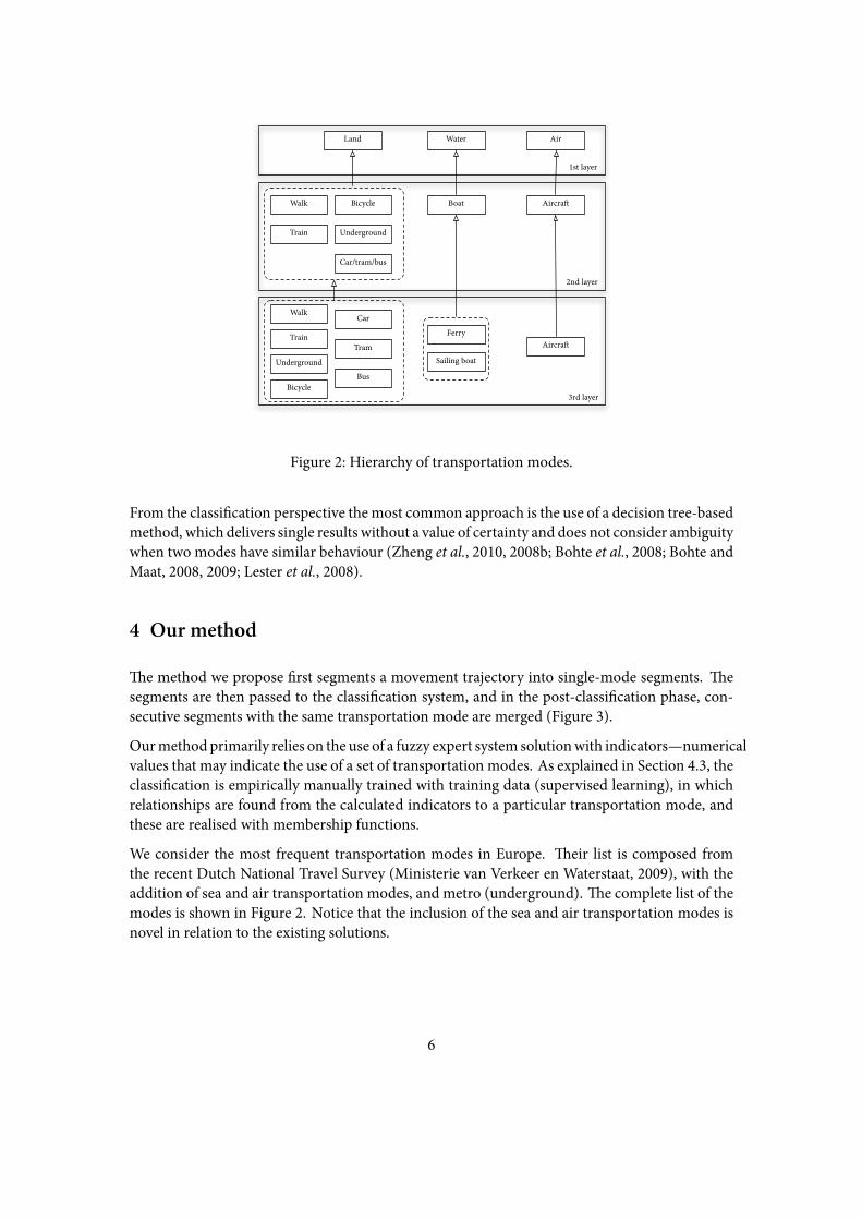
Figure 2: Hierarchy of transportation modes.
From the classification perspective themost common approach is the use of a decision tree-basedmethod, which delivers single results without a value of certainty and does not consider ambiguitywhen two modes have similar behaviour (Zheng et al., 2010, 2008b; Bohte et al., 2008; Bohte andMaat, 2008, 2009; Lester et al., 2008).
4 Our method
The method we propose first segments a movement trajectory into single-mode segments. Thesegments are then passed to the classification system, and in the post-classification phase, con-secutive segments with the same transportation mode are merged (Figure 3).
Ourmethodprimarily relies on the use of a fuzzy expert system solutionwith indicators—numericalvalues that may indicate the use of a set of transportation modes. As explained in Section 4.3, theclassification is empirically manually trained with training data (supervised learning), in whichrelationships are found from the calculated indicators to a particular transportation mode, andthese are realised with membership functions.
We consider the most frequent transportation modes in Europe. Their list is composed fromthe recent Dutch National Travel Survey (Ministerie van Verkeer en Waterstaat, 2009), with theaddition of sea and air transportation modes, and metro (underground). The complete list of themodes is shown in Figure 2. Notice that the inclusion of the sea and air transportation modes isnovel in relation to the existing solutions.
6
For technical reasons, we introduce a new class “Stationary” for all non-moving points. It is notshown in the Figure 2 as it is auxiliary.
As one may anticipate, in a few cases, discerning between a certain subset of the listed modesmay not be possible with a high certainty. For example, buses and cars have similar speeds andacceleration in urban areas and both operate on the same infrastructure. We therefore introducea hierarchy of transportation modes in order to give an accurate result, which is more acceptablethan returning inaccurate or uncertain results. Three layers of transportation modes are gener-ated, and the classification is done separately for each layer.
The first basic layer contains the most general groups: land, sea, and air. In some cases it may becomplex to distinguishing the following groups of modes:
• Bus, tram, and car (similar speed, and use of the same infrastructures);
• Sailing boat and ferry.
In order to avoid the possible errors of the classification system, the second layer contains ag-gregations of some ambiguous modes. Hence, the second layer comprise seven transportationmodes: walk, bicycle, car/tram/bus (a single mode), train, metro, boat (comprises sailing boatand ferry), and aircraft. The third layer has the car, tram and bus modes, and the sailboat andferry models, as separate modes.
4.1 Selection of the indicators
Our research involved testing the usability of a large number of numerical values derived fromthe timestamped positions for the classification of the trajectories. The selection of the indicatorssuitable for the classification for transportation modes resulted in nine values:
• three single values of speeds in the segment: its 95th percentile (the nearly maximumspeed), the mean speed, and the mean moving speed,
• five average proximities of the segment to the infrastructures used by the selected trans-portation modes (railway, tram lines, roads, bus lines, metro lines—with segments that arenot underground where might be GPS reception), and
• the location of the trajectory with respect to water surfaces.
According to other researchers, the acceleration is as a useful indicator (Zheng et al., 2010). How-ever, experiments with our datasets have shown otherwise. Despite the speeds inmost of the GPSdevices being measured accurately with the Doppler effect (Zhang et al., 2006), because of insuf-ficient sampling periods (equal or above five seconds) and because of the variation of speedsbetween the samples, the acceleration was not accurate enough to be used as indicators*. Fur-thermore, in our experience, when considering a larger number of transportation modes theacceleration is no longer an indicator that helps the segmentation process.
*With the use of newer devices with a sampling rate of 1s, acceleration could however be used.
7
On a related note, since the average moving speed is computed from consecutive positions whichmay contain positioning errors, a stationary GPS device will often record low speeds when notmoving at all. This issue is taken into account, it is detected with an algorithm we developed andsuch data is filtered out.
4.2 Concept of the segmentation
As described in Section 2, a GPS track may have been completed with multiple transportationmodes, therefore before any classification first we need to divide it into single transportation-mode segments. The segmentation is done in a two-step process:
1. partition of trajectories to single-journey segments (between two meaningful locations),and
2. segmentation of journeys into single-mode segments.
Although both segmentations technically derive segments, the segments in the first segmentationare referred to as journeys, and the latter simply as segments, as visible in the UML diagram inFigure 1. Once a trajectory is segmented, it is ready for its classification. Therefore, the trajectoriesare segmented before any knowledge of the transportation mode.
4.2.1 Segmentation into journeys between two relevant locations
Different journeys are often separated by a longer interruption in logging the data, caused byeither a signal shortage (individual in a building) or a device turned off. However, regular signalshortage while travelling (e.g. entering a tunnel, or a journey with train) often exhibits the samebehaviour. As a consequence, in addition to the time difference, the distance between the lastknown point before the gap and the first point after the interruption of logging is taken intoaccount. In case of journeys, and not of a signal shortage while moving, the departing point ofthe next journey is usually close to the arrival point of the previous journey. By examining severaldatasets we concluded that most of the journeys are mutually separated by longer period such asa working shift (8-9 hours) or a night, hence they are straightforward to detect and segment.
4.2.2 Segmentation into single-mode segments
The second step of the segmentation is more challenging: the transitions between modes occurmuch faster than transitions between journeys and they require a different approach.
Mountain and Raper (2001) report that the a rapid and sustained change in direction or speedindicates a change ofmode. Therefore, a segmentation algorithmwould require detecting suddenchanges. Although theoretically such approach is plausible, a serious problem arises when dealingwith a transition which does not bear a noticeable change in speed and/or direction.
8
Liao et al. (2006) segmentmulti-modal trajectories by analysing the proximity to potential-transitionlocations such as bus stops. This method presents another interesting use of geodata. However,their approach may have difficulties in areas with dense traffic features (especially in the Nether-lands), where the distance between potential transition points for various modes may be in therange of GPS errors, hence this method is used only partially in order to discern between cars,buses and trams (we elaborate on this in Section 4.4).
Zheng et al. (2010) indicate that a person usually walks or stops during the transition. By examin-ing the test dataset and observing the same behaviour, we choose to second their conclusions andto follow this logic. However, by examining the available data we have noticed that the transitionsoften cause data interruption (signal shortage under the roof in a train station, or entering a bus),hence signal shortages have to be added to the list. They are used as an additional indication fora potential transition.
All stops which are longer than a specific threshold, and also those before a signal shortage, areconsidered as potential transition points. These events indicate that the transportationmodemighthave changed. In determining the threshold, one should consider that over-segmentation of thetrajectories is better than under-segmentation since fast transitions may pass undetected (e.g.exiting a tram/bus, and immediate departure with some other modes).
Since many single-mode trajectories contain stops (e.g. cars stopping for traffic lights), initiallythe trajectory may be segmented into a high number of segments. This is however not a problemsince we merge as post-processing consecutive segments having the same mode (see Figure 3).
AA
B
Transition pointA
B
Potential transitions
Figure 3: All stops and signal shortages in a trajectory are first marked as points of potential tran-sition, and the segments are classified separately. If two adjacent segments have thesame classification outcome, they are merged into one segment.
Each segment is terminated after a stop or signal shortage is encountered. The threshold for adata disruption is set to 30 seconds, while a stop is considered when there is no movement formore than 12 seconds. Since in a stop the position might not be recorded at exactly the sameposition and there might be slight movement, a stop is detected when consecutive points in aninterval of 12 seconds do not have a speed higher than 2 km/h.
Despite our efforts, some cases of very fast transitions cannot be detected, one example beingwhen a person is running to a tram which immediately departs. These cases would require adifferent approach since a shorter thresholdwould compromise other results by creating toomanysegments with just a few points. However, in practice such cases are not frequent.
9
4.3 Concept of the classification
There are various general approaches for building a classification system, as it can be concludedfrom the different existing approaches described in Section 3. In this paper, an expert systemapproach is chosen because of its maturity and because it has been used successfully at solvingother problems (Holzmann et al., 1999; Rearden et al., 2007; Wentz et al., 2008).
An expert system is a software package that can reason through complex situations. It comprisesthe knowledge of an expert in a certain field to provide answers to problems (Buchanan andDuda,1982). It is applicable to specific problems and has been developed to substitute experts. Themosttypical usage of expert systems is in medicine (Grazia, 2006). Expert systems have been used inGIS, for instance in cartography (VanOosterom et al., 2001; Alkemade, 2000; Kotte, 2002), and forarea/object classification of topologically structured topographic data converted from spaghettidata (Van Oosterom, 1999).
Fundamentally, expert systems consist of a knowledge base (evidences e), and an inference pro-cedure (rules), which derive conclusions (hypotheses h): IF e THEN h.
Another important concept in expert systems is (un)certainty, which occurs when one is not ab-solutely certain about a piece of information (Nickles and Sottara, 2009). The degree of certainty,introduced by Shortliffe et al. (1975), is represented by a numerical value CF(h, e), where CF isthe certainty factor, a quantification of the confidence that an expert might have in a conclusionor hypothesis h that s/he has arrived at from an evidence e.
In case that a set of conclusions (hypotheses) derives multiple values of CFs, they should be prop-agated through a reasoning chain, i.e. combined, to obtain one single certainty factor. Severalinference methods had been established for this operation. For instance, in MYCIN (an earlyexpert system developed in the early 1970s at Stanford University), when two CFs are ANDed(conjunctive reasoning), the joint CF is the minimum value of the two (Shortliffe and Buchanan,1975):
CF[A ∩B] = min(CF[A], CF[B])
This approach has the advantage that one CF with the value of 0 may result in a joint CF of 0, i.e.if there is strong evidence that contradicts a hypothesis, other hypotheses with a non-zero CF arediscarded.
The presented concepts appear to be suitable for solving the problem of the classification ofmove-ment trajectories.
In relation to this project, an example of a fact is the mean speed of a trajectory—30 km/h. Byconsidering solely the mean speed of a trajectory, there is suggestive evidence that the value ofthe speed probably represents a car, with e.g. a CF of 1.0.
The fuzzy expert system developed for this paper uses fuzzy logic to derive certainty factors, i.e.fuzzy variables are used to assign certainties to each derived hypothesis. Consider the followingcase of a rule as an explanation of the concept. If the maximum speed in a segment is 118 km/h,
10
from common sense we can build a rule that concludes that the transportation mode could be acar: CFmax.speed
car (118 km/h) = 1.0.
While higher speeds for cars are rare, they should not be discarded as a possibility, since theremight be a possibility that the segment was completed with a car. In order to retain the reasoning,but give it less weight, this is done for instance by assigning a lower CF:CFmax.speed
car (138 km/h) =0.6.
Therefore, the certainty factors in fuzzy expert systems are a function of available evidence: CF =f (e), i.e. membership functions which are empirically defined by investigating travel behaviourfor each transportationmode in the training data, a subset of the test data used for that purpose.
Each available fact should be used for each considered transportation mode (class) in the system.For instance, extending the use of the information of the maximum speed for trains:
CFmax.speedtrain (118 km/h) = 0.4.
Therefore, each rule in the system determines an array of certainty factors, one for each modeconsidered:
IF (max. speed is 118 km/h)THEN CFmax.speed
car = 1.0, CFmax.speedtrain = 0.4, . . .
In case of multiple facts, the final CF is determined as a conjunctive CF since the rules are notused in a particular sequence:
IF (max. speed is 55 km/h)THEN CFmax.speed
tram = 0.85
IF (average proximity to tram network is 4933 m)THEN CF
prox.tram = 0
→ CFtram = min(0.85, 0) = 0
This is done for each mode. From the last example, it is visible that one rule in such system couldcompletely eliminate the possibility of a transportation mode based on only one fact. Therefore,the presented classification system works on the elimination of unlikely modes by assigning themCFs of zero for each evidence that is strongly against a hypothesis.
In order to formalise the presented concepts an overview is given. For each transportation modem (e.g. train) of the N considered modes (modes m1 . . .mn), the classification system containsk membership functions f i
m, where k is total number of indicators (facts) used as the input ofthe classification and i marks the designation of the indicator, e.g. f3
2 or fmax.speedtrain . For each
segment, k indicators i1 . . . ik are calculated (e.g. i3 or iavg.speed) and passed to the respectivemembership functions for each transportation mode (e.g. f3
train(i3), f3car(i3), f3
bicycle(i3), …)from which certainty factors CFi
m = f im(i) are calculated. The total number of the membership
functions and corresponding certainty factors is the product of the number of indicators k withthe number of the considered transportation modes n.
11
After computing the k certainty factors for each transportation mode, the system determinesthe minimum value for each and considers it as a the final CF. The confidence that the mode inquestion was used to complete the classified segment is:
CF11 = f1
1 (i1) CF21 = f2
1 (i2) . . . CFk1 = fk
1 (ik) ⇒ CF1 =min(CF11, . . .CF
k1)
CF12 = f1
2 (i1) CF22 = f2
2 (i2) . . . CFk2 = fk
2 (ik) ⇒ CF2 =min(CF12, . . .CF
k2)
⋮ ⋮ ⋮ ⋮CF1
n = f1n(i1) CF2
n = f2n(i2) . . . CFk
n = fkn(ik) ⇒ CFn =min(CF1
n, . . .CFkn)
The mode with the highest (non-zero) CF may be considered as the result of the classification.
A significant advantage of using certainty values in the results is the possibility of sorting theresults by the value of CF and obtaining alternative results in order to improve the performanceof the classification system.
Theknowledge used for the classification is stored (encoded) separately inmembership functions,and it is explicitly defined. There are numerous types of membership functions. A commonconstruction of a membership is trapezoidal, and it is used in our implementation. Figure 4shows the set of membership functions of the considered modes for the indicator of the nearlymaximum speed.
1T H E S E G M E N TAT I O N A N D C L A S S I F I C AT I O NS Y S T E M
µA
125 1801600
3
1
10010 50 6520 35 80
Figure 1: The membership functions usually overlap. This is an example forthe membership functions for nine modes used in the indicator of thenearly maximum speed (in km/h). The following modes are plotted:car (black), train (yellow), walk (red), bicycle (green), tram (brown),bus (purple), sailing (light blue), ferry (blue), and underground (darkorange). The classes standing and aircraft are left out for aestheticreasons.
i
Figure 4: The membership functions usually overlap. This is an example for the membershipfunctions for ninemodes used in the indicator of the nearly maximum speed (in km/h).The following modes are plotted: car (black), train (dark yellow), walk (red), bicycle(green), tram (brown), bus (purple), sailing (light blue), ferry (blue), and underground(dark orange). The classes stationary and aircraft are left out for aesthetic reasons.
This is also one of the simplest constructions, and it is suitable for this approach. It requires thedefinition of four points, where ≤ x0 and ≥ x3 correspond to a certainty of zero, while betweenx1 and x2 to one. Every value in between the four points is considered as fuzzy. It is importantto note that in this concept the range of the derived values by the MF is [0,1].
The definition of the membership function for each indicator for each transportation mode isdone in a training process also known as trial and error (Section 5.3).
12
4.4 Discerning between similar modes
Classification between bus, car and tram is usually ambiguous because of comparable speeds andbecause they both use the road network. While buses and cars in urban areas operate on thesame roads, when a segment is detected far from the bus network the classification rejects bus asa possibility by assigning a CF of zero. However, in case of the presence of a bus line, but in somecases also a tram line which operates adjacently to the road (on sometimes on the road) and itis in range of GPS errors, the classification is ambiguous and the three classes are assigned withthe comparable CF, e.g. 1.0. This situation is solved by using the locations of the bus and tramstops, and by using the knowledge of the previous used mode. Indeed, if the segment started ata bus/tram station then there is a high probability that the segment was completed by a bus ortram. Thus, the certainty factors for these modes are increased; Figure 5 clarifies this theory. Ifthe new segment is started close to a station, then the corresponding mode gets a CF increasein the subsequent segment. The value is currently put to 0.2 since we have noticed that virtuallyall discrepancies between these three modes in the classification are less than 0.2. The size of thebuffer is currently set to 20 m which compensates the size of the bus/tram stops and the GPSnoise.
Si
Si+ cfbus = . + .cfcar = .
Bus station
Transition point
Bu�er of the station
cftram = .
Figure 5: Injecting certainty factors supplement for segments which commence at a station forbus or tram contribute to the distinction of the modes car, bus, and tram.
However, many tram and bus stops are close to regular car stops (such as traffic lights), whichmay wrongly assign a car segment to a bus or a tram if it was started close to a station. Hence,our method takes into account the knowledge of the previously used transportation mode: if theprevious segment was completed with a car, and ambiguity between car, tram and bus exist, theclass car gets a favourable CF supplement. Bus and tram segments may be possible only when thepreviously used mode was walking.
In addition, buses and tramsmay stop at points outside the buffers of stations (e.g. bridges), whichmay cause the opposite classification. The knowledge of the previously transportation mode isthen taken into account as well.
The disadvantage of this approach is that in rare situations where a person was dropped off from acar directly at a bus or tram station and continued the journey with either a bus or tram are fromthat point wrongly classified as car segments. This is partially solved by analysing the dwell timebetween two segments. If the dwell time after a non-walking segment is longer than a certain
13
threshold and took place in the buffer of a station, then it is assumed that the person was waitingfor a bus/tram, rather than waiting in a car for a traffic light.
4.5 Dealing with disruptions in the data
Signal shortages that cause disruptions in the acquisition of data (i.e. gaps) are frequent and hardto handle since we are dealing with the classification of non-existing data. As noted, we considerdata as missing when no samples are recorded for more than 30 s. The problem is complex sincethere are numerous cases, one example is that the transportationmode could have changed duringthe disruption.
Resolving the gaps requires investigating many possible cases that occur in practice. In additionto these problems, this method takes advantage of gaps, since the metro mode does not have anyreception, and it is detected by the disruption of signal in between entrances to the two metrostations, similar to the methods of Stopher et al. (2008) and Shalaby et al. (2006).
The following distinct cases account for most, if not all occurrences of gaps, and their reconstruc-tion was developed and implemented in the prototype. All cases are depicted in Figure 6.
Since the points are not sampled, we must guess what happened during the gap. The distancebetween the two adjacent recorded segments is known, along with the time difference. Fromthese, the average distance may be computed, although this is rather a rough approximation dueto the potential sinuosity of the travelled path. As one might suggest, proximity to the stationsfor certain modes are available for the points on the edge of the gap. Although it is possible totake into account the proximity to the stations, these cases have something more in common—they occur on the network of each corresponding mode. Hence, instead of stops, the location ofnetworks is used, which are already available from the preprocessing procedure.
Before each disruption in the data, the system stores the classification result of the precedingsegment, and the distance from the last known point to all considered infrastructures. This isalso done for the first point after the gap.
The reasoning system analyses the infrastructures from the buffers of the boundary points ofthe segments (last recorded point in the previous segment and first in the subsequent segment).If two infrastructures match (e.g. if both points fall in a buffer), then the corresponding mode isassigned. This is especially useful for undergroundmodes since it is the only way to classify them.Indeed, some metros have part of their networks on the surface, but almost always involve datamissing time intervals.
In case of the match of multiple infrastructures, the average speed of the gap and the knowledgeof the previous transportation mode prevails. If neither conditions are met, the system analysesthe average speed of the gap, and the average speed of the first 20 points of the next segment. Ifeither speed is higher than 300 km/h, the gap is marked as ‘air’.
The value of 20 points in the following segment was taken into account in order to preserve thetravel behaviour of the segment in the portion closer to the gap. This is useful in cases where
14
Car Car Car
(a) “Regular” gaps where the mode was not changed.
Bike Train Walk
(b) The whole segment done with another mode is not recorded.
BikeTrain WalkTrain
(c) The first transition is recorded, but not the rest of the segment and the secondtransition.
BikeTrain WalkTrain Train
(d) Neither of the transitions is detected, but a small fragment of the segment isrecorded in between.
Bike WalkTrain
BikeWalk
(e) Signal shortage occurs during both transitions, the mode is not recorded, andthe disruptions exist in the earlier and next segments.
BikeBus WalkTrain
(f) Signal shortage occurs during both transitions, the mode is not recorded, andthe disruptions exist in the earlier and next segments.
Figure 6: General cases of data interruption.
15
the subsequent segment is relatively long and during its course exhibits behaviour which can bedifferent than in its part closer to the previous segment (e.g. much higher speed).
This solves the cases (a), (b), (c), (d) shown in Figure 6 by a unified approach. The method is alsouseful in segments where only fragments of data are available.
Case (e) is resolved only in instances where the time difference and distance to the occurredtransition is small. In other cases the segment is marked as unknown as it involves too muchambiguity. The same applies for (f) which is a case that cannot be solved even with human inter-vention.
Another specific case that could not be solved is that if a person lost GPS signal while board-ing a ferry, and reappeared after the segment was finished. The sea mode could not be resolvedsince both boundary points fall onto land. Reasoning that the person crossed a water polygonin between requires complex GIS operations (and there is always the possibility that the personcrossed a bridge).
Althoughmachine reasoning in signal shortages is complex, we have obtained satisfactory resultsand “repaired” the available datasets. We believe that the presentedmethod of classifying deficientand broken data is a contribution in this field.
5 Implementation
Aprototype, implemented inPython, was created in order to test the presented approach. Figure 7depicts the workflow of the implementation.
(x,y,z,t)
Geodata
Calculate indicators
(x,y,z,t, indicators) Segmentation
(x,y,z,t, segment_id)
Classified points and segments
1) Raw movementdata (trajectories)
2) OpenStreetMap
3) Empiricalrelationships
input:
output:
Classi!ed andsegmented data
1st step(preprocessing)
Preprocesseddata 2nd step
Segmenteddata
3rd step
(x,y,z,t, mode)
Classi!eddata
Merging segments
4th step
Membership functions
Classification
Figure 7: Flowchart of the implementation of the prototype.
Raw movement datasets in form of timestamped positions (x, y, z, t) are imported in a database(PostgreSQL with PostGIS in our case), and are preprocessed for the required indicators (first
16
step). Geodata required for the calculation of the indicators come from the OpenStreetMapproject (described in Section 5.1) and have been stored in the same database. To each point isattached a series of indicators which are later used in the classification. Afterwards the data issegmented (second step) into single-mode trajectories in single-journeys (Section 4.2), whichare then passed to the classification system. The classification system, aided by the membershipfunctions and certainty factors (Section 4.3), classifies each point for the transportation mode(third step). The classified segments are then finally merged with adjacent segments of the sameclass (fourth step) resulting in the segmented and classified trajectories.
In order to test the developed method and the prototype two large movement datasets wereused:
• the data from the survey conducted in the Netherlands by Bohte andMaat (2009) as part ofa travel behaviour study focused on residential choice. This dataset contains 7-day move-ment logs of a thousand respondents collected with a handheld GPS logger with a SiRF-StarII chip, with an average sampling period of 6.5 s. The data have been classified in aninterpretation-validation process in which the system first made a preliminary basic seg-mentation and classification, after which the data have been checked and corrected by therespondent in a web-based questionnaire. Bohte and Maat (2009) are interested in remov-ing or shorten the validation process by improving and automatizing the segmentation andclassification process, which is one of the motives for our research. The data corrected bythe respondents may be used as a reference for experiments and for validation.
• The manually classified data from the project of Van der Spek et al. (2009) from the De-partment of Urbanism, Faculty of Architecture, Delft University of Technology is used aswell. The project concentrates on collecting data on various types of pedestrian movementin city centres. It addresses the topic of improving city centres for pedestrians, especiallyfor shoppers and tourists (Van der Spek, 2010). This dataset has been collected with deviceswith a newer and more sensitive chip (SiRFStarIII), with a sampling period of 5 s.
Notice that for all the GPS tracks, we used the speed as calculated by the receivers (using theDoppler effect). Also, it was important to check the robustness of the method with data ob-tained with various devices of different sensitivity and technology (different frequency of signalshortages and accuracy). Thus, we downloaded additional movement data from the internet (e.g.OpenStreetMap raw logs for which the transportation mode was known), and from various de-vices that we used (mobile phones, and with handheld GPS devices of different production yearsand manufacturers).
In total, the available data contains 17.5 million GPS points in trajectories longer than half of amillion kilometres, well covering the considered transportation modes and various movementscenarios required for testing the robustness of the method for different situations.
As an impression of the available datasets and their size, Figure 8 shows the Dutch city Amers-foort “mapped” from the available movement data. Frequently used paths (e.g. highways) can beobserved by the aggregation of multiple points (i.e. thicker lines).
17
Figure 8: Visualisation of an excerpt of the GPS data used in the implementation (Amersfoort,the Netherlands) and its classification. The left side of the Figure represents a collectionof rawGPS points, while the right side represents the visualisation of classified GPS dataof the same spatial extent with different colours accounting for different transportationmodes. Red represents walking, while green and blue are for bicycles and cars, respec-tively. Train is represented in yellow, visible on the diagonal railway.
After the preprocessing (calculation of the indicators), the data are ready for segmentation, wherethe movement archive is segmented between all stops, and passed to the classification system.
It should also be said that the definition of the membership functions, the empirical relationships,are stored in a separate XML file which enables the extension of the prototype for additionalindicators or transportation modes.
5.1 OpenStreetMap
For geographical data, we chose to use the data from the OpenStreetMap (OSM) project becausethey are available for free usage, they contain all the needed features (e.g. bus infrastructure, atleast in the Netherlands) and they have a good coverage (at least in Western Europe). OSM is acollaborative project to create a free editable map of the world, and one can download and freelyuse the data. Several studies have looked at the quality of the OSM data in different countriesin Europe, see for instance Haklay (2010) for the UK, Girres and Touya (2010) for France andZielstra and Zipf (2010) for Germany. We are not aware of any such study in the Netherlands,but the dataset is certainly up-to-date and accurate enough since several high-quality datasets ofthe Netherlands have been recently donated to the OSM project. First, the buildings are coming
18
from the topographic map (Top10NL)†, and second the roads are very accurate since in 2007the Dutch mapping company ‘Automotive Navigation Data’ donated their entire street map of theNetherlands‡. Other useful information (e.g. location of bus stops, of airports, of the railways) isalso continually added to the OSM database.
The data are organised separately into geometry (polylines) and corresponding attributes (tags).By contrast, most GISs use Simple Features to store geographical objects, so we had to convertthe datasets to that format before being able to to calculate indicators from it.
5.2 Import and preprocessing of the trajectories
Movement data are usually stored in the GPX format (GPS exchange format), an example of apoint stored in the GPX format is shown in the continuation:
The trajectories are imported and stored in the database point by point, and are immediatelypreprocessed for the different indicators. The computation of some indicators is derived fromother indicators (e.g. the maximum speed is calculated after the speeds at all points are derived),hence the preprocessing is done in multiple passes.
5.3 Training of the system
In order for the system to performwell, the proper values for defining theMembership Functions(MF) for every transportation mode have to be defined. Currently this is done in an iterative pro-cess starting with common senses values for bikes, cars, trains, etc. These values for the MF areencoded in an XML file and the system then classifies the segments. This automatic classificationis then compared to the ‘ground truth’ of the dataset (the results classified by the respondents)and a score is assigned based on the similarity between the automatic and the manual classifica-tion. If needed the MF values are adjusted and a new iteration is executed until the results are
†http://wiki.openstreetmap.org/wiki/3dShapes and https://rejo.zenger.nl/inzicht/aanvullende-informatie-over-het-3d-shapes-bestand (in Dutch).
satisfactory; e.g. the score is above 95%. Note that each iteration is quite expensive as new MFsimply computing again the indicators for the segments and based on the new indicator valuesthe rules are applied for classification. The next excerpt shows a fragment of XML file with MFvalues:
i.e. the four values of the MF of mean speed for the transportation mode walking (3rd layer) are0, 1, 8, and 10 km/h.
What is actually going on is a search process to optimal values for the MF functions. For eachtransport mode there is one MF function described by values. Currently this is a manual trial-and-error process based on analysing the errors.
The end results are extremely sensitive to the determination of the MF parameters. When usinga dataset which is not homogenous, many trade-offs should be taken into account due to largedifferences and possibilities in mode behaviour.
However, this process could also be automated by considering it as a search problem to optimizethe score in the high-dimensional space of all values ofMF. In principle all steps can be automated:setting four MF values, computing indicators, assigning classification and finally computing theoverall score. Hence, we could use one of the well know search/optimization algorithms suchas hill climbing, simulated annealing, genetic algorithm, etc. (Russell, 2003; S. Kirkpatrick andVecchi, 1983; Michalewicz, 1996). As each iteration is relatively expensive, we could try to use asubset of the manual classified segments and optimize for this subset. If good results are obtainedwe can try these MF values for all manual classified segments. If results are still good then thesubset was representative; if the score is not good the subset was not representative. In such a casewe should either use a different segment or more segments (e.g. if not all cases were sufficientlyrepresented).
One last warning: the manual classified segments are now considered as the ground truth. Forour data this was not really true. We inspected the differences between the manual and the auto-mated classifications and it could be observed that theymade about the equal number ofmistakes(but different ones); for instance many segments of different public transport modes were clas-sified as one segment, and in general short segments were often not noted. This is somethingthat automatic training (optimizing) of the system can not improve (as it considers the manualclassified data as truth and tries to get as close as possible to these classification).
6 Experiments and validation
In order to assess the quality and the applicability of the developed segmentation and classificationmethod, unbiased validation methods have been applied. It was decided to use two different
20
large test datasets for the validations: implying different types of GPS receivers (both new andold), different regions, different timeframes, different sampling periods, and different and non-related organisers of the collection of the involved GPS traces. As explained in Section 5 thesetwo datasets are from the research projects of (1) Bohte and Maat (2009) and (2) Van der Speket al. (2009). The size of the datasets and the variety of all kinds of different movement situationsis a guarantee for robust validation.
The datasets have been manually and independently classified within the scope of the originalresearch projects. This classification will now be used as reference material, i.e. ‘ground truth’, forour developed automated approach. There are a few difficulties when comparing the results:
• the segments are not segmented exactly at the same transitions points (so one should acceptsmall differences here),
• our new approach has a more refined classification scheme (hierarchy of transportationmodes, see Fig. 2), and
• the manual classification taken as ’ground truth’ might contain errors.
In order to copewith the abovementioned validation problemswe took the following approach:
• we remapped our refined classification in the validation to the rougher classification oforiginal test data (our classes x1, x2, . . . to class y1 of the reference classification, e.g. busand tram are grouped together for the class bus/tram that is defined in the test dataset whichwas further checked),
• for comparable classes, we collected statistics on the amount of overlap between the twoclassifications at point level—this resulted in respectively y1p , y2p , y3p agreements and over-all yp of 91.6 %, and
• finally, the individual cases were inspected further where there was a large number of se-quential points in a GPS trace that were classified differently. From this inspection (cases)it turned out that there was about an equal amount of manual error and automated errors,i.e. about half of the 8.4% ‘error’ was indeed correct (4.2%), resulting in an overall scoreof about 95% (a little lower than 95.8% as there is a small changes that both manual andautomated classification are wrong and equal, though we did find no indication for this).Some transportation modes in various situations have been classified with a 100% accu-racy, e.g. cars on journeys longer than a few kilometres. When taking into account alsothe alternative result with the second highest CF, the accuracy was nearly 100%, which isa clear advantage over methods that do not determine values of certainties.
The right side of the Figure 8 shows the GPS data in the spatial extent shown on the left side ofthe same Figure classified by our fully automated classification and this reinforces the confidencein the above stated positive results of the validation method.
A significant difference between the accuracy of the movement data obtained with relatively oldand new devices has not been found. Thanks to the presented approaches, which takes into ac-count the signal shortages, the accuracy is not affected by the deficiencies found in data acquired
21
with older devices. The method can be seen as a worst case scenario where the results can onlybe improved when newer receivers are used.
The developed method was further checked on various smaller datasets collected by us and oth-ers retrieved from the internet for tests with the data acquired with different sampling periods,on a different location and with different GPS devices, as further explained in Biljecki (2010).The segmentation and classification results obtained with the presented automated method arecomparable to the above presented findings.
The results may be further improved when optimising the knowledge (membership functions)and using datasets from single sources which contain an uniform behaviour and smaller geo-graphic extent.
7 Discussion and Future Work
The work described in this paper has been initiated by the need of a classification solution forthe data acquired for the travel behaviour study conducted by the Department of Urban andRegional Development (Bohte and Maat, 2009) and the Department of Urbanism (Van der Speket al., 2009) at TU Delft. We have described an algorithm, we have implemented it, and we havevalidated our results. Their dataset is now classified with a significantly higher accuracy than theexisting (semi-manual) method that had been originally used (since we introduced automaticsegmentation of the trajectories), and we take into account ten different transportation modes.Apart from travel behaviour research, we believe our method and our prototype is useful in otherdisciplines since it can be easily extended with new transportation modes (one simply has todefine the MFs for all the indicators, i.e. speed, proximity to a certain infrastructure) and thecurrent MFs can also be modified so that they are more realistic for a given country (we have setthem up for the Netherlands here). Moreover, themethod is universal and we had shown it worksfor movement data collected with any relatively modern GPS device.
Although it is very difficult to take into account all possible cases in the real-world, the prototypeyielded satisfactory results, especially in the segmentation and classification of data containingnoise or having a small number of samples.
The errors are usually not caused by the imperfection of the system, rather by specific situationswhose modelling would be either complicated or would impair the existing classification perfor-mance. We believe that the development of a system that takes into account virtually all possiblesituations in movement may not be possible.
One reasonwhywe obtained better results than previous attempts is thatwe rely heavily on the useof geographical data for the indicators, which permits us to resolve gaps, ambiguity between car,bus and tram, and to enrich the trajectories with additional information about the transportationmodes. Without geographical data this would not be possible. A few years ago it would have beenunthinkable to have (free) access to such datasets, but OpenStreetMap solves that problem andwe believe that the quality and coverage of the data uploaded to their servers will only increase inthe next year (this is certainly our experience with the data in the Netherlands).
22
Ourmethod distinguishes between ten transportationmodes, which is to the extent of our knowl-edge, more than any othermethods. Although a lot of overlapping characteristics betweenmodesexist, with a careful selection of the indicators andmodelling of correspondingmembership func-tions the accurate classification of a large number of modes was made possible. Discerning be-tween car, bus, and tram is done thanks to a developed technique of injecting supplementaryconfidences based on previous knowledge, which is a novelty. However, there are still cases thatwe cannot really solve, for instance the difference between bicycles and scooters. In the Nether-lands these two modes use primarily the cycling paths, and travel at similar speeds; we tried touse the acceleration to differentiate them but because of the noise in the data that proved unsuc-cessful. We hope that with newer GPS units that problem will be solved.
For future work, we plan to improve the prototype by training the system with more datasetscoming from newer and better GPS units. We plan to allow users to upload their own GPS logsto a website and let them manually classify their trajectories; that knowledge could then be usedto improve our method. Users would also be able to upload their GPS logs and get back seg-mented and classified trajectories, in aKMLfile for instance. We also plan on usingmore auxiliarydatasets, such as the type of a road or speed limit. For instance, if it is known that in the Nether-lands most of the traffic jams occur on highways, then the classification system may take that factinto account and compensate the speed on such locations (depending on the time of the day).The number of lanes of a road, which is conceptually available in OSM but often not acquired,could be used to alter the MF for the proximity to a road (i.e. a wider road would require a widerMF). Finally, we think that a better classification could be obtained if data about the users wereused. Indeed, since a user’s trajectory ordinarily contains repetitive journeys, not only in spacebut also in time and usually with the same transportation mode(s) (e.g. every-day commuting),historical user data may be used to improve the classification in uncertain situations. Similarly,in movement research surveys, extensive data from numerous respondents is often available. Bymodelling patterns and transportation modes from a group of similar movements, it may be pos-sible to facilitate the classification by searching for a similar trajectory in the database and assignthe transportation mode from existing trajectories (classified patterns) in the database.
Acknowledgements
The authors would like to thank the Department of Urban and Regional Development and theDepartment of Urbanism at the Delft University of Technology for sharing the test datasets.
ReferencesAlkemade, I., Beeldschermkartografie ten behoeve van multi-bron internet GIS. Master’s thesis,
Delft University of Technology, 2000. .
Asakura, Y., Tanabe, J., and Lee, Y., 2000. Characteristics of positioning data formonitoring travelbehaviour. In: 7th World Congress on Intelligent Transport Systems, Torino, Jan., p. 8.
23
Axhausen, K., et al., 2004. 80 weeks of GPS-traces: Approaches to enriching the trip information.In: Transportation Research Board 83rd meeting, Jan., p. 28.
Biljecki, F., Automatic segmentation and classification of movement trajectories for transporta-tion modes. MSc Geomatics, GIS technology group, Delft University of Technology, theNetherlands, 2010. .
Bohte,W. andMaat, K., 2008.Deriving andValidatingTripDestinations andModes forMulti-dayGPS-based Travel Surveys: An Application in the Netherlands. In: Transportation ResearchBoard 87th Annual Meeting, p. 17.
Bohte, W. and Maat, K., 2009. Deriving and validating trip purposes and travel modes for multi-day GPS-based travel surveys: A large-scale application in the Netherlands. Transport ResC-Emer, 17 (3), 285–297.
Bohte, W., Maat, K., and Quak, W., 2008. A method for deriving trip destinations and modes forGPS-based travel surveys. In: J. Van Schaick and S. Van der Spek, eds. Urbanism on Track.IOS Press, chap. 10, 129–145.
Bricka, S. and Bhat, C., 2006. Comparative Analysis of Global Positioning System-Based andTravel Survey-Based Data. Transportation Research Record: Journal of the Transportation Re-search Board, 1972, 9–20.
Buchanan, B.G. and Duda, R.O., 1982. Principles of Rule-Based Expert Systems. In: M. Yovitz,ed. Advances in Computers., Vol. 22 Academic Press, New York, p. 62.
Byon, Y.J., Abdulhai, B., and Shalaby, A., 2009. Real-Time Transportation Mode Detection viaTrackingGlobal Positioning SystemMobile Devices. Journal of Intelligent Transportation Sys-tems, 13 (4), 161–170.
De Boer, A., Analysis of GPS logs for algorithm design of movement behavior studies. , 2008. ,Technical report, Delft University of Technology.
Dodge, S., Weibel, R., and Forootan, E., 2009. Revealing the physics of movement: Comparingthe similarity of movement characteristics of different types of moving objects. Computers,Environment and Urban Systems, 33 (6), 419–434.
Draijer, G., Kalfs, N., and Perdok, J., 2000. Global Positioning System as data collection methodfor travel research. Transportation Research Record: Journal of the Transportation ResearchBoard, 1719, 147–153.
Girres, J.F. andTouya, G., 2010.Quality Assessment of the FrenchOpenStreetMapDataset.Trans-actions in GIS, 14 (4), 435–459.
Gonzalez, P., et al., 2010. Automatingmode detection for travel behaviour analysis by using globalpositioning systems-enabled mobile phones and neural networks. In: IET Intelligent Trans-port Systems, Vol. 4, Jan., 37–49.
Grazia, C.U., Introduzione ai sistemi esperti. , 2006. , Technical report, Sistemi di elaborazionedelle informazioni, Dipartimento di Scienze, Università degli Studi ”Gabriele D’Annunzio”.
24
Haklay, M., 2010. How good is volunteered geographical information? A comparative study ofOpenStreetMap and Ordnance Survey datasets. Environment and Planning B: Planning andDesign, 37 (4), 682–703.
Holzmann, C.A., et al., 1999. Expert-system classification of sleep/waking states in infants. Med-ical and Biological Engineering and Computing, 37 (4), 466–476.
Kotte, I., Een kartografisch expert systeem ten behoeve van presentatie van gedistribueerde ge-ografische informatie. Master’s thesis, Delft University of Technology, 2002. .
Lester, J., et al., 2008. MobileSense - Sensing Modes of Transportation in Studies of the BuiltEnvironment. In: International Workshop on Urban, Community, and Social Applications ofNetworked Sensing Systems - UrbanSense08, Oct., p. 5.
Liao, L., et al., 2006. Building personal maps from GPS data. Annals of the New York Academy ofSciences., Vol. 1093, 249–265.
Liao, L., et al., 2007. Learning and inferring transportation routines. Artificial Intelligence, 171,311–331.
Maat, K. and Timmermans, H., 2006. Influence of Land Use on Tour Complexity: A Dutch Case.Transportation Research Record: Journal of the Transportation Research Board, 1977, 234–241.
McGowen, P. andMcNally, M., 2007. Evaluating the Potential To Predict Activity Types fromGPSand GIS Data. In: Transportation Research Board 86th meeting, Jan., p. 21.
Ministerie van Verkeer en Waterstaat, Mobiliteitsonderzoek Nederland. Het onderzoek. Techni-cal report, 2009. .
Mountain, D. and Raper, J., 2001. Modelling human spatio-temporal behaviour: a challenge forlocation-based services. In: GeoComputation - Brisbane, p. 9.
Nickles, M. and Sottara, D., 2009. Approaches to Uncertain or Imprecise Rules - A Survey. In:G. Governatori, J. Hall and A. Paschke, eds. Rule Interchange and Applications., Vol. 5858 ofLecture Notes in Computer Science Springer Berlin / Heidelberg, 323–336.
Ranjitkar, P., et al., 2002. Car-Following Experiments Using RTK GPS and Stability Characteris-tics of Followers in Platoon. In: Proceedings of 7th International Conference on Application ofAdvanced Technologies in Transportation Engineering, Vol. 245, Jan., 608–615.
Rearden, P., et al., 2007. Fuzzy Rule-Building Expert System Classification of Fuel Using Solid-Phase Microextraction Two-Way Gas Chromatography Differential Mobility SpectrometricData. Analytical Chemistry, 79 (4), 1485–1491.
Reddy, S., et al., 2008. Determining transportation mode on mobile phones. In: 12th IEEE Inter-national Symposium on Wearable Computers, 25–28.
25
Reddy, S., et al., 2010. Using Mobile Phones to Determine Transportation Modes. ACM Transac-tions on Sensor Networks, 6 (2), 13–40.
S. Kirkpatrick, C.D.G. andVecchi, M.P., 1983. Optimization by SimulatedAnnealing. Science, 220(4598), 671–680.
Schüssler, N. and Axhausen, K.W., 2009. Processing Raw Data from Global Positioning SystemsWithout Additional Information. Transportation Research Record: Journal of the Transporta-tion Research Board, 2105 (4), 28–36.
Shalaby, A., et al., 2006. New Tools for GPS-based Travel Surveys and TrafficMonitoring. In: NewFrontiers in Transport Systems, p. 33.
Shortliffe, E. and Buchanan, B.G., 1975. A model of inexact reasoning in medicine.MathematicalBiosciences, 23 (3-4), 351–379.
Shortliffe, E., et al., 1975. Computer-based consultations in clinical therapeutics: explanation andrule acquisition capabilities of the MYCIN system. Computers and biomedical research, 8,303–320.
Spaccapietra, S., et al., 2008. A conceptual view on trajectories. Data & Knowledge Engineering,65, 126–146.
Stopher, P., et al., Deducingmode and purpose fromGPS data. , 2008. , Working paper ITLS-WP-08-06, Institute of transport and logistic studies, TheAustralian Key Centre in Transport andLogistics Management, The University of Sydney.
Stopher, P., FitzGerald, C., and Zhang, J., 2007. Search for a global positioning system device tomeasure person travel. Transport Res C-Emer, 16, 350–369.
Van der Spek, S., et al., 2009. Sensing Human Activity: GPS Tracking. Sensors, 9, 3033–3055.
Van der Spek, S., 2010. Tracking Tourists in Historic City Centres. In: U. Gretzel, R. Law andM. Fuchs, eds. Information and Communication Technologies in Tourism 2010. Proceedings ofthe International Conference in Lugano, Switzerland, February 10–12, 2010 Springer Vienna,chap. 5, 185–196.
Van Oosterom, P., 1999. Rule-based Polygon Classification of Topologically structured Topo-graphic Data converted from Spaghetti Data. In: Computational Cartography, Dagstuhl-seminar, 19-24 october 1999, Oct.
Van Oosterom, P., et al., 2001. Multi-Source Cartography in Internet GIS. In: Proceedings 4thAGILE Conference, Brno, April., 562–573.
Verbree, E., et al., 2005. GPS-monitored itinerary tracking: Where have you been and how didyou get there?. Geowissenschaftliche Mitteilungen, 74, 73–80.
Wentz, E.A., et al., 2008. Expert system classification of urban land use/cover for Delhi, India.International Journal of Remote Sensing, 29 (15), 4405–4427.
26
Wolf, J., 2000. Using GPS data loggers to replace travel diaries in the collection of travel data.Thesis (PhD). Georgia Institute of Technology.
Wolf, J., Guensler, R., and Bachman, W., 2001. Elimination of the travel diary: Experiment toderive trip purpose from Global Positioning System Data. Transportation Research Record:Journal of the Transportation Research Board, 1768, 125–134.
Zhang, J., et al., 2006. On the relativistic Doppler effect for precise velocity determination usingGPS. Journal of Geodesy, 80, 104–110.
Zheng, Y., et al., 2008a. Understanding mobility based on GPS data. In: Proceedings of ACM con-ference on Ubiquitous Computing (UbiComp 2008), Seoul, Korea, 312–321.
Zheng, Y., et al., 2010. Understanding Transportation Modes Based on GPS Data for Web Appli-cations. ACM Transaction on the Web, 4 (1), 1–36.
Zheng, Y., et al., 2008b. Learning transportation mode from raw GPS data for geographic ap-plications on the web. In: International World Wide Web Conference: Proceeding of the 17thinternational conference on World Wide Web, Apr., 247–256.
Zielstra, D. and Zipf, A., 2010. A Comparative Study of Proprietary Geodata and VolunteeredGeographic Information for Germany. In: Proceedings 13th AGILE International Conferenceon Geographic Information Science, Guimarães, Portugal.