TRANSPORTATION SYSTEM MODELING AND APPLICATIONS IN EARTHQUAKE ENGINEERING

BY

LIANG CHANG

DISSERTATION

Submitted in partial fulfillment of the requirements for the degree of Doctor of Philosophy in Civil Engineering

in the Graduate College of the University of Illinois at Urbana-Champaign, 2010

Urbana, Illinois

Doctoral Committee:

Professor Amr S. Elnashai, Co-Chair Professor Billie F. Spencer Jr., Co-Chair Assistant Professor Junho Song Assistant Professor Yanfeng Ouyang

ii

ABSTRACT

Transportation networks constitute one class of major civil infrastructure systems that is a

critical backbone of modern society. Physical damage and functional loss to transportation

infrastructure systems not only hinder everyday societal and commercial activities, but also

impair post-disaster response and recovery, leading to substantial socio-economic consequences.

Therefore, understanding and modeling the disastrous impact on the transportation

infrastructures and the corresponding changes of travel patterns under extreme events are vital

for stakeholders, emergency managers, and government agencies to mitigate, prepare for,

respond to, and recover from the potential impact.

This research is aimed at developing a systematic approach for risk modeling and disaster

management of transportation systems in the context of earthquake engineering. First, by

employing the performance metrics that are suited for immediate post-disaster response, this

dissertation explores efficient methodologies to maximize the overall system functionality and

the benefit of mitigation investment for transportation infrastructure systems. Furthermore, the

regions potentially unreachable after a damaging earthquake are identified promptly by using

network reachability algorithms that provide essential information for rapid emergency response

decision-making. Lastly, an integrated simulation model of travel demand that accounts for

damage of bridge and building structures, release of hazardous materials, and influences of

emergency shelters and hospitals, is developed to approximate the “abnormal” post-earthquake

travel patterns and evaluate the functional loss of the transportation systems.

This study extends the understanding of disaster management of transportation

infrastructure systems. The methodologies developed in this study have the following

significance: (i) help leverage available mitigation resources to improve the disaster resilience

iii

and functionality of transportation infrastructure systems; (ii) enable emergency response and

recovery teams to rapidly identify and evaluate the performance of optimal routes for emergency

ingress and egress; (iii) accurately estimate traffic congestion under extreme events; and (iv)

provide important insights necessary to make decisions on protecting these systems to meet the

needs of current and future generations.

iv

ACKNOWLEDGMENTS

This work could not have been completed without the members of my doctoral committee.

First, I wish to express my sincere gratitude to my advisors, Professor Amr S. Elnashai and

Professor Billie F. Spencer Jr. for their continuous support and encouragement. I feel privileged

and would like to thank them for providing insight in all aspects of this research and nurturing

my academic and professional development through their mentorships. I would also extend my

gratitude to my advisory committee, Professor Junho Song and Professor Yanfeng Ouyang for

taking their time to review this work and to provide advice, criticism, and recommendations.

Many other people contributed to the development of this research. Particularly, I would

like to acknowledge Dr. YoungSuk Kim of EQECat Inc., and Dr. JongSung Lee of the National

Center for Supercomputing Applications (NCSA) for their expertise and support. I sincerely

appreciate Professor Travis S. Waller of the University of Texas at Austin for his advice on

transportation modeling, and Mr. Timothy Gress for the support and help in the acquisition of

necessary transportation data. I would like to gratefully thank Professor Tschangho John Kim,

Professor Zhenghong Tang of University of Nebraska–Lincoln, and Professor Yang Zhang of

Virginia Polytechnic Institute and State University, for their valuable discussions and assistances.

I would also like to thank many who have provided valuable information and practical

insight. These people include but not limited to: Dr. Eugene Schweig (U.S. Geological Survey),

Professor Chris Cramer (University of Memphis), Professor Reginald DesRoches (Georgia

Institute of Technology), Mr. Steve Besemer (Missouri State Emergency Management Agency),

Mr. Richard Bennett (Missouri Department of Transportation), Mr. Phillip Anello (Illinois

Emergency Management Agency), Mr. Scott Clarke and Mr. Omar Abou-Samra (American Red

Cross), Mr. Jim Wild, Ms. Lubna Shoaib, and Mr. Johnnie Smith (East-West Gateway Council

v

of Governments), Mr. Richard Bowker (Memphis Light, Gas and Water Division), Mr. Greg

Duncan, Mr. Terry Leatherwood, and Mr. Wayne Seger (Tennessee Department of

Transportation), Ms. Martha Lott and Mr. Pragati Srivastava (Memphis Urban Area Metropolitan

Planning Organization).

I am grateful to my fellow students in the Mid-America Earthquake Center, to my friends at

the University of Illinois at Urbana-Champaign, and especially to Lisa Cleveland, Can Unen,

Joshua Steelman, Young Joo Lee, Wen Hee Kang, Jun Ji, Zhongzhuo Li, Sheng-Lin Lin, Oh-

Song Kwon, Fan Peng, Xiaopeng Li, and Wei Xu. Finally, I owe my tremendous thanks to my

family for their unconditional love and steady encouragement through the course of my studies.

The work was supported by the National Science Foundation under the Award Number

EEC-9701785 through the Mid-America Earthquake Center. Additional support was provided by

the Federal Emergency Management Agency through a grant from the U.S. Army Corps of

Engineers (Army W9132T-06-2).

vi

TABLE OF CONTENTS

LIST OF FIGURES .................................................................................................................VIII

LIST OF TABLES ....................................................................................................................... X

CHAPTER I INTRODUCTION .............................................................................................. 1

1.1 BACKGROUND...................................................................................................................... 1 1.2 CHALLENGES AND ISSUES .................................................................................................... 2 1.3 OBJECTIVES AND EXPECTED IMPACT OF RESEARCH............................................................. 4 1.4 SCOPE .................................................................................................................................. 6 1.5 ORGANIZATION OF DISSERTATION ....................................................................................... 6

CHAPTER II LITERATURE REVIEW.................................................................................. 8

2.1 SEISMIC RISK ASSESSMENT OF INFRASTRUCTURE COMPONENTS......................................... 8 2.1.1 Hazard Definition............................................................................................................ 9 2.1.2 Structural Vulnerability and Functionality...................................................................... 9 2.2 PERFORMANCE MODELING AND EVALUATION OF TRANSPORTATION SYSTEMS................. 14 2.2.1 Travel Delay Cost.......................................................................................................... 15 2.2.2 Network Flow Capacity ................................................................................................ 30 2.2.3 Reliability of Network Reachability ............................................................................. 31 2.3 HAZARD MITIGATION FOR TRANSPORTATION SYSTEMS .................................................... 36 2.3.1 Component-Level Approaches...................................................................................... 37 2.3.2 Network-Level Approaches .......................................................................................... 39 2.4 SUMMARY.......................................................................................................................... 42

CHAPTER III NETWORK-BASED PERFORMANCE MODELING FRAMEWORK . 45

3.1 METHODOLOGICAL FRAMEWORK ...................................................................................... 45 3.2 THE NEW MADRID FAULT ZONE AND HAZARD CHARACTERIZATION ................................ 47 3.3 BRIDGE DAMAGE ASSESSMENT ......................................................................................... 48 3.4 BRIDGE DAMAGE-FUNCTIONALITY RELATIONSHIP............................................................ 52 3.5 NETWORK ANALYSIS OF TRANSPORTATION SYSTEMS ....................................................... 53 3.5.1 Network Flow Capacity ................................................................................................ 54 3.5.2 Reliability of Network Reachability ............................................................................. 55 3.5.3 Travel Delay Cost Metric.............................................................................................. 57

CHAPTER IV OD-INDEPENDENT PERFORMANCE EVALUATION AND SEISMIC RETROFIT PROGRAM PLANNING ..................................................................................... 60

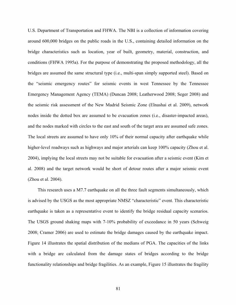
4.1 NETWORK FLOW CAPACITY-BASED NBSR........................................................................ 60 4.1.1 Mathematical Framework ............................................................................................. 61 4.1.2 Monte Carlo Sampling of Bridge Residual Capacity Scenarios ................................... 64 4.1.3 Optimization Models..................................................................................................... 67 4.1.4 Effectiveness Measurement and Project Selection........................................................ 71 4.1.5 Convergence Tests ........................................................................................................ 73 4.1.6 Sensitivity to Ground Motion Correlation .................................................................... 76 4.1.7 Numerical Case Study: the Memphis Road Network ................................................... 80

vii

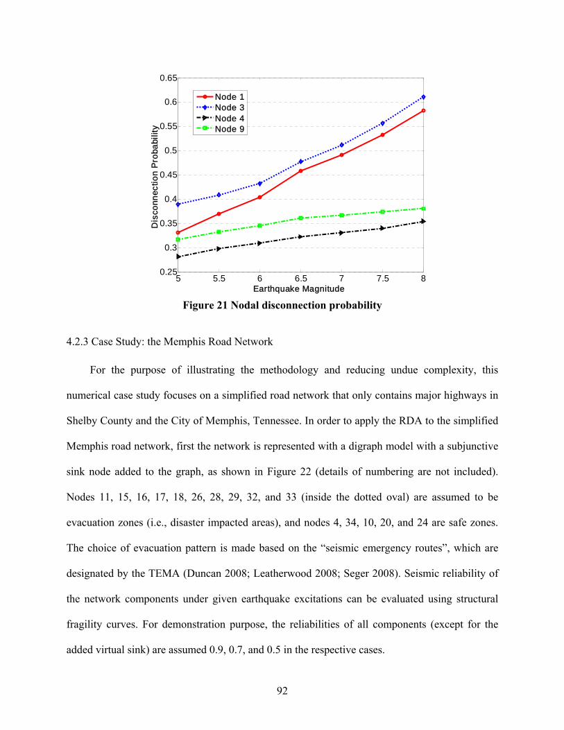
4.1.8 Discussion ..................................................................................................................... 87 4.2 RELIABILITY OF NETWORK REACHABILITY........................................................................ 88 4.2.1 Recursive Decomposition Algorithm for Reachability Reliability ............................... 89 4.2.2 Numerical Example: the Sioux-Falls Road Network.................................................... 90 4.2.3 Case Study: the Memphis Road Network ..................................................................... 92 4.2.4 Results and Discussion.................................................................................................. 93 4.3 SUMMARY.......................................................................................................................... 95

CHAPTER V MODELING THE POST-EARTHQUAKE TRAVEL DEMAND.............. 97

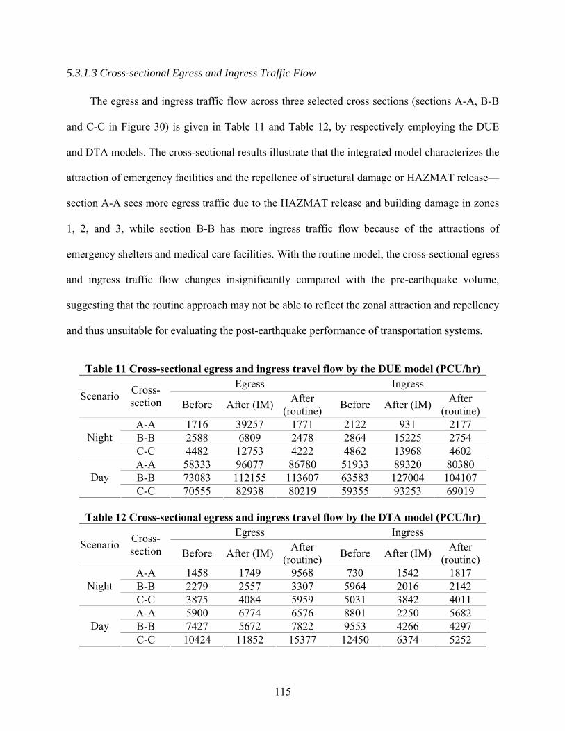
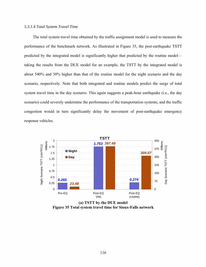
5.1 INTRODUCTION................................................................................................................... 97 5.2 METHODOLOGY FOR TRAVEL DEMAND MODELING........................................................... 98 5.2.1 Scenarios and Major Assumptions................................................................................ 98 5.2.2 Major Modeling Steps................................................................................................. 102 5.3 CASE STUDIES.................................................................................................................. 107 5.3.1 Sioux-Falls Road Network .......................................................................................... 107 5.3.2 Transportation Network of St. Louis MPO................................................................. 117 5.4. SUMMARY....................................................................................................................... 129

CHAPTER VI CONCLUSIONS AND FUTURE RESEARCH......................................... 130

6.1 CONCLUSIONS .................................................................................................................. 130 6.2 FUTURE RESEARCH .......................................................................................................... 133

REFERENCES.......................................................................................................................... 136

APPENDIX A EFFECTIVENESS BASED ON REDUCED REPAIR COST.................. 153

APPENDIX B VERIFICATION OF THE RECURSIVE DECOMPOSITION ALGORITHM........................................................................................................................... 154

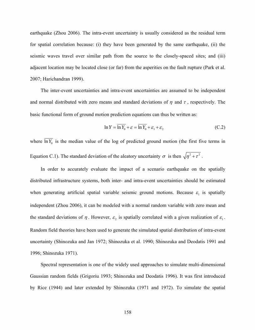
APPENDIX C MODELING UNCERTAINTY AND CORRELATION OF GROUND MOTION ................................................................................................................................... 156

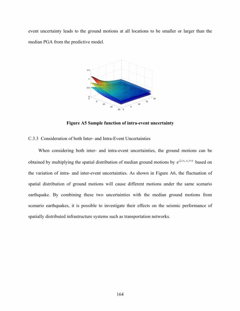
C.1 SIMULATION OF SPATIALLY VARIABLE GROUND MOTIONS ............................................ 156 C.2 PROCEDURES ................................................................................................................... 157 C.3 NUMERICAL EXAMPLE .................................................................................................... 160 C.3.1 Intra-Event Uncertainty ............................................................................................. 160 C.3.2 Inter-Event Uncertainty ............................................................................................. 163 C.3.3 Consideration of both Inter- and Intra-Event Uncertainties ...................................... 164

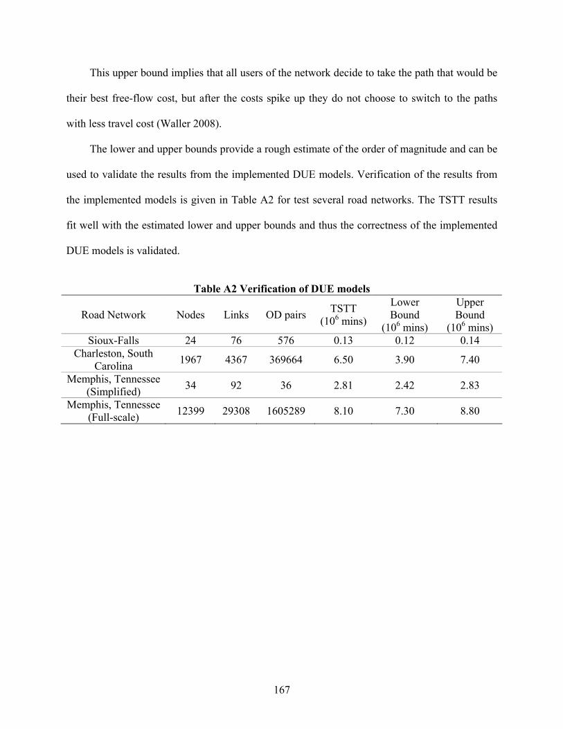
APPENDIX D VERIFICATION OF THE DUE MODELS ............................................... 166

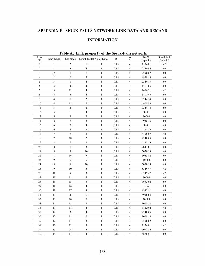
APPENDIX E SIOUX-FALLS NETWORK LINK DATA AND DEMAND INFORMATION....................................................................................................................... 168

viii

LIST OF FIGURES

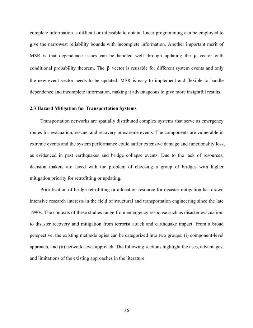
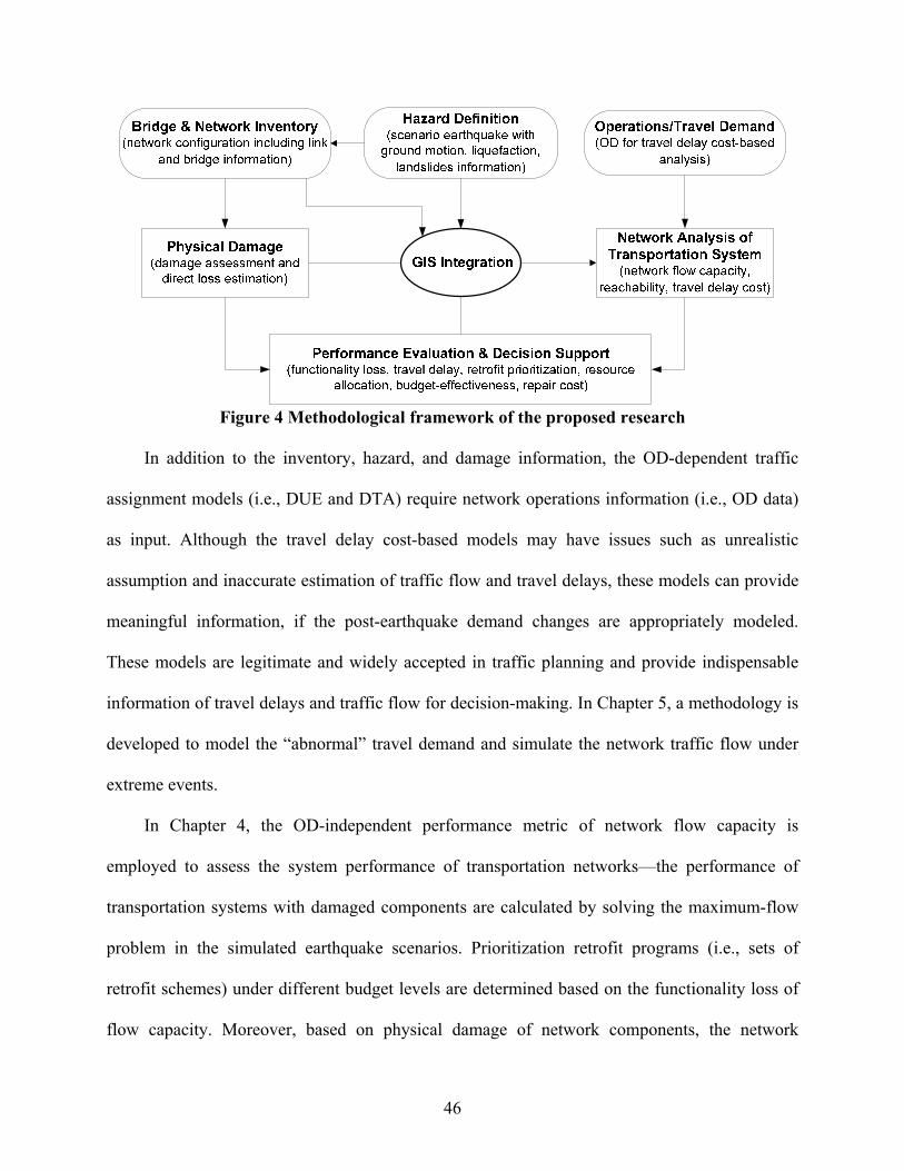
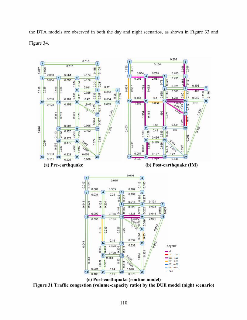
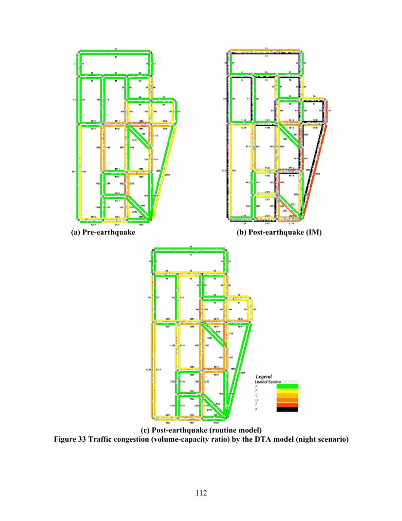
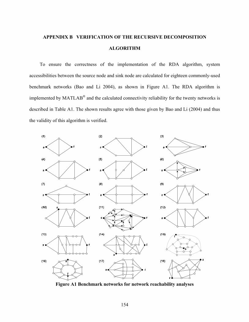
Figure 1 Depiction of structural fragility curves .......................................................................... 10 Figure 2 Travel demands in static and dynamic traffic assignment models ................................. 18 Figure 3 Procedures of the NBSR Approach (Kim et al. 2008) ................................................... 41 Figure 4 Methodological framework of the proposed research.................................................... 46 Figure 5 NMSZ zone structure ..................................................................................................... 49 Figure 6 PGA map of a M7.7 earthquake on all three New Madrid fault segments (g)............... 50 Figure 7 Computing exceedance probabilities for damage states................................................. 52 Figure 8 Methodological framework of network flow capacity-based NBSR ............................. 64 Figure 9 Sioux-Falls network for convergence test ...................................................................... 74 Figure 10 Convergence test of Monte Carlo sampling for network flow capacity....................... 76 Figure 11 Convergence test of network flow capacity ................................................................. 76 Figure 12 NGA hazard map (M8.0) and the Sioux-Falls road network ....................................... 78 Figure 13 Road network in the Memphis metropolitan area, Tennessee...................................... 82 Figure 14 Seismic hazard map for Memphis MPO (the M7.7 NMSZ earthquake scenario) ....... 83 Figure 15 Fragility curves of multi-span simply supported (MSSS) steel bridges....................... 83 Figure 16 Spatial distribution of bridge retrofit program under $1 million budget...................... 86 Figure 17 Budget-effectiveness curves......................................................................................... 87 Figure 18 Illustration of the recursive decomposition algorithm ................................................. 90 Figure 19 Sioux-Falls network for network reachability.............................................................. 91 Figure 20 Probability of disconnection (node 1) .......................................................................... 91 Figure 21 Nodal disconnection probability .................................................................................. 92 Figure 22 Simplified Memphis road network with the subjunctive sink...................................... 93 Figure 23 Reachability reliabilities of network nodes .................................................................. 94 Figure 24 Reliability of reachability to safe zones (case II) ......................................................... 94 Figure 25 Classification of zone types........................................................................................ 101 Figure 26 Illustration of TAZ types............................................................................................ 101 Figure 27 Methodological framework for demand modeling and performance assessment ...... 102 Figure 28 Flowchart of trip generation ....................................................................................... 103 Figure 29 Structural fragility curves for the estimation of damaged buildings .......................... 105 Figure 30 Sioux-Falls road network with evacuation and safe zones......................................... 108 Figure 31 Traffic congestion (volume-capacity ratio) by the DUE model (night scenario)....... 110 Figure 32 Traffic congestion (volume-capacity ratio) by the DUE model (day scenario) ......... 111 Figure 33 Traffic congestion (volume-capacity ratio) by the DTA model (night scenario)....... 112 Figure 34 Traffic congestion (volume-capacity ratio) by the DTA model (day scenario) ......... 113 Figure 35 Total system travel time for Sioux-Falls network ...................................................... 116 Figure 36 Transportation network of St. Louis MPO................................................................. 119 Figure 37 St. Louis MPO PGA map and bridge functionality (day 0) ....................................... 119 Figure 38 Demand generation for St. Louis MPO region........................................................... 120 Figure 39 Traffic congestion of St. Louis MPO network (day scenario) ................................... 124 Figure 40 Traffic congestion of St. Louis MPO network (night scenario)................................. 125 Figure 41 Link traffic flow on major Mississippi River crossing bridges.................................. 126 Figure 42 TSTT for the St. Louis MPO road network................................................................ 128 Figure A1 Benchmark networks for network reachability analyses........................................... 154

ix

Figure A2 Plots of PSD and autocorrelation functions............................................................... 161 Figure A3 Sample functions of inter-event uncertainty (spatial correlation) ............................. 162 Figure A4 Ground motion with intra-event uncertainty (spatial correlation)............................. 163 Figure A5 Sample function of intra-event uncertainty ............................................................... 164 Figure A6 With both intra- and inter-event uncertainties........................................................... 165

x

LIST OF TABLES

Table 1 Fragility parameters for MSC steel bridge (Padgett 2007).............................................. 50 Table 2 Bridge damage-functionality relationship (Padgett and DesRoches 2007) ..................... 53 Table 3 Bridge information for convergence test ......................................................................... 74 Table 4 Post-earthquake network flow capacity........................................................................... 75 Table 5 Effects of ground motion uncertainty and correlation on system performance............... 78 Table 6 Top 20 bridges with highest effectiveness-cost ratios..................................................... 84 Table 7 Network reachability with convergence criteria of 0.001 ............................................... 93 Table 8 Characteristics of zonal traffic generation..................................................................... 101 Table 9 Link traffic flow by the DUE model (PCU/hr).............................................................. 114 Table 10 Link traffic flow by the DTA model (PCU/hr)............................................................ 114 Table 11 Cross-sectional egress and ingress travel flow by the DUE model (PCU/hr) ............. 115 Table 12 Cross-sectional egress and ingress travel flow by the DTA model (PCU/hr) ............. 115 Table 13 St. Louis MPO major river crossing bridges ............................................................... 126 Table 14 Cross-Mississippi River traffic flow............................................................................ 128 Table A1 System connectivity reliability verification for benchmark networks........................ 155 Table A2 Verification of DUE models ....................................................................................... 167 Table A3 Link property of the Sioux-Falls network................................................................... 168 Table A4 Origin-destination matrix for Sioux-Falls network (night scenario) .......................... 170 Table A5 Origin-destination matrix for Sioux-Falls network (day scenario)............................. 170

1

CHAPTER I INTRODUCTION

1.1 Background

Transportation systems, together with energy, water, and telecommunication networks are

the major civil infrastructure systems providing critical backbones of modern societies (Duke

1981). Transportation systems also serve as escape routes for survivors of disasters and provide

an emergency transport network for rescue workers, construction repair teams, and disaster relief

(Earthquake Engineering Research Institute [EERI] 1986). These infrastructure systems are not

only continuously deteriorating over the course of service, but also particularly vulnerable to

seismic hazards. For example, more than 26% of the bridges in the U.S. are either structurally

deficient or functionally obsolete, requiring a $17 billion annual investment to substantially

improve their deteriorating conditions (American Society of Civil Engineers [ASCE] 2009).

The physical damage and functionality loss of the transportation infrastructure systems not

only hinder societal and commercial activities, but also impair post-disaster response and

recovery (Chang and Nojima 1998; Basőz and Kiremidjian 1996; Nojima 1998), resulting in

substantial socio-economic losses (Eguchi et al. 1998; Scawthorn et al. 1997; National Research

Council [NRC] 1999). Transportation networks with collapsed bridges could result in severe

system functionality loss and hamper post-disaster emergency response. For example, emergency

rescuers will not be able to get access to the impacted area if transportation infrastructures

collapse due to earthquake or landslide, as evidenced by the recent devastating earthquakes. It is

crucial that transportation networks retain their traffic carrying capacities after a disastrous

earthquake, so that the population at risk can evacuate efficiently to safe zones and emergency

relief resource be dispatched to the impacted area timely.

2

1.2 Challenges and Issues

Retrofitting the existing bridges of transportation infrastructure systems has been proved a

very effective and relatively economical way to enhance the performance of transportation

systems and mitigate the potential catastrophic losses (Chang et al. 2000; Shinozuka et al. 2003;

Zhou et al. 2004; Kim et al. 2008). However, it is neither practical nor economical to invest very

substantial resources to retrofit all existing bridges. Hence, it is vital to prioritize the bridges for

seismic retrofit with an optimal strategy under the funding and aging challenges (ASCE 2009;

Basőz and Kiremidjian 1996).

Government at all levels has attempted to reduce vulnerability and limit casualties, property

damage, and socio-economic disruption with pre-impact adjustments such as hazard mitigation,

emergency preparedness, and insurances (Lindell and Perry 2000). Of the four stages of

emergency management (i.e., mitigation, preparedness, response, and recovery), mitigation is the

advance action taken to reduce or eliminate the long-term risk to human life and property from

extreme events (Godschalk et al. 1999; Lindell et al. 2006). Decision makers (e.g., the state

Departments of Transportation in the United States, which are usually responsible for the

management, inspection, and maintenance of transportation infrastructures) need to decide how

to strategically allocate the limited mitigation resources to retrofit projects.

Developing such optimal retrofit programs is a challenging problem, as transportation

networks are often large systems with thousands of bridges. In addition, the lack of transparent

performance measures of transportation infrastructure systems inhibits effective reinvestment

decision-making for infrastructures (NRC 1995). Past experience also suggests that the bridge

reinvestment decisions made solely based on the lowest costs or relative importance measures

3

could yield unsatisfactory results (Patidar et al. 2007). Furthermore, stochastic bridge damages

result in the uncertainties in network configuration, making the problem more difficult.

In addition to the seismic mitigation measures that focus on retrofitting transportation

infrastructure, it is essential to understand and model travel demand in emergency situations

when considering measures to secure traffic functions immediately after earthquake and restore

the performance of the transportation systems (Masuya 1998). Under emergency conditions such

as damaging earthquakes, traffic patterns differ significantly from “normal” traffic conditions

due to the changes of post-earthquake travel demand and deteriorated network capacities (Shen

et al. 2009).

Estimation of travel demand is the first step in the traffic modeling but yet the part that has

received the least attention (Wilmot and Mei 2004). As noted by Ziliaskpopoulos and Peeta

(2002), the most challenging obstacle to overcome, before deploying traffic modeling for

planning applications, is to estimate and predict accurate origin-destination demand. The

emergency traffic relies on the operational ability of the transportation infrastructure, and largely

on the response of the evacuating public (Moriarty et al. 2007). Various factors influence public

response, including time of day and day of year, household location and structural characteristics,

gender and age, disaster-specific threat factor, perception of risk, information source and type,

provision of evacuation transportation assistance, local authority action, presence of children or

disability in the household, etc. (Lindell et al. 2005; Baker 1991; Stern and Sinuany-Stern 1989).

The manner in which these factors are addressed has direct effect on the pattern of travel demand.

Approximation of post-earthquake traffic pattern and its recovery over time is complicated

(Zhou 2006) due to too many socio-economic uncertainty aspects (Fan 2006). Post-earthquake

change of traffic demand is partially related to the evacuation of residential and other critical

4

facilities due to excessive seismic damage. Although post-earthquake travel demand contains

emergency operations (e.g., evacuation) that are common in other types of hazards, post-

earthquake traffic is unique in that, among other reasons, the impact is a “no-notice” event; and

after the occurrence, it is less urgent for people to leave. In addition, most of the people in the

impact area will be either trapped in the rubble or trying to extricate those in the rubble. Finally,

many streets in the most heavily impacted area will be blocked by debris, impeding evacuation

(Lindell 2009). Therefore, it is uncommon for governments to declare an earthquake

evacuation—the post-earthquake traffic is usually not considered as an evacuation scenario, but

the change of travel pattern with individuals seeking medical assistance, temporary shelters, etc.

1.3 Objectives and Expected Impact of Research

This brief introduction shows the challenges and issues to model and evaluate the

performance of transportation infrastructure systems under the context of extreme events such as

earthquakes. The objective of this research, focusing on strategic disaster management for

critical civil infrastructures with specific emphasis on transportation networks, is two-fold.

The first objective is to extend the infrastructure evaluation framework of the Mid-America

Earthquake (MAE) Center by providing a systematic methodology to model the performance of

transportation systems under extreme events. The second objective is to generate sound

strategies of seismic mitigation and management for transportation networks to reduce the

likelihood and consequences of extreme events. To achieve the objectives, the specific research

tasks are given as follows:

Review existing methodologies of seismic assessment and modeling of

transportation systems that can be used to improve infrastructure resilience to

disasters and sustainability;

5

Formulate an efficient network-based optimization approach to evaluate the

effectiveness of seismic retrofit projects in terms of preserving post-disaster

evacuation flows;

Develop an integrated transportation simulation model considering the change of

traffic pattern after a damaging earthquake;

Evaluate the reachability reliability of transportation systems (e.g., the accessibility

to critical facilities such as hospitals and shelters using transportation network) in

disaster impacted regions to provide decision support for emergency management;

Demonstrate the proposed methodologies with real-world regional transportation

networks in the Central United States, and assess the applicability and limitations of

these methodologies.

The distinct features of the proposed research are its introduction of the origin-destination

(OD)-independent performance metrics and efficient optimization problem formulation, its

accounting for post-earthquake travel demand changes, and its inclusion of assessment of

reachability reliability of transportation systems.

The study has important academic contribution and implications in disaster response and

mitigation for transportation systems under extreme events. With the proposed methodology, we

are able to prepare strategic mitigation plans for transportation infrastructure systems, and to

model post-earthquake performance of transportation systems. The findings are beneficial for

government agencies and emergency managers to evaluate the performance of transportation

systems and estimate losses induced from damaged bridges or road closures, to improve the

systems’ disaster resilience under economic constraints, and to evaluate the contingency plans

for transportation management.

6

1.4 Scope

This study limits its scope to road networks subject to earthquake hazards. Because bridges

are the most vulnerable components to seismic hazards in a road network (Central U.S.

Earthquake Consortium [CUSEC] 2000; Kiremidjian et al. 2007), this study is limited to

mitigating the vulnerability of road systems through retrofitting bridges. Vulnerability of the

components of road networks other than bridges is out of the scope of this study.

Airports and ports are not included since such transportation facilities are usually not

considered as part of facilities for emergency response purposes. Due to the fact that the railways

in the United States are privately owned and the data is usually not open to the public, railways

are not included due to the unavailability of network data. Tunnels are also not included in this

study, because they have been relatively free of damage during earthquake (EERI 1986).

However, the proposed model can be easily extended without changing the framework to

incorporate the damage of other network components (e.g., roadway segments).

Furthermore, the scope of emergency response such as evacuation is limited to short-term

time frame and only steady-state traffic flow is considered; i.e., the evacuation zones are

assumed to have sufficient demand during the post-earthquake evacuation process, and the flows

from different evacuation zones can be evacuated to any safe zones.

Lastly, although the transportation systems are evident in all models of travel, public transit,

bicycle, and pedestrian modes of travel are not considered since these travel modes are not

dominate for emergency response.

1.5 Organization of Dissertation

The dissertation is divided into six chapters. After this brief introduction, Chapter 2 reviews

the state of the art of earthquake risk assessment of transportation networks. Chapter 3 presents

7

the proposed methodological framework for the network-based performance modeling research.

In Chapter 4, the proposed OD-independent approaches are formulated and demonstrated by

numerical case studies, including the Memphis metropolitan transportation network. Chapter 5

discusses the OD-dependent performance assessment methodology, in which an integrated post-

earthquake demand modeling approach is presented and illustrated with the transportation

network in the greater St. Louis metropolitan area. Conclusions and recommendations for future

research are given in Chapter 6.

8

CHAPTER II LITERATURE REVIEW

The need to protect critical transportation networks against natural disasters has stimulated

intensive research activities in the fields of structural and transportation engineering since the

late 1990s. Seismic risk assessment and decision-making of spatially distributed transportation

systems are particularly challenging because it requires the modeling and assessment of system

performance at network-level as well as the component performance of transportation

infrastructures. This entails the characterization of physical damage of network components and

system response to any given earthquake events.

This chapter presents a review of prior research in risk assessment and modeling

methodologies for transportation systems. The relevant theories and empirical studies are

grouped into three broad categories: (i) the assessment of transportation infrastructure systems at

component-level, (ii) the network-level performance modeling and evaluation of transportation

systems, and (iii) the emergency management and seismic hazard mitigation for transportation

systems. The review of each category contains a discussion of the contributions as well as

limitations found in previous works.

2.1 Seismic Risk Assessment of Infrastructure Components

In emergency management community, risk is a commonly used notion and is essentially

the product of hazard and vulnerability (Alexander 2002). Hazard is the danger or threat of

occurrence of a physical impact under extreme events such as natural and man-made disasters.

Earthquakes are one of the major threats to transportation infrastructures. Broadly defined as the

potential for loss, vulnerability is an essential concept in hazards research and critical in

developing hazard mitigation strategies (Cutter 1996). For example, vulnerability assessments

are used to determine the potential damage and loss of life from extreme natural disasters under

9

the framework of the United Nation’s International Decade of Natural Disaster Reduction

(IDNDR). Seismic vulnerabilities of infrastructure systems, especially the transportation systems

have become an increasing concern since the 1971 San Fernando earthquake. In earthquake

engineering, majority of seismic risk assessment (SRA) methodologies are developed on the

basis of seismic design decision analysis (SDDA) by Whiteman et al. (1975). The generic SRA

methodology considers effects of hazard, damage vulnerability, and losses (e.g., economic loss

or travel delay).

2.1.1 Hazard Definition

Defining seismic hazard requires levels of ground motion as well as ground failure

quantified over the region of interest. Using the attenuation relationship is a way to estimate the

ground motions, which are often expressed as peak ground motion parameters (i.e., acceleration,

velocity, and deformation) or peak structural responses (e.g., peak spectral acceleration [PGA],

velocity, and displacement) (Elnashai et al. 2009). Other essential components of hazard

definition include soil amplification, liquefaction, landslide, and surface rupture.

2.1.2 Structural Vulnerability and Functionality

This section describes and groups the component structural vulnerability and functionality

of transportation infrastructure systems. A review of structural vulnerability and functionality is

given in the following subsections.

2.1.2.1 Structural Vulnerability

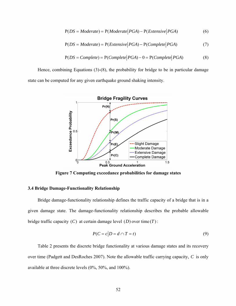
Structural vulnerability dictates the likelihood of a structure (e.g., bridge) being in certain

structural damage states. The probable damage states can be determined once the fragility curves

and hazard information are available. Fragility curves, also know as damage functions or

10

fragility functions, are a key input to seismic risk assessment—bridge fragility curves are

essential for evaluating the expected traffic capacity of bridges and assessing the seismic risk to

the transportation network (Padgett and DesRoches 2007).

Structural fragility is defined as the conditional probability that a certain type of structure

exceeds the prescribed limit state iLS (e.g., moderate structural damage) for a given ground

motion intensity (e.g., taking peak ground acceleration as the intensity measure). Figure 1 depicts

the continuous form of a set of fragility curves and their interpretation at particular ground

motion intensity.

00

0.2

0.4

0.6

0.8

1

Intensity Measure (IM)

Ex

ceed

ance

Pro

bab

ilit

y

Bridge Fragility Curves

Figure 1 Depiction of structural fragility curves

Fragility curves can be developed in several ways. Depending on the development data

sources, fragility curves can be divided into four categories, namely judgmental, empirical,

analytical, and hybrid fragility curves (Rossetto and Elnashai 2003).

Judgmental or expert-based fragility curves are those developed from expert

opinions such as the damage curves given in the ATC-25 report (ATC 1991). The

Applied Technology Council (ATC) conducted a survey to collect expert opinions

x

P(LS1 | IM=x)

P(LS2 | IM=x)

Limit State 1 (LS1)

Limit State 2 (LS2)

11

for estimation of structural damage from earthquakes. The survey results were

represented in a damage probability matrix that describes probabilities of a facility

being in a specific damage state for different level of ground shaking using the

Modified Mercalli Intensity (MMI) scale. Based on the damage probability matrix,

damage curves were developed in the ATC-25 report. However, only five bridge

experts responded and offered their opinion on bridge damages. These judgmental

fragility curves from a small sample-based survey are usually sensitive to systematic

sampling errors and prone to bias (Lindell and Perry 2000; Harrald et al. 1994).

Fragility curves can also be developed based on observations of empirical structural

damage data from past earthquakes (Basőz et al. 1999; Basőz and Kiremidjian 1996;

Yamazaki et al. 1999; Shinozuka et al. 2003). For example, empirical fragility

curves for bridge with and without retrofit were developed based on the field

inspection data collected after the 1994 Northridge earthquake (Shinozuka et al.

2003). The major limitation of empirical fragility curves is the lack of sufficient

empirical data for various types of bridges and damage levels.

In absence of adequate empirical data in the Central United States, analytical

fragility curves are developed based on the evaluation of structural response.

Various approaches have been utilized to develop bridge fragility curves. For

example, elastic spectral method (Jernigan and Hwang 2002) and capacity spectrum

method (Dutta 1999; Mander and Basőz 1999; Federal Emergency Management

Agency [FEMA] 2006; Werner et al. 2006) were used to develop analytical bridge

fragility curves. The analytical fragility curves developed based on non-linear time

history analysis are the most reliable (Shinozuka et al. 2000) and thus have been

12

widely adopted in recent research (Mackie and Stojadinovic 2004; Choi et al. 2004;

Elnashai et al. 2004; Nielson 2005). The applications of the analytical models are

often limited to the most critical components of infrastructure systems (i.e., bridges

in transportation systems) because of their requirements for larger information and

computationally expensive analysis (Eguchi 1984).

Hybrid fragility curves combine data from various sources and compensate for the

scarcity of observational data, subjectivity of judgmental data, and modeling

deficiencies of analytical procedures (Jeong and Elnashai 2007).

With structural fragility curves, the damage probabilities of the components in

transportation infrastructure systems at a particular ground shaking intensity can be obtained.

The post-earthquake traffic carrying capacity of a component of transportation network (e.g.,

bridge) will be time-dependent in accordance to the structural damage and restoration of the

component, as defined by the damage-functionality relationship.

2.1.2.2 Damage-Functionality Relationship

The damage-functionality relationship defines the residual traffic capacity of a component

for a particular damage state. In other words, the damage-functionality relationship maps the

structural damage states to the reduced traffic throughput capacities due to bridge collapse and

lane or road closure, etc. Once the functionalities of components in the network are obtained, the

time-dependent system functionality that corresponds to the level of serviceability or traffic

carrying capacity can be determined.

Similar to the approaches used for developing fragility curves, there are three ways (i.e.,

empirical, analytical, and expert opinion-based) to develop the damage-functionality

relationships.

13

The first category of damage-functionality relationship is based on empirical data.

Observations of repair and restoration and corresponding structural damage from past events are

used to develop the relationship. This empirical approach, as indicated previously, requires

sufficient field observations for various types of structures from past earthquakes. Though this

empirical approach could be effective in regions with adequate observation data, it would be

difficult for regions with little seismic data, e.g., the Central United States.

In addition to the empirical approach, bridge damage-functionality relationship can be

developed analytically by using statistics of structural damage repair and restoration for the

regions with adequate observation data (e.g., California). Mackie (2004) investigated analytical

damage-functionality relationship for typical bridge types in California, in which the

functionality of a bridge was measured by its load carrying capacity. This approach, however, is

not representative because it does not reflect the repair or road closure decisions.

Expert opinion-based approach has been widely employed because it is easy to implement

and effective to capture the subjective nature of bridge functionality that is based on closure and

repair decisions. This approach was used in the ATC-13 (ATC 1985) to evaluate the loss of

functionality and estimate the restoration time for lifeline facilities including transportation

infrastructures. To collect the responses from professionals, a survey questionnaire was

administered to query the participants about the time elapsed before restoring 30%, 60% and

100% functionality at a given bridge damage state. Though only four participants responded to

the bridge survey, these results were later used in HAZUS to establish discrete and continuous

restoration curves (FEMA 2006). Targeting the continuous multi-span concrete bridges in the

Mid-America region, Hwang et al. (2000) conducted a survey to collect expert opinions on

stepwise restoration curves, in which only nine responses were received. More recently, Padgett

14

and DesRoches (2007) performed a web-based survey to collect expert opinions from

experienced staffs in the departments of bridge engineering maintenance and operations of the

Central and Southeastern United States (CSUS). About 75% experts responded to the survey and

the damage-functionality relationship was obtained for the CSUS bridges based on 28 samples.

The drawback of these expert-based relationships is that they are subjective and biased (Lindell

and Perry 2000; Harrald et al. 1994). In addition, the discrete relationships are limited due to the

stepwise function form with the assumption of discrete levels traffic carrying capacity.

2.2 Performance Modeling and Evaluation of Transportation Systems

The need to protect critical transportation infrastructures from extreme events has attracted

increasing research focus for the past twenty years. The contexts of these studies range from

emergency response and disaster evacuation (Jha and Behruz 2004) to disaster recovery and

mitigation (Murray-Tuite and Mahmassani 2004; Basőz and Kiremidjian 1996; Kim et al. 2008;

Liu et al. 2009). In every context, a system performance metric is needed to evaluate the

performance or serviceability of a road network and compare the effectiveness resulted from

various intervention or mitigation projects. Such system metrics for transportation networks can

be divided into three broad categories: (i) travel delay cost, (ii) network flow capacity, and (iii)

reachability (or connectivity).

The first category of metrics (i.e., travel delay cost) depends upon origin-destination (OD)

demand that describes number of vehicle (or person) trips between locations (i.e., origins and

destinations) in the road network; while the latter two categories are OD-independent. OD

demand reflects number of households, income distribution, vehicle ownership, employment

statistics, zoning, and retail-activities. OD demand can be obtained either from surveys and

automatic vehicle identification data, or by mathematical modeling.

15

2.2.1 Travel Delay Cost

Travel delay cost metrics have been widely used in assessing the seismic risk of

transportation systems (Kiremidjian et al. 2007; Nojima and Sugito 2000; Kim et al. 2008). The

travel delay cost metrics can be given by modeling traffic flow distribution and travel time (i.e.,

travel costs) over road networks in the traffic assignment step of the conventional four-step

transportation demand forecasting process (Weiner 1987).

Traffic assignment methods (static or dynamic, user equilibrium or system optimal) have

been one of the most widely used approaches to model traffic flow over road networks since the

first mathematical formulation of static traffic assignment problem was proposed by Beckmann

and colleagues (1956). Traffic assignment models require detailed OD demand and traveler

routing rules as the input. Based on the assumptions on traffic demand and link cost, traffic

assignment models can be grouped into two broad categories: static and dynamic assignment

models.

2.2.1.1 Static Traffic Assignment Models

A static traffic assignment model assumes the model parameters (e.g., traffic demand and

travel cost) do not vary over time. The static models give steady state traffic flow in user

(traveler) equilibrium (UE), in which no traveler in the network can unilaterally change routes

and improve his or her travel time thereby (Wardrop 1952; Sheffi 1985).

Based on the assumptions on the behavior of drivers in their route choices, static traffic

assignment models can be further categorized into two groups: (i) deterministic user equilibrium

(DUE) model, and (ii) stochastic user equilibrium (SUE) model.

The DUE model assumes the driver always choose the shortest path, while the driver’s

route choice is stochastically determined in the SUE model. The assumption of DUE model on

16

driver’s route choice is reasonable in urban road networks since the driver tends to minimize his

or her individual travel time. Therefore, it has been widely used to study the driving behavior in

urban area (Sheffi 1985). SUE assumes the driver chooses his or her route based on individual

preference, which can be measured with the stochastically generated utility or attractiveness. The

SUE model is especially useful for traffic planning in rural areas where traffic is less congested

compared with urban areas, and where not all drivers choose the shortest paths (Sheffi 1985;

Taplin 1999). Additionally, stochastic models can be employed to simulate optimal egress

problem during an emergency such as a fire or earthquake by characterizing the mixing and

confluence of exiting user streams, bottlenecks, slowdown due to hazard prorogation, and

blocking (Talebi and Smith 1985).

Static assignment model provides a fairly good and efficient prediction of the average travel

time and therefore has been widely accepted and employed by many transportation agencies and

practitioners (Kim et al. 2008). In a seismic risk study for a Japanese transportation network,

Nojima and Sugito (2000) evaluated its post-earthquake functional performance based on the

travel costs, which were simulated by a static traffic assignment model. Kim et al. (2008)

evaluated the seismic impact on the road network in Charleston, South Carolina with the static

traffic assignment model (DUE), in which the network performance was measured by the total

system travel time. Viswanath and Peeta (2003) also employed the traveling (routing) cost of OD

pairs as the performance metric to identify critical routes for earthquake response with a multi-

commodity maximal covering network design problem (MCNDP) formulation. In a recent study

by Liu et al. (2009), travel delay cost is taken as one of two effectiveness metrics for measuring

the benefit of bridge retrofit.

17

Although the UE model with inelastic demands (i.e., fixed OD trips) is adequate to model

the region-wide traffic flow (Werner et al. 2006) under normal conditions, its unrealistic static

assumption of the traffic information and drivers’ behavior (Ran and Boyce 1996) make it

impossible to account for dynamics of travel demand and traffic congestion after extreme events.

For example, the model cannot provide adequate estimate of traffic along specific highway links.

As indicated in a validation experiment of traffic flow after the Northridge Earthquake (Werner

et al. 2006), the fixed-demand UE model overestimated the travel time (per trip) ten times the

observed travel time from local traffic reports on some highway segments (i.e., near bridge

collapse at I-10/La Cienega, SR-119/Gothic, and I-5/SR-14) (Caltrans 1995).

2.2.1.2 Dynamic Traffic Assignment Models

In addition to static traffic assignment models, the travel delay cost performance metrics

have also been employed in dynamic traffic assignment (DTA) models to compute the average

travel time or clearance time under extreme events.

DTA models provide an alternative way to address the unrealistic issues with the static

assignment models. Instead of assuming static traffic demand, the DTA models take into account

the fluctuation of road traffic by introducing time-dependent traffic flow and route choices. The

differences of travel demand assumption between static and dynamic assignment models are

illustrated in Figure 2.

18

(a) Static models (b) Dynamic models

Figure 2 Travel demands in static and dynamic traffic assignment models

Since the concept of DTA was first introduced by Yagar (1971), extensive research has

contributed to the theories and applications of dynamic traffic simulation. In a broad perspective,

the DTA models can be divided into two major broad categories: (i) analytical DTA models and

(ii) simulation-based DTA models. The analytical models can be further classified into three

methodological groups: mathematical programming, optimal control, and variational inequality

(VI).

Analytical dynamic traffic assignment models

The mathematical programming approach originates from the static traffic assignment

formulation (Beckmann et al. 1956). Though substantial research has been conducted in

mathematical programming based DTA (Yagar 1971; Daganzo 1994 and 1995; Janson 1994a

and 1994b; Ziliaskopoulos 2000), this approach has an inherent technical limitation and

sometimes fails to provide a suitable description of traffic interactions and dynamics, such as the

asymmetric nature of travel cost functions and time-dependent interaction of traffic flow and

travel time (Boyce et al. 2001).

The optimal control theory-based DTA model was first formulated by Merchant and

Nemhauser (1978a and 1978b) and later refined by Carey (1986, 1987, and 1992) and Friesz et al.

(1989). Though this formulation employs inflow as the control variable and provides attractive

Tra

vel D

ema

nd

Hours

12:00 AM 12:00 AM6:00 PM12:00 PM6:00 AM

Actual Travel Demand

Daily Variation in Travel Demand

Demand in Dynamic Models

Tra

vel D

ema

nd

Hours

12:00 AM 12:00 AM6:00 PM12:00 PM6:00 AM

Actual Travel Demand

Demand in Static Models

Daily Variation in Travel Demand

19

explicit relationship between exit flow and link flow, it requires (i) the exit flow function be

convex to establish an optimal control model with multiple OD pairs, and (ii) the exit flow rate

be positive to satisfy exit flow function and provide realistic flow propagation. In addition, this

formulation suffers from limitations such as the lack of explicit constraints to ensure first-in-

first-out (FIFO) of traffic propagation on transportation networks and preclude holding of

vehicles at nodes, the lack of a solution procedure for general networks (Peeta and

Ziliaskopoulos 2001).

Compared with mathematical programming and optimal control, VI provides a more

general platform with analytical flexibility and convenience to address various dynamic traffic

assignment problems (Peeta and Ziliaskopoulos 2001; Boyce et al. 2001; Nagurney 1998; Friesz

et al. 1996). Therefore, this approach has gained increasing attention for both static and dynamic

network modeling since it was first introduced by Dafermos (1980) for the static traffic

equilibrium problems. However, VI is computationally intensive, raising issues of computational

tractability for real-time deployment, especially for the path-based VI formulation that requires

complete path enumeration (Peeta and Ziliaskopoulos 2001).

Despite their capacities to describe spatio-temporal interactions and traffic flow propagation

in an abstract mathematical manner, analytical traffic representations that adequately replicate

theoretic time and flow relationship and yield well-behaved formulation of DTA models are

currently unavailable, due to the issues of traffic realism and intractable computational cost

arising in the context of complex transportation networks (Peeta and Ziliaskopoulos 2001; Boyce

et al. 2001).

20

Simulation-based dynamic traffic assignment models

In the context of real-world deployment, simulation-based models have gained greater

acceptability (Yang 1997; Mahmassani 2001). Simulation-based DTA models use traffic

simulators to model the complex dynamics of traffic flow and determine traffic propagation on

the network. Several simulation-based DTA models are available, including the DYNASMART

(Mahmassani and Peeta 1995), the DYNAMIT (Ben-Akiva et al. 1997), and the VISTA

(Ziliaskopoulos and Waller 2000). The key limitations of simulation-based DTA model are that:

(i) it is unable to derive the associated mathematical properties through simulations, and (ii) the

computational burden associated with the use of traffic simulator in a real-world deployment

could be operationally restrictive (Peeta and Ziliaskopoulos 2001).

Thus far, only a handful studies established the link between the travel cost metrics and

disaster management by using dynamic transportation systems modeling, though DTA model has

evolved rapidly and been used in real-time traffic operations, traffic planning and management

practices (i.e., intelligent transportation systems). Such metrics have been used to identify the

most vulnerable road segments (Murray-Tuite and Mahmassani 2004), evaluate the effectiveness

of evacuation strategies during emergency evacuation (Tuydes and Ziliaskopoulos 2006; Jha and

Behruz 2004), or determine the spatial distribution and capacities of hurricane shelters (Anil and

Ozbay 2007).

The travel delay cost metrics are highly dependent on origin-destination demand

information. During the short-term response period of a disaster (usually within the first few

days after the impact), however, the post-disaster traffic behavior and demand (i.e., route choices)

could change dramatically (Theodoulou and Wolshon 2004; Werner et al. 2006). The traffic is

most likely under the central control of the transportation management agencies (TMA) (Murray-

21

Tuite and Mahmassani 2004). For example, post-earthquake travel demand could alter

substantially due to travelers’ reaction to bridge damage, road closures, and congestions—many

travelers are unwilling to endure the travel delay and could eventually forego their trips (Werner

et al. 2006). The difficulties of obtaining realistic traveler route choice behavior, in addition to

the computational challenges associated with traffic simulation on complex networks, make

travel delay cost an unrealistic metric for modeling network behavior during the short-term

emergency response period.

2.2.1.3 Travel Demand Modeling

An alternative approach to address the issue of inelastic trip demand is to introduce more

realistic post-earthquake travel demand models to characterize the changes in traveler’s behavior

and routing choices. The following subsections provide a review of existing travel demand

models under post-earthquake situations and evidences from recent major earthquakes in both

U.S. and Japan.

Travel demand modeling, as part of the conventional four-step urban transportation demand

forecasting process (Weiner 1987), is to establish spatial distribution of travel between traffic

analysis zones (TAZ). In other words, travel demand modeling explains where the trips originate

from and where they go, with what travel modes and routes. Since a survey of actual travel

demand would be either extremely expensive or impossible at all, the travel demand modeling is

mostly carried out with simulation approaches.

Traffic modeling in extreme events was first studied in the 1970s for hurricane evacuation.

The focus was shifted to nuclear power plant evacuation after the 1979 Three Mile Island

accident but was directed back to hurricanes again in the 1990s. Earthquakes-related traffic

modeling has drawn attention lately, especially after the recent tsunamis and earthquakes in Asia.

22

Review of existing travel demand models

Though many simulation packages are available to model traffic under normal conditions

(e.g., CORSIM, VISSIM, and EMM/2), only a handful models have been developed for use in

emergency conditions. These include, but not limited to, the Oak Ridge Evacuation Modeling

System (OREMS), the Dynamic Network Evacuation (DYNEV), Transportation Emergency

Management of Post-Disaster Operations (TEMPO), and the Evacuation Traffic Information

System (ETIS). Other similar evacuation packages include NETVAC (Sheffi et al. 1981),

HURREVAC (USACE 1994), and MASSVAC (Hobeika and Jamei 1985).

OREMS is designed to estimate evacuation time and develop traffic management strategies

under different events or scenarios (Rathi and Solanki 1993; ORNL 2002; Chang 2003). OREMS

can be used to identify evacuation routes and identify bottlenecks as well as to assess the

effectiveness of alternative traffic control and evacuation strategies (Moriarty et al. 2007).

DYNEV was traditionally developed to simulate the evacuation from nuclear power plant, but

later enhanced for modeling hurricane evacuations (Moriarty et al. 2007; Chang 2003; Mei 2002).

ETIS is a transportation simulation tool developed by the U.S. Department of Transportation to

forecast large cross-state traffic volume for hurricane evacuation (Chang 2003; Wolshon et al.

2005; PBS&J 2003).

Both OREMS and DYNEV require similar TAZ-based inputs such as population of

residents, employment/income, and number of vehicles per dwell unit. Users need define

parameters of behavior patterns (participation rate), day of year/time of day, and basic weather

conditions. Gravity models are used in both OREMS and DYNEV during the trip distribution

step. The difference between OREMS and DYNEV is that DYNEV includes mode-split step and

assumes static assignment (Chiu et al. 2005). ETIS requires county-based inputs such as the

23

population of residents/tourists and the destination percentage of evacuees for each county.

Travel demand is manually generated during trip distribution period. Sigmoid curve loading

model (Yazici and Ozbay 2008; Fu 2004) is employed to simulate time-dependent behavioral

response in ETIS.

The staged model (Southworth 1991; Wilmot and Mei 2004; Moriarty et al. 2007) is the

most widely accepted approach to describe the traffic demand modeling under hurricane and

nuclear hazards. The first stage is to estimate travel demand by using the number of at-risk

population and its response to evacuation orders (Wilmot and Mei 2004); then trip distribution

models are employed to generate trip matrix with gravity model or manual assignment. The

second stage, also known as network loading stage (Southworth 1991), is to load the travel

demand to the transportation network with models that simulate the departure time.

Modeling the travel demand and traffic following earthquakes is much more complex than

hurricane or nuclear-related hazards, partially due to the fact that post-earthquake travel demand

is coupled with the deteriorated capacity of post-earthquake transportation infrastructures.

Additionally, public response to earthquake is distinct because prior warning for earthquakes is

usually unavailable or infeasible, which makes the post-earthquake traffic pattern less dependent

on the behavioral response or network loading model.

TEMPO is a decision support system developed during the aftermath of the 1989 Loma

Prieta earthquake, which specifically addresses the transportation needs following a major

earthquake such as emergency vehicles and repair crew routing and traffic diversion (Ardekani

1992b). The post-earthquake demand model used in TEMPO, however, is solely based on the

physical damage of transportation infrastructure (i.e., the closure of roads) and does not consider

the changes of travel behavior after the earthquake impact.

24

It has been noted that the pre-earthquake travel demand was inappropriate for evaluating

the post-earthquake performance of transportation networks (Fan 2006; Shinozuka et al. 2005;

Kiremidjian et al. 2007). The change of post-earthquake travel patterns has been taken into

account when evaluating the performance of transportation systems (Shinozuka et al. 2005;

Kiremidjian et al. 2007). Other related research on long-term travel demand change under

earthquake impact has been conducted with multi-regional input-output models (Ham et al.

2005a and 2005b; Kim et al. 2002).

The approaches and models that reflect short-term post-earthquake travel pattern changes

can be grouped into two broad categories: (i) model trip demand changes by modifying the pre-

earthquake normal OD matrix (Shinozuka et al. 2005; Wakabayashi and Kameda 1992); and (ii)

employ alternative assignment models such as the modified incremental assignment method

(Nojima and Sugito 2000) and the Variable Demand Model (VDM) (Fan 2006; Kiremidjian et al.

2007).

Shinozuka et al. (2005) estimated the post-earthquake demand matrix by modifying the pre-

earthquake origin-destination data. They introduced trip reduction factors by building occupancy

and trip purposes to account for zonal trip activity changes due to building damage from ground

shaking. Then a combined assignment and distribution models were employed to predict post-

earthquake travel delay. However, essential influencing factors such as emergency shelters and

release of hazardous materials (HAZMAT) were not addressed in their study. The reduction

factors are also limited, as they require additional information such as the type of trip purpose

(e.g., home-based work trips or home-based school trips) that may not be available in all traffic

planning organizations.

25

The similar idea of using travel demand modifiers was also employed in some other recent

research to incorporate the changes of travel demand and reduction of road capacities due to

seismic damage. For example, Kim (2009) designed post-earthquake emergency scenarios that

incorporate demand changes due to HAZMAT release and emergency shelters—areas with

HAZMAT release were taken as repellent zones where link capacities are reduced to 1% of their

original values; areas with shelters are taken as attraction zones with an additional 30% demand.

Wakabayashi and Kameda (1992) estimated the post-earthquake OD matrix due to the Bay

Bridge closure after the Loma Prieta earthquake, by linking the link flow data from eight traffic

observation sites and the census population data. The highway system in the San Francisco Bay

Area was simplified into a 23-node network and the gravity model was employed to distribute

the vehicle trips. This approach, however, did not consider the building damage information, nor

did it account for other demand changing factors such as shelters and HAZMAT release.

Another category of approach to modeling post-earthquake trip demand is to reflect the

demand changes with alternative traffic assignment models (Fan 2003; Werner et al. 2006;

Kiremidjian et al. 2007). Nojima and Sugito (2000) proposed the modified incremental

assignment method (MIAM), an alternative assignment model to obtain the post-earthquake OD

matrix. MIAM loads the damaged network with pre-earthquake OD trips and the output OD-

matrix from the modified method is different from the pre-earthquake one because part of the

OD trips may not be satisfied due to physical isolation of centriods, overload, and/or congestions

(Nojima and Sugito 2000). This method, however, can only provide an approximate solution and

generally is not able to find equilibrium solutions (Lu 2006).

In a study to evaluate the earthquake risk to transportation system in the San Francisco Bay

Area, Kiremidjian et al. (2007) defined the user equilibrium with a variable-demand model

26

(VDM) and compared the travel delays resulting from damage to ground shaking with a fixed

demand model (or FDM). The VDM provides a relative reasonable assumption of elastic travel

demand (DfT 2006), e.g., the travel demand decreases as the travel time between OD-pairs

increases because of reduced link capacity; while the fixed demand model assumes the travel

demand is unchanged before and after the earthquake. It was found that: (i) post-event travel

times increase significantly with FDM assumption, and (ii) the travel times remain relatively

unchanged and decrease with VDM assumption. These findings confirm the field observations

after the Northridge Earthquake (Werner et al. 2006). REDARS 2 also employs the VDM model

to account for the post-earthquake travel demand change (Werner et al. 2006).

Though the VDM models are able to represent the post-earthquake changes of travel pattern

to some extent, two major underlying assumptions may limit the application of the VDM models

in California only, because (i) the assumption of reduced network traffic capacity would cut trip

demand (Kiremidjian et al. 2007) and increase travel time may not be true for all OD-pairs, and

(ii) the predicted equilibrium OD-pair travel time may not always fall on the demand curves

(Werner et al. 2006). The VDM analysis by Kiremidjian et al. (2007) assumes that traffic

demand decreases as observed following both the 1989 Loma Prieta and 1995 Northridge

earthquakes (Yee and Leung 1996a and 1996b; Werner et al. 2006). This assumption of

decreased post-earthquake demand is based on the commuters’ behavior in the study region only

and thus the findings are pertain to traffic patterns observed in California. Traffic patterns could

be completely different in other regions or countries—the travel demand significantly increased

following the 1995 Kobe earthquake due to unique rerouting conditions (Kiremidjian et al. 2007).

27

Evidences from recent earthquakes

This section presents the observed changes of traffic patterns following major historic

earthquakes in the United States and Japan, including the 1989 Loma Prieta earthquake, the 1994

Northridge, the 1995 Hanshin-Awaji earthquake, and the 2004 Niigate Ken Chuetsu earthquake.

These two countries are chosen because both countries have well-developed transportation

infrastructures as well as high seismic risks.

Loma Prieta earthquake (U.S.)

Transportation network was the hardest hit infrastructure system in the 1989 Loma Prieta

earthquake ( wM 6.9). The major disruptions of highway service were in San Francisco, Oakland,

and the major bridges between the two cities. The collapse of a section of the Bay Bridge

seriously impacted the Bay Area travel. The cross-bay traffic volumes on other major bridges

increased significantly after the earthquake—post-earthquake traffic volume on the San Rafael

Bridge increased by 79.9% than the pre-earthquake volume (Housner and Thiel 1990). As a

result, approximately 0.3 million commuter traffic (EQE 1989) had to use alternate city surface

streets for nearly three years after the earthquake (Ardekani 1992a). Surface streets in San

Francisco were also struck heavily—the hardest hit Marina District in the City of San Francisco

was evacuated immediately after earthquake and public access was restricted.

Northridge earthquake (U.S.)

Though the 1994 Northridge earthquake ( wM 6.7) is one of the costliest earthquakes in U.S.

history and the ground acceleration was the highest ever instrumentally recorded in an urban

region in North America (SCEC n.d.), damage to the highway structures was not enormous due

to the $1.5 trillion retrofit program in California. The earthquake caused major damage on the

following four freeways and interchanges: Interstate 5 (I-5, the Golden State Freeway), Interstate

28

10 (I-10, the Santa Monica Freeway), State Route 14 (SR-14, the Antelope Valley Freeway), and

State Route 118 (SR-118, the Simi Valley Freeway). Minor damages also occurred at many other

locations, but none of the damage-incurred closures at these locations lasted more than a few

weeks. Most parts of the local street network were not significantly affected by the earthquake.

Among the four significant freeway damage locations, damages at two locations, namely

SR-14/I-5 interchange and I-10 are notable (Boarnet 1996). The damage at SR-14/I-5

interchange that links the residential suburb in Santa Clarita Valley and the City of Los Angeles

left more than 280,000 commuters with little choice but to take detour and endure traffic delays

that were initially greater than an hour during peak periods (Barton-Aschman and Associates

1994; Ardekani 1995).

Except for the first few days after the earthquake, excessive delays were not experienced

and the transportation systems in Los Angeles continued to function throughout the

reconstruction period (Yee and Leung 1996a and 1996b). The area wide traffic volumes

substantially decreased than normal during the first few days following the earthquake. Travel

delays were substantial in the first few days following the earthquake (EQE 1994), although

alternative travel modes (e.g., public transit) were taken (Debban 1995). The travel demand

increased dramatically within in the following week because workers began returning to their

jobs, but still lower than normal. After the first week, although congestion was bad in some

places, excessive congestion was not experienced except for the Santa Cruz area, which was

isolated due to lack of redundancy (Webber 1992; Tsuchida and Wilshusen 1991). During the

first month, most delays were greater than thirty minutes. Many damaged freeways were repaired

within a few months of the Northridge Earthquake. By March of 1994, the travel demand during

the peak hours stabilized throughout the area (Yee and Leung 1996a) and delays on most

29

transportation corridors stabilized at five to twenty minutes (Barton-Aschman and Associates

1994).

Note that the short-term changes in travel pattern were not entirely commuters’ responses to

transportation system disruptions—many people stayed at home for the week following

earthquake (Schmitt 1998). Moreover, because the earthquake occurred very early on the Martin

Luther King Day, a U.S. national holiday, many trips would not have occurred anyway.

Great Hanshin (Kobe) earthquake (Japan)

The 1995 Hanshin-Awaji earthquake ( wM 6.8) in the Osaka-Kobe area had an even greater

impact on the transportation systems compared with the Loma Prieta and Northridge earthquakes

in the U.S. The span collapses of the elevated Osaka-Kobe expressway (Route 3) caused long-

time closure of this major transportation corridor. The travel demand surged following the

earthquake (Kiremidjian et al. 2007). In addition, parallel routes also suffered major damage to

bridges and elevated section of both the Shinkansen and commuter rail lines (Buckle and Cooper

1995).

Niigate-Chuetsu earthquake (Japan)

In the 2004 Niigate Ken Chuetsu earthquake ( wM 6.9), transportation systems such as the

Shinkansen (the Japanese high-speed rail network) and expressways were significantly disrupted,

especially in the Chuetsu region. The overall performance of the transportation systems, however,

was good (Ashford and Kawamata 2006) partially because detour routes contributed to

interregional travel and commodity flow (Tatano and Tsuchiya 2008). Until the 13th day after

the earthquake, freight transit time between Tokyo (Kanto region) and Niigate increased by 25%

and business travel cost by 9%-30%. It took two weeks to reconstruct the damaged expressways

and two months for the Shinkansen to resume operations (Tatano and Tsuchiya 2008).

30

The observed impact on the performance of transportation systems and post-earthquake

travel patterns from the recent U.S. and Japanese earthquakes suggest that, firstly, transportation

infrastructures are especially vulnerable to earthquake impact and many of the disruptions to

transportation systems are due to damages to bridges or viaducts. In addition, transportation

corridors linking suburban residential areas to downtown region, if damaged, are prune to

significant delays. Transportation networks with less redundancy could lead to serious traffic

problem, as observed in the Santa Cruz area in Loma Prieta earthquake. Furthermore, post-

earthquake travel demand is transient, which could change drastically (surge or decrease) during

the first few days or weeks following an earthquake. The travel demand may need a few months

to stabilize—people are willing to travel as the post-earthquake recovery actions are taken (e.g.,

repair or reconstruction of damaged bridges and/or roadways). Finally, post-earthquake travel

patterns are distinct in different regions, as was found in the California and Kobe earthquakes.

2.2.2 Network Flow Capacity

As an alternative to the travel cost-based metrics, network flow capacity (Nojima 1998;

Chen and Tzeng 1999) can be used as a performance metric of transportation networks.

Maximum flow is the largest possible flow between source nodes and sink nodes without

exceeding the capacity of any link in the network (Ahuja et al. 1993).

This metric is an obvious property of the network itself, and is hence independent of the

traveler behavior and OD demand. Compared with the travel delay cost metric, the network flow

capacity metric is employed in a relatively smaller number of studies. Nojima (1998) evaluated

the post-earthquake serviceability of a transportation network, in which the maximum flow

capacity was used to find Birnbaum’s importance measure for the network links. Nojima’s

maximum flow capacity, however, is rather an intermediate measure that was used to find

31

Birnbaum’s probabilistic importance than a system-level performance metric. Feasible flow

capacity, a variation of the maximum flow capacity, was used as one of the measures in a post-

earthquake road network reconstruction-scheduling problem (Chen and Tzeng 1999). The

feasible flow capacity is taken as one of the objectives in the formulated multi-objective

optimization model. Lee et al. (2010) estimated the post-hazard traffic flow capacity of a bridge

transportation network, in which the flow capacity is given by a standard maximum flow

algorithm. In these studies, the network flow capacity-based formulation, however, did not

account for the resource constraints, nor did they include the bridge components in the

transportation systems. Although some research has been done, to the best of our knowledge,

such network capacity metrics are not currently considered in seismic retrofit planning to

improve the emergency flow capacity of a transportation network in immediate population

evacuation scenarios.

2.2.3 Reliability of Network Reachability

Defined as being able to get from one vertex in a digraph to some other vertex in graph

theory, the reliability of network reachability (also know as connectivity reliability) is one of the

most frequently used measures for networked systems. For transportation systems, the

connectivity denotes the reachability of an arbitrary node-pair via at least one path. Connectivity

highly depends on the post-earthquake completeness or connectedness of a transportation

network and hence it is suitable for the case of immediate post-disaster humanitarian aid. The

network systems’ traffic capacities, travel times, and trip lengths, however, are ignored in the

reachability analyses. Instead, the reachability analyses seek only to determine whether, or with

what probability, a path remains operational (or connected) between the given sources and

destinations (Rojahn et al. 1992). If the path (or paths) connects the selected node-pair following

32

an impact, serviceability (or performance) analyses seek additional information on the remaining

or residual capacities that can be found mathematically by convolving component capacities with

infrastructure completeness (Rojahn et al. 1992).

Considerable advances have been made in the field of network connectivity and various

algorithms proposed to analyze the network reliability since the 1970s'. These network reliability

analysis algorithms can be grouped into two broad categories: (i) simulation-based algorithms

(e.g., Monte Carlo simulation), and (ii) analytical algorithms (e.g., the decomposition methods

and binary decision approaches).

2.2.3.1 Simulation-Based Algorithms

Simulation-based algorithm such as Monte Carlo simulation (MCS) is one of the most

widely accepted approaches to evaluate system connectivity. These algorithms do not rely on

analytical models or graphical representation—all information needed to implement simulation is

the component reliabilities and network configuration (e.g., network topology). Because of its

simplicity of implementation, MCS is widely used in many engineering applications when

analytic approaches are not feasible. Though MCS cannot give exact solution and take longer

time to converge, the results are fairly good and close to exact solutions. Therefore, MCS is

widely accepted as an alternative approach to validate the results obtained in other ways.

Employing MCS approach to evaluate the connectivity reliability of a network is

straightforward—first, random numbers following the uniform distribution (0,1)U are generated

to simulate failures of network components; then graph search algorithms (e.g., the breadth-first

search [BFS]) are used to determine the connectivity of node-pair in the network. This process is

repeated for thousands of times or more and the frequencies of connectivity are takes as network

reliability. In general, a mid-size network requires two thousand to ten thousand of simulation

33

runs and a larger network ten thousand to one hundred thousand of runs to converge a stable

reliability estimate (Li 2005).

MCS is easy to implement and can be applied to any size and any types of networks. MCS

has been extensively used to evaluate utility systems’ connectivity. Oppenheim (1977) simulated

seismic damage of water delivery systems and transportation networks with Monte Carlo

simulation-based method. Shinozuka et al. (1981, 1992, 1996, and 2003) employed MCS to

assess seismic reliability of various infrastructure systems, including water delivery networks,

highway networks, and power networks in Tennessee and California.

However, the shortcomings of simulation-based MCS are also obvious. Firstly, the

convergence is not controllable. It could take thousands of simulation runs to get a stable result,

and the number of simulations to achieve convergence is sensitive to component reliability. In

addition, MCS is based on the independence assumption of component failure and thus difficulty

to account for the dependence between infrastructure systems and their components. Furthermore,

MCS is the least economical way to evaluate network reliability and usually take much longer

time than other approaches. Lastly, the results given by MCS are not informative and limited to

the estimation of reliability only.

Although the simulation-based algorithms are easy to implement and are applicable to large

networks, they are computationally inefficient and usually incapable of controlling the accuracy.

In contrast to the simulation-based algorithms, the analytical ones are able to give exact or more

accurate results with less time consumption for small-scale networks. The following section

provides a review of analytical algorithms for network reachability calculation.

34

2.2.3.2 Analytical Algorithms

The fundamental idea of analytical approach for network connectivity is to convert a

complex network to combination of simply networks such as parallel or series systems; and then

system connectivity could be computed by finding the union and intersection of these simply

networks, e.g., a generic substation can be modeled with a series system of macro-components

(Vanzi 1996).

Kroft (1967) first proposed the shortest path-based algorithm to compute the network

connectivity reliability. Panoussis (1974) and Taleb-Agha (1975 and 1977) demonstrated that

general connectivity reliability can be computed by converting complex infrastructure networks

to SSP (series systems in parallel) networks. Aggarwal and Misra (1975) proposed a disjoint

shortest path algorithm. However, these methods are constrained to small networks due to the

complexity of large network systems. Based on the idea of disjoint path searching, researchers

(Dotson and Gobien 1979; Yoo and Deo 1988; Torrieri 1994; He and Li 2001; Li and He 2002)

later improved this algorithm and found it can give exact connectivity for large complex

networks. The full-probability analytic algorithm (Wu and Sha 1998) and the ordered binary

decision diagram (OBDD) algorithm (Kuo et. al 1999) are also able to find exact network

reliability but neither of them is able to handle large networks.

Connectivity between node-pairs can be evaluated based on the network configuration with

graph theory. The connectivity reliability can then be assessed if the reliability information of

network components is available. The recursive decomposition algorithm (RDA) is a method to

evaluate seismic reliability for large infrastructure systems (Li and He 2002). Using the De

Morgan’s rule and disjoint theorem (Aggarwal and Misra 1975; Ahmad 1982; Liao 1982; He and

Li 2001; Li and He 2002), the RDA recursively decomposes the network into sub-graphs until

35

there is no path existed between the source-terminal node-pair in all the sub-graphs. It is

noteworthy that the RDA is not aiming at finding all the disjoint link or cut sets but rather

estimating system reliability or failure probability (Chang and Song 2007). In addition, this

algorithm will face difficulties in finding all the disjoint link/cut sets for large complex networks.

In such cases, the RDA gives an approximate solution with reliability bounds instead by

terminating the decomposition process with a predefined allowable error (e.g., 0.1%).

On the other hand, since complete information is not always available, especially for

complex systems, researchers chose to approximate system reliability with reliability bounds.

Ditlevsen (1979) gave the theoretical bounds for general system reliability problems. However,

the theoretical bounds are often too wide to be of practical uses. Song et al. (2003 and 2006)

obtained much narrower reliability bounds of the reliability of power substation systems by

employing a linear programming approach. Song and Kang (2007) generalized the linear

programming approach and proposed a matrix-based system reliability (MSR) method to account

for dependence and incomplete information. This method takes advantage of matrix-based

language such as MathWorks MATLAB® to compute system reliability directly from two

vectors: the c vector, which is a representation of the combination of mutually exclusive and

collectively exhaustive (MECE) events, and the p vector, describing the corresponding event

probability. This method is efficient and easy to implement by means of “dot-multiplication”

(component-wise multiplication) with MATLAB®. The MSR method has recently been further

developed for evaluating the multi-scale system reliability of lifeline infrastructure systems

(Song and Ok 2010). One of the merits of MSR is that it could give reliability bounds when

complement information is not available. In case of complete information is available, event

vector and probability vector can be constructed to find the system reliability with MSR; when

36

complete information is difficult or infeasible to obtain, linear programming can be employed to

give the narrowest reliability bounds with incomplete information. Another important merit of

MSR is that dependence issues can be handled well through updating the p vector with

conditional probability theorem. The p vector is reusable for different system events and only

the new event vector needs to be updated. MSR is easy to implement and flexible to handle

dependence and incomplete information, making it advantageous to give more insightful results.

2.3 Hazard Mitigation for Transportation Systems

Transportation networks are spatially distributed complex systems that serve as emergency

routes for evacuation, rescue, and recovery in extreme events. The components are vulnerable in

extreme events and the system performance could suffer extensive damage and functionality loss,

as evidenced in past earthquakes and bridge collapse events. Due to the lack of resources,

decision makers are faced with the problem of choosing a group of bridges with higher

mitigation priority for retrofitting or updating.

Prioritization of bridge retrofitting or allocation resource for disaster mitigation has drawn

intensive research interests in the field of structural and transportation engineering since the late

1990s. The contexts of these studies range from emergency response such as disaster evacuation,

to disaster recovery and mitigation from terrorist attack and earthquake impact. From a broad

perspective, the existing methodologies can be categorized into two groups: (i) component-level

approach, and (ii) network-level approach. The following sections highlight the uses, advantages,

and limitations of the existing approaches in the literature.

37

2.3.1 Component-Level Approaches

Component-level approaches are usually well understood by decision makers with different

backgrounds and hence have been used intensively to provide decision-making support on bridge

retrofit or repair project prioritization. Such decisions may be made based on single or multiple

attributes, which could be subjective engineering judgments (e.g., structural appraisal ratings in

the NBI database) or natural attributes (e.g., average daily traffic). A variety of methods has been

employed to obtain prioritization, varying from simple direct ranking method to the analytical

hierarchy process (AHP).

Bana e Costa et al. (2008) developed a multi-criteria additive model to evaluate the

strategic importance of bridges and tunnels in Lisbon, Portugal. The five criteria used as

fundamental points of view are: (i) emergency response, (ii) vulnerability, (iii) public safety, (iv)

interference with other lifelines, and (v) long term economical impacts. The overall strategic

importance values of bridges and tunnels were then aggregated in an additive model with scaling

factors for the five attributes. Kusakabe (2004) employed the AHP approach to perform the

weighting and calculated the overall bridge seismic retrofit priorities based a three-level and

thirty-item hierarchy. In a study that developed retrofit program for the City of Los Angeles,

California, prioritization of the seismic bridge retrofit program was carried out with a weighted

formula based on replacement cost, condition of the bridge, traffic flow, and the year of

construction (Kuprenas et al. 1998). The bridges selected for the program were prioritized based

on a weighted seismic risk value score equation:

0.5 0.2 0.15 0.15S C O T AR F F F F (1)

where SR is the seismic risk (higher risk score indicating higher retrofit priority) , CF is the

replacement cost, OF is the overall rating coming from the City Files of Structures database

38

maintained by the Structural Engineering Division, TF is the equivalent traffic, and AF is the

year of built.

Similar weights-based approaches were employed by ATC (1983), Babei and Hawkins

(1991), and Federal Highway Administration (FHWA) (1995b) by using judgmental weights and

attributes of seismic hazard, structural resistance, fragilities of bridge structural elements (e.g.,

pier, seating, abutment, foundation), and cost of failure, etc. Note that these weights or scaling

factors are all based on engineering judgment and very subjective (FIB 2007). Therefore, these

methods were most useful as a relative measure of prioritization for clearly defined objectives or

goals (e.g., economic cost, travel delay, transportation safety, etc.) and not as an absolute

measure.

In addition, ranking-based approaches have been widely used for retrofit priority. Basőz

and Kiremidjian (1996) proposed a ranking-based bridge retrofit prioritization methodology for

emergency preparedness. The relative importance of a bridge was measured by the ranking of

bridge vulnerability as well as the importance factor accounting for network behavior (e.g.,

network connectivity between a predefined OD-pair). The maximum flow-based Birnbaum’s

probabilistic importance measure was employed to obtain the prioritization in updating seismic

performance of a road network (Nojima 1998). The Birnbaum’s probabilistic importance

measure implies the probabilistic contribution of improving component reliability to that of

system reliability (Henley and Kumamoto 1981). It can be calculated for road segment i as

follows:

( )(1 , ) (0 , )B

i i ii

PI P P

p

p

p p (2)

39

where BiI is the Birnbaum’s importance measure for i -th component, ( )P p is the system

reliability as the function of the component reliability vector 1 2{ , , }np p pp = , (0 , )iP p and

(1 , )iP p are the conditional system reliabilities given that the component (i.e., road segment)

fails or not, respectively.

The level of significance for a network component can also be ranked by the incurred

transport cost or economic loss from the earthquake impact (Sohn et al. 2003). A direct approach

was also proposed by Kim et al. (2008) to select the bridges for retrofit prioritization. This

approach calculated the relative importance of each bridge (i.e., the resultant incremental of total

system travel time by reducing of the post-earthquake traffic capacity of one bridge to 1% of its

original capacity) and then sorted the bridges by descending order of their contributions, on

which the decisions on retrofit prioritization can be made.

These previous studies focused on component-level analyses, dealing the network by

individual or a group of similar components. However, the inter-relationship of bridges in a

common network (i.e., the system behavior of transportation networks) was not taken into

account (Liu and Frangopol 2005). Past experience also suggests that the decisions made solely

based on some ranking index are highly dependent on the procedures used (Small 2000) and

often yield unsatisfactory results (Patidar et al. 2007).

2.3.2 Network-Level Approaches

Although the vital role of bridges in transportation networks has long been recognized, few

research managed to prioritize retrofit projects from a network viewpoint. Since the overarching

goal of bridge retrofit and maintenance is to improve transportation system’s performance and

40

mitigate potential impact from extreme events, network-level approaches represent a significant

advancement.

A variety of mathematical programming formulations has been used for problems of

maintenance planning of transportation infrastructures. Augusti et al. (1994) studied the

allocation of retrofit resource for seismic protection of a highway network using dynamic

programming. The objective is to maximum network connectivity at given seismic intensities

and under a budget constraint.

Since the bridge retrofit prioritization problem is similar to a nondeterministic polynomial-

time hard (NP-hard) discrete network design problem (DNDP), Kim et al. (2008) proposed a

network-based seismic retrofit (NBSR) problem formulation with variable capacity constraints

and budget constraint. To propose an optimal retrofit strategy at various budget levels during the

emergency preparedness planning process, the problem was reformulated into a multi-objective

optimization problem to facilitate decision-making process. The two objectives of NBSR are: (i)

to maximize the network performance, that is, to minimize the expected total system travel time,

and (ii) to minimize the total retrofit cost, respectively. Meta-heuristic methods such as Simple

GA (SGA) and Non-Dominated Sorting Genetic Algorithm (NSGA)-II were utilized to solve the

network design problem (NDP) formulations.

The procedures of the NBSR framework are illustrated in Figure 3. The travel delay cost

metrics were employed to provide essential information on traffic flow changes of and travel

delays that result from particular route closure due to excessive damage to key infrastructure

elements, or from the reduced traffic carrying capacity because of less severe damage (e.g., lane

closure for repair or imposed lower speed limit). The post-event system performance with “as-

41

built” and “retrofitted” bridges was assessed with traffic assignment models and prioritization

recommendations are made based on the assessment of system functionality loss.

Figure 3 Procedures of the NBSR Approach (Kim et al. 2008)

The advantages of this NBSR methodology are the integration of seismic risks, structural

vulnerabilities and functionalities, and network behavior of transportation system for decision-

making. However, the authors recognized that the most critical issue of NBSR is the

computational costs. The simulation time would be unbearable for large networks due to

extensive computational burdens of traffic modeling. For similar reasons, it is impractical to

solving NBSR with theoretically required population size and number of generations to get

optimal solutions in GA. For a road network with 2,609 nodes, 6,333 links, and 251 bridges, it

took about 15 days to perform a NBSR analysis with DUE model and NSGA-II (population size

of 50, number of generations of 100) (Kim et al. 2008). If using DTA and keep all other

42

parameters the same, the estimated computational cost would be approximately one year

(15x24=360 days).

2.4 Summary

This chapter provides a review of previous studies on component vulnerability assessment

of transportation networks, system performance metrics, and hazard mitigation for transportation

infrastructure systems.

Particularly, relevant literature for three major categories of performance metric is

presented to highlight their computational methodologies, applications, and limitations.

Decision-making in disaster management of transportation systems is often based on the system

performance of transportation networks, which is essential for system-wide strategic mitigation

resource allocation, loss estimation, and emergency management.

Among the three categories of metric, travel delay cost is one of the most commonly used

performance metrics that provide an overall measure of the total transportation cost of all drivers.

However, this OD demand-dependent metric is usually suitable for evaluating traffic

performance under normal conditions due to (i) the lack of information on post-earthquake travel

demand (e.g., difficulties of modeling the dramatically changed post-earthquake travel behavior

and demand); (ii) the implicit assumption on the network traffic equilibrium via drivers’ route

choices. For example, the centrally controlled traffic may not be in user equilibrium because the

assumption of the shortest path-based route choice is not plausible. Instead, drivers may not be

fully informed of post-event system functionality (e.g., bridge damage or collapse, road or lane

closure) and may have to choose the routes in accordance to traffic control of central authority;

and (iii) the intractable computational cost arising in the context of emergency complex

43

transportation networks (Peeta and Ziliaskopoulos 2001; Ziliaskopoulos and Peeta 2002; Kim et

al. 2008).

Immediately after a disruptive earthquake, emergency managers and rescue workers often

face the problem of promptly identifying the emergency routes to send rescue teams and relief

resources into the impacted area. The completeness or connectivity of transportation systems is

of primary concern—the reliability of network reachability is an appropriate metric under such

conditions.

The metric of network flow capacity (Ahuja et al. 1993; Nojima 1998; Chen and Tzeng

1999) is somewhat “in-between” the other two metrics: it is essential in evaluating the

serviceability of transportation networks under specifically determined seismic damage (Fenves

and Law 1979) and it does not require detailed OD demand information or traveler behavior to

compute the travel delay cost. This metric is particularly suitable for the evaluation of emergency

serviceability of a transportation network in terms of immediate population evacuation.

Even though disaster management of transportation systems has gained increasing attention

and significant conceptual and theoretical advances have been made in the related fields, a

number of challenges need to be addressed to achieve the overarching goals of strategic disaster

management and protection of the critical transportation infrastructure networks:

The choices of different goals and performance metrics lead to different formulation,

and generally result in different decisions for seismic mitigation (FIB 2007).

Appropriate performance metrics, either OD-dependent (i.e., travel delay cost) or

OD-independent (i.e., network flow capacity and reachability), need to be carefully

selected for different purposes of disaster management.

44

The NBSR framework needs to be extended with appropriate performance metrics

(e.g., network flow capacity) and computationally efficient network-level

optimization approaches to provide practical decision support for emergency

management.

Potential bridge collapse or road closure due to seismic impact would interrupt the

integrity of transportation networks and delay the rescue and relief efforts in some

of the affected areas. The reliability of network reachability needs to be addressed

for the areas that are potentially difficult to access after the earthquake impact.

For the OD-dependent performance metrics, it is critical to understand and model

the “abnormal” post-earthquake travel demand when considering measures to

secure traffic function immediately after the earthquake and to restore the

performance of the transportation networks. The post-earthquake transportation

simulation models need take account for the change of traffic pattern after a

damaging earthquake.

45

CHAPTER III NETWORK-BASED PERFORMANCE MODELING FRAMEWORK

This chapter presents a methodological framework for addressing each of the challenges

revealed in Chapter 2 by integrating efficient problem formulation and assessing the performance

of transportation systems with appropriate metrics. Section 3.1 describes the methodological

framework for strategic disaster management of critical transportation infrastructure systems.

The subsequent sections summarize the major components of the overall methodology for risk

assessment and disaster management.

3.1 Methodological Framework

Figure 4 illustrates the major components of the overall methodological framework,

including input data, major analysis procedures, and outputs. Three groups of input data are

required for the model, including hazard, transportation infrastructure inventory, and network

operations information.

Hazard definition requires information on fault segments and ground shaking maps. The

bridge and network inventory consists of essential network configuration of topology, link

properties, and bridge information. Network components are assumed independent when

estimating the physical damage to bridges and the direct losses. The inventory, hazard, and

damage information are integrated in GIS, which provides a convenient means for data

manipulation and visualization.

46

Figure 4 Methodological framework of the proposed research

In addition to the inventory, hazard, and damage information, the OD-dependent traffic

assignment models (i.e., DUE and DTA) require network operations information (i.e., OD data)

as input. Although the travel delay cost-based models may have issues such as unrealistic

assumption and inaccurate estimation of traffic flow and travel delays, these models can provide

meaningful information, if the post-earthquake demand changes are appropriately modeled.

These models are legitimate and widely accepted in traffic planning and provide indispensable

information of travel delays and traffic flow for decision-making. In Chapter 5, a methodology is

developed to model the “abnormal” travel demand and simulate the network traffic flow under

extreme events.

In Chapter 4, the OD-independent performance metric of network flow capacity is

employed to assess the system performance of transportation networks—the performance of

transportation systems with damaged components are calculated by solving the maximum-flow

problem in the simulated earthquake scenarios. Prioritization retrofit programs (i.e., sets of

retrofit schemes) under different budget levels are determined based on the functionality loss of

flow capacity. Moreover, based on physical damage of network components, the network

47

reachability of transportation systems can be evaluated by the system connectivity reliability.

The information can be synthesized with direct loss from component damage, traffic flow, travel

delays, etc. to provide decision-making support for disaster management of transportation

infrastructure systems.

3.2 The New Madrid Fault Zone and Hazard Characterization

The target area of this study is the Central United States, which is one of the most

vulnerable regions to seismic hazards in the U.S. This is due to the vicinity of the New Madrid

Seismic Zone (NMSZ), which is roughly located between St. Louis, Missouri and Memphis,

Tennessee. The NMSZ was responsible for the devastating 1811-1812 New Madrid earthquakes,

the largest earthquakes ever recorded in the contiguous United States.

The chance of a moderate earthquake occurring in the NMSZ in the near future is high—

scientists estimate that the probability of a magnitude 6 to 7 earthquake occurring in NMSZ

within the next 50 years is higher than 90% (Hildenbrand et al. 1996). Additionally, most

structures in the NMSZ were not seismically designed, as opposed to those have been in regions

with frequent earthquakes such as California and Japan. To make things worse, earthquake

preparations in the Mid-west region have lagged far behind as compared with other regions, due

to the low frequency high consequence nature of earthquakes in this region. According to a

recent study completed by the MAE Center, a magnitude 7.7 earthquake in the NMSZ could

cause $300 billion direct economic loss, tens of thousands of causalities, and hundreds of

thousands left without homes for the eight central states (Elnashai et al. 2009).

There are three major segments of the primary fault of the NMSZ—the northeast segment,

the Reelfoot Thrust segment, and the southwest segment, as shown in Figure 5 (Cramer 2006).

Such line source representation (on earth’s surface only) is based on the projections of presumed

48

fault planes. The fault planes in the northeast and the southwest segments are assumed vertical,

extending from 5 km to 15 km depth. The thrust segment is a dipping fault and not vertical,

which dips to the southwest at 40 degrees with updip edge at 5 km below the surface and

downdip at 15 km (Schweig 2008; Cramer 2008; Cramer 2006).

A M7.7 earthquake on all the three segments simultaneously is advised by the U.S.

Geological Survey (USGS) as the most appropriate scenario for NMSZ catastrophic earthquake

planning. This “characteristic” earthquake is designed to reflect the historic 1811-1812

earthquakes, in which characteristic means that large earthquake sequences are believed to have

a trend of occurring in approximately the same location with the same magnitude (Elnashai et al.

2009).

The ground motions for the three-rupture M7.7 scenario event are attenuated through rock,

and then propagated through the soil layer above the bedrock. Four sets of ground shaking maps

with 7-10% probability of exceedance in 50 years are developed by the USGS, including PGA

map (see Figure 6), peak ground velocity (PGV) map, spectral acceleration maps of 0.3 second

and 1.0 second.

3.3 Bridge Damage Assessment

Bridges are of primary concern among the major components of the highway transportation

system. Their loss of functionality will have the greatest impact on the system performance to

move people and equipment after the earthquake (CUSEC 2000). The structural damage and

capacity of bridges can be estimated by using fragility curves that define the conditional

exceedance probability of particular limit state (e.g., none damage, slight damage, moderate

damage, extensive damage, and complete damage) for a given ground shaking intensity.

49

In absence of adequate empirical data in the Central United States, the MAE Center,

headquartered at the University of Illinois at Urbana-Champaign, has developed analytical

fragility curves for ten major types of bridges in the Central and Southeastern United States,

including as-built and retrofitted states (DesRoches et al. 2006). Five retrofit schemes are taken

into account when developing the retrofitted fragility curves, namely, installation of elastomeric

bearing, restrainer cables, steel cables, seat extenders, and shear keys. As an example, Table 1

describes the fragility curve parameters for multi-span continuous (MSC) steel bridge in the as-

built and retrofitted states (Padgett 2007).

Figure 5 NMSZ zone structure

50

Figure 6 PGA map of a M7.7 earthquake on all three New Madrid fault segments (g)

Table 1 Fragility parameters for MSC steel bridge (Padgett 2007)

Slight Moderate Extensive Complete Retrofit Scheme

As-built 0.19 0.56 0.36 0.54 0.44 0.56 0.57 0.59 Steel Jacket 0.20 0.57 0.40 0.56 0.50 0.58 0.67 0.62

Elastomeric Isolation Bearings 0.26 0.72 0.43 0.70 0.56 0.71 0.92 0.73 Restrainer Cables 0.20 0.57 0.37 0.55 0.49 0.57 0.67 0.60

Seat Extenders 0.19 0.56 0.36 0.54 0.44 0.56 0.69 0.58 Shear Keys 0.21 0.56 0.41 0.56 0.50 0.59 0.62 0.62

Restrainer Cables & Shear Keys 0.21 0.57 0.41 0.57 0.53 0.59 0.69 0.61 Seat Extenders & Shear Keys 0.21 0.56 0.41 0.56 0.51 0.59 0.80 0.61

The bridge fragility curves consider the critical bridge components individually, including

columns, fixed bearings, expansion bearings, and both lateral and transverse abutments. Three-

dimensional analytical models are established for the individual components and non-linear time

history analyses are applied to determine the components’ behavior. Due to the lack of available

strong motion records in the Central United States, the fragility curves are derived analytically

with 96 synthetic ground motions (Padgett 2007). Component performance is then used to

IL

MO

AR

MS AL

TN

KY

IN

51

determine the overall performance of the bridge. The capacity of the bridge system is compared

with the demand established by the synthetic records. The combination of regionally appropriate

earthquake records and components-generated fragility curves provide the best available bridge

assessment tool that captures structural performance under probabilistic earthquake impact in the

Central United States (Nielson and DesRoches 2004, 2006a, and 2006b).

Structural fragility is often modeled by a lognormal distribution (Hwang and Jaw 1990;

Shinozuka et al. 2003; Yamazaki et al. 1999). The analytical fragilities developed by the MAE

center can be described as:

lnP( | ) i

ii

aLS PGA a

(3)

where )( is the cumulative density function of the standard normal distribution, a is the

realization of the ground motion intensity, and i and i are the median and dispersion of the

lognormal distribution, respectively, for the i -th limit state of a given structural type (Chang and

Song 2006). The fragility parameters ( i and i ) are related to the structural demand and

capacity, which are essential quantities for analytical fragility curve development. The detailed

procedure of development of the analytical fragility curves from the structural demand and

capacity can be found in Nielson and DesRoches (2004, 2006a, and 2006b).

The MAE Center has proposed four distinct states for bridge damage by ground shaking

(Nielson and DesRoches 2004): Insignificant (I), Moderate (M), Heavy (H), and Complete (C).

As illustrated in Figure 7, for any given PGA, the probabilities for the bridge to be in any of

damage states ( DS ) can be computed from the limit-state exceedance probabilities as follows:

P( ) 1 P( | )DS None Slight PGA (4)

P( ) P( ) P( )DS Slight Slight PGA Moderate PGA (5)

52

P( ) P( ) P( )DS Moderate Moderate PGA Extensive PGA (6)

P( ) P( ) P( )DS Moderate Extensive PGA Complete PGA (7)

P( ) P( ) 0 P( )DS Complete Complete PGA Complete PGA (8)

Hence, combining Equations (3)-(8), the probability for bridge to be in particular damage

state can be computed for any given earthquake ground shaking intensity.

Figure 7 Computing exceedance probabilities for damage states

3.4 Bridge Damage-Functionality Relationship

Bridge damage-functionality relationship defines the traffic capacity of a bridge that is in a

given damage state. The damage-functionality relationship describes the probable allowable

bridge traffic capacity ( )C at certain damage level ( )D over time ( )T :

( )P C c D d T t (9)

Table 2 presents the discrete bridge functionality at various damage states and its recovery

over time (Padgett and DesRoches 2007). Note the allowable traffic carrying capacity, C is only

available at three discrete levels (0%, 50%, and 100%).

53

Table 2 Bridge damage-functionality relationship (Padgett and DesRoches 2007)

Traffic Carrying Capacity (%) Damage Level Day 0 Day 1 Day 3 Day 7 Day 30 Day 90 None 100 100 100 100 100 100 Slight 50 100 100 100 100 100

Moderate 0 50 50 100 100 100 Extensive 0 0 0 50 50 100 Complete 0 0 0 0 0 0

The MAE Center extends the stepwise damage-functionality relationship with continuous

functionality curves (Steelman and Kim 2008). The continuous functionality is defined as the

weighted average of the bridge traffic carrying capacity. The weighting factors are the

probabilities of being in each damage state, which can be obtained from bridge fragility curves.

Following to the total probability theorem, the weighted traffic carrying capacity factor (i.e.,

continuous functionality) can be given as follows:

3

1

3

1

{ }

{[ P( )] }

i

i

Bridge Functionality Weighting Factor Capacity Level

damage state Capacity Level

(10)

where {1,2,3}i corresponds to the three discrete levels of traffic capacity (i.e., 100%, 50%,

and 0) proposed by Padgett and DesRoches (2007), and P( )damage state is the probabilities of

damage states given by Equations (3)-(8).

3.5 Network Analysis of Transportation Systems

Decision makers such as emergency managers and TMA are concerned about the

performance of transportation systems. The performance of networked systems entails three

interrelated dimensions: (i) performance of structural components, (ii) performance of -s t node-

pairs given by the connectivity reliability (or reachability), and (iii) system performance that

54

measured by the travel delay costs (e.g., the total system travel time). The first dimension has

been discussed in Sections 3.2, 3.3 and 3.4. In Section 3.5, the scope of network analysis

presented is limited to the latter two dimensions.

3.5.1 Network Flow Capacity

The network flow capacity is an intrinsic property of the network, which is a suitable

performance metric of emergency flow capacity of a transportation network in immediate

population evacuation scenarios. Maximum flow is a measure of the network flow capacity of a

transportation network, which is an essential ingredient in evaluating the system serviceability

when the road network’s damage state can be specifically determined (Fenves and Law 1979). In

transportation engineering, the network flow capacity is often defined in the unit of vehicles per

hour (vph).

Maximum flow is the largest possible total flow between the source nodes and sink nodes

without exceeding the capacity of any edge (Ahuja et al. 1993). For a capacitated network

( , )G N A with nonnegative capacity iju associated with arc ( , )i j A , the maximum flow

between the source node s and the sink node t (or the network flow capacity) that satisfies the

arc capacities and mass balance constrains can be defined as:

Maximize (11)

subject to

{ :( , ) } { :( , ) }

for

0 for all { and }

forij ji

j i j A j i j A

i = s

x x i N s t

i = t

(12)

0 for each ( , )ij ijx u i j A (13)

55

where ijx is the flow on arc ( , )i j . Equation (12) is the mass balance constraint for each node in

the node set N . Equation (13) defines the capacity constraint for each link in the arc set A .

The formulation described above is a standard maximum flow problem, which can be

solved by several well-established algorithms such as the Ford-Fulkerson algorithm and the

Edmonds-Karp algorithm. However, the network seismic retrofit problem at hand deals with the

retrofit of a subset of bridges to improve the system performance with additional constraints such

as limited retrofit funding and variable capacity constraints, which falls into the category of the

NDP. Network design is a term for network optimization, and sometimes deals with the addition

of new road intersections (nodes) or segments (links) or lanes to an existing network to achieve a

certain system performance goal. The NDP problem is known as NP-hard and difficult to solve

using classic algorithms. In this study, a network flow capacity-based NDP are formulated to

solve the seismic retrofit prioritization problem. The detailed mathematical formulation and

solution methods are presented in Chapter 4.

3.5.2 Reliability of Network Reachability

Reliability of network reachability, or the probability of connectivity between node-pairs

can be assessed by using graph theory. This study employs an analytical system reliability

approach following the RDA, which is developed based on disjoint minimal path algorithms.

For a given network G , when it has at least one path between a particular node-pair, the

structure function of the network is defined as 1, otherwise 0. The structure function for the

network that has at lease one path from the source to the sink can be written as (Li and He 2002):

1

( )K

kk

G A

(14)

56

where kA is the k -th shortest path of the network, and K is the total number of shortest paths.

By recursively decomposing an arbitrary shortest path of the network until there exists no

connected sub-graphs, the structure function of the network can be given by:

1 2

1 1,

11 1 2 1

( )c c nc

c n c

m m mN N

i i i i i i i i ii i i i m i m

G L c A A c A c A c A

(15)

where iL is the i -th disjoint shortest path, N is the total number of disjoint shortest paths, ic is

the i -th recursive coefficient with Boolean simplification, ,i cm is the total number of connected

sub-graphs of the sub-graph iG , and iG is a sub-graph obtained by deleting the component

1ia A from the original network G .

When paths between the source and terminal are found in the sub-graphs, they are disjoint

link sets by nature according to the De Morgan’s Rule and thus contribute to the network

reliability; for those sub-graphs containing no paths between the node-pair, they are disjoint cut

sets and contribute to system failure probability (He and Li 2001; Li and He 2002). When

disjoint cut sets or link sets, ,iS setNi ,...,1 are identified, the system failure probability or

reliability ( )sysP E is computed by summing up the results

1

( ) ( )setN

sys ii

P E P S

(16)

The RDA can be applied to all types of infrastructure networks regardless the network size

or the topology. The RDA can efficiently compute reliability or failure probability—it can either

give exact network reliability or give an approximate reliability bound with controllable

precision when it is not plausible to find all paths in extremely complex and large infrastructure

networks (Li and He 2002).

57

3.5.3 Travel Delay Cost Metric

The travel delay cost metrics are highly dependent on detailed OD demand information.

After a disruptive event such as a major earthquake, the travel behavior (i.e., route choices) and

travel demand could change significantly due to travelers’ reaction to bridge damage, road

closures, and congestions. The conventional demand model (i.e., fixed demand model) has been

proved unsuitable for post-earthquake traffic modeling and may give inaccurate estimate of

travel delay cost.

Though it is still infeasible to obtain realistic behavior of traveler route choice and “real-

time” travel demand, post-earthquake travel demand can be approximated with some general

principles to capture the essential characteristics of post-earthquake travel patterns and effects of

emergency facilities such as hospitals and emergency shelters. The approximated post-

earthquake travel demand can then be loaded to the damaged transportation networks to predict

corresponding traffic flow on the road network with static or dynamic traffic simulation models.

Note the proposed methodology does not aim to provide “real-time” post-earthquake traffic

simulation, but rather to provide some general principles and procedures for emergency training

or planning purposes.

In this study, several travel delay cost metrics are used to measure the post-earthquake

performance of transportation systems, including the commonly used total system travel time

and the OD route travel time. Such system performance metrics can be given by static or

dynamic traffic assignment models.

The static model gives steady state traffic flow in UE (Wardrop 1952; Sheffi 1985). The

mathematical formulation of UE may be expressed as:

58

0

min ( ) ( )dix

ii

Z x t (17)

with definitional constrains , ,rs rsi k i k

r s k

x f i

subject to , ,

0, ,

rsk rs

k

rsk

f q r s

f r s

where ix is the traffic flow on arc i , arc seti A ; it is the travel time on link i ; rskf is the

traffic flow on the -thk path connecting OD pair -r s ; ,rsi k is the indictor variable: , 1rs

i k if road

segment i is part of the -thk route from r (origin) to s (destination), otherwise , 0rsa k .

For static traffic assignment models, the total system travel time can be written as:

0( ) (1 [ ] )ii i i i

i i i

xTSTT x t x x t

C (18)

where 0t is the free-flow travel time, iC is the traffic carrying capacity of link i , and are

variable parameters of the link performance function (also known as the travel delay function).

In contrast to the static models, the dynamic models do not depend upon the link

performance functions, but use cell transmission model (CTM), in which a link is divided into

several cell and the congestion on at cells determines the link travel time. The congestion on a

link is time-dependent and can propagate to other links, which is more realistic to represent the

spillback effect on road networks. For dynamic models, the total system travel time (TSTT) can

be written as:

( )E Di i

i

TSTT t t (19)

59

where Eit is the vehicle exit time of link i ; D

it is the vehicle departure time of link i . The TSTT

tends to increase as the travel demand increases and the link capacity degrades for both the static

and dynamic assignment models.

OD path cost is the total travel cost on the link segments of the shortest paths (in terms of

travel time) between the origin and destination node-pairs. The OD path cost gives a more

specific measure of the performance of the routes between interested origins and destinations,

while the TSTT provides a good overall measure of the system performance.

Chapter 5 describes a methodology to model the “abnormal” post-earthquake travel demand

and simulate the corresponding network traffic flow with the DUE and DTA. The major

assumptions are presented in Chapter 5 and the key procedures of the proposed methodology are

illustrated by case studies.

60

CHAPTER IV OD-INDEPENDENT PERFORMANCE EVALUATION AND SEISMIC

RETROFIT PROGRAM PLANNING

Aiming at assessing the system performance of transportation networks under extreme

events and providing decision support for disaster management of transportation infrastructures,

this section adapts the NBSR framework proposed by Kim and colleagues (2008) and extends

the framework with the OD-independent performance metrics discussed in Section 3.5, i.e., the

metrics of network flow capacity and reachability.

This chapter focuses on the evaluation of transportation systems and seismic retrofit

program planning with the OD-independent performance metrics. The modeling of post-

earthquake travel demand and performance evaluation of transportation systems with travel

delay cost metrics are discussed in Chapter 5.

In the following sections, first the network flow capacity-based formulation and the

solution algorithms are presented in Section 4.1. The convergence of MCS and the parameter

sensitivity are tested and the proposed methodology is demonstrated with the road network in the

Memphis metropolitan area. Next, Section 4.2 presents the application of the RDA for network

reachability and quantifies the connectivity reliability between the safe zones and evacuation

zones for the Memphis road network. Lastly, Section 4.3 summarizes the major conclusions.

4.1 Network Flow Capacity-based NBSR

This section presents the mathematical formulation and solution algorithms for the network

capacity-based NBSR. The convergence of MCS and the sensitivity to input parameters are

tested with the Sioux-Falls benchmark network. This extended NBSR methodology for bridge

61

retrofit prioritization and resource allocation is demonstrated with a real-world case study in

Section 4.1.7.

4.1.1 Mathematical Framework

In the extended NBSR framework, the road network is represented by an undirected graph

( , )G N A , where N is the node set and A is the link set. Each link ( , )i j A has a capacity of

iju . Let NNO be the set of source nodes representing the evacuation zones, and DN N be

the set of sink nodes representing the safe zones. Let z be the total evacuation flow from ON to

DN after a certain earthquake scenario. The objective of our model is to maximize the expected

value of z .

Let B A be the set of the links with a bridge. Denote ( , ) {0,1,2, }K i j as the set of

indices of mutually exclusive retrofit alternatives for bridge ( , )i j B . ( , )K i j always contains

the “do-nothing” alternative, i.e., retrofit scheme 0. If two retrofit schemes can be applied

together, the combined use of these two schemes should be considered as a third scheme,

because retrofit effectiveness is usually not additive. Let {0,1}kijy be the retrofit project

variable, where 1kijy if retrofit scheme k is applied to bridge ( , )i j (i.e., which is denoted as

project ( , )i j k ), or 0 otherwise. Then kijyy defines a retrofit program.

Let iju be the residual capacity of bridge ( , )i j B after earthquake. Given the network

( , )G N A and iju ), ijuu is only related to both retrofit program y and some random

variables ξ representing uncertainties (e.g., the earthquake intensity at a bridge location and the

damage incurred to a bridge), and could be written as ( , )u y ξ . z is only related to the post-

earthquake capacity of the bridges and could be written as ( , )z zu u y ξ . Therefore, the

62

objective of our model can be written as max E ( , )z ξy

u y ξ , and the optimal retrofit program is

* arg max E ( , )z ξy

y u y ξ , where operator Eξ is to take expectation with regard to ξ .

For any given ξ , an integer programming problem must be solved to obtain the value of

( , )z u y ξ . Therefore, it is extremely challenging to calculate max E ( , )z ξy

u y ξ when ξ is

continuous and/or contains a large number of random variables. In traditional scenario-based

stochastic programming methods, the uncertainty is represented by a small number of scenarios

with the realization of ξ , sξ , 1,...,s S , and each scenario happens with probability sp (Liu et

al. 2009). Then the objective of the problem reduces to 1

max ( , )S

s ss

p z

yu y ξ , while the optimal

retrofit program is *

1

arg max ( , )S

s ss

p z

y

y u y ξ . Because it is usually time-consuming to solve

such stochastic programming problems, this approach is suitable only when S is small.

In the present study, a simple scenario-based sampling and ranking procedure is proposed

to determine the retrofit program. First, a large number of scenarios are generated using the

simulation approach. For each scenario s , the optimum retrofit program is obtained as

* arg max ( , )s szy

y u y ξ . Then e , the effectiveness indicator of the retrofit projects (a vector of

non-negative integers), is calculated based on these *sy (a vector of binary numbers) as follows:

*

1 1

1( ) arg max ( , )

S S

s s ss s

p zS

y

e e y e u y ξ (20)

where *( )se y is the effectiveness function of projects in a single scenario. The second equality in

(20) holds because each simulated scenario is assumed to occur with equal probability 1

spS

.

63

The advantages of this method are: (i) the total number of scenarios could be much larger

than what the stochastic programming method can handle, and (ii) the effectiveness indicators e

could be easily combined with other types of cost-effectiveness measurements in the cost-

effectiveness analysis to obtain the final retrofit program. It shall be noted that the proposed

sampling and ranking procedure is not an exact method, but it is sufficiently simple and efficient

for large-scale applications.

The proposed methodology framework is illustrated in Figure 8. For a given representative

earthquake event, Monte Carlo simulation is used to generate multiple earthquake intensity

scenarios (i.e., earthquake intensity at each bridge location). For each earthquake intensity

scenario, a second round of simulation is used to generate the damage state scenarios (i.e., the

damage state of each bridge) based on the structural characteristics of bridges (i.e., the fragility

curves, Nielson and DesRoches 2004). The damage state scenarios are converted to post-

earthquake residual capacity scenarios ( , )su y ξ based on the bridge damage-functionality

relationship (Padgett and DesRoches 2007). A NDP model is run for each scenario sξ to

calculate e from Equation (20). The cost-effectiveness analysis method is then applied to

determine the final retrofit program. The expected effectiveness of the retrofit program is

obtained by running a maximum flow problem (MFP) model in another set of sampled scenarios.

The major components of this framework are explained in detail in the following sections.

64

Figure 8 Methodological framework of network flow capacity-based NBSR

4.1.2 Monte Carlo Sampling of Bridge Residual Capacity Scenarios

Uncertainties in earthquake intensity and seismic structural damage, ξ , are addressed by

obtaining a set of MCS realizations sξ , 1,...,s S . Let 1 2s s sξ ξ ξ , where 1 1

s sijξ is the

random variables related to the earthquake intensity (i.e., peak ground acceleration, PGA) at

bridge ( , )i j , and 2 2s sijξ are those related to the structural damage of bridge ( , )i j . The post-

earthquake residual traffic carrying capacities of bridges ( , )su y ξ can then be estimated with the

bridge damage-functionality relationship, which maps the structure damage states to traffic

carrying capacities. For notation simplicity, subscript s is omitted for those scenario-based

variables in the rest of this subsection.

65

4.1.2.1 Ground Intensity

Based on a representative earthquake event, PGAij , the median of the earthquake intensity

at the location of bridge ( , )i j , can be predicted by the ground motion models (also known as an

attenuation relationship), where the probability of a ground motion exceeding a particular

threshold value is modeled with the Poisson model (Cornell 1968; Zhang et al. 2004).

In every simulated scenario, the uncertainty of PGA 1ij is first generated by MCS, and then

the simulated earthquake intensity PGAij is calculated based on PGAij and 1ij . 1

ij is often

assumed to follow a lognormal distribution (Boore 2003; Campbell 1985; Dueñas-Osorio and

Vemuru 2009), since the seismic ground motions are estimated with empirical attenuation

relationships that are usually modeled as the product of a function of magnitude, distance, site

classification, and fault rupture mechanism, etc. The logarithm of PGA at the location of

bridge ( , )i j , ln(PGA )ij , then follows a normal distribution and can be written as:

1ln PGA ln(PGA )ijij ij (21)

PGAij is calculated by assuming a coefficient of variation (c.o.v.) of 0.6 for the lognormal

distribution of PGA (Adachi and Ellingwood 2007).

4.1.2.2 Bridge Fragility and Seismic Damage

The sampling of earthquake intensities is followed by the determination of structural

damage states. With the obtained PGAij from the previous step, kijD , the structural damage level

of bridge ( , )i j under retrofit type k , can be calculated with a sampled random variable 2ij in

conjunction with the structural fragility curves:

1 2( ( ), )k kij ij ij ij ijD D PGA (22)

66

where 2ij represents the uncertainty of structural damage in the fragility curves of bridge ( , )i j .

4.1.2.3 Bridge Damage-Functionality Relationship

The bridge damage-functionality relationship is employed to propagate the uncertainties in

ground intensity and structural damage to the residual traffic-carrying capacity. Such relationship

defines kiju , the residual capacity of bridge ( , )i j when applying retrofit type k , based on the

bridge damage state kijD ; i.e.

1 2 1 2,( ), ( , )k k k k

ij ij ij ij ij ij ij ij iju u D PGA u (23)

For demonstration purposes, the cross-sectional capacity values on Day-3 are taken as the

corresponding traffic carrying capacity hereinafter, since the scope of evacuation is limited to

short-term steady-state flow. Although the allowable traffic carrying capacity is only available at

three discrete levels, for regions with low-probability-high-consequence seismic risks, e.g., the

Central United States, the scarcity of data mandates that the damage-functionality relationship

proposed by Padgett and DesRoches (2007) be utilized.

With the bridge fragility curves and the damage-functionality relationship, the performance

of bridges can be linked to earthquake intensity. The residual capacities of bridges can then be

used to determine the capacities of corresponding links in the network.

67

4.1.3 Optimization Models

4.1.3.1 Maximum Flow Network Design Problem under Budget Constraint

Given the residual capacities kiju , the residual capacities u can be calculated as

( , )

k kij ij ij

k K i j

u u y

, and the optimum retrofit program *y for this scenario can be identified by

solving a NDP as follows:

( , ) ( , )

Maximize k kij ij

i j B k K i j

Mz y r

R

(24)

subject to

{ :( , ) }O

iji N j i j A

z x

(25)

{ :( , ) }

ij ij i j A

x o

Oi N (26)

{ :( , ) }

ij ij i j A

x d

Di N (27)

{ :( , ) } { :( , ) }

0ij jij i j A j i j A

x x

\ O Di N N N (28)

ij ij iju x u ( , ) \i j A B (29)

( , ) ( , )

k k k kij ij ij ij ij ij ij

k K i j k K i j

u y u x u u y

( , )i j B (30)

( , )

1kij

k K i j

y

( , )i j B (31)

( , ) ( , )

k kij ij

i j B k K i j

r y R

(32)

{0,1}kijy ( , ), ( , )k K i j i j B (33)

68

where M is a non-negative constant indicating the numerical tolerance of flow values, ijx is the

evacuation flow on link ( , )i j , io and id are respectively the maximum evacuation flows which

the evacuation/safe zone i can generate or receive, kijr is the cost of retrofit scheme k for bridge

( , )i j , and R is the total budget.

Objective function (24) not only maximizes the total evacuation flow z but also minimizes

the adjusted total retrofit cost, ( , ) ( , )

k kij ij

i j B k K i j

My r

R . Including this cost term in the objective

function ensures that the program will use the smallest expenditure to achieve the maximum

evacuation flow, especially in low-damage scenarios where R exceeds the actual retrofit needs.

In light of (32), ( , ) ( , )

k kij ij

i j B k K i j

My r M

R

, and hence minimizing the retrofit costs does not

compromise the maximum flow z by more than the tolerance value M .

Constraint (25) defines z as the total flow evacuated from the evacuation zones.

Constraints (26)-(28) are the flow conservation constraints at each node. Constraints (29) and

(30) are respectively the capacity constraints for links without and with bridges. It is assumed

that reverse traffic is allowed for earthquake rescue and relief so the capacities for positive and

negative flows are equal. If the assumption does not hold, these constraints can be modified by

using different values of iju for the left-hand side and the right-hand side. Constraint (31)

ensures that exactly one retrofit scheme (including “do-nothing”) is applied to any bridge.

Constraint (32) is the budget constraint. Constraint (33) defines the binary variables.

NDP can be solved by commercial integer programming (IP) solvers such as ILOG

CPLEX®, especially when the problem size is small or moderate. It can also be solved with

69

various heuristic algorithms such as greedy heuristic and Lagrangian relaxation (Fisher 1981).

The following subsection presents a LR-based solution algorithm.

4.1.3.2 Lagrangian Relaxation (LR) Solution Algorithm

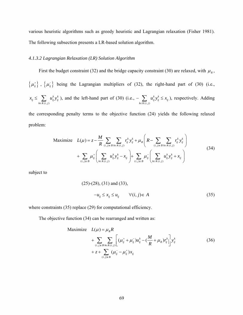
First the budget constraint (32) and the bridge capacity constraint (30) are relaxed, with R ,

ij , ij being the Lagrangian multipliers of (32), the right-hand part of (30) (i.e.,

( , )

k kij ij ij

k K i j

x u y

), and the left-hand part of (30) (i.e., ( , )

k kij ij ij

k K i j

u y x

), respectively. Adding

the corresponding penalty terms to the objective function (24) yields the following relaxed

problem:

( , ) ( , ) ( , ) ( , )

( , ) ( , ) ( , ) ( , )

Maximize ( ) k k k kij ij R ij ij

i j B k K i j i j B k K i j

k k k kij ij ij ij ij ij ij ij

i j B k K i j i j B k K i j

ML z r y R r y

R

u y x u y x

(34)

subject to

(25)-(28), (31) and (33),

( , )ij ij iju x u i j A (35)

where constraints (35) replace (29) for computational efficiency.

The objective function (34) can be rearranged and written as:

( , ) ( , )

( , )

Maximize ( )

( ) ( )

( )

R

k k kij ij ij R ij ij

i j B k K i j

ij ij iji j B

L R

Mu r y

R

z x

(36)

70

For any set of multipliers { } { } { }R ij ij , the relaxed problem is separable. First of

all, the first term RR is a constant. The second term ( , ) ( , )

( ) k k kij ij ij R ij ij

i j B k K i j

u r y

only

contains the variable kijy and constraints (31) and (33). Because k

ijy of different k are mutually

exclusive for any bridge ( , )i j , its value can be determined by the following equation:

( , )

( , ) ( , ) ( , )

max ( ) max ( )k k k k kij ij ij R ij ij ij ij ij R ij

k K i ji j B k K i j i j B

u r y u r

(37)

which can be solved by enumerating all elements in ( , )K i j . The third term ( , )

( )ij ij iji j B

z x

only contains variable ijx and z , and is a minimum cost flow problem with flow conservation

constraints (25)-(28) and capacity constraint (35). Such problem can be solved within

polynomial time (e.g., ( log )( log )O A N A N N as proposed by Orlin (1988). Therefore,

given any set of , the relaxed problem has the same computational complexity as a minimum

cost network flow problem and can be solved in polynomial time. The Lagrangian dual (LD)

min ( )L L

, which serves as an upper bound of the original NDP, can be solved efficiently by

iteratively solving the relaxed problem and updating the value of with methods such as the

subgradient method (Fisher 1981).

In every iteration, a heuristic feasible solution could also be obtained. ( ) kij ij iju can be

considered as the effectiveness of project ( , )i j k , incurring cost kijr . Given the budget R ,

various cost-effectiveness analysis methods (as described in the next section) can be applied to

identify the retrofit program y (Patidar et al. 2007). The maximum evacuation flow achieved by

retrofit program y is a lower bound of the original optimal flow. This lower bound can be solved

71

as a maximum flow problem*. The difference between the lower bound and the upper bound is

the optimality gap, which is the maximum possible difference between the current feasible

solution and the real optimum.

The LR method does not always yield an exact optimum solution, especially when the scale

of the problem is large. If needed, the LR algorithm can be incorporated into a branch and bound

framework (Ahuja et al. 1993) to reduce the optimality gap. However, as shown in the next

section, the solution for each scenario is only used as an estimation of the effectiveness of

projects, and hence obtaining the exact optimality is not ultimately important.

4.1.4 Effectiveness Measurement and Project Selection

The solutions to NDP for all S scenarios are used to compute the effectiveness of projects,

kijee from (20). The elements in function *( )se y are defined as:

:

, ( , ) , ( , ) \ 0k kij ij

k k kij ij ij

k u u

e r y i j B k K i j

, (38)

where kije is the effectiveness of project ( , )i j k in a single scenario, and the projects with 0k

(the “do-nothing” benchmarks) are not included in the computation. The effectiveness, kije , is

calculated as the average value of all kije across all scenarios.

In light of the project mutually exclusive constraints (31), it can be seen from (38) that in a

certain scenario, k k k kij ij ij ije r y r if project ( , )i j k is selected by NDP, i.e., 1k

ijy . This is based

on the assumption that if a project is selected, it shall at least provide a relative effectiveness

measure comparable to its cost; i.e., kijy is conceptually analogous to an effectiveness/cost ratio.

* When y is fixed, the NDP model reduces to a maximum flow model (with decision variables x and (24)-(30)), which calculates the maximum evacuation flow under retrofit program y . This problem can be solved by standard

network flow algorithms in polynomial time (e.g., Edmonds and Karp 1972).

72

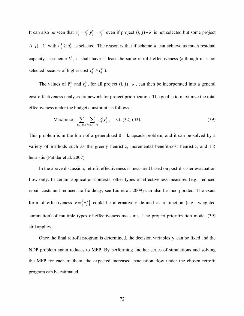
It can also be seen that k k k kij ij ij ije r y r even if project ( , )i j k is not selected but some project

( , )i j k with k kij iju u is selected. The reason is that if scheme k can achieve as much residual

capacity as scheme k , it shall have at least the same retrofit effectiveness (although it is not

selected because of higher cost k kij ijr r ).

The values of kije and k

ijr , for all project ( , )i j k , can then be incorporated into a general

cost-effectiveness analysis framework for project prioritization. The goal is to maximize the total

effectiveness under the budget constraint, as follows:

( , ) ( , )

Maximize k kij ij

i j B k K i j

e y , s.t. (32)-(33). (39)

This problem is in the form of a generalized 0-1 knapsack problem, and it can be solved by a

variety of methods such as the greedy heuristic, incremental benefit-cost heuristic, and LR

heuristic (Patidar et al. 2007).

In the above discussion, retrofit effectiveness is measured based on post-disaster evacuation

flow only. In certain application contexts, other types of effectiveness measures (e.g., reduced

repair costs and reduced traffic delay; see Liu et al. 2009) can also be incorporated. The exact

form of effectiveness kijee could be alternatively defined as a function (e.g., weighted

summation) of multiple types of effectiveness measures. The project prioritization model (39)

still applies.

Once the final retrofit program is determined, the decision variables y can be fixed and the

NDP problem again reduces to MFP. By performing another series of simulations and solving

the MFP for each of them, the expected increased evacuation flow under the chosen retrofit

program can be estimated.

73

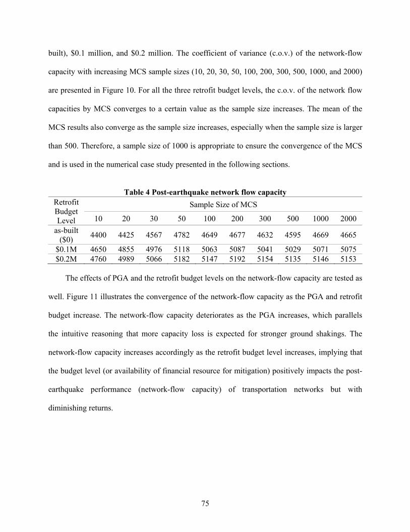
4.1.5 Convergence Tests

This section discusses the convergence of the network-flow capacity algorithms. The

Sioux-Falls network, one of the widely used benchmark networks in transportation engineering,

is assumed to have only ten bridges so the proposed algorithms can be investigated. The Sioux-

Falls network consists of 24 nodes and 76 edges, as shown in Figure 9. Nodes 1, 2, and 3

(illustrated by red circles in Figure 9) are assumed to be the seriously impacted area or

evacuation zones, and nodes 7, 18, 19, 20, and 21 as the safe zones (marked by green circles in

Figure 9). The network has 10 bidirectional bridges and the detailed bridge information is

described in Table 1, including the node numbers that indicate the location of each bridge, the

structure type, length, and PGA level, etc. These bridges are susceptible to earthquake and

limited resource shall be allocated to mitigate potential functional losses by retrofitting these

bridges. Road capacities are converted from the damage states of bridges according to the bridge

fragilities and bridge functionality relationships, as described in Chapter 3.

74

Figure 9 Sioux-Falls network for convergence test

Table 3 Bridge information for convergence test

Bridge ID

Node i

Node j

Structure Type

Structure Length (m)

Deck Width (m)

PGA (g)

1 4 5 MSC Steel 150 30 0.5 2 10 16 MSC Steel 150 30 0.5 3 12 11 MSC Steel 150 30 0.5 4 15 19 MSC Steel 150 30 0.5 5 14 15 MSC Steel 150 30 0.5 6 10 15 MSC Steel 150 30 0.5 7 11 14 MSC Steel 150 30 0.5 8 17 19 MSC Steel 150 30 0.5 9 23 24 MSC Steel 150 30 0.5 10 14 23 MSC Steel 150 30 0.5

The convergence of MCS is tested with the 10-bridge Sioux-Falls network. The post-

earthquake system performance (measured in terms of network-flow capacity) that results from

the optimal retrofit plan was show in Table 4 for three retrofit budget levels, namely, $0 (as-

75

built), $0.1 million, and $0.2 million. The coefficient of variance (c.o.v.) of the network-flow

capacity with increasing MCS sample sizes (10, 20, 30, 50, 100, 200, 300, 500, 1000, and 2000)

are presented in Figure 10. For all the three retrofit budget levels, the c.o.v. of the network flow

capacities by MCS converges to a certain value as the sample size increases. The mean of the

MCS results also converge as the sample size increases, especially when the sample size is larger

than 500. Therefore, a sample size of 1000 is appropriate to ensure the convergence of the MCS

and is used in the numerical case study presented in the following sections.

Table 4 Post-earthquake network flow capacity

Sample Size of MCS Retrofit Budget Level 10 20 30 50 100 200 300 500 1000 2000

as-built ($0)

4400 4425 4567 4782 4649 4677 4632 4595 4669 4665

$0.1M 4650 4855 4976 5118 5063 5087 5041 5029 5071 5075 $0.2M 4760 4989 5066 5182 5147 5192 5154 5135 5146 5153

The effects of PGA and the retrofit budget levels on the network-flow capacity are tested as

well. Figure 11 illustrates the convergence of the network-flow capacity as the PGA and retrofit

budget increase. The network-flow capacity deteriorates as the PGA increases, which parallels

the intuitive reasoning that more capacity loss is expected for stronger ground shakings. The

network-flow capacity increases accordingly as the retrofit budget level increases, implying that

the budget level (or availability of financial resource for mitigation) positively impacts the post-

earthquake performance (network-flow capacity) of transportation networks but with

diminishing returns.

76

0 200 400 600 800 1000 1200 1400 1600 1800 20000.08

0.11

0.14

0.17

0.2

Sample Size

Co

effi

cien

t o

f V

aria

tio

n

$0 budget$0.1 M budget$0.2 M budget

Figure 10 Convergence test of Monte Carlo sampling for network flow capacity

0.3 0.4 0.5 0.6 0.7 0.8 0.9 14000

4200

4400

4600

4800

5000

5200

5400

PGA (g)

Net

wo

rk F

low

Cap

acit

y

$0 budget$0.1 M budget$0.2 M budget$0.3 M budget

Figure 11 Convergence test of network flow capacity

4.1.6 Sensitivity to Ground Motion Correlation

The modeling of correlation of seismic ground motion has attracted renewed interests. It

has been recognized that uncertainties and correlation of ground motion is important to

accurately estimate the response of spatially distributed infrastructure systems (e.g.,

transportation and utility networks) and the associated economic losses (Bommer and Crowley

77

2006; Adachi and Ellingwood 2007; Lee and Kiremidjian 2007; Park et al. 2007; Zerva 2008).

The physical causes of spatial variation include: (i) the wave passage effect, (ii) extended source

effect, (iii) scattering effect (or ray path effect), and (iv) the attenuation effects (Zerva 2008).

Although the spatial variability has been accounted for extended structures (e.g., bridges)

(Burdette et al. 2008; Burdette and Elnashai 2008; Sextos, Pitilakis, and Kappos 2003), the

uncertainties of ground motion prediction in lifeline earthquake engineering are often

disregarded in deterministic seismic risk analysis, in which only the medians of ground motion

were used to obtain the best estimate or the mean value of risk (Zhou 2006). Additionally, the

spatial dependence of the site-to-site ground motions has not been extensively investigated (Park

et al. 2007) and majorly done with Monte Carlo simulations (Park et al. 2007; Bommer and

Crowley 2006).

This section discusses the effects of ground motion correlation and uncertainties on the

performance of transportation systems. The detailed procedures for generating seismic motions

that incorporate uncertainties and spatial correlation are described in Appendix C. In this analysis,

a magnitude 8.0 event on a hypothetical Sioux Falls vertical rupture plane is used for illustrative

purposes. The next generation attenuation (NGA) relationship by Campbell and Bozorgnia (2007)

is used to determine the distribution of median ground motion intensity (e.g., PGA) at each site

on the Sioux-Falls road network (Figure 12).

The effects of uncertainty and correlation of ground motions on the response of spatially

distributed infrastructure systems are studied in the 10 cases listed in Table 5. The first case

(Case I) does not consider the inter-event ( 1 0 ) or intra-event ( 2 0 ) and only uses the

median PGAs when generating the spatial distribution of ground motions. The ground motions in

78

the other nine cases share the same medians with the first case but are involved with the

uncertainties and correlation.

Figure 12 NGA hazard map (M8.0) and the Sioux-Falls road network

Table 5 Effects of ground motion uncertainty and correlation on system performance

Case No. 1 2 1 2b b

(km) Network flow

capacity (as-built)Network flow

capacity ($0.3 M)

I 0 0 n/a 3664 4486 II 0.1 0 n/a 3554 4378 III 0.3 0 n/a 3273 4152 IV 0 0.1 1 3681 4486 V 0 0.3 1 3621 4414 VI 0 0.3 15 3664 4486 VII 0.3 0.1 1 3289 4152 VIII 0.1 0.1 1 3569 4395 IX 0.3 0.3 1 3240 4089 X 0.1 0.3 1 3566 4390

79

Cases II and III assume no intra-event uncertainty ( 2 0 ) and only consider the inter-

event uncertainties ( 1 0.1 and 0.3 , respectively). The performance of transportation systems

(i.e., network flow capacity) tends to decrease as 1 increases.

Cases IV, V and VI assume no inter-event uncertainty ( 1 0 ) and focus on the intra-event

uncertainties. The simulation results show that the effect of intra-event uncertainty is not

significant—the performance of network flow capacity deteriorates slightly when increasing the

intra-event uncertainty and the correlation length. In fact, the effect of intra-event uncertainty is

trivial (about 1.6%) on the system performance, as illustrated in the Cases IV and V. Since

shorter correlation distance tends to represent the actual case more closely (Shinozuka et al. 2005;

Zhou 2006), a relatively small correlation distance ( 1 2 1b b km) is used in the other cases

when considering the intra-event uncertainty.

Both inter- and intra-event uncertainties are considered in Cases VII-X. The network

performance varies when introducing the inter- and intra-event uncertainties. The effects of these

uncertainties are similar to those in the cases in which only the inter-event uncertainties (Cases II

and III) or the intra-event uncertainties (Cases IV, V, and VI) are separately considered. That is,

the network flow capacity of transportation systems tends to decrease as 1 increases; and higher

intra-event uncertainty would result in smaller network flow capacity. Moreover, the comparison

of network flow capacities under the zero (as-built) and $0.3 M budget levels (Table 5) confirms

the positive impacts of the availability of budget for mitigation on the post-earthquake

performance of transportation networks.

80

4.1.7 Numerical Case Study: the Memphis Road Network

The Midwest region of the United States is an important “hub” of the nation’s

transportation systems. According to the 2002 Commodity Flow Survey by the Bureau of

Transportation Statistics (BTS), more than 968 billion ton-miles, or about 31% of the total U.S.

commodities originate, pass through, or arrive in the Midwest region (BTS 2005). The greater

metropolitan areas of Memphis are particularly of significance. With regard to freight, the

Federal Express Corporation (FedEx) worldwide headquarters and world hub are located in

Memphis. The third largest U.S. cargo facility of the United Parcel Service, Inc. (UPS), also the

only UPS facility capable of processing both air and ground cargo, is located in Memphis

(Hanson 2007); and the Memphis International Airport has been the world’s busiest airport in

terms of cargo traffic volume. On the passenger side, the City of Memphis and surrounding

metropolitan area is one of the two major population centers in the Midwest U.S. The greater

Memphis metropolitan area, however, is one of the most vulnerable regions to seismic hazards in

the U.S. The aging infrastructure and many unreinforced buildings would sustain significant

damage and more than one million population severely impacted. A catastrophic NMSZ

earthquake could not only disrupt the direct functioning of the Memphis metropolitan area but

also have ripple effects throughout the nation’s economy and society.

The numerical case study focuses on the road network in the Memphis metropolitan area.

The road network information (e.g., node and link characteristics) is collected from the local

metropolitan planning organization (MPO)—the Memphis Metropolitan Planning Organization.

Figure 13 illustrates the 12,821 nodes, 15,758 links, and 616 bridges in the Memphis network.

Detailed bridge information, including the location, structure length, and deck width, etc. is

retrieved from the 2002 National Bridge Inventory (NBI) database, which is maintained by the

81

U.S. Department of Transportation and FHWA. The NBI is a collection of information covering

around 600,000 bridges on the public roads in the U.S., containing detailed information on the

bridge characteristics such as location, year of built, geometry, material, construction, and

conditions (FHWA 1995a). For the purpose of demonstrating the proposed methodology, all the

bridges are assumed the same structural type (i.e., multi-span simply supported steel). Based on

the “seismic emergency routes” for seismic events in west Tennessee by the Tennessee

Emergency Management Agency (TEMA) (Duncan 2008; Leatherwood 2008; Seger 2008) and

the seismic risk assessment of the New Madrid Seismic Zone (Elnashai et al. 2009), network

nodes inside the dotted box are assumed to be evacuation zones (i.e., disaster-impacted areas),

and the nodes marked with circles to the east and south of the target area are assumed safe zones.

The local streets are assumed to have only 10% of their normal capacity after earthquake while

higher-level roadways such as highways and major arterials can keep 100% capacity (Zhou et al.

2004), implying the local streets may not be suitable for evacuation after a seismic event (Kim et

al. 2008) and the target network would be short of detour routes after a major seismic event

(Zhou et al. 2004).

This research uses a M7.7 earthquake on all the three fault segments simultaneously, which

is advised by the USGS as the most appropriate NMSZ “characteristic” event. This characteristic

earthquake is taken as a representative event to identify the bridge residual capacity scenarios.

The USGS ground shaking maps with 7-10% probability of exceedance in 50 years (Schweig

2008; Cramer 2006) are used to estimate the bridge damages caused by the earthquake impact.

Figure 14 illustrates the spatial distribution of the medians of PGA. The capacities of the links

with a bridge are calculated from the damage states of bridges according to the bridge

functionality relationships and bridge fragilities. As an example, Figure 15 illustrates the fragility

82

curves of the multi-span simply supported (MSSS) steel bridges with and without a retrofit

scheme (e.g., elastomeric bearing).

Figure 13 Road network in the Memphis metropolitan area, Tennessee

The bridge retrofit cost estimates (per unit bridge deck area) are obtained based on personal

communications with several bridge engineers in the Tennessee and Illinois Departments of

Transportation (DesRoches 2008). Five different retrofit schemes are considered, including

elastomeric bearing, restrainer cable, seat extender, shear key, and steel jacket. In practice, these

retrofit schemes do not necessarily have a strict domination relationship between on another

83

since the retrofit effectiveness also depends upon the bridge type and damage state (Padgett

2007).

Figure 14 Seismic hazard map for Memphis MPO (the M7.7 NMSZ earthquake scenario)

Figure 15 Fragility curves of multi-span simply supported (MSSS) steel bridges

NDP is solved by the commercial solver CPLEX® at five budget levels, each based on

1,000 earthquake scenarios generated by MCS. Here 10M so the accuracy of NDP is 10

84

vehicles per hour. The maximum allowable optimality gap for NDP is set to be 0.000001%. The

total solution time for all five budget levels is about 3000 seconds on a personal computer with 2

GHz CPU and about 60 MB of memory usage. The retrofit project effectiveness is a weighted

summation of the expected evacuation flow (now denoted by kFije ) and the expected reduction in

repair cost (denoted by kRije )†; i.e., k k k

ij Fij Rije we e . The weight is set as 100w , such that the

total effectiveness of evacuation flow is about the same as that of the reduced repair costs for

those bridges selected at least once in 1000 scenarios. In practice, other types of effectiveness

measures (e.g., long-term transportation operation efficiency) can also be considered.

The top 20 bridges with the highest effectiveness/cost ratio in the retrofit program list are

shown in Table 6. These bridges have higher effectiveness/cost ratio because they are at the most

vital location of the network and/or are more vulnerable to earthquakes. A simple yet efficient

greedy heuristic is used to select the retrofit projects. Retrofit projects are checked one by one

from the highest effectiveness/cost ratio to the lowest before the budget is exhausted. If two

retrofit schemes are selected for the same bridge during the process, the one with higher

effectiveness will be used. Other cost-effectiveness analysis methods can be found in Patidar et

al. (2007).

Table 6 Top 20 bridges with highest effectiveness-cost ratios

Budget (in millions) / Bridge ID‡ Rank

$0.2 $0.4 $0.6 $0.8 $1.0 I 237 237 237 237 237 II 157 157 157 157 157 III 110 110 110 110 110 IV 139 139 139 139 139 V 138 138 138 138 138

† See Appendix A for the detailed definition of k

Rije . ‡ Bridges with varying cost/effectiveness ratio at various budget levels are in bold font.

85

Table 6 (cont.) Budget (in millions) / Bridge ID

Rank $0.2 $0.4 $0.6 $0.8 $1.0

VI 31 31 31 31 31 VII 259 259 259 259 259 VIII 30 146 146 146 146 IX 146 30 30 30 30 X 256 256 256 256 256 XI 137 137 137 137 137 XII 135 135 135 135 135 XIII 147 147 147 147 147 XIV 255 255 255 255 255 XV 589 142 142 142 142 XVI 142 589 589 589 589 XVII 136 52 143 143 143 XVIII 143 136 52 136 136 XIX 217 143 136 62 62 XX 52 62 62 52 52

Figure 16 shows the spatial distribution of the retrofitted bridges selected by greedy

heuristic with a budget of $1 million. It can be seen that most retrofitted bridges are close to the

safe zones. The reason is that the road network is much denser near the city, and the traffic is

able to evacuate through minor highways that do not have a bridge. However, if the study area

was expanded and the safe zones moved farther away from the city, it is expected that the

retrofitted bridges concentrate somewhere between the city and the safe zones. The reason is that

the bridges far from the city turn out to bear lower earthquake intensity and thus are less likely to

be damaged—retrofitting these bridges is relatively less beneficial. Generally, the selection of

projects depends on many factors such as the effectiveness measures, the topology of the road

network, the location of evacuation and safe zones, and the earthquake intensity distribution.

In order to plot the relationship between effectiveness and budget, the effectiveness of

retrofit programs (i.e., the total effectiveness of retrofit projects in a program) at various budget

levels should be calculated. It can be seen from Table 6 that the order of the bridges sorted by

86

effectiveness/cost ratio only changes slightly across different budgets (the bridges with different

ranks at various budget levels are highlighted by bold font). Therefore, the effectiveness

calculated from the $1 million budget case can be used to create retrofit programs in other

budgets (including the zero budget case) without losing much accuracy. For each budget, greedy

heuristic is used to select the retrofit projects. The greedy algorithm terminates as soon as the

cost of the currently checked project exceeds the remaining budget, and then the budget is

recalculated as the sum of the costs of all selected retrofit projects. In this way, it can be ensured

that there is no remaining budget and the created retrofit program is optimum.

Figure 16 Spatial distribution of bridge retrofit program under $1 million budget

87

Twenty-one retrofit programs are proposed and then tested with another 1,000 earthquake

simulation scenarios. The average effectiveness of both evacuation flow rate and the reduced

repair costs at various budget levels are illustrated in Figure 17. The trend shows that higher

budget has positive effects on the retrofit effectiveness. However, the increase of the budget has

diminishing returns; the effectiveness (i.e., maximum flow rate and the reduced repair costs)

curve becomes flat when the budget exceeds about $0.8 million. This curve can help the

decision-making agencies choose appropriate budget level based on factors such as evacuation

plan and available budget.

Figure 17 Budget-effectiveness curves

4.1.8 Discussion

This numerical case study focuses on the bridge seismic retrofit program planning and

proposes an OD-independent method to calculate the evacuation flow effectiveness. The

uncertainties of earthquake intensities are addressed with a Monte Carlo simulation framework.

The evacuation flow effectiveness in each simulated scenario is calculated based on a network

design model, and the retrofit program is decided by using cost-effectiveness analysis. Note the

88

scope of evacuation is limited to the short-term period and steady-state flows and the evacuation

zones are assumed to have sufficient demands during the evacuation process.

The proposed methodology is demonstrated with a real-world case study in the Memphis

metropolitan area. Results from the numerical example show that the effectiveness of retrofit

programs increases with the budget with diminishing returns. Specifically, the maximum flow

rate is positively correlated with the reduced repair costs, which increases linearly with the

available budget. The results from the case study also suggest the presence of optimum amount

of allocated resources (i.e., critical level of budget), beyond which additional retrofitting

becomes less effective. The budget-effectiveness curve is consistent with the intuition that higher

budget levels lead to more retrofit effectiveness but with diminishing effectiveness.

The demonstrated network-flow capacity-based NBSR methodology can be used to (i)

evaluate post-earthquake performance of transportation systems, (ii) identify retrofit project

priorities, (iii) plan budget from a systematic viewpoint, and (iv) improve the disaster resilience

of transportation systems under economic constraints. The proposed methodology also allows

more general effectiveness measurements to help government agencies and emergency managers

make better decisions.

4.2 Reliability of Network Reachability

This section discusses the reliability of network reachability of transportation infrastructure

systems by employing the recursive decomposition algorithm. In an emergency, it is critical to

identify the passable ingress and egress routes for emergency response within a short time frame,

e.g., to send search and rescue teams into the impacted area immediately after a disruptive

earthquake. To emergency managers and rescue workers, of great concern are the knowledge of

potential bridge collapse or road closure due to seismic impact, and whether the structural

89

damage interrupts the integrity or connectivity of transportation systems. The reliability of

network reachability is an appropriate metric under such conditions.

4.2.1 Recursive Decomposition Algorithm for Reachability Reliability

Figure 18 illustrates the key RDA procedures to evaluate the system reliability by

decomposing a simple benchmark network. To evaluate the network connectivity between the

source node s and terminal node t (e.g., the impact zone and safe zone), first an arbitrary

shortest path { 1 2 }s t between the source and terminal is identified. Based on the

identified path, the network is then decomposed recursively into sub-graphs until there is no path

existed between the source-terminal node-pair in all sub-graphs. For the benchmark network

shown in Figure 18, the RDA identifies five disjoint link sets { 1 1 2L , 2 1 4 5L ,

3 1 2 4 5L , 4 1 4 5 3 2L , 5 1 2 4 3 5L } and six disjoint cut sets { 1 1 4F ,

2 1 2 4 5F , 3 1 4 5 3F , 4 1 4 5 3 2F , 5 1 2 4 3F , 6 1 2 4 3 5F }, in which

the numbers with and without an upper bar indicate the failures and survivals of the

corresponding network components (e.g., edges), respectively.

Before applying the RDA to the numerical case study, its correctness of implementation is

verified by comparing the system accessibilities between the source node and sink node for

twenty commonly-used benchmark networks. The verification of the RDA is detailed in

Appendix B.

90

3 1 2 4 5L

4 1 4 5 3 2L 5 1 2 4 3 5L 1 1 4F 2 1 2 4 5F

3 1 4 5 3F 4 1 4 5 3 2F 5 1 2 4 3F 6 1 2 4 3 5F

1 1 2L

2 1 4 5L

Figure 18 Illustration of the recursive decomposition algorithm

4.2.2 Numerical Example: the Sioux-Falls Road Network

The RDA is illustrated by using the Sioux-Falls network (shown in Figure 19) as a

numerical example. The bridge information is described in Table 3. The impacted zones (i.e.,

evacuation zones) are considered the source nodes and a virtual sink node is added to the graph

to facilitate finding the node-pair connectivity for the multi-source and multi-terminal network

model. The failure probabilities of bridges are calculated by using the bridge fragility curves and

the hazard maps given in Section 4.1.5.

Figure 20 shows the probability that the impacted zone (i.e., Node 1) will be disconnected

from safe zones. Note that the consideration of spatial correlation of ground motion affects the

estimates of system reliability but not significantly. An additional investigation on the correlation

of structural damage would be necessary to obtain more reliable results, but is beyond the scope

of this study. Figure 21 gives the disconnection probabilities of several selected network nodes,

in which the intra-event uncertainty 2 is 0.1 and the correlation length b is 4 km.

91

Figure 19 Sioux-Falls network for network reachability

5 5.5 6 6.5 7 7.5 8

0.35

0.4

0.45

0.5

0.55

0.6

Earthquake Magnitude

Dis

conn

ect

ion

Pro

ba

bilit

y o

f N

ode

1

b = 0km

b = 4km

b = 10km

b = 30km

Figure 20 Probability of disconnection (node 1)

92

5 5.5 6 6.5 7 7.5 80.25

0.3

0.35

0.4

0.45

0.5

0.55

0.6

0.65

Earthquake Magnitude

Dis

con

ne

ctio

n P

roba

bilit

y

Node 1Node 3Node 4Node 9

Figure 21 Nodal disconnection probability

4.2.3 Case Study: the Memphis Road Network

For the purpose of illustrating the methodology and reducing undue complexity, this

numerical case study focuses on a simplified road network that only contains major highways in

Shelby County and the City of Memphis, Tennessee. In order to apply the RDA to the simplified

Memphis road network, first the network is represented with a digraph model with a subjunctive

sink node added to the graph, as shown in Figure 22 (details of numbering are not included).

Nodes 11, 15, 16, 17, 18, 26, 28, 29, 32, and 33 (inside the dotted oval) are assumed to be

evacuation zones (i.e., disaster impacted areas), and nodes 4, 34, 10, 20, and 24 are safe zones.

The choice of evacuation pattern is made based on the “seismic emergency routes”, which are

designated by the TEMA (Duncan 2008; Leatherwood 2008; Seger 2008). Seismic reliability of

the network components under given earthquake excitations can be evaluated using structural

fragility curves. For demonstration purpose, the reliabilities of all components (except for the

added virtual sink) are assumed 0.9, 0.7, and 0.5 in the respective cases.

93

Figure 22 Simplified Memphis road network with the subjunctive sink

4.2.4 Results and Discussion

The network reachability between the safe zones to each of the evacuation zone is given in

Table 7 and Figure 23. The connectivity reliabilities of the impacted zones are then illustrated in

the GIS environment. Figure 24 shows the system reachability reliability of the road network in

Shelby County and the City of Memphis, Tennessee.

Table 7 Network reachability with convergence criteria of 0.001

Number of Link Sets Number of Cut Sets Reachability Reliability Node No. Case

I Case

II Case III

Case I

Case II

Case III

Case I

Case II

Case III

11 1063 1076 1054 3837 3873 3814 0.872 0.430 0.087

15 1 1 1 5 5 5 0.656 0.240 0.063

16 1 1 1 4 4 4 0.729 0.343 0.125

17 1 1 1 7 7 7 0.531 0.118 0.016

18 1 1 1 6 6 6 0.591 0.168 0.031

26 40 45 45 99 110 104 0.783 0.340 0.076

28 2251 2274 2191 7428 7489 7289 0.886 0.477 0.112

Subjunctive Sink

94

Table 7 (cont.)

Number of Link Sets Number of Cut Sets Reachability Reliability Node No. Case

I Case

II Case III

Case I

Case II

Case III

Case I

Case II

Case III

29 1063 1076 1017 3832 3871 3709 0.785 0.301 0.044

32 1 1 1 8 8 8 0.478 0.082 0.008

33 42 47 45 99 110 109 0.871 0.486 0.151

Figure 23 Reachability reliabilities of network nodes

Figure 24 Reliability of reachability to safe zones (case II)

95

This approach is capable of handling large infrastructure systems—in essence, it reduces

the size and complexity of the large urban infrastructure systems by decomposing the complex

system into sub-systems whose reliabilities are easy to evaluate. The illustrated approach

provides useful information for not only the TMA and users of transportation systems, but also

emergency managers to make informed decisions for timely response and relief.

Note that this reachability algorithm does not account for dependence within the

components due to the common source of earthquake. The availability of complete information

about the system is also assumed for illustrative purpose. Nevertheless, the spatial correlation of

the network damage can be addressed by the MSR method (Song and Kang 2007) or Bayesian

network (Friss-Hansen 2004), which can account for incomplete information and give results

such as conditional probability and importance measures (Song and Kang 2007).

4.3 Summary

The chapter discusses the evaluation of transportation systems with the OD-independent

performance metrics that are identified in Sections 3.5.1 and 3.5.2. The network flow capacity

metric is used to measure the system performance of a transportation network under emergency

conditions. This performance metric of network flow capacity avoids the dependence on the OD

data, and hence overcomes the critical limitation of the unrealistic assumption on post-disaster

travel pattern.

A NDP-based mathematical model for optimal retrofit programming is proposed and an

efficient solution algorithm is developed under the MCS framework. The convergence of MCS

and the sensitivity to input parameters are tested as well. The network flow capacity-based

approach is demonstrated with a real-world case study of the Memphis road network.

96

In addition, the network reachability, or the connectivity reliability between the safe zones

and evacuation zones is discussed and a sensitivity analysis is performed for relevant factors.

The network reachability of the Memphis road network is quantified by employing the state-of-

the-art RDA. Based on such results, the regions that are potentially difficult to reach after a

disruptive earthquake can be identified to make informed emergency response plans.

The proposed OD-independent performance metrics extend the existing NBSR framework

and provide essential information for emergency response, efficient retrofit prioritization, and

budget planning procedures. The following chapter, Chapter 5 discusses post-earthquake travel

demand modeling and evaluates the performance of transportation networks with the travel delay

cost metrics.

97

CHAPTER V MODELING THE POST-EARTHQUAKE TRAVEL DEMAND

5.1 Introduction

The state-of-the-art seismic mitigation measures for transportation systems have focused on

earthquake design and retrofit of transportation infrastructure. In emergency situations, however,

the operation of highway systems is equally important. The traffic flow under emergency

conditions (e.g., a damaging earthquake) may be significantly different from the traffic under

“normal” conditions due to the drastic changes in post-event demand and the deteriorated

network capacities as well. Conventional travel demand models such as the FDM are limited and

unsuitable in post-earthquake emergency situations due to unrealistic assumptions (Shinozuka et

al. 2005; Fan 2006; Werner et al. 2006; Kiremidjian et al. 2007).

Employing travel delay cost metrics for the performance evaluation of transportation

systems, this chapter focuses on the development of demand simulation models that account for

the change of traffic pattern after a damaging earthquake. Because travel delay cost metrics are

highly dependent upon the detailed OD travel demand information, a methodology to model the

post-earthquake travel demand is first given in Section 5.2. This model approximates the

“abnormal” travel demand by adopting several general principles. The post-earthquake travel

patterns are characterized by considering the effects of structural damage and emergency

facilities on travel behavior. Section 5.3 presents the results from the numerical case studies, in

which the performance is measured by the travel delay cost metrics. Section 5.4 discusses the

results and summarizes the major conclusions.

98

5.2 Methodology for Travel Demand Modeling

Based on the review of travel demand models and post-earthquake travel patterns in Section

2.2.1.3, this section presents a methodology to model post-earthquake travel demand and

evaluate the system performance with travel delay cost metrics. Note the proposed methodology

does not attempt to provide “real-time” post-earthquake traffic simulation. Instead, it aims at

providing general principles and procedures for emergency training and planning purposes. The

major assumptions and key procedures of the proposed methodology are presented in the

following subsections.

5.2.1 Scenarios and Major Assumptions

Earthquake occurrence time significantly affects the number of casualties and their spatial

distribution since traffic patterns and population distribution in different periods are distinct. For

this reason, useful earthquake scenarios for demand modeling should specifically consider the

occurrence time of day (e.g., morning and late-night period), days of the week, and the seasons

of the year, etc.

In this study, two hypothetical scenarios are developed to postulate and model the impact of

a no-notice event on transportation systems—one occurring during morning rush hours

(hereinafter referred to as the day scenario), and another at late night (hereinafter referred to as

the night scenario). Both scenarios are assumed to occur without the presence of adverse weather

conditions such as rain or snow. The hypothetical scenario earthquakes will leave several bridges

(e.g., major river crossings) and essential facilities (e.g., schools) severely damaged. Traffic

management measures may include closures of highways due to damages of ramps or pavements,

demolished or severely undermined bridges, or evacuation of regions with HAZMAT release, etc.

These scenarios can provide emergency response teams with optimal transportation pathways for

99

rapid emergency ingress and egress, and help evaluate emergency routes performance and

estimate congestion under extreme events.

Modeling travel behavior and route choices, even under normal conditions, is challenging.

Approximation of travel demand following earthquakes is challenging due to many socio-

economic uncertainty aspects involved (Fan 2006). To simplify the complex problem of travel

demand modeling, several general assumptions are made on post-earthquake travel behavior and

emergency traffic management measures (Chang et al. 2009):

This study assumes that people will evacuate directly from their current locations

immediately after earthquakes. This assumption is made because under pre-noticed

scenarios such as hurricane evacuation (e.g., 24 or 48 hours before the landfall), it is

reasonable to assume that people will be either at home, or returning home before

beginning the evacuating. While under the no-notice earthquake scenarios, there is

no time or considerably less time to return home or go to other places to pick up

their relatives or friends (Noh et al. 2009). Social vulnerability to disasters such as

race, gender, and social inequality has a crucial role in shaping the evacuation

patterns, but is beyond the scope of this study.

Trip generation is assumed proportional to the size of affected population, and trip

generation rates common within the TAZ. Such homogenous assumption on the

TAZ is based on the cross-classification methods, which aggregate the population

into certain homogenous groups based on their geographic locations and socio-

economic characteristics such as auto ownership and income, etc. (EWGCC 2003;

Chatterjee and Venigalla 2004). Moreover, because the pattern of population

distribution changes at different periods of time, the number of population during

100

day time and at night, if available, will be taken from the 2000 U.S. census for the

trip generation of the morning scenario and late night scenario, respectively.

Depending on the presence of attractants (e.g., hospitals or emergency shelter) and

repellents (e.g., HAZMAT release, fire following earthquake, or damaged facilities),

the TAZ can be classified into four zone types (Figure 25). The underlying

assumptions are that: (i) if a zone does not have damaged facilities, its trip

production will not be affected by the earthquake, while the trip production will

increase in the affected zones due to facilities damage, fire or hazmat release, and (ii)

if a zone does not offer emergency shelters or hospitals, its trip attraction will

remain unchanged; while the trip attraction will increase because of the presence of

emergency shelters and/or hospitals. Figure 26 illustrates the assumptions on zone

types and Table 8 summarizes the characteristics of trip generation for each of the

zone type.

Bridges with at least major damage are assumed to be impassable and closed

(Yashinsky 1998). Buildings with at least moderate damage will be evacuated§.

Special group population in schools and colleges, hospitals, and jails may be

required to evacuate due to structural damage (Schultz et al. 2003).

Neighboring region of HAZMAT release due to the damage to HAZMAT plants or

explosion of nuclear power plants requires a full evacuation. Emergency shelters

and hospitals are assumed attractive sites to injured or displaced people. The

attracted trips to shelters and hospitals are proportional to their capacities (e.g., the

number of beds in a hospital).

§ Due to the lack of specific population/square footage information for individual buildings　 , two additional assumptions are made: (i) damage is evenly distributed across occupancy types, and (ii) population or square footage is evenly distributed within the same occupancy category.

101

No Repellency Present

AttractionsPresent

No AttractionsPresent

RepellencyPresent

RE

PE

LL

EN

CE

AT

TR

AC

TIO

N

2

1

3

4

Figure 25 Classification of zone types

Figure 26 Illustration of TAZ types

Table 8 Characteristics of zonal traffic generation

TAZ Number

Zone Type

Trip Production Trip Attraction Note

A I unchanged unchanged not affected

B II unchanged background +

attracted presence of hospital

and/or shelter

C III background +

evacuated background

reduction factor** presence of building damage

D IV background +

evacuated none presence of HAZMAT release

E IV background +

evacuated background +

attracted

presence of both hospital/shelter and HAZMAT release/building

damage

** Trip reduction rates at various ground motion intensities are interpolated from the maximum reduction factors of all trip purposes specified in Shinozuka et al. (2005).

102

5.2.2 Major Modeling Steps

The proposed approach for transportation systems modeling is developed based on the

classical urban transportation planning process (UTPP) models. As illustrated in Figure 27, the

proposed procedures start with the step of trip generation. In trip generation step, the total

number of trips produced and attracted by each TAZ is estimated. Trip generation is followed by

the integrated trip distribution/assignment step (Evans 1976). In this combined step, zone-to-

zone trip interchanges are first predicted by trip distribution models that generate a post-

earthquake trip matrix representing the spatial pattern of trips between origins and destinations;

and then post-earthquake trip matrix is loaded to the damaged road network to estimate traffic

flow and travel cost by using trip assignment models. The major steps of the procedure are

detailed in the following subsections.

Figure 27 Methodological framework for demand modeling and performance assessment

5.2.2.1 Trip Generation

Trip generation is the first step of traffic modeling, consisting of trip production and trip

attraction. The goal of trip generation is to estimate the number of trips that originate from and

arrive in each TAZ, i.e., to determine trip production and attraction by location and trip purpose.

103

Trip generation models have two fundamental structures: (i) cross-classification models of

trip rates at an aggregate (zonal) level, and (ii) regression models at an aggregate or disaggregate

(household or individual) level (Zhao and Kockelman 2002). The cross-classification models

classify the population into certain homogenous groups based on the socio-economic

characteristics such as household size, auto ownership, and income (EWGCC 2003; Chatterjee

and Venigalla 2004). In regression models, the trip rates are empirically estimated for each of the

classification. For example, the trip rates from the Institute of Transportation Engineers (ITE) are

based on land use and employment data. In the present study, zonal trip production and trip

attraction are calculated based on pre-earthquake “background” travel demand as well as the

characteristics of zonal attraction from emergency facilities and repellence due to building

damage and/or HAZMAT release, as illustrated in Figure 28 and Table 8. Note that the

discrepancy between the number of trip productions and attractions is not adjusted, because the

assumption on trip conservation (also known trip balancing) in normal conditions may not hold

under the “abnormal” post-earthquake situations.

Building Damage

General Building Stock

Evacuated Population/Trips

Trip Production

Essential Facility

Trip Attraction

Medical Care

Emergency Shelter

Attracted Population/Trips

Figure 28 Flowchart of trip generation

104

In this study, the generated trips related to residential buildings are assumed proportional to

the affected population in a TAZ. While trips related to commercial or industrial buildings are

assumed proportional to the affected square footage and are estimated using the ITE trip rates.

To estimate the travel demand stemming from structural damage, detailed information is

required on the composition of building inventory, the damage distribution amongst the

inventory, and the population associated with the damaged buildings. The attracted trips to

emergency shelters and hospitals are estimated based on their respective capacities, e.g., the

number of beds in a hospital and the post-impact capacity of an emergency shelter.

Travel demand (in the unit of vehicle trips) is aggregated at the TAZ level. Population data

is aggregated at census tract level, while the building damage information may be available only

at aggregated level, or at individual structure level for a limited areas††.

If the damage information is unavailable for individual buildings (i.e., the aggregated

damage case), the number of damaged buildings in each occupancy category can be estimated

based on the total number of damaged buildings in the census tract and the damage probability of

the structural fragility curves (Figure 29). Since the composition of building occupancy types is

unknown, it is assumed that the number of damaged buildings of certain occupancy type is

proportional to the exceeding probability of structural limit states specified in the representative

fragility curves. In other words, the more vulnerable (higher exceeding probability) the building

is to earthquake, the higher percentage (or more probable) of damaged buildings is in the

inventory. For example, given the ground motion intensity x , the exceeding probabilities are 0.4

and 0.85 (Figure 29) for concrete and wood structure, respectively. This means the number of

damaged residential buildings would be approximately 2.1 times of that of damaged commercial

†† Individual building damage information can be obtained only for the City of Memphis and Shelby County, Tennessee with the building inventory provided in MAEViz.

105

buildings. The number of damaged buildings of each occupancy category can then be estimated

with the exceeding probabilities given by the fragilities, followed by the estimation of the

increase of trips due to structural damage for each TAZ.

00

0.2

0.4

0.6

0.8

1

Intensity Measure (IM)

Ex

ceed

ance

Pro

bab

ilit

y

Figure 29 Structural fragility curves for the estimation of damaged buildings

5.2.2.2 Trip Distribution and Trip Assignment

Trip distribution and trip assignment steps are combined into a single step in the present

study, following Evan’s (1976) formulation of the combined assignment and distribution model.

Trip distribution models are used to predict zone-to-zone trip interchanges, i.e., the spatial

pattern of trips between origins and destines. While trip assignment models provide essential

information on traffic flow and travel delays due to excessive damage to key infrastructure

elements, or from the reduced traffic carrying capacity because of less severe damage (e.g., lane

closure for repair or imposed lower speed limit).

Gravity model is the most widely used trip distribution technique (Easa 1993; Chatterjee

and Venigalla 2004), and has been used to estimate the “abnormal” travel demand in extreme

events (Shinozuka et al. 2005; Zhou 2006; ORNL 2002; Chang 2003; Moriarty et al. 2007;

Fragility I (Residential-wood)

Fragility II (Commercial-concrete)

x

106

Wakabayashi and Kameda 1992). Other popular trip distribution models include the growth

factor models such as the Fratar Model and the Detroit Model. These growth factor models are

an extrapolation of the previously surveyed OD data by assuming that future transportation

distribution has similar pattern as the current one, and hence restricted to long-range forecasting

travel demand in an urban area. Since it is difficult to obtain post-earthquake OD data, gravity

model is employed to determine where trips go (trip distribution) in the present study.

The gravity model is in analogy with Newton’s law of gravity—the trip interchange

between origin and destination zones is proportional to activities represented by trip generation,

and inversely proportional to the separation (impedance) between the zones, which is usually

represented as a function of travel time. The gravity model, subject to the constraints of trip

production and trip attraction, is defined as follows:

( )i j

ij i jij

O DT A B

F t (40)

where ijT is the number of trips from zone i to zone j , iA is the constant to balance trips

originating from zone i , jB is the constant to balance trips destined for zone j , iO is the

number of trip production in zone i , jD the number of trip attraction in zone j , ijt the

impedance (travel time or cost) from zone i to zone j , and ( )ijF t the deterrence function,

which is usually inversely related the zone separation in a form of Gamma, power, or

exponential functions. This doubly constrained gravity distribution model ensures that the

resultant trip matrix matches the productions and attractions of each TAZ. The output trip matrix

(i.e., the post-earthquake travel demand) is then loaded to the transportation networks with traffic

assignment models to simulate the traffic flow over the roads following the earthquake.

107

Trip assignment, also known as traffic assignment, provides essential information of traffic

flow and travel costs. The travel delay cost metrics (e.g., TSTT) obtained by traffic assignment

models are used to measure the functional loss of transportation system. The Network Loss

Analysis (NLA) module in MAEViz, MAE Center’s comprehensive seismic risk assessment

package, is employed for simulating the post-disaster emergency traffic.

Both static and dynamic traffic assignment models are implemented in the NLA module

under the user equilibrium assumptions. The DUE model is one of the macro-simulators based

on equations stemming from analogies with fluid flows in network, and does not attempt to track

the behavior of individual vehicles and is. To ensure the correctness of the implementation of

DUE model, the TSTT results are first validated by checking their corresponding upper and

lower bounds (see Appendix D).

The DUE model is static and only copes with steady state conditions, which may not be

adequate in the dynamic, and sometimes chaotic environment of an emergency evacuation (Pidd

et al. 1996). In order to model the time-dependent traffic over the network, the NLA module

incorporates the Visual Interactive System for Transport Algorithms (VISTA), which is the state-

of-the-art DTA model built upon the enhanced CTM and supports for variable-sized cells and

signalized intersections (Ziliaskopoulos and Waller 2000).

5.3 Case Studies

5.3.1 Sioux-Falls Road Network

The proposed methodology is illustrated by the Sioux-Falls network (Figure 30) as a

numerical case study. Nodes 1, 2, and 3 are assumed to be the evacuation zones (i.e., impacted

area with building damage or HAZMAT release), and nodes 7, 18, 19, 20, and 21 to be the safe

zones with emergency shelters and/or medical facilities.

108

In order to characterize the unbalanced trip production and trip attraction patterns for

business zones (i.e., nodes 2, 9, 10, and 11) and residential zones (i.e., nodes 1, 3, 13, 18, and 19),

the traffic patterns in these zones are represented by asymmetric origin-destination matrices. The

modified origin-destination tables (Tables A4 and A5 in Appendix E) are taken as the pre-

earthquake “background” demand in the hypothetical scenarios. Additionally, the originally

identical link properties (e.g., traffic-carrying capacities and speed limits) are modified to

represent a generic road network—link-pairs 1-3, 7-35, 17-20, 25-26, 28-43, 59-61, and 34-40

(as marked in Figure 30) are chosen and their link traffic-carrying capacities and speed limits are

modified such that they are not identical for the selected link-pairs. Detailed link properties of

the modified Sioux-Falls network are described in Table A3 in Appendix E.

54

1

8

4 5 63

2

15 19

17

18

7

12 11 10 16

9

20

23 22

14

13 24 21

3

12

6

8

9

11

5

15

122313

21

16 19

17

2018

55

50

48

2951 49 52

58

24

27

32

33

36

7 35

4034

41

44

57

45

72

70

46 67

69 65

25

28 43

53

59 61

56 60

66 62

6863

7673

30

7142

647539

74

37 38

26

4 14

22 47

10 31

1

23

7 6

8

45

10

9

A

A

C

C

B

B

S

S

S

11

19

Business Zone

Residential Zone

Bridge

S

HAZMATRelease

Hospital

Emergency Shelter

Legend

Damaged Building

Direction of Egress Traffic

Direction of Ingress Traffic

Modified Link-pair

Figure 30 Sioux-Falls road network with evacuation and safe zones

109

The 10 bridges on the Sioux-Falls network are assumed to be multi-span simply supported

steel bridges. The vulnerability of roadways is not considered and bridges are assumed the only

vulnerable components to earthquake. The bridge traffic capacities are calculated by using the

bridge fragilities and bridge functionality relationships as described in Padgett (2007). For

demonstration purposes, the day-0 capacity values are taken as the traffic capacity immediately

after the earthquake (i.e., the worst case) to evaluate the impact on the Sioux-Falls network.

5.3.1.1 Network Congestion

Traffic congestions given by employing the static DUE models are illustrated in Figure 31

and Figure 32 for the respective scenarios, while Figure 33 and Figure 34 present the congestions

predicted with the DTA models. The congestion (also known as the level of service [LOS]) is

measured by the volume-capacity (v/c) ratio. Figure 31(a) illustrates the pre-earthquake

congestions for the Sioux-Falls network in the night scenario by using the DUE models. The

post-earthquake traffic congestions on the links connecting the impact zones and safe zone using

the proposed integrated assignment/distribution models (hereinafter referred to as integrated

models, or IM) are more significant than those predicted by the conventional fixed demand travel

simulation models (hereinafter referred to as routine models), as shown in Figure 31(b) and

Figure 31(c). For example, traffic congestions on links 4, 16, 20 that connect a HAZMAT release

zone with a hospital are captured by the integrated model; while the routine model does not

reflect the potential post-earthquake congestions on these links. Similar observations are made

for the day scenario. Note that the predicted congestion levels in the day scenario (Figure 32) are

much larger than those in the night scenario, partially because of the lower “background” traffic

volumes in the night scenario. The similar distribution of network congestion levels predicted by

110

the DTA models are observed in both the day and night scenarios, as shown in Figure 33 and

Figure 34.

(a) Pre-earthquake (b) Post-earthquake (IM)

(c) Post-earthquake (routine model)

Figure 31 Traffic congestion (volume-capacity ratio) by the DUE model (night scenario)

Legend

111

(a) Pre-earthquake (b) Post-earthquake (IM)

(c) Post-earthquake (routine model) Figure 32 Traffic congestion (volume-capacity ratio) by the DUE model (day scenario)

Legend

112

(a) Pre-earthquake (b) Post-earthquake (IM)

(c) Post-earthquake (routine model)

Figure 33 Traffic congestion (volume-capacity ratio) by the DTA model (night scenario)

Legend

113

(a) Pre-earthquake (b) Post-earthquake (IM)

(c) Post-earthquake (routine model)

Figure 34 Traffic congestion (volume-capacity ratio) by the DTA model (day scenario)

Legend

114

5.3.1.2 Link Traffic Flow

Table 9 and Table 10 describe the travel flow in the unit of passenger car units (PCU) on

the selected network links with the DUE and DTA models, respectively. It is observed that, for

both static and dynamic models, the integrated model gives more reasonable results compared

with the routine model, although the routine model observes post-earthquake changes of link

traffic flow to some extent. As shown in Table 9 and Table 10, the traffic flow on link 4 (road

leaving from HAZMAT release site in zone 2), link 20 (road connecting to the hospital in zone

7), and link 39 (beltway connecting to the hospital in zone 21) predicted by the integrated model

is higher than that of the routine model. Note the integrated model predicts lower traffic for links

55 and 71 than the routine model, which parallels with the intuition that the egress traffic of safe

zone should be smaller than the pre-earthquake egress traffic.

Table 9 Link traffic flow by the DUE model (PCU/hr) Night Scenario Day Scenario

Link ID Pre-

earthquake

Post-earthquake

(IM)

Post-earthquake (routine)

Pre-earthquake

Post-earthquake

(IM)

Post-earthquake (routine)

4 586 10254 586 8671 22869 21680 20 768 9306 770 16779 37778 28396 26 920 949 958 21335 38516 37984 39 920 10382 947 15210 28982 18277 55 1058 823 865 30614 36193 44135 71 648 551 558 11544 5429 5853

Table 10 Link traffic flow by the DTA model (PCU/hr)

Night Scenario Day Scenario Link ID Pre-

earthquake

Post-earthquake

(IM)

Post-earthquake (routine)

Pre-earthquake

Post-earthquake

(IM)

Post-quake (routine)

4 511 2404 511 989 1454 689 20 667 2994 694 689 2135 1700 26 783 435 707 1812 3695 4104 39 785 2988 865 1046 2515 702 55 1058 476 761 914 369 1969 71 632 455 501 1026 930 1748

115

5.3.1.3 Cross-sectional Egress and Ingress Traffic Flow

The egress and ingress traffic flow across three selected cross sections (sections A-A, B-B

and C-C in Figure 30) is given in Table 11 and Table 12, by respectively employing the DUE

and DTA models. The cross-sectional results illustrate that the integrated model characterizes the

attraction of emergency facilities and the repellence of structural damage or HAZMAT release—

section A-A sees more egress traffic due to the HAZMAT release and building damage in zones

1, 2, and 3, while section B-B has more ingress traffic flow because of the attractions of

emergency shelters and medical care facilities. With the routine model, the cross-sectional egress

and ingress traffic flow changes insignificantly compared with the pre-earthquake volume,

suggesting that the routine approach may not be able to reflect the zonal attraction and repellency

and thus unsuitable for evaluating the post-earthquake performance of transportation systems.

Table 11 Cross-sectional egress and ingress travel flow by the DUE model (PCU/hr)

Egress Ingress Scenario

Cross-section Before After (IM)

After (routine)

Before After (IM) After

(routine) A-A 1716 39257 1771 2122 931 2177 B-B 2588 6809 2478 2864 15225 2754 Night C-C 4482 12753 4222 4862 13968 4602 A-A 58333 96077 86780 51933 89320 80380 B-B 73083 112155 113607 63583 127004 104107 Day C-C 70555 82938 80219 59355 93253 69019

Table 12 Cross-sectional egress and ingress travel flow by the DTA model (PCU/hr)

Egress Ingress Scenario

Cross-section Before After (IM)

After (routine)

Before After (IM) After

(routine) A-A 1458 1749 9568 730 1542 1817 B-B 2279 2557 3307 5964 2016 2142 Night C-C 3875 4084 5959 5031 3842 4011 A-A 5900 6774 6576 8801 2250 5682 B-B 7427 5672 7822 9553 4266 4297 Day C-C 10424 11852 15377 12450 6374 5252

116

5.3.1.4 Total System Travel Time

The total system travel time obtained by the traffic assignment model is used to measure the

performance of the benchmark network. As illustrated in Figure 35, the post-earthquake TSTT

predicted by the integrated model is significantly higher that predicted by the routine model—

taking the results from the DUE model for an example, the TSTT by the integrated model is

about 540% and 30% higher than that of the routine model for the night scenario and the day

scenario, respectively. Note that both integrated and routine models predict the surge of total

system travel time in the day scenario. This again suggests a peak-hour earthquake (i.e., the day

scenario) could severely undermine the performance of the transportation systems; and the traffic

congestion would in turn significantly delay the movement of post-earthquake emergency

response vehicles.

TSTT

0.265

1.753

0.27423.48

397.48

309.07

0

0.25

0.5

0.75

1

1.25

1.5

1.75

2

Pre-EQ Post-EQ(IM)

Post-EQ(routine)

Mill

ions

Nig

ht S

cena

rio T

ST

T (

min

*PC

U)

0

75

150

225

300

375

450

Mill

ions

Day

Sce

nario

TS

TT

(m

in*P

CU

)

Night

Day

(a) TSTT by the DUE model

Figure 35 Total system travel time for Sioux-Falls network

117

TSTT

0.039

0.209

0.052

0.59

1.301.33

0

0.05

0.1

0.15

0.2

0.25

0.3

Pre-EQ Post-EQ(IM)

Post-EQ(routine)

Mill

ions

Nig

ht S

cena

rio T

ST

T (

min

*PC

U)

0

0.2

0.4

0.6

0.8

1

1.2

1.4

Mill

ions

Day

Sce

nario

TS

TT

(m

in*P

CU

)Night

Day

(b) TSTT by the DTA model

Figure 35 (cont.)

It is worth noting that the results from the DUE and DTA models differ significantly. For

example, the pre-earthquake TSTT of the night scenario from the DTA model is about 10 times

larger than that from the DUE model. Such substantial dissimilarities result from several

underlying assumptions of the traffic simulation models—the DUE model relies on the link

capacity and traffic volume, and the travel time is calculated by the link delay function; while the

DTA model is developed on the basis of CTM and the congestion can be propagated to the cells

on other links (Kim et al. 2008).

5.3.2 Transportation Network of St. Louis MPO

This section provides the post-earthquake demand modeling and system performance

evaluation for the transportation network in the greater St. Louis metropolitan area. This area has

a population of about three million, covering three counties in Illinois (Madison, Monroe, and St.

Clair Counties) and four counties in Missouri (Franklin, Jefferson, St. Charles, and St. Louis

Counties). The St. Louis metropolitan area is the one of the regional transportation hubs in the

118

Mid-west U.S. as well as the home of the second-largest inland port by trip ton-miles and the

third-largest rail center in the U.S. (St. Louis RCGA n.d.).

The road network data for the St. Louis metropolitan area, including the locations of

network node and link, road characteristics, and OD travel demand are collected from the local

MPO—the East-West Gateway Council of Governments. The St. Louis network consists of

17352 nodes, 40432 links, and 7263025 OD pairs are defined for the network. The OD demand

during the AM and OP periods is taken as the “background” traffic for the morning scenario and

night scenario, respectively. There are a total number of 3962 bridges on the St. Louis network,

as documented in the 2002 Nation Bridge Inventory. Figure 36 shows the transportation network

and bridges in the St. Louis study area. This study conducts the seismic performance assessment

of the St. Louis MPO network on the basis of the NMSZ M7.7 scenario earthquake as described

in Section 3.2. Figure 37 shows the PGA map for the study region and the bridge functionalities

at day 0 under the NMSZ scenario earthquake.

The zonal traffic generation for each TAZ is based on its trip attraction and trip production,

following the procedures described in Section 5.2.2.1. In this study, the general building

inventory is taken from the default building inventory of HAZUS-MH MR2 and MR3. Inventory

of essential facilities is taken from the 2008 Homeland Security Infrastructure Program (HSIP)

dataset and the American Red Cross National Shelter System (NSS), including schools and

colleges, hospitals, correctional facilities, and emergency shelters. Structural damage to general

building stock (at census tract level) and essential facilities (at individual facility level) are taken

from the assessment results from the MAE Center’s seismic impact assessment for the Central

United States (Elnashai et al. 2009).

119

Figure 36 Transportation network of St. Louis MPO

Figure 37 St. Louis MPO PGA map and bridge functionality (day 0)

120

Additional socio-economic data such as the household information is obtained from the

2000 U.S. census. The census data provides aggregated information at block or county level,

including the number of residents during day and night, household size, building square footage,

number of transients (tourists and visitors), and building occupancy (e.g., residential or

commercial), etc. As an example, Figure 38 illustrates the demand generated (attracted or

produced) for the essential facilities and general building inventory. By combining with the

“background” traffic, such demand is used for travel demand generation and network

performance assessment, following the methodology illustrated in Figure 27.

(a) Generated demand from emergency shelters

Figure 38 Demand generation for St. Louis MPO region

121

(b) Generated demand from general building inventory (night scenario)

(c) Generated demand from HAZMAT release

Figure 38 (cont.)

122

(d) Generated demand from schools and colleges

(e) Generated demand from hospitals

Figure 38 (cont.)

123

As discussed previously, it is currently intractable to simulate the traffic with dynamic

models for a large network system such as the St. Louis MPO transportation network due to the

high computational cost of the DTA models. As the required computation power is likely to

exceed the currently available capabilities, the case study of St. Louis employs only the DUE

models to estimate the traffic flow and the corresponding travel delay. However, such

computation constraints can be relaxed in the future by adopting advanced computation

techniques such as graphics processing unit (GPU) computing or parallel computing.

5.3.2.1 Network Congestion

Traffic congestions (measured in terms of volume-to-capacity ratio) before and after the

daytime scenario earthquake for the St. Louis MPO network are illustrated in Figure 39(a) and

Figure 39(b), respectively; while Figure 40(a) and Figure 40(b) describe the respective pre- and

post-earthquake LOS in the night scenario. It is evident that, in both scenarios, the post-

earthquake congestions over the road network increase significantly, especially in St. Louis City,

Jefferson and St. Louis Counties in Missouri, and Monroe and St. Clair Counties in Illinois.

These congestion maps provide an overall assessment of the emergency traffic flow, while the

detailed traffic flow on network links, the ingress and egress traffic across the sections, and the

TSTT are described in the following sections.

124

(a) Pre-earthquake congestion

(b) Post-earthquake congestion

Figure 39 Traffic congestion of St. Louis MPO network (day scenario)

125

(a) Pre-earthquake congestion

(b) Post-earthquake congestion

Figure 40 Traffic congestion of St. Louis MPO network (night scenario)

126

5.3.2.2 Link Traffic Flow

Several links that are on the major river-crossing bridges are selected in order to assess the

detailed link traffic flow on these specific links (Table 13). Figure 41 shows the traffic flow (in

the unit of passenger cars) on the selected river crossing bridges by using the developed

methodology.

Table 13 St. Louis MPO major river crossing bridges

River Crossing Bridge Location AADT‡‡ Number of

Lanes New Clark Bridge US 67 over the Mississippi River 25800 4

New Chain of Rocks Bridge I-270 over the Mississippi River 54700 4

Martin Luther King Bridge I-55/I-64/I-70/US 40

over the Mississippi River 29000 3

Poplar Street Bridge (officially the Bernard F. Dickmann Bridge)

I-55/I-64/I-70/US 40 over the Mississippi River

116700 8

Jefferson Barracks Bridge I-255/US 50 over the

Mississippi River 54600 6

Day Scenario

6.9 2.417.8 15.7

71.4

93.4

182.3

240.0

120.7

26.1

0

50

100

150

200

250

300

New Clark New Chain ofRocks

MLK Poplar St. JeffersonBarracks

Th

ou

san

ds

Bridge

Tra

ffic

flo

w

Pre-EQ Post-EQ

(a) Link traffic flow (day scenario)

Figure 41 Link traffic flow on major Mississippi River crossing bridges

‡‡ Annual average daily traffic (AADT) data is obtained from the Illinois Department of Transportation (IDOT) 2008 Traffic Map (http://www.dot.state.il.us/gist2/statewide.html, accessed March 6, 2010) and the Missouri Department of Transportation (MDOT) 2008 Traffic Volume and Commercial Vehicle Count Map (http://www.modot.mo.gov/ safety/documents/2008_Traffic_District06.pdf, accessed March 6, 2010).

127

Night Scenario

11.27.0

1.2

12.3 8.3

36.7

48.0

90.6

130.4

95.3

0

20

40

60

80

100

120

140

New Clark New Chain ofRocks

MLK Poplar St. JeffersonBarracks

Th

ou

san

ds

Bridge

Tra

ffic

flo

w

Pre-EQ Post-EQ

(b) Link traffic flow (night scenario)

Figure 41 (cont.)

5.3.2.3 Cross-Mississippi River Traffic Flow

The cross-Mississippi River traffic flow, i.e., the cross-border traffic between Missouri and

Illinois is given in Table 14. After the impact of the NMSZ scenario earthquake, the cross-

sectional traffic increases substantially—in the day scenario, the traffic leaving Missouri is about

7.9 times heavier than that before earthquake; while the post-event ingress traffic (i.e., traffic

entering Missouri) increases by about 90%.

It is also noted that after the night scenario, the ingress traffic is higher than the egress

traffic; while the ingress is smaller than the egress flow before the impact. This indicates that, if

an earthquake hits the greater St. Louis metropolitan region during the night, the emergency

shelters and medical care facilities on the Missouri side would attract the residents living on the

Illinois side. Possible explanations for this phenomenon include: (i) the impacted counties are

primarily on the Illinois side, (ii) the Illinois residents are likely to evacuate because of the

severe structural damage to their homes, and (iii) they may seek emergency shelters and medical

assistance from emergency facilities on the safer Missouri side.

128

Table 14 Cross-Mississippi River traffic flow Pre-earthquake Post-earthquake Percentage Change

Scenario Egress§§ Ingress Egress Ingress Egress Ingress

Day Scenario 33771 33859 354689 353048 +950.3% +90.4% Night Scenario 22385 18818 198188 202881 +785.4% +90.7%

5.3.2.4 Total System Travel Time

The TSTT for the St. Louis metropolitan area is also predicted by using the integrated

model. The DUE models are employed to perform traffic assignment. As shown in Figure 42, the

post-earthquake TSTT is significantly higher than that before the earthquake—in the day

scenario, the TSTT is about 9 time as much as the pre-earthquake one; while for the night

scenario, the pre-earthquake TSTT is about 25 times as much as that after the earthquake. The

TSTT results suggest that a peak-hour earthquake could severely impact the transportation

systems in the St. Louis metropolitan area, and the resultant post-earthquake traffic congestion

over the road network could significantly hamper the evacuation, search and rescue, and relief

efforts.

TSTT

0.24

6.06

2.84

24.27

0

5

10

15

20

25

Pre-EQ Post-EQ

Bill

ions

TS

TT

(m

in*P

CU

)

Day Scenario

Night Scenario

Figure 42 TSTT for the St. Louis MPO road network

§§ Egress flow is defined to be the traffic leaving Missouri; while ingress flow is defined as the traffic entering Missouri.

129

5.4. Summary

This chapter develops a travel demand modeling methodology to simulate the post-

earthquake performance of transportation systems. The post-earthquake changes of travel

behavior are taken into account by using the integrated methodology, which approximates the

“abnormal” travel demand and simulates the post-earthquake traffic by considering the damage

of bridge and building structures, HAZMAT releases, and the “attraction” of essential emergency

facilities. Several major assumptions on evacuation behavior and post-earthquake traffic

management measures are made to simplify the complex problem of demand modeling in

extreme events.

The proposed methodology is demonstrated with two case studies—the Sioux-Falls road

network and the transportation network in the greater St. Louis metropolitan area. The

performance of transportation systems is evaluated under two hypothetical scenarios that

characterize the distinct post-earthquake traffic patterns at different times. The traffic flow and

travel cost are identified to help evaluate the emergency performance of transportation systems.

The findings from the numerical case studies suggest that: (i) an earthquake occurring

during peak hours would severely impact the transportation systems and result in significant

delays and congestion, (ii) by accounting for the effects of emergency facilities and the post-

earthquake changes of travel behavior and route choices, the integrated methodology can capture

the “abnormal” travel patterns and give more reasonable results than the conventional

approaches.

The proposed methodology can be combined with the OD-independent performance

metrics to aid emergency managers and traffic planner to evaluate their contingency plans for

emergency training, preparedness, and response.

130

CHAPTER VI CONCLUSIONS AND FUTURE RESEARCH

In this chapter summaries of the major conclusions are given. Also discussion of future

work on risk assessment and disaster management of transportation systems in the context of

earthquake engineering is given.

6.1 Conclusions

The goal of this dissertation was to develop a systematic methodology to model risk from

catastrophic events, explore the performance and disaster resiliencies for transportation

infrastructure systems, and provide decision support tools for emergency management. The

above objectives were accomplished by developing an approach for evaluating the performance

of transportation systems and providing effective intervention strategies to mitigate potential

losses from earthquakes. The major conclusions and contributions from the dissertation are

summarized below.

The travel delay cost-based performance assessment by MAE Center’s existing NBSR

methodology, while important, was found inefficient to identify the optimal solutions for large

infrastructure systems due to excessive computational costs. In addition, the fixed travel demand

model employed by the existing NBSR methodology is not suitable to address the changes of

travel behavior or demand after a disruptive earthquake. Thus, the current NBSR methodology

may lead to an inadequate quantification of the functional loss of the transportation systems.

The applicability of existing NBSR approach was improved by employing OD-independent

performance metrics and efficient optimization techniques, which overcame the limitation of the

unrealistic assumption on post-disaster travel patterns. Results from the extended NBSR revealed

that the effectiveness of retrofit programs increases with the budget but with diminishing returns.

131

In other words, higher budget levels would lead to more effective seismic retrofit programs. It

was also demonstrated that additional retrofitting becomes less effective after the investment

exceeds a critical level of budget.

Furthermore, the reliability of network reachability was efficiently quantified by

implementing the state-of-the-art recursive decomposition algorithm. The reliability of network

reachability was illustrated to be better suited to assisting in the decision making for immediate

post-disaster responses. This performance metric provided essential information of post-

earthquake completeness or connectedness by rapidly identifying the regions that are potentially

difficult to reach after a disruptive earthquake.

The convergence of system performance was tested and the sensitivity to input parameters

(e.g., PGA and MCS sample size) was investigated as well. The discussion of ground motion

correlation provided a better understanding of the effects of spatial ground motion correlation on

the behavior of spatially distributed transportation systems.

Lastly, in order to model the functional loss of transportation systems under emergency

situations, the abnormal post-earthquake travel behavior and the performance of highway

systems were studied. The fixed travel demand models are limited for modeling the post-

earthquake transportation systems due to the unrealistic travel demand assumptions. An

integrated demand simulation model was developed to incorporate the traffic pattern changes

after a damaging earthquake.

The established assumptions on travelers’ post-earthquake behavior and traffic management

measures helped to approximate the complex demand modeling process. The structural damage

of bridge and building structures, HAZMAT releases, and the attraction of essential emergency

facilities were taken into account in the developed post-earthquake demand model. The

132

discussion on trip generation for different zone types provided an effective characterization of

the effects of attractants (i.e., hospitals and emergency shelters) and repellents (i.e., HAZMAT

release and structural damage) on the post-earthquake traffic modeling. Furthermore, this

research introduced two hypothetical scenarios that postulate and model the effects of a no-

notice earthquake event on transportation systems. By extending the conventional four-step

UTPP approach, the post-earthquake travel demand was established with the integrated trip

distribution/assignment model. Subsequently, the post-earthquake functional loss of

transportation systems was assessed by loading the generated “abnormal” demand to the

damaged transportation network with traffic simulation models.

The developed demand modeling methodology was illustrated by the Sioux-Falls network

as a numerical case study. Both DUE and DTA were applied in this case study and the results

consistently demonstrated that: (i) the earthquake occurrence time significantly influenced the

level and spatial distribution of traffic congestion—an earthquake happening during peak hours

would severely impact the transportation systems and cause significant delays and congestion;

and (ii) compared with the routine demand models, the integrated model captured the

“abnormal” traffic patterns and provided more reasonable results (i.e., link traffic flow,

congestion levels, spatial distribution of the congested areas, and TSTT) by accounting for the

effects of emergency facilities and travelers’ behavior changes.

Transportation systems in the St. Louis metropolitan area were studied to evaluate their

post-earthquake functionality by using the integrated model. The post-earthquake travel demand

was generated for the St. Louis MPO network based on MAE Center’s seismic impact

assessment of the general building inventory and essential facilities.

133

The output of these case studies proved that the integrated demand modeling methodology

is very helpful to model the post-earthquake functionality of transportation systems—it provided

an effective scenario-based means to characterize zonal trip generation by accounting for the

attractants and repellents during the period of emergency response.

In brief, the developed methodologies allow state and local authorities and emergency

managers to:

model catastrophe risks, evaluate post-earthquake physical damage, and assess the

performance and functionality of critical transportation infrastructures such as

system reliability and disaster resiliencies, for sustainable growth;

support decision-making in infrastructure project planning, construction, operation,

and renewal by identifying strategic budget and mitigation priority for future

extreme events;

assess the contingency plans for emergency training and response, secure the critical

ingress and egress routes for emergency response as well as avoid excessive queues

and delays.

This research can also be extended to incorporate damages to other network components

(e.g., roadway segments) and include other types of man-made and natural hazards such as

intentional attacks and hurricanes without changing the methodological framework.

6.2 Future Research

The risk assessment and modeling of transportation infrastructure systems covers a broad

spectrum of research areas and only some of the components were studied in detail in this

research. The limitations of this research require additional research in the future, especially in

the topics given below.

134

The details of the developed methodologies were developed specifically for road networks

subjected to earthquakes. The study did not take into account other natural or man-made hazards.

In the future, resiliencies of transportation infrastructure systems needs to be evaluated under the

exposure to multiple environmental hazards or intentional disturbances (e.g., hurricane or

intentional attack) for a comprehensive catastrophe risk modeling and systematic assessment of

civil infrastructure systems. Furthermore, fire following earthquake will be a major issue for

many parts of the Midwest U.S. with densely spaced wood buildings. Evacuated population due

to fires following earthquake needs to be included to accurately model the post-earthquake travel

demand and the performance of transportation systems.

Because bridges are particularly vulnerable in the transportation system, this research

assumed the bridges are the only vulnerable components of transportation systems. However,

vulnerability of other transportation network components should be addressed in future research.

For example, roadways are particularly vulnerable to earthquakes due to liquefaction or surface

fault rupture. The relationship between roadway damage and intensities of ground shaking,

however, is relatively little known in the literature. The quality of modeling and assessment for

transportation system would benefit from the consideration of vulnerabilities of other

components.

Validation of the developed methodologies was not performed in this research because of

the insufficient data from the rare NMSZ earthquakes. Furthermore, the post-earthquake traffic

patterns are transient and such data is difficult to collect in a timely manner. Nevertheless,

validation efforts should be emphasized in future studies to calibrate the developed approaches

by collecting the post-earthquake traffic data with the emerging technologies such as GPS-

enabled mobile phones.

135

In this research, the interdependencies between the transportation systems and other urban

infrastructure networks such as power grids were not discussed. Though urban infrastructure

systems are built and operated as stand-alone entities, in actuality they are highly interconnected

and functionally interdependent—power outage-caused traffic signal failure would result in

elongated travel delay, which in turn would hinder the recovery of power grids. Recognition of

the interdependencies among critical infrastructure systems could promote a better understanding

of the links between infrastructure systems in the dynamic built environment. Further research

would be beneficial to better understand the impact of interdependencies among critical

infrastructure on their robustness and resiliencies.

136

REFERENCES

Abrahamson, N. A., and Youngs, R. R. (1992). “A stable algorithm for regression analyses using the random effects model.” Bulletin of the Seismological Society of America, 82(1), 505-510.

Adachi, T., and Ellingwood, B. (2007). “Impact of infrastructure interdependency and spatial correlation of seismic intensities on performance assessment of a water distribution system.” Proceedings of the 10th International Conference on Applications of Statistics and Probability in Civil Engineering (ICASP10), Taylor & Francis, New York, NY.

Aggarwal, K. K., and Misra, K. B. (1975). “A fast algorithm for reliability evaluation.” IEEE Transactions on Reliability, 24(1), 83-85.

Ahmad, S. H. (1982). “A simple technique for computing network reliability.” IEEE Transactions on Reliability, R-31(1), 41-44.

Ahuja, R. K., Magnanti, T. L., and Orlin, J. B. (1993). Network flows: Theory, algorithms, and applications, Prentice Hall Press, Upper Saddle River, NJ.

Alexander, D. (2002). Principles of emergency planning and management, 3rd Ed., Oxford University Press, New York, NY.

American Society of Civil Engineers (ASCE) (2009). “Report card for America’s infrastructure.” <http://www.infrastructurereportcard.org/fact-sheet/bridges> (June 5, 2009).

Anil, M., and Ozbay, K. (2007). “Impact of probabilistic road capacity constraints on the spatial distribution of hurricane evacuation shelter capacities.” Transportation Research Record: Journal of the Transportation Research Board, 2022, 55-62.

Applied Technology Council (ATC) (1985). Earthquake damage evaluation data for California (ATC-13), ATC, Redwood City, CA.

ATC. (1983). Seismic retrofitting guidelines for highway bridges (ATC-6-2), ATC, Palo Alto, CA.

ATC. (1991). Seismic vulnerability and impact of disruption of lifelines in the conterminous United States (ATC-25), ATC, Redwood City, CA.

Ardekani, S. A. (1992a). “Transportation operations following the 1989 Loma Prieta earthquake.” Transportation Quarterly, 46(2), 219-233.

Ardekani, S. A. (1992b). “A decision tool for transportation operations following urban disasters.” Final Report to Earthquake Hazard Mitigation Program, National Science Foundation (Grant No. BCS-9005042). Department of Civil Engineering, University of Texas at Arlington, Arlington, Texas.

137

Ardekani, S. A. (1995). “Post-quake transportation operations following the 1994 Northridge earthquake.” Proceedings of the 4th U.S. Conference on Lifeline Earthquake Engineering, TCLEE Monograph No. 6, ASCE, Reston, VA.

Ashford, S. A., and Kawamata, Y. (2006). “Performance of transportation systems during the 2004 Niigata Ken Chuetsu, Japan, Earthquake.” Earthquake Spectra, 22(S1), S111-S132.

Augusti, G., Borri, A., and Ciampoli, M. (1994). “Optimal allocation of resources in reduction of the seismic risks of a highway network.” Engineering Structures, 16(7), 485-497.

Baker, E. J. (1991). “Hurricane evacuation behavior.” International Journal of Mass Emergencies and Disasters, 9(2), 287-310.

Bana e Costa, C. A., Oliveira, C. S., and Vieira, V. (2008). “Prioritization of bridges and tunnels in earthquake risk mitigation using multicriteria decision analysis: Application to Lisbon.” OMEGA: The International Journal of Management Science, 36(3), 442-450.

Bao. Y., and Li, J. (2004). “A comparison research on the methods of analyzing lifeline systems’ seismic reliability.” Journal of Disaster Prevention and Mitigation Engineering (Fang Zai Jian Zai Gong Cheng Xue Bao), 24(2), 139-148.

Barton-Aschman and Associates. (1994). 1994 Northridge Earthquake Recovery, Interim Report No. 1. California Department of Transportation District 7, Los Angeles, CA.

Basőz, N., and Kiremidjian, A. S. (1996). Risk assessment for highway systems, Report No. 118, John A. Blume Earthquake Engineering Center, Department of Civil Engineering, Stanford University, Stanford, CA.

Basőz, N., Kiremidjian, A. S., King, S. A., and Law, K. H. (1999). “Statistical analysis of bridge damage data from the 1994 Northridge, CA, Earthquake.” Earthquake Spectra, 15(1), 25-54.

Beckmann, M., McGuire, C. B., and Winsten, C. B. (1956). Studies in the economics of transportation, Yale University Press, New Haven, CT.

Ben-Akiva, M. E., Koutsopoulos, H. N., Mishalani, R., and Yang, Q. (1997) “Simulation laboratory for evaluating dynamic traffic management systems.” ASCE Journal of Transportation Engineering, 123(4), 283-289.

Boarnet, M. G. (1996). Business losses, transportation damage and the Northridge Earthquake, Paper No. 341, University of California Transportation Center, Berkeley, CA.

Bommer, J., and Crowley, H. (2006). “The influence of ground-motion variability in earthquake loss modelling.” Bulletin of Earthquake Engineering, 4(3), 231-248.

Boore, D. M. (2003). “Simulation of ground motion using the stochastic method.” Pure and Applied Geophysics, 160(3), 635-676.

138

Boyce, D., Lee, D., and Ran, B. (2001). “Analytical models of the dynamic traffic assignment problem.” Networks and Spatial Economics, 1, 377-309.

Buckle, I. G., and Copper, J. D. (1995). “Mitigation of seismic damage to lifelines: Highways and railroads.” Critical issues and state-of-the-art in lifeline earthquake engineering, TCLEE Monograph No. 7, ASCE, Reston, VA.

Burdette, N. J., and Elnashai, A. S. (2008). “Effect of asynchronous earthquake motion on complex bridges. II: Results and implications on assessment.” Journal of Bridge Engineering, 13(2), 166-172.

Burdette, N. J., Elnashai, A. S., Lupoi, A., and Sextos, A. G. (2008). “Effect of asynchronous earthquake motion on complex bridges. I: methodology and input motion.” Journal of Bridge Engineering, 13(2), 158-165.

Bureau of Transportation Statistics (BTS) (2005). “The 2002 commodity flow survey.” <http://www.bts.gov/publications/commodity_flow_survey/index.html> (May 2, 2006).

California Department of Transportation (Caltrans) (1995). Northridge earthquake recovery: Final comprehensive transportation analysis, Caltrans District 7, Division of Operation, Los Angeles, CA.

Campbell, K. W. (1985). “Strong motion attenuation relations: A ten-year perspective.” Earthquake Spectra, 1(4), 759-804.

Campbell, K. W., and Bozorgnia, Y. (2007). “Campbell-Bozorgnia NGA ground motion relations for the geometric horizontal component of peak and spectral ground motion parameters.” Pacific Earthquake Engineering Research Center Report (No. 2007/02). University of California, Berkeley, CA.

Carey, M. (1986). “A constraint qualification for a dynamic traffic assignment model.” Transportation Science, 20(1), 55-58.

Carey, M. (1987). “Optimal time-varying flows on congested networks.” Operations Research, 35(1), 58-69.

Carey, M. (1992). “Nonconvexity of the dynamic traffic assignment problem.” Transportation Research, 26B(2), 127-133.

Central United States Earthquake Consortium (CUSEC) (2000). “Earthquake vulnerability of transportation systems in the Central United States.” <http://cusec.org/publications/ brochures/dotmonograph.pdf> (January 16, 2008).

Chang, E. C. (2003). Traffic simulation for effective emergency evacuation, Oak Ridge National Laboratory, Oak Ridge, TN.

139

Chang, L., and Song, J. (2006). “Systematic treatment of uncertainty in consequence-based management of seismic regional losses.” Mid-America Earthquake Center Report < https://www.ideals.uiuc.edu/handle/2142/5124 > (September 9, 2009).

Chang, L., and Song, J. (2007). “Matrix-based system reliability analysis of urban infrastructure networks: A case study of MLGW natural gas network.” The 5th China-Japan-US Trilateral Symposium on Lifeline Earthquake Engineering, X. Zhou, Y. Tanaka, and J. Bardet, eds., Beijing University of technology, Beijing, China.

Chang, L., Elnashai, A. S., and Spencer, B. F. 2009. “Modeling post-earthquake emergency travel demand.” Asian-Pacific Network of Centers for Earthquake Engineering Research (ANCER) Workshop, ANCER, Urbana, IL.

Chang, L., Peng, F., Ouyang, Y., Elnashai, A. S., and Spencer, B. F. (2009). “Strategic budget planning for seismic retrofit of bridge networks.” Transportation Research Board (TRB) 88th Annual Meeting, TRB, Washington, D.C.

Chang, S. E., and Nojima, N. (1998). “Measuring lifeline system performance: Highway transportation system in recent earthquakes.” Proceedings of the 6th National Earthquake Conference on Earthquake Engineering, Paper No. 70, Earthquake Engineering Research Institute (EERI), Oakland, CA.

Chang, S., Shinozuka, M., and Moore, J. (2000). “Probabilistic earthquake scenarios: Extending risk analysis methodologies to spatial distributed systems.” Earthquake Spectra, 16(3), 557-572.

Chatterjee, A., and Venigalla, M. M. (2004). “Travel demand forecasting for urban transportation planning.” Handbook of Transportation Engineering, M. Kutz, ed., McGraw-Hill, New York, NY.

Chen, Y., and Tzeng, G. (1999). “A fuzzy multi-objective model for reconstructing the post-quake road-network by genetic algorithm.” International Journal of Fuzzy Systems, 1(2), 85-95.

Chiu, Y.-C., Korada, P., and Mirchandani, P. B. (2005). “Dynamic traffic management for evacuation.” Transportation Research Board 2005 Annual Meeting, TRB, Washington, D.C.

Choi, E., DesRoches, R., and Nielson, B. (2004). “Seismic fragility of typical bridges in moderate seismic zones.” Engineering Structures, 26 (2), 187-199.

Cornell, C. (1968). “Engineering seismic risk analysis.” Bulletin of the Seismological Society of America, 58(5), 1583-1606.

Cramer, C. (2006). “Quantifying the uncertainty in the site amplifying modeling and its effects on site-specific seismic-hazard estimation in the Upper Mississippi Embayment and adjacent areas.” Bulletin of the Seismological Society of America, 96(6), 2008-2020.

140

Cramer, C. (2008). Personal communication, Associate Research Professor, Center for Earthquake Research and Information (CERI), University of Memphis, Memphis, TN, January 3, 2008.

Cutter, S. L. (1996). “Vulnerability to environmental hazards.” Progress in Human Geography, 20(4), 529-539.

Dafermos, S. (1980). “Traffic equilibrium and variational inequalities.” Transportation Science, 14, 42-54.

Daganzo, C. F. (1994). “The cell transmission model: A dynamic representation of highway traffic consistent with the hydrodynamic theory.” Transportation Research, 28B(4), 269-287.

Daganzo, C. F. (1995). “The cell transmission model II: Network traffic.” Transportation Research, 29B(2), 79-93.

Debban, S. (1995). “Innovative traffic management following the 1994 Northridge earthquake.” <http://www.itsdocs.fhwa.dot.gov/JPODOCS/REPTS_TE/1711.pdf>. (March 2, 2009).

Department of Transport (DfT) (2006). “Variable demand modeling-Preliminary assessment procedures (Transportation Analysis Guidance TAG 3.10.1).” <http://www.webtag.org.uk/ webdocuments/3_Expert/10_Variable_Demand_Modelling/3.10.1.htm> (November 1, 2007).

DesRoches, R. (2008). Personal communication, Associate Professor of Civil and Environmental Engineering, Georgia Institute of Technology, Atlanta, GA, November 1, 2008.

DesRoches, R., Padgett, J. E., Elnashai, A. S., Kim, Y. S., and Reed, D. (2006). “MAE Center transportation test bed.” Proceedings of the 8th U.S. National Conference on the Earthquake Engineering, Paper No. 2044, EERI, Oakland, CA.

Ditlevsen, H. A. (1979). “Narrow reliability bounds for structural systems.” Journal of Structural Mechanics, 7(4), 453-472.

Dotson, W. P., and Gobien, J.O. (1979). “A new analysis technique for probability graphs.” IEEE Transactions on Circuits and Systems, 26, 855-865.

Dueñas-Osorio, L., and Vemuru, S. M. (2009). “Cascading failures in complex infrastructure systems.” Structural Safety, 31(2), 157-167.

Duke, C. M. (1981). “An earthquake hazard plan for lifelines.” Lifeline earthquake engineering: The current state of knowledge, ASCE, New York, NY.

Duncan, G. (2008). Personal communication, Director of Maintenance, Tennessee Department of Transportation, Nashville, TN, December 18, 2008.

Dutta, A. (1999). On energy based seismic analysis and design of highway bridges, Ph.D. Dissertation, Department of Civil, Structural, and Environmental Engineering, Buffalo, State University of New York, NY.

141

Earthquake Engineering Research Institute (EERI) (1986). Reducing earthquake hazards: Lessons learned from earthquakes, EERI, Oakland, CA.

Easa, S. M. (1993). “Urban trip distribution in practice. I: Conventional analysis.” Journal of Transportation Engineering, 119(6), 793-815.

East-West Gateway Coordinating Council (EWGCC) (2003). “Household travel survey: Final report of survey results.” <http://www.ewgateway.org/pdffiles/library/trans/ travelsurvey/StLouisFinalAnalysisReport.pdf> (April 28, 2009).

Edmonds, J. and Karp, R. M. (1972). “Theoretical improvements in algorithmic efficiency for network flow problems”. Journal of the Association for Computing Machinery (ACM), 19(2), 248-264.

Eguchi, R. T., Goltz, J. D., Taylor, C. E., Chang, S. E., Flores, P. J., Johnson, L. A, Seligson, H. A., and Blais, N. C. (1998). “Direct economic losses in the Northridge Earthquake: A three-year post-event perspective.” Earthquake Spectra, 14(2), 245-264.

Eguchi, R. T. (1984). “Seismic risk and decision analysis of lifeline systems.” Lifeline earthquake engineering: Performance, design, and construction. J. D. Cooper, ed., ASCE, New York, NY.

Elnashai, A. S., Cleveland, L. J., Jefferson, T., and Harrald, J. (2009). Impact of earthquakes on the Central USA, Mid-America Earthquake Center Report 09-03, University of Illinois at Urbana-Champaign, Urbana, IL.

Elnashai, A. S., Borzi, B., and Vlachos, S. (2004). “Deformation-based vulnerability functions for RC bridges.” Structural Engineering and Mechanics, 17(2), 215-244.

EQE (1989). The October 17, 1989 Loma Prieta Earthquake, EQE Engineering, San Francisco, CA.

EQE (1994). The January 17, 1994 Northridge, California Earthquake: An EQE Summary report, EQE International, San Francisco, CA.

Evans, S. P. (1976). “Derivation and analysis of some models for combining trip distribution and assignment.” Transportation Research, 10(1), 37-57.

Fan, Y. (2003). Optimal routing through stochastic networks, Ph.D. Dissertation, University of Southern California.

Fan, Y. (2006). Pacific Earthquake Engineering Research Center (PEER) Year 9 Report, Vol. 2. PEER, Berkeley, California.

Federal Highway Administration (FHWA) (1995a). “Recording and coding guide for the structure inventory and appraisal of the Nation’s bridges (FHWA-PD-96-001).” <http://www.fhwa.dot.gov/BRIDGE/mtguide.pdf> (March 3, 2008).

142

FHWA (1995b). Seismic retrofitting manual for highway bridges (FHWA-RD-94-052), FHWA, McLean, VA.

Fédération internationale du béton (FIB) (2007). Seismic bridge design and retrofit -- structural solutions: State-of-art report, International Federation for Structural Concrete, Lausanne, Switzerland.

Federal Emergency Management Agency (FEMA) (2006). HAZUS-MH technical manual, FEMA, Washington, D.C.

Fenves, S. J., and Law, K. H. (1979). “Expected flow in a transportation network.” Proceedings of the 2nd U.S. National Conference on Earthquake Engineering, EERI, Oakland, CA.

Fisher, M. L. (1981). “The Lagrangian relaxation method for solving integer programming problems.” Management Science, 27(1), 1-18.

Friesz, T. L., Bernsteinm, D., and Stough, R. (1996). “Dynamic systems, variational inequalities and control theoretic models for predicting urban network flows.” Transportation Science, 30, 13-31.

Friesz, T. L., Luque, J., Tobin, R. L., and Wie, B.W. (1989). “Dynamic network traffic assignment considered as a continuous time optimal control problem.” Operations Research, 37(6), 893-901.

Friss-Hansen, P. (2004). “Structuring of complex systems using Bayesian network.” Proceedings of Two-Part Workshop at DTU, Technical University of Denmark, Denmark, August 23-25 2004.

Fu, H. (2004). Development of dynamic travel demand models for hurricane evacuation, Ph.D. Dissertation, Louisiana State University, Baton Rouge, LA.

Godschalk, D., Beatley, T., Berke, P. Brower, D., and Kaiser, E.J. (1999). Natural hazard mitigation: recasting disaster policy and planning, Island Press, Washington, D.C.

Grigoriu, M. (1993). “On the spectral representation method in simulation.” Probabilistic Engineering Mechanics, 8(2), 75-90.

Ham, H., Kim, T. J., and Boyce, D. (2005a). “Assessment of economic impacts from unexpected events with interregional commodity flow.” Transportation Research, 39A(10), 849-860.

Ham, H., Kim, T. J., and Boyce, D. (2005b). “Implementation and estimation of a combined model of interregional, multimodal commodity shipments and transportation network flows.” Transportation Research, 39B(1), 65-79.

Hanson, R. B. (2007). “Memphis International Airport, air cargo, and the global economy.” Business Perspectives, 18(4), 50-51.

143

Harichandran, R. S. (1999). “Spatial variation of earthquake ground motion, what is it, how do we model it, and what are its engineering implications.” <http://www.egr.msu.edu/ ~harichan/papers/present/svegm.pdf> (June 15, 2009).

Harrald, J. R., Al-Hajj, S., Fouladi, B., and Jeong, D. (1994). “Estimating the demand for sheltering in future earthquakes.” Unpublished paper, Department of Engineering Management, the George Washington University, Washington, D.C.

He, J., and Li, J. (2001). “Recursive algorithm for seismic reliability evaluation of large scale lifeline system.” Journal of Tongji University, 29(7), 757-762.

Henley, E. J., and Kumamoto, H. (1981). Reliability engineering and risk assessment, Prentice Hall, Englewood Cliffs, NJ.

Hildenbrand, T. G., Griscom, A., Van Schmus, W. R., and Stuart, W. D. (1996). “Quantitative investigations of the Missouri gravity low: A possible expression of a large, Late Precambrian batholith intersecting the New Madrid seismic zone.” Journal of Geophysical Research, 101(B10), 21921-21942.

Hobeika, A. G., and Jamei, B. (1985). “MASSVAC: A model for calculating evacuation times under natural disaster.” Proceedings of the Conference on Computer Simulation in Emergency Planning, Vol. 15, Society of Computer Simulation, La Jolla, CA, 5-15.

Housner, G., and Thiel, C. C. (1990). “Competing against time: Report of the Governor’s Board of Inquiry on the 1989 Loma Prieta earthquake.” Earthquake Spectra, 6 (4), 681-711.

Hwang, H., and Jaw, J. W. (1990). “Probabilistic damage analysis of structures.” Journal of Structural Engineering, 116(7), 1992-2007.

Janson, B. N. (1991a). “Convergent algorithm for dynamic traffic assignment.” Transportation Research Record, 1328, 69-80.

Janson, B. N. (1991b). “Dynamic traffic assignment for urban road networks.” Transportation Research, 25B(2/3), 143-161.

Jeong, S., and Elnashai, A. S. (2007). “Probabilistic fragility analysis parameterized by fundamental response quantities.” Engineering Structures, 29(6), 1238-1251.

Jernigan, J. B., and Hwang, H. (2002). “Development of bridge fragility curves.” Proceedings of the 7th U.S. National Conference on Earthquake Engineering, EERI, Oakland, CA.

Jha, M. M. K., and Behruz, P. (2004). “Emergency evacuation planning with microscopic traffic simulation.” Transportation Research Record: Journal of the Transportation Research Board, 1886, 40-80.

Kim, T. Ham, J., H., and Boyce, D. E. (2002). “Economic impacts of transportation network changes: Implementation of a combined transportation network and input-output model.” Papers in Regional Science, 81, 223-246.

144

Kim, Y. S. (2009). Personal communication, Research Scientist, EQECAT, Oakland, CA, March 31, 2009.

Kim, Y., Spencer, B. F., and Elnashai, A. S. (2008). Seismic loss assessment and mitigation for critical urban infrastructure systems. Report No. NSEL-007, Newmark Structural Engineering Laboratory, Department of Civil and Environmental Engineering, University of Illinois at Urbana-Champaign, Urbana, IL.

Kiremidjian, A. S., Moore, J. E., Fan, Y., Yazlali, O., Basőz, N., and Williams, M. (2007). “Seismic risk assessment of transportation network systems.” Journal of Earthquake Engineering, 11(3), 371- 382.

Kroft, D. (1967). “All paths throughout a maze.” Proceedings of IEEE, 55, 88-90.

Kuo, S., Lu, S., and Yeh, F. (1999). “Determining terminal-pair reliability based on edge expansion diagram using OBDD.” IEEE Transactions on Reliability, R48, 234-246.

Kuprenas. J. A., Madjidi, F., Vidaurrazaga, A., and Lim, C. L. (1998). “Seismic retrofit program for Los Angeles bridges.” Journal of Infrastructure Systems, 4(4), 185-191.

Kusakabe, T. (2004). “Research on seismic retrofitting prioritization methods.” <http:// www.nilim.go.jp/english/report/annual/annual2004/p092-093.pdf> (January 8, 2007).

Leatherwood, T. D. (2008). Personal communication, Civil Engineering Manager 1, Structure Inventory and Appraisal Office, Tennessee Department of Transportation, Nashville, TN, December 22, 2008.

Lee, R., and Kiremidjian, A. S. (2007). “Uncertainty and correlation for loss assessment of spatially distributed systems.” Earthquake Spectra, 23(4), 753-770.

Lee, Y.-J., Song, J., Gardoni, P., and Lim, H.-W. (2010). “Post-hazard flow capacity of bridge transportation network considering structural deterioration of bridges.” Structural and Infrastructure Engineering: Maintenance, Management, Life-cycle Design and Performance, in press (DOI: 10.1080/15732479.2010.493338).

Li, J., and He, J. (2002). “A recursive decomposition algorithm for network seismic reliability evaluation.” Earthquake Engineering and Structural Dynamics, 31(8), 1525-1539.

Liao, J. (1982). “A disjoint algorithm for network reliability.” Journal of Astronomy (Yu Hang Xue Bao), 3(4), 51-56.

Lindell, M. K. (2009). Personal communication, Professor of Urban Planning at Texas A&M University, April 1, 2009.

Lindell, M. K., and Perry, R.W. (2000). “Household adjustment to earthquake hazard: A review of research.” Environment and Behavior, 32(4), 461-501.

145

Lindell, M. K., Lu, J. C., and Prater, C. S. (2005). “Household decision making and evacuation in response to Hurricane Lili.” Natural Hazards Review, 6(4), 171-179.

Lindell, M. K., Perry, R. W., and Prater, C.S. (2006). Introduction to emergency management, John Wiley and Sons, Hoboken, NJ.

Liu, C., Fan, Y., and Ordonez, F. (2009). “A two-stage stochastic programming model for transportation network protection.” Computers and Operations Research, 36(5), 1582-1590.

Liu, M., and Frangopol, D. M. (2005). “Balancing connectivity of deteriorating bridge networks and long-term maintenance cost through optimization.” ASCE Journal of Bridge Engineering, 10(4), 468-481.

Lu, H. (2006). Theory and method in transportation planning, 2nd Ed., Tsinghua University Press, Beijing, China.

Mackie, K. (2004). Fragility based seismic decision making for highway overpass bridges, Ph.D. Dissertation, University of California, Berkeley, CA.

Mackie, K., and Stojadinovic, B. (2004). “Fragility curves for reinforced concrete highway overpass bridges.” Proceedings of the 13th World Conference on Earthquake Engineering, Canadian Association for Earthquake Engineering, Ottawa, Canada.

Mahmassani, H. S. (2001). “Dynamic network traffic assignment and simulation methodology for advanced system management applications.” Networks and Spatial Economics, 1(3-4), 267-292.

Mahmassani, H. S., and Peeta, S. (1995). “System optimal dynamic assignments for electronic route guidance in congested networks.” Urban traffic networks: Dynamic flow modeling and control, N. H. Gartner and G. Improta, eds., Springer-Verlag, Heidelberg, Germany.

Mander, J. B., and Basőz, N. (1999). “Seismic fragility curve theory for highway bridges.” Proceedings of the 5th U.S. Conference on Lifeline Earthquake Engineering, EERI, Oakland, CA.

Masuya, Y. (1998). “Estimation of optimal trip matrix considering emergency vehicle management in earthquake disaster.” Journal of Senshu University-Hokkaido (Natural Science), 31, 11-20.

Mei, B. (2002). Development of trip generation models of hurricane evacuation, Master Thesis, Louisiana State University, Baton Rouge, LA.

Merchant, D. K., and Nemhauser, G. L. (1978a). “Model and an algorithm for the dynamic traffic assignment problems.” Transportation Science, 12(3), 183-199.

Merchant, D. K., and Nemhauser, G. L. (1978b). “Optimality conditions for a dynamic traffic assignment model.” Transportation Science, 12(3), 200-207.

146

Moriarty, K. D., Ni, D., Collura, J. (2007). “Modeling Traffic Flow under emergency evacuation situations: Current practice and future directions.” Transportation Research Board 2007 Annual Meeting, TRB, Washington, D.C.

Murray-Tuite, P. M., and Mahmassani, H. S. (2004). “Methodology for determining vulnerable links in a transportation network.” Transportation Research Record: Journal of the Transportation Research Board, 1882, 82-96.

Nagurney, A. (1998). Network economics, Kluwer Academic Publishers, Boston, MA.

National Research Council (NRC)Committee on Assessing the Costs of Natural Disasters (1999). The impacts of natural disasters: A framework for loss estimation, National Academy Press, Washington, D. C.

NRC (1995). Measuring and improving infrastructure performance, National Academy Press, Washington, D.C.

Nielson, B. G. (2005). Analytical fragility curves for highway bridges in moderate seismic zones, Ph.D. Dissertation, Georgia Institute of Technology, Atlanta, GA.

Nielson, B. G., and DesRoches, R. (2004). “Improved Methodology for Generation of Analytical Fragility Curves for Highway Bridges.” The 9th ASCE Joint Specialty Conference on Probabilistic Mechanics and Structural Reliability, Curran Associates, Inc., Red Hook, NY.

Nielson, B. G., and DesRoches, R. (2006a). “Effect of using PGA versus Sa on the uncertainty in probabilistic seismic demand models of highway bridges.” The 8th National Conference on Earthquake Engineering, EERI, Oakland, CA.

Nielson, B. G., and DesRoches, R. (2006b). “Influence of modeling assumptions on the seismic response of multi-span simply supported steel girder bridges in moderate seismic zones.” Engineering Structures, 28(8), 1083-1092.

Nilsson, E. M. (2008). Seismic risk assessment of the transportation network of Charleston, SC, Master Thesis, Georgia Institute of Technology, Atlanta, GA.

Noh, H., Chiu, Y.-C., Zheng, H., Hickman, M., and Mirchandani, P. (2009). “An approach to modeling demand and supply for a short-notice evacuation.” Transportation Research Board 2009 Annual Meeting, TRB, Washington, D.C.

Nojima, N. (1998). “Prioritization in upgrading seismic performance of road network based on system reliability analysis.” The 3rd China-Japan-US Trilateral Symposium on Lifeline Earthquake Engineering, Kunming, China.

Nojima, N., and Sugito, M. (2000). “Simulation and evaluation of post-earthquake functional performance of transportation network.” Proceedings of the 12th World Conference on Earthquake Engineering, New Zealand Earthquake Commission, Wellington, New Zealand.

147

Nuti, C., Rasulo, A., and Vanzi, I. (2010). “Seismic safety of network structures and infrastructures.” Structure and Infrastructure Engineering, 6(1&2), 95-110.

Oak Ridge National Laboratory (ORNL). (2002). “Responding to energy-related emergencies.” ORNL Review, 35(2), 21-23.

Orlin, J. B. (1988). “A faster strongly polynomial minimum cost flow algorithm”. Proceedings of the 20th Annual ACM Symposium of the Theory of Computing, ACM, New York, NY, 377-387.

Padgett, J. E. (2007). Seismic vulnerability assessment of retrofitted bridges using probabilistic methods, Ph.D. Dissertation, Georgia Institute of Technology, Atlanta, GA.

Padgett, J. E., and DesRoches, R. (2007). “Retrofitted bridge fragility analysis for typical classes of multi-span bridges.” Earthquake Spectra, 23(1), 115-130.

Panoussis, G. (1974). Seismic reliability of lifeline networks (MIT-CE R74-57), SDDA Report No.15, Department of Civil Engineering, Massachusetts Institute of Technology, Cambridge, MA.

Park, J., Bazzurro, P., and Baker, J. W. (2007). “Modeling spatial correlation of ground motion Intensity Measures for regional seismic hazard and portfolio loss estimation.” Proceedings of the 10th International Conference on Applications of Statistics and Probability in Civil Engineering, Taylor and Francis, New York, NY.

Patidar, V., Labi, S. Sinha, K. C., and Thompson, P. (2007). Multi-objective optimization for bridge management systems, NCHRP Report 590, Transportation Research Board of the National Academies, Washington, D. C.

PBS&J (2003). “Southeast United States hurricane evacuation study: Evacuation traffic information system (ETIS) training document.” <http://emc.ornl.gov/CSEPPweb/data/ Evacuation%20Documents/State%20Reports/evactraining.pdf> (March 1, 2009).

Peeta, S., and Ziliaskopoulos, A. K. (2001). “Foundations of dynamic traffic assignment: The past, the present and the future.” Networks and Spatial Economics, 1(3-4), 233-265.

Pidd, M., de Silva, F. N., and Eglese, R. W. (1996). “A simulation model for emergency evacuation.” European Journal of Operational Research, 90(3), 413-419.

Rathi, A. K., and Solanki, R.S. (1993). “Simulation of traffic flow during emergency evacuations: A microcomputer based modeling system.” Proceedings of the 1993 Winter Simulation Conference, G. W. Evans, M. Mollaghasemi, E. C. Russell, W. E. Biles, eds., IEEE, Los Alamitos, CA.

Rice, S. O. (1944). “Mathematical analysis of random noise.” Bell Systems Technology Journal, 23(3), 282–332.

148

Rojahn, C., Scawthorn, C., and Khater, M. (1992). “Transportation lifeline losses in large eastern earthquakes.” Lifeline Earthquake Engineering in the Central and Eastern US, D. B. Ballantyne, ed., ASCE, New York, NY.

Rossetto, T., and Elnashai, A. S. (2003). “Derivation of vulnerability functions for European-type RC structures based on observational data.” Engineering Structures, 25(10), 1241-1263.

Scawthorn, C. Lashkari, B., and Naseer, A. (1997). “What happened in Kobe and what if it happened here?” Economic Consequences of Earthquakes: Preparing for the Unexpected, B. G. Johns, ed., National Center for Earthquake Engineering Research, Buffalo, NY, 15-49.

Schmitt, R. R. (1998). “A brief overview of the Northridge Earthquake and its transportation impacts.” Journal of Transportation and Statistics, 1(2), v-vi.

Schultz, C. H., Koenig, K. L., and Lewis, R. J. (2003). “Implications of hospital evacuation after the Northridge, California, earthquake.” The New England Journal of Medicine, 348(14), 1349-1355.

Schweig, E. S. (2008). Personal communication, Chief Scientist, Earth Surface Processes Team, U.S. Geological Survey, Denver, CO, September 3, 2008.

Seger, W. (2008). Personal communication, P.E., Inspection and Repair, Tennessee Department of Transportation, Nashville, TN, December 19, 2008.

Sextos, A. G., Pitilakis, K. D., and Kappos, A. J. (2003). “Inelastic dynamic analysis of RC bridges accounting for spatial variability of ground motion, site effects and soil-structure interaction phenomena. Part 1: Methodology and analytical tools.” Earthquake Engineering and Structural Dynamics, 32(4), 607-627.

Sheffi, Y. (1985). Urban transportation networks: Equilibrium analysis with mathematical programming methods, Prentice-Hall, Englewood Cliffs, NJ.

Sheffi, Y., Mahmassani, H. S., and Powell, W. B. (1981). “A transportation network evacuation model.” Transportation Research, 16A(3), 209-218.

Shen, Z. J., Oannala, J., Rai, R., and Tsoi, T.S. (2009). “Modeling transportation networks during disruptions and emergency evacuations.” Transportation Research Board 2009 Annual Meeting, TRB, Washington, D.C.

Shinozuka, M. (1971). “Simulation of multivariate and multidimensional random processes.” Journal of the Acoustical Society of America, 49(1B), 357-368.

Shinozuka, M. (1972). “Monte Carlo simulation of structural dynamics.” Computers and Structures, 2(5-6), 855-874.

Shinozuka, M., and Deodatis, G. (1991). “Simulation of stochastic processes by spectral representation.” Applied Mechanics Reviews, 44(4), 191-204.

149

Shinozuka, M., and Deodatis, G. (1996). “Simulation of multi-dimensional Gaussian stochastic fields by spectral representation.” Applied Mechanics Reviews, 49(1), 29-53.

Shinozuka, M., and Jan, C. M. (1972). “Digital simulation of random processes and its applications.” Journal of Sound and Vibration, 25(1), 111-128.

Shinozuka, M., Feng, M. Q., Kim, H.-K., and Kim, S.-H. (2000). “Nonlinear static procedure for fragility curve development.” Journal of Engineering Mechanics, 126(12), 1287-1296.

Shinozuka, M., Hwang, H. H. M., and Murata, M. (1992). “Impact on water supply of a seismically damaged water delivery system.” Proceedings of the ASCE Annual Convention, ASCE, New York, NY.

Shinozuka, M., Murachi, Y., Dong, X., Zhou, Y., and Orlikowski, M. J. (2003). “Effect of seismic retrofit of bridges on transportation networks.” Research Progress and Accomplishments (2001-2003), Report No. MCEER-03-SP-01, Multidisciplinary Center for Earthquake Engineering Research (MCEER), University of Buffalo, Buffalo, NY.

Shinozuka, M., Tan, R. Y., and Toike, T. (1981). “Serviceability of water transmission systems under seismic risk.” Lifeline earthquake engineering: The current state of knowledge, ASCE, New York, NY:

Shinozuka, M., Zhou, Y., Kim, S. H., Murachi, Y., Banerjee, S., Cho, S., and Chung, H. (2005). Socio-economic effect of seismic retrofit implemented on bridges in the Los Angeles highway network, Report No. CA F/CA/SD-2005/03, California Department of Transportation, Sacramento, CA.

Shinozuka, M., Yun, C. B., and Seya, H. (1990). “Stochastic methods in wind engineering.” Journal of Wind Engineering Industrial Aerodynamics, 36(1-3), 829-843.

Small, E. P. (2000). “Examination of alternative strategies for integration of seismic risk considerations in bridges management systems (IBMC99-044).” Transportation Research Circular, 498, E-4.

Sohn, J., Kim, T. J., Hewings, G. J. D., Lee, J. S., and Jang, S. (2003). “Retrofit priority transport network links under an earthquake.” ASCE Journal of Urban Planning and Development, 129(4), 195-210.

Song, J., Der Kiureghian, A., and Sackman, J. L. (2006). Seismic response and reliability of electrical substation equipment and systems, Pacific Earthquake Engineering Research Center (PEER) Report 2005/16, University of California, Berkeley, CA.

Song, J., and Der Kiureghian, A. (2003). “Bounds on system reliability by linear programming.” Journal of Engineering Mechanics, 6(6), 627-636.

Song, J., and Kang, W. (2007). “Matrix-based system reliability method and applications to structural systems.” Proceedings of the 18th ASCE Engineering Mechanics Division Conference, ASCE, Reston, VA.

150

Song, J., and Ok, S.-Y. (2010). “Multi-scale system reliability analysis of lifeline networks under earthquake hazards.” Earthquake Engineering and Structural Dynamics, 39(3), 259-279.

Southern California Earthquake Center (SCEC) (n.d.). “Northridge Earthquake.” <http://www.data.scec.org/chrono_index/northreq.html > (March 6, 2009).

Southworth, F. (1991). Regional evacuation modeling: A state-of-the-art review, Report No. ORNL-TM/11740, Oak Ridge National Laboratory, Oak Ridge, TN.

Stern, E., and Sinuany-Stern, Z. (1989). “A behavioral-based simulation model for urban evacuation.” Papers of the Regional Science, 66(1), 87-103.

Taleb-Agha. G. (1975). Seismic risk analysis of lifeline networks (MIT-CE R75-49), Dept. of Civil Engineering, Massachusetts Institute of Technology, Cambridge, MA.

Taleb-Agha, G. (1977). “Seismic risk analysis of lifeline networks.” Bulletins of Seismology Society of America, 67(6), 1625-1645.

Talebi, K., and Smith, J. M. (1985). “Stochastic network evacuation models.” Computers and Operations Research, 12(6), 559-577.

Taplin, J. (1999). “Simulation models of traffic flow.” The 34th Annual Conference of the Operational Research Society of New Zealand, Operational Research Society of New Zealand (ORSNZ), Auckland, New Zealand.

Tatano, H., and Tsuchiya, S. (2008). “A framework for economic loss estimation due to seismic transportation network disruption: A spatial computable general equilibrium approach.” Natural Hazards, 44(2), 253-265.

Theodoulou, G., and Wolshon, B. (2004). “Alternative methods to increase the effectiveness of freeway contraflow evacuation.” Transportation Research Record: Journal of the Transportation Research Board, 1865, 48-56.

Torrieri, D. (1994). “Calculation of node-pair reliability in large networks with unreliable nodes.” IEEE Transactions on Reliability, 43(3), 375-382.

Tsuchida, P., and Wilshusen, L. (1991). “Effects of the Loma Prieta earthquake on commute behavior in Santa Cruz County, California.” Transportation Research Record: Journal of the Transportation Research Board, 1321, 26-33.

Tuydes, A., and Ziliaskopoulos, A. (2006). “Tabu-based heuristic approach for optimization of network evacuation contraflow.” Transportation Research Record: Journal of the Transportation Research Board, 1964, 157-168.

U.S. Army of Corps of Engineers (USACE) (1994). A hurricane evacuation computer model for southeast Louisiana, HURREVAC Version 6.0, Documentation and user’s guide, Prepared for the Louisiana Dept. of Military Affairs Office of Emergency Preparedness, Baton Rouge, LA.

151

Vanzi, I. (1996). “Seismic reliability of electric power networks: methodology and application.” Structural Safety, 18(4), 311-327.

Viswanath, K., and Peeta, S. (2003). “Multicommodity maximal covering network design problem for planning critical routes for earthquake response.” Transportation Research Record: Journal of the Transportation Research Board, 1857, 1-10.

Wakabayashi, H., and Kameda, H. (1992). “Network performance of highway systems under earthquake effects: A case study of the 1989 Loma Prieta earthquake.” The 5th US-Japan Workshop in Earthquake Disaster Prevention for Lifeline Systems, Public Works Research Institute, Tsukuba Science City, Japan.

Waller, T. S. (2008). Personal communication, Professor of Transportation Engineering, University of Texas at Austin, Austin, TX, July 29, 2008.

Wardrop, J. G. (1952). “Some theoretical aspects of road traffic research.” Institute of Civil Engineers (ICE) Proceedings: Engineering Divisions, 1(3), 325-362.

Webber, M. M. (1992). “Redundancy: The lesson from the Loma Prieta Earthquake”. Access, 1, 15-19.

Weiner, E. (1987). Urban transportation planning in the United States: A historical overview, Praeger Publishers, New York, NY.

Werner, S. D., Taylor, C. E., Cho, S., Lavoic, J., Huyck, C., Eitzel, C., Chung, H., and Eguchi, R. (2006). REDARS 2: Methodology and software for seismic risk analysis of highway systems. Special Report No. MCEER-06-SP08, MCEER, University of Buffalo, Buffalo, NY.

Wilmot, C. G., and Mei., B. (2004). “Comparison of alternative trip generation models for hurricane evacuation.” Natural Hazards Review, 5(4), 170-178.

Wu, X., and Sha, J. (1998). “Full probability decomposition algorithm for network reliability.” System Engineering and Electronics Technology (Xi Tong Gong Cheng Yu Dian Zi Ji Shu), 20(6), 71-73.

Yagar, S. (1971). “Dynamic traffic assignment by individual path minimization and queuing.” Transportation Research, 5(3), 179-196.

Yamazaki, F., Hamada, T., Motoyama, H., and Yamauchi, H. (1999). “Earthquake damage assessment of expressway bridges in Japan.” Proceedings of the 5th U.S. Conference on Lifeline Earthquake Engineering, Seattle, WA.

Yang, Q. (1997). A simulation laboratory for evaluating dynamic traffic management system, Ph.D. Dissertation, Massachusetts Institute of Technology, Cambridge, MA.

Yashinsky, M. (1998). “The Loma Prieta, California, Earthquake of October 17, 1989—Highway systems (USGS Professional Paper 1552-B).” <http://pubs.usgs.gov/pp/pp1552/ pp1552b/pp1552b.pdf > (November 1, 2008)

152

Yazici, M.A., and Ozbay, K. (2008). “Evacuation modeling in the United States: Does the demand model choice matter?” Transport Review, 28(6), 757-779.

Yee A., and Leung, S. K. (1996a). “The 1994 Northridge Earthquake–A transportation impact overview.” Transportation Research Circular, 462, 7-15.

Yee A., and Leung, S. K. (1996b). “The 1994 Northridge Earthquake–Traffic management strategies.” Transportation Research Circular, 462, 16-19.

Yoo, Y. B., and Deo, N. (1988). “A comparison of algorithm for terminal-pair reliability.” IEEE Transactions on Reliability, 37(2), 210-215.

Zerva, A. (2008). Spatial variation of seismic ground motions: modeling and engineering applications, CRC Press, Boca Raton, FL.

Zerva, A., and Zervas, V. (2002). “Spatial variation of seismic ground motions: An overview.” Applied Mechanics Reviews, 55(3), 271-297.

Zhang, Y., Acero, G., Conte, J., Yang, Z., and Elgamal, A. (2004). “Seismic reliability assessment of a bridge-ground system.” Proceedings of 13th World Conference on Earthquake Engineering, Canadian Association for Earthquake Engineering, Ottawa, Canada.

Zhao, Y., and Kockelman, K. M. (2002). “The propagation of uncertainty through travel demand models: An exploratory analysis.” The Annals of Regional Science, 36(1), 145-163.

Zhou Y., Murachi, Y., Kim, S., and Shinozuka, M. (2004). “Seismic risk assessment of retrofitted transportation systems.” Proceedings of the 13th World Conference on Earthquake Engineering, Canadian Association for Earthquake Engineering, Ottawa, Canada.

Zhou, Y. (2006). Probabilistic seismic risk assessment of highway transportation network, Ph.D. Dissertation, University of California, Irvine.

Ziliaskopoulos, A. K. (2000). “A linear programming model for the single destination system optimum dynamic traffic assignment problem.” Transportation Science, 34(1), 37-44.

Ziliaskopoulos, A. K., and Waller, S. T. (2000). “An internet-based geographical information system that integrates data, models and users for transportation applications.” Transportation Research, 8C(1), 427-444.

Ziliaskpopoulos, A., and Peeta, S. (2002). “Foundations of dynamic traffic assignment: The past, the present and the future.” Transportation Research Board 2002 Annual Meeting, TRB, Washington, D.C.

153

APPENDIX A EFFECTIVENESS BASED ON REDUCED REPAIR COST

This appendix illustrates a simple way to calculate the effectiveness of the reduced repair

cost. If a bridge is retrofitted, it will have a smaller probability of being damaged, and the post-

earthquake repair cost is potentially reduced. For any retrofit project ( , )i j k , the repair cost is

assumed to be linear with the post-earthquake residual capacity kiju . If the bridge is destroyed, i.e.,

0kiju , the repair cost will equal the reconstruction cost Rijc , which can be estimated using the

product of deck area and the unit bridge rebuild cost (Nilsson 2008). If the bridge is intact, i.e.,

kij iju u , the repair cost will be 0. Hence the repair cost for project ( , )i j k may be interpolated

as k

ij ijRij

ij

u uc

u

. Then, the effectiveness of the reduced repair cost for project ( , )i j k , k

Rije , can

be calculated as the expected repair cost without retrofit minus that with retrofit:

0 0[ ] [ ]

[ ] [ ]k k

ij ij ij ij ij ijkRij Rij Rij Rij

ij ij ij

u u u u E u E ue E c E c c

u u u

(A.1)

154

APPENDIX B VERIFICATION OF THE RECURSIVE DECOMPOSITION

ALGORITHM

To ensure the correctness of the implementation of the RDA algorithm, system

accessibilities between the source node and sink node are calculated for eighteen commonly-used

benchmark networks (Bao and Li 2004), as shown in Figure A1. The RDA algorithm is

implemented by MATLAB® and the calculated connectivity reliability for the twenty networks is

described in Table A1. The shown results agree with those given by Bao and Li (2004) and thus

the validity of this algorithm is verified.

Figure A1 Benchmark networks for network reachability analyses

155

Table A1 System connectivity reliability verification for benchmark networks

Benchmark Network No.

Number of Link Sets

Number of Cut Sets

Connectivity Reliability

Connectivity Reliability by Bao

and Li (2004) 1 5 6 0.978480 0.978480 2 13 18 0.968425 0.968425 3 18 20 0.997632 0.997632 4 27 35 0.977184 0.977184 5 60 92 0.964855 0.964855 6 143 159 0.998750 0.998750 7 49 64 0.995665 0.995665 8 187 263 0.996217 0.996217 9 139 187 0.976896 0.976896 10 120 168 0.985865 0.985865 11 10041 14633 0.997183 0.997186 12 206 353 0.974145 0.974145 13 2833 14521 0.904577 0.904577 14 104428 236034 0.995896 0.995896 15 934416 2594259 0.995768 0.995768 16 323065 875773 0.994395 0.994395 17 48133 113211 0.998171 0.998171 18 6031 9139 0.995447 0.995447

156

APPENDIX C MODELING UNCERTAINTY AND CORRELATION OF GROUND

MOTION

This appendix discusses the uncertainty and correlation of ground motions. Relevant

literature is reviewed briefly in Section C.1. The detailed procedures for modeling the

uncertainties and correlated ground motions are presented in Section C.2. Numerical examples

are given in Section C.3 to illustrate the ground motions that incorporate the uncertainties and

spatial correlation. The generated ground motions are used in Sections 4.1 and 4.2 to study the

effects of uncertainty and correlation of ground motion on the performance of transportation

systems.

C.1 Simulation of Spatially Variable Ground Motions

Spatially variable ground motions can be simulated either with random fields through a

power spectral density and a spatial variability model, or from a predefined seismic ground

motion time history and a spatial variability model (Zerva 2008). The former approach is often

referred to as “simulation” of spatial variable seismic ground motion, while the latter is referred

to as “conditional simulation” of spatial variable seismic ground motion since it uses predefined

time histories. Although the ground motions generated with “simulation” methods bear limited

association with actual seismic records, they provide a most valuable tool for assessing the

response of spatially distributed infrastructure systems (Zerva 2008). Extensive research has

addressed the topics of generation of spatially variable ground motions with various simulation

approaches such as spectral representation, covariance matrix decomposition, conditional

simulation and interpolation. A detailed review of simulation of seismic ground motions can be

found in Zerva and Zervas (2002) and Zerva (2008).

157

C.2 Procedures

Seismic ground motions are estimated with empirical attenuation models that are defined as

a function of magnitude, distance, site classification, and fault rupture mechanism, etc. based on

stochastic simulation and regression analysis (Campbell 1985; Boore 2003; Bommer and

Crowley 2006). The general form of ground motion prediction equations can be written in the

logarithmic form as (Campbell 1985):

1 1 2 3 4ln ln ln ( ) ln ( ) ln ( , ) ln ( )iY b f M f R f M R f P (C.1)

where Y is the estimated ground motion intensity measure such as peak ground acceleration

(PGA) or the spectral response at a particular period; 1b is a scaling constant; 1( )f M is a function

of the magnitude scale M (independent variable); 2 ( )f R is a function of the measure of distance

from source to site R ( independent variable); 3 ( , )f M R is a joint function of M and R , 4 ( )if P

is a function representing parameters of earthquake, path, source, or structure; is a random

variable representing the aleatory uncertainty of Y , which results from the inherent randomness

in observed motion with respect to the predictive model (Bommer and Crowley 2006).

Following the random effects model by Abrahamson and Youngs (1992), the aleatory

uncertainty of predicted ground motion with empirical attenuation equations, can be

distinguished by inter-event uncertainty 1 and site-to-site intra-event uncertainty 2 . The inter-

event uncertainty represents the event-event variation resulting from one earthquake to another

with the same magnitude and rupture mechanism (Bommer and Crowley 2006), that is, the

“between-group” variability differences from different earthquakes. While the “within-group”

intra-event uncertainty stems from one location to another at the same distance and with the

same site classification during one earthquake (Bommer and Crowley 2006). In other words, the

variability resulting from differences in the data recorded among the different sites for the same

158

earthquake (Zhou 2006). The intra-event uncertainty is usually considered as the residual term

for spatial correlation because: (i) they have been generated by the same earthquake, (ii) the

seismic waves travel over similar path from the source to the closely-spaced sites; and (iii)

adjacent location may be located close (or far) from the asperities on the fault rupture (Park et al.

2007; Harichandran 1999).

The inter-event uncertainties and intra-event uncertainties are assumed to be independent

and normal distributed with zero means and standard deviations of and , respectively. The

basic functional form of ground motion prediction equations can thus be written as:

0 0 1 2ln ln lnY Y Y (C.2)

where 0lnY is the median value of the log of predicted ground motion (the first five terms in

Equation C.1). The standard deviation of the aleatory uncertainty is then 2 2 .

In order to accurately evaluate the impact of a scenario earthquake on the spatially

distributed infrastructure systems, both inter- and intra-event uncertainties should be estimated

when generating artificial spatial variable seismic ground motions. Because 1 is spatially

independent (Zhou 2006), it can be modeled with a normal random variable with zero mean and

the standard deviations of . However, 2 is spatially correlated with a given realization of 1 .

Random field theories have been used to generate the simulated spatial distribution of intra-event

uncertainty (Shinozuka and Jan 1972; Shinozuka et al. 1990; Shinozuka and Deodatis 1991 and

1996; Shinozuka 1971).

Spectral representation is one of the widely used approaches to simulate multi-dimensional

Gaussian random fields (Grigoriu 1993; Shinozuka and Deodatis 1996). It was first introduced

by Rice (1944) and later extended by Shinozuka (1971 and 1972). To simulate the spatial

159

distribution of the intra-event uncertainty, 2 is assumed as a two-dimensional univariate (2D-

1V) homogeneous Gaussian random field 0 1 2( , )f x x with mean of zero, autocorrelation

function0 0 1 2( , )f fR , and power spectral density function

0 0 1 2( , )f fS . Then the following

relations hold:

0 1 2[ ( , )] 0E f x x (C.3)

0 0 1 2 0 1 1 2 2 0 1 2( , ) [ ( , ], ( , )]f fR E f x x f x x (C.4)

1 1 2 2

0 0 0 0

( )1 2 1 2 1 22

1( , ) ( , )

(2 )i

f f f fS R e d d

(C.5)

1 1 2 2

0 0 0 0

( )1 2 1 2 1 2( , ) ( , ) i

f f f fR S e d d

(C.6)

where [ ]E is the mathematical expectation; 1 and 1 are the separation distances along the 1x

and 2x , respectively; 1 and 2 are the corresponding wave numbers.

If 0 0 1 2( , )f fR and

0 0 1 2( , )f fS are symmetric, a quadrant 2D-1V random field

2 0 1 2( , )f x x can be simulated by a series in the spectral representation form (Shinozuka and

Deodatis 1996) when 1 2,N N simultaneously:

1 2

1 2 1 2 1 2

1 2

1 2 1 2 1 2

1 1(1)

2 0 1 2 1 1 2 20 0

(2)1 1 2 2

( , ) 2 [ cos( )

cos( )]

N N

n n n n n nn n

n n n n n n

f x x A x x

A x x

(C.7)

where 1 2

(1)n n and

1 2

(2)n n are two independent sets of random phase angles distributed uniformly

over the interval [0,2 ] ;

1 2 0 0 1 21 2 1 22 ( , )n n f f n nA S (C.8)

1 2 0 0 1 21 2 1 22 ( , )n n f f n nA S (C.9)

160

1 21 1 1 2 2 2;n nn n (C.10)

1 21 2

1 2

;u u

N N

(C.11)

and

2 10 0 1 1 2 20 for 0,1,..., 1 and 0,1,..., 1n nA A n N n N (C.12)

2 10 0 1 1 2 20 for 0,1,..., 1 and 0,1,..., 1n nA A n N n N . (C.13)

In Equation C.11, 1u and 2u are the upper cut-off wave numbers for the 1x and 2x axes,

respectively, based on the assumption that the power spectral density function 0 0 1 2( , )f fS is

zero outside the region bounded by

1 1 2 2u uand . (C.14)

C.3 Numerical Example

C.3.1 Intra-Event Uncertainty

Assume a 2D-1V random field 0 1 2( , )f x x with mean of zero, autocorrelation function

0 0 1 2( , )f fR given by

0 0

2 2 21 21 2 1 2

1 2

( , ) exp[ ( ) ( ) ] , andf fRb b

(C.15)

and corresponding power spectral density function 0 0 1 2( , )f fS given by

0 0

2 2 21 2 1 1 2 21 2 1 2( , ) exp[ ( ) ( ) ] , and

4 2 2f f

b b b bS

. (C.16)

Note that 0 0 1 2( , )f fR and

0 0 1 2( , )f fS satisfy the Wiener-Khintchine theorem (Shinozuka

and Deodatis 1996). In Equations C.15 and C.16, is the standard deviation of the random field

representing the intra-event uncertainty:

161

0 0 0 0

2 2 21 2 1 2(0,0) ( , )f f f fR S d d

(C.17)

Parameters 1b and 2b are proportional to the correlation distance of the random field along

the 1x and 2x axes, respectively.

Plots of 0 0 1 2( , )f fR and

0 0 1 2( , )f fS are presented in Figure A2.

(a) PSD (b) Autocorrelation function

Figure A2 Plots of PSD and autocorrelation functions

To simulate sample functions, the upper cut-off wave numbers are set to 1 2 5u u

rad/km in the following three cases:

Case 1: 1 20.1, 1b b km

Case 2: 1 20.1, 4b b km

Case 3: 1 20.1, 4 , 1b km b km

Figure A3 show a sample function for each of the three cases. As 1b and 2b increase, the

random field becomes more smooth, indicating higher spatial correlation.

0

5

10 0

5

100

0.002

0.004

0.006

0.008

0.01

21

R(

1, 2

)

0

5

10 0

5

100

0.005

0.01

0.015

21

S(

1, 2

)

162

0

510

1520 0

510

15

20-0.5

0

0.5

x2x

1

2

0

510

1520 0

510

15

20-0.5

0

0.5

x2x

1

2

(a) 1 20.1, 1b b km (b) 1 20.1, 4b b km

0

510

1520 0

510

15

20-0.5

0

0.5

x2x

1

2

(c) 1 20.1, 4 , 1b km b km

Figure A3 Sample functions of inter-event uncertainty (spatial correlation)

For a given scenario earthquake, the ground motions (e.g., PGA) considering intra-event

uncertainty can be given by multiplying the median ground motions by 0 1 2( , )f x xe based on the

variation of intra-event uncertainty. Figure A4 shows the spatial distribution of ground motions

with intra-event uncertainty. Note that the intra-event uncertainty causes large fluctuations of the

ground motion from one site to another, with some sites having stronger motions than the median

ground motions and others having weaker motions (Bommer and Crowley 2006).

163

0

510

1520 0

510

15

200

0.2

0.4

0.6

0.8

1

1.2

x2x

1

PG

A(g

)

02

46

810

1214

1618

20 02

46

810

1214

1618

200.1

0.2

0.3

0.4

0.5

0.6

0.7

0.8

0.9

x2

x1

PG

A(g

)

(a) 1 20.1, 1b b km (b) 1 20.1, 4 , 1b km b km

02

46

810

1214

1618

20 02

46

810

1214

1618

200.2

0.3

0.4

0.5

0.6

0.7

0.8

0.9

1

x2

x1

PG

A(g

)

(c) 1 20.1, 4b b km

Figure A4 Ground motion with intra-event uncertainty (spatial correlation)

C.3.2 Inter-Event Uncertainty

The inter-event uncertainty 1 can be modeled by a normal random variable with zero mean

and standard deviation . For a given scenario earthquake, the ground motions (e.g., PGA)

considering inter-event uncertainty can be given by multiplying the median ground motions

(estimated with the predictive model) by e based on the variation of inter-event uncertainty.

Figure A5 shows the spatial distribution of ground motions with the inter-event uncertainty. The

median ground motions are on the surface in the middle, while the upper and lower surfaces

correspond to ground motions with inter-event uncertainties ( 0.3 ). It can be seen that inter-

164

event uncertainty leads to the ground motions at all locations to be smaller or larger than the

median PGA from the predictive model.

0

510

1520 0

510

15

200

0.5

1

1.5

Figure A5 Sample function of intra-event uncertainty

C.3.3 Consideration of both Inter- and Intra-Event Uncertainties

When considering both inter- and intra-event uncertainties, the ground motions can be

obtained by multiplying the spatial distribution of median ground motions by 0 1 2( , )f x xe based on

the variation of intra- and inter-event uncertainties. As shown in Figure A6, the fluctuation of

spatial distribution of ground motions will cause different motions under the same scenario

earthquake. By combining these two uncertainties with the median ground motions from

scenario earthquakes, it is possible to investigate their effects on the seismic performance of

spatially distributed infrastructure systems such as transportation networks.

165

0

510

1520 0

510

15

200

0.5

1

1.5

x2x

1

PG

A(g

)

0 5 10 15 20 25 30

0.1

0.2

0.3

0.4

0.5

0.6

0.7

0.8

0.9

1

Distance to Source (km)

PG

A(g

)

Without uncertaintyWith inter-event uncertaintyWith intra-event uncertaintyWith both uncertainties

(a) Spatial distribution of PGA ( 1 20.1, 0.1, 1b b km ) (b) PGA in plane 1 2x x

Figure A6 With both intra- and inter-event uncertainties

The generated ground motions with these two uncertainties will be used to assess the

performance of transportation systems. The effects of uncertainty and correlation of ground

motion on the system performance will also be evaluated.

166

APPENDIX D VERIFICATION OF THE DUE MODELS

In order to verify the traffic modeling results given by the DUE model, an approximate

method is employed to estimate the lower and upper bounds of the total system travel time. The

underlying idea of this approach is to use the shortest path (based on free-flow conditions) at

unloaded and loaded states to give an estimation of the simulated travel time (Waller 2008). The

procedures of this method are detailed below for the given transportation networks and

corresponding travel demand.

For every OD pair in the travel demand data, first the corresponding shortest path ( SP )

between the origin and destination is identified. The lower bound of the total travel cost, LB

TSTT

can be calculated with the following formula since each OD pair is getting its free-flow travel

time:

( , ) ( , )LB

i j

TSTT d i j G i j (D.1)

where ( , )SP i j denotes the shortest path between nodes i and j , ( , )G i j is the free flow cost of

( , )SP i j , and ( , )d i j is the travel demand nodes i and j .

The upper bound of the total travel cost can be found with similar idea. By adding the travel

flow ( , )d i j to every link along the shortest path ( , )SP i j , a new travel cost ( , )H i j can be

calculated, which is the cost of the path between nodes i and j with all the trips assigned to

their shortest paths. By summing up the travel costs for all the OD pairs, the upper bound on the

total travel cost, UB

TSTT can be written as

( , ) ( , )UBi j

TSTT d i j H i j (D.2)

167

This upper bound implies that all users of the network decide to take the path that would be

their best free-flow cost, but after the costs spike up they do not choose to switch to the paths

with less travel cost (Waller 2008).

The lower and upper bounds provide a rough estimate of the order of magnitude and can be

used to validate the results from the implemented DUE models. Verification of the results from

the implemented models is given in Table A2 for test several road networks. The TSTT results

fit well with the estimated lower and upper bounds and thus the correctness of the implemented

DUE models is validated.

Table A2 Verification of DUE models

Road Network Nodes Links OD pairs TSTT

(106 mins)

Lower Bound

(106 mins)

Upper Bound

(106 mins) Sioux-Falls 24 76 576 0.13 0.12 0.14

Charleston, South Carolina

1967 4367 369664 6.50 3.90 7.40

Memphis, Tennessee (Simplified)

34 92 36 2.81 2.42 2.83

Memphis, Tennessee (Full-scale)

12399 29308 1605289 8.10 7.30 8.80

168

APPENDIX E SIOUX-FALLS NETWORK LINK DATA AND DEMAND

INFORMATION

Table A3 Link property of the Sioux-Falls network Link ID

Start Node End Node Length (mile) No. of Lanes Traffic capacity

Speed limit (mile/hr)

1 1 2 6 1 0.15 4 15540.1 42

2 1 3 4 1 0.15 4 23403.5 60

3 2 1 6 1 0.15 4 25900.2 60

4 2 6 5 1 0.15 4 4958.18 60

5 3 1 4 1 0.15 4 23403.5 60

6 3 4 4 1 0.15 4 17110.5 60

7 3 12 4 1 0.15 4 14042.1 42

8 4 3 4 1 0.15 4 17110.5 60

9 4 5 2 1 0.15 4 3344.14 60

10 4 11 6 1 0.15 4 4908.83 60

11 5 4 2 1 0.15 4 3344.14 60

12 5 6 4 1 0.15 4 4948 60

13 5 9 5 1 0.15 4 10000 60

14 6 2 5 1 0.15 4 4958.18 60

15 6 5 4 1 0.15 4 4948 60

16 6 8 2 1 0.15 4 4898.59 60

17 7 8 3 1 0.15 4 4705.09 42

18 7 18 2 1 0.15 4 23403.5 60

19 8 6 2 1 0.15 4 4898.59 60

20 8 7 3 1 0.15 4 7841.81 60

21 8 9 10 1 0.15 4 5050.19 60

22 8 16 5 1 0.15 4 5045.82 60

23 9 5 5 1 0.15 4 10000 60

24 9 8 10 1 0.15 4 5050.19 60

25 9 10 3 1 0.15 4 8349.47 42

26 10 9 3 1 0.15 4 8349.47 42

27 10 11 5 1 0.15 4 10000 60

28 10 15 6 1 0.15 4 3652.92 60

29 10 16 4 1 0.15 4 1067 60

30 10 17 8 1 0.15 4 4993.51 60

31 11 4 6 1 0.15 4 4908.83 60

32 11 10 5 1 0.15 4 10000 60

33 11 12 6 1 0.15 4 1008.58 60

34 11 14 4 1 0.15 4 672.892 42

35 12 3 4 1 0.15 4 23403.5 60

36 12 11 6 1 0.15 4 1008.58 60

37 12 13 3 1 0.15 4 25900.2 60

38 13 12 3 1 0.15 4 15540.1 42

39 13 24 4 1 0.15 4 5091.26 60

40 14 11 4 1 0.15 4 4876.51 60

169

Table A3 (cont.) Link ID

Start Node End Node Length (mile) No. of Lanes Traffic capacity

Speed limit (mile/hr)

41 14 15 5 1 0.15 4 2384.89 60

42 14 23 4 1 0.15 4 1300.62 60

43 15 10 6 1 0.15 4 13512 60

44 15 14 5 1 0.15 4 2384.89 60

45 15 19 3 1 0.15 4 5126.8 60

46 15 22 3 1 0.15 4 9599.18 60

47 16 8 5 1 0.15 4 5045.82 60

48 16 10 4 1 0.15 4 1067 60

49 16 17 2 1 0.15 4 5229.91 60

50 16 18 3 1 0.15 4 19679.9 60

51 17 10 8 1 0.15 4 4993.51 60

52 17 16 2 1 0.15 4 5229.91 60

53 17 19 2 1 0.15 4 4823.95 60

54 18 7 2 1 0.15 4 23403.5 60

55 18 16 3 1 0.15 4 19679.9 60

56 18 20 4 1 0.15 4 23403.5 60

57 19 15 3 1 0.15 4 5126.8 60

58 19 17 2 1 0.15 4 1923.16 60

59 19 20 4 1 0.15 4 3001.56 42

60 20 18 4 1 0.15 4 23403.5 60

61 20 19 4 1 0.15 4 5002.61 60

62 20 21 6 1 0.15 4 5059.91 60

63 20 22 5 1 0.15 4 5075.7 60

64 21 20 6 1 0.15 4 5059.91 60

65 21 22 2 1 0.15 4 5229.91 60

66 21 24 3 1 0.15 4 4885.36 60

67 22 15 3 1 0.15 4 9599.18 60

68 22 20 5 1 0.15 4 5075.7 60

69 22 21 2 1 0.15 4 5229.91 60

70 22 23 4 1 0.15 4 5000 60

71 23 14 4 1 0.15 4 1300.62 60

72 23 22 4 1 0.15 4 5000 60

73 23 24 2 1 0.15 4 5078.51 60

74 24 13 4 1 0.15 4 5091.26 60

75 24 21 3 1 0.15 4 4885.36 60

76 24 23 2 1 0.15 4 1141.7 60

170

Table A4 Origin-destination matrix for Sioux-Falls network (night scenario) Destination

Origin 1 2 3 4 5 6 7 8 9 10 11 12 13 14 15 16 17 18 19 20 21 22 23 24

1 2 12 6 30 6 14 30 54 20 84 20 6 38 14 30 30 22 6 22 14 2 22 14 2

2 24 2 24 24 16 40 24 40 14 46 14 16 40 16 16 40 24 16 24 16 8 16 8 8

3 6 12 2 6 2 14 2 6 12 4 4 6 6 2 2 6 2 2 2 10 10 2 2 10

4 48 6 24 0 40 32 32 56 46 86 102 48 56 40 40 64 40 16 24 24 16 32 40 16

5 24 2 16 40 0 16 16 40 54 70 30 16 24 8 16 40 16 8 16 8 8 16 8 0

6 32 22 32 32 16 0 32 64 22 54 22 16 24 8 16 72 40 16 24 24 8 16 8 8

7 48 6 16 32 16 32 0 80 38 142 30 56 40 16 40 112 80 24 40 40 16 40 16 8

8 72 22 24 56 40 64 80 0 54 118 54 48 56 32 48 176 112 32 64 72 32 40 24 16

9 56 14 24 64 72 40 56 72 2 222 110 56 64 56 80 120 80 32 48 56 32 64 48 24

10 120 46 40 104 88 72 160 136 222 2 318 168 168 176 328 360 320 72 160 208 104 216 152 72

11 56 14 40 128 48 40 48 72 110 310 2 120 96 136 120 120 88 24 48 56 40 96 112 56

12 24 2 24 48 16 16 56 48 38 150 102 0 112 56 56 56 48 24 32 32 24 56 56 40

13 38 4 6 38 6 6 22 38 28 132 60 94 2 38 46 38 30 6 22 38 38 94 54 54

14 32 2 16 40 8 8 16 32 38 158 118 56 56 0 104 56 56 16 32 40 32 96 88 32

15 48 2 16 40 16 16 40 48 70 310 102 56 64 104 0 96 120 24 72 88 64 208 80 32

16 48 22 24 64 40 72 112 176 102 342 102 56 56 56 96 0 224 48 112 128 48 96 40 24

17 40 6 16 40 16 40 80 112 62 302 70 48 48 56 120 224 0 56 144 136 48 136 48 24

18 6 20 2 2 10 2 6 14 4 36 4 6 6 2 6 30 38 2 22 22 2 14 2 10

19 22 12 2 6 2 6 22 46 12 124 12 14 22 14 54 94 126 22 2 86 22 86 14 2

20 32 2 8 24 8 24 40 72 38 190 38 40 56 40 88 128 136 40 104 0 96 192 56 32

21 16 10 8 16 8 8 16 32 14 86 22 24 56 32 64 48 48 16 40 96 0 144 56 40

22 40 2 16 32 16 16 40 40 46 198 78 56 112 96 208 96 136 32 104 192 144 0 168 88

23 32 10 16 40 8 8 16 24 30 134 94 56 72 88 80 40 48 16 32 56 56 168 0 56

24 16 10 8 16 0 8 8 16 6 54 38 40 64 32 32 24 24 8 16 32 40 88 56 0

Table A5 Origin-destination matrix for Sioux-Falls network (day scenario)

Destination

Origin 1 2 3 4 5 6 7 8 9 10 11 12 13 14 15 16 17 18 19 20 21 22 23 24

1 200 900 300 800 500 600 800 1100 1300 2100 1300 500 700 600 800 800 700 300 500 600 400 700 600 400

2 100 400 100 100 0 300 100 300 600 1000 600 0 100 0 0 300 100 200 100 0 100 0 100 100

3 300 900 200 500 400 600 400 500 900 1100 1100 500 300 400 400 500 400 200 200 300 300 400 400 300

4 400 700 100 0 500 400 400 700 1200 1700 1900 600 500 500 500 800 500 0 100 300 200 400 500 200

5 100 600 0 500 0 200 200 500 1300 1500 1000 200 100 100 200 500 200 100 0 100 100 200 100 0

6 200 900 200 400 200 0 400 800 900 1300 900 200 100 100 200 900 500 0 100 300 100 200 100 100

7 400 700 0 400 200 400 0 1000 1100 2400 1000 700 300 200 500 1400 1000 100 300 500 200 500 200 100

8 700 900 100 700 500 800 1000 0 1300 2100 1300 600 500 400 600 2200 1400 200 600 900 400 500 300 200

9 300 600 100 600 700 300 500 700 400 3200 1800 500 400 500 800 1300 800 0 200 500 200 600 400 100

10 1100 1000 100 1100 900 700 1800 1500 3200 400 4400 1900 1700 2000 3900 4300 3800 500 1600 2400 1100 2500 1700 700

11 300 600 100 1400 400 300 400 700 1800 4300 400 1300 800 1500 1300 1300 900 100 200 500 300 1000 1200 500

12 100 600 100 600 200 200 700 600 1100 2500 1900 0 1200 700 700 700 600 100 200 400 300 700 700 500

13 700 1100 300 900 500 500 700 900 1400 2700 1800 1600 200 900 1000 900 800 300 500 900 900 1600 1100 1100

14 200 600 0 500 100 100 200 400 1100 2600 2100 700 500 0 1300 700 700 0 200 500 400 1200 1100 400

171

Table A5 (cont.) Destination

Origin

1 2 3 4 5 6 7 8 9 10 11 12 13 14 15 16 17 18 19 20 21 22 23 24

15 400 600 0 500 200 200 500 600 1500 4500 1900 700 600 1300 0 1200 1500 100 700 1100 800 2600 1000 400

16 400 900 100 800 500 900 1400 2200 1900 4900 1900 700 500 700 1200 0 2800 400 1200 1600 600 1200 500 300

17 300 700 0 500 200 500 1000 1400 1400 4400 1500 600 400 700 1500 2800 0 500 1600 1700 600 1700 600 300

18 300 800 200 400 300 400 500 600 1000 1500 1000 500 300 400 500 800 900 200 500 700 400 600 400 300

19 500 900 200 500 400 500 700 1000 1200 2600 1200 600 500 600 1100 1600 2000 500 200 1500 700 1500 600 400

20 200 600 100 300 100 300 500 900 1100 3000 1100 500 500 500 1100 1600 1700 300 1100 0 1200 2400 700 400

21 0 500 100 200 100 100 200 400 800 1700 900 300 500 400 800 600 600 0 300 1200 0 1800 700 500

22 300 600 0 400 200 200 500 500 1200 3100 1600 700 1200 1200 2600 1200 1700 200 1100 2400 1800 0 2100 1100

23 200 500 0 500 100 100 200 300 1000 2300 1800 700 700 1100 1000 500 600 0 200 700 700 2100 0 700

24 0 500 100 200 0 100 100 200 700 1300 1100 500 600 400 400 300 300 100 0 400 500 1100 700 0