Modes of a diaphragmed laser are expressed as linear combinations of Laguerre-Gauss functions andcomputed from the resonance condition. Hard and soft apertures are considered. Explicit results are givenin both cases for the phase and amplitude distributions inside and outside a plano-concave cavity and for thethree modes having the lowest losses. Deformations of modes with the diameter of the diaphragm are alsogiven, showing the evolution of lateral lobes.
1. IntroductionAn optical resonant cavity made of two mirrors de-
termines a series of geometrical modes (Laguerre-Gauss or Hermite-Gauss modes), each having its ownfrequency. However, these modes are obtained for anonapertured cavity. In reality, transverse effects areintroduced either involuntarily or with the explicitpurpose of obtaining a single frequency laser or a pure-ly Gaussian beam. Two important cases are those ofhard and soft apertures. The first is very common incommercial ion lasers. The second is generally Gauss-ian and can be produced by exposing a photographicplate or by the distribution of the intensity of a pump-ing light, for example. These apertures diffract lightand thus modify the spatial distribution, the frequen-cy, and even the polarization of light. In other words,the new eigenmodes are now different. It is interest-ing to predict these changes for applications in thedomain of metrology, holography, or laser physics.
In general, a hard aperture is located near the outputmirror, and the output beam is strongly perturbed nearthe laser: in this case a single-mode laser is character-ized by a non-Gaussian distribution. In fact the im-portant parameter is the Y ratio of the aperture (2b)and beam [2W(zd)] diameters:
Y = b/W(zd). (1)
The authors are with University of Rennes, ENSSAT OptronicsLaboratory, 6 rue de Kerampont, F-22305 Lannion, CEDEX,France.
If one increases Y, the diffraction loss becomes smaller,and a second then a third transverse mode (with newfrequencies and new geometrical distributions) beginsto oscillate.
Many papers about diffracted fields of hard-aper-tured cavities have appeared in the literature. In theirpioneering work, Fox and Li' set up the formulation ofthe self-consistent diffraction problem based on re-peated use of the Fresnel-Kirchhoff integral. Calcula-tion of losses, phase shifts, and field distributions invarious kinds of cavity was then undertaken usingmainly this method together with analytical recipes.2-5
Until recently, these works generally dealt with thefundamental mode of the cavity, i.e., that mode whichhas the lowest diffraction loss.6 However, as indicatedabove, higher-order modes can appear if the apertureis large enough. Computation of these modes has beenpioneered once again by Fox and Lil 3 4 who used Bes-sel functions to distinguish between them. They alsoproposed7 a numerical method closely related to aphysical experiment which completed the precedingone and which confirmed previous results obtained byOgura et al.8 9 and Vainshtein.10 The different meth-ods are employed depending on their performance asjudged, e.g., by the required CPU time. Cavities withsoft apertures have been studied also: for example,Boitsov and Murinall considered the effect of a Gauss-ian diaphragm in a ring resonator. Casperson andLunnam' 2 have applied a matrix technique to thestudy of such resonators. This kind of aperture is alsoof interest in connection with small solid state lasers ordye lasers pumped by a Gaussian beam. In 1983, anew calculation method was proposed by Stephan andTrumper' 3 and was used to study the line shape of a gaslaser. This method is based on the expansion of theresonant field on a basis made with the eigenfunctions(Laguerre-Gauss modes) of the nonapertured cavity.Later, it also permitted computation of the properties
Fig. 1. Resonant cavity under study. A plane mirror and a concavemirror (radius of curvature R) are located at z = 0 and z = d,respectively. A circular aperture at z = zd limits the lateral exten-sion of the beam and introduces diffraction which modifies theeigenmodes of the bare cavity. Fields are denoted by Ef1 , Ef2, Ebl,
and Eb2 where the subscripts f or b stand for forward or backwardand 1 or 2 label the region on the left or the right of the diaphragm.
of the field inside' 4 and outside the laser; an experi-mental verification confirmed its validity.15 An im-portant result brought by these computations is that aclean beam, i.e., a beam without transverse or longitu-dinal oscillations, is obtained outside a laser when adiaphragm is located on the side opposed to the outputmirror. However, this method has been limited up tonow to the fundamental mode and to hard apertures.The aim of the present study is to use and extend thismethod to describe how pure Laguerre-Gauss modestransform themselves when the diameter of an aper-ture decreases inside a resonant cavity. For the firsttime, we believe, results are obtained which permit acomparison between the effects of soft and hard aper-tures inside a cavity. We give numerical results con-cerning the new modes TEMoo, TEM 01, TEM02, whichdescribe transverse and longitudinal distributions ofthe amplitude and phase of these diffracted resonantfields. These results agree with the transverse fielddistributions in a plane given by Fox and Li.7 Whenthe diameter of the aperture is decreased one finds thateach mode transforms itself into a Gaussian beam inthe far field region. In Sec. II we recall the numericalmethod used in our calculations. Results are in Sec.III.
11. Method of CalculationFigure 1 sketches the specific model of a plano-
concave cavity with an aperture inside. The problemis to find the spatial distribution of the stationary field,i.e., the field which reproduces itself after a round trip.
The round-trip operator acting on the light field ischaracterized by a matrix M which is expressed on thebasis built from the (known) Laguerre-Gauss eigen-functions of the nonapertured cavity. The infinite setof these functions is obtained from orthonormalizedsolutions of the cylindrically symmetric beam equa-tion and represents propagation modes in free space.Boundary conditions on the mirrors determine thevalues of the constants (i.e., the beam diameter at thefocal point and position of this point). Eigenvectors ofthe matrix M are linear combinations of these modes,and each of them represents a field distribution, i.e., anew mode of the diaphragmed cavity.
We recall here a method which is known in mathe-
matics under the name algorithm of the iterated pow-er16 and which has been applied to optics by Caulfieldet al.17 for the determination of the eigenvector corre-sponding to the greatest eigenvalue of a matrix. Thismethod is also particularly well adapted to the case of aresonant cavity. Let us give here an outline of thismethod: calculation of M and numerical details are inthe Appendix.
The eigenvectors are obtained by an iterative appli-cation of M on any starting vector (for example, thecolumn vector 1,0,0,0,. . having as a single compo-nent the fundamental Gaussian). To each eigenvectorcorresponds a complex eigenvalue which representsthe associated diffraction loss and the cumulatedround-trip phase. These eigenvectors can be orderedaccording to the absolute values of the correspondingeigenvalue. If one iterates the operation
MVi = Vi+i, (2)
the process yields the eigenvector V which correspondsto the greatest eigenvalue. The number of iterationsdepends on various factors, such as the allowed preci-sion, the difference between eigenvalues or the dimen-sion of the basis. Eliminating this first vector from thesystem one can use the method once more16 to obtainthe second eigenvector with the second greatest eigen-value (see the Appendix). Continuing this procedureallows calculation of all eigenvectors. An eigenfield isthen characterized by the coefficients of its expansionon the basis of Laguerre-Gauss modes whose analyticalexpressions are known. These coefficients are coordi-nate-independent, and from them the fields can becalculated everywhere. The highest eigenvector (i.e.,the one with the greatest absolute value of its eigenval-ue) starts essentially from the fundamental Gaussianmode (which has the lowest losses in the diaphragmedcavity), especially when Y > 1.3. In the same way,there is a main component of the other eigenvectorswhich depends basically on one Laguerre-Gauss mode.
This method has been proved to be very easy tohandle and very well adapted to the study of fielddistributions. There is a remaining question aboutthe computational accuracy related to the dimensionof the basis. We have compared results obtained withP = 30, 40, 60, 80, and 100 polynomials and observedthat no marked variation (but little oscillations) of theresults generally occurs above P = 40. In fact, thechoice of this number depends essentially on the ratioY. Increasing P does not necessarily improve the pre-cision which oscillates with P, as is well known in suchnumerical problems.
Ill. ResultsWe have applied this method to the particular case
of a commercial argon laser characterized by the fol-lowing set of parameters: cavity length, 1.1 m; radiusof curvature of the concave mirror, R = 8 m; wave-length, X = 488 nm. The diaphragm is set 25 mm apartfrom the concave mirror (i.e., zd = 1075 mm). At thispoint the diameter of the eigen-Gaussian beam is2W(zd) = 1.404 mm. The hard aperture is defined by
a X is complex and its modulus noted A describes losses while itsphase P (modulo 27r) represents the round-trip angle added bydiffraction. Hard (iris) and soft (Gaussian diaphragm) aperturesare considered.
Z=800mm
-O~~~~~~~~~~~~~k~~~~Io.\
-125-
Z=1800mm
Fig. 2. Transverse distributions of phase and in-tensity for three values of z for Y = 1 and for thefundamental mode in the case of a hard aperture.Here and in the following figures the forward fieldis shown by solid lines and the backward field bydashed lines. We have chosen these three values ofz to emphasize the various behaviors of the fields.Inside the cavity (at z = 800 mm) one has to sepa-rate quantities related to forward and backwardfields. This point is located in region 1 on the leftof the diaphragm; the forward beam is practicallyGaussian while the backward beam is modified bydiffraction [(a) and (d)]. The second point (z =1800 mm) is located outside the laser in the nearfield region where the fundamental mode is strong-ly perturbed by diffraction [(b) and (e)]. The thirdpoint (z = 4000 mm) is located in the far field regionwhere the beam has evolved toward a regular
Gaussian [(c) and (f)].
a transmission factor t given as a function of the trans-verse coordinate r:
1 forr<b,10 for r > b.
The soft (here Gaussian) aperture is defined by
t = exp(-r 2/b2).
(3)
(4)
Various values of the ratio Yextending from 0.8 to 1.4have been used. In the first case, this corresponds toFresnel numbers extending from 0.6 to 1.8 and a cavityfactor g = 1 - R = 0.86. Sixty Laguerre-Gaussfunctions are used as a basis. The first three modeshaving the lowest losses are studied. We have includ-ed the modification of the output field caused by thesecond (plane) surface of the output mirror. This canbe done easily following the transformation rules oftransverse parameters as explained in Ref. 14. It doesnot bring any new phenomenon but a modification ofthe near field region.
Table I shows the modulus and phase of the threeeigenvalues for different values of Y. Losses £C can bedefined from the relation
=- XI (5)
and the phase shift is defined by#= arCtanf(X9/V,)j. (6)
This table displays numerically the expected resultswhich state that a decrease in the diameter of theaperture leads to an increase in the losses (the smallerthe modulus the greater the losses) and that the lossesincrease with the order of the mode. Comparison ofour results with those of Li4 is not straightforwardbecause he used a cavity with two apertured mirrorswhich is different from our laser. This is why wepreferred to use the ratio Y instead of the usual Fresnelnumber N.
Figures 2-12 display various distributions of phasesand amplitudes for different values of Y, for the threemodes under study, and for the two kinds of sperture.
Figures 2 and 3 display tranverse distributions forthe amplitude and phase of the fundamental mode andfor Y = 1 for different positions along the propagationz-axis in the case of a hard (Fig. 2) and a soft (Fig. 3)aperture. Inside the laser (z < 1100 mm), we havecomputed forward and backward waves which appearto be very different [Figs. 2(a) and (d) or 3(a) and (d)].The comparison between Figs. 2 and 3 shows that ahard aperture brings more perturbation of the funda-mental Gaussian. This is a general fact which will alsobe observed in the other results. Outside the laser, theevolution of the output beam can be divided into twoparts: the near field is still strongly perturbed bydiffraction [Figs. 3(b) and (e) and even more in Figs.2(b) and (e)]. The far field becomes Gaussian in am-plitude and parabolic in phase [Figs. 2 (c) and (f) or 3 (c)and (f)].
Figures 4-6 display longitudinal distributions of in-tensities along the axis inside and outside the laser forthe three modes of interest and for different values ofthe ratio Y. Inside the cavity, the curves are drawn for
1902 APPLIED OPTICS I Vol. 30, No. 15 I 20 May 1991
-0.8
z=800mm
-1.5 -1.0
(d)
1.0 1.5
(e)z=1800m M
r(mm)
-0. 8
. . . . . . . . .
I/Imax
B
(a)I 1 b/W(zd)=1.0
1I I
I III
400 800 1200 1600 2000Z(mm)
2400 2800 3200
E
E
1600 2000Z( mm)
(a)
b/W(zd)=1 .0
i, / I'fy
00 400 800 '120.. 160.. 200.. 240 280 3200Z(mm)
/ I (b)
l l ~~~~~~~~~b(zd)=1.6I~/ I
o~~~
-- . . I
0 400 800 1200 1600 2000Z(mm)
,, (C)- --a, b/W(zd)=1.0
1-
-E
i 400 800 1200 1600 2000 2400 2800 3200Z(mm)
/ (c),, ant d -I b/W(zd)=1.0
. _--_,
400 800 1 200 1 6 00 2000Z(mm)
1 - I (d)- --\ I I b/W(zd)=1.4
'-I
I 400 800 1200 1600 2000 2400 2800 3200Z(mm)
Fig. 4. Evolution of the intensity for the modified fundamentalmode TEMOO and for two values of the scaled aperture (Y = 1 and1.4). The upper curves (a) and (b) and the lower curves (c) and (d)are, respectively, drawn for the iris and the Gaussian diaphragm. Inthis last case, diffraction effects are very weak compared with thefirst. The converging effect of the diaphragm which displaces thepositions of the maxima as well as their amplitudes inside andoutside the cavity is noticeable. One should note also that the farfield region begins after the last maximum, which is around 2300 mm
in (a) and outside the figure in (b).
backward and forward fields. They show that the firstis strongly perturbed by diffraction (because it corre-sponds to the near field region) and that the secondbecomes very regular with the behavior of a far field.For z > 1075 mm one observes oscillations because ofthe passage through the aperture; then the field be-comes regular outside the cavity after the last maxi-mum, which is around z = 2300 mm, for example, inFig. 4(a). It is useful to remember that this last maxi-mum corresponds to a phase difference of 27r betweenthe field which propagates along the axis and the fielddiffracted by the edge of the hard aperture. Theseresults confirm those obtained by other authors"", 4
and are consistent with those obtained in the case offree propagation (see, for example, Otis et al.'8). Thebeams reflected inside and transmitted outside thelaser by the output mirror do not behave in the same
(d)
/'\<,,\\ I ~b/W(zd)=1.6E
0-0 400 800 1200 1600 2000 2400 2800 3200
Z(mm)
Fig. 5. Same as Fig. 4 with Y = 1 and Y = 1.6 but for the modeTEM01 corresponding to the second greatest eigenvalue X2. A com-parison between this figure and 4 shows that the diaphragm has agreater influence on the diffraction of the mode TEM01 than on theTEMoo mode. This originates from the lateral extension of the
fields.
manner because of the converging effect of the mirrorinside the cavity. Also noticeable is the convergingeffect of the diaphragm which manifests itself in theposition of the maxima (the smaller the diaphragm,the smaller also the near field region). Finally, a com-parison between results computed for hard and softapertures bring the same conclusion as before; i.e.,there are many more oscillations in the first than inthe second case. Here the important conclusion isthat a Gaussian aperture is better than an ordinarydiaphragm if one wants to suppress transverse modeswhile keeping a clean Gaussian beam. This conclusionstands whatever the position of this aperture inside thecavity.
Transverse intensities for the three modes and forvarious values of Y are given in Figs. 7-9 at a point zinside the cavity (z = 750 mm). Here and in thefollowing figures curves are given on the left and rightsides, respectively, for the hard aperture and for theGaussian diaphragm. Let us recall that pure La-guerre-Gauss TEM01 and TEM 02 modes are character-
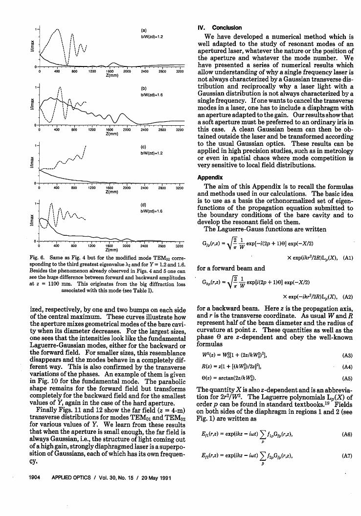
Fig. 6. Same as Fig. 4 but for the modified mode TEM0 2 corre-sponding to the third greatest eigenvalue 2 and for Y = 1.2 and 1.6.Besides the phenomenon already observed in Figs. 4 and 5 one cansee the huge difference between forward and backward amplitudesat z = 1100 mm. This originates from the big diffraction loss
associated with this mode (see Table I).
ized, respectively, by one and two bumps on each sideof the central maximum. These curves illustrate howthe aperture mixes geometrical modes of the bare cavi-ty when its diameter decreases. For the largest sizes,one sees that the intensities look like the fundamentalLaguerre-Gaussian modes, either for the backward orthe forward field. For smaller sizes, this resemblancedisappears and the modes behave in a completely dif-ferent way. This is also confirmed by the transversevariations of the phases. An example of them is givenin Fig. 10 for the fundamental mode. The parabolicshape remains for the forward field but transformscompletely for the backward field and for the smallestvalues of Y again in the case of the hard aperture.
Finally Figs. 11 and 12 show the far field (z = 4-m)transverse distributions for modes TEM01 and TEM0 2for various values of Y. We learn from these resultsthat when the aperture is small enough, the far field isalways Gaussian, i.e., the structure of light coming outof a high gain, strongly diaphragmed laser is a superpo-sition of Gaussians, each of which has its own frequen-cy,
IV. ConclusionWe have developed a numerical method which is
well adapted to the study of resonant modes of anapertured laser, whatever the nature or the position ofthe aperture and whatever the mode number. Wehave presented a series of numerical results whichallow understanding of why a single frequency laser isnot always characterized by a Gaussian transverse dis-tribution and reciprocally why a laser light with aGaussian distribution is not always characterized by asingle frequency. If one wants to cancel the transversemodes in a laser, one has to include a diaphragm withan aperture adapted to the gain. Our results show thata soft aperture must be preferred to an ordinary iris inthis case. A clean Gaussian beam can then be ob-tained outside the laser and be transformed accordingto the usual Gaussian optics. These results can beapplied in high precision studies, such as in metrologyor even in spatial chaos where mode competition isvery sensitive to local field distributions.
AppendixThe aim of this Appendix is to recall the formulas
and methods used in our calculations. The basic ideais to use as a basis the orthonormalized set of eigen-functions of the propagation equation submitted tothe boundary conditions of the bare cavity and todevelop the resonant field on them.
The Laguerre-Gauss functions are written
Gf,(r,z) = 2 exp[-i(2p + 1)0] exp(-X/2)
X exp(ikr 2/2R)L (X), (Al)
for a forward beam and
Gbp(r,z) = ir Wexp[i(2p + 1)0] exp(-X/2)
X exp(-ikr2 2R)Lp(X), (A2)
for a backward beam. Here z is the propagation axis,and r is the transverse coordinate. As usual W and Rrepresent half of the beam diameter and the radius ofcurvature at point z. These quantities as well as thephase are z-dependent and obey the well-knownformulas
W2(z) = W2[l + (2z/kW2)2 ],
R(z) = z4l + [(kWV)/2z] 2 j,
O(z) = arctan(2z/kWo).
(A3)
(A4)
(A5)
The quantity X is also z-dependent and is an abbrevia-tion for 2r 2/W 2. The Laguerre polynomials L(X) oforder p can be found in standard textbooks.'9 Fieldson both sides of the diaphragm in regions 1 and 2 (seeFig. 1) are written as
i . . .a,0 . I I | . . .12 I . . .166 . . .2060 400 800 1 200 1 600 2000Z(mm)
- ... l - .. - -x -----
.
I l/Imax
Y=1.0 (c)
-1.5 -1.0
Fig. 7. Transverse distribution of intensities forthe TEMoo mode for different apertures at z = 750mm inside the cavity. [This point corresponds tothe bump at 750 mm for the backward beam in Fig.4(a).] Here and in the following figures, curves onthe right (left) are drawn for the soft (hard) aper-ture. Hard diffraction [(a) and (b)] makes theforward beam remain Gaussian, while the back-ward beam becomes more and more perturbedwhen the diameter of the aperture decreases. Softdiffraction [(c) or (d)] preserves the transverse
Gaussian character.
(b) Y=1.6 (d)
1.5 -1.5 -1.0 -0.5
b/W(zd)=1.0
17-
1) /I.I
I
II
i/Imax
' b/W(z
..-
1.5 -1.5 -1.0 0.5 0.0 0.5r(mm)
b/W(zd)=1 .4 (e)
I/Imax
b/W(zd)=1 .4
1.0 1.5
(C)'
Fig. 8. Same as Fig. 7 for the modified modeTEM0 1, (c) and (f) display a profile analogous to theusual nonperturbed first transverse mode with abump on each side of the central maximum. Thischaracteristic bump is lost when the aperture is
Fig. 9. Same as Fig. 7 for the modified modeTEM 02, (c) and (f) display a profile analogous to theusual TEM0 2 transverse mode with two bumps oneach side of the central maximum but this time forY= bW(zd) = 2.2. As expected one needs a biggeraperture to recover the fundamental profile for
higher-order modes.
Fig. 10. Transverse phase distribution at z = 750mm for the fundamental mode and for various val-ues of the diameter of the aperture. This phaseremains parabolic for the forward beam. It be-comes strongly modified for the backward beamwhen the diameter of the aperture decreases in the
Fig. 11. Transverse intensity distributions for themodified TEMoi mode in the far field region out-side the cavity (z = 4000 mm) and for variousdiameters of the aperture. Two important conclu-sions are drawn: for large apertures one recoversthe usual nonperturbed profiles [especially Fig.10(d)], while for small diaphragms one obtains aquasi-Gaussian structure [(a) and (e)]. Here theratio Y = 1.8 is not big enough to recover the pure
TEM01 profile in (h).
(c)
VImax
b/W(zd)=1 .6
I - | I I I.3 -2 -1 0 1 2 3
r(mm)
I/lmax
(d) b/W(zd)=1.8--Z \ - f~~~~~~~~~~~
I 0 i . I l
-3 -2 -1
Ebl(r,z) = exp(-ikz - iwt) E bpGbp(rz), (A8)p
Eb(r,z) = exp(-ikz - it) E b2pGbp(rz), (A9)
p
where subscripts f and b stand for forward and back-ward fields and 1 and 2 for the region. The aim of thecomputation is to find the (z-independent) coeffi-cientsf1p,f2 p, b1p, and b2p of the expansion of the fieldson the basis functions (Al) and (A2). Since thesefunctions are solutions of the propagation equation,'the linear combinations (A6)-(A9) also representphysical propagating fields.
0r(mm)
1 2 3
(g)
(h)
-3 -2
b/W(zd)=1 .6
b/W(zd)=1 .8
r(mm)2 3
To find the matrix M which represents the round-trip operator one has to relate the different coeffi-cients, i.e., express, for example, f2p, bp, and b2 interms of fip. Using the Kirchhoff condition at theaperture location z = zd, one relates the fip and the f2p.
link backward coefficients on both sides of the aper-ture:
blq = E b2p exp[-2iOb(q - p)]Cpq. (A15)
p
Now backward and forward fields are related to eachother by reflection. On the concave mirror at z = d onehas
E2b(r,d) = RBE2f(r,d). (A16)
If one uses the relation
Gfp(r,d) = Gbp(r,d) exp[-2i(2p + 1)0d], (A17)
one obtains
> b2pGbp(r,d) = RB E3 f2p exp[-2i(2p + l)0d]P P
X exp(2ikd)Gbp(r,d). (A18)
Here Od is the value of e(z) at z = d. One then obtains
b2p = RBf2p exp[-2i(2p + 1)0d] exp(2ikd). (A19)
Now one can write
b2m = RB exp(-2iOd + 2ikd) exp[2im(Ob - 20d)]
are also complex; they represent losses and phase vari-ations caused by diffraction.
To find the first eigenvector (i.e., corresponding tothe lowest losses) one iterates Eq. (2) [or Eq. (A24)]starting from the fundamental Gaussian mode of thenondiaphragmed cavity [i.e., with the vector(l,0,0,0,...)]. If one takes the precaution to renorma-lize the vector after each iteration (in order not to fallinto the computer noise), one quickly finds the eigen-vector V,, i.e., the coefficients f 1p(i), so that
f1p(i)pf(i - 1) = xi, (A26)
where i is the number of iterations, and X, is just theeigenvalue. It is complex and independent of p.
To obtain the second eigenvector V2 correspondingto the second greatest eigenvalue X2 one builds the newmatrix
M1 = MAl V 1V. (A27)
The algorithm of the iterated power is appliedagain onto M1, starting this time with the vector(0,l,0,0,0,...). One then obtains the perturbedTEMo1 mode with its eigenvalue X2 and components onthe basis of Eq. (Al) or (A2). The TEM0 2 mode isobtained in the same way through the matrix M2:
M2 = M1 - XY2VV2 (A28)
X3 [fip exp(-2ip0b)Cpm]. (A20)
This leads to the relationship between blq and fip:
blq = RB exp(- 2iOd + 2ikd) >3 {fp exp(-2ipeb)p,m
X exp[2im(Ob - 20d)] exp[2i(m - q)0blCpmCmqj. (A21)
Reflection on the plane mirror gives
RAEbl(r,O) = Efl(r,O) or fp = RAblp. (A22)
Finally, after a round trip in the cavity, we obtain
fiq = RARB exp(-2
iOd + 2ikd) > flp exp(-2ipeb)
p,m
X exp[2im(Ob - 20d)I exp[2i(m - q)Ob]CpmCmqJ. (A23)
This equation can be put in matrix form so that
Iiq = > 4Xpqfp (A24)p
with
.Mpq = RARB expf-2i[Od - kd + (p + q)eb]}
X > exp[4im(eb - ed)ICpmCmqI. (A25)
The round-trip operator M is represented by the ma-trix whose elements are /pq. The eigenvectors of thismatrix represent the modes of the apertured cavityand are characterized by the (infinite) series of thecomplex numbers fiq. The corresponding eigenvalues
References1. A. G. Fox and T. Li, "Resonant Modes in a Maser Interferome-
ter," Bell Syst. Tech. J. 40, 453-488 (1961).2. T. Li, "Mode Selection in an Aperture-Limited Concentric Ma-
ser Interferometer," Bell Syst. Tech. J. 42, 2609-2620 (1963).3. A. G. Fox and T. Li, "Modes in a Maser Interferometer with
Curved and Tilted Mirrors," Proc. IEEE 51, 80-89 (1963).4. T. Li, "Diffraction Loss and Selection of Modes in Maser Reso-
nators with Circular Mirrors," Bell Syst. Tech. J. 44, 917-932(1965).
5. M. Piche, P. Lavigne, F. Martin, and P. A. Belanger, "Modes ofResonators with Internal Apertures," Appl. Opt. 22, 1999-2006(1983) and references therein.
6. B. Lissak and S. Ruschin, "Transverse Pattern Modifications ina Stable Apertured Laser Resonator," Appl. Opt. 29, 767-771(1990).
7. A. G. Fox and T. Li, "Computation of Resonator Modes by theMethod of Resonance Excitation," IEEE J. Quantum Electron.QE4, 460-465 (1968).
8. H. Ogura, Y. Yoshida, and I. Iwamoto, "Excitation of Fabry-Perot Resonator-I," J. Phys. Soc. Jpn. 22, 1421-1433 (1967).
9. H. Ogura, Y. Yoshida, and J. Ikenoue, "Excitation of Fabry-Perot Resonator-II. Free Oscillation," J. Phys. Soc. Jpn. 22,1434-1445 (1967).
10. L. A. Vainshtein, "Open Resonators for Lasers," Zh. Eksp. Teor.Fiz. 44, 1050-1060 (1963) [Sov. Phys. JETP 17,709-719 (1963)].
11. V. F. Boitsov and T. A. Murina, "Field and Loss Properties in aThree-Mirror Ring Optical Resonator with a Gaussian Diaph-ragm," Opt. Spektrosk. 34, 572-575 (1973) [Opt. Spectrosc.USSR 34, 327-330 (1973)].
12. L. W. Casperson and S. D. Lunnam, "Gaussian Modes in HighLoss Laser Resonators," Appl. Opt. 14, 1193-1199 (1975).
13. G. Stephan and M. Trumper, "Inhomogeneity Effects in a GasLaser," Phys. Rev. A 28, 2344-2362 (1983).
14. K. Ait-Ameur and H. Ladjouze, "Fundamental Mode Distribu-tion in a Diaphragmed Cavity," J. Phys. D 21,1566-1571 (1988).
15. A. Kellou and G. Stephan, "Etude du Champ Proche d'un LaserDiaphragm6," Appl. Opt. 26, 76-90 (1987).
16. K. Arbenz and A. Wohlhauser, "Analyse numerique," PressesPolytech. Romandes 46-49 (1980).
17. H. J. Caulfield, D. S. Dvore, J. W. Goodman, and W. T. Rhodes,"Eigenvector Determination by Noncoherent Optical Meth-ods," Appl. Opt. 20, 2263-2265 (1981).
18. G. Otis, J.-L. Lachambre, and P. Lavigne, "Focusing of LaserBeams by a Sequence of Irises," Appl. Opt. 18, 875-883 (1979).
19. G. Arfken, Mathematical Methods for Physicists (Academic,New York, 1973), pp. 616-622.