Transverse motion as a source of noise and reduced correlation of the Doppler phase shift in...

Transverse motion as a source of noise and reduced correlation of the Doppler phase shift

in spectral domain OCT

Julia Walther and Edmund Koch*

Department of Clinical Sensoring and Monitoring, Medical Faculty Carl Gustav Carus, University of Technology Dresden, Fetscherstrasse 74, 01307 Dresden, Germany

*[email protected]

Abstract: Recently, a new phase-resolved Doppler model was presented for spectral domain optical coherence tomography (SD OCT) showing that the linear relation between the axial velocity component of the obliquely moving sample and the phase difference of consecutive A-Scans does not hold true in the presence of a transverse velocity component which is neglected in the widely-used classic Doppler analysis. Besides taking note of the new non-proportional relationship of phase shift and oblique sample motion, it is essential to consider the correlation of the phase shift and its specific characteristic at certain Doppler angles for designing Doppler experiments with SD OCT. A correlation quotient is introduced to quantify the correlation of the backscattering signal in consecutive A-Scans as a function of the oblique sample motion. It was found that at certain velocities and Doppler angles no correlation of the phases of sequential A-Scans exists, even though the signal does not vanish. To indicate how the noise of the Doppler phase shift behaves for oblique movement, the standard deviation is determined as a function of the correlation quotient and the number of complex Doppler data averaged. The detailed theoretical model is validated by using a flow phantom model consisting of a 1% Intralipid flow through a 310 µm capillary. Finally, a short discussion of the presented results and the consequence for performing Doppler experiments is given.

©2009 Optical Society of America

OCIS codes: (110.4500) Optical coherence tomography; (120.5050) Phase measurement; (110.4153) Motion estimation and optical flow; (280.2490) Flow diagnosis.

References and links

1. D. Huang, E. A. Swanson, C. P. Lin, J. S. Schuman, W. G. Stinson, W. Chang, M. R. Hee, T. Flotte, K. Gregory, C. A. Puliafito, and J. G. Fujimoto, “Optical coherence tomography,” Science 254(5035), 1178–1181 (1991).

2. Y. T. Pan, Z. L. Wu, Z. J. Yuan, Z. G. Wang, and C. W. Du, “Subcellular imaging of epithelium with time-lapse optical coherence tomography,” J. Biomed. Opt. 12(5), 050504 (2007).

3. W. Drexler, U. Morgner, F. X. Kärtner, C. Pitris, S. A. Boppart, X. D. Li, E. P. Ippen, and J. G. Fujimoto, “In vivo ultrahigh-resolution optical coherence tomography,” Opt. Lett. 24(17), 1221–1223 (1999).

4. J. F. de Boer, T. E. Milner, M. J. C. van Gemert, and J. S. Nelson, “Two-dimensional birefringence imaging in biological tissue by polarization-sensitive optical coherence tomography,” Opt. Lett. 22(12), 934–936 (1997).

5. M. Pircher, E. Goetzinger, R. Leitgeb, and C. Hitzenberger, “Three dimensional polarization sensitive OCT of human skin in vivo,” Opt. Express 12(14), 3236–3244 (2004).

6. Z. G. Wang, C. S. D. Lee, W. C. Waltzer, J. X. Liu, H. K. Xie, Z. J. Yuan, and Y. T. Pan, “In vivo bladder imaging with microelectromechanical-systems-based endoscopic spectral domain optical coherence tomography,” J. Biomed. Opt. 12(3), 034009 (2007).

7. G. J. Tearney, M. E. Brezinski, B. E. Bouma, S. A. Boppart, C. Pitris, J. F. Southern, and J. G. Fujimoto, “In vivo endoscopic optical biopsy with optical coherence tomography,” Science 276(5321), 2037–2039 (1997).

8. U. Morgner, W. Drexler, F. X. Kärtner, X. D. Li, C. Pitris, E. P. Ippen, and J. G. Fujimoto, “Spectroscopic optical coherence tomography,” Opt. Lett. 25(2), 111–113 (2000).

9. R. Leitgeb, M. Wojtkowski, A. Kowalczyk, C. K. Hitzenberger, M. Sticker, and A. F. Fercher, “Spectral measurement of absorption by spectroscopic frequency-domain optical coherence tomography,” Opt. Lett. 25(11), 820–822 (2000).

10. R. K. Wang, Z. Ma, and S. J. Kirkpatrick, “Tissue Doppler optical coherence elastography for real time strain rate and strain mapping of soft tissue,” Appl. Phys. Lett. 89(14), 144103 (2006).

#116704 - $15.00 USD Received 3 Sep 2009; revised 12 Oct 2009; accepted 14 Oct 2009; published 15 Oct 2009

(C) 2009 OSA 26 October 2009 / Vol. 17, No. 22 / OPTICS EXPRESS 19698

11. S. J. Kirkpatrick, R. K. Wang, and D. D. Duncan, “OCT-based elastography for large and small deformations,” Opt. Express 14(24), 11585–11597 (2006).

12. X. J. Wang, T. E. Milner, and J. S. Nelson, “Characterization of fluid flow velocity by optical Doppler tomography,” Opt. Lett. 20(11), 1337–1339 (1995).

13. Z. Chen, T. E. Milner, S. Srinivas, X. Wang, A. Malekafzali, M. J. C. van Gemert, and J. S. Nelson, “Noninvasive imaging of in vivo blood flow velocity using optical Doppler tomography,” Opt. Lett. 22(14), 1119–1121 (1997).

14. Z. Chen, T. E. Milner, D. Dave, and J. S. Nelson, “Optical Doppler tomographic imaging of fluid flow velocity in highly scattering media,” Opt. Lett. 22(1), 64–66 (1997).

15. J. A. Izatt, M. D. Kulkarni, S. Yazdanfar, J. K. Barton, and A. J. Welch, “In vivo bidirectional color Doppler flow imaging of picoliter blood volumes using optical coherence tomography,” Opt. Lett. 22(18), 1439–1441 (1997).

16. Z. Xu, L. Carrion, and R. Maciejko, “A zero-crossing detection method applied to Doppler OCT,” Opt. Express 16(7), 4394–4412 (2008).

17. H. Ren, K. M. Brecke, Z. Ding, Y. Zhao, J. S. Nelson, and Z. Chen, “Imaging and quantifying transverse flow velocity with the Doppler bandwidth in a phase-resolved functional optical coherence tomography,” Opt. Lett. 27(6), 409–411 (2002).

18. B. White, M. Pierce, N. Nassif, B. Cense, B. Park, G. Tearney, B. Bouma, T. Chen, and J. de Boer, “In vivo dynamic human retinal blood flow imaging using ultra-high-speed spectral domain optical coherence tomography,” Opt. Express 11(25), 3490–3497 (2003).

19. R. Leitgeb, L. Schmetterer, W. Drexler, A. Fercher, R. Zawadzki, and T. Bajraszewski, “Real-time assessment of retinal blood flow with ultrafast acquisition by color Doppler Fourier domain optical coherence tomography,” Opt. Express 11(23), 3116–3121 (2003).

20. L. Wang, Y. Wang, S. Guo, J. Zhang, M. Bachman, G. P. Li, and Z. Chen, “Frequency domain phase-resolved optical Doppler and Doppler variance tomography,” Opt. Commun. 242(4-6), 345–350 (2004).

21. Y. Wang, B. A. Bower, J. A. Izatt, O. Tan, and D. Huang, “In vivo total retinal blood flow measurement by Fourier domain Doppler optical coherence tomography,” J. Biomed. Opt. 12(4), 041215 (2007).

22. B. A. Bower, M. Zhao, R. J. Zawadzki, and J. A. Izatt, “Real-time spectral domain Doppler optical coherence tomography and investigation of human retinal vessel autoregulation,” J. Biomed. Opt. 12(4), 041214 (2007).

23. H. Wehbe, M. Ruggeri, S. Jiao, G. Gregori, C. A. Puliafito, and W. Zhao, “Automatic retinal blood flow calculation using spectral domain optical coherence tomography,” Opt. Express 15(23), 15193–15206 (2007).

24. Y. Wang, A. Fawzi, O. Tan, J. Gil-Flamer, and D. Huang, “Retinal blood flow detection in diabetic patients by Doppler Fourier domain optical coherence tomography,” Opt. Express 17(5), 4061–4073 (2009).

25. T. Schmoll, C. Kolbitsch, and R. A. Leitgeb, “Ultra-high-speed volumetric tomography of human retinal blood flow,” Opt. Express 17(5), 4166–4176 (2009).

26. A. Mariampillai, B. A. Standish, N. R. Munce, C. Randall, G. Liu, J. Y. Jiang, A. E. Cable, I. A. Vitkin, and V. X. D. Yang, “Doppler optical cardiogram gated 2D color flow imaging at 1000 fps and 4D in vivo visualization of embryonic heart at 45 fps on a swept source OCT system,” Opt. Express 15(4), 1627–1638 (2007).

27. B. Vakoc, S. Yun, J. de Boer, G. Tearney, and B. Bouma, “Phase-resolved optical frequency domain imaging,” Opt. Express 13(14), 5483–5493 (2005).

28. S. H. Yun, G. Tearney, J. de Boer, and B. Bouma, “Motion artifacts in optical coherence tomography with frequency-domain ranging,” Opt. Express 12(13), 2977–2998 (2004).

29. R. Leitgeb, C. Hitzenberger, and A. Fercher, “Performance of fourier domain vs. time domain optical coherence tomography,” Opt. Express 11(8), 889–894 (2003).

30. M. Choma, M. Sarunic, C. Yang, and J. Izatt, “Sensitivity advantage of swept source and Fourier domain optical coherence tomography,” Opt. Express 11(18), 2183–2189 (2003).

31. M. Szkulmowski, A. Szkulmowska, T. Bajraszewski, A. Kowalczyk, and M. Wojtkowski, “Flow velocity estimation using joint Spectral and Time domain Optical Coherence Tomography,” Opt. Express 16(9), 6008–6025 (2008).

32. A. Szkulmowska, M. Szkulmowski, D. Szlag, A. Kowalczyk, and M. Wojtkowski, “Three-dimensional quantitative imaging of retinal and choroidal blood flow velocity using joint Spectral and Time domain Optical Coherence Tomography,” Opt. Express 17(13), 10584–10598 (2009).

33. R. K. Wang, S. L. Jacques, Z. Ma, S. Hurst, S. R. Hanson, and A. Gruber, “Three dimensional optical angiography,” Opt. Express 15(7), 4083–4097 (2007).

34. Y. K. Tao, A. M. Davis, and J. A. Izatt, “Single-pass volumetric bidirectional blood flow imaging spectral domain optical coherence tomography using a modified Hilbert transform,” Opt. Express 16(16), 12350–12361 (2008).

35. Y. K. Tao, K. M. Kennedy, and J. A. Izatt, “Velocity-resolved 3D retinal microvessel imaging using single-pass flow imaging spectral domain optical coherence tomography,” Opt. Express 17(5), 4177–4188 (2009).

36. A. H. Bachmann, M. L. Villiger, C. Blatter, T. Lasser, and R. A. Leitgeb, “Resonant Doppler flow imaging and optical vivisection of retinal blood vessels,” Opt. Express 15(2), 408–422 (2007).

37. V. Yang, M. Gordon, B. Qi, J. Pekar, S. Lo, E. Seng-Yue, A. Mok, B. Wilson, and I. Vitkin, “High speed, wide velocity dynamic range Doppler optical coherence tomography (Part I): System design, signal processing, and performance,” Opt. Express 11(7), 794–809 (2003).

38. B. H. Park, M. C. Pierce, B. Cense, S. H. Yun, M. Mujat, G. J. Tearney, B. E. Bouma, and J. F. de Boer, “Real-time fiber-based multi-functional spectral-domain optical coherence tomography at 1.3 microm,” Opt. Express 13(11), 3931–3944 (2005).

39. B. J. Vakoc, G. J. Tearney, and B. E. Bouma, “Statistical properties of phase-decorrelation in phase-resolved Doppler optical coherence tomography,” IEEE Trans. Med. Imaging 28(6), 814–821 (2009).



40. E. Koch, J. Walther, and M. Cuevas, “Limits of Fourier domain Doppler-OCT at high velocities,” Sensors and Actuators A, doi:10.1016/j.sna.2009.01.022.

41. G. Lamouche, M. L. Dufour, B. Gauthier, and J. Monchalin, “Gouy phase anomaly in optical coherence tomography,” Opt. Commun. 239(4-6), 297–301 (2004).

42. J. Walther, A. Krüger, M. Cuevas, and E. Koch, “Effects of axial, transverse and oblique sample motion in FD OCT in systems with global or rolling shutter line detector,” J. Opt. Soc. Am. A 25(11), 2791–2802 (2008).

43. S. Meißner, G. Muller, J. Walther, A. Krüger, M. Cuevas, B. Eichhorn, U. Ravens, H. Morawietz, and E. Koch, “Investigation of murine Vasodynamics by Fourier Domain Optical Coherence Tomography,” Proc. SPIE 6627, 66270D (2007).

44. J. Walther, G. Muller, H. Morawietz, and E. Koch, “Analysis of in vitro and in vivo bidirectional flow velocities by phase-resolved Doppler Fourier-domain OCT,” Sens. Actuators A .

45. A. Szkulmowska, M. Szkulmowski, A. Kowalczyk, and M. Wojtkowski, “Phase-resolved Doppler optical coherence tomography--limitations and improvements,” Opt. Lett. 33(13), 1425–1427 (2008).

46. J. Walther, and E. Koch, “Flow measurement by using the signal decrease of moving scatterers in spatially encoded Fourier domain optical coherence tomography,” Proc. SPIE 7168, 71681S (2009).

47. B. Karamata, K. Hassler, M. Laubscher, and T. Lasser, “Speckle statistics in optical coherence tomography,” J. Opt. Soc. Am. A 22(4), 593–596 (2005).

48. J. W. You, T. C. Chen, M. Mujat, B. H. Park, and J. F. de Boer, “Pulsed illumination spectral-domain optical coherence tomography for human retinal imaging,” Opt. Express 14(15), 6739–6748 (2006).

1. Introduction

Optical coherence tomography (OCT) [1] is a non-invasive, contactless imaging modality which provides cross-sectional images of highly scattering samples such as biological tissue at a resolution of a few micrometer. Further technological developments were adapted to this imaging technique to permit e.g. ultrahigh-resolution OCT (UHROCT) to characterize cellular microstructures [2,3], polarization-sensitive OCT for in vivo investigation of the birefringence properties of human tissue [4,5] and endoscopic OCT allowing in vivo imaging of internal organs [6,7]. Furthermore, imaging advances have been emerged for the visualization and quantification of physiological parameters of biological tissue such as metabolism [8,9], elastography [10,11] and blood circulation [12–15]. To realize the latter, Doppler OCT or optical Doppler tomography (ODT) was explored to measure velocities, especially blood flow velocities [12–15]. In time domain OCT (TD OCT), the Doppler frequency shift in the interference fringe intensity modulation is used to calculate the axial velocity component of the flow [16]. To quantify the transverse component of the flow velocity the Doppler bandwidth was considered [17]. In Fourier domain OCT (FD OCT), the simplest and most prevalent way to measure flow velocities is called phase-resolved Doppler OCT. This technique is based on the linear relation of the phase change of sequentially acquired interference signals and the axial sample velocity [18–27]. Because of the high phase stability of spectral domain OCT (SD OCT) systems, as an advantage over optical frequency domain imaging (OFDI) [28], and the fact of a high signal-to-noise ratio (SNR) compared to TD OCT [29,30], Doppler flow imaging is often performed in combination with SD OCT [18–25].

Different advances in Doppler FD OCT have recently been suggested for qualitative and quantitative flow measurements. For instance, a method using a two dimensional Fourier transformation of the spectral data called joint Spectral and Time domain Optical coherence tomography (STdOCT) has been proposed to measure velocities of scattering parts with a low SNR [31]. Most recently, this technique has presented its potential for 3D retinal and choroidal imaging in the human eye [32]. Another technique for blood flow mapping is the 3D optical angiography (OAG) [33] which is based on the spatial frequency modulation technique by imposing a constant Doppler frequency shift to separate the dynamic flow signal from the static one by a transverse Hilbert transform. Here, R. K. Wang’s group sets the velocity threshold by moving the reference mirror. In contrast, an improvement on the 3D optical angiography was demonstrated by Y. K. Tao et al. using a modified Hilbert transform algorithm for 3D flow detection without the use of spatial frequency modulation. This technique called single-pass volumetric bidirectional blood flow imaging (SPFI) [34] was enhanced by a moving spatial frequency window to achieve a velocity-resolved SPFI of several volumes within one 3D scan [35]. Similar to the 3D OAG by R. K. Wang, resonant Doppler flow imaging also generates a variable phase delay in the reference arm but uses an electro-optic phase modulator [36]. This method relies only on the amplitude of the scattering



signal and overcomes the signal power decrease due to sample motion [28]. The sample velocity is calculated by comparing the interference signal for the reference arm moving forward or backward to the signal when the reference arm is at rest. Despite of the multifaceted enhancements in flow velocity detection by FD OCT, the most common and straightforward method for quantitative flow measurements with SD OCT is to determine the axial velocity component vz by using its proportionality to the calculated phase shift ∆φ between adjacent A-Scans [18–25]:

0

4

A Scan

z

fv

n

ϕ λπ

−∆ ⋅ ⋅=

⋅ (1)

where λ0 is the center wavelength of the OCT system, fA-Scan the A-Scan frequency and n the refractive index of the medium. With known Doppler angle, the absolute sample velocity v can be calculated. In a laminar flow which can be assumed for flowing blood in most cases, phase shifts of more than π can be identified uniquely by phase unwrapping techniques [37].

In SD OCT, the prevalent classic Doppler model acts on the assumption that the phase shift between adjacent A-Scans is proportional to the axial velocity. But at least for transverse velocity components per A-Scan integration time TInt larger than the sample beam diameter, one would expect deviations from the classic Doppler model. The effect of the sample beam movement on the standard deviation of the phase shift was investigated by B. H. Park et al. [38]. In this study, the continuous movement of the beam and the sample during the integration time was neglected and the axial velocity component was not taken into account. The continuation of this question was given by B. J. Vakoc et al. [39] investigating the decorrelation noise due to the sample beam displacement between two consecutive measurements for an OFDI system. A new phase-dependent Doppler model for SD OCT was presented recently by our group which does not ignore the transverse component of the oblique sample movement and its influence on the resulting Doppler phase shift [40]. In this study, a correlation quotient (CQ) is defined as an essential improvement of the new Doppler model which describes the correlation of the backscattering signal in consecutive A-Scans as a function of the oblique sample motion. Furthermore, the noise of the Doppler phase shift is analyzed as a function of CQ and the number of samples for averaging. To validate the correlation quotient of the new Doppler model and to ascertain the standard deviation of the phase shift as a function of CQ, in vitro experiments were carried out using a capillary model with a 1% Intralipid emulsion.

2. Theory of the New Phase-dependent Doppler Model

The effect of oblique sample motion on the relation between phase shift and sample velocity has been described in detail in a previous study [40]. For the derivation of the introduced correlation quotient in Section 3, the revised theoretical analysis of the new phase-dependent Doppler model is briefly summarized in this section.

The oblique sample movement consists of an axial component ∆z = vz⋅TInt and a transverse

one ∆x = vx⋅TInt where vz and vx are the axial and transverse velocity components and TInt is the integration time of the CCD line detector. For the theoretical consideration, the blurring of the Gaussian beam outside the focal plane as well as the Gouy phase shift are neglected [41]. For the general description of the phase shift, dimensionless coordinates are defined for the displacements δx and δz as well as for the time t’ where w0 corresponds to the beam width (FWHM) of the Gaussian sample beam, λ0 is the center wavelength of the OCT system and n represents the refractive index of the investigated medium.

00

, , '

2Int

x z tx z t

w Tn

δ δλ

∆ ∆= = = (2, 3, 4)

The integration time for each A-Scan has the length δt’ = 1. Following the argumentation of Yun et al. [28] given for a small spectral bandwidth, the integration of the photocurrent



gives a signal that is proportional to Eq. (5). The variables T1 und T2 are the borders of the time interval TInt, xm is the normalized coordinate in x-direction at t’ = 0 and am is the complex amplitude of a scatterer m combining the amplitude and the phase of the backscattered light. The sum in front of the integral corresponds to the summation of all individual backscattered signals am of multiple continuously moving scatterers with identical velocity but different positions xm.

( )

22

1

4ln(2) '2 '

1 2( , , , ) 'm

T

x x ti z t

m

m T

N T T x z a e e dtδπ δδ δ − −= ⋅∑ ∫ (5)

The phase shift ∆φ between two adjacent A-Scans is calculated as presented in Eqs. (6) and (7). Accordingly, ∆φ corresponds to the argument of the product of the complex amplitude N of the first A-Scan and the complex conjugate value N

* of the second A-Scan

[23]. For simplicity, two consecutive A-Scans in the time intervals [-1,0] and [0,1] are considered.

( )( )arg ,corC x zϕ δ δ∆ = (6)

( ) ( ) ( )*, 1,0, , 0,1, ,

corC x z N x z N x zδ δ δ δ δ δ= − ⋅ (7)

Only for the case of a transverse velocity vx of zero (δx = 0), the integral resulting from Eq. (6) can be solved analytically, leading to the linear relation between ∆φ and vz in accordance to Eq. (1) [40]. Unfortunately, no analytical solution of the integral can be given for finite δx [42]. In this case, the product of sums in Eq. (7) can be expressed as:

( ) ( ) ( )

( ) ( )

*

*

,

, 1,0, , , 0,1, , ,

1,0, , , 0,1, , , .

cor

m

m km k

C x z N x z m N x z m

N x z m N x z k

δ δ δ δ δ δ

δ δ δ δ

≠

= − ⋅ +

− ⋅

∑

∑ (8)

To explain the different parts in Eq. (8), the case of a sample velocity of zero is considered. In this case, N(T1,T2,δx,δz) = N(T1,T2,0,0) does not depend on time and corresponds to the complex result of the Fourier transform of the integrated photocurrent. The signal from different scatterers adds up to the total signal N. The product

N(T1,T2,δx,δz)⋅N*(T1,T2,δx,δz) corresponds to the intensity caused by the interference from the

different scatterers which consists of the sum of squares of each signal, the first part in Eq. (8), and the interference term between all the pairs (m and k) of scatterers, which relates to the second part. While the mean value of the second part is zero over all possible combinations of scatterers, the rms-value of both sums is similar leading to the huge span of intensities (speckle noise). For finite sample velocities, as in the case of zero velocity, the average of the second term will disappear due to the arbitrary phases. As a result, the averaged value of Ccor (Eq. (8)) can be described by Eq. (9).

( ) ( ) ( )*, 1,0, , , 0,1, , ,cor

m

C x z N x z m N x z mδ δ δ δ δ δ= − ⋅∑ (9)

This average can be calculated by replacing the sum with the integral over all values of xm. As we are only interested in relative values, we normalize the integral to the average value at zero velocity.

( )( )

*

*

( 1,0, , , ) (0,1, , , ),

0,0( 1,0,0,0, ) (0,1,0,0, )

m m m

cor

corm m m

N x z x N x z x dxC x z

CN x N x dx

δ δ δ δδ δ

∞

−∞∞

−∞

− ⋅

=

− ⋅

∫

∫ (10)

Due to this normalization, the absolute value of |am|2 cancels down. Consequently, the

following integral in Eq. (11) has to be solved:



( ) ( ) ln(4) *, 0,0 2 ( 1,0, , , ) (0,1, , , )cor cor m m mC x z C N x z x N x z x dxπδ δ δ δ δ δ

∞

−∞

= ⋅ − ⋅∫ (11)

where the value 1 2

( , , , , )m

N T T x z xδ δ is defined by Eq. (12) and the factor in front of the

integral is the result of the integration over all values of xm for zero velocity.

( )

22

1

4 ln(2) '2 '

1 2( , , , , ) 'm

T

x x ti z t

m

T

N T T x z x e e dtδπ δδ δ − −= ∫ (12)

The integral in Eq. (11) is numerically solved by global adaptive integration strategies using Mathematica

® 6.0 (Wolfram Research, Inc.). The double integral in Eq. (11) can be

evaluated for any δx and δz without any further transformation. The resulting phase shift as a function of δx and δz is shown by a contour plot in Fig. 1a. The data points for the contour plot were selected on an adaptive grid with smaller step sizes in the regions of large changes of the function. The computation of the plot takes several hours on a normal PC.

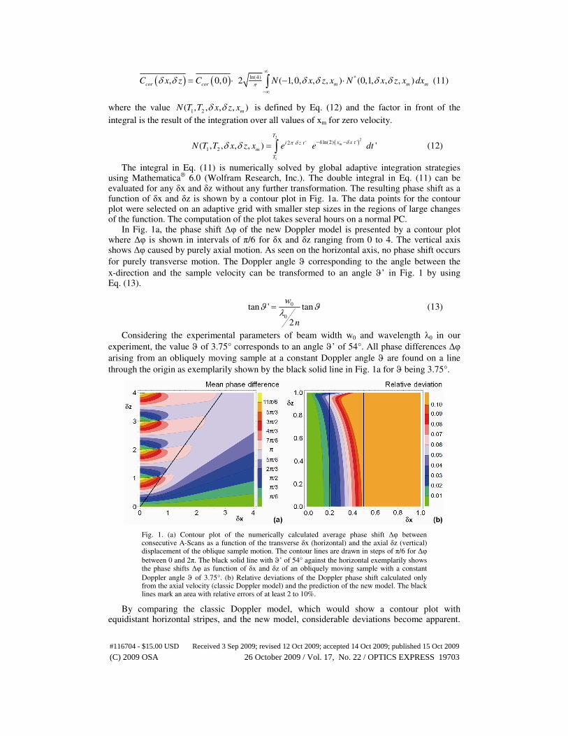
In Fig. 1a, the phase shift ∆φ of the new Doppler model is presented by a contour plot where ∆φ is shown in intervals of π/6 for δx and δz ranging from 0 to 4. The vertical axis shows ∆φ caused by purely axial motion. As seen on the horizontal axis, no phase shift occurs

for purely transverse motion. The Doppler angle ϑ corresponding to the angle between the

x-direction and the sample velocity can be transformed to an angle ϑ’ in Fig. 1 by using Eq. (13).

0

0

tan ' tan

2

w

n

ϑ ϑλ

= (13)

Considering the experimental parameters of beam width w0 and wavelength λ0 in our

experiment, the value ϑ of 3.75° corresponds to an angle ϑ’ of 54°. All phase differences ∆φ

arising from an obliquely moving sample at a constant Doppler angle ϑ are found on a line

through the origin as exemplarily shown by the black solid line in Fig. 1a for ϑ being 3.75°.

Fig. 1. (a) Contour plot of the numerically calculated average phase shift ∆φ between consecutive A-Scans as a function of the transverse δx (horizontal) and the axial δz (vertical) displacement of the oblique sample motion. The contour lines are drawn in steps of π/6 for ∆φ

between 0 and 2π. The black solid line with ϑ’ of 54° against the horizontal exemplarily shows the phase shifts ∆φ as function of δx and δz of an obliquely moving sample with a constant

Doppler angle ϑ of 3.75°. (b) Relative deviations of the Doppler phase shift calculated only from the axial velocity (classic Doppler model) and the prediction of the new model. The black lines mark an area with relative errors of at least 2 to 10%.

By comparing the classic Doppler model, which would show a contour plot with equidistant horizontal stripes, and the new model, considerable deviations become apparent.



The resulting relative deviations of the phase shift for δx and δz smaller than one are presented in Fig. 1b. The relative error is shown in steps of 1% up to 10%. The orange color shows areas with more than 10% deviation. The drawn black vertical lines at δx = 0.2 and δx = 0.5 mark regions where the deviations are at least 2 or 10%, respectively. Note that a transverse scanning might cause these errors in spite of purely axial sample movement.

3. Correlation and Noise of the Doppler Phase Shift

3.1 The Correlation Quotient

The presented model gives an explanation for “noise” in the Doppler signal which is independent from experimental parameters like stability of the optical setup, detector and shot noise. Due to different phase shifts caused by particles at different positions in the sample beam, some inherent fluctuations will appear. For this, we consider the absolute value of the product of two consecutive A-Scans which corresponds to the absolute value of Eq. (11) and is defined as the mean correlated signal Icor,mean.

( )( ) ( ) ( )( )*

,, 1,0, , 0,1, ,

cor mean corI abs C x z abs N x z N x zδ δ δ δ δ δ= = − ⋅ (14)

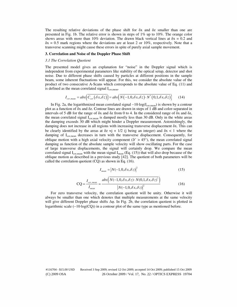
In Fig. 2a, the logarithmized mean correlated signal −10⋅log(Icor,mean) is shown by a contour plot as a function of δx and δz. Contour lines are drawn in steps of 1 dB and color-separated in intervals of 5 dB for the range of δx and δz from 0 to 4. In the considered range of δx and δz, the mean correlated signal Icor,mean is damped mostly less than 30 dB. Only in the white areas the damping exceeds 30 dB which might hinder a Doppler measurement. Astonishingly, the damping does not increase in all regions with increasing transverse displacement δx. This can

be clearly identified by the areas at δz ≈j + 1/2 (j being an integer) and δx < 1 where the damping of Icor,mean decreases in turn with the transverse displacement. Consequently, for

oblique motion with a high axial velocity component (ϑ’ > 45°), the mean correlated signal damping as function of the absolute sample velocity will show oscillating parts. For the case of large transverse displacements, the signal will certainly drop. We compare the mean correlated signal Icor,mean with the mean signal Imean (Eq. (15)) that will also drop because of the oblique motion as described in a previous study [42]. The quotient of both parameters will be called the correlation quotient (CQ) as shown in Eq. (16).

2

( 1,0, , )mean

I N x zδ δ= − (15)

( )*

,

2

( 1,0, , ) (0,1, , )CQ

( 1,0, , )

cor mean

mean

abs N x z N x zI

I N x z

δ δ δ δ

δ δ

− ⋅= =

− (16)

For zero transverse velocity, the correlation quotient will be unity. Otherwise it will always be smaller than one which denotes that multiple measurements at the same velocity will give different Doppler phase shifts ∆φ. In Fig. 2b, the correlation quotient is plotted in

logarithmic scale (−10⋅log(CQ)) in a contour plot of the same type as mentioned before.



Fig. 2. (a) Contour plot showing the damping of the mean correlated signal Icor,mean due to transverse (δx) and axial (δz) displacement. Contour lines are drawn in steps of 1 dB and color values alter in steps of 5 dB. The damping in the white area exceeds 30 dB. (b) Correlation quotient (CQ) due to oblique motion shown by a contour plot as before. The black line with

ϑ' = 54° corresponds to the values of CQ compared with experimental data shown in Fig. 4.

In general, the CQ drops relatively slow with δx. Astonishingly, the quotient becomes zero

at δx ≈0.64 and δz ≈1.06 where all the contour lines of the phase shift meet (cp. Figure 1a). At those points, the measured phase shifts between consecutive A-Scans are totally uncorrelated and randomly distributed. This implies that for scatterers at different transverse positions, the phase shift between adjacent A-Scans has quite different values which average to zero even though a significant backscattering signal exists. Similar points are at slightly higher values of δx (increasing to approximately 0.67) and a little more than integer values of δz. Furthermore,

for ϑ’ > 45°, the damping of the CQ is smaller than 4 dB exempt from the small areas around

δx ≈0.64 and δz ≈j (j being an integer). The reason for this effect was presented in a previous study [42]. For the case of a large axial displacement, only the scatterers located in the sample beam at the start or the end of the integration time TInt contribute to the signal. The

contributions of the scatterers detected in the middle of TInt are decreasing with increasing ϑ until this signal is completely washed out. Consequently, the signal of those scatterers which pass through the sample beam during TInt have only a small influence on the entire signal and

with this on the correlation. In contrast, for ϑ’ < 45°, the contribution of the scatterers seen in the middle part of TInt is significant. Since these scatterers are not present in the subsequent A-Scans at high sample velocities, CQ decreases (cp. Figure 2b). The experimental measurement of CQ will be presented in Section 5.

3.2 The Effect of Finite Spectral Bandwidth

While the new Doppler model with its correlation quotient CQ so far was developed for small spectral bandwidth used in the OCT system, we will consider the effect of a large bandwidth in this section. The effect of purely axial sample movement on the OCT signal was treated in an analytical way in [36]. Deviations for larger bandwidths were mostly seen in the vicinity of velocities that would result in a vanishing signal for monochromatic light. Because in the case of oblique motion there is no analytical solution of the integrals even for monochromatic light, we will not attempt to give an analytical solution for a finite spectral bandwidth.

Because the contour plots presented in Figs. 1 and 2 are shown for normalized displacements δx and δz (cp. Equations (2), (3)), the presented results are valid for any center wavelength λ0 used in the OCT system. Therefore, the effect of a finite spectral bandwidth can be considered by looking at the results of the phase shift ∆φ and the correlation quotient CQ for different center wavelengths λ0. In most cases the beam diameter w0 will change only slightly with λ0, while the axial displacement δz is inversely proportional to λ0 (cp. Equation (3)). Consequently, the phase shift ∆φ and the correlation quotient CQ as functions of the



wavelength can be determined from small, almost vertical lines (δx ≈const.) starting at the

smallest quotient of δzL = 2n⋅∆z/λL and ending at δzS = 2n⋅∆z/λS, where λL and λS are the long and short wavelength limits of the spectral range. As the curves of Icor,mean, Imean and ∆φ are quite smooth in most areas, the influence of a large spectral bandwidth will be small in these areas leading only to a minor broadening of the axial peak shape of the SD OCT signal. In the areas where Icor,mean disappears for monochromatic light, the effect of finite spectral bandwidth will be similar to the effect shown by A. H. Bachmann et al. [36]. Instead of a vanishing signal, the SD OCT signal peak will split into two diverging peaks of small amplitude. Because of the small amplitude and the random character of the signal, the peak splitting will be difficult to observe.

3.3 Tradeoff between Beam Size and Integration Time

For performing Doppler experiments, the parameters spot size w0 and integration time TInt have to be chosen carefully to achieve optimal imaging results. The universal contour plots as shown in Figs. 1 and 2 are applicable for any center wavelength λ0 and beam size w0, independent of TInt. By considering Eq. (13), it can be noted that the larger the spot size w0 is

chosen the larger becomes the angle ϑ’ at constant center wavelength λ0 and Doppler angle ϑ. As a result, the influence of the transverse velocity can be reduced by choosing a larger w0. The disadvantage of this approach is that the transverse resolution of the OCT system decreases which is unfavorable for high resolution morphological and flow imaging of especially small blood vessels. A small quotient of vessel diameter to beam size will certainly reduce the accuracy of blood flow measurement. Additionally, an increase of the spot size results in a decrease of the numerical aperture of the objective of the sample beam and with this in a decrease of the backscattered light collected which in turn causes a reduced intensity signal. The second important parameter for the Doppler measurement is the integration time TInt which represents the limiting factor for the maximum axial velocity component vz measurable without using phase unwrapping techniques (cp. Equation (1)). In order to avoid the observed effects, it is helpful to choose a smaller TInt. But it has to be noted that the smaller TInt is used the more the SNR of the signal decreases and with this the minimum detectable axial velocity vz increases [38]. Consequently, TInt has to be adapted to the region of interest of the phase shift which could possibly be difficult for the quantification of pulsatile flow velocities under in vivo conditions.

4. Experimental Setup

4.1 The SD OCT System and Doppler Analysis

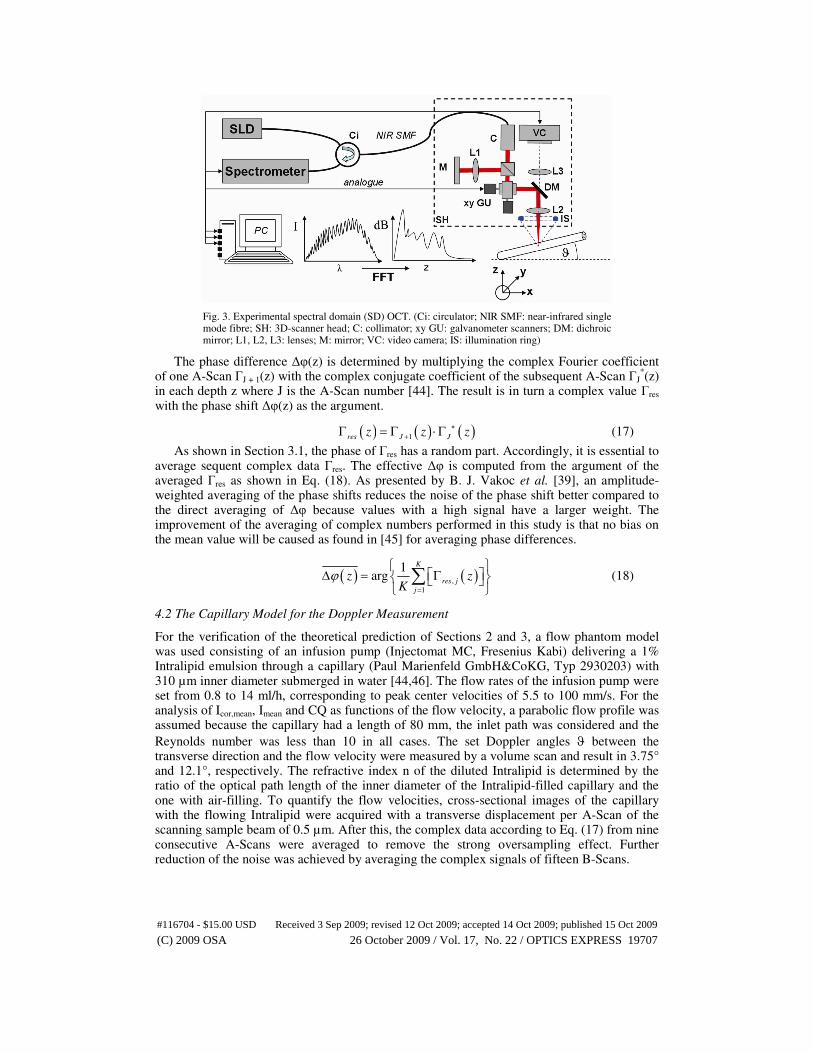
The spectral domain OCT (SD OCT) system used in this study has been described previously [43,44] and is schematically drawn in Fig. 3. The short-coherent light source is a superluminescent diode (SLD 371MP, Superlumdiodes Ltd.) with a center wavelength of λ0 = 840 nm and a full width half maximum of FWHM = 50 nm. Furthermore, the system consists of a directional coupler, a fiber coupled 3D-scanner head with integrated reference arm and a self-developed spectrometer. The sample beam has a measured FWHM of the intensity profile of w0 = 6.7 µm. The line scan detector (Dalsa IL C6, DALSA) in the spectrometer operates at a read-out rate of 11.88 kHz for one interference spectrum with a duty cycle of almost 100%. As shown in Eq. (1), the maximum of the linearly measured axial velocity component vz before phase unwrapping is limited by fA-Scan and amounts to 2.5 mm/s at fA-Scan = 11.88 kHz and λ0 = 840 nm. The minimum value of vz that can be measured is limited by the SNR of the signal and the transverse scanning [38].



Fig. 3. Experimental spectral domain (SD) OCT. (Ci: circulator; NIR SMF: near-infrared single mode fibre; SH: 3D-scanner head; C: collimator; xy GU: galvanometer scanners; DM: dichroic mirror; L1, L2, L3: lenses; M: mirror; VC: video camera; IS: illumination ring)

The phase difference ∆φ(z) is determined by multiplying the complex Fourier coefficient of one A-Scan ΓJ + 1(z) with the complex conjugate coefficient of the subsequent A-Scan ΓJ

*(z)

in each depth z where J is the A-Scan number [44]. The result is in turn a complex value Γres with the phase shift ∆φ(z) as the argument.

( ) ( ) ( )1res J Jz z z

∗+Γ = Γ ⋅Γ (17)

As shown in Section 3.1, the phase of Γres has a random part. Accordingly, it is essential to average sequent complex data Γres. The effective ∆φ is computed from the argument of the averaged Γres as shown in Eq. (18). As presented by B. J. Vakoc et al. [39], an amplitude-weighted averaging of the phase shifts reduces the noise of the phase shift better compared to the direct averaging of ∆φ because values with a high signal have a larger weight. The improvement of the averaging of complex numbers performed in this study is that no bias on the mean value will be caused as found in [45] for averaging phase differences.

( ) ( ),

1

1arg

K

res j

j

z zK

ϕ=

∆ = Γ

∑ (18)

4.2 The Capillary Model for the Doppler Measurement

For the verification of the theoretical prediction of Sections 2 and 3, a flow phantom model was used consisting of an infusion pump (Injectomat MC, Fresenius Kabi) delivering a 1% Intralipid emulsion through a capillary (Paul Marienfeld GmbH&CoKG, Typ 2930203) with 310 µm inner diameter submerged in water [44,46]. The flow rates of the infusion pump were set from 0.8 to 14 ml/h, corresponding to peak center velocities of 5.5 to 100 mm/s. For the analysis of Icor,mean, Imean and CQ as functions of the flow velocity, a parabolic flow profile was assumed because the capillary had a length of 80 mm, the inlet path was considered and the

Reynolds number was less than 10 in all cases. The set Doppler angles ϑ between the transverse direction and the flow velocity were measured by a volume scan and result in 3.75° and 12.1°, respectively. The refractive index n of the diluted Intralipid is determined by the ratio of the optical path length of the inner diameter of the Intralipid-filled capillary and the one with air-filling. To quantify the flow velocities, cross-sectional images of the capillary with the flowing Intralipid were acquired with a transverse displacement per A-Scan of the scanning sample beam of 0.5 µm. After this, the complex data according to Eq. (17) from nine consecutive A-Scans were averaged to remove the strong oversampling effect. Further reduction of the noise was achieved by averaging the complex signals of fifteen B-Scans.



5. Results and Discussion

5.1 Validation of the Correlation Quotient CQ

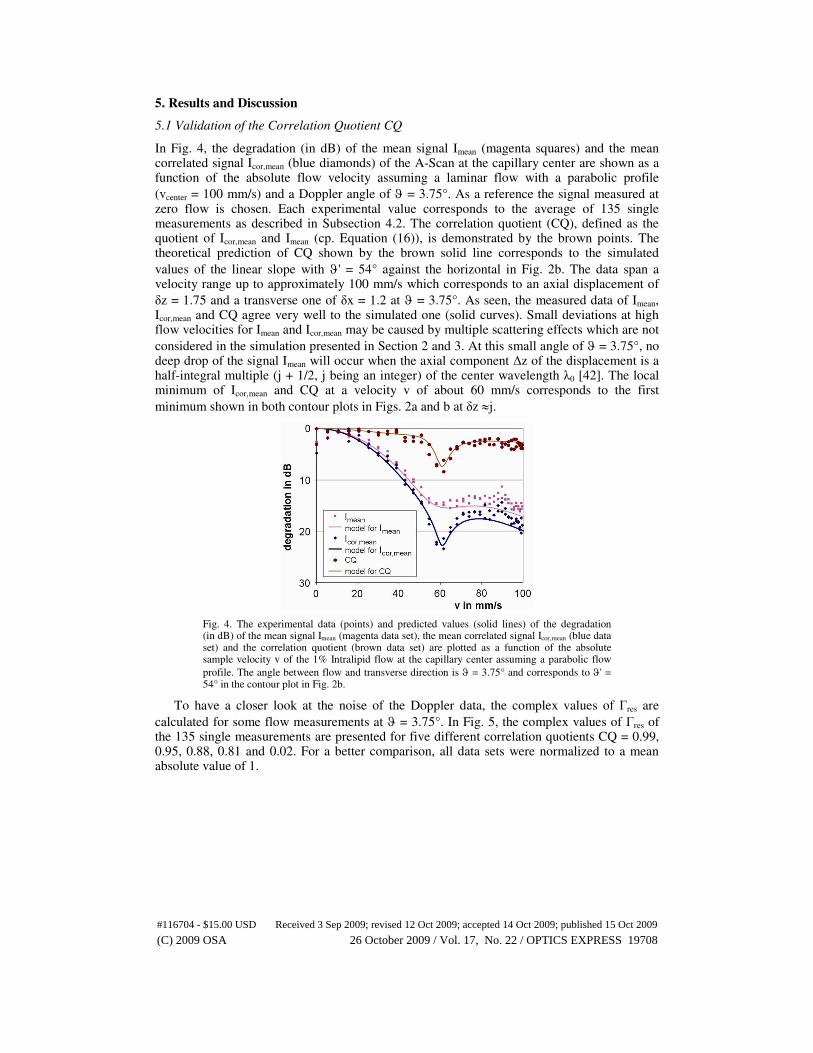
In Fig. 4, the degradation (in dB) of the mean signal Imean (magenta squares) and the mean correlated signal Icor,mean (blue diamonds) of the A-Scan at the capillary center are shown as a function of the absolute flow velocity assuming a laminar flow with a parabolic profile

(vcenter = 100 mm/s) and a Doppler angle of ϑ = 3.75°. As a reference the signal measured at zero flow is chosen. Each experimental value corresponds to the average of 135 single measurements as described in Subsection 4.2. The correlation quotient (CQ), defined as the quotient of Icor,mean and Imean (cp. Equation (16)), is demonstrated by the brown points. The theoretical prediction of CQ shown by the brown solid line corresponds to the simulated

values of the linear slope with ϑ' = 54° against the horizontal in Fig. 2b. The data span a velocity range up to approximately 100 mm/s which corresponds to an axial displacement of

δz = 1.75 and a transverse one of δx = 1.2 at ϑ = 3.75°. As seen, the measured data of Imean, Icor,mean and CQ agree very well to the simulated one (solid curves). Small deviations at high flow velocities for Imean and Icor,mean may be caused by multiple scattering effects which are not

considered in the simulation presented in Section 2 and 3. At this small angle of ϑ = 3.75°, no deep drop of the signal Imean will occur when the axial component ∆z of the displacement is a half-integral multiple (j + 1/2, j being an integer) of the center wavelength λ0 [42]. The local minimum of Icor,mean and CQ at a velocity v of about 60 mm/s corresponds to the first

minimum shown in both contour plots in Figs. 2a and b at δz ≈j.

Fig. 4. The experimental data (points) and predicted values (solid lines) of the degradation (in dB) of the mean signal Imean (magenta data set), the mean correlated signal Icor,mean (blue data set) and the correlation quotient (brown data set) are plotted as a function of the absolute sample velocity v of the 1% Intralipid flow at the capillary center assuming a parabolic flow

profile. The angle between flow and transverse direction is ϑ = 3.75° and corresponds to ϑ' = 54° in the contour plot in Fig. 2b.

To have a closer look at the noise of the Doppler data, the complex values of Γres are

calculated for some flow measurements at ϑ = 3.75°. In Fig. 5, the complex values of Γres of the 135 single measurements are presented for five different correlation quotients CQ = 0.99, 0.95, 0.88, 0.81 and 0.02. For a better comparison, all data sets were normalized to a mean absolute value of 1.



Fig. 5. Scattergram of the complex values of Γres (each with 135 values) for five different velocities. The points were selected by the average phase shift of approximately π/20 (a), π/4 (b), π/2 (c), π (d) and the last point was chosen for the smallest correlation (e). All samples were normalized to a mean of the absolute values of 1. The correlation quotients for these measurements are 0.99 (a), 0.95 (b), 0.88 (c), 0.81 (d) and 0.02 (e). While the individual phase shifts are similar in the first case (a), the scattering increases with smaller correlation. Small values of Γres exhibit a much larger scattering in the phase shift than large values.

The data in Fig. 5a derive from relatively small velocities with a correlation quotient of 0.99 and a phase shift ∆φ of π/20. Due to the Rayleigh distribution of the OCT signal [47], |Γres| obeys an exponential distribution at least for small velocities. Therefore, the 135 individual signals span a large range. As the individual signals are not on a line through the origin, the phase differences calculated from adjacent A-Scans are not constant. Note that ∆φ calculated from small values will have a larger spread than the one from large values (cp. Figure 5a) which again emphasizes the kind of averaging used (Section 4.1). The next points were selected with phase shifts of π/4, π/2 and π. Due to the higher velocity, CQ becomes smaller and results in 0.95, 0.88 and 0.81, respectively. The last point was chosen with nearly zero correlation (CQ = 0.02). In this case, the noise is too high to calculate a mean phase shift from the 135 data points. Note that the correlation between the phases of subsequent A-Scans

does not only disappear for high transverse velocity components (ϑ' < 45°) but also in the

areas around δx ≈0.64 and δz ≈j (j being an integer).

5.2 Mean Error of the Averaged Phase Shift

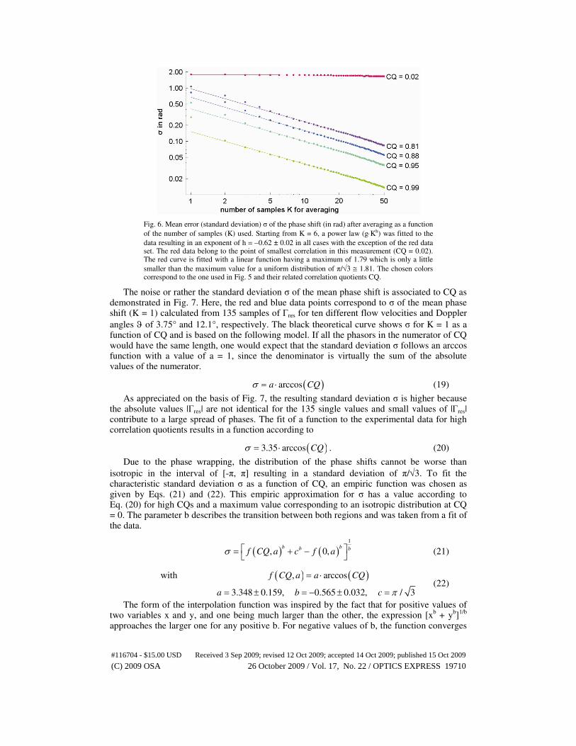
To investigate the performance of the averaging procedure at first, the standard deviation σ of the averaged phase shift according to Eq. (18) is calculated as a function of the number of samples K used for averaging. For this, a specific number of points in the range of K = [1, 50] is 1000 times randomly chosen from the original 135 values shown in Fig. 5. The mean phase shift of the 135 single measurements is subtracted from the calculated mean phase shift of the chosen K values. Subsequently, the standard deviation σ of 1000 of these phase shift differences is determined and plotted in Fig. 6 as a function of K for the five experimental data sets (cp. Figure 5). For the correlation quotients CQ of 0.99 to 0.81, σ decreases rapidly. For values of K larger than five, the drop of σ can be described by a function according to K

h

with h being −0.62 ± 0.02 in all cases apart from the data set with CQ = 0.02. For a Gaussian

distribution of the measurement values, an exponent h of −0.5 would be expected. Probably, the better average of the phase shift is attributed to the exponential distribution. In the case of small numbers of K, an even better reduction of the noise can be noted. For smaller correlation coefficients CQ, a minor decrease of σ can be noted initially which changes to a little stronger drop for a higher number of samples K. For the measurement with almost no correlation (CQ = 0.02), a very small decrease of σ can be denoted despite of the averaging of K = 50 single values.



Fig. 6. Mean error (standard deviation) σ of the phase shift (in rad) after averaging as a function

of the number of samples (K) used. Starting from K = 6, a power law (g⋅Kh) was fitted to the

data resulting in an exponent of h = −0.62 ± 0.02 in all cases with the exception of the red data set. The red data belong to the point of smallest correlation in this measurement (CQ = 0.02). The red curve is fitted with a linear function having a maximum of 1.79 which is only a little

smaller than the maximum value for a uniform distribution of π/√3 ≅ 1.81. The chosen colors correspond to the one used in Fig. 5 and their related correlation quotients CQ.

The noise or rather the standard deviation σ of the mean phase shift is associated to CQ as demonstrated in Fig. 7. Here, the red and blue data points correspond to σ of the mean phase shift (K = 1) calculated from 135 samples of Γres for ten different flow velocities and Doppler

angles ϑ of 3.75° and 12.1°, respectively. The black theoretical curve shows σ for K = 1 as a function of CQ and is based on the following model. If all the phasors in the numerator of CQ would have the same length, one would expect that the standard deviation σ follows an arccos function with a value of a = 1, since the denominator is virtually the sum of the absolute values of the numerator.

( )arccosa CQσ = ⋅ (19)

As appreciated on the basis of Fig. 7, the resulting standard deviation σ is higher because the absolute values |Γres| are not identical for the 135 single values and small values of |Γres| contribute to a large spread of phases. The fit of a function to the experimental data for high correlation quotients results in a function according to

( )3.35 arccos .CQσ = ⋅ (20)

Due to the phase wrapping, the distribution of the phase shifts cannot be worse than

isotropic in the interval of [-π, π] resulting in a standard deviation of π/√3. To fit the characteristic standard deviation σ as a function of CQ, an empiric function was chosen as given by Eqs. (21) and (22). This empiric approximation for σ has a value according to Eq. (20) for high CQs and a maximum value corresponding to an isotropic distribution at CQ = 0. The parameter b describes the transition between both regions and was taken from a fit of the data.

( ) ( )1

, 0,b bb bf CQ a c f aσ = + − (21)

( ) ( )with , arccos

3.348 0.159, 0.565 0.032, / 3

f CQ a a CQ

a b c π

= ⋅

= ± = − ± = (22)

The form of the interpolation function was inspired by the fact that for positive values of two variables x and y, and one being much larger than the other, the expression [x

b + y

b]

1/b

approaches the larger one for any positive b. For negative values of b, the function converges



to the smaller one. In order to have the specific value for CQ = 0, the third term was added in the brackets. In Eq. (22), the fitting parameters a and b are presented as mean values with their standard deviation. Note that the reason for the large standard error is the high correlation of the parameters a and b. Increasing one can be compensated to a high extend by decreasing the other.

Also shown in Fig. 7 is the reduction of the standard deviation σ of the phase shift

determined for selective points and particular values of the measurements with ϑ = 3.75° and K being 5, 10 and 50 (orange, green and magenta points) and is interpolated by a 2nd order polynomial.

Fig. 7. Blue and red data points: Standard deviation σ of the phase shift calculated from 135 samples of Γres for ten different flow velocities (total 1350 values) and different angles (blue

ϑ = 3.75°, red ϑ = 12.1°) as a function of the correlation quotient CQ (Eq. (16)). An empirical

function (black line) was fitted to the data (K = 1) having the correct maximum of π/√3 for a correlation of CQ = 0 and a behavior proportional to arccos near a correlation of CQ = 1. For some data points, the mean error of the phase shift after averaging of K = 5 (orange), 10 (green) and 50 (magenta) samples is added to the plot. This data is interpolated by a 2nd order

polynomial. The scale at the top gives CQ in dB calculated by (−10 log(Icor,mean/Imean)).

The diagram in Fig. 7 includes a second x-axis at the top showing the correlation quotient

CQ in dB (−10·log(CQ)) besides the non-logarithmized values of CQ at the bottom. For a decrease of CQ of only 1 dB, the corresponding σ of the phase shift of the single measurement points (K = 1, black curve) exceeds one. The averaging of K = 5 complex data according to Eq. (17) reduces the value of σ by a factor of three (orange data set). For K = 50 samples, the reduction of σ is about one order of magnitude (magenta data set) in comparison to the case of K = 1. If the decrease of CQ exceeds 5 dB, the noise of the phase shift will increase strongly even for K = 50. On closer examination of the contour plot in Fig. 2b, it can be seen that

CQ = 1 dB corresponds to a maximum transverse displacement δx of 0.4. In contrast, CQ ≥ 5

dB is only achieved for angles ϑ’ smaller than 45° and in the areas with δx ≈0.64 and δz ≈j (j being an integer) which were mentioned in the Sections 2 and 3. Please note that the mean signal Imean also decreases with rising sample velocity and with this other noise factors increase additionally until the phase measurement is not realizable any longer. Even at zero flow conditions, the experimentally measured CQ will always be smaller than one because of Brownian motion in the Intralipid, residual scanner movement and other sources of noise.

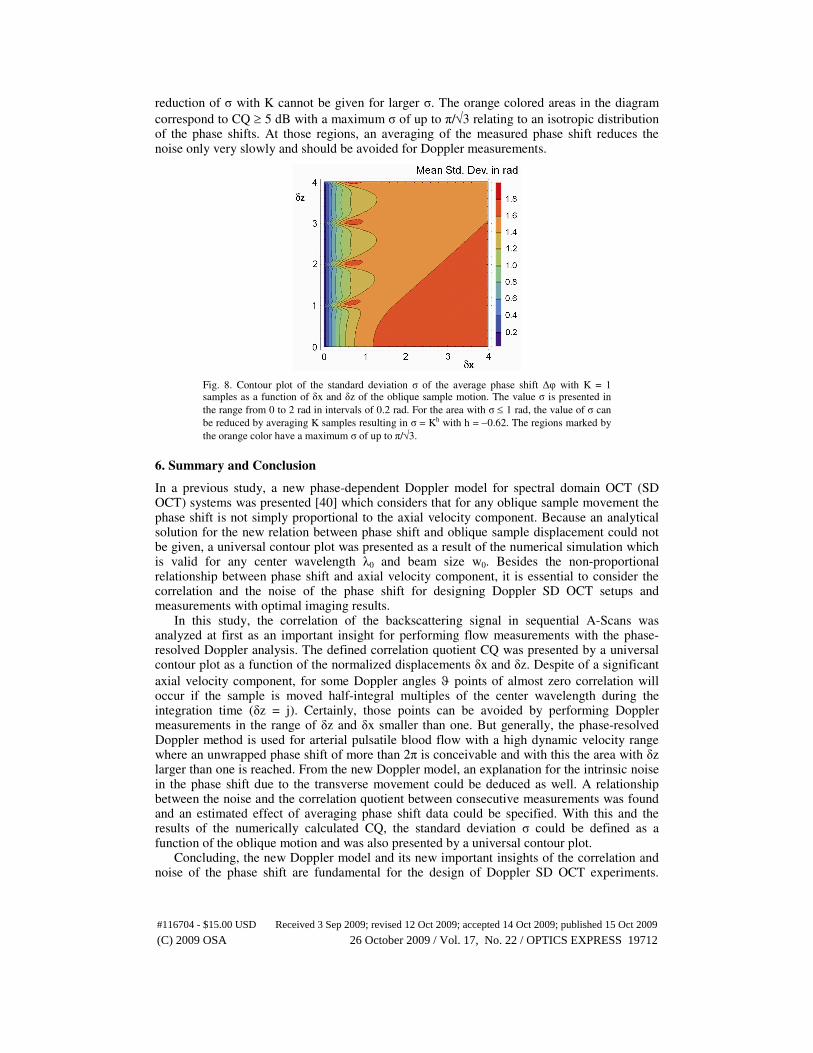
By considering the results of the numerical simulation of CQ (Fig. 2b) and the relation between σ and CQ described by Eqs. (21) and (22), one can calculate σ of the mean phase shift with K = 1 as a function of the oblique sample motion. The resulting contour plot in Fig. 8 shows σ ranging from 0 to 2 rad in intervals of 0.2 rad for δx = δz = [0, 4]. For the areas with σ of approximately smaller than 1 rad, the averaging of K samples of the phase shift

leads to a mean standard deviation σ which decreases in accordance to σ = Kh with h = −0.62

as determined experimentally (cp. Figure 6). Unfortunately, such a general statement of the



reduction of σ with K cannot be given for larger σ. The orange colored areas in the diagram

correspond to CQ ≥ 5 dB with a maximum σ of up to π/√3 relating to an isotropic distribution of the phase shifts. At those regions, an averaging of the measured phase shift reduces the noise only very slowly and should be avoided for Doppler measurements.

Fig. 8. Contour plot of the standard deviation σ of the average phase shift ∆φ with K = 1 samples as a function of δx and δz of the oblique sample motion. The value σ is presented in

the range from 0 to 2 rad in intervals of 0.2 rad. For the area with σ ≤ 1 rad, the value of σ can

be reduced by averaging K samples resulting in σ = Kh with h = −0.62. The regions marked by

the orange color have a maximum σ of up to π/√3.

6. Summary and Conclusion

In a previous study, a new phase-dependent Doppler model for spectral domain OCT (SD OCT) systems was presented [40] which considers that for any oblique sample movement the phase shift is not simply proportional to the axial velocity component. Because an analytical solution for the new relation between phase shift and oblique sample displacement could not be given, a universal contour plot was presented as a result of the numerical simulation which is valid for any center wavelength λ0 and beam size w0. Besides the non-proportional relationship between phase shift and axial velocity component, it is essential to consider the correlation and the noise of the phase shift for designing Doppler SD OCT setups and measurements with optimal imaging results.

In this study, the correlation of the backscattering signal in sequential A-Scans was analyzed at first as an important insight for performing flow measurements with the phase-resolved Doppler analysis. The defined correlation quotient CQ was presented by a universal contour plot as a function of the normalized displacements δx and δz. Despite of a significant

axial velocity component, for some Doppler angles ϑ points of almost zero correlation will occur if the sample is moved half-integral multiples of the center wavelength during the integration time (δz = j). Certainly, those points can be avoided by performing Doppler measurements in the range of δz and δx smaller than one. But generally, the phase-resolved Doppler method is used for arterial pulsatile blood flow with a high dynamic velocity range where an unwrapped phase shift of more than 2π is conceivable and with this the area with δz larger than one is reached. From the new Doppler model, an explanation for the intrinsic noise in the phase shift due to the transverse movement could be deduced as well. A relationship between the noise and the correlation quotient between consecutive measurements was found and an estimated effect of averaging phase shift data could be specified. With this and the results of the numerically calculated CQ, the standard deviation σ could be defined as a function of the oblique motion and was also presented by a universal contour plot.

Concluding, the new Doppler model and its new important insights of the correlation and noise of the phase shift are fundamental for the design of Doppler SD OCT experiments.



Additionally, the new model is essential for the interpretation of measured phase shifts and with this of physiological blood flow velocity profiles.

For a prospective study, the fact of a partial duty cycle is worth to be considered. The advantage of a reduced integration time at a constant A-Scan rate is the reduction of the fringe washout caused by axial and transverse motion leading to higher signals in the case of a fast flow. The SNR decrease induced by the motion of an only lateral scanning sample beam was verified by J. W. You et al. [48] for pulsed illumination with different duty cycles with the result that the SNR is increased for reduced exposure times. However, the signal caused by particles being present in consecutive A-Scans and with this the phase correlation between adjacent A-Scans will be reduced. Therefore, the question if a partial duty cycle at constant A-Scan rate will be beneficial for measuring flow velocities has to be addressed in the future.

Acknowledgements

This research was supported by SAB (Saechsische Aufbaubank, project: 11261/ 1759), the BMBF (Bundesministerium für Bildung und Forschung: NBL 3) and the MeDDrive program of the Medical Faculty Carl Gustav Carus of the University of Technology Dresden.



Date post:	01-Oct-2016
Category:	Documents
Upload:	edmund
View:	212 times
Download:	0 times

Transverse motion as a source of noise and reduced correlation of the Doppler phase shift in...

Documents