Travel Time Models and Throughput Analysis of Dual Load ...

BanD 92

Wissenschaftliche Berichte des Instituts für Fördertechnik und Logistiksysteme des Karlsruher Instituts für Technologie (KIT)

KaTHarIna Dörr

Travel Time Models and Throughput analysis of Dual Load Handling automated Storage and retrieval Systems in Double Deep Storage

Trav

el T

ime

Anal

ysis

of D

ual L

oad

Hand

ling

AS/R

S in

Dou

ble

Deep

Sto

rage

K. D

öRR

Katharina Dörr

Travel Time Models and Throughput Analysis of Dual Load Handling Automated Storage and Retrieval Systems in Double Deep Storage

WiSSenScHAfTLicHe BeRicHTe

institut für fördertechnik und Logistiksystemeam Karlsruher institut für Technologie (KiT)

BAnD 92

Travel Time Models and Throughput Analysis of Dual Load Handling Automated Storage and Retrieval Systems in Double Deep Storage

byKatharina Dörr

Print on Demand 2018 – Gedruckt auf FSC-zertifiziertem Papier

ISSN 0171-2772ISBN 978-3-7315-0793-2 DOI 10.5445/KSP/1000082200

This document – excluding the cover, pictures and graphs – is licensed under a Creative Commons Attribution-Share Alike 4.0 International License (CC BY-SA 4.0): https://creativecommons.org/licenses/by-sa/4.0/deed.en

The cover page is licensed under a Creative CommonsAttribution-No Derivatives 4.0 International License (CC BY-ND 4.0):https://creativecommons.org/licenses/by-nd/4.0/deed.en

Impressum

Karlsruher Institut für Technologie (KIT) KIT Scientific Publishing Straße am Forum 2 D-76131 Karlsruhe

KIT Scientific Publishing is a registered trademark of Karlsruhe Institute of Technology. Reprint using the book cover is not allowed.

www.ksp.kit.edu

Dissertation, Karlsruher Institut für Technologie KIT-Fakultät für Maschinenbau

Tag der mündlichen Prüfung: 12. März 2018Referenten: Prof. Dr.-Ing. Kai Furmans, Prof. Dr.-Ing. Johannes Fottner

Travel Time Models and Throughput

Analysis of Dual Load Handling

Automated Storage and Retrieval Systems

in Double Deep Storage

Zur Erlangung des akademischen Grades eines

Doktors der Ingenieurwissenschaften (Dr.-Ing.)

bei der KIT-Fakultät für Maschinenbau des

Karlsruher Institut für Technologie (KIT)

genehmigte

Dissertation

von

M.Sc. Wi.-Ing. Katharina Alissa Dörr

aus Püttlingen

Tag der mündlichen Prüfung: 12.03.2018

Hauptreferent: Prof. Dr.-Ing. Kai Furmans

Korreferent: Prof. Dr.-Ing. Johannes Fottner

Danksagung

Die vorliegende Arbeit entstand während meiner Tätigkeit als wissen-schaftliche Mitarbeiterin am Institut für Fördertechnik und Logistiksys-teme des Karlsruher Institut für Technologie.

Ich bedanke mich bei meinem Doktorvater Prof. Dr.-Ing. Kai Furmansfür die Betreuung meiner Dissertation. Er hat mir viele Freiheiten gewährtund mir stets großes Vertrauen geschenkt. Prof. Dr.-Ing. Johannes Fottnerdanke ich für die Übernahme des Koreferats. Bei Herrn Prof. Dr. rer. nat.Frank Gauterin bedanke ich mich für die Übernahme des Pürfungsvorsitzesmeiner Promotionsprüfung.

Allen aktiven und ehemaligen Kollegen des IFL danke ich für die an-genehme und inspirierende Arbeitsatmosphäre, die das Erstellen einersolchen Arbeit erleichtert hat. Insbesondere danke ich Marion, Zäzilia undAndreas, die mich immer wieder aufgebaut und unterstützt haben, sowieMelanie und Holger für die kritische Korrektur meiner Arbeit. Außerdemdanke ich allen Abschlussarbeitern und Hiwis, die mit viel Engagement dasThema im Kleinen vorangetrieben haben. Ein großer Dank gilt all meinenwunderbaren Freunden, die immer an mich geglaubt haben. Ihr seid dieBesten.

Meiner Schwester Laura danke ich von ganzem Herzen für stetiges Ermuti-gen und Zureden sowie für die zahlreichen Korrekturrunden. Ganz beson-derer Dank gilt meinen Eltern, da sie mir meine Ausbildung ermöglichthaben. Mama, Papa, Laura - ihr habt mich immer unterstützt und begleitetund zu dem Menschen gemacht, der ich bin. Dafür bin ich sehr dankbar.

Mein allergrößter Dank gilt Christian für unermüdliches Aufbauen, Ertra-gen, Zuhören, Kraftgeben und insbesondere dafür, niemals Zweifel an mirzuzulassen. Danke, dass Du da bist.

Karlsruhe, März 2018 Katharina Dörr

i

Kurzfassung

Vollautomatische Regalanlagen sind essentielle technische Bestandteile

in Lager und Distributionszentren. Da diese Anlagen langfristige Inves-

titionen darstellen, die bei Fehlplanung zu hohen Folgekosten führen

können, sind deren Anwender bei der Auswahl und Dimensionierung auf

verlässliche Ergebnisse aus der Forschung angewiesen. Solche Systeme

werden kontinuierlich von deren Herstellern der Industrie weiterentwick-

elt, was dazu führt, dass die Praxis der wissenschaftlichen Betrachtung oft-

mals voraus ist.

Beispiel eines vollautomatischen Lagers mit doppeltiefen Lagerplätzen und doppelter Las-taufnahme

Eine Möglichkeit die Effizienz vollautomatischer Regalanlagen zu erhöhen,

ist es, die Regale mit doppeltiefen Lagerplätzen auszustatten und ein Re-

galbediengerät mit zweifachem Lastaufnahmemittel zu verwenden, wie in

der Abbildung dargestellt. Diese Variante ermöglicht sowohl eine verbes-

serte Flächennutzung, als auch einen höheren Durchsatz.

iii

Kurzfassung

Obwohl dieser Aufbau häufig in der Praxis anzutreffen ist, fehlt es bisher

an genauen analytischen Formulierungen, sowie einer Betrachtung an-

spruchsvoller Betriebsstrategien, die den Durchsatz steigern können. Das

Ziel dieser Arbeit ist es, diese Forschungslücke in zwei Schrtitten zu

schließen:

Zuerst wird ein grundlegendes analytisches Spielzeitmodell für ein Vier-

fachspiel bei doppeltiefer Lagerung und dem Einsatz eines doppelten

Lastaufnahmemittels formuliert, wobei die Wahrscheinlichkeit für eine

der beiden Reihenfolgen von Einlagerungen und Auslagerungen einen

Paramter des Modells darstellt. Das Modell wird schließlich mit Hilfe einer

Simulation validiert.

Im zweiten Schritt werden Betriebsstrategien, die den Durchsatz im Ver-

gleich zur zufälligen Abarbeitung erhöhen sollen, zusammengestellt. Für

ausgewählte Strategien werden zudem analytische Ausdrücke hergeleitet.

Mit Hilfe der mathematischen Formeln wird der Einfluss verschiedener

Parameter auf die Spielzeit der Strategien untersucht. Um die Strategien

im Rahmen von realistischeren Szenarien zu bewerten, wird ein Simula-

tionsmodell verwendet, wodurch ein Vergleich dieser unter verschiedenen

Einsatzbedingungen ermöglicht wird. Zum Schluss werden die Ergebnisse

der Strategiebewertung diskutiert und Implikationen für deren Anwendung

hinsichtlich unterschiedlicher Rahmenbedingungen abgeleitet.

iv

Abstract

Automated storage and retrieval systems (AS/RSs) are an essential piece of

warehouse technology. As they represent long-term investments, misplan-

ning of these systems results in follow-up costs, which is why practition-

ers are in urgent need of sound research results for selection and sizing of

these systems. The efficiency of AS/RSs is continuously improved by practi-

tioners in industry with the consequence of industrial progress overtaking

theoretical research.

Example of an AS/RS with double deep storage and dual load handling

One possibility to increase the efficiency of automated storage and retrieval

systems is to install a double deep rack structure and the usage of a storage

and retrieval machine with two load handling devices as shown in the il-

lustration. This set-up provides enhanced space utilization and increased

throughput potential.

Although such systems are installed in practice, we encounter the absence

of feasible analytical formulations as well as an investigation of sophisti-

v

Abstract

cated operating strategies to improve throughput. The objective of this

thesis is to close this gap in two steps:

We formulate a general analytical travel time model for the quadruple com-

mand cycle in double deep storage systems with a dual capacity load han-

dling device. Using a parameter that describes the execution order of a

quadruple command cycle, all possible execution orders are included. The

validity of the approach is shown by means of a simulation model.

We compose various routing and sequencing strategies that aim on improv-

ing throughput compared to the random execution. For selected strategies,

analytical formulations are derived. In doing so, we provide basic compo-

nents to describe many additional strategies in a mathematical way. To as-

sess the strategies in consideration of real-world cases, a simulation model

is used to compare strategies for various configurations and settings. Fi-

nally, we discuss results of our simulation studies as well as implications

concerning implementation and application of the strategies in different

environments.

vi

Contents

1 Introduction . . . . . . . . . . . . . . . . . . . . . . . . . . . . . . . 11.1 Problem Description . . . . . . . . . . . . . . . . . . . . . . . . . . 31.2 Scope of this Thesis . . . . . . . . . . . . . . . . . . . . . . . . . . 4

2 Basics of Automated Storage and RetrievalSystems (AS/RSs) . . . . . . . . . . . . . . . . . . . . . . . . . . . 72.1 Categorization and Functionality of AS/RS . . . . . . . . . . . . . 9

2.1.1 Type of the rack . . . . . . . . . . . . . . . . . . . . . . . . . 112.1.2 S/R machine . . . . . . . . . . . . . . . . . . . . . . . . . . . 142.1.3 Handling . . . . . . . . . . . . . . . . . . . . . . . . . . . . . 16

2.2 Operating Policies of AS/RS . . . . . . . . . . . . . . . . . . . . . . 172.2.1 Storage Assignment . . . . . . . . . . . . . . . . . . . . . . . 182.2.2 Routing and Sequencing . . . . . . . . . . . . . . . . . . . . 20

3 Performance of Automated Storage and Retrieval Systems 273.1 Basics of Travel Time Determination . . . . . . . . . . . . . . . . 28

3.1.1 Mathematical Basics . . . . . . . . . . . . . . . . . . . . . . 293.1.2 Modeling of the Storage Rack and the

Movement of the S/R machine . . . . . . . . . . . . . . . . 343.2 Travel Time Determination for AS/RSs . . . . . . . . . . . . . . . 41

3.2.1 Fundamental travel time models . . . . . . . . . . . . . . . 423.2.2 Further Development of the Fundamental

Travel Time Model . . . . . . . . . . . . . . . . . . . . . . . 503.3 Related Work . . . . . . . . . . . . . . . . . . . . . . . . . . . . . . 52

3.3.1 Routing and Sequencing approaches . . . . . . . . . . . . 523.3.2 Travel time models for double deep AS/RS . . . . . . . . . 56

vii

3.3.3 Dual Load Handling combined withDouble Deep Storage . . . . . . . . . . . . . . . . . . . . . . 57

3.3.4 Conclusion on Literature for Travel TimeDetermination and Derivation of the Research Questions 59

Contents

4 Analytical Models for Dual Load Handling,Double Deep AS/RSs . . . . . . . . . . . . . . . . . . . . . . . . . 634.1 Basics for Modeling a Quadruple Command Cycle . . . . . . . . 64

4.1.1 Assumptions . . . . . . . . . . . . . . . . . . . . . . . . . . . 644.1.2 Role of the Execution Order . . . . . . . . . . . . . . . . . . 68

4.2 Approach for the General Model of a RandomQuadruple Command Cycle . . . . . . . . . . . . . . . . . . . . . 714.2.1 Rearrangement - Probability . . . . . . . . . . . . . . . . . 724.2.2 Rearrangement- and Load Handling- Cycle Times . . . . . 844.2.3 Composing the Travel Time Formula . . . . . . . . . . . . . 88

4.3 Calculation Examples for Quadruple Command Cycles . . . . . 904.3.1 Basic Model . . . . . . . . . . . . . . . . . . . . . . . . . . . 914.3.2 SSRR Model . . . . . . . . . . . . . . . . . . . . . . . . . . . 924.3.3 SRSR Model . . . . . . . . . . . . . . . . . . . . . . . . . . . 94

4.4 Model of a Quadruple Command Cycle with Modified Tango . . 964.5 Validation of the Analytical Model . . . . . . . . . . . . . . . . . . 101

4.5.1 Validation Approach . . . . . . . . . . . . . . . . . . . . . . 1014.5.2 Validation Result . . . . . . . . . . . . . . . . . . . . . . . . 1064.5.3 Results when comparing to a realistic set-up . . . . . . . . 1074.5.4 Mean rearrangement distance . . . . . . . . . . . . . . . . 111

4.6 Comparisons and Discussions . . . . . . . . . . . . . . . . . . . . 1144.6.1 Comparison of the derived models . . . . . . . . . . . . . . 1144.6.2 Comparison to previous work . . . . . . . . . . . . . . . . . 121

5 Strategies for Improved Throughput . . . . . . . . . . . . . . . 1255.1 Methodology of Strategy-Definition . . . . . . . . . . . . . . . . . 1255.2 Presentation and Explanation of all Identified Strategies . . . . 130

5.2.1 The Longlist . . . . . . . . . . . . . . . . . . . . . . . . . . . 1315.2.2 Explanation of the Strategy Components . . . . . . . . . . 137

5.3 Analytical Formulation for the Basic Strategies . . . . . . . . . . 1415.3.1 Nearest Neighbor . . . . . . . . . . . . . . . . . . . . . . . . 1435.3.2 Flip Flop (FF1) . . . . . . . . . . . . . . . . . . . . . . . . . . 1535.3.3 Shortest Leg (SL1) . . . . . . . . . . . . . . . . . . . . . . . . 1565.3.4 Multiple Storage (MS1) . . . . . . . . . . . . . . . . . . . . . 160

viii

5.3.5 Validation . . . . . . . . . . . . . . . . . . . . . . . . . . . . 1675.4 Calculated Comparison . . . . . . . . . . . . . . . . . . . . . . . . 168

5.4.1 Static results . . . . . . . . . . . . . . . . . . . . . . . . . . . 1695.4.2 Comparison of all models for varied parameters . . . . . . 170

Contents

5.4.3 Computation of selected intersections . . . . . . . . . . . . 1745.4.4 Summary . . . . . . . . . . . . . . . . . . . . . . . . . . . . . 177

6 Performance Analysis using Simulation . . . . . . . . . . . . . . 1796.1 Implementation of the strategies in the simulation model . . . . 180

6.1.1 Selection of Strategies: The Short List . . . . . . . . . . . . 1806.1.2 Adjustments for Implementation of Strategies . . . . . . . 183

6.2 Set - Up of the Simulation Studies . . . . . . . . . . . . . . . . . . 1846.2.1 Description of Control Parameters . . . . . . . . . . . . . . 1856.2.2 Parameter Settings . . . . . . . . . . . . . . . . . . . . . . . 1896.2.3 Performance Indicators . . . . . . . . . . . . . . . . . . . . 1916.2.4 Statistical Validation of Simulation Results . . . . . . . . . 191

6.3 Results: Behavior of Strategies . . . . . . . . . . . . . . . . . . . . 1956.3.1 High Level Results . . . . . . . . . . . . . . . . . . . . . . . . 1956.3.2 Influence of the options for selection

of retrieval requests . . . . . . . . . . . . . . . . . . . . . . . 2026.3.3 Influence of the filling level . . . . . . . . . . . . . . . . . . 2066.3.4 Influence of the SKUs’ Gini coefficicent . . . . . . . . . . . 2106.3.5 Selected Cases . . . . . . . . . . . . . . . . . . . . . . . . . . 213

6.4 Conclusion: Performance of Operating Strategies for QC . . . . 2156.4.1 Implications of the Simulation Results . . . . . . . . . . . . 2156.4.2 Comparison between Analytical and Simulation Results . 217

7 Conclusion . . . . . . . . . . . . . . . . . . . . . . . . . . . . . . . . 2197.1 Summary of the Thesis . . . . . . . . . . . . . . . . . . . . . . . . 2197.2 Conclusion and Outlook . . . . . . . . . . . . . . . . . . . . . . . 222

Nomenclature . . . . . . . . . . . . . . . . . . . . . . . . . . . . . . . . 225

References . . . . . . . . . . . . . . . . . . . . . . . . . . . . . . . . . . 229

List of Figures . . . . . . . . . . . . . . . . . . . . . . . . . . . . . . . . 239

List of Tables . . . . . . . . . . . . . . . . . . . . . . . . . . . . . . . . 247

A Additional Analytics . . . . . . . . . . . . . . . . . . . . . . . . . . 251

ix

B Simulation Studies . . . . . . . . . . . . . . . . . . . . . . . . . . . 267

1 Introduction

Confidence

-M. Kiehn, née Becker

As the global volume of trade and flow of goods is continuously increasing,

cross-docking and warehousing is more important than ever. Within these

logistical hubs, efficient technology is a crucial element to guarantee both

supply chain performance and reliability. Automated storage and retrieval

systems (AS/RSs), representing the combination of storage equipment and

controls to automatically store and retrieve goods, are one of the key ele-

ments used in this context.

However, automated storage and retrieval systems entail significant invest-

ments. Besides, they are quite inflexible in terms of physical changes, once

they are installed (Bartholdi and Hackman 2016, p. 200). Therefore, de-

tailed knowledge about the performance of an AS/RS is needed to capture

full economic benefit. An exact evaluation of its throughput is required

to meet external requirements (i.e. customer demands) on the one hand,

and to ensure a smooth operation among connected processes as found

in distribution centers on the other hand. Reliable planning of automated

storage and retrieval systems prevents follow-up costs, while solid evalua-

tion of changing external conditions ensures timely modifications of these

rather inflexible systems. Both reasons emphasize why practitioners are in

urgent need of sound research results to determine these kind of systems

mathematically. For standard systems that use traditional racks and single-

load storage and retrieval machines, results have been presented since the

1970s. Nowadays, official guidelines from F.E.M exist.

1

1 Introduction

Due to their popularity, the efficiency of automated storage and retrieval

systems is continuously improved by various new applications and adap-

tions that are developed by practitioners in industry. In that way, industrial

progress has overtaken academic research in some points. As a result, for

some new applications, a fundamental mathematical description is not ex-

isting so far.

One possibility to increase the efficiency of automated storage and retrieval

systems is to install a double deep rack structure and to use a storage and

retrieval machine with two load handling devices. This allows enhanced

space utilization and increased throughput potential. Figure 1.1 gives an

example of this specific AS/RS design. Although such systems are applied

in practice, we encounter the absence of feasible analytical formulations.

Therefore, it is highly important to gain knowledge about this kind of AS/RS.

Figure 1.1: Example of an AS/RS with double deep storage and a dual load handling device

The objective of this thesis is to close this gap and to provide profound re-

search in the field of AS/RSs which allow double deep storage and operate

with dual capacity load handling devices. A general valid, analytical travel

time formula for a random quadruple command cycle with double deep

storage systems is developed. We study routing and sequencing policies

(referred to as strategies) to improve throughput compared to a random ex-

ecution of requests and mathematically derive related models for quadru-

ple command cycles that consist of two storage and two retrieval opera-

2

1.1 Problem Description

tions. For selected strategies, we evaluate their potential for reduction of

travel times with extensive simulation studies.

1.1 Problem Description

We differentiate two major research segments of our examination of double

deep, dual load handling AS/RSs, resulting in two leading research ques-

tions.

First segment: Existing models and approaches of travel time determina-

tion for a quadruple command cycle in double deep storage systems have

significant limitations. They do not allow for total randomized storage, all

possible orders of execution and the different rearrangement options. For

the first segment of research we formulate the leading research question.

Question 1: How can the mean travel time of a randomly

executed quadruple command cycle be determined?

Related questions are:

• What are essential assumptions for a randomly performed

quadruple command cycle?

• How can a randomly performed quadruple command cycle be

defined?

Second segment: Promising approaches of routing and sequencing strate-

gies to improve throughput in AS/RSs are already known. While for tradi-

tional single deep AS/RSs analytical models exist, this is not the case for

double deep environments. As available models are formulated with differ-

ent assumptions and conditions, no consistent basis for a comparison of

all possible strategies exists. The second segment of research is defined by

the leading research question.

Question 2: How can sophisticated operating strategies be

described and in which cases do they provide a travel time

advantage?

3

1 Introduction

Related questions are:

• Which circumstances and conditions are relevant for the implemen-

tation of these strategies?

• How do they change in performance under consideration of sequenc-

ing of retrieval requests, demand structure of stock keeping units

(SKU) or technical restrictions?

• How can they be analytically described? Can their travel times be de-

termined mathematically?

1.2 Scope of this Thesis

This thesis is divided into six chapters that are structured in the following

way:

In Chapter 2 we provide basic knowledge on automated storage and re-

trieval systems. First we describe the structure and technical characteris-

tics of AS/RSs. Important fundamentals with regard to organizational and

qualitative descriptions are presented. Subsequently, the operation mode

and common policies for storage, retrieval and sequencing are presented.

Chapter 3 focuses on the quantitative characterization of AS/RS. First, a

formal description of storage systems is presented and mathematical ba-

sics are recapitulated. The derivation of fundamental travel time models,

which are used to evaluate performance of AS/RS, are explained within a

literature review. The second part of this chapter provides a review of ex-

isting research in relation to this thesis. In doing so, the research gap is

emphazised as we present what is missing in existing research.

Building on this, Chapter 4 covers the first research segment. We formulate

a general analytical travel time model for the quadruple command cycle in

double deep storage systems with dual load capacity load handling device.

Using a parameter that describes the execution order of a quadruple com-

mand cycle, all possible executions order are included. The validity of the

approach is shown by means of a simulation model. The chapter closes

with a comparison to existing approaches.

4

1.2 Scope of this Thesis

Chapter 5 and 6 address the second research segment. Strategies are com-

posed from existing approaches found in literature as well as from prac-

tical experience and a classification of strategies in a double deep storage

environment with a dual capacity load handling device is developed. For

selected strategy groups, analytical formulations are derived. In doing so,

we provide basic components to describe many additional strategies in a

mathematical way. To assess the strategies in consideration of real-world

cases, a simulation model is used to compare strategies for various config-

urations and settings. Finally, we discuss results of our simulation studies

as well as implications concerning implementation and application of the

strategies in different environments.

Figure 1.2 shows the methodical categorization of the main parts and their

coherence. While Chapter 4 follows a quantitative approach and Chap-

ter 6 presents an empirical examination, chapter 5 combines both aspects.

Composition and classification of strategies is a qualitative task, modeling

their travel times based on the results of Chapter 4 is a quantitative task.

EmpiricalAnalytical

Chapter 4

Performance evaluation for quadruple command cycles in double deep

Chapter 6Chapter 5

Figure 1.2: Methodical categorization of the main chapters

Finally, the results and accomplishments are summarized in Chapter 7.

5

2 Basics of AutomatedStorage and RetrievalSystems (AS/RSs)

We think too much

and feel too little.-C. Chaplin

Warehouses are an inherent part of all flow of goods. They are required

due to many different reasons such as ensuring supply of material, balanc-

ing different fluctuations of supply and demand, sorting and composing

of orders, processing or venturing (Martin 2014, p. 336). At the same time,

warehouses differ depending on the particular circumstances and require-

ments. We do not consider different motivations and functions of ware-

housing in greater details, while interested readers are recommend to study

Martin (2014), Arnold, Isermann, Kuhn, Tempelmeier and Furmans (2008),

Rushton (2017) and Bartholdi and Hackman (2016).

The focus of this chapter is to provide basic knowledge in the context of

automated storage and retrieval system (AS/RSs). First, we introduce how

different warehouse types can be categorized and how such systems can be

classified. Afterwards, we present the technology of an AS/RS and explain

how such systems are typically operated.

In literature, there are many ways of grouping warehouses, for examples by

• The function or the location of the warehouse within

the supply chain,

7

2 Basics of Automated Storage and Retrieval Systems (AS/RSs)

• The type of the goods stored,

• The type of the unit load, e.g. pallets, bins or boxes,

• The warehouse design,

• The technology applied to handle goods.

The classification of warehouse design or warehouse type is not consis-

tent in literature. A widely used way is to categorize warehouses into three

groups: Floor storage, static rack- and dynamic rack storage (Arnold, Is-

ermann, Kuhn, Tempelmeier and Furmans 2008, p. 648 ff.). Floor storage

can be further divided into block or line storage, done by stacking pallets

accordingly (Arnold and Furmans 2009, p. 191). Static rack storage refers

to all types of systems where the storage unit remains at the same posi-

tion. They are suitable for different types of unit loads. Common examples

are shelving storage systems, adjustable pallet racking and high bay storage

systems (Rushton 2017, p. 24 ff.). In dynamic rack systems, storage units are

moved between put-away and picking, either by movement of the storage

units itself or by movement of the rack. Examples of such types are flow

racks, mobile racking systems or carousel systems. Apart from a complete

manual operation, handling of goods can be realized in different ways us-

ing different technologies such as traditional fork lifts, other types of fork

lift trucks (e.g. reach trucks and narrow-aisle trucks), storage and retrieval

machines and special equipment such as robots and cranes (Arnold and

Furmans 2009, p. 190). Figure 2.1 summarizes how automated AS/RS are

defined in regard to warehouse design and handling technology.

AS/RSs are fully automated, computer controlled systems with fixed-path

stacker cranes, also referred to as storage and retrieval machines (S/R ma-

chines), serving a static storage rack.

Note that another type of AS/RS, which gained a lot of attention in recent

time, are systems using autonomous vehicle storage and retrieval systems

(Roodbergen and Vis 2009). In these systems, horizontal and vertical trans-

port of loads is separated from each other: The rail-guided vehicles move

horizontally along aisles and cross-aisles. Lifting mechanisms, often lo-

cated at the front side of the rack, are utilized for the transport in vertical

8

2.1 Categorization and Functionality of AS/RS

direction. Another common name of these systems is shuttle based stor-

age and retrieval systems (SBS/RS), where the term shuttle is applied to the

vehicles. Epp (2017) provide an extensive literature review and comprehen-

sive throughput evaluations of such systems.

Floor storage

Static rackS

tora

ge

an

d

retr

ieva

l

ma

ch

ine

s

Fo

rk lift

(tru

cks)

Sp

ecia

l fo

rk lift

tru

cks

Cra

ne

s, ro

bo

ts

an

d s

pe

cia

l

eq

uip

me

nt

Dynamic rack

AS/RS

Wa

reh

ou

se

de

sig

n

Handling of goods

Figure 2.1: Characteristics of AS/RSs in terms of warehouse design and handling of goods.

2.1 Categorization andFunctionality of AS/RS

Automated storage and retrieval systems are a preferred and commonly

used warehouse type as they offer many advantages (Arnold, Isermann,

Kuhn, Tempelmeier and Furmans 2008, p. 647) Due to a high degree of

automation, labor costs are reduced whereas picking quality is increased

compared to non-automated systems. Moreover, they provide a high space

utilization which reduces the floor space required. Compared to other sys-

tems, AS/RSs yield high investment costs, e.g. for storage equipment and

control systems, and less flexibility, which is why exact dimensioning is

important. However, design and dimensioning depend on throughput re-

9

quirements and thus exact throughput determination is crucial to make

an adequate design choice.


a) b)

Figure 2.2: a) Top view of a schematic illustration for traditional AS/RS b) Example of anminiload AS/RS (Mecalux 2017a)

AS/RSs typically consist of racks, storage and retrieval machines with load

handling devices, I/O points and a centralized control computer that is

connected to the warehouse management system. S/R machines run up

and down the aisles between the racks to pick-up and deliver loads. The

racks consist of metal structures, forming the storage locations for the

loads. The I/O points are location where loads are picked up before their

storage and dropped of after being retrieved from the rack.

The traditional version of an AS/RS is a fully automated, unit-load, aisle-

captive (one S/R machine per aisle) system with single-deep storage lo-

cations. Figure 2.2 a) shows a schematic illustration of the structure of a

traditional AS/RS in a top view. ‘Miniload’ systems are the small versions

of AS/RSs and basically consist of the same elements. Generally, they are

lighter in structure, and achieve much higher values of velocity and accel-

eration (Arnold, Isermann, Kuhn, Tempelmeier and Furmans 2008, p. 666).

Part b) of Figure 2.2 shows the side-view of a single aisle in a miniload sys-

tem with plastic boxes as handling units. To give an overview of the various

system options for AS/RSs, Roodbergen and Vis (2009) present a compre-

10

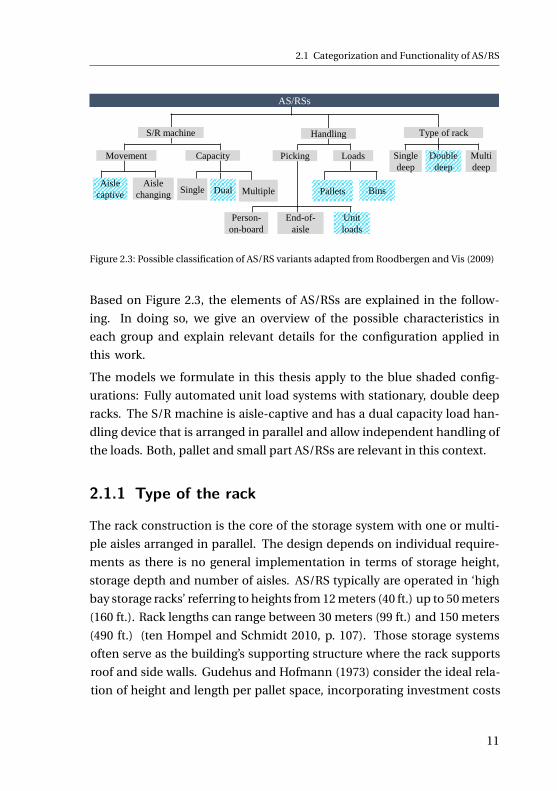
hensive classification of AS/RS. Figure 2.3 shows a modified classification

derived from theirs.


AS/RSs

Single

deep

Double

deep

Pallets BinsAisle

captive

Aisle

changingSingle Dual

Unit

loads

End-of-

aisle

Person-

on-board

HandlingS/R machine Type of rack

CapacityMovement LoadsPicking

Multiple

Multi

deep

Figure 2.3: Possible classification of AS/RS variants adapted from Roodbergen and Vis (2009)

Based on Figure 2.3, the elements of AS/RSs are explained in the follow-

ing. In doing so, we give an overview of the possible characteristics in

each group and explain relevant details for the configuration applied in

this work.

The models we formulate in this thesis apply to the blue shaded config-

urations: Fully automated unit load systems with stationary, double deep

racks. The S/R machine is aisle-captive and has a dual capacity load han-

dling device that is arranged in parallel and allow independent handling of

the loads. Both, pallet and small part AS/RSs are relevant in this context.

2.1.1 Type of the rack

The rack construction is the core of the storage system with one or multi-

ple aisles arranged in parallel. The design depends on individual require-

ments as there is no general implementation in terms of storage height,

storage depth and number of aisles. AS/RS typically are operated in ‘high

bay storage racks’ referring to heights from 12 meters (40 ft.) up to 50 meters

(160 ft.). Rack lengths can range between 30 meters (99 ft.) and 150 meters

11

(490 ft.) (ten Hompel and Schmidt 2010, p. 107). Those storage systems

often serve as the building’s supporting structure where the rack supports

roof and side walls. Gudehus and Hofmann (1973) consider the ideal rela-

tion of height and length per pallet space, incorporating investment costs


for the steel construction. The dimensions of the rack system influence the

total number of storage positions. The determination of the needed num-

ber of storage positions depends on the inventory development over time

for the different types of goods (Arnold and Furmans 2009, p. 176 f.).

However, design of the storage rack takes into account several more aspects,

such as the direction of storage, i.e. is longitudinal or lateral to the rack, or

the number of shelf uprights and the possible number of storage locations

between them. The positioning of input and output locations that can be

separated from each other, e.g. at different levels of height, is another de-

sign choice. For further explanation see ten Hompel and Schmidt (2010,

p. 77), Martin (2014, p. 369) and Rushton (2017, p. 262).

For stationary racks operated by S/R machines, a distinction is made be-

tween single-, double-, and k- deep.

Single deep storage racks

Single deep storage systems represent the standard and the most common

case of line storage with racks. All storage units are positioned next to each

other within one plane where every unit is directly accessible from the aisle.

Both, Figure 2.2 a) and Figure 2.2 b) show single deep storage.

Double deep storage racks

In double deep storage systems, two storage positions are located behind

each other. Together, the position at the front, located next to the aisle, and

the position behind form a storage lane. Figure 2.4 shows the top view of an

aisle with double deep storage positions on both sides. Both positions of a

storage lane are accessed from the aisle. The load handling device is able to

reach both positions, through telescopic forks or similar mechanisms.

12


Figure 2.4: Top view of an aisle with double deep storage racks

Due to the reduced number of aisles, double deep storage allows denser

storage and therefore can accommodate between 30% (Arnold, Isermann,

Kuhn, Tempelmeier and Furmans 2008, p. 380) and 40% (Bartholdi and

Hackman 2016, p. 54) more storage positions at the same floor space. How-

ever, direct access to the rear position is not always possible. If both storage

positions of a storage lane are occupied, the rear position can only be ac-

cessed by rearranging the load at the front position. Consequently, the av-

erage access time is decreased because of such rearrangement operations.

Multiple deep storage racks

A k-deep storage system consists of k storage positions in one storage lane,

also referred to as channel. As load handling devices with telescopic tech-

nology are limited in their range, different technologies are needed to serve

all positions. Therefore, load handling for multiple deep storage, is differ-

ent from those for single- or double deep racks in most cases. In the con-

text of AS/RSs, this is typically achieved by shuttle based systems (Rushton

2017, p. 254). Multiple deep storage offers the advantage of high space uti-

lization. However, especially if a channel can not be allocated to a single

SKU type, a high number of rearrangement operations is provoked. Con-

sequently, multiple deep storage is suitable for a small variety of different

goods to efficiently use the capacity of channels.

13


One mast design Two mast design

a) b)

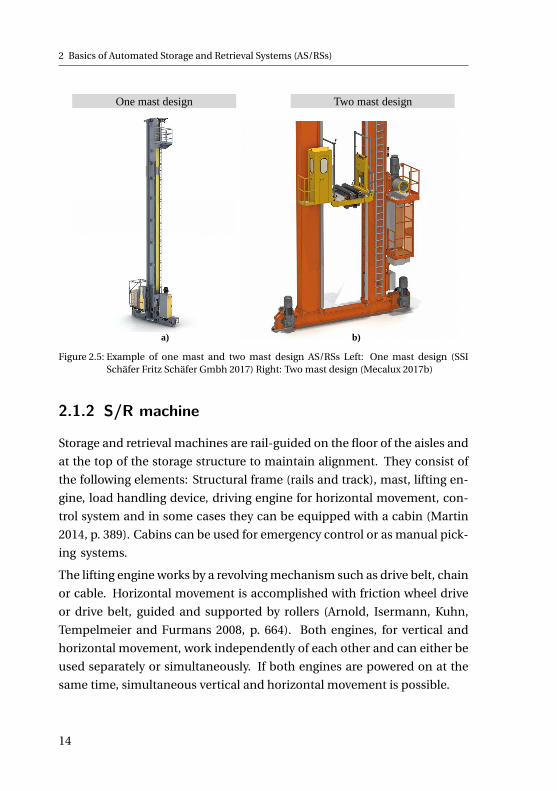
Figure 2.5: Example of one mast and two mast design AS/RSs Left: One mast design (SSISchäfer Fritz Schäfer Gmbh 2017) Right: Two mast design (Mecalux 2017b)

2.1.2 S/R machine

Storage and retrieval machines are rail-guided on the floor of the aisles and

at the top of the storage structure to maintain alignment. They consist of

the following elements: Structural frame (rails and track), mast, lifting en-

gine, load handling device, driving engine for horizontal movement, con-

trol system and in some cases they can be equipped with a cabin (Martin

2014, p. 389). Cabins can be used for emergency control or as manual pick-

ing systems.

The lifting engine works by a revolving mechanism such as drive belt, chain

or cable. Horizontal movement is accomplished with friction wheel drive

or drive belt, guided and supported by rollers (Arnold, Isermann, Kuhn,

Tempelmeier and Furmans 2008, p. 664). Both engines, for vertical and

horizontal movement, work independently of each other and can either be

used separately or simultaneously. If both engines are powered on at the

same time, simultaneous vertical and horizontal movement is possible.

14


The mast is usually made of aluminum or steel, nowadays also construc-

tions made of fiber composites exist (Gebhardt Fördertechnik Gmbh 2017).

A distinction is made between one and two mast systems, with the latter

ones needed to reach heights of 45 meters (147 ft.) and more. The load han-

dling devices of two mast systems are mounted between the mast, which

allows them to bear greater loads, but also makes them heavier and more

expensive. Figure 2.5 gives an example of both an S/R machine with a one-

mast design in part a) and with a two-mast design in part b).

The relation between the number of aisles and the number of S/R machines

is not necessarily one to one. If one S/R machine serves more than one

aisle, it is able to change aisles by curved rails or with transfer cars that are

located at the front side of the racks. We focus our study on aisle-captive

systems that have one S/R machine in each aisle.

Capacity

Development of AS/RSs has constantly been evolved over the past decades.

Nowadays, systems for dual and multiple load handling exist. In most cases,

multiple load handling occurs along with two-mast systems. Figure 2.6

shows two possibilities of a dual load handling device. Figure 2.6 b) de-

picts a dual load handling device with two independent forks for pick-up

and deposition. Figure 2.6 a) illustrates dual load handling with a double

deep load handling device, which requires a double deep aisle (Arnold, Is-

ermann, Kuhn, Tempelmeier and Furmans 2008, p. 666). Here, the units

are positioned behind each other instead of side by side. Another option

for dual load handling are load handling devices where the loads are posi-

tioned above each other. In the remainder of this work, we assume the load

handling devices to be arranged in parallel and independent of each other

as shown in Figure 2.6 b).

Miniload systems often provide multiple load handling devices of four or

six units (Rushton 2017, p. 262).

15


shuttle’). Nonetheless, storage and retrieval systems using shuttle vehicles,

referring to tier captive or aisle captive satellites, are called shuttle based

systems. For clarity, we use the term load handling device (LHD) instead of

shuttle in the context of handling and movement of loads.

a) b)

Figure 2.6: Two possibilities to realize dual load handling. a): With the loads behind one an-other in a double deep aisle (Gebhardt Fördertechnik Gmbh 2017) b): Loads nextto each other in the direction of the aisle(MIAS Group 2017)

2.1.3 Handling

Usually, AS/RSs handle goods in standardized containers. Two main types

of loads can be distinguished: Pallets on the one hand and bins on the other

hand. For the picking of loads, we can distinguish between picking of only

full unit loads and parts of it. If partial unit loads are required, there are

two common possibilities that integrate handling of partial amounts in the

AS/RS.

Cabins that are mounted at the mast of the S/R machine represent one pos-

sibility to allow manual picking. In this set-up, referred to as person-on-

board system, workers travel to the storage positions and pick-up single

items from the loads, while the loads remain in the rack.

For the second option, loads are automatically retrieved and delivered to a

picking workstation. There, workers take out single items before the load is

stored back in the system. The workstations are often located at the front-

side of the rack and referred to as end-of-aisle systems.

16

Note that the load handling device is often referred to as shuttle in litera-

ture, especially if it is capable of loading more than one unit (e.g. ‘dual-

2.2 Operating Policies of AS/RS

In the following, we consider the handling technology of unit loads. By han-

dling technology we refer to the mechanisms used to retrieve the loads from

and deposit the loads into the rack.

Handling of pallets is usually done with telescopic forks that extend under

the pallet, lift them shortly by the lifting engine and then retract. For double

deep storage, handling of pallets requires more space in vertical direction

because of greater bending of the forks.

There are different technologies for the handling of bins. The possibili-

ties are pushing/pulling mechanisms with fingers that move the load or

grabbing the load with telescopic side clamps. Another option are fork-

like telescopes that extract under the units, if possible, or use belt convey-

ors.(Arnold, Isermann, Kuhn, Tempelmeier and Furmans 2008, p. 666 f.)


AS/RSs automatically perform storage and retrieval operations controlled

by a computer system. Basically, loads are picked-up at the I/O point and

moved to their storage location, whereas units to be retrieved are picked-

up at their storage location in the rack and are moved to the I/O position

where they are deposited. There are a number of control policies that can

determine the possible actions performed by an AS/RS (Roodbergen and

Vis 2009). This section explains the basic operating modes of an AS/RS and

gives an overview of different policies. There is no standardized set of poli-

cies in the context of AS/RSs design and operation. In literature, policies

are presented with different categorizations and levels of detail. Some of

the most common control policies are routing policies, sequencing policies

and storage assignment policies. Roodbergen and Vis (2009) also consider

batching and dwell-point policies. Vasili, Tang and Vasili (2012) also incor-

porate load shuffling. Furthermore, Kraul (2010) and Atz (2016) distinguish

between storage policy, retrieval policy, idle time policy and aisle changing

policy. These groups are not mutual exclusive. Roodbergen and Vis (2009)

17


provide an extensive summary of literature and a comprehensive descrip-

tion for AS/RSs’ control policies.

We address the question of how the performance of an AS/RS (operating

under different control policies) is determined based on travel times mod-

els in Chapter 3.

2.2.1 Storage Assignment

A storage assignment policy is a rule that determines how to choose stor-

age positions within the rack. In literature, most attention is paid to ran-

dom storage assignment and class-based storage assignment. Less com-

mon are dedicated storage assignments and full-turnover based storage as-

signments, whereas closest open location storage assignments occurs more

rarely. At dedicated storage assignment, each SKU type is assigned to a fixed

number of storage locations that are exclusively used for this type. There-

fore, for each SKU there must be enough space available for the maximum

number of units that may be stored at the same time. For closest open lo-

cation storage assignment, the nearest empty location with respect to the

I/O point is used. Full turnover based assignment is a special case of class

based storage assignment which is discussed below.

Random Storage Policy

In random storage assignment, every load can be assigned to each avail-

able storage position within the rack. Consequently, each empty position

has the same probability of being chosen as storage position and the units

are evenly allocated throughout the rack. Due to pooling effects, i.e., the

balancing of peak demands for different SKUs, less total storage space is

needed compared to dedicated storage assignment. Moreover, random

storage assignment requires low organizational effort and is a baseline for

strategies that optimize throughput and cycle times.

18


Class Based Storage Policy

With classed based storage policies, all SKUs are analyzed and grouped ac-

cording to their demand frequencies. The available storage space is divided

into a certain number of classes, each belonging to one of the groups. The

objective is to decrease mean travel times by locating those with the high-

est demand frequency closest to the I/O point. Within each class, random

storage assignment is applied.

x

y

I/O

A

B

C

Figure 2.7: Example of class based storage policy with a rack divided into three different zones

The challenges are to determine the number of classes, to identify the num-

ber of products assigned to each class and to determine the location of

each class within the storage rack. A common practice is to divide SKUs

by means of an ABC analysis into three groups and use the result for the

classification of the rack as shown in Figure 2.7 (Roodbergen and Vis 2009,

p. 349). The aim of this approach is to limit the constitution effort for the

class definition. Glass (2009, p. 47) emphasizes that many authors conclude

that with such a small number of classes a majority of the potential for op-

timization is covered. In the extreme case of one class for each individual

SKU, class based storage assignment turns into full turnover based stor-

age assignment. In this case, the advantages of the random storage policy

within the classes disappear, whereas organizational requirements increase

(Kraul 2010, p. 48).

19


2.2.2 Routing and Sequencing

To provide a better understanding of routing and sequencing, we first ex-

plain the fundamental types of operation, before we go into more detail

with routing and sequencing.

Type of operation

The Type of operation defines which command cycle is applied to oper-

ate an AS/RS.

Traditional AS/RSs that have a single capacity load handling device perform

single or dual command cycles. In a single command cycle (SC), either a

single storage or a single retrieval operation is performed. A storage cycle

consists of picking up the load at the I/O point, traveling of the S/R machine

to the storage position, placing the load into the rack and returning back to

the I/O point. A retrieval cycle is performed similarly. Consequently, during

a storage cycle the return travel is an empty run of the S/R machine, while

for a retrieval cycle, the travel to the storage position is an empty run.

In a dual command cycle (DC), storage and retrieval are combined in one

cycle as shown in Figure 2.8.

x

y

I/O

Empty run

LoadedStorage (1)

Retrieval (2)

Figure 2.8: Example of a dual command cycle showing the movement of the S/R machine

In a first step, the load is picked-up at the I/O point, transported to its stor-

age location and stored into the rack (1). Subsequently, the S/R machine

travels to the retrieval location (2), the load is picked-up and returned to

20


the I/O point. The travel distances within the rack, here between (1) and (2),

are also called travel-between distances. Figure 2.8 shows a schematic side

view of a storage rack and gives an example for the movement of the S/R

machine while performing a dual command cycle. This way, empty trav-

els as well as the time needed per operation can be reduced (Bartholdi and

Hackman 2016, p. 202). While both storage and retrieval requests are avail-

able, it is always beneficial to perform dual command cycles to increase

overall throughput. However, in cases when storage or retrieval are critical,

performing only one type of a single command cycle may be appropriate,

because the throughput of the individual type of operation (storage or re-

trieval) decreases with dual command cycles.

In a system with multiple load handling, command cycles of higher order

are possible. With a dual capacity load handling device, two storage oper-

ations and two retrieval operations are possible in a single cycle, which is

called a quadruple command cycle (QC). Similarly, for a load handling ca-

pacity of three units, sextuple command cycles become feasible by storing

and retrieving three units each. Figure 2.9 illustrates a simplified example

for the procedure of a quadruple and a sextuple command cycle. In both

examples of Figure 2.9, all storage operations are performed first. However,

the order can change, because retrieval operations are possible with at least

one empty load handling device.

x

y

I/O

Storage

Retrieval

Storage

Retrieval

x

y

I/O

Storage

Retrieval

Storage

Retrieval

Storage

Retrieval

Figure 2.9: Simplified example of a quadruple and sextuple command cycle

21


Storage and retrieval selection

Different degrees of freedom are possible for the selection of storage and

retrieval locations of an upcoming command cycle. In this thesis we as-

sume the following:

Freedom of storage selection is determined by the storage assignment pol-

icy (see subsection 2.2.1), assuming more than one possible open location.

The storage units remain in their order of arrival . Rearranging the order

requires adequate space and conveyor technology, because they are repre-

sented by physical units (Kraul 2010, p. 43). Moreover, storage requests are

not time-critical in general (Roodbergen and Vis 2009). As a consequence

we do not consider the rearrangement of the order of storage requests.

Retrieval list based on the SKUs that are requested for retrieval

A B C A E G D ….

Select the unit with the earliest storage time (FCFS)

Choose from all units, e.g. a random one

A1 A2 A3 A4 A5 A6 ….

B1 B2 B3 B4 B5 B6 B7Record of all stored units of SKU

type “B” in order of their entry

Record of all stored units of SKU type

“A” in order of their entry

Retrieval Policy

Figure 2.10: Illustration of the different aspects of retrieval selection

Freedom of retrieval selection is determined by two aspects that are illus-

trated in Figure 2.10.

1. The first aspect refers to the possibility of sorting the list of retrieval

requests. This list represents the queue of upcoming retrieval jobs.

Without this possibility, requests are processed in order of the entry

into the list, which can be seen as a random execution.

2. The second aspect is referred to as retrieval policy (also called access

policy), which describes the order of consumption within each SKU

type (Atz 2016, p. 68f.). As every entry in the retrieval list represents

22


the demand for a specific SKU, this policies ensure that the selection

of items is done in a desired way, e.g. ‘First come first served’ (FCFS),

‘Last-In-Last-Out’ or randomized selection (Kraul 2010, p. 42f.).

Understanding of routing and sequencing

Routing is the determination of the particular travel path in one command

cycle. The possibilities for the path depend on the number of degrees of

freedom for storage and retrieval selection, on the one hand, and on the

number of stops in one cycle, on the other hand.

Sequencing is the examination of a series of command cycles as a tour to

minimize the total time of all cycles (Roodbergen and Vis 2009). Usually, se-

quencing is done by cleverly selecting storage and retrieval locations. The

greater the freedom for storage and retrieval selection is, the more sequenc-

ing options, i.e. possible combinations of storage and retrieval locations,

exist. Dynamic sequencing is a special case in which the list constantly

changes as new retrieval requests enter and thus ongoing re-sequencing

is required.

To clarify these concepts, we use an example:

Example 2.1 Consider a traditional AS/RS with a single load handling de-

vice that operates in a dual command cycle. Now, focus on the path determi-

nation of one particular cycle.

Case 1: Let us assume the exact storage location of the unit to be stored is

assigned beforehand, e.g. because of dedicated storage. Retrieval requests

are executed in order of their arrival, which is why the retrieval location is

defined as well. This means, there is no degree of freedom for both storage

and retrieval selection. Consequently, the path for the dual command cycle

with two stops is pre-determined.

Case 2: Storage locations can be chosen freely from all empty storage posi-

tions. Retrieval request are determined equally to case 1. Due to the degree

of freedom in storage selection, there are many possibilities to determine the

23


travel path of the cycle. Precisely, all empty positions serve as a potential first

stop.

Case 3: Storage locations can be chosen freely from all empty storage posi-

tions. Re-sorting of retrieval requests is possible, which represents an addi-

tional degree of freedom for retrieval selection. Depending on the number

of retrieval requests in the list, a number of potential paths result. With n

empty positions and m retrieval requests, n · m potential paths for the next

dual command cycle as well as sequencing options exist.

We can see that routing and sequencing are closely related and thus are

often examined jointly. (see e.g. Van den Berg (1999) and Rouwenhorst et al.

(2000)) In fact, sequencing describes the more complex routing problems.

The routing and sequencing of (several) command cycles formulates an op-

timization problem of finding a tour with the minimum total travel time

for a given number of positions (Bozer, Schorn and Sharp 1990). This

type of problem is known as the Traveling Salesman Problem, which is NP-

complete. The time to solve the problem increases quickly with the prob-

lem size, i.e., the number of locations to visit in a single tour (Domschke

2007, p. 19ff.). Therefore, heuristics are developed to find efficient solu-

tions causing reasonable effort.

Common heuristics

Han, McGinnis, Shieh and White (1987) were among the first to consider

routing and sequencing heuristics for AS/RS. They propose the Nearest

Neighbor heuristic which selects pairs with minimum travel-between dis-

tances from a list of n retrieval and s storage locations. Moreover, they

propose the Shortest Leg heuristic that aims to find storage locations in

the so called No-cost zone. Locations that meet such requirements lie in

an area for which the S/R machine does not need extra travel time while

traveling to the retrieval location. Both concepts represent common se-

quencing rules as many approaches for routing and sequencing of AS/RS

are based on these ideas. Eynan and Rosenblatt (1993) propose a heuristic

where Nearest Neighbor is combined with class based storage assignment.

24


Due to the increased number of stops within a single cycle, higher order

command cycles provide more possibilities of routing. A possible approach

for multiple load handling is the Flip Flop heuristic. Under this policy, a lo-

cation that became free trough retrieval can be subsequently used for stor-

age (Sarker, Sabapathy, Lal and Han (1991), Keserla and Peters (1994)). An-

other one is the idea of Multiple storage which is to simultaneously store

the loads next to each other, either in two neighboring storage positions or

behind each other in one storage lane (Seemüller 2006). Relevant literature

in this context is discussed in subsection 3.3.1.

25

3 Performance ofAutomated Storage andRetrieval Systems

Education is not preparation for

life; education is life itself.

-J. Dewey

The objective of this chapter is to provide basic knowledge about perfor-

mance evaluation of AS/RSs. The most relevant approach is the determi-

nation of mean travel times by travel time models that express the average

time needed to perform a command cycle. Travel time models present a

mathematical representation of the expected value of all possible cycles,

given a particular storage rack configuration. Besides, there are additional

ways of performance determination: For complex problems, no closed

form expressions can be given. In this case, mathematical functions are

numerically evaluated by a computer program or approximations may be

used to obtain results for the original problem. Another option is to eval-

uate performance based on computer simulations that allow to perform

a high number of randomly generated iterations. Thus, it is also possible

to conduct experiments that are not achievable with real systems because

of physical or economical restrictions. VDI Richtlinie 4480, Blatt 4 (1998)

recommends to apply simulation studies for a consideration of more indi-

vidual influences, e.g. of articles or order structures. Another method is

to perform only one cycle that generates the mean travel time. Therefore

’representative positions’ are used.

27

3 Performance of Automated Storage and Retrieval Systems

Next, we provide relevant mathematical basics underlying both travel time

determination and the approach we follow on this thesis, as well as the fun-

damental modeling assumptions. In the second part of this chapter, im-

portant analytical travel time models as well as a broader range of studies

in the context of performance evaluation of AS/RSs are discussed. Thirdly,

we study relevant literature for our research.

3.1 Basics of Travel Time Determination

The performance of automated storage and retrieval systems is usually

measured based on mathematical travel time or cycle time models. They

are used to calculate the time of an average (single-, dual- or other) com-

mand cycle together with rearrangements for multi-deep storage systems.

The total cycle time consists of path-depending travel times and dwell

times (Gudehus 1972d). Path-depending travel times refer to the move-

ment between the storage and retrieval locations to be approached during

the cycle. Dwell times are independent of the path-depending travel times

and occur in every cycle. In accordance with Lippolt (2003) we define the

following elements of dwell times:

• Load handling time (tLHD ): This is the time of one access cycle of the

load handling device, consisting of extension and retraction of the

LHD, e.g. to pick-up a unit from the rack or deposit a unit in the rack.

• Dead time (tdead ): Dead times account for the time needed for re-

action, control and operation of sensors within a cycle. During dead

times, no movement takes place. We assume two tdead per access

cycle of the load handling devices.

• Mast damping period (tmast ): Due to acceleration and deceleration,

the mast of the S/R machine oscillates with every movement. Before

the load handling starts, the oscillation needs to calm down. The re-

lated waiting time is referred to as the mast damping time and is de-

pending on the mass of the mast. In general, this time occurs after

every travel movement.

28


Moreover, travel times depend on the speed and both acceleration and de-

celeration of the S/R machine (Lippolt 2003, p. 46):

3.1.1 Mathematical Basics

First, we present the basics of order statistics, which are applied in many

approaches of travel time modeling. As our central approach bases on

stochastic processes, we subsequently explain the important concepts in

this regard.

Order statistics

Order statistics are used to denote the i th smallest or i th largest instant

within a sample. Suppose X is a continuous random variable with a cumu-

lative distribution function (cfd) FX (x) and a probability density function

(pdf) fX (x) and the independent, identically distributed random samples

X1, X2, · · ·Xn . The realization of these variables x(i ), i = 1, · · · ,n can be or-

dered such that x(1) ≤ x(2) ≤ ·· · ≤ x(n). The order statistics X(1), X(2), . . . , X(n)

are random variables of the ordered values. The i th entry of the ordered

sample is referred to as the i th order statistics. Note that x(i ) is the realiza-

tion that of the i th order statistics X(i ) but, in general, not the realization

of random variable Xi .

For the cumulative distribution function of the first order statistics we

know:

FX(1) (x) = P (X(1) ≤ x) = 1−P (X(1) > x). (3.1)

For the smallest value of the sample, X(1) > x holds if and only if X(i ) > x for

all i = 1,2, · · · ,n. As the individual X(i ) are stochastically independent, the

smallest order statistics is (Devore and Berk 2012, p. 272 f.):

FX(1)(x) = 1−P (X(1) > x)

= 1−P (X1 > x)P (X2 > x) · · ·P (Xn > x)

= 1− (1−F (x))n .

(3.2)

29


Devore and Berk (2012, p. 276 f.) present a clear derivation of the i th order

statistics and determine the pdf of the i th order statistics by:

fX(i )(x) = n f (x)

(n −1

i −1

)F (x)(i−1)(1−F (x))(n−i )

= n!

(i −1)!(n − i )!f (x)F (x)(i−1)(1−F (x))(n−i ),

x ∈R,1 ≤ i ≤ n.

(3.3)

The cdf of the i th order statistic is (Zörnig 2016, p. 178):

FX(i )(x) =n∑

k=i

(n

k

)F (x)k (1−F (x))(n−k), x ∈R,1 ≤ i ≤ n. (3.4)

The range of the sample, R, is the difference between the largest and the

smallest value, i.e., R = X(n)−X(1). According to Guttman, Wilks and Hunter

(1982) the cdf and pdf, H(r ) and h(r ), respectively, of the range are defined

as:

H(r ) = n∫ ∞

v=−∞f (x)[F (x + r )−F (x)]n−1d x (3.5)

h(r ) = n(n −1)∫ ∞

v=−∞[F (x + r )−F (x)]n−2 f (x) f (x + r )d x (3.6)

Stochastic processes

Stochastic processes are used to describe real procedures or system behav-

ior over time. Usually, all possible states and the transition from one state

to another are analyzed. A stochastic process is a family of random vari-

ables {X t , t ∈ T } with the index set T. T usually is a set of points in time

when the system is observed. For T = N0 the stochastic process is said to

be discrete-time process and for T = [0,∞) a continuous-time process. In

30


the context of this work, discrete-time processes are relevant which is why

we refrain from going into detail for the second group. The possible states

the random variables X t can take are represented by the state space S. This

means, a stochastic process is a sequence of random variables X0, X1, · · ·that take values from S and are observed at the points in time T . The dif-

ference between a stochastic process and a random sample of X is that the

sample values X1, · · · , Xn are independent of each other whereas the ran-

dom variables of the stochastic process are not.

A common example is queuing of customers waiting to be served at a

counter. In this example, a random variable (X t ) is used to describe the

state of the queuing system, which is the number of customers waiting in

the queue. All possible numbers of waiting customers that can be observed

is S = N0. Now consider a point in time t, where three waiting customers

are observed (X t = 3). The next point in time, t +1 (after a state transition),

depends on the previous state: If one customer arrives without completing

any of the already waiting customers in service, the new number of waiting

customers is four (X t = 4). On the other hand, if no customer has arrived

and the ongoing service was completed, the number of customers waiting

is reduced to X t = 2. Obviously t +1 is dependent on t .

If the state of a stochastic process, t , is only dependent on state t − 1 and

not of previous ones, this is called Markov Property. A process with the

Markov Property is also called memoryless.

Discrete Time Markov Chains

A stochastic process {X t , t ∈ T } taking values in a countable state space

S is called Markov chain, if for a all points in time t ∈ T and all states

i0, · · · , it−1, it , it+1 ∈ S the following is true (Waldmann and Stocker 2013,

p. 11):

P (X t+1 = it+1|X0 = i0, · · · , X t−1 = it−1, X t = it )

= P (X t+1 = it+1|X t = it )(3.7)

31


This represents the Markov Property and is expressed through the transi-

tion probabilities:

The conditional probability P (X t+1 = it+1|X t = it ) is called transition prob-

ability of the process and represents the probability that for a given state it

the following state it+1 is realized. This means that the transition probabil-

ity P (X t+1 = it+1|X t = it ) from state it into state it+1 is only dependent of

it , but of no other state prior to it .

For transition probabilities independent of the time of the transition t , the

Markov chain is said to be homogeneous. The evolution of a homogeneous

Markov chain can be described by

1. Initial probability πi (0) := P (X0 = i ), i ∈ S,

2. Transition probabilities pi j := P (X1 = j |X0 = i ), i , j ∈ S,

3. Transition matrix P = (pi j ), pi j ≥ 0 ∀i , j ∈ S

∧ ∑j∈S

pi j = 1, ∀i ∈ S.

The transition matrix is a stochastic matrix that describes the transitions

of a Markov chain. As the entries of the square matrix represent transition

probabilities, all entries are greater or equal zero and and all rows sum up

to one.

p(n)i j = P (Xn = j |X0 = i ) = ∑

i1∈S...

∑in−1∈S

pi ,i1 ...pin−1, j is defined as n-step tran-

sition probability which denotes the probability of going from state i to

state j in n transitions. π j (t ) is the marginal distribution over states at

time n, the probability distribution of the random variable {X t , t ∈ T } is

described as:

π j (t ) = ∑i∈S

P (X0 = i )P (X t = j |X0 = i ) = ∑i∈S

πi (0)p(t )i j . (3.8)

p(t )i j is obtained by adding up the probabilities of all sequences of states

pi ,i1 ...pit−1, j (i , i1...it−1, j ∈ S), beginning in i and ending up in j after t

steps. As p(t )i j is a conditional probability, it is multiplied by the initial prob-

ability of state i in equation 3.8. Summarizing all initial states i ∈ S, ac-

cording to the law of total probability the unconditional probability π j (t )

32


can be calculated (Waldmann and Stocker 2013, p. 15f). We can interpret

the state probabilities π j (t ) for all j ∈ S as a row vector π(t ) giving the state

distribution at time t.

It is possible to analyze the evolution of Markov chains for t → ∞ to de-

rive a stationary distribution. For this purpose, we want to discuss some

properties of Markov chains:

A state i is said to communicate with state j , if they are accessible from

each other. A Markov Chain is said to be irreducible, if all states commu-

nicate, i.e., for every state i there is a positive probability of going into state

j . If an irreducible Markov chain has a finite state space, it has a unique

stationary distribution (Waldmann and Stocker 2013, p. 36). A state i of a

Markov chain is recurrent, if it has a finite return time, so with a probabil-

ity of one the chain returns to state i after a finite number of transitions. A

state i is called aperiodic, if the transition to the same state has a non-zero

probability, which is pi i > 0, i ∈ S. An irreducible Markov chain is aperiodic

if it has at least one aperiodic state (Waldmann and Stocker 2013, p. 41).

Let {X t , t ∈ T } be an irreducible, aperiodic Markov chain with a stationary

distribution π, then π(t ) converges to the stationary distribution for t →∞.

The stationary distribution is independent of the initial distribution of the

process. This means the stationary distribution is reached regardless of the

starting point. A distribution is said to be stationary, if

π j =∑i∈I

πi p(t )i j , j ∈ S, ∀t ∈N. (3.9)

This could also be expressed as the convergence of the transition matrix in

the following way:

limt→∞p(t )

i j =π j > 0 for all j ∈ S (3.10)

Let ui ∈ [0,1], i ∈ S be a probability distribution of X t . π is given as the

solution of the following system of linear equations

33


u j = ∑i∈I

ui pi j , j ∈ S (3.11)

ui ≥ 0, i ∈ S (3.12)∑i∈S

ui = 1 (3.13)

π j is the probability that the system is in state j for t →∞ and, as can be

seen from equation 3.10, is independent of the initial state. After a sufficient

period of time, π j can also be interpreted as the mean proportion of time

the system is in state j .

3.1.2 Modeling of the Storage Rack and theMovement of the S/R machine

In order to analytically determine travel times in an AS/RS, not the whole

storage system is considered. For reasons of simplicity, a single pick face

of a storage system operated by an automated S/R machine is considered.

As an AS/RS typically is constituted of many subsystems, such as aisles or

single pick faces, total throughput can be derived by the consideration of

one subsystem, as long as they are operated in the same way.

Behavior of the S/R machine

The S/R machine moves between the I/O point and its maximum lifting

height and travel distance. The maximum travel speed the system can reach

in horizontal direction is vx . The lifting mechanism is able to reach a speed

of vy in vertical direction. Usually, both engines operate at the same time,

resulting in a simultaneous movement in horizontal and vertical direction

of the load handling device. To achieve a one-dimensional movement, the

engines need to be powered on individually.

Figure 3.1 depicts the speed-time behavior for both drive and lifting engine.

The maximum possible speed is vmax .

34


t

v

𝑣 𝑎1 𝑣 𝑎2

𝑣𝑚𝑎𝑥

𝑣𝑝𝑜𝑠

real behavior

simplification

𝑡𝑙

𝑙 𝑣

Figure 3.1: Speed-time graph showing the behavior of the S/R machine (Arnold and Furmans2009, p. 204)

In the following, for the explanation of Figure 3.1 assume v = vmax = vx or

v = vmax = vy , respectively. The dotted line shows the real behavior, while

the solid line represents the simplification where acceleration and deceler-

ation are linearized and the positioning time at the end of the movement

is ignored. Because of its shape, the simplified behavior is referred to as

trapezoid profile. For short travel distances, where the maximum possible

speed is not reached, the deceleration phase starts immediately after the

acceleration phase leading to a triangular profile and a speed below the

the maximum possible speed. The black, dashed line in Figure 3.1 repre-

sents this case. In case the values for acceleration, a1, and deceleration, a2,

are different, they are averaged for simplification (Gudehus 1972d):

a = 2|a1a2|a1 +|a2|

(3.14)

This results in acceleration and deceleration phases of equal length. The

time that is needed to reach the maximum speed is given by

tacc. = v

a(3.15)

Consequently, the time needed to speed up to the maximum speed and

subsequently slow down to a full stop is 2·tacc. = 2 va . Let tl be the travel time

35


of the S/R machine between two locations. The distance, l , that is covered

during tl can be calculated from the simplified line by integrating over time:

l =∫ tl

0v(t )d t =

a4 t 2

l for tl < 2 va

v tl − v2

a for tl ≥ 2 va

(3.16)

By transforming equations 3.16, the travel time tl is given by:

tl =2

√la for l < v2

alv + v

a for l ≥ v2

a

(3.17)

For travel time determination, usually all distances are calculated for l ≥ v2

a

in equation 3.17. Thus, the triangle velocity profile is ignored. As a result,

the real time is overestimated by va at a maximum, but the overall error is

negligible (Arnold and Furmans 2009, p. 205).

Rack model and movement within the pick face

The rack is represented as a discrete or continuous model. In the discrete

model there is a given number of storage positions, each having a defined

position. For the continuous model, an unlimited number of infinitesimal

small storage positions is assumed. The latter approach offers the advan-

tage of an analytical solution by integration instead of numerically incorpo-

rating all storage positions of the rack. The continuous modeling approach

is the more common method for travel time determination because of its

facilitated way of calculation and is also applied by Schaab (1969), Bozer

and White (1984) and Gudehus (1972d).

Figure 3.2 shows a characteristic storage rack model with the I/O point in

the bottom left corner at (0,0). The position of the farthest column or the

maximum travel distance of the S/R machine is L and the position of the

top row or the maximum lifting height of the S/R machine is H .

36


x

y

Maximum travel distance L

Max

imu

m lif

tin

g h

eigh

t H

I/O

𝑣𝑥

𝑣𝑦

w = 1

w < 1

w > 1

Figure 3.2: Rack model and S/R machine with a synchronous movement line for w = 1 (darkblue) and example isochrone.

For the synchronous operation of both engines, the load handling device

(one distinct position at the LHD) moves along a straight line, that is de-

scribed by Gudehus (1972d):

y = vy

vx· x (3.18)

This so called synchronous movement line depends on the relation of the

speed in horizontal and vertical direction. In combination with the dimen-

sions of the rack, H and L, this line influences the travel times obtained

in the rack. This effect is summarized in the shape parameter w , which is

defined as follows:

w = vx

vy· H

L(3.19)

37

w describes the slope of the synchronous movement line. For w = 1, the

S/R machine reaches the farthest position in the vertical (H) and the hor-

izontal (L) direction at the same time. For a shape factor w < 1, the maxi-

mum height is reached before the maximum length is reached. To approach

the top right corner of the rack, the engine for horizontal movement is acti-

vated longer than the lifting drive. Similarly, for w > 1, the farthest location

in x-direction is reached before the highest location and the lifting time is


determinant for the total travel time. As the smallest mean travel time is

obtained for w = 1, the dimensioning of the system should be guided by

that relation (Gudehus 1972b). Moreover, equation 3.18 bisects the stor-

age positions of the rack: The storage positions above and below the di-

agonal line. For the first group, the travel time from the I/O point is only

determined by the lifting engine whereas for those below it, the horizontal

drive is crucial for travel time determination. For each location P = (x, y)

in the storage rack, the time to reach P is given by the maximum of the two

one-dimensional movements, tx and ty respectively. Both are calculated

according to 3.17. The path-depending travel time needed to reach P is:

tl = max(tx ; ty ) (3.20)

Let ax and ay be the S/R machine’s acceleration and deceleration in hori-

zontal and vertical direction, respectively. For the two-dimensional travel

of the S/R machine, Gudehus (1972d) determines the impact of accelera-

tion and deceleration, allowing for different positions above or beyond the

synchronous travel line.

ta =(1− w

2 ) · vxax

+ w2 · vy

ayfor w ≤ 1

12w · vx

ax+ (1− 1

2w ) · vy

ayfor w > 1

(3.21)

This yields 12 ( vx

ax+ vy

ay) in the mostly used case of w = 1.The combination

of positions with either the same x-location below the synchronous move-

ment line or the same y-location above it and (x, y) ∈ w , form an isochrone,

i.e., the travel time, beginning in (0,0), is identical. One example of such an

isochrone is shown in Figure 3.2.

Transformation of coordinates

Besides mapping the rack by Cartesian coordinates using the maximum

length L and height H , it is also possible to indicate positions according to

the travel time. The idea is, to scale the rack in relation to the maximum

38


possible travel time instead of using the real measurements of the rack.

In the statistical approach by Bozer and White (1984), the coordinates are

transformed into time-scaled coordinates. To interrelate the dimensions of

the rack and the kinematic characteristics of the S/R machine, the maxi-

mum travel time in every direction is calculated:

tx,max = L

vx(3.22)

ty,max = H

vy(3.23)

with tx,max representing the travel time to reach the farthest position in x-

direction and ty,max representing the maximum lifting time to reach H . T

is the normalization factor for the transformation of the rack

T = max(tx,max ; ty,max ) (3.24)

and denotes the maximal travel time obtained for the given system.

The normalized shape factor of the rack, b, is defined as follows:

b = mi n

(tx,max

T;

ty,max

T

)(3.25)

As a consequence of 3.24 and 3.25, one has

0 ≤ b ≤ 1. (3.26)

Figure 3.3 shows the scaled rack model, where the gray font describes the

situation before the transformation. The rack is transformed from the dis-

tance measured rectangle with the size (L×H) into a dimensionless rectan-

gle with the size (1×b). Without loss of generality, let tx,max > ty,max and

therefore T = tx,max as well as b = ty,max

T . Next, the dimension of the rack

with the greater maximum travel time is scaled to 1, this means tx,max = 1.

39


izontal dimension, which is why b defines the shape of the transformed,

normalized rack.

xMaximum travel time 𝑡𝑥,𝑚𝑎𝑥

Max

imu

m lif

tin

g t

ime 𝑡 𝑦

,𝑚𝑎𝑥

(0,0) (1,0)

(0,𝑏) (1,𝑏)

(L,0)

(0,H) (L,H)w < 1

y

Figure 3.3: Scaled, dimensionless rack with time coordinates

b has a similar meaning to w , which follows from equation 3.19:

w = vx

vy· H

L= ty,max

tx,max= ty,max

T= b

For the given example, in the case of tx,max > ty,max , b equals w . For

tx,max < ty,max , b = 1w is valid. As w can be greater than 1, whereas b is

defined according to 3.26, the relation between both is:

b =

ty,max

tx,max= w for w ≤ 1

ty,max

tx,max= 1

w for w > 1(3.27)

The configuration b = w = 1 is called square in time, with the scaled and

transformed rack being square-shaped (Bozer and White 1984).

Remember that in the non-scaled rack model, the travel time from (0,0)

to each location P = (x, y), tl , is determined according to equation 3.20.

40

The coordinate of the other dimension is b. Consequently, the scaled rack

has a size of (1×b). The vertical dimension is by b smaller than the hor-

3.2 Travel Time Determination for AS/RSs

For each location P ′ = (x, y) in the transformed rack model, the normalized

travel time from (0,0) to P ′, tn , is determined by:

tn = max{ x; y } (3.28)

As the result is normalized by the maximum travel time possible in the rack,

the scaling factor T is needed to derive real travel times.

Besides, this approach does not take acceleration and deceleration into

account. The results must therefore be adjusted by the components of

Gudehus (1972d) from equation 3.21 to incorporate those phases.


The first examination of travel time models for storage and retrieval systems

goes back to Zschau (1963) and Schaab (1969) who determine mean single

and dual command cycles. For both single command cycle and travel be-

tween distance, they define an integral formulation based on the infinites-

imal consideration. Speed as well as acceleration/deceleration of the S/R

machine are taken into account.

Graves, Hausman and Schwarz (1976, 1977, 1978) present expressions to

determine the single and dual command cycle assuming the rack to be

square in time (b = 1). They compare a random storage policy to class-

based and full-turnover based storage policies. Moreover, they consider a

policy similar to the nearest neighbor idea for the selection of retrieval jobs.

They were among the first to show the potential of those policies and influ-

enced many authors in the upcoming years to further research.

However, the commonly referenced, fundamental travel time models are

derived by Gudehus (1972d) and most important Bozer and White (1984).

41


3.2.1 Fundamental travel time models

Gudehus (1972d) and Bozer and White (1984) independently from each

other develop travel time models for single and dual command cycles that

incorporate storage racks that are not square in time, also allowing for alter-

native I/O points. They follow two different approaches in the modeling of

the storage rack, but their results can be transferred into each other and are

also in line with the achievements of Graves, Hausman and Schwarz (1977).

In the following we present the derivation of the travel time based on the

approach of Bozer and White (1984) and subsequently compare them to

results of Gudehus (1972d) to show their consistency.

Bozer and White (1984) derive the mean travel times for single and dual

command cycles based on a statistical approach. They use the transformed

model for the storage rack with normalized coordinates representing travel

times. Moreover, they assume a randomized storage policy, i.e., any open

position in the rack is equally likely to be selected for storage and any oc-

cupied position is equally likely to be selected for retrieval. They require

the S/R machine to operate at full utilization, meaning no waiting times

of the S/R machine occur. They neither incorporate any dwell times nor

acceleration/deceleration.

Derivation of the Single Command Cycle

To determine a single command cycle, the one-way travel from the I/O

point to a randomly chosen position in the rack, P = (x, y), is considered,

referred to as E(SW1). T = tx,max and b = ty,max

T are assumed, meaning the

transferred rack dimensions are (1×b) as shown in Figure 3.4 (The oppo-

site case, T = ty,max and b = tx,maxT , leads to the same result). Hence, for

x and y applies

0 ≤ x ≤ 1 (3.29)

0 ≤ y ≤ b (3.30)

42

and according to equation 3.28 the time needed to travel to that point is

tn = max{x; y}.


xT= 𝑡𝑥,𝑚𝑎𝑥

b=𝑡 𝑦,𝑚𝑎𝑥

𝑇

(0,0) (1,0)

(0,𝑏) (1,𝑏)w < 1

y

𝑡𝑥 = 𝑥

𝑡𝑦 = 𝑦

E(𝑆𝑊1)

𝑃 x, y

Figure 3.4: Travel time determination between I/O and a random point P = (x, y) according toBozer and White.

Bozer and White (1984) formulate the condition that the travel time is less

or equal to ζ ∈ [0,1]. Because x and y are independent of each other, this

can be expressed as follows:

G(ζ) = P (tn ≤ ζ) = P (x ≤ ζ)P (y ≤ ζ) (3.31)

Due to the randomized storage policy, the positions of x and y are uniformly

distributed across the pick face which leads to:

P (x ≤ ζ) = ζ (3.32)

P (y ≤ ζ) =

ζb , for 0 ≤ ζ≤ b

1, for b ≤ ζ≤ 1(3.33)

As b limits the scaled rack in y-dimension, the probability has to be split

into the two different cases. The upper refers to the situation, when ζ is less

than b. Accordingly to the uniform distribution, this probability is equally

spread over the range of b. The lower part of equation 3.33, for ζ being

greater than b, has a probability of 1. As the y-dimension is limited with b,

y is always smaller than ζ.

43


With these probabilities, according to equation 3.31 G(ζ) is:

G(ζ) =

ζ2

b for 0 ≤ ζ≤ b

ζ for b < ζ≤ 1(3.34)

When differentiating this distribution function, the pdf is

g (ζ) =

2ζb for 0 ≤ ζ≤ b

1 for b < ζ≤ 1.(3.35)

The expected one-way travel time is:

E(SW1) =∫ 1

0ζg (ζ)dζ= 1

6b2 + 1

2(3.36)

The expected single command cycle time is the time for a return travel to

a random position, so therefore:

E(SC )N = 2E(SW1) = 1

3b2 +1 (3.37)

For racks that are square in time, having b = 1, E(SC )N is 4/3. The result

is normalized and dimensionless, indicated by the superscript N. To ob-

tain time-scaled results, one needs to multiply with the scaling factor T (see

equation 3.24):

E(SC ) = (1+ b2

3) T (3.38)

Under the assumption of a random storage policy and the I/O point be-

ing in the bottom left corner, Gudehus (1972d) present the following results

for expected mean single command cycle time with w and ta from equa-

tions 3.19 and 3.21.

E(SC ) =t0 +2ta + L

vx[1+ w2

3 ] for w ≤ 1

t0 +2ta + Hvy

[1+ 13w2 ] for w > 1

(3.39)

44


If now, T in equation 3.38 is replaced by Lxvx

the results correspond to those

of Gudehus (1972d).

Derivation of the Dual Command Cycle

To determine the dual command cycle (DC), the same assumptions as be-

fore for SC with the same modeling of the rack apply. The dual command

cycle (DC) consists of two one-way travels from the I/O point to a randomly

chosen position in the storage rack and one travel between (TB) those po-

sitions. The normalized and dimensionless travel time is:

E(DC )N = 2E(SW1)+E(T B1) = E(SC )N +E(T B1) (3.40)

This is graphically represented in Figure 3.5. To determine E(DC ), the ex-

pected travel time between two randomly selected positions P1 = (x1, y1)

and P2 = (x2, y2) is needed, referred to as E(T B1).

xT=𝑡𝑥,𝑚𝑎𝑥

(0,0) (1,0)

(0,b)w < 1

y

P1 x1, y1

E(𝑆𝑊1)

E(𝑇𝐵1)

E(𝑆𝑊1)

𝑃2 𝑥2, 𝑦2

(1,𝑏)

b=𝑡 𝑦,𝑚𝑎𝑥

𝑇

Figure 3.5: Travel time composition of the dual command cycle with two random positionsP1 = (x1, y1) and P2 = (x2, y2) according to Bozer and White.

The probability that this time is less than or equal ζ is (Bozer and White

1984, p. 332):

Q(ζ) = P (T B ≤ ζ) = P (|x1 −x2| ≤ ζ) ·P (|y1 − y2| ≤ ζ) (3.41)

45


At first, look at P (|y1 − y2| ≤ ζ) and let f (y) and F (y) be the pdf and cdf of

the population y1, ..., yn , respectively. y(1), ..., y(n) are the order statistics of

the sample with sample range R = y(n) − y(1) and sample size n. Based on

the random storage policy we have (Bozer and White 1984, p. 332):

f (y) =

1b for 0 ≤ y ≤ b

0 otherwise(3.42)

and

F (y) =

0 for y < 0yb for 0 ≤ y ≤ b

1 for y > b

(3.43)

Equations 3.42 and 3.43 are split up because y is limited to the range be-

tween 0 and b. f (y) and F (y) are uniformly distributed because of the ran-

domized selection. Let H(r ) = P (R ≤ r ) denote the cdf of the sample range,

R, and h(r ) the pdf after differentiation. Using equation 3.6 the pdf h(r ) can

be determined for n = 2. Lower and upper bound of the integral result from

equation 3.42 (Bozer and White 1984, p. 332).

h(r ) = 2∫ b−r

v=0f (v) f (v + r )d v = 2

b2 (b − r ) (3.44)

Let Qy (ζ) := P (|y1 − y2| ≤ ζ) = P (R ≤ ζ). It holds:

Qy (ζ) = P (0 ≤ R ≤ ζ) = 2

b2

∫ ζ

0(b − r )dr (3.45)

Solving the integral yields for the y-dimension:

Qy (ζ) =

2ζb − ζ2

b2 for 0 ≤ ζ≤ b

1 for b < ζ≤ 1(3.46)

46


Now consider P (|x1−x2| ≤ ζ) and let Qx (ζ) := P (|x1−x2| ≤ ζ). With 0 <= |x1−x2| <= 1, the probability can be derived analogously to Qy (ζ). This yields:

Qx (ζ) = 2ζ−ζ2, for 0 ≤ ζ≤ 1 (3.47)

According to equation 3.41, Q(ζ) can be computed as:

Q(ζ) =(2ζ−ζ2)( 2ζ

b − ζ2

b2 ) for 0 ≤ ζ≤ b

2ζ−ζ2 for b < ζ≤ 1(3.48)

The derivative of Q(ζ) is

q(ζ) =(2−2ζ)( 2ζ

b − ζ2

b2 )+ (2ζ−ζ2)( 2b − 2ζ

b2 ) for 0 ≤ ζ≤ b

2−2ζ for b < ζ≤ 1(3.49)

When integrating over ζ, we obtain the mean travel between distance

E(T B1) =∫ 1

0ζq(ζ)dζ= 1

3+ 1

6b2 − 1

30b3 (3.50)

For b = 1 the normalized travel-between distance is 1430 = 7

15 . According to

equation 3.40, the dual command cycle is obtained. Again, the result needs

to be re-scaled by multiplying with T .

E(DC ) = (4

3+ b2

2− b3

30) T (3.51)

Gudehus (1972d) present the following result for expected mean dual com-

mand cycles time with w and ta as in equations 3.19 and 3.21:

E(DC ) =t0 +3ta + L

vx[ 4

3 + 12 b2 − 1

30 b3] for w ≤ 1

t0 +3ta + Hvy

[ 43 + 1

2b2 − 130b3 ] for w > 1

(3.52)

47


Again, if T in equation 3.51 is replaced by Lxvx

the results correspond to those

of Gudehus (1972d).

Travel Time Formulas allowing for dwell times

Allowing for all actual amounts of time a command cycle consists of, the

mean travel time for single and dual command cycle in detail for b = 1 are

formulated as follows:

E(SC ) = 4tdead +2tmast +2tLHD + (vx

ax+ vy

ay)+ 4

3T (3.53)

E(DC ) = 8tdead +3tmast +4tLHD + 3

2(

vx

ax+ vy

ay)+ 9

5T (3.54)

Official Guidelines

Because of its practical relevance, the Association of German Engineers

(VDI) and the European Federation of Materials Handling (FEM) published

guidelines for travel time determination of AS/RSs. Both do not present

travel time models for mathematical calculation, but define representative

test cycles. The idea is to define a mean ’representative cycle’ that is in ac-

cordance with the results of the mathematically defined travel time models.

By performing that cycle multiple times with an AS/RS and measuring the

time needed, both performance and throughput of the system are deter-

mined.

To compose this cycle, representative positions that lead to the mean travel

time, are indicated. These positions can be derived from the results of

Gudehus (1972d) and Bozer and White (1984) for b = 1. From equation 3.53

follows, that the coordinates of those representative positions for the single

command cycle are located at 23 of the height or length of the rack. With

Lvx

= Hvy

= T and equation 3.20, we can define many positions having the

48


path-depending travel time of a single command cycle. They are located

on the isochrone with

x = 2

3L , y = 2

3H (3.55)

that is also shown in Figure 3.6. Note that all positions lying on that

isochrone represent positions for a single command cycle with the mean

cycle time.

Maximum travel distance L

y

x(0,0)

23𝐻

23 𝐿

15𝐻

15 𝐿

1430

1430

𝑃′1

5L,2

3𝐻

𝑃′′2

3L,1

5𝐻

Max

imu

m lif

tin

g h

eigh

t H

Isochrone

Figure 3.6: Mean dual command cycle with representative positions.

To define the mean dual command cycle, those two positions, that lie at the

isochrone and exhibit a travel between distance of 1430 (see equation 3.50) are

required. Two positions that satisfy these requirements are P′ = ( 1

5 L, 23 H))

and P′′ = ( 2

3 L, 15 H)) as depicted in Figure 3.6. Note that P

′and P

′′show

the travel between distance in both directions, thus |x ′ − x ′′| = 1430 equals

|y ′ − y ′′| = 1430 .

Consequently, the mean dual command cycle in FEM 9.851 (1978) is de-

fined by:

P1 = (1

5L,

2

3H) , P2 = (

2

3L,

1

5H)) (3.56)

In VDI Richtlinie 3651 (1973), the travel between distance is approximated

with 12 resulting in the following representative positions:

49


P1 = (1

6L,

2

3H) , P2 = (

2

3L,

1

6H)) (3.57)

The guidelines point to the fact that the method is sufficient accurate for

racks with a shape factor in the range of [0.5;2] (FEM 9.851 1978, p. 6), (VDI

Richtlinie 3651 1973, p. 4).

3.2.2 Further Development of theFundamental Travel Time Model

In the research community, a variety of adaptions and enhancements of

the the basic models exist. There are many groups of travel time models

focusing on special storage types, special configurations of the rack or on

different storage- or operating policies. Cycle times of traditional AS/RSs

are determined mathematically for mostly all aspects, whereas for non-

traditional systems (e.g. systems for multiple load handling) many open

research questions exist (Roodbergen and Vis 2009).

Hwang and Lee (1990) and Chang et al. (1995) consider both speed and ac-

celeration/deceleration of the S/R machine and extend the work of Bozer

and White (1984) in this respect. Wen et al. (2001) continue this research

under the assumption of class based storage. In addition to Hausman et al.

(1976) and Graves et al. (1977), Gudehus (1972a) is among the first to de-

velop analytical models for a storage assignment with two or three classes.

Rosenblatt and Eynan (1989) present an approach to define optimal bound-

aries of n classes in an AS/RS. Based on that, Eynan and Rosenblatt (1994)

analyze the influence of the shape factor, number of classes and demand

characteristics for one-way travel times. Additional authors study the ef-

fect of class based storage, present further travel time models and analyze

optimal dimensioning of classes (e.g. Kim and Seidmann (1989),Kouvelis

and Papanicolau (1995), Van den Berg (1996), Ashayeri et al. (2002)). Bor-

tolini et al. (2015) provide a comprehensive summary of relevant literature

in the context of class based storage. Moreover, they present general ana-

lytical models for a single and dual command cycle in a three class based

warehouse and perform a sensitivity analysis to support practitioners with

50


advice for optimal class dimensioning depending on both the shape factor

and the skewness factor of the demand.

Problems related to routing and sequencing offer an additional research

section, as smart sequencing allows throughput improvements compared

to the first come first served (FCFS) selection of requests (Roodbergen and

Vis 2009). Gudehus (1972c) is the first to discuss the idea of finding stor-

age or retrieval positions within the no-cost area to reduce travel times.

Han et al. (1987) adopt the idea and denote it as the shortest leg heuris-

tic. Sequencing heuristics for traditional AS/RSs are presented by Eynan

and Rosenblatt (1993), Schwarz et al. (1978) and Ascheuer et al. (1998).

Lee and Schaeffer (1996), Lee and Schaeffer (1997) and Van den Berg and

Gademann (1999) present optimal solutions of the sequencing problem for

selected cases.

However, many other types of non-traditional AS/RSs exist, which is why

there are a various number of publications dealing with travel time mod-

eling of shuttle based S/RS, person-on-board, channel storage or carousel

systems. For a more detailed review of such systems, we refer to the follow-

ing publications: Sarker and Babu (1995) as well as Vasili, Tang and Vasili

(2012) provide literature reviews concerning design, operation and perfor-

mance evaluation of AS/RS. Johnson and Brandeau (1996) focus their re-

view on analytical-stochastical models in the context of AS/RS design and

control. Roodbergen and Vis (2009) present an extensive study in the area

of AS/RS planning and control with respect to warehouse design, storage

assignment and operating policies, such as routing, sequencing and batch-

ing. Gu et al. (2010) consider also warehouse design issues and case stud-

ies.Gagliardi, Renaud and Ruiz (2012) provide a review that contrasts statis-

tical and stimulative approaches of AS/RS performance evaluation studies.

A recent review that also incorporates shuttle based systems is presented

by Kalyanaraman and Keerthika (2016).

51


3.3 Related Work

In this section, we address existing literature in the field of AS/RS perfor-

mance evaluation that is relevant for our own approach. We distinguish

between three different groups of related work:

1. Approaches for routing and sequencing that provide starting points

for the strategies we define.

2. The travel time model for double deep AS/RSs our model is based on.

3. Travel time consideration for double deep, dual capacity load

handling AS/RSs that have limitations for different reasons.

Each subsections in the following addresses one of the groups.

3.3.1 Routing and Sequencing approaches

The work of Han et al. (1987) for dual command cycles in traditional

AS/RSs is a frequently referenced study that provides the basis for the work

of many other researchers. The authors introduce the Nearest Neighbor

heuristic that sequences the nearest retrieval position to an open location

with the objective to reduce the travel between distance in a dual command

cycle. The objective is to select an efficient pair of storage and retrieval po-

sitions. In a first step, they derive the pdf for the smallest of k randomly

chosen distances, using the results of Bozer and White (1984), who present

pdf and cdf for the distance between two randomly selected positions. The

smallest of k randomly chosen distance is a random variable, Zk , with the

pdf r (Zk ).

r (Zk ) = k[1−Q(Zk )]k−1q(Zk ) for ≤ Zk ≤ 1 (3.58)

Q(ζ) and q(ζ) are known from equations 3.48 and 3.49. The expected small-

est distance is (Han et al. 1987, p. 59):

E(Zk ) =∫ 1

0ζk[1−Q(ζ)]k−1q(ζ)dζ (3.59)

52

3.3 Related Work

Based on this result, the authors present an approximation of the travel be-

tween distance for m open locations and a block of n requested retrieval

positions:

E(T B N Nn,m) = 1

n

n+m−1∑i=m

E(Zk ) (3.60)

For the analytical formulation of the proposed dual command cycle, E(T B)

is substituted with E(T B N Nn,m) in expression 3.40.

For a block size of 20 retrieval requests they report increased throughput

by 18% for the dual command nearest neighbor policy with one open loca-

tion. The throughput can be increased further with a greater number of

open locations.

Next, the authors formulate the Shortest Leg heuristic in order to find a

lower bound of the DC under the nearest neighbor heuristic. The Shortest

Leg heuristic selects storage and retrieval position from m open locations

and n retrieval positions that create the least total travel distance between

the I/O point and the retrieval position. This means, storage positions

from the no-cost zone are selected, if possible. Analytical results show that

throughput is improved further when applying the shortest leg heuristic.

Using Monte Carlo simulation, the dynamic behavior of the heuristic is

studied. They find that the Shortest Leg heuristic changes the distribution

of open locations by moving the open locations away from the I/O point.

On the contrary, the nearest neighbor heuristic shows a constant perfor-

mance and therefore outperforms Shortest Leg on the long run.

Note that equation 3.59 is also denoted as the mean travel between distance

between one randomly selected position and the nearest of m randomly

selected positions, or E(T Bm).

Sarker et al. (1991), Sarker et al. (1994) and Keserla and Peters (1994)

present similar approaches suggesting a quadruple command cycle that

is executed according to the Flip Flop policy. Based on the approach of

Bozer and White (1984), they present an analytical formulation of the cor-

responding cycle time. Sarker et al. (1991) adjuste the cycle by minimiz-

ing the travel between distances based on the the nearest neighbor idea,

53


i.e., a storage and a retrieval position are chosen near to the position of

the Flip Flop operation. As proposed in Han, McGinnis, Shieh and White

(1987), they formulate a lower bound of the travel time by selecting a stor-

age and a retrieval position from the no-cost zone. Simulation is used to

validate the formulated heuristics and compare the performance to single

load handling. They report improvements ranging from 50% to 80% and

recommend dual load handling systems. Based on these findings, Sarker et

al. (1994) analyze the previous system for class based storage. They present

a heuristics for a quadruple command cycle on a two class basis and as-

sess their analytical model with a simulation. With both methods, they re-

port possible throughput improvements of up to 25% in comparison to the

results without class based storage. Keserla and Peters (1994) also com-

bine the nearest neighbor idea with the Flip Flop heuristic, but adjust this

combination in such a way that the minimum perimeter of the triangle, de-

fined by the three stops of the cycle, is chosen. Upper and lower bounds of

the heuristic based on the ideas of Han, McGinnis, Shieh and White (1987)

are presented. They evaluate the heuristic via Monte Carlo simulation and

show a throughput improvement of 25% compared to a nearest neighbor

dual command cycle. This is a lower potential compared to the results of

Sarker et al. (1991), which can be explained by the allowance for load han-

dling times.

Meller and Mungwattana (1997) present three sequencing heuristics, both

for quadruple and sextuple command cycles. Based on the results of Bozer

and White (1984), they use order statistics to derive expected smallest and

expected largest one-way travel time from the I/O point to one of m ran-

domly selected locations, E(SWm) and E(SLm), respectively. Using equa-

tions 3.34 and 3.35, they derive:

E(SWm) =∫ 1

0ζm[1−G(ζ)]m−1g (ζ)dζ (3.61)

E(SLm) =∫ 1

0ζm[G(ζ)]m−1g (ζ)dζ (3.62)

54

3.3 Related Work

All heuristics are based on the assumption of a fixed number of retrieval po-

sition (i.e., two or three) and m open locations. The first nearest neighbor

heuristic composes the cycle in the following way: Nearest storage location

— second nearest storage location — third nearest storage location — near-

est retrieval position — second nearest retrieval position — third nearest

retrieval position — return. The quadruple command cycle is composed

accordingly. In a similar variant, the Reverse Nearest Neighbor heuristic

(RNN), the retrieval (storage) location closer to the I/O point is approached

lastly (first). In their so called modified command cycle, they combine the

Nearest Neighbor principle with the Flip Flop heuristic. Stops within a cy-

cle that are not involved in Flip Flop are arranged in the same way as before.

Using the newly derived formulas and the Nearest Neighbor travel between

distance from Han et al. (1987) (equation 3.60), travel time estimates are

presented. Expected travel times are numerically evaluated for different

examples of m. They report that the modified quadruple command cycle

in combination with the nearest neighbor idea performs about 36% better

than the dual command cycle under nearest neighbor policy, for m ranging

between 1 and 10.

Eynan and Rosenblatt (1993) analyze the application of the Nearest Neigh-

bor idea in a class-based storage environment by selecting storage and re-

trieval pairs from the same class. They derive the mean travel between

distance for Nearest Neighbor selection in each of i classes and the total

expected travel between distance as the average from all classes. They re-

port a reduced travel between distance of up to 65% compared to Han et

al. (1987) for six classes.

Grafe (1997) presents a qualitative consideration of AS/RS with multiple

load handling and addresses possible advantages of a Flip Flop policy

and class based storage. No mathematical travel time models are formu-

lated. Based on a rule of thumb that approximates the travel distance in

x-direction, a method for throughput determination is presented.

Potrc, Lerher, Kramberger and Šraml (2004) present an approach to per-

form quadruple and sextuple command cycles according to a heuristic

called ’Strategy x’. In this heuristic, they propose to randomly choose stor-

55


age and retrieval positions, which are sequenced in an ascending order in

x-direction of the rack. Performance is evaluated by a simulation model

in which different system configurations, consisting of rack dimension and

velocity profiles, are simulated. In this way, they show improved through-

put potential of multiple load handling systems on the one hand and de-

pendencies of travel times on rack dimensions and velocities on the other

hand.

Kraul (2010) considers performance models for different kinds of AS/RSs.

He presents an adjusted version of the Shortest Leg heuristic for multiple-

load handling devices to overcome the reported drawbacks of Han et al.

(1987). He proposes to chose a random storage location first, before loca-

tions from the no-cost zone are selected. In this way, the shift of available

positions away from the I/O point is prevented.

3.3.2 Travel time models for double deep AS/RS

Lippolt (2003) is the first to develop an analytical model for double deep

AS/RSs with an exact determination of the rearrangement probability. The

author describes the operation of the storage place as a stochastic process

where the storage and retrieval events form a Markov Chain. The process is

stationary which allows to derive the stationary distribution of the storage

lanes, i.e., the mean number of empty, half-filled and filled storage lanes

as a function of the filling level. Based on the stationary distribution, he

studies all possible retrieval operations and the occurrence of rearrange-

ments (R). With z being the filling level, the probability that a rearrange-

ment occurs is:

P (R) = z

1+ z(3.63)

Next, the mean access times of the load handling device are determined, as

they also depend on the stationary allocation of a storage lane.

Additionally, a closed form approximation to determine the expected dis-

tance of the nearest rearrangement position (E(U F )) is developed. He is

56

3.3 Related Work

the first to incorporate the total number of storage positions and their oc-

cupancy state in addition to the filling level. A closed form approximation

for the closest distance out of k random positions is developed, which is:

E(U F ) = 7

15

1pk

(3.64)

Equation 3.64 converges to zero for k → ∞, although in reality, the mini-

mum distance to a rearrangement positions is one. Therefore, the approx-

imation is corrected in order to model a discrete rack and improve the ap-

proximation quality. This is:

E(U F ) = (7

15)(1− k

l ) 1pk

(3.65)

where l is the total number of storage lanes. When k increases, the influence

of 715 in equation 3.65 decreases. For l = k, i.e., all storage lanes serve as

rearrangement positions, the rearrangement distance is one.

He concludes that the total rearrangement effort does not extend mean

travel time as feared and that also random storage allocation within the

storage lanes is economically reasonable (Lippolt 2003, p. 161f)

3.3.3 Dual Load Handling combined withDouble Deep Storage

There are some publications which discuss double deep AS/RSs with a dual

capacity load handling devices. All publications, as far as we know, are pre-

sented in the following. They considerably differ from each other because

of their focus of investigation and approach.

Ritonja (2003) and Oser and Ritonja (2004) study two specific AS/RSs in the

context of class based storage: One is a single deep rack operated by an S/R

machine with a fourfold load handling device with two loads on top of each

other. The second one is an double deep AS/RS with two double deep load

handling devices and in consequence with a double deep aisle. For three

57


different types of class based storage assignments, they formulate general

analytical models for multiple command cycles. Subsequently, they sim-

ulate the operation of both AS/RS configurations in a buffer stock system

where storage and retrieval requests are performed at separate times.

Kayser (2003) presents an application of the results of Lippolt (2003) for the

dual load system with two LHD next to each other. He formulates the fol-

lowing assumptions for the quadruple command cycle: The proposed cycle

is always executed in the order storage-storage-retrieval-retrieval. If a re-

arrangement is required at the position of the first retrieval, both units are

picked up with the load handling devices. The blocked unit and the retrieval

unit are carried to the rearrangement position. The S/R machine moves im-

mediately from the rearrangement position to the second retrieval position.

The rearrangement probability and the access times of the load handling

device are adopted from Lippolt (2003).

Seemüller (2006) defines several analytical models for miniload AS/RSs that

also involve dual load handling in a double deep storage environment. In

all configurations, he examines FCFS, a Nearest Neighbor policy that se-

lects storage positions near to given retrieval positions and Multiple Stor-

age policies. The approach which is to define the components of the re-

spective travel times, has the following shortcomings. For double deep

storage, he applies the rearrangement probability from Lippolt (2003). In

contrast to Lippolt (2003), the rearrangement distance is simplified: The

rearrangement distance is set to one (i.e., the adjacent storage position is

available), for all filling levels below 95%. For higher filling levels, he uses

a general limit value. The same simplification is applied for the proposed

Nearest Neighbor policy. The possibility of using the two load handling de-

vices to re-store a rearrangement unit into the same storage is not consid-

ered. Moreover, the different execution orders of the quadruple and sextu-

ple command cycle are not regarded. In an calculation example for double

deep storage with triple load handling, he finds the Multiple Storage policy

to perform best up to filling level of 75%. Above that, it is outperformed by

the nearest neighbor policy.

58

3.3 Related Work

Xu et al. (2015) present analytical travel time models for a quadruple com-

mand cycle operating under both a FCFS and a Nearest Neighbor pol-

icy. They also assume the execution order being storage-storage-retrieval-

retrieval, always. Rearrangements are performed either by means of the

load handling device, if a rearrangement for the first retrieval operation oc-

curs, or by relocating the blocking unit to the closest available storage lane.

In their approach, they define nine different cases in which a cycle can be

performed and derive a weighted average to determine the cycle time. The

allocation of the rack is simplified in two ways:

• In the first model, the front positions are used only if all storage lanes

are occupied at the rear position as seen in Lerher et al. (2010), Gar-

lock (1997) and Ritonja (2003).

• In the modified model, empty storage lanes above a filling level of

50% are allowed and, if possible, a single storage lane is used for both

storage operations. In the associated analytical model, the number of

half-filled storage lanes is required as an additional input parameter.

This means, the exact state of the storage lanes needs to be known

to calculate the cycle time. Especially during the dimensioning of an

AS/RS, these states can only be assumed.

Moreover, the mean rearrangement cycle time is not specified. Further, a

mean rearrangement distance is not defined. The authors find travel times

of the FCFS quadruple command cycle to outperform the dual command

cycle by at least 21%. Under the nearest neighbor policy, reported travel

times can be improved by additional 9% to 12%.

3.3.4 Conclusion on Literature for TravelTime Determination and Derivationof the Research Questions

We learn from literature that throughput can be improved considerably

when applying quadruple command cycles instead of dual command cy-

cles (e.g. Gudehus (1972e),Meller and Mungwattana (1997)). Lippolt (2003)

derives the additional travel time due to rearrangements in a mean dual

59


command cycle. He shows that double deep storage can represent an ef-

ficient alternative to usual, single deep storage. However, little attention

is given to the configuration that combines quadruple command cycles

with double deep storage environments. Existing studies are character-

ized by limitations in terms of general travel time modeling, as they do not

allow for totally randomized storage allocation, all possible orders of ex-

ecution and the different possibilities for rearrangement. Moreover, they

have constraints in approximated components of the travel time formula-

tion (Seemüller 2006) or impractical input requirements (Xu et al. 2015).

The particular stationary allocation of the storage lanes relevant for double

deep storage as derived by Lippolt (2003) is not taken into account. For the

above reasons, we propose our first research question:

How can the mean travel time of a randomly

executed quadruple command cycle be accurately

determined?

In Chapter 4 we answer this question by formulating a general travel time

model that overcomes the current restrictions.

It is commonly observed that using routing and sequencing methods can

significantly decrease travel times in AS/RSs, regardless of their specific

configurations. As a result, many researches have applied the methods of

Han et al. (1987) such as the combined usage of the Flip Flop idea with

no-cost or Nearest Neighbor selection of requests for quadruple command

cycles proposed by Sarker et al. (1991). Recently, authors considering the

double deep, dual load handling case propose the application of Nearest

Neighbor based heuristics or Multiple-Storage ( Xu et al. (2015)), but do

not succeed to provide all suitable routing and sequencing methods this

configuration allows. Moreover, a detailed investigation of how the rear-

rangement behavior can be influenced using the dual load handling device

has not been addressed yet. Consequently, an investigation of all possible

operating strategies and their evaluation is targeted by our research ques-

tion two:

How can sophisticated operating strategies be described

and in which cases do they provide a travel time advantage?

60

3.3 Related Work

We cover the second question by setting up various routing and sequenc-

ing strategies for the execution of a quadruple command cycle in Chapter

5, before we further evaluate selected strategies with a simulation model

in Chapter 6.

61

4 Analytical Models forDual Load Handling,Double Deep AS/RSs

Each equation in a book

would halve the sales.-S. Hawking

This chapter introduces the mathematical model for determining the travel

time of the quadruple command cycle (QC) in the context of double deep

storage. We choose a stochastic approach to account for double deep stor-

age in combination with dual load handling based on Lippolt (2003). Stor-

age, retrieval and rearrangement operations within a quadruple command

cycle are modeled as a stochastic process. The objective is to determine the

rearrangement effort which is an essential part of the travel time formula.

We derive a general version of the model and propose an additional vari-

ant emerging from the rearrangement options. The validity of our ap-

proach is shown by application of a simulation model. Parts of this Chapter

have been published by Dörr and Furmans (2016b) and Dörr and Furmans

(2016a).

63

4 Analytical Models for Dual Load Handling, Double Deep AS/RSs

4.1 Basics for Modeling a QuadrupleCommand Cycle

The modeling setup is a single storage aisle with double deep storage racks

on both sides, operated by an automated S/R machine with a dual capacity

load handling device (LHD).

4.1.1 Assumptions

In our analytical model, we consider only one side of the aisle and make

the following assumptions:

Rack shape

The rack is rectangular and has a fixed number of storage lanes; each lane

consists of two storage positions. This means the number of storage posi-

tions (l∗) at one side of the rack is:

l∗ = lhor i zont al · lver t i cal ·2 (4.1)

lhor i zont al and lver t i cal are the number of lanes in horizontal and vertical

direction, respectively. The number of storage lanes is l = l∗/2. We assume

the rack to be square-in-time, i.e., with a shape factor of 1.

I/O position

The I/O point is located at the bottom left corner of the rack.

Dwell times

We include a term for dwell times that is added to the path-depending travel

times. Unless stated otherwise, we assume the following:

64

4.1 Basics for Modeling a Quadruple Command Cycle

• Two tdead per access cycle of the load handling device.

Storage policy

A random storage assignment policy is applied. For retrieval, any occupied

position has an equal probability to be selected. Therefore, in a fully oc-

cupied storage lane, both units have the same selection probability. For

storage, any storage lane that is not fully occupied has an equal selection

probability. Units are always stored in the rearmost position, which is why

it is equally likely to choose an empty storage lane or a half-filled storage

lane. Since the lanes are selected randomly, fully occupied lanes can also

exist below filling levels of 50%.

Storage lane allocation

Storage lanes that are only occupied in the front position are not possible.

This remains valid during rearrangements. The state half-filled front in Fig-

ure 4.1 is excluded in our model. For practical applications, this state would

only make sense for low filling levels to save handling time. Otherwise stor-

age space in the rear positions would be blocked.

Empty (E) Half filled rear (H) Half filled front Filled (F)

Excluded in

the model

Access

side

Figure 4.1: All potential states of a storage lane

The empty state of a storage lane is denoted as E, the half-filled state as H

and the filled state as F.

65

• One tmast per movement of the S/R machine, thus per travel between

different positions.


Load handling

The two load handling devices can handle goods independently and are

both able to access the front and the rear position of a storage lane. We

distinguish between the following access times:

• tLHD, f : The access time to the front position, meaning the time the

load handling device needs to extend to the front position of a lane

and move back to the initial position. We assume the handling time

at the I/O point equivalent to the access time to the front position.

• tLHD,r : The access time to the rear position.

The devices are horizontally arranged. There is a simultaneous process at

the beginning and the end of every command cycle for pick-up and deposit

of units at the I/O point. The distance between the two load handling de-

vices is equivalent to the distance between two storage lanes. Hence, the

positioning of one load handling device in front of one storage lane means

the other load handling device is necessarily positioned in front of a neigh-

boring lane. We discuss the impacts for the relaxation of this assumption

in section 4.6.1.

The utilization order of the load handling devices is randomly chosen.

Rearrangements

For each retrieval of units stored at the rear position of a storage lane, there

is a positive probability that a rearrangement is required. Rearrangements

occur, if a unit at the rear position is retrieved, while the front position is

occupied. Storing in the rearmost position also applies during rearrange-

ments.

We distinguish between regular rearrangements and tango rearrange-

ments:

• Regular rearrangements describe the process of rearranging the

blocking unit into an available storage position. Subsequently the

retrieval unit is handled. Regular rearrangements are conducted in

66


case that one handling device is in use. For the selection of the rear-

rangement position, the Nearest Neighbor policy applies.

• The tango rearrangement is a combined operation of retrieval and

rearrangement. Every time both load handling devices are free and

a rearrangement is required, it is possible to perform a tango which

works as follows: The blocking unit in the front is picked by the first

load handling device (Figure 4.2 a). In the second step, the S/R ma-

chine moves sideways to bring the other load handling device in front

of the same storage lane. Then, the (formerly blocked) unit in the rear

is picked by the second load handling device (b). At last, the S/R ma-

chine moves back and the blocking unit is restored to the rear posi-

tion of the same storage lane (c). In case a tango is performed, no

additional storage position for rearrangement is required. The tango

rearrangement is performed whenever possible. The order in which

the load handling devices are used is randomly selected.

a b c

1 1 1

d

1

Storage

lane

Load

handling

device

Figure 4.2: Rearrangement performed by the load handling devices (tango)

System load

We consider the AS/RS to be operated at full capacity, meaning there are al-

ways storage and retrieval requests waiting. Consequently, the AS/RS per-

forms only quadruple command cycles.

67


Filling Level

The filling level, z, of the whole rack depends directly on the condition of

the storage lanes. Thus, the filling level can be calculated given the number

of half-filled and filled storage lanes in the following way:

z =1/2 ·Number of half-filled lanes+Number of filled lanes

Total number of lanes

= 1/2 ·P (H)+P (F )(4.2)

We refer to the filling level as z.

4.1.2 Role of the Execution Order

A quadruple command cycle consists of two storage and two retrieval op-

erations. Each cycle begins with the pick-up of two storage units and ends

with the deposition of two retrieved units.

Possible execution orders

The locations within a cycle are randomly selected and approached one af-

ter another. A retrieval is only possible if at least one handling device is

available. This means each retrieval operation needs one preceding storage

operation and the QC can be executed in two different orders:

• Storage - Storage - Retrieval - Retrieval (SSRR)

• Storage - Retrieval - Storage - Retrieval (SRSR)

Generally, both orders are possible. The probability that the cycle is exe-

cuted according to the SSRR order is P (SSRR). The probability for the SRSR

order is P (SRSR) = 1−P (SSRR). Figure 4.3 illustrates the procedure during

both execution orders.

In the case of SSRR, the S/R machine stores both units first, resulting in a

completely free load handling device. If the first retrieval unit is blocked

and thus a rearrangement is needed, a tango rearrangement is always per-

formed. In all other cases, regular rearrangements are performed.

68


1 2 3

1

4Start I/O

Storage

1

1

1

Storage

1

Retrieval

1

Retrieval

1

Storage

Retrieval

1

Retrieval

SSR

RS

RS

R

1

Storage

y

In case a regular rearrangement is performed In case a tango is performed

Figure 4.3: Graphic illustration of the two possible execution orders

In practice, the probability of both execution orders (P (SSRR) and P (SRSR))

may be determined through the respective control system or a particular

routing strategy. In this chapter, we use the execution order as variable to

obtain a general solution in this regard. For evaluation purposes, we apply

three different realizations of the probability distribution of the execution

order which are shown in Table 4.1. This allows us to discuss which exe-

cution order performs best. In subsequent chapters, the execution order

is not always variable, but often determined by the routing strategy that

is applied.

Probability distribution ofthe execution order

Description

P (SSRR;SRSR) = ( 12 ; 1

2 ) Basic modelP (SSRR;SRSR) = (1;0) SSRR modelP (SSRR;SRSR) = (0;1) SRSR model

Table 4.1: Calculated execution orders presented in this thesis

69


The basic model refers to the idea that the execution order is chosen ran-

domly in order to model a totally random base case, hence both execution

orders are equally likely (P (SSRR;SRSR) = ( 12 ; 1

2 )). In the SSRR model, the

S/R machine only operates in the SSRR order while in the SRSR model, only

the latter mentioned order is applied.

Analytical composition incorporating the execution Order

Analytically, a quadruple command cycle consists of a single command cy-

cle and three travel between distances (Meller and Mungwattana 1997). The

normalized and dimensionless (indicated by the superscript N) travel time

therefore is:

E(QC )N = E(SC )N +3E(T B) (4.3)

The execution order does not influence equation 4.3 and thus is not part

of this expression. Due to double deep storage, rearrangements can occur

with every retrieval and the extra time caused by rearrangements needs to

be added.

However, the occurrence of tango and regular rearrangement is dependent

on the execution order, as SSRR allows a tango, while SRSR does not (see

Figure 4.3). Performing the cycle in the SSRR order generates a different

probability that a rearrangement occurs compared to the SRSR order (the

reason is a different allocation of the storage lanes and is discussed in fur-

ther detail in the following section). P SSRRRear r ang e and P SRSR

Rear r ang e give the re-

arrangement probabilities for the respective execution order and thus are

different from each other. E(RC ) is the expected mean cycle time of a regu-

lar rearrangement command, tTang o the time needed for a tango rearrange-

ment. Since every cycle consists of two independent retrieval operations,

we find both P SSRRRear r ang e and P SRSR

Rear r ang e twice for every execution in the an-

alytical formulation. We adjust equation 4.3 accordingly to allow for rear-

rangements in double deep (E(QC )dd ) storage environments:

70

4.2 Approach for the General Model of a Random Quadruple Command Cycle

E(QC )dd =E(SC )N +3E(T B)

+P (SSRR)(P SSRRRear r ang e · tTang o +P SSRR

Rear r ang e ·E(RC ))

+P (SRSR)(2 ·P SRSRRear r ang e ·E(RC ))

(4.4)

A model that consists of different rearrangement probabilities, i.e., P SSRRRear r ang e

and P SRSRRear r ang e , is inconvenient. We want to define a mean rearrangement

probability PRear r ang e , that is valid for both orders in a way that we can

rewrite equation 4.4:

E(QC )dd =E(QC )N

+2 1/2P (SSRR)PRear r ang e︸︷︷︸P (Tang o)

·tTang o

+2 (1− 1/2P (SSRR))PRear r ang e︸︷︷︸P (Reg ul ar )

·E(RC ))

(4.5)

(1−1/2P (SSRR)) and 1/2P (SSRR) are the conditional probabilities of a regu-

lar rearrangement respectively a tango, given a rearrangement takes place.

P (Reg ul ar ) and P (Tang o) are the unconditional probabilities that, for any

execution order, a regular rearrangement respectively a tango occurs. We

will further investigate these relations in the next section.

4.2 Approach for the General Model of aRandom Quadruple Command Cycle

The first objective of this section is to determine the rearrangement prob-

ability, PRear r ang e , considering the possible execution orders of a QC. We

aim for a general solution and thus present a formulation with P (SSRR)

as a variable.

Intuitively, the rearrangement probability is depending on the filling level

z. With an increasing number of occupied storage positions, the likelihood

71

that a blocked unit is selected, increases. However, the filling level itself


is not sufficient to determine the rearrangement probability, as a certain

filling level can be represented by different allocations of the storage lanes.

The storage lane allocation corresponds to the percentage of empty, half-

filled and filled storage lanes. The probability that a storage lane is in state

i is given by P (i ), i ∈ {E , H ,F }.

The stored units are not equally distributed over the front and rear posi-

tion. The reason is the assumption that half-filled storage lanes are only

occupied at the rear position, while storage lanes occupied at the front po-

sition do not exist (see Figure 4.1). As the different storage, retrieval and re-

arrangement operations have immediate impact on the exact storage lane

allocation, we need to analyze them individually.

The steps in order to define PRear r ang e in subsection 4.2.1 are:

1. We model the allocation of a storage lane as a stochastic process.

2. Its stationary distribution yields the probability distribution of the

storage lane allocation as a function of the filling level.

3. We use this probability distribution to derive the rearrangement

probability.

Following this procedure, we are able to determine mean load handling

times for storage and retrieval operations and E(RC), which are depending

on the probability distribution, in subsection 4.2.2.

The results, consolidated in subsection 4.2.3, can be customized by apply-

ing them to any particular probability distributions of the execution orders

P (SSRR;SRSR). We present numeric calculation for three examples of the

probability distribution in section 4.3 (see Table 4.1).

4.2.1 Rearrangement - Probability

In this subsection, the rearrangement probability is derived according to

the steps mentioned at the beginning of this section. In order to model

a stochastic process, all possible storage and retrieval events are consid-

ered next.

72


Possible storage and retrieval events

The storage lanes change their states during storage and retrieval. We in-

vestigate how storage or retrieval operations can affect the storage lane al-

location and determine the probabilities of these events.

Storage Operations All storage lanes that are empty or half-filled pro-

vide the possibility of storage. Consequently, there are two possible storage

operations. The first possibility is storing into an empty storage lane (S1),

which represents the transition from an empty storage lane to a half-filled

storage lane. The second possibility describes storing into a half-filled stor-

age lane (S2), which results in the change from a half-filled storage lane to

a fully occupied storage lane. Both transitions are shown in Figure 4.4.

S

SS

Unit to be stored

S1

S2

Figure 4.4: Possible storage events

The probability of S1, P (S1), represents the probability of choosing an

empty storage lane from all half-filled or empty storage lanes. At the same

time, it is the probability of choosing an empty storage lane (E) given a stor-

age operation (S) takes place. Equally, P (S2) represents the probability of

choosing a half-filled lane for storing.

The probabilities of storing into an empty or a half-filled lane can be spec-

ified as follows:

P (S1) = P (E |S) = P (E)

P (E)+P (H)(4.6)

P (S2) = P (H |S) = P (H)

P (E)+P (H)= 1−P (S1) (4.7)

73


Retrieval Operations We distinguish five retrieval operations: Two op-

erations without rearrangement, R1 and R2, two retrieval operations with a

regular rearrangement, R3 and R4, and the tango, represented by R5.

If a unit is retrieved from a half-filled storage lane, we refer to this as R1.

In this case, the storage lane changes from the half-filled state to the empty

state. Retrieving a front unit from a filled storage lane, resulting in a half-

filled storage lane, is denoted as R2. The transitions are shown in Figure

4.5.

RR1

R2R

RUnit to be retrieved

Figure 4.5: Retrieval events without rearrangement

The probabilities, that a retrieval operation is performed as event R1 or R2,

are:

P (R1) = P (H)

P (H)+2P (F )(4.8)

P (R2) = P (F )

P (H)+2P (F )(4.9)

Units for retrieval can be chosen from half-filled storage lanes (H) or occu-

pied storage lanes (F). For those storage lanes in state F, there is the possi-

bility to either chose the unit at the front or at the rear position for retrieval.

Consequently, occupied storage lanes have twice the chance of being cho-

74

sen and P(F) is doubled in the denominator. R2 denotes the case of choos-

ing the unit at the front.


Example 4.1 To understand the denominator of equations 4.8 and 4.9 con-

sider the following: In a storage space, there are five fully occupied storage

lanes (state F) and five half-filled storage lanes (state H). In total, 15 units are

stored and P (H) = 1/2 and P (F ) = 1/2. Each unit has the same probability of

selection.

Determine the probability of choosing a unit at the rear of a filled storage

lane for retrieval: Intuitively, the probability is 5/15 = 1/3. The probability that

a randomly selected, non-empty storage lane is completely filled is 1/2. For a

half-filled storage lane, the probability is 1/2 too. Based on this, choosing a

unit at the rear from a filled storage lane is 1/21/2+2·1/2

= 1/3.

2P(F) in the denominator allows that both positions of a filled storage lane

are taken into account.

R RA

RA

R3

R RA

RA

R4

RABlocking unit that needs to be rearranged

Lane to

retrieve

from

Lane to

rearrange

into

In total

State before State after retrieval

completed

State before State after retrieval

completed

Figure 4.6: Rearranging into an half-filled lane (left) and into an empty storage lane (right)

Next, we consider the retrieval operations that cause a rearrangement. Two

storage lanes are affected by retrieval operations with regular rearrange-

ments: The storage lane to retrieve from and the the storage lane to re-store

75

the blocking unit. The storage lane that is retrieved from becomes an empty

storage lane. The storage lane used for the rearrangement is either empty

or half-filled. Therefore, re-storing during rearrangements follows the same


logic than storing and we distinguish two events (see S1 and S2). For both

events, we observe a combined state transition in total that is the conse-

quence of the two affected storage lanes (see Figure 4.6).

R3 describes the case in which a half-filled storage lane is used for rear-

rangement. In total, with a retrieval of type R3, a half-filled storage lane

disappears while an empty storage lane emerges. R4 describes the situa-

tion that an empty storage lane is chosen for rearranging the blocking unit

into. In total, a transition from a filled storage lane to a half-filled storage

lane is observed.

R3 and R4 are shown in Figure 4.6. The first row shows the lane the unit is

retrieved from, while the second row shows the storage lane used for rear-

rangement. At the bottom, in each case the total transition is shown.

R5 describes the retrieval of a unit using the tango. In this case, a fully occu-

pied storage lane transfers into a half-filled storage lane as the blocking unit

from the front position is restored to the rear position of the same storage

lane. The transition is shown in Figure 4.7.

R5RA RAR

Figure 4.7: Retrieval event when performing tango

To determine the probabilities of R3, R4 and R5, the probability distribution

of the execution order is required. Regular rearrangements, i.e., R3 and R4,

occur in both execution orders, while tango, R5, occurs only in the SSRR

order. For a random retrieval operation within a cycle, it is equally likely

being the first or second retrieval operation. As rearrangements at the first

retrieval within the SSRR-path are always performed as a tango, there is a

76

probability of 1/2 that a rearrangement is performed as a tango within SSRR.

Within SRSR, all rearrangements are performed in the regular way.


Therefore, the probability of transition R3 consists of three elements:

• The probability of choosing the rear unit of a filled storage lane

for retrieval.

• The probability of rearranging into a storage lane in state H.

• The conditional probability of a regular rearrangement given a

rearrangement takes place (1− 1/2P (SSRR)).

In the same way, R4 is composed.

P (R3) = P (F )P (H)+2P (F ) · P (H)

P (E)+P (H) · (1− 12 P (SSRR)) (4.10)

P (R4) = P (F )P (H)+2P (F ) · P (E)

P (E)+P (H) · (1− 12 P (SSRR)) (4.11)

The probability of R5 is composed of the probability of choosing the rear

unit of a filled storage lane for retrieval and the conditional probability for

a tango rearrangement (1/2P (SSRR)):

P (R5) = P (F )P (H)+2P (F ) · 1

2 P (SSRR) (4.12)

At the same time, equation 4.12 gives the unconditional probability of per-

forming a tango, P (Tang o).

The rearrangement probability is composed of these three transitions.

PRear r ang e = P (R3)+P (R4)+P (R5) = P (F )P (H)+2P (F ) (4.13)

The probability of performing a regular rearrangement is composed of the

probabilities for the events R3 and R4. Therefore, the unconditional proba-

bility of performing a regular rearrangement can be written as follows:

P (Reg ul ar ) = P (R3)+P (R4)

= P (F )P (H)+2P (F ) · (1− 1

2 P (SSRR))(4.14)

77


The unconditional probability of performing a tango rearrangement is de-

fined by

P (Tang o) = P (R5) = P (F )P (H)+2P (F ) · 1

2 P (SSRR) (4.15)

Summarizing all events All possible state transitions of a storage lane

are summarized in Figure 4.8.

S1 S2

R1 R2

R3 R4

R5State E State H State F

Figure 4.8: All possible state transitions of a storage lane

Similarly to the conditional probabilities of choosing a specific type of a

storage lane for storage operations (see equation 4.6 and 4.7), it is possible

to define these probabilities for retrieval operations. We can distinguish be-

tween the possibility of choosing either a filled or a half-filled storage lane

for retrieval. The probability to choose a half-filled storage lane, given a re-

trieval takes place, is determined by the sum of R1 and R3 (see Figure 4.8).

P (H |R) = P (R1)+P (R3)

= P (H)P (H)+2P (F ) ·

(1+ P (F )

P (E)+P (H) · (1− 12 P (SSRR))

) (4.16)

Accordingly, the probability to choose a fully occupied storage lane for re-

trieval is given by the sum of R2, R4 and R5.

P (F |R) = P (R2)+P (R4)+P (R5)

= P (F )P (H)+2P (F ) ·

(1+ P (E)

P (E)+P (H) · (1− 12 P (SSRR))+ 1

2 P (SSRR)) (4.17)

78


Modeling as a Markov Chain

To obtain the probability distribution of the storage lanes’ states (E, H or

F) and subsequently being able to compute equation 4.13, the allocation of

the storage lanes is modeled as a stochastic process (Lippolt 2003). A stor-

age lane can only take one single state at a specific point of time. State tran-

sitions are caused by storage or retrieval operations. This stochastic process

has a finite state space, which is S = {E , H ,F }. Transitions only occur at dis-

crete points of time and transition probabilities only depend on the current

state of a storage lane. Therefore, this process can be described as a time

discrete Markov Chain. As shown in Figure 4.8, every state can be reached

from any other state, which means the Markov Chain is irreducible. More-

over, the chain has an aperiodic state with pi i > 0, i ∈ S, as in every step

all storage lanes do a transition, but most of them do a transition to the

same state. An illustration of the Markov Chain is shown in Figure 4.9. For

irreducible, aperiodic Markov Chains, the stationary distribution π can be

described by the asymptotic behavior for t →∞. π is the unique solution

of the system of equations 3.11 - 3.13 and gives the probability distribution

of the storage lane allocation in a steady state.

P(S|E)

P(R|H) P(R|F)

P(S|H)

Empty

(E)

Half-

filled

(H)

Full

(F)

1- P(S|E) 1- P(R|F)

1- P(R|H)

– P(S|H)

Figure 4.9: Time discrete Markov chain representing possible states and state transitions

In order to calculate the system of equations given by 3.11 - 3.13, consider

equation 3.11 first. The existence of a stationary distribution allows to solve

the following system of equations (instead of calculating complex matrix

operations):

π=πP (4.18)

79


The transition matrix is P , while the stationary distribution π is its unique

solution.

Transition matrix The transition probabilities represent the likelihood of

a storage or retrieval event, given a certain state of the storage lane (repre-

sented as edge weights in Figure 4.9). Note that the possibility of staying in

a certain state also represents a relevant transition.

It is important to point out that the probabilities defined in the last section

do not represent the required transition probabilities. Instead, they give

the probability that a storage lane is affected (or say chosen), given that

a certain operation takes place. However, we can use these probabilities

to formulate the transition probabilities when applying Bayes’ theorem for

conditional probabilities (Bayes and Price 1763).

Consider the conditional probability that a storage operation affects a half

filled lane, which is P (H | S) (see equation 4.7). For the Markov Chain, the

probability that, given the storage lane is in state H, a storage event happens

(P (S | H)), is required. By applying the Bayes’ theorem we can derive:

P (S | H) = P (H |S)·P (S)P (H)

P (H |S)=P (S2)= P (S2)·P (S)P (H)

= P (H)·P (S)(P (E)+P (H))·P (H) = P (S)

P (E)+P (H)

(4.19)

The other state transitions are calculated analogously:

P (S | E) = P (S)P (E)+P (H) (4.20)

P (R | H) = P (R)·(P (E)+P (H)+P (F )(1− 12 P (SSRR)) )

(P (H)+2P (F ))(P (E)+P (H)) (4.21)

P (R | F ) = P (R)·(2P (E)+P (H)(1+ 12 P (SSRR)) )

(P (H)+2P (F ))(P (E)+P (H)) (4.22)

80


The transition matrix P shows all possible state transitions.

P =

E H F

E 1−P (S | E) P (S | E) 0

H P (R | H) 1−P (R | H)−P (S | H) P (S | H)

F 0 P (R | F ) 1−P (R | F )

(4.23)

Stationary storage lane allocation We can set up the following system

of linear equations according to equation 4.18:

P (E) = (1−P (S|E))P (E)+P (R|H)P (H)+0P (F ) (4.24)

P (H) = P (S|E)P (E)+ (1−P (R | H)−P (S | H))P (H)+P (R|F )P (F )

P (F ) = 0P (E)+P (S|H)P (H)+ (1−P (R | F ))P (F )

Because of its linear dependence, system 4.24 can be reduced to a single

equation and we only consider the first equation of 4.24, which can be seen

as equilibrium condition for state E.

P (E)P (S|E) = P (H)P (R|H) (4.25)

Using 4.20 and 4.21 yields:

P (F )P (S)P (E)+P (H) =

P (H)P (R) (P (E)+P (H)+P (F )(1− 12 P (SSRR)))

(P (H)+2P (F ))(P (E)+P (H)) (4.26)

This expression contains the probabilities of storage and retrieval in gen-

eral, P (S) and P (R). While only complete quadruple command cycles are

conducted, storage and retrieval operations are balanced on average and

P (S) and P (R) can be canceled. We obtain the probability that a storage

lane is in state F, depending on the two others states:

P (F )P (S)=P (R)= P (H)2

2P (E)−P (H)(1− 12 P (SSRR))

(4.27)

81


In addition to 4.27 (which is derived from 3.11), we incorporate 3.12 and

3.13 to the system of equations and add an additional equation to include

the filling level z as parameter. This leads to a solvable system of equations

that is depending on the filling level. Using equation 4.2, we obtain the

following system of equations:

1 = P (E)+P (H)+P (F ) (4.28)

z = 2 ·P (F )+P (H)

2

P (F ) = P (H)2

2P (E)−P (H)(1− 12 P (SSRR))

P (E),P (H),P (F ) ≥ 0

When solving this system, we obtain two possible solutions due to the

squared expression in the equilibrium condition. According to the last

equation of 4.28, only positive solutions are valid. Moreover, both domain

and co-domain are defined by the interval [0,1], as the probabilities are ex-

pressed in dependence of the filling level. For each probability, P (E),P (H)

and P (F ), one possible solutions lies outside the defined interval and is re-

jected. We obtain the following results for the state probabilities of the stor-

age lanes, depending on the filling level, z, and P (SSRR).

P (E) =2 z+P(SSRR) z−

pP(SSRR)2 z2−12P(SSRR) z2+4P(SSRR) z+4 z2+8 z+4+2

2P(SSRR) −2 z +1

(4.29)

P (H) =2 z − 2 z+P(SSRR) z−


P(SSRR)

(4.30)

P (F ) =2 z+P(SSRR) z−


2P(SSRR)

(4.31)

P (E),P (H) and P (F ) represent the the stationary distribution. The expres-

sions 4.29 to 4.31 are not valid for P (SSRR) = 0. We present a limit evalua-

82


tion in the Appendix A and show that all terms converge to the probabilities

presented by Lippolt (2003).

Filling level

P(SSRR) = 1P(SSRR) = 0.5

Filling levelFilling level

Ste

ady

stat

ep

rob

abil

ity

P(SSRR) = 0

P(F)

P(H)

P(E)

Figure 4.10: Steady state probabilities for different values of P (SSRR)

Figure 4.10 shows the state probabilities of the storage lanes, depending

on the filling level, for three different values of P (SSRR). We see that the

curve representing storage lanes in state H is skewed upwards with increas-

ing P (SSRR). This is accredited to an increased ratio of half-filled storage

lanes caused by a higher amount of tango rearrangements. With an increas-

ing amount of tango (increasing P (SSRR)), the number of half filled lanes

increases. Therefore, to correctly define the mean storage lane allocation,

the amount of tango in the cycle has to be taken into account. Figure 4.11

illustrates this behavior of half-filled storage lanes. All curves of Figure 4.10

are consolidated in one diagram (Figure 4.11, left-hand side). Additionally,

a 3D surface plot shows P (H) depending on P(SSRR) and the filling level

(right-hand side).

From equation 4.13, we derive the probabilities of performing a rearrange-

ment using the results of the equations 4.29 to 4.31:

PRear r ang e =2 z+P(SSRR) z−


4P(SSRR) z

(4.32)

With equations 4.14 and 4.15, the rearrangement probability for both regu-

lar and tango rearrangement can be specified.

83


Filling level

Ste

ady

stat

ep

rob

abil

ity

Ste

ady

stat

ep

rob

abil

ity

P(E) P(F)

P(H)

Figure 4.11: Illustration of different steady state probabilities for state H for different P(SSRR)

4.2.2 Rearrangement- and Load Handling- Cycle Times

The remaining components of the travel time formula depend on the state

probabilities of the storage lanes. In this subsection we address the mean

cycle times of regular and tango rearrangements. Subsequently, the mean

handling times of the LHD are considered.

Regular rearrangement Time

In order to determine the expected rearrangement cycle time, E(RC ), the

position of the nearest available storage lane for rearrangement is needed.

Apparently, this depends on the filling level, or the number of storage loca-

tions in state E or H. At a low filling level, there is a relatively high probability

of neighboring storage lanes being either empty or half-filled. With an in-

creasing filling level, this probability decreases, hence the nearest available

position moves further away. The mean distance to the nearest rearrange-

ment position is represented by the nearest of m randomly distributed,

open locations. Han et al. (1987) analytically determine the smallest of m

random distances under the assumptions of a continuous rack model for-

mulated that needs to be solved numerically (see equation 3.59). Lippolt

84


(2003) derives a closed form approximation for the distance of the nearest

rearrangement position in a discrete rack model (see subsection 3.3.2).

According to Lippolt (2003, p. 154), we define the expected distance to the

nearest rearrangement position , E(RD), by:

E(RD) =(

7

15

)1− pRl · 1√

pR(4.33)

pR denotes the number of potential storage lanes, available for rearrange-

ment and is calculated by multiplying the probability that a storage lane is

qualified as rearrangement location (i.e., state E or H) with the total number

of storage lanes (l ). With the state probabilities provided above (equations

4.29, 4.30 and 4.31, pR results in:

pR = (P (E)+P (H)) · l (4.34)

Equation 4.33 denotes the expected path-depending cycle time of a rear-

rangement command E(RC ) in the normalized rack.

Tango Time

The tango rearrangement is a predefined movement of the S/R machine

and is free from stochastic effects. Consequently, it provides a determinis-

tic handling time that is only depending on the characteristics of the S/R

machine. The tango consists of four steps:

1. Picking from the front position.

2. Moving the S/R machine sideways to position the other load handling

device for picking from the same storage lane.

3. Picking the retrieval unit from the rear position.

4. Moving back and storing the unit retrieved first back to the

rear position.

85


Therefore, the path-depending time needed to perform a tango can be cal-

culated in the following way:

tLHD,t ang o = tLHD, f + tLHD,r +2 · td (4.35)

with td being the time needed to move sideways in order to position the

other load handling device. d represents the distance between the LHDs

and, at the same time, the distance the load handling device needs to move.

Note that the access time to the rear position is incorporated only once in

equation 4.35, because accessing and handling of the retrieval unit is not

part of the actual rearrangement.

Mean Load Handling Times

Additionally, access times of the LHD need to be incorporated into the ex-

pression. The load handling times given by tLHD, f and tLHD,r describe one

access cycle with extending (into the rack) and retracting of the device. For

one type of operation, two access cycles arise: The pick-up and the de-

posit of the storage unit. For storage operations, the pick-up always takes

place at the I/O point, while for retrieval operations it is performed at the

storage position inside the rack. The other way round, during storage oper-

ations the deposition takes place inside the rack, while retrieval operations

are deposited at the I/O point.

Storage

Retrieval

Pick-up Deposit

At the I/O position

LHD access to the front

Inside the rack

LHD time stochastic

At the I/O position


Inside the rack

LHD time stochastic

Location:

Access time:

Location:

Access time:

Rearrange

ment

Inside the rack


Inside the rack

LHD time stochastic

Location:

Access time:

Deterministic Stochastic

Type of

operation

Figure 4.12: Distribution of access times for both storage and retrieval operations

86


Figure 4.12 gives an overview of the different access times of the LHD that

occur for storage, retrieval and rearrangements. Note that for storage and

rearrangement operations, the handling times for pick-up and deposit are

equal. Therefore, we do not considered them separately.

The pick-up times for storage and rearrangement are deterministic and

given by the time to access the front position (tLHD, f ). For storage oper-

ations pick-up occurs is at the I/O point, while units that are rearranged,

are always picked-up from a front position due to their blocking of an-

other unit. The deposition time for retrieval operations is known in ad-

vance and therefore deterministic. Retrieval units are deposited at the I/O

point, which requires the time to access the front position. As a result, ev-

ery load handling cycle with double deep storage has one deterministic and

one stochastic part.

The stochastic part depends on the position of the storage lane that is af-

fected, i.e., the front or the rear position. The state of the storage lane is

depending on the filling level.

Storage /

Rearrangement

Retrieval

Pick-up Deposit

𝑡𝐿𝐻𝐷,𝑓


𝑡𝐿𝐻𝐷,𝑓 𝑡𝐿𝐻𝐷,𝑟S2 S1

R2 R1, R3, R4, R5𝑡𝐿𝐻𝐷,𝑓 𝑡𝐿𝐻𝐷,𝑟

Average both for mean load handling time of storage or retrieval

Type of

operation

Figure 4.13: Composition of the load handling times for storage and retrieval operations

For the derivation of the stochastic part, the the different types of storage

and retrieval events are considered. For storage operations, the probabili-

ties of storing into the front position (S2) and of storing into the rear posi-

tion (S1) are weighted with the access times for front position (tLHD, f ) and

rear position (tLHD,r ), respectively (see the first row of Figure 4.13). Load

handling times for rearrangements are equivalent, as the same options are

available for the re-storage part of rearrangements.

87


To obtain the mean load handling time for one type of operation, we av-

erage the deterministic and the stochastic part of each type of operation.

The mean load handling time of a storage operation, which represents the

average of picking-up at the I/O position and deposition at the storage po-

sition, results in:

E(t SLHD ) = 1

2· tLHD, f +

1

2· (tLHD, f ·P (S2)+ tLHD,r ·P (S1)

)(4.36)

For retrieval operations, we follow the same approach and the mean load

handling times can be specified by:

E(t SLHD ) = 1

2· (tLHD, f · (1+P (S2)) + tLHD,r · (1−P (S2))

)(4.37)

E(t RLHD ) = 1

2· (tLHD, f · (1+P (R2)) + tLHD,r · (1−P (R2))

)(4.38)

The presented mean load handling times are not affected by the fact that

we use two handling devices.

4.2.3 Composing the Travel Time Formula

We assume the travel time for a QC to be composed of the travel time of the

QC in single deep storage environments (E(QC )) plus expected travel times

for rearrangement operations. The derivation of each component is dis-

cussed in the previous sections. The eventual composition of all elements

is the objective of this subsection. Therefore, equation 4.5 is completed by

adding mean load handling times, dwell times and denormalization.

Load handling

Mean load handling times for storage, rearrangement and retrieval opera-

tions need to be added to the formula. Consider the following two aspects:

1. For each operation (storage, rearrangement or retrieval), the partic-

ular mean load handling time is added twice, allowing for pick-up

88


and deposit. This means for the two storage operations the term is

2 ·2 ·E(t SLHD ).

2. The assumptions for the handling of the units at the I/O point are

important. We assume that both storage units are each picked-up

and deposited at the same time. For such simultaneous handling of

the units, the access time at the I/O point is subtracted twice, i.e. 2 ·tLHD, f .

Consequently, the addition to the formula is 4 ·E(t SLHD )+ 4 ·E(t R

LHD )− 2 ·tLHD, f for the part referring to the storage and retrieval operations and 2 ·E(t S

LHD ) for the rearrangement command.

Additional times and denormalization

Moreover, we need to rescale the formula by Lvx

= T . To obtain the real time

needed to perform a cycle, dwell times and both acceleration and deceler-

ation need to be taken into account. Typically, there is one general addition

for dwell times often referred to as t0. For each movement of the AS/RS

machine, the term 12 ·

(vxax

+ vy

ay

)is added due to acceleration and decelera-

tion. Considering these aspects, the de-normalized time for the quadruple

command cycle is:

E(QC )dd =t0 + 5

2· (

vx

ax+ vy

ay)+E(QC )N · L

vx

+P (SSRR)PRear r ang e · tTang o

+ (1+ (1−P (SSRR))PRear r ang e ·E(RC )

+4 ·E(t SLHD )+4 ·E(t R

LHD )−2 · tLHD, f

(4.39)

and

t0 = 12 · tdead +5 · tmast (4.40)

tTang o = tLHD,t ang o +4 · tdead +2 · tmast (4.41)

89


The rearrangement command is composed accordingly:

E(RC ) = t0,Rear r. +2 ·E(t SLHD )+ (

vx

ax+ vy

ay)+2 ·E(RD) · L

vx(4.42)

with

t0,Rear r = 4 · tdead +2 · tmast (4.43)

The expected rearrangement distance (E(RD)) is determined according to

equation 4.33.

For a quadruple command cycle, we assume 12 occurrences of dead times,

which is two per access cycle of the LHD (i.e., pick-up at the I/O point, four

stops within the cycle and deposition at the I/O point). For every movement

of the S/R machine or travel between positions, one tmast is assumed. Note

that depending on the technical situation, 2 · tmast may be excluded from

equation 4.41. If the mast needs no damping after small and slow move-

ments during tango, or if the tango can be performed without moving the

mast, this could be possible.

4.3 Calculation Examples for QuadrupleCommand Cycles

In this section, we present the results for specific values of the execution

order’s probability distribution. The examples represent the two extreme

cases of P (SSRR;SRSR) = (0,1) and P (SSRR;SRSR) = (1,0) as well as a

case where both execution orders are randomly selected (P (SSRR;SRSR) =(1/2, 1/2) (see Table 4.1).

90

4.3 Calculation Examples for Quadruple Command Cycles

• Number of potential storage lanes for performing a rearrangement

and the mean rearrangement distance, respectively,

• Mean load handling times.

Consequently, for different values of P (SSRR), we obtain different variants

of the mean cycle time for a quadruple command cycle.

4.3.1 Basic Model

The basic model represents a cycle with a low level of control. Both execu-

tion orders are possible and have an equal probability to occur (P (SSRR) =P (SRSR) = 1/2). We obtain the following results:

• Stationary storage lane allocation

P (E) =−1

2

√−7 · z2 +40 · z +16+ 1

2· z +3 (4.44)

P (H) =√−7 · z2 +40 · z +16−3 · z −4 (4.45)

P (F ) =−1

2

√−7 · z2 +40 · z +16+ 5

2· z +2 (4.46)

• Rearrangement probability

PRear r ang e = 5 z −p−7 z2 +40 z +16+4

4 z(4.47)

• Number of potential storage lanes for rearrangement

pR = (1

2

√−7 z2 +40 z +16− 5 z

2−1) · l (4.48)

• Mean load handling times

91

The steady state probabilities of the storage lanes have impact on the fol-

lowing aspects:

• Rearrangement probability,


When inserting the probabilities for the events of storage and re-

trieval, we obtain the load handling times as a function of the filling

level:

E(t SLHD ) =1

2· (tLHD, f · (1+ −3z +

p−7 · z2 +40 · z +16−4

− 52 z + 1

2

p−7 · z2 +40 · z +16−1

)

+ tLHD,r · (1 − −3z +p·· ·−4

− 52 z + 1

2p·· ·−1

))

(4.49)

E(t RLHD ) = 1

2· (tLHD, f · 9z −

p−7 · z2 +40 · z +16+4

4z)

+ 1

2· (tLHD,r · −z +

p−7 · z2 +40 · z +16−4

4z)

(4.50)

Mean travel time

The expected cycle time of a quadruple command cycle with an equal prob-

ability for both execution orders is:

E(QCdd ) =t0 + 5

2· (

vx

ax+ vy

ay)+E(QC )N · L

vx

+ 3

2·PRear r ang e ·E(RC )+ 1

2·PRear r ang e · tTang o

+4 ·E(t SLHD )+4 ·E(t R


(4.51)

E(RC ) is adjusted according to equations 4.42 and 4.33.

4.3.2 SSRR Model

The execution order is limited to the case SSRR. This order is closer linked

to the traditional order of performing a dual command cycle (’Storage-

Retrieval’) and also considered by Xu, Shen, Yugang Yu and Huang (2015).

92


By applying SSRR only (P (SSRR) = 1 and P (SRSR) = 0), tango rearrange-

ments occur more frequently. The results are:


P (E) = 2−p−7 · z2 +12 · z +4

2− z

2(4.52)

P (H) =√−7 · z2 +12 · z +4− z −2 (4.53)

P (F ) = 3 z

2−p−7 · z2 +12 · z +4

2+1 (4.54)


PRear r ang e = 3 z −p−7 · z2 +12 · z +4+2

4 z(4.55)


pR = (1

2

√−7 · z2 +12 · z +4− 3

2z) · l (4.56)


E(t SLHD ) =1

2· (tLHD, f · (1 + z −

p−7 · z2 +12 · z +4+2

32 z − 1

2

p−7 · z2 +12 · z +4

)

+ tLHD,r · (1 − z −p−7 · z2 +12 · z +4+2

32 z − 1

2

p−7 · z2 +12 · z +4

))

(4.57)

E(t RLHD ) =1

2· (tLHD, f · (1 +

32 z − 1

2

p−7 · z2 +12 · z +4+1

2z)

+ tLHD,r · (1 −32 z −

p−7 · z2 +12 · z +4+1

2z) )

(4.58)

93


Mean travel time

The expected cycle time of a quadruple command cycle following a SSRR

execution order is:

E(QCdd ) = t0 + 5

2· (

vx

ax+ vy

ay)+E(QC )N · L

vx

+1 ·PRear r ang e ·E(RC )+1 ·PRear r ang e · tTang o

+4 ·E(t SLHD )+4 ·E(t R


(4.59)


4.3.3 SRSR Model

Performing a QC without a tango, might have two different reasons: Either

the execution sequence is limited to SRSR, which does not allow tango op-

erations. Or there are technical circumstances that prevent the realization

of tango, e.g. the controlling computer does not support tango. Indepen-

dent of the real execution order, the second case can be modeled in that

way where P (SSRR) = 0 and P (SRSR) = 1 apply. The results of this case are

equivalent to Lippolt. All expressions can be found in (Lippolt 2003, p. 135):


P (E) = 1− z

1+ z(4.60)

P (H) = 2z(1+ z)

1+ z(4.61)

P (F ) = 2z2

1+ z(4.62)


PRear r ang e = z

1+ z(4.63)

94


Note that P (Tang o) = 0. Since the quadruple command cycle con-

sists of two retrievals, the rearrangement probability presented by

Lippolt is doubled.


pR = (1+ z)−2z2

1+ z· l (4.64)


E(t SLHD ) = tLHD, f · (1+4z)+ tLHD,r

2(1+2z)(4.65)

E(t RLHD ) = tLHD, f · (1+2z)+ tLHD,r

2(1+ z)(4.66)

Mean travel time

Using the terms stated above in the following equation (4.67), we obtain the

cycle time for a quadruple command cycle without tango.

E(QCdd ) =t0 + 5

2· (

vx

ax+ vy

ay)+E(QC )N · L

vx

+2 ·PRear r ang e ·E(RC )

+4 ·E(t SLHD )+4 ·E(t R


(4.67)


Equation 4.67 is similar to the model for a quadruple command cycle with

double deep storage under random storage policy presented by Seemüller

(2006). Both are derived by applying the probabilities of Lippolt (2003) be-

cause of the no Tango assumption. In contrast to Seemüller (2006), we use

the rearrangement travel time proposed by Lippolt (2003), whereas they use

a simplified approximation.

95


4.4 Model of a Quadruple CommandCycle with Modified Tango

In this section we present a modified model with a more flexible execution

of the tango movement by changing the assumptions of section 4.1.1. So

far, we strictly assume that a tango rearrangement is performed according

to the procedure shown in Figure 4.2. However, the time to perform a tango

rearrangement can be shortened as shown in Figure 4.14. Consider a tango

rearrangement while one of the storage lanes next to the retrieval position

is either in state E or H. In this case, the blocking unit may be restored into

the respective lane. Consequently, the load handling device does not need

to move back to restore the unit to the rear position of the original storage

lane (see Figure 4.14, pictures c and d).

a b c

1 1 1

d

1

Figure 4.14: Possibility to shorten tango movement

The blocking unit is always re-stored to the rear position during the execu-

tion of a standard tango. When executing the modified tango as explained

above, there are two possible scenarios for the storage lane in which the

re-storage takes place:

1. A neighboring storage lane is empty (E) and the blocking unit is re-

stored to the rear position, as shown in Figure 4.14. In this way, the

time needed to move the LHDs sideways from one lane to a neigh-

boring lane, td , is saved.

96

4.4 Model of a Quadruple Command Cycle with Modified Tango

2. A neighboring storage lane is half-filled (H) and the blocking unit is

re-stored to the front position. In this way, the saving is td plus the

difference between the time needed to access the rear or the front

position, i.e., tLHD,r − tLHD, f .

The savings of the modified tango are depending on the state of the neigh-

boring storage lanes and are specified in Table 4.2. As the savings are pos-

itive in both cases, the modified tango is always beneficial. Consequently,

as soon as one of the adjacent storage lanes provides at least one free posi-

tion, the modified tango is performed.

State of the adjacentstorage lane

LHD time forre-storage

Savings

E tLHD,r td

H tLHD, f td + (tLHD,r − tLHD, f )

Table 4.2: Possible savings of performing a modified tango depending on the state of the adja-cent lanes compared to performing a standard tango

For an analytical representation of a QC with a modified tango, the tango

probability is split into two different terms: First, the probability that a

standard tango is performed, and second, the probability that the modified

tango is performed. The probability of the regular rearrangement remains

unchanged. To determine which tango is performed, we need the proba-

bility of performing a tango, P (R5) (see equation 4.12), combined with the

allocation probabilities of the neighboring storage lanes. The probability of

performing the modified tango is the conditional probability of performing

a tango, given that there is at least one neighboring storage lane in state E

or H. For the analytical derivation, we ignore effects at the edge of the rack,

where storage lanes have only one neighboring lane.

To derive the unknown probabilities, consider the following: Each storage

lane chosen for retrieval has two neighboring lanes which both can either

be in state E, H or F. Hence, nine possible combinations of storage lane

states can occur, as presented in Figure 4.15.

97


1 2 3

4 5 6

7 8 9

Figure 4.15: Possible combination for the states of the neighboring storage lanes

Eight out of nine states allow to perform a modified tango, while in the re-

maining a standard tango is performed. The probability of state nine is the

probability that a standard tango is performed:

P (St and ar d | Tang o) = P (F ) ·P (F ) = P (F )2 (4.68)

The probability of performing a modified tango is the probability of the

complement, which is:

P (Modi f i ed | Tang o) = 1−P (F )2 (4.69)

Equations 4.68 and 4.69 show how to weight the tango probability.

We have to consider that the modified tango causes state transitions differ-

ent from those of the standard tango. If a modified tango is performed, the

state transitions of the regular rearrangements, i.e., R3 and R4, can be ob-

served. The transition R5 only occurs when a standard tango is performed.

Figure 4.16 summarizes this. Allowing for the modified tango, makes R3

and R4 more likely compared to the former model without tango modifica-

tion and thus affects the probabilities of R3, R4 and R5. A formulation of the

changed probabilities is presented in Appendix A. Consequently, the transi-

tion probabilities in the Markov Chain change and the stationary allocation

98

4.4 Model of a Quadruple Command Cycle with Modified Tango

of the storage lanes change too. By changing P (R | H) and P (R | F ) in the

transition matrix (see equation 4.23), the derivation of the adjusted station-

ary allocation of the storage lanes is possible. But the solution of the system

of equations can only be done numerically and the results are neither ap-

propriately presentable nor applicable. Therefore, we set-up an analytical

model for the modified tango by applying the storage lane allocation of the

former model using P(E), P(H) and P(F) from equations 4.29, 4.30 and 4.31.

𝑃(𝐹)

𝑃 𝐻 + 2𝑃(𝐹)

½ P(SSRR) 1 - ½ P(SSRR)

Tango

P(Standard) P(Modified)

Regular

Rearrangement

R3 R4 R3 R4R5

Rearrangement

Changed state transitions

with the modified tango

Figure 4.16: Decision tree showing the rearrangement probabilities including both tangovariants

The application of the ‘old’ probabilities generates an error in the state

probabilities of the storage lanes, as the model overestimates the proba-

bility of a storage lane being in state H, and underestimates the probabil-

ity of a storage lane being in state E: For the modified tango, a retrieval of

type R3, which is H → E , can occur in combination with a tango. In the

former model, tango always means a transition of type F → H , which is

represented by R4 or R5. When applying the state probabilities of the for-

mer model, we therefore automatically ignore R3 transitions that arise due

to the modified tango. As a result, the travel time model for the modified

tango is slightly inaccurate.

99


The approximated cycle time for the quadruple command cycle with the

modified tango is as follows:

E(QCdd )Mod .Tang o = t0 + 5

2· (

vx

ax+ vy

ay)+E(QC )N · L

vx

+P (SSRR) ·PRear r ang e · [P (F )2 · tTang o + (1−P (F )2) · tTang o,mod .]

+ (1+ (1−P (SSRR))PRear r ang e ·E(RC ))

+4 ·E(t SLHD )+4 ·E(t R


(4.70)

Different from tTang o , the time required to perform the modified tango,

tTang o,mod ., is stochastic. To determine tTang o,mod ., we make the following

assumption: If both neighboring lanes are available for a modified tango,

the storage lane to perform the rearrangement to is randomly chosen. Fig-

ure 4.15 illustrates that three cases allow a modified tango to be performed

into an empty storage lane (cases 1,3 and 7) and another three cases allow a

modified tango to be performed into a half filled storage lane (cases 5,6 and

8). For the remaining cases (2 and 4), both options are possible and thus

they are weighted with 1/2 each.

Re-storage Notation Probability

Rearposition

P (Mod ,r ear ) P (E)2+2P (E)P (F )+1/2 2P (E)P (H))(1−P (F )2)

Frontposition

P (Mod , f r ont ) P (H)2+2P (H)P (F )+1/2 2P (E)P (H)(1−P (F )2)

Table 4.3: Probabilities of the re-storage position during a modified tango

Based on the probabilities shown in Table 4.3, the time needed to perform

a particular modified tango is the standard tango time, tTang o , minus the

100

savings presented in Table 4.2. Consequently, the mean time to perform

the modified tango is

4.5 Validation of the Analytical Model

tTang o,mod . = P (Mod ,r ear ) · (tTang o − td )

+P (Mod , f r ont ) · (tTang o − td + (tLHD,r − tLHD, f )) (4.71)

The idea of the modified tango can be applied to every execution order of

the QC. The time of the modified tango, tTang o,mod ., is calculated using the

respective stationary allocations of the storage lanes (P(E), P(H) and P(F)).


In this section, we present the validation of the analytical models from the

preceding sections by means of a simulation model. First, we introduce our

approach, explain how we set-up a comparable configuration and show the

results of the validation. Afterwards, we present validation results of a more

realistic set-up and analyze rearrangements in particular.

4.5.1 Validation Approach

We apply a simulation model that depicts one storage aisle with an auto-

mated S/R machine, having a dual load handling capacity, and double deep

storage positions. To implement the model, we use the agent based simula-

tion environment ’AnyLogic’. The simulation allows to model a rectangular

rack with any desired number of storage lanes. Within this rack, an AS/RS is

modeled that stores and retrieves storage units to and from their positions.

The AS/RS moves between the desired positions in the mathematically cal-

culated travel time. Storage and retrieval locations are chosen randomly.

Rearrangements that result from the selection of blocked retrieval units are

also incorporated in the model. The simulation employs all assumptions

of section 4.1.

101


In order to generate reliable results, we simulate ten replications of different

seed values with 100,000 QCs each. Afterwards, the ten results are averaged

to obtain the presented numbers. At the beginning of each run, the rack is

randomly filled up to the desired filling level. In the individual simulation

runs, we do not identify a warm-up period as the influence of this phase is

negligible. We conclude this as with a randomly filled rack, the difference of

the mean travel time is 0.0006 seconds compared to the case when a warm-

up is considered. For a worst case consideration, we can show that starting

with unevenly filling the influence on the travel time result is 0.0046 sec-

onds (see Appendix B).

Configuration of the rack and the simulation

The configuration that is applied for the validation is shown in Table 4.7.

Parameter Setting

Height of the rack 12 mLength of the rack 24 mHeight of one storage lane 0.04 mLength of one storage lane 0.08 mSpeed of the AS/RS in x direction 4 m/sSpeed of the AS/RS in y direction 2 m/sAcceleration of the AS/RS in x direction ∞ m/s2

Acceleration of the AS/RS in y direction ∞ m/s2

Shape factor of the rack 1Time to access the front position 4.5 sTime to access the rear position 5.5 sDead time per LHD cycle 0 sMast damping time 0 sFilling level 90%

Table 4.4: Parameter configuration used to generate results for validation by simulation

Analytical travel time models in general do not fully depict reality, but rather

comprise some discrepancies compared to realistic AS/RSs. In contrast, the

actual purpose of the simulation is to model realistic scenarios.

102


Note that these discrepancies are accepted in literature and occur in other

established travel time models. In order to improve comparability, we set-

up the simulation model to meet the conditions of the analytical model and

thus reduce deviations. However, we do not modify the model in general,

but rather use a validation set-up that temporarily eliminates these effects.

The steps taken in this regard can be distinguished into specific parame-

ter settings, on the one hand, and further modifications of the simulation

model, on the other hand. All steps are explained in the following.

Moreover, we set dwell times to zero in both cases, since they are constant

in every cycle.

Acceleration and Deceleration: Travel time models assume a full acceler-

ation and deceleration for every movement of the S/R machine. Deviations

of travel times between the analytical model and simulation can arise as

full acceleration may not be necessary for short travel distances. To elimi-

nate this effect, we assume acceleration or deceleration to be infinite which

means that the maximum speed is immediately available. In this way, the

travel times for all distances are linearized and consistency of the analytical

model and the simulation model is improved.

Continuous storage space: The theoretical, analytical model implicates

a continuous storage rack with infinitesimal small storage positions, while

every realistic storage rack has discrete storage positions. Consequently, we

set the measurements of the storage lanes in a way that many small posi-

tions exist. As a trade-off between accuracy and an increased computation

time for a larger number of positions, we decide to use tenfold smaller mea-

surements of the storage lanes compared to a realistic size, i.e., the size is

modified to 4cm in height and 8cm in width.

Height adjustments of the rack: Height and length of the rack give the

maximum travel distance assumed for the travel time formula. Since the

rack in the simulation model is a non-continuous rack, the AS/RS does not

travel to any position but only to discrete, defined storage lanes. To consti-

103


tute the same maximum travel distance for the AS/RS, we need to adjust the

rack in the simulation model: The load handling device is always positioned

at the bottom of the particular storage lane it operates at. Hence, the travel

distance to the uppermost level is the height of one storage lane less then

the total height of the rack. To obtain the same maximum travel distance,

we expand the rack of the simulation model by one additional level. The

maximum travel distance for the horizontal dimension is adequate, as the

I/O position is in the lower left corner of the rack and the S/R machine starts

completely outside of the rack. Figure 4.17 illustrates how the load handling

device is positioned and the rack is adjusted in the simulation model to cor-

respond to the maximum travel distances from the analytical model.

Max. travel distance in

the simulation model

Max. travel distance in

the analytical model

Load handling device

L

+1

H

Figure 4.17: Adjustment of the simulated rack to correspond in maximum travel distance

Positioning of the load handling device: The position of the dual load

handling device can cause inaccuracies as the choice, which of the load

handling devices is used to perform an operation, is not part of the ana-

lytical model.

Common travel time models consider standard AS/RSs with one load han-

dling device which is consequently positioned in front of the actual storage

position. For two load handling devices, we do not define a fixed order of

usage. The decision which device is used next, depends on the execution

order of the cycle and the order in which the units are handled. The real

travel time can be longer or shorter than the time needed to travel the ex-

104


act distance between two consecutive locations, if a shift of usage from the

left to the right load handling device takes place (or vice versa). Moreover,

the direction of movement of the S/R machine influences whether the real

travel time is changed. If the vertical travel time is longer than the hori-

zontal travel time, a shift of the LHDs can be performed during the (longer)

lifting movement with no change of the travel time.

Shift of the LHD usage:

none

Direction of movement:

rightwards

+1


right to left


rightwards

Vertical distance is

determinant

Path of the AS/RS

Approached positions

No-cost zoneSynchronous movement line

Figure 4.18: On top: A travel movement with no shift. At bottom: The travel time is not influ-enced by the shift of the LHD because the vertical distance as determinant

Figures 4.18 and 4.19 show these different situations and the resulting

change in travel distance compared to a single LHD. Figure 4.18 illustrates

two examples where the real travel time corresponds to that of the analyti-

cal model. In the upper case, the real travel time is equivalent to that in the

analytical model as there is no shift of the LHD usage. The lower case shows

that the load handling device can be shifted without influencing the actual

travel time due to the longer vertical travel time. In contrast, Figure 4.19 il-

lustrates two cases where a shift of the LHD usage influences the travel time

as the horizontal distance is determinant. To be in line with the analytical

model, we adjust the simulation to calculate the travel time according to

105


the distance between the approached storage positions only, ignoring the

additional time needed for exact positioning of the LHD.

- 1

+1


left to right


rightwards


right to left


rightwards

Path of the AS/RS Synchronous movement line Approached positions

Figure 4.19: Travel distances depending on the shift of the LHD

Before the results are presented, Table 4.5 gives an overview which discrep-

ancies exist and how the simulation is set-up to reduce them.

No. Discrepancies Modifications in the simulation

1. Acceleration andDeclaration

Assume to be infinite

2. Positioning of the dualload handling devices

Calculate travel time withoutexact positioning in simulation

3. Discretization of thestorage rack

Simulate very small positions

Table 4.5: Different sources of deviations and how they are approached

4.5.2 Validation Result

In Table 4.6 we present the validation results for the basic model accord-

ing to the explained set-up. We give the 95% confidence interval for the

106


simulation results and absolute as well as the relative deltas between the

simulated mean and the computed results.

The travel time delta between the analytical model and simulation is

0.08 seconds, which is a deviation of less than 0.15% from the analytical

model. The probabilities for rearrangement and tango show an absolute

difference of less than one percent. The probabilities for storage lane allo-

cation exhibit relative deviations of up to more than 2%. Note that the de-

viations are enhanced due to the high number of considered storage lanes

(90300 lanes). When applying storage lanes with a realistic size, the relative

delta reaches 1% only.

The deviation in travel time can be explained by two reasons: First, the

mean rearrangement distances do not fully correspond in the analytical

model and the simulation. We discuss this in more detail at the end of this

section. The second reason is that the amount of rearrangements stored

in a front position of a storage lane is higher in the simulation than ana-

lytically computed. The nearest rearrangement position is found in only a

small section of the whole rack, where the overall mean storage lane allo-

cation may not be valid.

4.5.3 Results when comparing to a realistic set-up

As explained, the results from Table 4.6 apply for settings that are not ob-

servable in reality. Therefore, we present a comparison where the simula-

tion model represents a realistic AS/RS and the following aspects are set

to realistic values:

• Acceleration and deceleration,

• Size of the of the storage lanes,

• The positioning of the load handling device.

The complete list of parameter settings is shown in Table 4.7.

Table 4.8 shows the comparison of the analytical model with the simula-

tion model for the basic model with the new parameter settings. The travel

time has a total difference of 0.3059 seconds, which is a delta of about 0.5%.

107


Ref

eren

ceva

lue

An

alyt

-ic

alM

od

el

Sim

u-

lati

on

Mo

del

95%

con

fid

ence

inte

rval

Del

taab

s.D

elta rel.

low

eru

pp

er

Trav

elti

me

E(Q

C) d

d[s

]54

.117

354

.037

254

.016

754

.057

70.

0801

0.15

%P

Rea

rra

ng

emen

t0.

3528

0.35

270.

3517

0.35

370.

0001

0.02

%P

Ta

ng

o0.

1176

0.11

710.

1166

0.11

760.

0005

0.43

%%

Sto

rage

atfr

on

t0.

6954

0.70

310.

7025

0.70

38−0

.007

7−1

.11%

%R

etri

eval

fro

mfr

on

t0.

4704

0.46

990.

4689

0.47

090.

0008

0.17

%%

Rea

rr.a

tfro

nt

0.69

540.

7145

0.71

320.

7158

−0.0

191

−2.7

5%P

(E)

0.04

670.

0456

0.04

550.

0457

0.00

112.

36%

P(H

)0.

1066

0.10

880.

1086

0.10

89−0

.002

2−2

.09%

P(F

)0.

8467

0.84

560.

8455

0.84

570.

0011

0.13

%M

ean

rear

r.d

ista

nce

[nl]

1.33

961.

2497

1.24

851.

2509

0.08

996.

71%

Mea

nre

arr.

tim

e[s

]9.

3582

9.33

179.

3302

9.33

320.

0265

0.28

%

Tab

le4.

6:V

alid

atio

no

fth

ean

alyt

ical

mo

del

inth

eva

lidat

ion

set-

up

:Co

mp

ute

dvs

.sim

ula

ted

resu

lts.

(Th

em

ean

rear

ran

gem

entd

ista

nce

ism

easu

red

inth

en

um

ber

ofs

tora

gela

nes

[nl]

)

108


Parameter Setting

Height of the rack 12 mLength of the rack 24 mHeight of one storage lane 0.4 mLength of one storage lane 0.8 mSpeed of the AS/RS in x direction 4 m/sSpeed of the AS/RS in y direction 2 m/sAcceleration of the AS/RS in x direction 3 m/s2

Acceleration of the AS/RS in y direction 1.5 m/s2

Shape factor of the rack 1Time to access the front position 4.5 sTime to access the rear position 5.5 sDead time per LHD cycle 0 sMast damping time 0 sFilling level 90%

Table 4.7: Realistic parameter configuration used to generate results for validation bysimulation

The presented probabilities show an absolute difference of less than one

percent, leading to a relative difference of less than 7%.

The mean rearrangement distance exhibits a difference of about 0.05 stor-

age lanes which is accompanied by a difference of 0.91 seconds in the mean

rearrangement time for regular rearrangements.

For the SSRR model, the difference in travel time is less than for the basic

model. The total difference is 0.1273 seconds which is a delta of 0.202%.

The deviations of the other parameters are comparable to those of the ba-

sic model or less. The reason for the reduced deviation in travel time is

the reduced share of regular rearrangements in the SSRR model, since the

observed deviations are mainly caused by rearrangement distance and re-

arrangement travel time. Detailed validation results for the SSRR model

and the model with the modified tango are shown in Tables A.1 and A.2

in the Appendix.

109


Ref

eren

ceva

lue

An

alyt

-ic

alM

od

el

Sim

u-

lati

on

Mo

del

95%

con

fid

ence

inte

rval

Del

taab

s.D

elta

rel.

low

eru

pp

er

Trav

elti

me

E(Q

C) d

d[s

]63

.397

563

.091

663

.063

963

.119

30.

3059

0.48

2%P

Rea

rra

ng

emen

t0.

3528

0.35

410.

3534

0.35

49−0

.001

3−0

.374

%P

Ta

ng

o0.

1176

0.11

800.

1177

0.11

83−0

.000

4−0

.309

%%

Sto

rage

atfr

on

t0.

6954

0.69

080.

6903

0.69

130.

0046

0.66

2%%

Ret

riev

alfr

om

fro

nt

0.47

040.

4699

0.46

900.

4707

0.00

050.

110%

Mea

nre

arr.

dis

tan

ce[n

l]1.

3396

1.28

431.

2835

1.28

580.

0549

4.09

8%M

ean

rear

r.ti

me

[s]

12.5

071

11.5

946

11.5

932

11.5

960

0.91

257.

296%

Tab

le4.

8:V

alid

atio

no

fth

ean

alyt

ical

mo

del

:Co

mp

ute

dvs

.sim

ula

ted

resu

lts.

(Th

em

ean

rear

ran

gem

entd

ista

nce

ism

easu

red

inth

en

um

ber

ofs

tora

gela

nes

[nl]

)

110


4.5.4 Mean rearrangement distance

As seen in the Tables 4.6 and 4.8, the mean rearrangement distance shows

larger differences compared to the other values presented. In Table 4.8 also

the mean time needed to perform a rearrangement differs more than other

values. The analytical distance is based on the approximation of Lippolt

(2003). The resulting mean rearrangement distance depends on the filling

level and is outlined in Figure 4.20. The approximation is adjusted such

that for a filling level of 0%, the distance is exactly one, because the storage

lane next to any random storage lane must be available. As a result of the

adjustment, the rearrangement distances decreases slightly between a fill-

ing level of 30% and 70%, before it changes to the anticipated behavior of

increasing with increasing filling level.

The rearrangement travel time given by formula 4.42 implies a full accel-

eration and deceleration phase when traveling to the rearrangement posi-

tion. Up to a filling level of 95%, the mean rearrangement location is less

then two storage lanes away (see the following Tables 4.9 and 4.10). In most

cases, the S/R machine does not reach its maximum speed in these rela-

tively small distances, which is why the travel time to the rearrangement

position is overestimated by equation 4.42.

Dis

tance

to t

he

nea

rest

rear

rangem

ent posi

tion

Filling level

[nl]

Figure 4.20: Mean rearrangement distance to the next open position according to the approx-imation of Lippolt (2003) for the values of the validation configuration

111


In the following, we first compare the rearrangement distance from the

approximation with exactly calculated distances based on Han et al. (1987)

and with simulation results for different filling levels to analyze the qual-

ity of approximated and simulated distance (Table 4.9). For the calcula-

tion of the exact distance we numerically evaluate E(T Bm) (see equation

3.59). Subsequently, we compare the rearrangement time from equation

4.42 with calculations of the rearrangement time allowing for the exact val-

ues of acceleration and deceleration (Table 4.10). All values presented refer

to the validation configuration presented in Table 4.7. Note that for a filling

level of 85% the rearrangement distance is below 1. The exact value is cal-

culated in normalized, dimensionless coordinates. To rescale the result, the

size of both storage lanes and the rack is required to calculate the distance

in number of storage lanes, i.e., exact value [dimensionless coordinates] *

length of the rack [m] / length of one storage lane [m/lane].

Mean rearrangement distance from

FillingLevel

AnalyticalModel [nl]

ExactValue [nl]

Simulation[nl]

95% confidenceinterval [nl]

lower upper

0.85 1.165 0.948 1.129 1.128 1.1300.90 1.340 1.157 1.285 1.284 1.2860.95 1.777 1.638 1.710 1.709 1.7120.98 2.702 2.580 2.642 2.639 2.6450.99 3.652 3.767 3.809 3.804 3.814

Table 4.9: Comparison of rearrangement distances measured in storage lane distances deter-mined by analytical model, exact method and simulation.

Except for a filling level of 99%, the results of the simulation lie between

those of the analytical model and the exact value (see Table 4.9) for all fill-

ing levels. Thus, the simulation results have the right dimension. The pos-

itive difference of analytical minus simulation value explains both positive

deviations observed in total travel time as well as overestimation of the re-

arrangement travel time.

112


FillingLevel

Travel timeaccordingto formula

4.42 [s]

Exact traveltime for the

approxi-mated

distance [s]

Exact traveltime for the

exactdistance [s]

Exact traveltime for thesimulated

distance [s]

0.85 1.566 1.115 1.006 1.0980.90 1.601 1.195 1.111 1.1710.95 1.689 1.377 1.322 1.3510.98 1.874 1.689 1.659 1.6790.99 2.088 2.006 2.005 2.016

Table 4.10: Comparison of the one-way travel time measured in seconds to the rearrangementposition for analytical model, exact method and simulation.

Based on the different distances from Table 4.9, Table 4.10 contrasts the

one-way rearrangement travel time according to equation 4.42 with the ex-

act travel times. Exact describes the application of the triangular velocity

profile (see Figure 3.1) with real amounts of acceleration and deceleration.

Table 4.10 shows that formula 4.42 provides significant deviations, espe-

cially when compared to the deviations between the set of all exact calcu-

lated values. We observe that both, the exact travel time based on the ap-

proximated distance (column 3) as well as the exact travel time derived by

the simulation (column 5) only slightly differ from the exact travel time (col-

umn 4), as mostly all deviations are less than 0.1 seconds. We conclude that

both distances are sufficiently accurate. Apparently, the deviations in the

validation results mainly arise from the overestimation caused by equation

4.42. Table 4.10 shows that the deviations decrease with increasing filling

level. The travel time according to formula 4.42 only shows a deviation of

0.082 seconds at 99% filling level. This is explained by the growing relevance

of acceleration and deceleration for longer rearrangement distances.

For storage lanes at the edge of the rack, the mean-value based rearrange-

ment approach does not hold. For these positions, the nearest rearrange-

ment location is further away than for any position inside the rack. The

extent of this effect is depending on the ratio of the number of storage po-

113


sitions at the edge of the rack and the total number of storage positions. In

contrast to the computed distances, the simulated distances contain this

effect. However, since all exact travel times differ less than 0.1 seconds, we

conclude that deviations mainly arises due to acceleration and deceleration

rather than from the travel distances themselves (Table 4.10). Moreover,

this is in line with the distinct deltas observed for the mean rearrangement

time when comparing Table 4.6 and Table 4.8.

4.6 Comparisons and Discussions

In this section we compare and evaluate our approach. First, we compare

the models employed in this thesis and study further details of their charac-

teristics. In a second step, we compare our models to traditional travel time

models discussed in literature. Unless specified otherwise, the calculations

are based on the configuration mentioned in Table 4.7. Dwell times are set

to tdead = 0.3s and tmast = 1s different from Table 4.7.

4.6.1 Comparison of the derived models

We compare the presented models in terms of travel time, allocation of the

storage lanes and rearrangement characteristics.

Figure 4.21 shows the surface representing the travel time of the general

model depending on P(SSRR) and the filling level. The surface representing

the travel time for the model with the modified tango (formula 4.70) shows

the same behavior and is not shown. The total difference in travel time is

small for varying P(SSRR). In general, we observe the longest travel times

for P(SSRR) = 0 and the shortest travel times for P(SSRR) = 1. The difference

arises from changed mean load handling times for storage and retrieval as

well as changed rearrangement and tango effort. While the difference from

load handling times is minor, the differences in rearrangement times, both

regular rearrangements and tango, makes up the largest part of the total

difference observed. The reason for this behavior is the greater amount of

tango rearrangements, occuring with increasing P(SSRR).

114


Tim

e in

sec

on

ds

Figure 4.21: Travel time in seconds depending on P(SSRR) and the filling level

An increasing filling level causes an increase of the rearrangement time,

while the tango time remains unchanged. This explains the constantly in-

creasing difference in travel time between the limit values of P(SSRR)= 0

and P(SSRR)= 1 for a raising filling level. Consequently, the difference is

greatest for highest filling levels.

Tim

e in

sec

on

ds

P(SSRR) P(SSRR) P(SSRR)

Filling level 80% Filling level 99%Filling level 90%Filling level 90%

Figure 4.22: Travel time of the general model and the modified tango model depending onP(SSRR) for different filling levels

Figure 4.22 shows a comparison of the travel time for the general model

and the modified tango model over P(SSRR) and for three different cases of

filling levels. The travel time of the model with the modified tango consis-

115


tently lies below the travel time of the general model. With an increasing

amount of tango (increasing P(SSRR)), the travel time difference to the gen-

eral model increases. However, the maximum difference gets smaller the

higher the filling level becomes. While for small and medium filling levels,

the chance to perform the modified tango is relatively high, it lessens with

increasing filling level, causing the convergence of the modified model and

the general model.

On a quantitative basis, the general model performs best with increasing

amount of tango rearrangements, i.e., increasing P(SSRR), for the chosen

parameter configuration. However, differences in travel time are rather

small and will not create significant variances in throughput, which is

why we subsequently discuss whether a greater amount of tango is always

preferable and should be aimed for.

Evaluation for changed parameters: Role of the Tango

For P(SSRR) = 1, shorter travel times are observed due to smaller rearrange-

ment times. Figure 4.23 illustrates the mean rearrangement time, both for

the general model with P(SSRR) = 1 and P(SSRR) = 0, as well as the tango

time. For all filling levels, the time needed to perform a tango rearrange-

ment is smaller than any rearrangement time.

Filling level

Tim

e in

sec

ond

s

Figure 4.23: Comparison of mean rearrangement time and tango time for basic and SSRRmodel

116


With such constellations, an operating strategy with a greater amount of

tango leads to shorter travel times. With the modified tango, this situation is

further enhanced. However, whether a higher amount of tango rearrange-

ments leads to an improved performance is dependent on specific config-

uration parameters. Important drivers in this context are

• The access time to the rear position (tLHD,r ).

• The rearrangement distance, which itself is depending on the filling

level and the stationary allocation of the storage lanes.

To explain the first driver, consider a (rather slow) load handling device,

which needs twice the time to access the rear storage position than the

front storage position, hencetLHD,rtLHD, f

= 2. In this case, tango is disadvanta-

geous, because the re-storing is always performed to the rear position of

the storage lane, while regular rearrangements allow re-storing into a free

front position as well. Additionally, for high filling levels, the ratio of rear-

rangements into front positions increases. This situation can be analyzed

depending on the state of a storage lane that is chosen for rearrangement,

on the one hand, and the time needed to travel to the respective position

on the other hand.

State of the storage lanechosen for rearrangement

Condition for favor of tango

E (E(RC )/2)− td > tLHD,r − tLHD,r

H (E(RC )/2)− td > tLHD,r − tLHD, f

Table 4.11: General condition for tango to have an advantage over regular rearrangements forthe different states of the rearrangement storage lane

The first inequation in Table 4.11 is always true. Compared to rearrange-

ments into an empty storage lane, a tango is always beneficial, as the time

needed to travel to the rearrangement position (E(RC )/2) can not fall below

the positioning time the LHD requires during the tango (td ). For a half-

filled storage lane, it depends on the difference between the access times to

the front and the rear position of a storage lane as well as the time needed

to travel to the chosen rearrangement position. The larger the difference

117


LHD,r − tLHD,r , the higher is the chance a regular rearrangement is prefer-

able over a tango. Figure 4.24 and 4.25 illustrate the comparison in further

detail. Remember, for high filling levels, the ratio of rearrangements into

half-filled storage lanes increases. Figure 4.24 shows the comparison ap-

plied in Figure 4.23 with a changed access time to the rear position. tLHD,r

is increased by one second to 6.5 seconds, whereas all other parameters

remain unchanged. We see, in this situation the tango rearrangement is

only beneficial for extreme filling levels (>95%). In Figure 4.25, this com-

parison is generalized by showing the same terms depending on the ratiotLHD,rtLHD, f

as a variable with the filling level set to 90%. The ratio in the changed

situation (tLHD,r = 6.5) is 1.44(= 6.5/4.5), while in the former configuration

it was 1.22. This shows that the benefit of the tango depends on the load

handling times.

Filling level

Tim

e in

sec

ond

s

Figure 4.24: Mean times for rearrangement and tango with increased tLHD,r of 6.5 seconds

Utilization of the modified tango makes the tango’s benefit more resilient

towards an increased ratio oftLHD,rtLHD, f

. Figure 4.25 shows that the mean time

of the tango rearrangement in the modified tango model is more robust

with increasing relations oftLHD,rtLHD, f

than the standard tango. The purple line

intersects the lines for regular rearrangements later, i.e., for higher ratios,

than the black line. Recall the example of the slow LHD with a ratio oftLHD,rtLHD, f

= 2. In this situation, both tango variants are outperformed by reg-

118


ular rearrangements, as we can observe both tango lines being above the

rearrangement lines in Figure 4.25.

However the quantitative result may not be the only fact considered when

addressing the employment of tango. Tango offers the following additional

advantages that are independent of the discussed parameters:

• Tango is independent of storage assignment policies. For tango re-

arrangements, no additional rearrangement position is needed. This

is of increasing interest for very high filling levels or in cases in which

an available position for a rearrangement may be further away than

the mean analytical distance, e.g. for turnover based storage assign-

ment, with SKU identical lanes or any kind of dedicated storage.

• Tango causes horizontal movements only. Regular rearrangements

require horizontal and vertical movements and thus are more energy-

consuming, as lifting in general needs more energy than driving

(Braun 2016, p.302 f.).

• Tango produces more half-filled storage lanes on average. This is

beneficial for the overall performance, as half-filled storage lanes

serve as potential rearrangement positions and prevent rearranging.

This fact is already included in the quantitative results and therefore

also in our analysis. However it may effect other policies that require

potential storage lanes, e.g. some of the operating policies discussed

in the following chapter.

QC with greater amount of tango appear most efficient, especially when

including the modified tango and the additional advantages. We conclude

that it is generally favorable to allow for the greatest possible amount of

tango.

Transfer of the models to other LHD configurations

To end this section we shortly discuss the relaxation of the LHD’s design

condition. In section 4.1.1 we formulate the assumption that the LHDs are

horizontally arranged, having the same distance between each other as two

storage lanes.

119


Tim

e in

sec

ond

s

𝑡𝐿𝐻𝐷,𝑟


Figure 4.25: Mean times for rearrangement and tango depending on the relation of tLHD,r andtLHD, f for a filling level of 90 %

Vertical Arrangement of the LHDs A possible relaxation of the LHD

design is a vertical arrangement of the two load handling devices above

each other. All models presented in this chapter are still valid with this as-

sembly. Tango is still possible, where the difference is that the LHD moves

vertically instead of horizontally. Figure 4.26 shows the lateral view of the

tango for this case. If a storage lane either above or below the lane of re-

trieval unit has an empty position, the modified Tango is possible, which is

why also that model is valid.

a b c

1

d

Storage

laneLoad

handling

device

1

1 1

Mast

Figure 4.26: Tango for vertical arranged LHDs

120


Varying distance between the LHDs A possible relaxation is that the

distance between the two load handling devices is changed. The QC in the

general model is not affected by this change and Tango is possible. The

difference is that the time needed to perform a Tango changes according

to the actual distance between the LHDs. Figure 4.27 shows how a tango

rearrangement works in this case.

a b c

1 1 1

d

1

Storage

lane

Load

handling

device

Figure 4.27: Tango for changed distance between LHDs

We can see that only one of the LHDs is positioned in front of a storage lane.

As a consequence, the modified Tango is not possible. The same implica-

tions hold for the case of vertically arranged LHDs with a changed distance

between each other.

4.6.2 Comparison to previous work

We compare the presented models to already existing work by two differ-

ent approaches.

1. Comparing our model to traditional travel time models such as travel

time formulas for dual command cycles in double deep storage areas.

According to Meller and Mungwattana (1997), we divide the time of

the quadruple command cycle by two in order to allow a comparison

121

A potential drawback of this setting is that for every tango lifting move-

ments are required. On the contrary, vertically arranged LHDs exert less

torsion to the mast.


to dual command cycles. Note that in dual command cycles only two

units are handled.

2. Comparing our model to more similar approaches that also try to

determine a quadruple command cycle in a double deep storage en-

vironment. We use Xu et al. (2015) and Kayser (2003) for this purpose.

Comparison to dual command cycles

The travel time for a random dual command cycle in a double deep storage

rack (Lippolt 2003) is indicated with E(DC )dd .

Value of comparison Total travel time

E(QC )dd /2 31.6987sE(DC )dd 39.6367s

Table 4.12: Travel time comparison of the basic model and the dual command cycle for a fillinglevel of 90%

The comparison which is illustrated in Table 4.12 as well as in Figure 4.28

shows an increased throughput compared to the dual command cycle.

Filling level

Tim

e in

sec

ond

s

Figure 4.28: Travel time comparison of the basic model and the dual command cycle accordingto Lippolt (2003)

Meller and Mungwattana (1997) report an improvement of the quadruple

command cycle over the dual command cycle of 24% for single-deep stor-

122


age systems, while they neither consider acceleration and deceleration nor

load handling times. In the double deep case, we find an improvement of

20% compared to the appropriate dual command cycle. Without taking ac-

celeration and deceleration as well as load handling times into account, the

value is increased to 22%. 24% are not reached due to rearrangement ef-

forts. In rearrangements, no time is saved in a quadruple command cycle

as rearrangements in a double deep setting affect the travel time of the dual

command cycle in the same way they do it for the quadruple command

cycle.

Comparison with quadruple command cycles

The model of Kayser (2003) (E d t ,nl (t v s)) which is very similar to the ap-

proach of Lippolt (2003) assumes a fixed SSRR sequence but does not in-

corporate a tango rearrangement. State probabilities of the storage lanes

are adopted from Lippolt (2003). From Xu et al. (2015) we choose the

first model for comparison (E(QC )FC F S ). Although their second, modified

model (E(MQC )) is more consistent to our assumptions as storage lanes

can attain all three states, their modified model requires the number of half

filled storage lanes as an input factor, which imposes restrictions for appli-

cation in practice. Moreover, they assume a successive multiple storage of

both units into an empty storage lane at the first storage operation, an as-

sumption that does not correspond to the random execution of our model.

As their model is only defined for filling levels greater than 0.5, we only cal-

culate values of E(QC )FC F S in this range. Furthermore, the following ad-

justments are made to the model of Xu et al. (2015) to ensure a reasonable

comparison:

1. Acceleration and deceleration are incorporated.

2. Twice the access time to the front position (tLHD, f ) is added.

The comparison is illustrated in Table 4.13 as well as in Figure 4.29.

The model of Kayser (2003) does not differ significantly from our model:

Consistently, the obtained travel times are only slightly above those of the

basic model with P(SSRR) = 0.5. As the travel time for P(SSRR) = 1 is less,

123


Value of comparison Total travel time

E(QC )dd 63.3975s

E d t ,nl (t v s) (Kayser 2003) 63.4688s

E(QC )FC F S (Xu et al. 2015) 65.7911s

Table 4.13: Travel time comparison to other models for quadruple command cycles for a fillinglevel of 90%

Filling level

Tim

e in

sec

ond

s

Figure 4.29: Comparison of performance to other models for quadruple command cycles ac-cording to Xu et al. (2015) and Kayser (2003)

124

we can not derive an advantage of using the dual load handling capacity to

shorten the rearrangement cycle as assumed by Kayser (2003). The travel

time calculated based on the model of Xu et al. (2015) is below those of

the basic model and the model of (Kayser 2003) until filling levels of around

60%. Afterwards, the travel time increases significantly with a raising fill-

ing level. The observed behavior suggests our model to be more robust for

higher, practice-oriented filling levels.

Concluding the discussions of this chapter, we have derived a general

model for travel time determination of a QC that incorporates all possible

execution orders. Besides, we have provided an extensive evaluation of the

model by successfully validating it via a simulation and comparing it to ex-

isting models from literature.

5 Strategies for ImprovedThroughput

The best way to find yourself

is to lose yourself in the

service of others.

-M. Gandhi

In the preceding chapter we have presented a general model assuming a

random execution of the quadruple command cycle. This is necessary to

provide a quantitative basis in accordance with established models for sin-

gle command and dual command cycles. Moreover, the general model can

serve as a benchmark for further types of execution with the objective of

improving cycle times. The dual capacity of the load handling device offers

a greater level of freedom in operation compared to traditional AS/RSs. In

this chapter, we present different strategies to perform the quadruple com-

mand cycle with the objective of improving the cycle time while the setting

of the system remains unchanged.

5.1 Methodology of Strategy-Definition

Figure 5.1 illustrates the approach for the definition of strategies. As it is

based on a literature review, we examine publications concerning AS/RSs

with dual- or multiple- load handling devices that formulate routing and se-

quencing heuristics for the execution of the related command cycles. While

not inevitably dealing with double deep storage, most ideas for single deep

125

storage presented in these papers can also be applied in a double deep stor-

5 Strategies for Improved Throughput

age environment. We formulate strategies by composing elements of pre-

viously used approaches that are relevant for our investigations. The most

important publications are summarized in Table 5.1. In a last step, we struc-

ture and visualize all strategies in tabular form. Table 5.2 is the result of this

process and represents the long list of all strategies defined. Besides, the

results of the two last steps are similar to a morphological box.

Literature review concerning the operation of an AS/RS

Collection of strategies and strategy-elements suitable for quadruple

commands in double deep storage

Formulation of strategies by composing elements

Structuring and classification of strategies

Figure 5.1: Steps in strategy definition

To start our explanations, we define what we refer to as a Strategy and

which elements a strategy consists of in our approach. Crucial for the defi-

nition of a command cycle is the logic applied for selecting all storage and

retrieval requests that are processed. The elements that are used to describe

a strategy are summarized at the top of Figure 5.2. At the same time, they

represent the different parameters of the morphological box. In contrast to

a conventional morphological box, the different parameters and their at-

tributes are not independent of each other. Nevertheless, a strategy can be

described as the realization of attributes (one or multiple) for every param-

eter, i.e. the elements of a strategy.

Storage policies, retrieval policies as well as routing and sequencing rules

closely interact with each other and can not be addressed independently

(Kraul (2010), Roodbergen and Vis (2009)).

We distinguish five elements (parameters) of a strategy belonging to the

concept of routing and sequencing as explained in section 2.2.

1. The Main routing policy is the first priority for the execution and is

derived from the most common concepts of operating an AS/RS as

126


shown in Table 5.1. The main routing policies we distinguish are the

following: Shortest Leg, Nearest Neighbor, Flip Flop, Multiple storage,

Increase Tango and Class based storage. Moreover, these policies rep-

resent the main category in the classification of Table 5.2.

Author

Nea

rest

Nei

ghb

or

Sho

rtes

tLeg

Flip

Flo

p

Mu

ltip

le

Cla

ssb

ased

Eynan and Rosenblatt (1993) x xGrafe (1997) x x xGraves et al. (1977) xHan et al. (1987) x xKeserla and Peters (1994) x xKraul (2010) xMeller and Mungwattana (1997) x xSarker et al. (1991) x xSarker et al. (1994) x xSeemüller (2006) x xXu et al. (2015) x x

Table 5.1: Referencing of the used strategy elements in literature

2. Additional rules basically comprise the same concepts like the main

routing policies. They are used to complement the main routing pol-

icy for those storage and retrieval locations that are not yet defined

by the main routing policy.

3. The Execution order determines whether the order of the quadruple

command cycle is SSRR or SRSR.

4. There are two possibilities for Storage selection which are a fixed, i.e.

predefined, or a free selection of the storage location. With free selec-

tion, having more than one possible open location, the exact location

is selected with respect to the storage assignment policy (see 6.).

5. Retrieval selection covers two aspects (retrieval policy and resorting

of the retrieval list) as defined in subsection 2.2.2. For the remain-

127


der of this chapter, we reduce these two aspects to either fixed or free

selection of retrieval requests. Strategies determine whether free re-

trieval selection as a characteristic of the AS/RS is required.

The main routing policies and the additional rules are explained in subsec-

tion 5.2.2 in more detail. Next to these five major elements, two additional

elements are used to describe strategies:

6. Storage assignment is the decision which storage positions are per-

mitted for a given type of SKU (see subsection 2.2.1).

7. Rearrangement rules describe all policies related to rearrangements.

Both (6. and 7.) are not part of Table 5.2, because storage assignment is

a separate decision and rearrangement rules do not vary. We explain their

influence in subsection 5.2.2 in more details.

Dwell point policies, idle time policies or batching of requests are not con-

sidered in our approach. The morphological box (Figure 5.2) also illustrates

the process of defining the strategies in three steps: In a first step, the main

routing policy is chosen. It defines the main category the strategy belongs

to in Table 5.2 and is presented in column one. Afterwards, further options

for storage and retrieval are added from column two. The options chosen in

column two must not counteract the logic of the main routing policy and

only involve storage and retrieval requests not concerned by the first step.

Finally, the remaining elements of routing and sequencing are evaluated

for the given selection of attributes.

Note that due to the dependencies within routing and sequencing, the

chronological order of selecting the characteristics is important as de-

scribed above. The main routing policies of the strategy is the first priority

for the execution and serves as the main category. Main routing policies

determine to which extent the execution of the cycle is already defined and

how many additional rules can be added in step two. Consider the follow-

ing example: For all strategies of the main routing policy Flip Flop, by def-

inition the second storage operation is performed into the position of the

first retrieval. As a consequence, the first storage and the second retrieval

remain ’undefined’ and can be specified by additional rules.

128


SSRR

Free

FixedNearest

Neighbor

SRSR

Fixed

Free

Avoided

or forced

No-Cost

Minimum

Perimeter

Avoid or

force

rearr.

Nearest

Neighbor

Shortest

Leg

Nearest

Neighbor

Flip Flop

Multiple

storage

Increase

Tango

Class

based

storage

Tango

Random

Class

based

Execution

Order

Storage

selection

Retrieval

selection

Rearrange

ment rules

Additional

rules

Storage

Assignment

Main

routing

policy

Step 1 Step 2 Step 3

Routing and Sequencing

none

Figure 5.2: Morphological box describing the elements and their attributes for defining strate-gies

Likewise, step three is dependent on the rules defined in step one and two.

We differentiate between fixed and non-fixed positions for the selection of

both storage and retrieval positions. Fixed positions mean, the locations

are randomly chosen prior to each cycle and can not be chosen freely. This

is also referred to as predefined. On the contrary, in the non-fixed case, po-

sitions can be selected freely in an appropriate way for the given strategy.

The first and second step define which way of storage and retrieval selec-

tion is required. Recall the Flip Flop example to clarify how the third step

is influenced:

129


Due to the Flip Flop movement, a free selection for storage positions is re-

quired in order to allow storing into the retrieval position. The main routing

policy, Flip Flop, itself defines no rule for the first storage position, which is

why it is freely, but randomly chosen. As no specifications are made for

the retrieval positions, free selection is not required by Flip Flop and thus

retrieval positions can be predefined.

However, if a specific strategy has no requirement for free selection of re-

trieval positions, generally both options (fixed or free) of retrieval selection

are possible. On the contrary, if free selection of retrieval positions is re-

quired, a fixed selection of retrieval positions does not work. Therefore,

the attributes that can be chosen in step two and three are depending on

preceding steps. An overview of all compatibilities can be found in the Ap-

pendix A (Figure A.1).

The complete list of strategies, presented in Table 5.2, is developed by as-

signing the different attributes from all elements to every main routing pol-

icy when possible.

5.2 Presentation and Explanation ofall Identified Strategies

In section 5.2.1 all strategies are presented in tabular form (Table 5.2). While

we do not describe every single strategy in detail, the remaining character-

istics are explained in subsection 5.2.2.

130

5.2 Presentation and Explanation of all Identified Strategies

5.2.1

The

Long

list

IDM

ain

rou

tin

g

po

licy

Ad

dit

ion

alru

les

and

des

crip

tio

nSe

lect

ion

oft

he

sin

gle

req

ues

tsExecution

order

Choose storage

position freely

Choose retrieval

requests freely

SP1

SP2

RP

1R

P2

SL1

Shor

test

Leg

no

add

itio

nal

rule

sra

nd

om

on

the

way

toR

1fi

xed

fixe

dSS

RR

x-

SL2

Shor

test

Leg

+R

NN

for

retr

ieva

lsra

nd

om

on

the

way

toR

1fi

xed

fixe

dSS

RR

xx

SL3

Shor

test

Leg

+re

trie

valn

ear

retr

ieva

lra

nd

om

on

the

way

toR

1ra

nd

om

nex

tto

R1

SSR

Rx

x

SL4

Shor

test

Leg

+u

sin

gN

o-C

ost

Zo

ne

ran

do

mo

nth

ew

ay

toR

1ra

nd

om

inN

o-C

ost

bet

wee

nR

1

and

I/O

SSR

Rx

x

SL5

Shor

test

Leg

+av

oid

regu

lar

rear

ran

gem

ents

ran

do

mo

nth

ew

ay

toR

1b

lock

edo

ne

no

n-

blo

cked

on

e

SSR

Rx

x

NN

1N

eare

st

Nei

ghbo

rsi

mp

lefi

xed

fixe

dfi

xed

fixe

d

SSR

R

or

SRSR

--

NN

2N

eare

st

Nei

ghbo

rR

NN

fixe

dfi

xed

fixe

dfi

xed

SSR

R

or

SRSR

--

131


IDM

ain

rou

tin

g

po

licy

Ad

dit

ion

alru

les

and

des

crip

tio

nSe

lect

ion

oft

he

sin

gle

req

ues

ts

Execution

order

Choose storage

position freely

Choose retrieval

requests freely

SP1

SP2

RP

1R

P2

NN

3N

eare

st

Nei

ghbo

rR

NN

+si

mp

lefi

xed

fixe

dfi

xed

fixe

d

SSR

R

or

SRSR

--

NN

4N

eare

st

Nei

ghbo

r

clo

sest

sto

rage

in

x-d

irec

tio

n,s

eco

nd

sto

rage

,clo

sest

retr

ieva

lin

x-d

irec

tio

n,s

eco

nd

retr

ieva

l

fixe

dfi

xed

fixe

dfi

xed

SSR

R-

-

NN

5N

eare

st

Nei

ghbo

rst

ora

gen

ear

retr

ieva

ln

extt

oR

1n

extt

oR

2fi

xed

fixe

dSR

SRx

-

NN

6N

eare

st

Nei

ghbo

r

sto

rage

nea

rre

trie

val+

RN

Nfo

rre

trie

vals

nex

tto

R1

nex

tto

R2

fixe

dfi

xed

SRSR

x-

NN

7N

eare

st

Nei

ghbo

rre

trie

valn

ear

sto

rage

fixe

dfi

xed

nex

tto

S1n

extt

oS2

SRSR

-x

NN

8N

eare

st

Nei

ghbo

r

retr

ieva

lnea

rst

ora

ge+

RN

Nfo

rst

ora

gefi

xed

fixe

dn

extt

oS1

nex

tto

S2SR

SR-

x

NN

9N

eare

st

Nei

ghbo

rp

airi

ng

pai

ru

pn

ext

toa

R

pai

ru

pn

ext

toa

R

pai

ru

pn

ext

toan

op

en

po

siti

on

pai

ru

pn

ext

toan

op

en

po

siti

on

SRSR

xx

132


IDM

ain

rou

tin

g

po

licy

Ad

dit

ion

alru

les

and

des

crip

tio

nSe

lect

ion

oft

he

sin

gle

req

ues

ts

Execution

order

Choose storage

position freely

Choose retrieval

requests freely

SP1

SP2

RP

1R

P2

FF

1Fl

ipFl

opn

oad

dit

ion

alru

les

ran

do

m

into

po

siti

on

of

R1

fixe

dfi

xed

SRSR

x-

FF

2Fl

ipFl

op+

sim

ple

NN

for

retr

ieva

lsra

nd

om

into

po

siti

on

of

R1

fixe

dfi

xed

SRSR

x-

FF

3Fl

ipFl

op+

RN

Nfo

rre

trie

vals

ran

do

m

into

po

siti

on

of

R1

fixe

dfi

xed

SRSR

x-

FF

4Fl

ipFl

op+

sto

rage

nea

rre

trie

val

nex

tto

R1

into

po

siti

on

of

R1

fixe

dfi

xed

SRSR

x-

FF

5Fl

ipFl

op+

sim

ple

NN

for

R2

ran

do

m

into

po

siti

on

of

R1

ran

do

mn

extt

oR

1SR

SRx

x

FF

6Fl

ipFl

op+

sto

rage

nea

rre

trie

val+

sim

ple

NN

for

R21

nex

tto

R1

into

po

siti

on

of

R1

ran

do

mn

extt

oR

1SR

SRx

x

FF

7Fl

ipFl

op+

usi

ng

No

-Co

stZ

on

era

nd

om

into

po

siti

on

of

R1

ran

do

m

inN

o-C

ost

bet

wee

nR

1

and

I/O

SRSR

xx

1se

eSa

rker

,Sab

apat

hy,

Lala

nd

Han

(199

1)

133


IDM

ain

rou

tin

g

po

licy

Ad

dit

ion

alru

les

and

des

crip

tio

nSe

lect

ion

oft

he

sin

gle

req

ues

ts

Execution

order

Choose storage

position freely

Choose retrieval

requests freely

SP1

SP2

RP

1R

P2

FF

8Fl

ipFl

op+

sto

rage

nea

rre

trie

val+

usi

ng

No

-Co

stZ

on

en

extt

oR

1

into

po

siti

on

of

R1

ran

do

m

inN

o-C

ost

bet

wee

nR

1

and

I/O

SRSR

xx

FF

9Fl

ipFl

op+

Min

imu

mPe

rim

eter

nex

tto

R1

into

po

siti

on

of

R1

ran

do

mn

extt

oR

1

min

(SR

1R2;

SR2R

1)

xx

FF

10Fl

ipFl

op+

Min

imu

mPe

rim

eter

+

No

-Co

stZ

on

en

extt

oR

1

into

po

siti

on

of

R1

ran

do

m

inN

o-C

ost

bet

wee

nR

1

and

I/O

min

(SR

1R2;

SR2R

1)

xx

MS1

Mu

ltip

le-

Stor

age

no

add

itio

nal

rule

sra

nd

om

2ra

nd

om

fixe

dfi

xed

SSR

Rx

-

MS2

Mu

ltip

le

Stor

age

+si

mp

leN

Nfo

rre

trie

vals

ran

do

mra

nd

om

fixe

dfi

xed

SSR

Rx

-

MS3

Mu

ltip

le

Stor

age

+R

NN

for

retr

ieva

lsra

nd

om

ran

do

mfi

xed

fixe

dSS

RR

x-

MS4

Mu

ltip

le

Stor

age

+st

ora

gen

ear

retr

ieva

ln

extt

oR

1n

extt

oR

1fi

xed

fixe

dSS

RR

x-

2Fo

ral

lM

ult

iple

Stor

age

stra

tegi

es,

bo

thva

rian

tsar

ep

oss

ible

:E

ith

ersi

mu

ltan

eou

sst

ori

ng

intw

ola

nes

nex

tto

each

oth

ero

rsu

cces

sive

sto

rin

go

fbo

thjo

bs

ino

ne

emp

tyst

ora

gela

ne.

Th

ism

ean

sst

ora

gep

osi

tio

ns

are

cho

sen

ran

do

mly

amo

ng

alln

eigh

bo

rin

gp

air

ofa

vail

able

po

siti

on

so

ram

on

gal

lem

pty

sto

rage

lan

es.

134


IDM

ain

rou

tin

g

po

licy

Ad

dit

ion

alru

les

and

des

crip

tio

nSe

lect

ion

oft

he

sin

gle

req

ues

ts

Execution

order

Choose storage

position freely

Choose retrieval

requests freely

SP1

SP2

RP

1R

P2

MS5

Mu

ltip

le

Stor

age

+u

sin

gN

o-C

ost

Zo

ne

ran

do

mra

nd

om

ran

do

m

inN

o-C

ost

bet

wee

nR

1

and

I/O

SSR

Rx

x

MS6

Mu

ltip

le

Stor

age

+u

sin

gN

o-C

ost

Zo

ne

ran

do

mra

nd

om

inN

o-C

ost

bet

wee

nS

and

R2

ran

do

mSS

RR

xx

MS7

Mu

ltip

le

Stor

age

+re

trie

valn

ear

sto

rage

ran

do

mra

nd

om

nex

tto

Sn

extt

oR

1SS

RR

xx

MS8

Mu

ltip

le

Stor

age

+re

trie

valn

ear

sto

rage

+

usi

ng

No

-Co

stZ

on

era

nd

om

ran

do

mn

extt

oS

inN

o-C

ost

bet

wee

nR

1

and

I/O

SSR

Rx

x

MS9

Mu

ltip

le

Stor

age

+av

oid

regu

lar

rear

ran

gem

ents

ran

do

mra

nd

om

blo

cked

on

e

no

n-

blo

cked

on

e

SSR

Rx

x

IT1

Incr

ease

Tan

go+

avo

idre

gula

r

rear

ran

gem

ents

fixe

dfi

xed

blo

cked

on

e

no

n-

blo

cked

on

e

SSR

R-

x

IT2

Incr

ease

Tan

go

+av

oid

regu

lar

rear

ran

gem

ents

+R

NN

for

sto

rage

fixe

dfi

xed

blo

cked

on

e

no

n-

blo

cked

on

e

SSR

R-

x

IT3

Incr

ease

Tan

go

+av

oid

regu

lar

rear

ran

gem

ents

+re

trie

val

nea

rst

ora

ge

fixe

dfi

xed

blo

cked

on

e

no

n-

blo

cked

on

e

nex

tto

R1

SSR

R-

x

135


IDM

ain

rou

tin

g

po

licy

Ad

dit

ion

alru

les

and

des

crip

tio

nSe

lect

ion

oft

he

sin

gle

req

ues

ts

Execution

order

Choose storage

position freely

Choose retrieval

requests freely

SP1

SP2

RP

1R

P2

IT4

Incr

ease

Tan

go

+av

oid

regu

lar

rear

ran

gem

ents

+u

sin

g

No

-Co

stZ

on

e

fixe

dfi

xed

blo

cked

on

e

no

n-

blo

cked

on

e

inN

o-C

ost

bet

wee

nR

1

and

I/O

SSR

R-

x

SL+

MS+

Mu

ltip

le

Stor

age

Shor

test

Leg

for

stra

tegi

esw

ith

SSR

R

seq

uen

cean

dre

mai

nin

g

deg

rees

off

reed

om

for

retr

ieva

ls+

form

erIn

crea

se

Tan

gost

rate

gies

ran

do

mra

nd

om

blo

cked

on

e

no

n-

blo

cked

on

e

+IT

x

SSR

Rx

x

CB

1C

lass

base

d

stor

age

retr

ieva

lfro

msa

me

clas

sas

sto

rage

ran

do

mra

nd

om

fro

mcl

ass

of

S1o

rS2

fro

mcl

ass

of

S1o

rS2

SSR

R

or

SRSR

xx

CB

2C

lass

base

d

stor

age

retr

ieva

lnea

rst

ora

ge;

sam

ecl

ass

ran

do

mra

nd

om

nex

tto

S1

fro

msa

me

clas

s

nex

tto

S2

fro

msa

me

clas

s

SRSR

xx

Tab

le5.

2:C

olle

ctio

no

fid

enti

fied

stra

tegi

esfo

rq

uad

rup

leco

mm

and

cycl

ein

do

ub

led

eep

sto

rage

envi

ron

men

ts

136


5.2.2 Explanation of the Strategy Components

In this subsection we describe how the main routing policies and the addi-

tional components defining the strategies, listed in Table 5.2, work.

Main routing policies

Shortest Leg The objective of the Shortest Leg heuristic is the selection

of a storage position along the way to a retrieval position from the no-cost

zone, causing no additional travel time (Han et al. 1987). In our adaption for

the quadruple command cycle, the second storage is performed according

to this procedure, while the execution order SSRR is applied. This means,

the first storage position as well as the first retrieval position are randomly

selected and define the travel path of the S/R machine. In contrast to Han

et al. (1987), this prevents the development of a higher filling level close to

the I/O point, as the first storage position is selected randomly (see Kraul

(2010)).

Nearest Neighbor This policy is based on Han et al. (1987) who aim on

reducing travel times by selection of positions that are close to each other.

There are many possibilities how this can be realized as Nearest Neighbor

describes more a general idea than a predefined sequence. Therefore, we

define three different rules that can serve as main routing policy:

1. Simple: This is choosing the nearest of the remaining fixed positions

to be approached next. Physical restrictions within the cycle need

to be considered, i.e., retrieval is only possible if the load handling

device has free capacities.

2. Reverse nearest neighbor (RNN): The four fixed positions are com-

pared and arranged in such a way that the retrieval (storage) position

closer to the I/O point is approached lastly (first). (Meller and Mung-

wattana 1997)

3. Storage near retrieval / Retrieval near storage: This rule is employed

for storage or retrieval selection. Based on one fixed position, another

137


one is selected as near as possible from all potential positions, e.g.

selection of a storage position close to a retrieval positions.

The first and the second rule belong to the case that all positions are fixed

(regarding one cycle). The third requires a free selection of positions (ei-

ther storage positions from all free positions or retrieval positions from the

retrieval list).

Flip Flop Flip Flop is a policy that requires a dual load handling device.

The quadruple command cycle is executed in the order SRSR. The first stor-

age position is chosen randomly, while the second storage is performed into

the position of the first retrieval. The first storage and second retrieval po-

sition are not defined furthermore. Consequently, if no additional rule is

selected, they are chosen randomly.

Multiple Storage Facilitated by a dual load handling device, Multiple

Storage strategies aim for a simultaneous execution of both storage jobs in

adjacent positions. In the double deep environment, executing both stor-

age jobs into a single empty storage lane represents another variant. For

the strategies in Table 5.2, we always imply both variants of this concept.

Important when using this concept is to find the appropriate storage po-

sitions. If no such positions are available, the cycle is executed randomly

in the SSRR order.

Increase Tango The idea of the Increase Tango strategy is to limit the ex-

ecution order to SSRR and to create more possibilities to perform a tango

rearrangement. With this rule as a basis, the strategy can easily be com-

bined with additional rules. In section 4.6.1, this way of execution has been

evaluated. Therefore, in Table 5.2, Increase Tango is always combined with

the idea of avoiding regular rearrangements and forcing tango rearrange-

ments to further increase the amount of tango rearrangements.

Class based storage Two different occurrences of class based storage in

Table 5.2 have to be distinguished. As main routing policy: According to

138


Schwarz et al. (1978) we define two strategies for application with classed

based storage assignment (i.e., CB1 and CB2). They can not be transferred

to random storage assignment and therefore belong to this separate main

routing policy.

The second occurrence is discussed below in this subsection.

Additional rules

Nearest Neighbor When used as an additional rule, generally all three

variants of the Nearest Neighbor policy can be applied to existing main rout-

ing policies.

No-Cost This additional rule is closely related to the Shortest Leg policy.

In that case a position, either storage or retrieval, along the path of the S/R

machine is selected. In both cases, free selection of positions is required.

Minimum Perimeter This additional rule is is a special case of the Flip

Flop policy. The Minimum Perimeter heuristic, is presented by Keserla and

Peters (1994). For the cycle, two retrieval positions that are both close to

the first storage and close to each other are chosen. Afterwards, they are

arranged in the travel-time minimal order.

Avoided or Forced Rearrangement This additional rule influences the

occurrence of rearrangements by using the retrieval list: To avoid a rear-

rangement, a not-blocked retrieval request is deliberately chosen from the

retrieval list. Applied vice verse, i.e., choosing a blocked retrieval request,

forces a rearrangement. In that way, the Increase Tango policy is intensified.

Remaining elements

Selection of the single requests SP1 and SP2 are the first and second

storage position, while RP1 and RP2 are the first and the second retrieval

position approached within the cycle. The columns in this part of Table 5.2

139


indicate how the locations are selected. If no rule for the selection is defined

and free selection (for storage positions or retrieval requests) is not applied,

this is indicated by ’fixed’. If, in the case of free selection, no rule is applied,

this is indicated by ’random’. Remember the Flip Flop example where the

first storage position is chosen randomly.

Rearrangement rules For regular rearrangements, the nearest neighbor

rule, as explained in section 4.2.2, is assumed. As this is an established

and efficient way to perform rearrangements, we do not apply additional

heuristics. Tango rearrangements are used for rearrangement in case both

load handling devices are free.

Execution order This column indicates which execution orders are pos-

sible for the particular strategy. In many cases the execution order is deter-

mined by the routing policy, for example with multiple storage only SSRR is

possible. If both execution orders are possible (‘SSRR or SRSR’), we assume

that the order is randomly chosen, i.e., P (SSRR;SRSR) = (1/2; 1/2). However,

in practice, a single execution order or a specific probability distribution of

the execution orders could be selected.

Class based storage Class based storage also occurs as a separate ele-

ment within storage assignment policies: Theoretically, all strategies can

be applied with random or class-based storage assignment, but some need

to be adjusted for application with class based storage. Most important

when applying this concept is to assure that all articles are stored in the

correct class. For strategies with fixed (predefined) storage positions, the

correct class is selected automatically. For other strategies, we suggest the

fowling adjustments in the main routing policies:

• Shortest Leg adjustments for strategies with a free selection of storage

positions: Only available positions within the no-cost zone from the

given class are permitted to choose. Positions available for storage

that do not belong to the correct class must not be selected.

140

5.3 Analytical Formulation for the Basic Strategies

• Nearest Neighbor with a free selection of storage positions (i.e., stor-

age near retrieval): Only available positions from the given class are

permitted to choose. The nearest position may not belong to the cor-

rect class, such positions must not be selected.

• Flip Flop is accomplished in the following way: A retrieval request

matching to the class of (at least) one storage request has to be se-

lected to perform the Flip Flop operation (see Sarker, Mann and Leal

Dos Santos (1994)). If no resorting of the retrieval list is possible, Flip

Flop is only performed if one storage unit matches one of the classes

of one retrieval request.

• Multiple Storage : If both storage units belong to the same class, per-

form the intended strategy. Otherwise store them separately accord-

ing to their classes, which means multiple storage can not be applied.

Note that we do not propose how the classification is realized and the zones

are designed.

5.3 Analytical Formulation forthe Basic Strategies

The objective of this section is to analytically formulate the main routing

policies. Since they represent recurring elements of all strategies, we thus

provide the basis for travel time composition of many different strategies.

Shortest

Leg

Nearest

NeighborFlip Flop

Multiple

storage

Increase

Tango

Class

based

storage

Main

routing

policy

Figure 5.3: Main routing policies selected for analytical description

In fact, analytical formulations for the following four main routing policies

are derived (see Figure 5.3):

• Shortest Leg

• Nearest Neighbor

141


• Flip Flop

• Multiple Storage

For Nearest Neighbor, the three different variants explained in section 5.2.2

are considered, i.e., two that operate under the assumption of fixed storage

and retrieval positions and one for free selection of storage positions.

Not treated analytically are the main routing policies:

• Increase Tango

• Class based storage

The main idea of Increase Tango is consistent with the SSRR model and was

already explained in subsection 4.3.2. The concept of Class based storage

is highly dependent on the exact definition of the the classes and further-

more on the characteristics of the respective range of SKUs that are stored

in the warehouse. Therefore, we do not address these two policies any fur-

ther in this section.

Consistent with Chapter 4, we set up the models of this section based on the

results of the general model and its assumptions. This means, unless stated

otherwise, the assumptions of section 4.1.1 still hold. If not, additional or

changed assumptions are stated in the respective subsections.

At the beginning of each section, we present necessary adjustments com-

pared to the respective model of Chapter 4. Depending on the main

routing policy, the underlying model differs with regard to the probability

distribution of the execution order. This means, we make use of the uni-

versal approach represented in the general model from section 4.2. The

presented examples from section 4.3 are again indicated with Basic model,

SSRR model and SRSR model, their expected travel times from equations

4.51, 4.59 and 4.67 are applied respectively. In all cases, we derive new ex-

pression for each E(QC )dd by changing the E(QC )-part of the underlying

model. If further analytical components are changed, such as mean load

handling or rearrangement times, we explain them in the particular sub-

sections.

Some of the strategies discussed in this section are based on the idea of

reducing the cycle from four to three stops whereby one travel between dis-

142


tance is saved, for example Flip Flop . For those, the E(QC )-part, is adjusted

in the following way (compare equation 4.3):

E(QC 3S )N = E(SC )N +2 ·E(T B) (5.1)

This means, at the beginning of each of the following subsection, we

present three key aspects:

1. The underlying model, respectively the probability distribution of the

execution order.

2. The changed components from E(QC )dd .

3. The new components needed.

In the following, SP1 refers to the first storage position and SP2 refers to the

second storage position, while RP1 refers to the first retrieval position and

RP2 refers to the second retrieval position within the cycle.

5.3.1 Nearest Neighbor

In the context of Nearest Neighbor we state three main rules in subsection

5.2.2. All of them are covered in the following. Their ID according to Table

5.2 is given in parentheses.

• Simple: Choosing the nearest location among a given number of

fixed positions (NN1).

• RNN: Choosing the nearest locations seen from the I/O point (NN2).

• Storage near retrieval: Choosing the nearest location for storage

from all open positions seen from a fixed retrieval position (NN5).

Table 5.3 gives an overview of all new components needed for analytical

determination of the listed NN models.

The expected smallest one-way travel time from the I/O point to one of m

open locations is derived by Meller and Mungwattana (1997). Comparing

their results to Monte Carlo simulation, they can validate E(SWm). Using

m = 2 in equation 3.61, we obtain the travel distance from the I/O point to

the first stop of the cycle when applying NN1 and NN2.

143


Notation Equ. Explanation Reference

E(SWm) 3.61 Expected smallest one-waytravel time from the I/O pointto one of m randomly selectedlocations

Meller andMungwattana(1997)

E(T Bm) 3.59 Expected smallesttravel-between time betweenone point and m randomlyselected locations

Han, McGinnis,Shieh and White(1987)

E(T B om) 5.8 Expected oth smallest

travel-between time amongstone point and m randomlyselected locations

Table 5.3: Needed components for analytical determination of the listed NN models

E(T Bm) is derived by Han et al. (1987) and validated by Monte Carlo sim-

ulation. Equation 3.59 is evaluated for m = 2 and m = 3 for application in

NN1 and NN2. In NN5, we use the general formulation, because m is de-

pending on the number of available storage positions that are available to

store into.

E(T B om) is derived by Happes, Dörr and Furmans (2017). It is applied in

NN5 to determine the rearrangements distance to the the second-nearest

position, in case the nearest positions is already used for storing.

NN1: Simple Nearest Neighbor Rule

Underlying model P (SSRR;SRSR) = ( 13 , 2

3 )

New components •E(SW2)•E(T B2)•E(T B3)

Table 5.4: Components for the derivation of the NN1 model

144


For the simple nearest neighbor model, the assumptions of section 4.1.1 are

valid. Table 5.4 outlines the underlying model and the new components

needed to define the model.

Figure 5.4 shows a comparison of the randomly performed QC with one

possible NN1 cycle. The execution of the QC under the NN1 model is de-

termined in the following way: Starting at the I/O point, the storage po-

sition which is located closer to the I/O point is approached first (SP1 or

SP2). The selection is equally likely, hence both, SP1 or SP2, have a chance

of 12 being located closer to the I/O point. Without loss of generality, as-

sume SP1 is chosen. Afterwards, the closest of the remaining three posi-

tions is selected, i.e., SP2, RP1 or RP2. Since the positions are randomly

selected from the storage rack, the chance to select a retrieval position

next is 23 . Therefore, the probability distribution of the execution order is

P (SSRR;SRSR) = ( 13 ; 2

3 ).

x

y

I/O

Storage

Retrieval Storage

Retrieval

Random

𝐸(𝑇𝐵1)

𝐸(𝑇𝐵1)

𝐸(𝑇𝐵3)

x

y

I/O

Storage

Retrieval Storage

Retrieval

𝐸(𝑇𝐵1)

𝐸(𝑇𝐵1)

NN1 (SRSR)

Figure 5.4: Example of a NN1 cycle (in SRSR order) with the path-depending components ofthe cycle

In order to select the third stop, we need to distinguish between SSRR and

the SRSR. Within the SRSR order, i.e., RP1 or RP2 are the second stop, no

further choice of positions is possible and SP2 is stored next. If, on the

contrary, SP2 is selected for the second stop, resulting in the SSRR order,

the closest among both retrieval positions, RP1 or RP2, is selected. In both

cases, the fourth stop is the reaming retrieval location. With the last trip,

the S/R machine returns to the I/O point.

145


The determination of the probabilities in every step and both orders can

be illustrated using a tree diagram that can be found in the Appendix (Fig-

ure A.2). We do not present a model for the probability distribution of the

execution order of P (SSRR;SRSR) = ( 13 ; 2

3 ) so far. Therefore, a calculation

example of that model can be found in the Appendix A.

For the determination of the NN1 model, the path-depending travel time

components are changed. Depending on the execution order the new

components are applied according to the procedure of the cycle described

above. How the individual components are replaced compared to the un-

derlying model is illustrated in Figure 5.5.

1 E(𝑆𝑊1)

2

3

4

5

E(𝑇𝐵1)

SSRR SRSRGeneral model

E(𝑆𝑊1)

E(𝑆𝑊2)

E(𝑇𝐵1)

E(𝑇𝐵1)

E(𝑆𝑊2)

E(𝑇𝐵3) E(𝑇𝐵3)

E(𝑇𝐵1)E(𝑇𝐵2)

E(𝑆𝑊1) E(𝑆𝑊1)


NN1 model

Figure 5.5: Cycle time components of the NN1 model compared to the basic model

We obtain the following results by solving equations 3.61 and 3.59 for m = 2

and m = 3.

E(SW2) = 215 b3 + 2

3 (5.2)

E(T B2) =− 11630 b5 + 5

42 b4 − 31105 b3 + 1

3 b2 + 15 (5.3)

E(T B3) =− 10710010 b7 + 31

330 b6 − 7932310 b5 + 143

210 b4 − 1114 b3 + 1

2 b2 + 17 (5.4)

146


Considering the probability distribution of the execution order and the new

components, the E(QC )N term of the quadruple command cycle from the

( 13 , 2

3 ) model is changed as follows:

E(QC )N =E(SW2)+ E(T B3)+E(T B2)+E(T B1)

3 + 23 [E(T B3)+2E(T B1)]

+E(SW1)

(5.5)

Inserting 5.5 into the equation A.13 presented in the Appendix gives the

mean travel time for NN1.

NN2: Reverse Nearest Neighbor Rule

All assumptions of section 4.1.1 still hold for NN2. Again, the execution or-

der is not chosen randomly, but determined according to the RNN heuristic.

Underlying model Basic model; P (SSRR;SRSR) = ( 12 , 1

2 )

New components •E(SW2)


The order of the (predefined) positions within the QC is determined as

follows: First, among both storage positions and both retrieval positions,

those positions located closer to the I/O point are selected. Without loss

of generality, assume SP1 and RP1 are chosen. SP1 is scheduled to be

the first stop within the cycle, RP2 is the last stop in the cycle. The travel

time to both positions, SP1 and RP1, is described by the smallest one-

way travel time from the I/O point to one of two randomly selected posi-

tions, i.e., E(SW2). The position for the second stop is randomly selected

and results in the appropriate execution order (SSRR or SRSR). SP2 and

RP2 are randomly chosen and thus have the same probability of being ap-

proached next. Therefore, the probability distribution of the execution or-

der is P (SSRR;SRSR) = ( 12 , 1

2 ) and the analytical model for NN2 is based on

147

the basic model (see 4.51). Note that this is different to NN1, because in the


second step of NN1 we chose from three instead of two positions. Figure

5.6 illustrates the travel time components of the NN2 strategy in compari-

son to the the random executed cycle.

x

y

I/O

Storage

Retrieval Storage

Retrieval

NN2 (SSRR)x

y

I/O

Storage

Retrieval Storage

Retrieval

Random

𝐸(𝑇𝐵1)

𝐸(𝑇𝐵1)

𝐸(𝑇𝐵1)𝐸(𝑇𝐵1)

𝐸(𝑇𝐵1)

𝐸(𝑇𝐵1)

Figure 5.6: Example of a NN2 cycle with the path-depending components of the cycle

Again, a decision tree illustrating the definition of the cycle can be found

in the Appendix (Figure A.3).

Substituting the underlying model by the mentioned components for the

first and fifth travel movement of the cycle, E(QC )N can be changed ac-

cordingly:

E(QC )N = 2E(SW2)+3E(T B1) (5.6)

Inserting 5.6 into the model given in equation 4.51 results in the mean travel

time for NN2.

Note that only a small adaption is needed to model NN3 from Table 5.2.

For NN3, the second stop is chosen from the two remaining positions, SP2

and RP2, in such a way that the smallest travel time is generated. The

time between a given position and two randomly selected positions is given

by E(T B2). Therefore not only the first and fifth travel movement change

in comparison to the underlying model, but also the second one. Thus

E(QC )N is changed in the following way:

E(QC )N = 2E(SW2)+E(T B2)+2E(T B1) (5.7)

148

Again, inserting 5.7 into equation 4.51 results in the mean travel time for

NN3.


NN5: Storage near Retrieval Rule

For the nearest neighbor policy of NN5, we allow to choose storage posi-

tions freely from all open locations instead using predefined storage loca-

tions. The following assumptions are changed compared to section 4.1.1.

• Storage operations are performed according to a nearest neighbor

policy, i.e., the nearest available storage position of each retrieval po-

sition is assigned to the preceding storage job.

• The execution order therefore is determined to be SRSR.

• Effects at the edge of the rack, such as a smaller probability of finding

an available storage location, are ignored.

In Table 5.6, an overview of the needed components is given.

Underlying model SRSR model; P (SSRR;SRSR) = (0,1)

New components •E(T B om)

•E(T Bm)


Because of the execution order, the underlying model is the SRSR model.

In contrast to NN1 and NN3, storage positions are not predefined. The two

available storage positions nearest to the fixed retrieval positions are se-

lected for storing. In case a rearrangement is required, the second nearest

position is used for rearrangements.

The expected oth smallest travel-between time between one point and m

randomly selected locations is defined by Happes et al. (2017):

E(T B om) = ∫ 1

0 ζm!

(o−1)!(m−o)! q(ζ)Q(ζ)(o−1)(1−Q(ζ))(m−o)dζ (5.8)

149

Q(ζ) and q(ζ) are the density function and the distribution function of

the travel between distances (see equations 3.48 and 3.49) in a normalized

(1 x b) rack model. More details about the derivation of equation 5.8 can be

found in the Appendix A. Figure 5.7 illustrates the different path-depending

travel components of a NN5 cycle.


x

y

I/O

Storage

Retrieval Storage

Retrieval

random

𝐸(𝑇𝐵1) 𝐸(𝑇𝐵1)

x

y

I/O

Storage

Retrieval

Storage

Retrieval 𝐸(𝑇𝐵𝑚)

𝐸(𝑇𝐵𝑚)

NN5

𝑚−1𝑚

𝐸(𝑇𝐵1)

Figure 5.7: Example of a NN5 cycle with the path-depending components of the cycle

A cycle according to NN5 is defined in the following way: Among the two

predefined retrieval positions, the specific order is chosen randomly. With-

out loss of generality, assume RP1 to be the first and RP2 to be the second

retrieval position. To determine the first stop of the cycle, we choose the

storage position closest to RP1, which is SP1. The travel time between SP1

and RP1 is E(T Bm) with m being the number of all open locations (we use

pR from equation 4.34). The third stop, SP2, is defined in the same way, i.e.,

the closest of all potential storage locations in relation to RP2. Again, the

travel time between SP2 and RP2 is E(T Bm). Furthermore, the travel time

between RP1 and SP2 needs to be determined. Here, we have to distinguish

two different cases:

Case 1: RP1 6= SP2

For randomly chosen retrieval positions and m open locations in the

storage space, m −1 positions are different from that one just being

released trough RP1. Note that from the transition probabilities of the

SRSR model follows that after completion of SP1 and RP1 the mean

number of open position remains m (Happes, Dörr and Furmans

2017, p. 15). Therefore, with a probability of m−1m the location to store

150

SP2 does not coincide with RP1. For this case the travel between time

is given by E(T B1).

Case 2: RP1 = SP2

Consequently, in one out of m cases the position of SP2 is equal to

RP1. No movement of the S/R machine is required and the travel be-

tween distance is zero. The probability for this case is 1m .


In total, the travel time between RP1 and SP2 is m−1m E(T B1). The first

and the last travel distance of any cycle correspond to E(SW1). The path-

depending travel time therefore adds up to:

E(QC )N = 2E(SW1)+(2E(T Bm)+ m −1

mE(T B1)

)(5.9)

I/O to SP1 E(𝑆𝑊1)

SP1 to RP1

RP1 to SP2

SP2 to RP2

RP2 to I/O

E(𝑇𝐵1)

General model

E(𝑆𝑊1)

E(𝑆𝑊1)

E(𝑇𝐵1)

E(𝑇𝐵1)

E(𝑇𝐵𝑚)

𝑚−1𝑚E(𝑇𝐵1)

E(𝑆𝑊1)

E(𝑇𝐵𝑚)

NN5 model

Rearr. distance

E(RD)( 715)1−

𝑝𝑅𝐹∗

1

𝑝𝑅E(TBpR) E(𝑇𝐵𝑝𝑅

2 )

Rearr. into E Rearr. into H

Figure 5.8: Cycle time components of the NN5 model compared to the basic model

To specify the travel time of NN5, also rearrangements are considered. If a

rearrangement is needed for one of the retrievals, the nearest neighbor pol-

icy still applies. The closest open position may not exist any more due to

a preceding nearest neighbor storage operation. This happens if the stor-

age lane chosen for storage was in the half-filled state. In this case, poten-

tial rearrangements have to be performed into the second nearest position,

which is analytically expressed by E(T B 2m). In case the storage lane was in

151

state E, a rearrangement into the same lane is still possible. Therefore, we

have to distinguish between storage operations performed into empty and

half-filled storage lanes when determining the rearrangement travel time.

We use the probabilities for the different storage events based on Lippolt

(2003). The probabilities of storing into an empty storage lane and a half-

filled storage lane, respectively, are:


P (S1)SRSR = 1

2z +1(5.10)

P (S2)SRSR = 2z

2z +1(5.11)

Accordingly, the expected rearrangement distance is adjusted:

E(RD) = P (S1)SRSR ·E(T BpR )+P (S2)SRSR ·E(T B 2pR ) (5.12)

When inserting this into equation 4.42, we obtain the rearrangement time

for the NN5 model. Combining the new components and substituting the

different parts into equation 4.67 gives the new requested mean travel time.

Note that using the SRSR model is only an approximation of the underly-

ing storage lane allocation. Due to the case differentiation for the travel

between RP1 and SP2, in 1m cases the underlying model is different. Using

Monte Carlo simulation with 106 samples, it can be shown that the devia-

tion of equation 5.9 to the exact value is less than 0.1%.

Strategies with nearest neighbor selection based on retrievalsequencing

Both equations, 3.59 and 5.8, represent an important basis for the deriva-

tion of many other strategies using a nearest neighbor selection. Whenever

a unit for retrieval should be selected near to a given position, E(T Bm) ap-

plies. While for NN5, all available positions for storage represent m, for

retrieval selection, the number of applicable positions, i.e., stored units, is

depending on a greater number of individual parameters, such as sequenc-

ing possibilities and number of units per SKU.

152


5.3.2 Flip Flop (FF1)

Based on the description of Flip Flop in section 5.2, we consider a randomly

performed cycle including a Flip Flop movement. The following assump-

tions are changed compared to section 4.1.1.

• The execution order is determined to be SRSR.

• The second storage unit is stored into the first retrieval position.

Table 5.7 shows the underlying model and analytical components.

Underlying model SRSR model; P (SSRR;SRSR) = (0,1)

Changed components E(t SLHD )

Table 5.7: Components for the derivation of the FF1 model

The model we build upon is the SRSR model, because the execution order

SRSR is required for Flip Flop. Figure 5.9 illustrates the analytical elements

of the Flip Flop cycle compared to random execution.

x

y

I/O

Retrieval Storage

Retrieval + Storage

x

y

I/O

Storage

Retrieval Storage

Retrieval

random

𝐸(𝑇𝐵1) 𝐸(𝑇𝐵1)

FF1

𝐸(𝑇𝐵1)

Figure 5.9: Example of a Flip Flop cycle with the path-depending components of the cycle

Remember that the Flip Flop operation is a combined event of retrieving

and storing in the same storage lane. Therefore, the possible state tran-

sitions are different compared to the underlying SRSR model. Figure 5.10

shows all possible transitions of a storage lane during a Flip Flop operation.

As retrieval operations are part of a Flip Flop, also rearrangements can oc-

cur. There are four possible storage lane transitions when performing a Flip

153


Flop. The storage unit is placed into the released position of the retrieval

unit. Rearrangements can be performed according to the options from the

general model (i.e., into an empty or half-filled storage lane). The transi-

tions during the remaining operations, i.e., the first storage and the second

retrieval, are not shown as they do not change compared to the underly-

ing model.

Change of states

R RA

RA

R RA

RA

SRS1 RS2

S

RS3

R R

S

RS4

S

No

rear

rangem

ent

Wit

h

rear

rangem

ent

RABlocking unit that needs to be rearranged

RUnit to be retrieved

SUnit to be stored

Figure 5.10: Possible state transitions for a Flip Flop operation

RS1 - RS3 in Figure 5.10 exhibit the same allocation of storage lanes, be-

fore and after the Flip Flop. This is different for RS4 (shaded). Here the

state of the storage lane allocations is changed, because the blocking unit

is stored into an empty storage lane and the storage unit is stored into the

now empty storage lane. If we allow transition RS4, storage transitions and

consequently the stationary allocation do not correspond to the underlying

SRSR model. To overcome this obstacle we assume the following: If during a

Flip Flop operation a rearrangement is necessary and an empty storage lane

is chosen as rearrangement location, also the storage unit is stored into the

rearrangement lane. Figure 5.11 shows this adapted version of RS4.

If the transition RS4 is changed like this, the state transitions are equivalent

to those of the SRSR model and we can apply it as the underlying model.

154


R RA

RA

R RA

RA

SRS1 RS2

S

RS3

R R

S

S

RS4

Figure 5.11: Possible state transitions for the Flip Flop movements with adjustment for RS4

Next, consider the mean load handling times for storage operations. We

distinguish between the first and second storage operation, because only

the second one is affected by Flip Flop, while the first one is a ’regular’ stor-

age. For the second storage operation, the load handling times depend

on the kind of the Flip Flop movement, i.e., which of the four transitions

RS1-RS4 is performed. For the events RS1 and RS3, storage operations are

performed into the rear position. They originate from the combination of

transitions S1 with R1 and R3, respectively (see Figure 4.5 and Figure 4.6).

For RS2 and RS4 the storage is performed to the front position of a stor-

age lane. RS2 follows from transition R2, while RS4 results from transition

R4. The mean load handling time of a storage operation that occurs dur-

ing the Flip Flop is:

E(t SF F

LHD ) =1

2· (tLHD, f · (1+P (R2)+P (R4))+ tLHD,r · (P (R1)+P (R3)))

(5.13)

For the first storage, the load handling times of the underlying model (see

eqaution 4.65) are relevant. To determine an overall mean load handling

155

time for both storage operations, we average the load handling times of the

first and second storage operation. This results in:


E(t SLHD )F F = 1

2·E(t S

LHD )SRSR︸︷︷︸F i r st stor ag e

+ 1

2·E(t SF F

LHD )︸︷︷︸Second stor ag e

(5.14)

During each Flip Flop, there is a deterministic sidewards movement of the

S/R machine for repositioning of the LHDs. Therefore, td needs to be in-

corporated into the formula.

Adjusting dwell times and the number of acceleration phases, the mean

travel time for a Flip Flop cycle is:

E(QCdd )F F = t03 + td +2 · ( vx

ax+ vy

ay)+E(QC 3S )N · L

vx

+2 ·PRear r ang e · (

t0,Rear r. + ( vxax

+ vy

ay)+2 ·E(t S

LHD )F F +2 ·E(RD) · Lvx

)

+4 ·E(t SLHD )F F +4 ·E(t R


(5.15)

Note that equations 4.64, 4.63, 4.56, 4.65 and 4.66 apply here.

5.3.3 Shortest Leg (SL1)

In this subsection, the modeling of Shortest Leg corresponding to strategy

SL1 is addressed. The following assumptions in addition to section 4.1.1

apply here.

• The execution order is determined to be SSRR.

• The second storage position is an open location within the no-cost

zone between SP1 and RP1. If no such position is available, the cycle

is performed randomly according to the underlying model.

3 We assume 5·tmast exactly like for the random execution. It may by possible that t0 consistsof 4 · tmast , see subsection 4.2.3

156

• The dimension of each storage lane has the same proportion as the

rack.


Table 5.8 summarizes all necessary components for the model.

Underlying model SSRR model: P (SSRR;SRSR) = (1,0)

Changed components none

New components P (SL)

Table 5.8: Components for the derivation of the SL1 model

The aim of the shortest leg idea is to save one travel between distance,

which can be realized if there is an empty position within the no-cost zone

between SP1 and RP1. The travel time components of the cycle in compar-

ison to a random executed cycle are shown in Figure 5.12.

x

y

I/O

Retrieval

Retrieval

Storage

Storage

x

y

I/O

Storage

Retrieval Storage

Retrieval

random

𝐸(𝑇𝐵1)

𝐸(𝑇𝐵1)

𝐸(𝑇𝐵1)

SL1

𝐸(𝑇𝐵1)𝑬(𝑻𝑩𝟏)

Figure 5.12: Example of a SL1 cycle with the path-depending components of the cycle

No new analytical expressions are needed for the path-depending travel

movements. Instead, we need to define the probability that there is an

empty position within the no-cost zone, P(SL). Therefore, the size of the

no-cost zone and the storage allocation within the zone are required.

Consider any mean travel between two randomly chosen positions, (x1, y1)

and (x2, y2), within a normalized, dimensionless rack as shown in Figure

5.13. From section 3.2.1, we know the expected distance between them is7/15. One of the two distances, in x- or y-direction, is the greater one and

therefore determines the travel time. Without loss of generality, let |x1 −x2| ≥ |y1 − y2|, then |x1 − x2| is the normalized travel time. In the direction

157

with the smaller distance, there is a range for additional movement of the

S/R machine. This range is |x1 − x2|− |y1 − y2| as illustrated in Figure 5.13.


Within this range, the S/R machine can move to a greater area without loss

of time. Figure 5.13 illustrates that from the angle α, that is formed by the

horizontal axis and the connection between the two positions, the range is

determined. (Note that for |x1 − x2| ≤ |y1 − y2|, the angle is formed by the

vertical and the connecting line).

y

x

x2, y2

|x1 − 𝑥2 |

|𝑦1 − 𝑦2 |

715

x1, y1 715

715

− |𝑦1 − 𝑦2 |

𝛼

Range for additional movement

of the S/R machine in y-

direction during travel between

Figure 5.13: Travel between in a normalized, dimensionless rectangle showing the range in theshorter direction and the angle α.

To derive the mean size of the no-cost zone, the average value ofα is needed

with α ∈ [0,45◦]. With the mean value theorem of integral calculations, the

expected distance in the smaller direction and thus the average value of

α can be calculated. The result is α = 23.81049◦ (Brunk 2016). Knowing

the average value of α, the range for additional movement is 715 − 7

15 tan(α).

This is used to define the exact dimensions of the mean no-cost zone as

shown in Figure 5.14.

To calculate the surface area of the no-cost zone (Ano−cost ) its side lengths

are needed (within the normalized (1x1)-rack). The line between SP1

and P2 is the hypotenuse of the right, isosceles triangle with leg length

of 0.13037. Using the theorem of Pythagoras, the length is determined as

0.184371. The line between P2 and RP1 is the hypotenuse of the right,

isosceles triangle with length of 0.336297. Using the theorem of Pythago-

ras, the length is determined as 0.475595.

158


𝛼 = 23.81049°

RP1

SP1𝛼

45°

45° 45°

45°

P1

P2

Mean no-cost zone

0.2

05

92

7

Remaining range:715

− 0.205927 = 0.26073

0.13037

Bc. moving forth and back

0.205927: 2 = 0.13047

0.1

3047

0.1

30

37

0.1

30

37

0.3

36

29

70.336297

715

tan(𝛼) = 0.205927

Figure 5.14: Dimensions of the mean no-cost zone

The mean size of the no-cost zone can be calculated according to its di-

mension, which is:

Ano−cost = 0.184371 ·0.475595 = 0.087686 (5.16)

Given the total number of storage lanes of the rack (l ), the mean number of

storage lanes within the no-cost zone can be determined:

N lno−cost = Ano−cost · l = 0.087686 · l (5.17)

Knowing the mean total number of positions in the no-cost zone as well as

the mean state probabilities of the storage lanes, we can determine the ex-

pected number of available storage positions within the no-cost zone and

thus the probability of finding at least one position that is available for stor-

age. We can use the complementary probability, i.e., that no position is

available within the no-cost zone. With P (F ) from the SSRR model (equa-

tion 4.54), the probability that all positions within the no-cost zone are fully

occupied is P (F )N lno−cost . Consequently, the probability that performing

the shortest leg cycle is possible is:

P (SL) = 1−P (F )N lno−cost (5.18)

159


If the shortest leg cycle is performed, E(QC 3S )N applies for the path-

depending travel time. Dwell times and acceleration parts remain un-

changed as the number of stops is not reduced. Using equation 4.59 in case

no shortest leg cycle is possible, the mean travel time of the main routing

policy Shortest Leg is given by:

E(QCdd )SL = t0 + 5

2· (

vx

ax+ vy

ay)

+ (1−P (SL)) ·E(QC )N · L

vx+P (SL) ·E(QC 3S )N · L

vx


+4 ·E(t SLHD )+4 ·E(t R


(5.19)

Note that equations 4.40, 4.42, 4.55, 4.56, 4.57 and 4.58 apply here.

It is important to mention that the derivation of the area of the no-cost zone

is determined based on the continuous rack model. Transferring the result

to a discrete rack with a finite number of storage lanes (l ), causes inaccura-

cies due to discretization and rounding errors.

5.3.4 Multiple Storage (MS1)

In modeling Multiple Storage we distinguish between two variants of this

strategy: Storing in empty positions next to each other (simultaneously)

as well as storing both storage units into one empty storage lane (succes-

sively).

Simultaneous Multiple Storage (MS Sim)

For simultaneous multiple storage, both storage operations are performed

simultaneously into two storage lanes next to each other. Thus, one travel

between distance is saved compared to the basic model. Whether the cycle

can be executed in the described way depends on the allocation of the stor-

age lanes, i.e., whether adequate storage lanes are available. Therefore, the

160


probability of their occurrence needs to be determined. Next, the following

assumptions are made

• The first storage position is chosen randomly, the possibility of per-

forming a multiple storage is evaluated depending on that position.

In this way, the state probabilities of the storage lanes from Chapter 4

are still valid and can be used to derive the probability of occurrence.

If multiple storage is not possible, the cycle is randomly performed

according to the SSRR model.

• Availability of adequate storage capacity is the only limiting factor of

multiple storage. No technical or physical restrictions are considered.

• Effects at the edge of the rack, such as a smaller probability of per-

forming multiple storage, are ignored.

Underlying model SSRR model; P (SSRR;SRSR) = (1,0)

Changed components E(t SLHD ) (when applying multiple storing)

New components P (MS.Si m)

Table 5.9: Components for the derivation of the MS1 (simultaneous) model

The travel time components of the cycle in comparison to a randomly ex-

ecuted cycle are shown in Figure 5.15.

x

y

I/O

Storage

Retrieval

Retrieval Storage

x

y

I/O

Storage

Retrieval Storage

Retrieval

random



MS Sim.

Figure 5.15: Example of a MS1 cycle with the path-depending components of the cycle

First, we define the probability of being able to perform a simultaneous

multiple storage, P (MS.Si m). Figure 5.16 shows the different states that

161


two adjacent storage lanes can have. Multiple storage is always possible if

both lanes have at least one empty storage position. The probability of per-

forming multiple storage is given as the probability that two random stor-

age lanes are obtaining state E or state H.

1 2 3 4 5 6 7 8 9

Figure 5.16: Different storage lane allocation hat two adjacent storage lanes can exhibit

With the state probabilities of the SSRR model (see equations 4.52 and 4.53),

this can be defined as follows:

P (MS.Si m) = (P (E)+P (H))2 (5.20)

Apart from the path-depending travel times, dwell times and amounts for

acceleration and deceleration change. The travel time when performing

multiple storage operations without rearrangements and load handling is:

10tdead +4tmast +2(vx

ax+ vy

ay)+E(QC 3S )N (5.21)

Next, we consider the load handling times. Due to the simultaneous stor-

age operation, the mean load handling time for storage operations changes

compared to the underlying model. When storing into two adjacent storage

lanes, the longer access time of the two is determining the time needed for

the storage operation as a whole. If both storage lanes are in state H (case 4

in Figure 5.16), the time needed is tLHD, f . Otherwise (cases 1 - 3 in Figure

5.16), the time needed is tLHD,r . Therefore, the probability that the access

time of multiple storage equals tLHD, f is:

P (LHD f ) = P (H)2

(P (E)+P (H))2 (5.22)

162


In the travel time model, equation 4.57 is changed based on the derivation

of equation 4.37 in the following way:

E(t SLHD )MS.Si m = 1

2(tLHD, f · (1+P (LHD f ))+ tLHD,r · (1−P (LHD f ))) (5.23)

Based on equation 4.59, we can formulate the mean travel time for the si-

multaneous version of MS1 by:

E(QCdd )MS.Si m = (1−P (MS.Si m)) ·E(QC )dd

+P (MS.Si m) · [ 10tdead +4tmast +2(vx

ax+ vy

ay)+E(QC 3S )N · L

vx


+4 ·E(t RLHD )− tLHD, f +2E(t S

LHD )MS.Si m ]

(5.24)

Note that equations 4.42, 4.55, 4.56, 4.58 and 4.59 apply here.

The opportunity of performing multiple storage operations is depending

on a random variable with this approach for P (MS.Si m). However when

implementing this operating strategy in practice, it is much more likely to

be used whenever possible, i.e., as long as a pair of adequate storage lanes is

available. For this reason, we adapt the occurrence probability from equa-

tion 5.20 based on an idea of Seemüller (2006, p. 151). He suggests to

incorporate the generating probability from retrieval operations, which is

the probability that a pair of storage lanes appropriate for multiple storage

emerges by retrieval operations. Two conditions have to be fulfilled:

1. A storage lane in state F is chosen for retrieval which corresponds to

the retrieval operations R2, R4 and R5 (Retrieving from state H would

not generate an additional pair).

2. At least one neighboring storage lane of the considered storage lane

in state F offers the possibility to store into (i.e., is in state E or H).

163


The generating probability for a new pair of storage lanes that offers the

possibility for multiple storage is:

P (GP.Si m) = 2 · 4P (E)P (F )+3P (H)P (F )

2 · (P (H)+2P (F )) · (P (E)+P (H))· (1−P (F )2) (5.25)

As long as the sum of the former probability of occurrence and the gener-

ating probability is greater or equal one, multiple storage is possible. The

new probability for occurrence of multiple storage is:

P (MS.Si m) = mi n{1, (P (GP.Si m)+ (P (E)+P (H))2)} (5.26)

Inserting this into equation 5.24 presents an adjusted travel time model that

allows for a more practical application of MS1, enforcing the usage of mul-

tiple storage whenever possible.

The travel time model of equation 5.24 is approximated because of the stor-

age lane allocation. We assume the storage lane allocation of neighboring

storage lanes to be independent of each other. However, this is not guaran-

teed for simultaneous multiple storage in neighboring lanes.

Successive Multiple Storage (MS Suc)

For successive multiple storage, both storage operations are performed into

one empty storage lane. Thus, one travel between distance is saved com-

pared to the basic model. However, a small movement of the S/R machine

that corresponds to td is needed instead. Whether the strategy can be ex-

ecuted is depending on the availability of empty storage lanes. Therefore,

the probability of occurrence needs to be determined. Precisely, the follow-

ing assumption is made:

• As long as empty storage lanes are available, one of them is chosen

and a cycle with successive multiple storage is performed.

Table 5.9 summarizes the information about the underlying model, changed

as well as new components.

164


Underlying model SSRR model; P (SSRR;SRSR) = (1,0)

Changed components E(t SLHD ) (when applying multiple storing)

New components P (MS.Suc)

Table 5.10: Components for the derivation of the MS1 (successive) model

The travel time components of the cycle in comparison with a randomly

executed cycle are shown in Figure 5.17.

x

y

I/O

Retrieval

Retrieval 2x Storage

x

y

I/O

Storage

Retrieval Storage

Retrieval

random


𝐸(𝑇𝐵1)

𝐸(𝑇𝐵1)

MS Suc.

Figure 5.17: Example of a MS1 cycle with the path-depending components of the cycle.

The probability that successive multiple storage is possible is derived anal-

ogously to the case of simultaneous multiple storage. The random selec-

tion of the storage positions is combined with the generating probability of

empty storage lanes to mirror realistic implementation.

Again, the first part is determined by the storage lane chosen for the first

storage operation. The probability that an empty storage lane is chosen

for storage is P (E)P (E)+P (H) . The generating probability is the likelihood that an

empty storage lane emerges by retrievals. Two retrieval operations, R1 and

R3, produce empty storage lanes. Using the state probabilities of the stor-

age lanes of the SSRR model (i.e., equations 4.52, 4.53 and 4.54), we obtain

the generating probability for successive multiple storage:

P (GP.Suc) = 2P (H) · (P (E)+P (H))+P (H)P (F )

(P (H)+2P (F )) · (P (E)+P (H))(5.27)

165


The preceding factor 2 is necessary to allow for both retrieval operations

within the quadruple command cycle. The probability of performing suc-

cessive multiple storage is limited to one and is given by:

P (MS.Suc) = mi n{1, (P (H)

P (E)+P (H)+P (GP.Suc))} (5.28)

Similar to the simultaneous case, the load handling times are considered.

For successive multiple storage, the storage process during multiple storage

is a deterministic operation, that consists of the three following steps.

1. Storing to the rear position (tLHD,r ).

2. Moving the S/R machine sideways to position the other load handling

device in front of the storage lane (td ).

3. Storing to the front position (tLHD, f ).

In the travel time model, equation 4.57 therefore needs to be changed based

on the derivation of equation 4.37 in the following way:

E(t SLHD )MS.Suc = 1

2(tLHD, f + tLHD,r + td + tLHD, f ) (5.29)

Based on equation 4.59 we can formulate the mean travel time for the suc-

cessive version of MS1 by:

E(QCdd )MS.Suc = t04 + 5

2· (

vx

ax+ vy

ay)

+ (1−P (MS.Suc)) · (E(QC )N · L

vx+4 ·E(t S

LHD )− tLHD, f )

+P (MS.Suc) · (E(QC 3S )N · L

vx+2E(t S

LHD )MS.Suc )

+4 ·E(t RLHD )− tLHD, f +PRear r ang e ·E(RC )+PRear r ang e · tTang o

(5.30)

Note that equations 4.42, 4.55, 4.56, 4.57, 4.58 and 4.3 apply here.

4 We assume 5 · tmast , both for the random cycle and the cycle with multiple storage. It maypossible that t0 consists of 4 · tmast , see subsection 4.2.3

166


The travel time model of equation 5.30 is approximated because of the stor-

age lane allocation. The two storage operations are not independent of

each other due to the process of successively storing into one storage lane.

Instead, there is a dependency of the second storage operation on the first,

if a multiple storage is performed. This also means a violation of the Markov

property. When trying to model the exact storage lane allocation with a

changed Markov Chain, no solution can be found.

5.3.5 Validation

Again, we use the simulation model to validate the analytical models de-

rived in this section. The parameter configuration for the comparison is

equal to that of Table 4.7. The comparison of the analytical calculation with

the results from the simulation based on the mean travel time is shown in

Table 5.11.

Except from the models for multiple storage, the absolute difference is less

than 0.7 seconds or around 1% in all cases.

Model AnalyticalResults

SimulationRestuls

95% confidenceinterval

Deltaabs.

lower upper

NN1 62.1141 61.8796 61.8593 61.8999 -0.2345NN2 61.7975 61.6668 61.6350 61.6987 -0.1306NN3 61.0356 61.1702 61.1571 61.1834 0.1347NN5 58.3466 58.6900 58.6679 58.7120 0.3434FF 60.6394 59.9930 59.8495 59.8912 -0.6464SL 60.2455 60.2715 60.2511 60.2919 0.0260MS.Sim 58.9328 57.9762 58.9512 58.0012 -0.9566MS.Suc 61.1523 58.6839 58.6656 58.7022 -2.4683

Table 5.11: Results of the validation for the analytical models from section 5.3.

Because of their approximated elements, the multiple storage models ex-

hibit a lower validation accuracy. For both, the occurrence probability is a

crucial part of the analytical model, which is composed from the probabil-

167


ity of finding an adequate constellation of storage lanes and the generating

probability of such constellations (see subsection 5.3.4). We evaluate the

probability that multiple storage is possible for all filling levels with the sim-

ulation model to validate this approach. For simultaneous multiple storage,

the average difference of the adjusted occurrence probability (P (MS.Suc))

over all filling levels is 2.5835%, for the filling level of 90% the difference

is 9.18%. The mean travel time differs by 0.6% on average across all filling

levels, with a maximum deviation of 1.8 seconds (or 3%) for filling levels

between 80% and 85%. These results show that the adjusted occurrence

probability yields a good approximation quality for the travel time model.

For successive multiple storage, the comparison of the mean travel time

with the simulation results shows a deviation of 3.57% on average for all

filling levels. The highest differences (higher than 5%) are observed for fill-

ing levels below 15%, which are of minor practical relevance. This deviation

arises as the storage lane allocation is changed by successive multiple stor-

age: Especially for low filling levels, the amount of completely filled stor-

age lanes is rather small in the original storage lane allocation. However,

with multiple storage this amount is increased. As a consequence, more re-

arrangements are necessary which is not covered by the analytical model.

For the occurrence probability (P (MS.Suc)) deviations can be observed for

filling levels above 70% with absolute values of up to 8%. The average de-

viation for all filling levels is 1.05%. For both variants, more graphical rep-

resentations of these findings can be found in Figures A.5 and A.6 in the

Appendix A.

5.4 Calculated Comparison

The analytical models derived in this chapter allow to easily calculate and

compare the respective main routing policies. Therefore, in this subsection

we provide some calculation examples with the analytical models of the

main routing policies and show how these formulas can be applied. First,

we present a static comparison using the parameter settings applied in sec-

168


tion 4.5 (see Table 4.7). Subsequently, we vary different parameters to gain

more insights about their influence on the different models.

5.4.1 Static results

For the static comparison, the parameter settings from Table 4.7 apply with

the exception of dwell times which are set to tdead = 0.3s and tmast = 1s.

Model Probability of theexecution order of the

underlying modelP(SSRR,SRSR)

Travel time inseconds

In % of theunderlying

model

NN5 (0,1) 69.9781 92.8%MS.Sim (1,0) 69.7597 93.5%FF (0,1) 72.2710 94.4%SL (1,0) 71.8293 96.2%NN3 ( 1

2 , 12 ) 72.6460 96.9%

MS.Suc (1,0) 72.7361 97.5%NN2 ( 1

2 , 12 ) 73.4079 97.9%

NN1 ( 13 , 2

3 ) 73.7321 98.2%

Table 5.12: Calculated comparison of the analytical models from section 5.3.

Table 5.12 shows the computed travel time for the different analytical mod-

els and the percentage of travel time compared to the respective underlying

model. We observe that NN5, simultaneous multiple storage and Flip Flop

achieve the best results in terms of travel time reduction.

It is notable that successive multiple storage does not yield results compa-

rable to the simultaneous version. The reasons are the more time consum-

ing load handling procedure and a higher amount of dwell times for the

successive version.

Overall, the potential for the reduction of travel times appears rather lim-

ited with less than 10%. However, the potential strongly depends on the

applied parameter configuration, as the scaling factor Lvx

to de-normalize

the rack model is an important driver. In the present example configura-

169


tion, the scaling factor is 6 (= 24m4m/s

), which is relatively small. The parameter

configuration applied by Lippolt (2003), as an example, yields a scaling fac-

tor of 40.83. By applying greater scaling factors, both the travel time and

the potential for reduction are enhanced.

5.4.2 Comparison of all models for varied parameters

We study the behavior of the mean travel times when varying the follow-

ing parameters.

1. Filling level

2. Ratio of length to height of the rack LH , keeping b = 1 constant

3. Scaling factor Lvx

, keeping b = 1 constant

If not mentioned otherwise, again the parameter configuration from Table

4.7 applies.

Filling level

Figure 5.18 shows the behavior of the travel times depending on the fill-

ing level. The left part is calculated without dwell times (tdead = 0s and

tmast = 0s), while the right part is equal to the case presented above

(tdead = 0.3s and tmast = 1s). L/H is constant with 2, while L/vx is constant

with 6.

The behavior of the analytical models is similar in both cases. For low and

medium filling levels, simultaneous multiple storage clearly outperforms

all other models. Multiple storage is sensitive to high filling levels, which

is why the travel time decreases stronger than those of other models. For

filling levels higher than 90%, NN5 and Shortest Leg are the first to achieve

lower travel times. The travel times of the remaining models are higher and

lie closely together. Among the remaining models, successive multiple stor-

age has to lowest travel time for filling levels lower than 70%, while Flip Flop

has the lowest travel time for higher filling levels. Moreover, all models out-

perform the basic model and can improve the travel time compared to it.

170


No dwell times Including dwell times

Figure 5.18: Travel times for variable values of the filling level.

Ratio of length to height

Figure 5.19 shows the behavior of the travel times for a varied ratio of the

length (L) to the height (H) of the rack, L/H. The left side refers to the results

with a filling level of 80%, while the right side refers to 90%. That ratio is var-

ied between 1 and 10 by increasing L. To maintain the shape factor constant

at 1, the velocity in x-direction is varied accordingly:

vx = L

6

In this way, the scaling factor is constant with 6. An increase of L/H means

that the rack becomes longer and has more storage positions compared

to its height. However, the maximum travel time in both directions is the

same.

In general, all models have a linear relation to the ratio of length to height.

For a filling level of 80%, simultaneous multiple storage shows the lowest

travel time in the considered range. For ratios of less than 5, NN5 ranks

second, while for higher ratios successive multiple storage is in the second

best position. For a filling level of 90%, NN5 and simultaneous multiple

storage behave quite similar and take the lead in terms of travel time. Only

for small ratios of less than 2, NN5 can achieve lower travel times.

171


Figure 5.19: Travel times for variable values of the length to height ratio.

Scaling factor

Figure 5.20 shows the behavior of the travel times for a varied scaling factor,L

vx. A higher scaling factor means a longer travel time to travel the maxi-

mum distance in the rack. To maintain the shape factor constant with 1,

the following relation is maintained during the calculations:

L

vx= H

vy

The left side refers to the results for a filling level of 80%, while the right

side refers to 90%.

Figure 5.20: Travel times for variable values of the scaling factor.

172


In general, all models have a linear relation to the scaling factor. Figure

5.20 shows that the advantage of simultaneous multiple storage is limited

to a range of scaling factors below 12 and the filling level of 80%. With an

increase of the scaling factor, first NN5 takes the lead in travel time and sub-

sequently increases its travel times advantage over simultaneous multiple

storage and the other models. For the filling level of 90% this advantage is

more distinct compared to the filling level of 80%. Compared to the gap

to NN5, the travel times of the other models lie closer to each other, but

increase there differences with increasing scaling factor.

When analyzing the influence of the filling level and the ratio L/H for a fixed

scaling factor of 40, the findings for high scaling factors of this paragraph are

confirmed. For a 80% filling level, simultaneous multiple storage ranks sec-

ond while for 90% Shortest Leg ranks second. An illustration can be found

in Figure A.7 in the Appendix A.

To conclude this considerations, the savings in travel time compared to the

underlying model are evaluated depending on the ratio of the length to the

height and the scaling factor. This is illustrated in Figure 5.21. As the scaling

factor increases, the savings increase for all models. The travel time of NN5

shows the highest slope with an increase of 15% between a scaling factor

of 5 and 40.

Figure 5.21: Savings compared to the underlying model depending on L/vx and L/H.

173


The increase in L/H has a more diverse influence on the savings. Successive

multiple storage and Flip Flop show an increase of abut 2%, while NN5 and

Shortest Leg slightly decrease.

5.4.3 Computation of selected intersections

Moreover, analytical formulations allow to compute the intersections be-

tween the models. This provides more insights about the specific mutual

performance for different parameters in the comparison of two models.

Motivated by the observations for different scaling factors, we calculate

intersections to further analyze the performance of multiple storage and

NN5. Again, we use the configuration of Table 4.7 and indicate which pa-

rameters are changed for the evaluations.

First, we analyze the intersection of simultaneous multiple storage with

NN5 and successive multiple storage with NN5 for the relation of filling

level and scaling factor. Different scaling factors are generated by varying

vx and vy . To maintain the shape factor constant with 1, their ratio is kept

constant according to:

L

H= vx

vy= 2

The illustration on the left side of Figure 5.22 shows that for scaling factors

higher than 15, NN5 performs better for all filling levels in general.

MS Sim < NN5

MS Suc < NN5

Figure 5.22: Intersection points of MS Sim and MS Suc with NN5 depending on the filling leveland the scaling factor.

174


For filling levels up to 75% the point of intersection remains stable at this

level, while it decreases significantly for higher filling levels. For high filling

levels of more then 90%, simultaneous multiple storage only provides an

advantage for scaling factors of less than 4. In the comparison of successive

multiple storage with NN5 on the right side of Figure 5.22, the point of inter-

section always lies below a scaling factor of 4. Below this point, successive

multiple storage performs better than NN5.

Figure 5.23 depicts the intersection of simultaneous multiple storage with

NN5 and successive multiple storage with NN5 for the relation of filling

level and the ratio of length to height of the rack. The length of the rack

is varied and the shape factor is set to 10. To maintain the shape factor con-

stant at 1, the velocity in x-direction is varied accordingly:

vx = L

10

The left side of Figure 5.23 shows that below a filling level of about 80%, si-

multaneous multiple storage always has a lower travel time than NN5. With

increasing filling level, the intersection occurs for higher values of L/H. Con-

sequently, the point of intersection marks the minimum ratio at which si-

multaneous multiple storage still has a lower travel time than NN5, while

for smaller ratios NN5 performs better. This behavior corresponds to Figure

5.21. On its right side it can be observed that the savings of NN5 decrease

with increasing L/H.

NN5 < MS Sim NN5 < MS Suc

Figure 5.23: Intersection points of MS Sim and MS Suc with NN5 depending on the filling leveland the length to height ratio.

175


On the right side of Figure 5.23 we see that the point of intersection lies in

the area between a length to height ratio of 15 to 20 for all filling levels. For

smaller ratios, NN5 always performs better for all filling levels. Between fill-

ing levels of 0% and 72%, the ratio of length and height at which the models

intersect decreases, while for higher filling levels it increases with the fill-

ing level.

Figure 5.24 shows the intersection of simultaneous multiple storage with

NN5 and successive multiple storage with NN5 for the combination of the

scaling factor and L/H. For this evaluation, the filling level is set to 90%. The

length of the rack is varied, while vx and vy are changed as well as, as long

as their ratio is kept constant according to:

L

H= vx

vy

In this way, we maintain the shape factor constant with 1. The intersection

points in Figure 5.24 indicate, for different ratios of L/H, up to which scaling

factor multiple storage exhibits a better performance than NN5. If the scal-

ing factor is higher than the value of the intercept, NN5 has a lower travel

time. For both cases, a similar behavior is observed: As L/H increases, the

point of intersection is reached for higher scaling factors. For values of L/H

below 10, the scaling factor that marks the intersection is less than 8.

MS Sim < NN5MS Suc < NN5

Figure 5.24: Intersection points of MS Sim and MS Suc with NN5 depending on the length toheight ratio and the scaling factor.

176


5.4.4 Summary

This section shows some examples of performance analyses that are pos-

sible with the analytical models. However, a rack configuration consists of

many different parameters and allows many different combination of pa-

rameter settings. From the variation of different parameters based on the

setting of Table 4.7 we can conclude the following:

• The scaling factor that describes the maximum possible travel time

within the rack is an important parameter in the comparison of the

different models.

– For small scaling factors, simultaneous multiple storage is su-

perior compared to the other models, especially for filling levels

lower than 90%.

– For scaling factors higher than around 15, NN5 takes advantage

because of the nearest neighbor principle and has the lowest

travel times for all filling levels. This shows, the longer the travel

times become in general the more important it is to shorten the

travel between distances.

– For filling levels of about 90%, both simultaneous and succes-

sive multiple storage can only take the advantage over NN5 for

scaling factors below 8. However this is only possible for ratio

of L/H of up to 10. For shorter racks, that have three or four

times the length than their height, the respective scaling factor

is smaller than 6.

• Generally, with increasing filling levels, the performance of multiple

storage declines as the possibility of performing multiple storage op-

erations becomes rare. NN5 is not that sensitive to an increased fill-

ing level and therefore is more beneficial for high filling levels greater

than 90%.

• The analytical model for simultaneous multiple storage is a conser-

vative approach regarding the occurrence probability. The probabil-

ity is higher, if three neighboring storage lanes are considered in the

computation of equation 5.20. Note that in this case, it is required

177


to assume that the LHD can be positioned as desired in front of the

three storage lanes. However, potential uprights in the rack structure

do counteract the occurrence probability. We analyze these effects in

more detail in the following chapter.

• The performance of successive multiple storage is inferior compared

to simultaneous multiple storage in all evaluated cases. However, the

comparison to the simulation results show the largest delta for suc-

cessive multiple storage, i.e., the analytical model seem to underesti-

mate the potential.

• In most cases Flip Flop and Shortest Leg show a very similar perfor-

mance and rank on third and fourth best position. Moreover, this

shows that Shortest Leg is possible in the observed cases, i.e., a stor-

age location can be found within the no-cost zone.

178

6 Performance Analysisusing Simulation

Dance...even if you have

nowhere to do it but in

your own living room.

-B. Luhrmann

The objective of this chapter is to investigate in detail the potential for

throughput improvements when applying the strategies we develop in

Chapter 5 compared to a random execution of the QC. In subsection 5.4, we

show that throughput improvements are possible when applying the main

routing policies of the strategies and discuss the impact of the parameter

choice. In this chapter, we also focus on more complex strategies, which

we presume to be more powerful than the main routing policies. By being

complex we mean that

• Storage or retrieval positions are not predefined. The computational

effort is increased in case of free selection of storage or retrieval po-

sitions as all possible positions are assessed for the determination of

every cycle.

• Several additional rules are applied in the strategy next to the main

routing policy.

To investigate strategies, we use the simulation software AnyLogic and

model one aisle of a double-deep, dual load handling AS/RS for the eval-

uation. The strategies are analyzed under different parameter settings (see

sections 6.2.1 and 6.2.2) to get an understanding of their behavior. For the

examination of the strategies, we reduce the long list from Table 5.2 to a

179

6 Performance Analysis using Simulation

short list of selected strategies (see section 6.1.1) in order to support evalu-

ation and illustration of the results. Moreover, several strategies are similar

and are therefore likely to generate redundant results. A diverse selection of

strategies facilitates that many effects can be observed.

6.1 Implementation of the strategiesin the simulation model

In this section, we explain the criteria of the strategies selection and present

the resulting short list. Subsequently, we explain all adjustments made to

the strategies during their implementation in the simulation model.

6.1.1 Selection of Strategies: The Short List

We formulate the following criteria to obtain a representative selection of

strategies from the long list presented in Table 5.2.

1. Include every main routing policy.

2. Consider different degrees of complexity in terms of storage and re-

trieval selection (i.e. strategies that use fixed position for storage and

retrieval as well as strategies with an optimized selection of posi-

tions).

3. Ensure a balanced mix of components and avoid similar strategies.

4. Balance implementation effort and value of expected insights.

Table 6.1 represents the short list of the strategies we select for the simu-

lation studies.

We choose three to four strategies with different degrees of complexity from

every main routing policy. In all cases, the simple version of the main rout-

ing policyis included. In that way, the potential within each main category

of main routing policy can be evaluated.

In each category, we incorporate both strategies with and without the free

selection of positions (if both are existing).

180

6.1 Implementation of the strategies in the simulation model

IDMain routing

policyAdditional rules and

description

Resul-tingse-quence

Sto-rageposi-tionarbi-trary

Choosere-trievalre-questsfreely

Imple-mentedforclass-based

SL1 Shortest Leg No additional rules SSRR x - !

SL2 Shortest Leg + RNN for retrievals SSRR x x !

SL4 Shortest Leg + Using No-Cost Zone SSRR x x !

SL5 Shortest Leg + Avoid regularrearrangements

SSRR x x !

NN1 NearestNeighbor

Simple SSRRor

SRSR

- - !

NN2 NearestNeighbor

RNN SSRRor

SRSR

- - !

NN5 NearestNeighbor

Storage near retrieval SRSR x - !

NN7 NearestNeighbor

Retrieval near storage SRSR - x !

FF1 Flip Flop No additional rules SRSR x - !

FF3 Flip Flop + RNN for retrievals SRSR x -

FF6 Flip Flop + Storage near retrieval +simple NN for R2

SRSR x x

FF8 Flip Flop + Storage near retrieval +using No-Cost Zone

SRSR x x

MS1 Multiple-Storage

No additional rules SSRR x -

MS2 MultipleStorage

+ Simple NN for retrievals SSRR x -

MS7 MultipleStorage

+ Retrieval near storage SSRR x x

MS9 MultipleStorage

+ Avoid regularrearrangements

SSRR x x

IT1 Increase Tango + Avoid regularrearrangements

SSRR - x !

CB1 Class basedstorage

Retrieval from same classas storage

SSRRor

SRSR

x x !

CB2 Class basedstorage

Retrieval near storage;same class

SRSR x x !

Table 6.1: Short list of strategies that are implemented in the simulation model

181


Moreover, we select various additional rules across the groups, such as no-

cost, avoiding rearrangements, different variants of nearest neighbor (sim-

ple, RNN, storage near retrieval, retrieval near storage).

Note that for the group Increase Tango only one strategy (IT1) is selected.

From chapter 4, we know that its absolute potential for improvement is

small. However we select the main routing policy to understand how forc-

ing tango and avoiding regular rearrangements work, while the additional

rules (applied in IT2 - IT4) are sufficiently present within other strategies.

Some strategies are not employed, due to their implementation effort.

From the group of the Nearest Neighbor strategies, NN9 is not selected be-

cause pairing from all open storage locations with all retrieval requests is

relatively complex, while the enhancement compared to NN5 and NN7

is presumably minor. The analysis of the nearest rearrangement position

shows that the nearest available position already is the next or second-next

position (on average for filling levels below 95%, see Table 4.9 and section

4.5). Pairing of open locations and retrieval requests can hardly lead to

shorter distances between two positions. The same applies for the mini-

mum perimeter rule in the Flip Flop group.

The category of Class based storage strategies represents a special case.

Besides the two dedicated strategies, CB1 an CB2, we evaluate additional

strategies from the selection. Depending on the way the storage positions

are selected, some strategies can be transferred to class based storage as-

signment without any changes. Other require further control to ensure

correct application. The last column of Table 6.1 shows whether the strat-

egy is implemented for usage within class based storage assignment. NN1,

NN2, NN7 and IT1 can be transferred without any modifications. For these,

storage positions are predefined and thus are automatically selected from

the correct class. The remaining strategies are modified to ensure the cor-

rect assignment of the storage units to the respective class (see subsection

5.2.2).

Strategies from the group Multiple Storage are not implemented for class

based storage assignment, as the combination of both has too many limi-

tations. The storage assignment requires that both storage units belong to

182

6.1 Implementation of the strategies in the simulation model

the same group. As no sequencing of the physical storage units is assumed,

we expect this to be very unlikely.

In total, we select 19 strategies for the examination by our simulation stud-

ies, 17 strategies are suitable for random storage assignment and 12 strate-

gies for class based storage assignment.

6.1.2 Adjustments for Implementation of Strategies

To bring the implementation closer to practical applications, we adjust the

following assumptions for the simulation model in general.

• We consider both sides of the aisle, i.e., we have two storage racks

opposed to each other.

• Nearest neighbor selection is time-based, i.e., taking travel time and

access time of the LHD into account.

• If both retrieval requests are randomly selected from the same stor-

age lane and the unit at the rear is scheduled to be retrieved first, the

order of the two retrieval operations is changed with the result that

unit at the front is retrieved first.

• The selection of storage positions at the front of a storage lane is

avoided, if an upcoming retrieval is blocked in this way.

• The storage units are no longer undefined. We differentiate between

a distinct number of SKUs, which are understood as different arti-

cles or product types. They each have their own demand behavior.

For each SKU, several storage units (items) exist in the storage place.

Therefore, retrieval selection consists of the two aspects described on

page 22 in subsection 2.2.2. When explaining the control parameters

in subsection 6.2.1, we provide further details regarding retrieval se-

lection.

183


In general, strategies are implemented according to their logic described in

section 5.2. Adjustments are made in the following cases:

• Multiple Storage

– Both variants of multiple storage are implemented. For succes-

sive multiple storage, ‘a’ is attached to the particular strategy ID,

e.g. MS1a. For simultaneous multiple storage, ‘b’ is attached to

the strategy ID, e.g. MS1b.

– A pair of available storage positions is required to execute mul-

tiple storage. In the simulation, we constantly record all pairs

of available storage positions in a list, and only choose storage

positions from that list. As soon as the number of available pairs

is less than a certain value, retrieval positions are selected in

such a way that a new pair of storage positions is generated. In

this way, performing a multiple storage operation is enforced in

most cycles.

• Nearest Neighbor

– NN5 and NN7 are implemented for both execution orders. For

the execution order SRSR, ‘a’ is attached to the strategy ID, e.g.

NN5a. For the execution order SSRR, ‘b’ is attached to the strat-

egy ID, e.g. NN5b.

• All applications of the no-cost zone

– If no appropriate position within the no-cot zone is found, the

perimeter of the former no-zone is gradually enlarged until an

appropriate position is found.

6.2 Set - Up of the Simulation Studies

In this section, we describe the general framework of our simulation model.

Consecutively, we explain the control parameters, their settings, the per-

formance indicators and present a general validation of the simulation

method.

184


6.2.1 Description of Control Parameters

The simulation allows many input parameters to describe the physical and

operational set-up. They are clustered in different parameter groups which

we introduce in the following.

Physical Parameters

These parameters define the physical configuration of the AS/RS, i.e. they

define dimensions and dynamic behavior of the system.

• Dimensions of the storage rack, i.e. height and length of the rack and

the storage lanes.

• Dynamics of the S/R machine: Speed in horizontal and vertical

direction, acceleration and deceleration in both directions.

• Load handling times, i.e., the time needed to access front or rear

position of a storage lane.

• Dwell times such as dead times and mast damping time.

• Interval and width of uprights between storage positions.

• Location of I/O position.

Operational Parameters

There are different operational parameters that control how requests are

generated, assigned to the storage place and selected for retrieval.

The parameters that specify the allocation of the storage rack are

• Filling level,

• Mode of storage assignment, i.e.:

– random storage assignment,

– class based storage assignment.

185


Retrieval requests are generated and recorded in a list that is described by

the

• Maximum size of the list of retrieval requests.

As soon as a new retrieval request is generated, it is saved in the list of re-

trieval requests. One entry in the list represents the demand for a specific

SKU, as illustrated in Figure 6.1. In the simulation model, the amount of re-

quests in the list is regularly checked and new requests are generated until

the maximum size of the list is reached.


A B C A E G D ….

New retrieval

requests

Figure 6.1: Illustration of the list where the demand for SKUs is recorded.

We consider both aspects of retrieval selection defined in subsection 2.2.2

and use the following parameters to describe the selection process:

• Retrieval policy for SKUs, i.e.,

– FCFS selection,

– Free choice from all units,

• Capacity of the sequencing window.

Regarding the first aspect of retrieval selection, we distinguish two retrieval

policies for the selection of SKUs. Either, the longest stored unit of a given

SKU type is selected for retrieval (FCFS) or there is free choice from all items

of the SKU type (see Figure 6.2).

The retrieval list as well as the retrieval policies are implemented for every

strategy. However, resorting of the retrieval list only occurs for strategies

that require a free retrieval selection. For other strategies, the requests in

the retrieval list are executed in order of their arrival into the list.

If resorting of the retrieval list applies, a control mechanism is needed to

ensure that all requests are executed and delaying is prevented.

186



A B C A E G D ….

Select the unit with the earliest storage time (FCFS)

Choose from all units.(Free choice)

A1 A2 A3 A4 A5 A6 ….

B1 B2 B3 B4 B5 B6 B7Record of all stored units of SKU

type “B” in order of their entry

Record of all stored units of SKU type

“A” in order of their entry

Retrieval Policy

Figure 6.2: Illustration of the selection policies of SKUs.

For this purpose, we implement a sequencing window that represents a

segment of the retrieval list and works as follows: All requests are consec-

utively numbered in the order of their entry into the sequencing window.

The difference between the number of the first and the last request within

the window is continually calculated. The maximum difference allowed is

the maximum capacity of the sequencing window (this is an input value)

minus one. As soon as the calculated difference equals the maximum dif-

ference allowed, no other request is permitted to enter the window. As a

consequence, the remaining requests have to be executed. Figure 6.3 and

Example 6.1 illustrate this behavior.

Example 6.1 Consider a sequencing window with a capacity of 7 slots. The

maximum difference allowed between the numbers of the requests is 6. For

an unbroken filling from ‘1’ to ‘7’, the algorithm prevents number 8 from en-

tering the list, as no free slot is available. This is shown in the upper part of

Figure 6.3. In the lower part of Figure 6.3, another situation is shown: The

first request within the sequencing window has the number ’3’, while the last

request has the number ’9’. The difference between the two is 6, which is the

maximum difference allowed. Therefore the window must not be filled up

with new requests until the request with number 3 is selected for retrieval

and exits the window. As soon as the request representing number 4 takes the

first slot, the request with number 10 is allowed to move up (10-4 = 6).

187


Sequencing window with a capacity of 7Retrieval list

A B C A E G D1 2 3 4 5 6 7

Sequencing window with a capacity of 7Retrieval list

A BC A G D9 103 4 6 7

Figure 6.3: Illustration of the sequencing window

Note that without free selection of retrieval requests (no sequencing win-

dow), the retrieval policy for the SKUs has a minor relevance. Correspond-

ing strategies use predefined retrieval positions and therefore do not have

the freedom to choose from every item of a given SKU. If the retrieval policy

parameter is set to free choice, a random item is selected.

Parameters in the context of SKUs are used to describe a certain SKU pro-

file that consists of turnover frequency and demand profile. We use the fol-

lowing parameters.

• Number of SKU types,

• Gini coefficient of the SKUs demand distribution,

• Marginal values in order to define class limits for A and B products for

class based storage .

Based on the number of SKUs and the desired Gini coefficient, the simula-

tion determines a turnover rate for every SKU. According to this turnover

rate, the simulation generates retrieval requests, i.e., SKUs with a higher

turnover ratio are requested more frequently. SKUs for storage are created

equally. If the storage assignment is set to class based storage, a rule for the

allocation of the SKUs to a particular class is needed. The marginal values

represent a specific cumulative turnover frequency to distinguish A from

B, and B from C products, respectively. The classes are located according

to the commonly used L-shape configuration (Roodbergen and Vis 2009,

p. 350) as shown in Figure 2.7.

188


6.2.2 Parameter Settings

We describe different simulation experiments by setting the parameters de-

scribed in the last subsection. The physical parameters are used to define

four different configurations of AS/RSs. This means, each of these four con-

figurations exhibits one particular parameter setting. Following real world

scenarios, we choose two configurations that represent an AS/RS for pallets

and two configurations that represent a miniload system . The configura-

tions in each group differ by the rack dimensions, with one configuration

for w = 1 and on for w < 1. Table 6.2 shows the settings of these four con-

figurations in particular.

The I/O position is located at the bottom left corner in every configuration.

The operational parameters are varied within each of these four configu-

rations. Table 6.3 shows the number of different settings and the values

selected for the simulation experiments

The size of the list of retrieval requests is set to 1.5% of the occupied stor-

age positions in all experiments. The total number of SKUs is 312 in every

case. Each Gini coefficient is combined with two specific marginal values to

classify the SKUs into A, B and C products. The number of SKUs in the three

classes are presented in Table 6.4 for every Gini coefficient. A graphic repre-

sentation of the three SKU profiles defined by the values of Gini coefficient

can be found in the Appendix B (Figure B.3).

From Table 6.3 we can calculate the number of combinations that are em-

ployed for every AS/RS configuration. The number is depending on the

particular strategies. For strategies that apply free selection of retrieval re-

quests (i.e., that use a sequencing window), there are 48 (= 4x3x2x2) differ-

ent combinations, otherwise there are 24.

To sum up, the parameter set-up is defined by three dimensions, which are

physical parameters and operational parameters and the applied strategy.

3 Varied, when applicable for the particular strategy

189


Physical parameter Settings

Pallet scenario Miniload scenario

Height of the rack 30 m 30 m 12 m 12 mLength of the rack 90 m 135 m 16 m 31.2 mHeight of one storage lane 1.5 m 1.5 m 0.4 m 0.4 mLength of one storage lane 1.0 m 1.0 m 0.6 m 0.6 mSpeed of the AS/RS in xdirection

3 m/s 3 m/s 4 m/s 4 m/s

Speed of the AS/RS in ydirection

1 m/s 1 m/s 3 m/s 3 m/s

Acceleration of the AS/RSin x direction

0.4m/s2

0.4m/s2

2 m/s2 2 m/s2

Acceleration of the AS/RSin y direction

0.6m/s2

0.6m/s2

2 m/s2 2 m/s2

Shape factor of the rack 1 0.667 1 0.44Time to access the frontposition

5s 5s 4.5s 4.5s

Time to access the rearposition

8s 8s 5.5s 5.5s

Dead time 0.3s 0.3s 0s 0sMast damping time 2s 2s 1.5s 1.5sInterval of uprights inx-direction

3 3 - -

Width of uprights 20 cm 20 cm - -

Table 6.2: AS/RS configurations used for the simulation studies inspired by (Dambach Lager-systeme GmbH & Co. KG 2015) and (Gebhardt Fördertechnik Gmbh 2015)

190


Parameter No. of Settings Employed Values

Filling level 4 0.8; 0.9; 0.94; 0.98Gini coefficient 3 0.5; 0.725; 0.825Retrieval policy for SKUs 2 FCFS, free selectionSize of sequencing window 3 2 6, 25

Table 6.3: Parameter settings for operational parameters that are employed for every configu-ration given in Table 6.2

Gini coefficient 0.5 0.725 0.825

Number of SKUs 312 312 312Classified A 48 36 34Classified B 81 68 56Classified C 183 208 222

Table 6.4: SKU demand profiles used in the simulation studies

6.2.3 Performance Indicators

From each simulation run, different variables are recorded in order to an-

alyze performance and system behavior. The throughput is the most im-

portant from practical point of view. It can be deducted from the mean

travel time observed.

In addition, we use the rearrangement behavior in our investigations,

which is the mean occurrence probability of regular and tango rearrange-

ments and the mean distance to the next available rearrangement position.

The composition of the travel times and the storage lane allocation are fur-

ther indicators, we draw conclusions from.

6.2.4 Statistical Validation of Simulation Results

Obtaining results

A simulation run describes an uninterrupted simulation of 100,000 quadru-

ple command cycles with one setting of parameters. A simulation exper-

191


iment is the ten-time replication of one simulation run with identical set-

tings, but different seed values of the random number generator. The result

of one experiment is given by the mean results from the individual simu-

lation runs. At the beginning of each simulation run, the storage rack is

randomly filled according to the storage assignment settings. We start the

simulation in a filled system with an adequate pool of requests and do not

crop a warm-up phase in the results as the influence is negligible (see Ap-

pendix B).

Validity of the method

To ensure the validity of the simulation results and the relevance of the im-

plications, we address the following questions:

1. Is the number of iterations sufficient to get reliable results?

2. Is the structural influence of the random numbers generator affecting

the results?

To measure the reliability of results (1.), we use the relative standard error

of the sample mean which is calculated by (Kohn and Öztürk 2011, p. 71):

SEx = s

xp

N(6.1)

Here, s is the standard deviation of the sample, x the mean value of the

sample and N number of observations in the sample. While s and x are

evaluated in the simulation model, N is 100,000 for every simulation run.

We use the mean of the travel time as the sample mean, as it is the most

important performance indicator. In total, we conduct 53280 simulation

runs with a relative standard error of less than 0.12%. Figure 6.4 shows the

frequencies of the relative standard error of all simulation runs. For most

runs, it lies between 0.04% and 0.06%. Therefore, we can conclude that

100,000 are enough to obtain reliable results.

As each run is replicated 10 times with different seed values in one experi-

ment, the deviation of the average travel times needs to be considered.

192


01873

39439

11207

755 60

5,000

10,000

15,000

20,000

25,000

30,000

35,000

40,000

45,000

[0;0.02) [0.02;0.04) [0.04;0.06) [0.06;0.08) [0.08;0.1) [0.1;0.12)

Ab

solu

te f

req

uen

cy

Range of Relative Standard Error [%]

Figure 6.4: Frequencies of the relative standard error of all simulation runs in %

2892

778

401 385 356241 150 69 34 22

0

500

1,000

1,500

2,000

2,500

3,000

3,500

[0;0.1) [0.1;0.2) [0.2;0.3 [0.3;0.4) [0.4;0.5) [0.5;0.6) [0.6;0.7) [0.7;0.8) [0.8;0.9) [0.9;1.5)

Ab

solu

te f

req

uen

cy

Range of Relative Standard Error [%]

Figure 6.5: Frequencies of the relative standard error from all simulation experiments in %

To analyze the influence of the random numbers generator we calculate

the relative standard error of the simulation experiments. We conducted

5328 simulation experiments consisting of 10 runs each which represent

the sample size for this calculation. Figure 6.5 depicts the frequencies of

the relative standard error from all experiments. Most relative standard er-

rors are smaller than 0.1%, while the maximum observed is 1.5%. Thus,we

justify that the random number generator has a minor influence.

193


Validity of the varied parameters

Next, we check if there is a statistically ensured influence of the parameters

we apply in the simulation experiments. To ensure a significant influence,

we perform an analysis of variances (ANOVA). Using the statistical software

SPSS, we examine the influence of the following parameters: Strategy, Gini

coefficient, size of the sequencing window, SKU selection, filling level and

AS/RS configuration. We use the parameter strategy as a fixed factor, while

the remaining parameters serve as covariates. They may skew the results

and therefore serve as independent control variables. This means, as differ-

ent AS/RS configurations or filling levels exhibit different initial travel time

levels for the random execution (i.e., without applying a strategy), they con-

sequently differ in travel time when applying different strategies.

Tests of Between-Subjects Effects

Dependent Variable: mean time

Storage assignment Type III Sum of Squares df Mean Square F Sig.

random storage

assignment

Corrected Model 56997115,690a 28 2035611.275 1828.652 0.000

Intercept 7126.030 1 7126.030 6.402 0.011

config 53793620.774 1 53793620.774 48324.449 0.000

fillingLevel 90197.709 1 90197.709 81.027 0.000

gini 75243.176 1 75243.176 67.593 0.000

sKUSelection 333060.380 1 333060.380 299.198 0.000

sequencingWindow 4018.702 1 4018.702 3.610 0.057

strategy 2546343.043 23 110710.567 99.455 0.000

Error 37904758.399 34051 1113.176

Total 518068225.267 34080

Corrected Total 94901874.089 34079

class based

storage

assignment

Corrected Model 20203499,740b 19 1063342.091 1263.793 0.000

Intercept 162971.397 1 162971.397 193.693 0.000

config 19189729.471 1 19189729.471 22807.188 0.000

filling Level 7133.177 1 7133.177 8.478 0.004

Gini 509720.370 1 509720.370 605.808 0.000

sKUSelection 56377.184 1 56377.184 67.005 0.000

sequencingWindow 6065.663 1 6065.663 7.209 0.007

strategy 420512.112 14 30036.579 35.699 0.000

Error 16137851.278 19180 841.390

Total 249459802.063 19200

Corrected Total 36341351.016 19199a. R Squared = ,601 (Adjusted R Squared = ,600)

b. R Squared = ,556 (Adjusted R Squared = ,555)

Figure 6.6: Results of the analysis of variances to determine the influence of the strategies andother parameters on the mean travel time

194

6.3 Results: Behavior of Strategies

Figure 6.6 shows the result from the ANOVA. Besides, we check the vari-

ance homogeneity (not shown) and obtain negative results. With an exist-

ing variance homogeneity, the significance limit should be set to 0.01 (Bühl

2016, p.535 f.). Except for the size of the sequencing window, we can report a

significant influence of all parameters. Intuitively, this can be explained by

the fact that the sequencing window can be seen as an extension of the re-

trieval policy (SKU selection). With a free choice from all units of a SKU, the

number of potential requests to choose from increases. The same effect ap-

plies for a greater size of the sequencing window. Therefore, we do not sep-

arately analyze the size of the sequencing window in the following section.


In this section, we present the results from our simulation experiments for

all selected strategies. First, we study the results on a high level to identify

which strategies achieve the best results in general. Afterwards, we further

examine the influence of the varied parameters,i.e., retrieval policies, filling

level and Gini coefficient and some special cases. Random execution of the

cycle is indicated with the abbreviation ‘x’. We always compare the pallet

scenario with the miniload scenario, where, if not mentioned otherwise,

the settings with the shape factor w < 1 is used.

6.3.1 High Level Results

Cycle time can be reduced down to 55% for random storage assignment and

nearly down to 70% for class based storage assignment (within class based,

i.e., compared to a randomly executed cycle in class based storage) com-

pared to the random execution of the quadruple command cycle. These

values result from observations of the pallet scenario, as in all results the

observed improvement is higher for the pallet than for the miniload sce-

narios. The reason is a different ratio of dwell times and travel times in the

two cases. Figure 6.7 shows this relation for the random execution in both

scenarios. Travel times in the case of pallet storage are longer, because the

195


speed of the S/R machine is lower as well as the distances within the rack are

greater. As strategies mainly address the reduction of travel times, the pal-

let scenario offers a greater leverage for travel time reductions. Dwell times

decrease only if a whole travel between movement is saved or the number

of load handling operations is decreased.

0.39

0.71

0.61

0.29

0%

20%

40%

60%

80%

100%

Miniload Pallet

Per

centa

ge

of

tota

l ti

me

Dwell times

Travel times

Figure 6.7: Ratio of dwell times and travel times in the two cases in % for random executionand random storage assignment

The highest improvement for pallet storage is shared between a strategy

applied in random storage assignment (FF8: 69% of the randomly executed

cycle) and another one for class based storage (NN7b: 85% of the randomly

executed cycle within class based, 69% of the randomly executed cycle in

random assignment). Both are marked with a frame in Figures 6.8 a) and

6.9 a), respectively. The reductions of travel times achieved by the leading

strategies of class based storage are similar to those observed for their ap-

plication in random storage assignment (FF1, NN7a, NN7b).

The highest improvement for miniload systems is achieved for random

storage assignment. The lowest travel time for random storage (MS7b: 77%

of the randomly executed cycle) is 9% less than the best for class based stor-

age (NN7b: 89% of the randomly executed cycle within class based, 85% of

the randomly executed cycle in random assignment). Both are marked with

a frame in Figures 6.8 b) and 6.9 b), respectively. Three strategies (MS7b,

FF6, FF8) perform best overall and achieve better absolute results in ran-

dom storage assignment than any strategy in the class based case, but they

are not implemented for class based storage. However, most strategies

196


implemented in both scenarios can not reduce travel times below 95% of a

random execution in randomized storage. In the miniload case, the poten-

tial of the strategies within class based storage is lower than in randomized

storage, while in the pallet scenario the improvement potential is higher for

class based storage.

Overall, strategies that are composed from several elements show a bet-

ter performance, such as FF6, FF8 and MS7. These strategies reduce all

travel distances in a cycle, except for one random determined movement.

When exclusively comparing the main routing policies (strategy abbrevi-

ation ending with "-1"), Flip Flop performs best. The Flip Flop operation

ensures that one travel between distance is saved while the others do not

guarantee that. IT1 is performing worst after the randomly performed cy-

cle, which shows that forcing tango rearrangements as the only method for

improvement offers a limited potential for travel time reduction.

Next, results for all strategies in one pallet (Figure 6.8 a) and one miniload

(b) scenario are presented. In both cases, the storage configuration with

the greater number of storage positions is selected. Beyond that, the results

from all parameters (see table 6.3) are averaged.

Results for random storage assignment

Figure 6.8 displays the mean travel times for random storage assignment.

The most important observations are summarized in the following:

• FF6, FF8 and MS7b perform well in both cases.

• For pallet systems, FF8 performs best achieving a travel time of 69%

of the random execution. The improvement over the second best

(which is FF6) is 5%.

• For miniload systems, MS7b performs best, achieving a travel time

of 77% of the random execution. The improvement over the second

best (which is FF8) is 9%.

• Despite a lower potential of simultaneous multiple storage in pallet

systems, the respective strategies do not fall short of their counter-

197


parts for successive multiple storage (see MS1b, MS2b, MS7b, MS9b

in comparison to the -‘a’ variants in Figure 6.8 (a)). On the contrary,

the results are better in all cases. This means in spite of the uprights

within the rack, there are enough available adjacent positions.

0

50

100

150

200

FF1 FF3 FF6 FF8 IT1MS1

a

MS1

b

MS2

a

MS2

b

MS7

a

MS7

b

MS9

a

MS9

bNN1NN2

NN5

a

NN5

b

NN7

a

NN7

bSL1 SL2 SL4 SL5 x

Ergebnis 181. 172. 145. 139. 196. 184. 181. 176. 174. 155. 147. 185. 180. 186. 186. 157. 160. 166. 164. 182. 174. 166. 179. 200.

Mea

n t

ravel

tim

e [s

ec.]

(a) Pallet case

0

10

20

30

40

50

60

70

FF1 FF3 FF6 FF8 IT1MS1

a

MS1

b

MS2

a

MS2

b

MS7

a

MS7

b

MS9

a

MS9

bNN1NN2

NN5

a

NN5

b

NN7

a

NN7

bSL1 SL2 SL4 SL5 x

Ergebnis 68 67 60 60 68 68 62 67 61 61 54 67 61 68 68 62 63 63 62 67 65 64 65 70

Mea

n t

ravel

tim

e [s

ec.]

(b) Miniload case

Figure 6.8: Simulation results for Pallett vs. Miniload with random storage assignment

Results for class based storage assignment

Figure 6.9 displays the mean travel times for class-based storage assign-

ment. The most important observations are summarized in the following:

• NN7a/b, CB2 and FF1 perform best in both cases.

198


• For pallet systems, NN7b achieves travel times of 85% of the random

execution. For miniload systems, it achieves 89%. In both cases, the

results of NN7a are slightly worse.

• Considering the dedicated class-based strategies, CB1 ranks in the

lower third for both systems, while CB2 is in the upper third.

0

50

100

150

200

CB1 CB2 FF1 IT1 NN1 NN2 NN5a NN5b NN7a NN7b SL1 SL2 SL4 SL5 x

Ergebnis 158.80150.43 149.85162.87157.06156.48158.37158.11139.63139.34156.52 152.86155.27156.15163.98

Mea

n t

ravel

tim

e [s

ec.]

(a) Pallet case

0

10

20

30

40

50

60

70


Ergebnis 66.86 63.26 65.14 66.87 66.41 66.25 66.62 66.55 60.13 59.79 66.09 65.39 66.04 65.83 67.18

Mea

n t

ravel

tim

e [s

ec.]

(b) Miniload case

Figure 6.9: Simulation results for Pallet vs. Miniload with class based storage assignment

Comparison of random storage and class based storage

In general, the mean travel time is decreased in class based storage assign-

ment. In the miniload scenario, the random execution (x) with class based

199


storage assignment attains a mean travel time of 96% compared to random

storage assignment. In the pallet scenario, 82% are observed on average.

However, double deep storage does moderate this effect, as random storage

assignment leads to a self-acting classification. Over time, the slow-moving

SKUs are moved to the rear positions of the storage lanes and because they

are less requested, rearrangements decrease.

Figure 6.10 shows the proportion of SKU’s of type A and C at front and rear

positions of a storage lane. The left part of the diagram illustrates random

storage assignment, while the right part shows class based storage.

0%

10%

20%

30%

40%

50%

60%

70%

80%

90%

100%

FF1 IT1 NN1 SL1 x FF1 IT1 NN1 SL1 x

Random storage Class based

Per

centa

ge

of

who

le S

KU

typ

e

Type A in front Type A in rear Type C in front Type C in rear

Figure 6.10: Comparison of the distribution among front and rear positions for SKU types Aand C between random and class based storage assignment in the pallet scenario

When random storage is applied, type A SKU’s occupy a higher proportion

of front positions, while Type C SKU’s are more likely to occupy rear posi-

tions. In class based storage, when these types are assigned to dedicated

areas within the rack, each type takes the same ratio of front and rear po-

sitions.

This fact has direct impact on rearrangements, as shown in Figure 6.11. For

all presented strategies, the ratio of rearrangements is higher in the class

based scenario.This means, part of the advantage of class based storage

is counteracted by a naturally induced classification for random storage

200


assignment. Note that with increasing imbalance of fast and slow moving

SKU’s (increasing Gini coefficient), the effect increases as well.

0%

5%

10%

15%

20%

25%

30%

35%

40%

45%

FF1 IT1 NN1 SL1 x FF1 IT1 NN1 SL1 x

Random storage Class based

Per

centa

ge

of

rear

rangem

ents

Figure 6.11: Comparison of the proportion of rearrangements (in % of all retrieval operations)between random and class based storage in the pallet scenario.

Summary of overall results

Table 6.5 summarizes the results for the top three strategies for both ran-

dom and class based storage assignment. We present the observed travel

time expressed as percentage of the travel time for random execution in

the particular storage assignment. For class based storage assignment, the

comparison is drawn to the random execution within the class based sce-

nario. Moreover, the comparison to the random execution in random stor-

age assignment is shown by the parenthetic numbers. All values are ob-

tained by averaging the results from the reaming parameters from Table 6.3,

i.e., filling level, Gini coefficient, retrieval policy and size of the sequencing

window. They serve as benchmark for the following investigations. We as-

sess the general validity of this observation by analyzing their sensitivity to

changed parameters in the following subsections.

201


Storageassignment

Top 3Strategies

% of the travel time forrandom execution

Pallet Miniload

Random MS7b 74% 77%FF8 69% 85%FF6 73% 85%

Class based NN7b 85% (69%) 89% (85%)NN7a 85% (70%) 89% (85%)CB2 92% (75%) 94% (90%)

Table 6.5: Top three strategies for random storage and class based storage assignment aver-aged for all parameters. The parenthetic numbers show the comparison to randomstorage assignment.

6.3.2 Influence of the options for selectionof retrieval requests

In this subsection, we study the influence of retrieval selection in order to

understand how a free choice from all units of a given SKU influences the

results compared to the FCFS selection of units. In general, the mean travel

time is increased for the FCFS selection compared to a free choice. We can

identify two reasons for this observation:

1. There is an increased amount of rearrangements for FCFS selection.

2. There are more possibilities to choose the retrieval unit with free se-

lection.

The first reason applies to all strategies, while the second only affects strate-

gies that use a sequencing window. We can detect the difference in Figure

6.12 that contrasts the mean travel times for free choice and FCFS selection.

While FF6, FF8, MS7a/b, NN7a/b and SL4 show a difference of up to 45%

(FF8), the reaming strategies change by 1% to 3%. Results of the miniload

system show similar effects and can be found in the Appendix B (see Fig-

ures B.4, B.5 and B.6).

202


0

50

100

150

200M

ean t

ravel

tim

e [s

ec.]

Free selection FCFS

Figure 6.12: Comparison of simulation results for different retrieval options in the pallet sce-nario with random storage assignment

The increased amount of rearrangement, i.e., the first reason, can be ex-

plained as follows: At FCFS selection, the item with the longest duration of

storing is selected for retrieval. At the same time, units that have a longer

duration of storage are more likely to be located at a rear position of a stor-

age lane. In general, units stored at the front position of a storage lane, are

more likely to be involved in rearrangements, because they block another

unit. As soon as an unit approaches a position at the rear of a storage lane

(e.g. after being rearranged), it keeps that position until it is retrieved. When

a unit at the rear is finally retrieved, it is are more likely to cause rearrange-

ments ( Remember the impact on slow moving SKU’s in random storage

assignment shown in Figure 6.10). Figure 6.13 shows that we can observe

this effect in every strategy.

To explain the second reason for an increased travel time under FCFS selec-

tion, consider the following: With a free choice of units, strategies requiring

a free selection of retrieval requests and thus a sequencing window, have

more possibilities to find a unit that corresponds to the applied logic. For

example, in case of the shortest leg policy, the a greater choice of units in-

creases the chance to find a unit stored within the no-cost zone. The same

applies for strategies that avoid regular rearrangement, as it becomes likely

to find a unit at the front position. Additionally, a connection to the first

reason is observed for strategies that avoid regular rearrangement: A re-

203


arrangement is forced with the first retrieval, while the selection of a unit

from a front position is desired for the second retrieval. Selecting a unit

from a front position can not always be accomplished with FCFS selection,

because, on the one hand oldest units are rather located at the rear and on

the other hand, there is a smaller range of units to select from.

From Figure 6.13, we can deduce another relation of the second reason and

the first reason: Strategies with retrieval near storage selection show the

strongest increase of the rearrangement amount (e.g. an increase of 191%

for FF6 in the pallet scenario or 307% for NN7b in the miniload scenario).

The nearest neighbor logic chooses a retrieval unit with the shortest total

travel time. As load handling times are included in that calculation, units

at front positions are preferred over units at rear positions. With a great

number of units to choose from, most likely a unit at the front is selected.

Consequently, less rearrangements occur with a free choice of all units from

a given SKU. On the contrast, with FCFS selection, nearest (longest stored)

units are more likely to be at the rear of a storage lane. For all strategies with

retrieval near storage selection (FF6, FF8, MS7a/b, NN7a/b), we therefore

observe a strong increase in rearrangements. We conclude, FCFS selection

restricts the power of these strategies.

Strategies without a sequencing window, that randomly select retrieval

units, remain unaffected by the second reason.

0%

5%

10%

15%

20%

25%

30%

35%

40%

Per

centa

ge

of

rear

rangem

ents

Free selection FCFS

Figure 6.13: Comparison of the amount of rearrangements for different retrieval options - Pal-let scenario with random storage assignment

204


Summary

Taking the sequencing options into account, we compare the results against

those in Table 6.5 and conclude the following:

• Random storage assignment (see Figures 6.12 and Appendix B.4)

– For free choice of units, we still find MS7b, FF6 and FF8 to per-

form well in the pallet scenario. A greater range of retrieval op-

tions increases the throughput potential so that FF8 improves

down to 57% of the travel time observed for random execution.

– For FCFS selection of SKUs, FF6 maintains its position but is

outperformed by NN5a and NN5b. They show an decrease in

travel time down to 79% of the travel time observed for random

execution in the pallet scenario. With more restrictions regard-

ing the retrieval unit, strategies such as NN5a/b that achieve im-

provements via selection of storage positions show stronger po-

tential to decrease the mean travel time.

– For miniload systems, MS2b and MS9b follow on MS7b with an

almost equal potential of 87%. With no uprights in miniload sys-

tems, simultaneous multiple storing performs better compared

to pallet systems.

• Class based storage assignment (compare Appendix Figures B.5 and

B.6)

– While the ranking is nearly unchanged compared to Table 6.5,

we observe interesting results of NN7a/b that perform well at

free choice and FCFS selection. Although NN7a/b decline most

between the two cases, i.e., more than 20% from free choice to

FCFS selection, they keep the top position with FCFS selection.

– CB2 drops one place in FCFS selection compared to free choice

of units. Instead, FF1 ranks third at FCFS selection.

– Overall, no more than a reduction down to 91% of the travel time

of the random executed cycle within class based storage assign-

ment is achieved for FCFS selection.

205


6.3.3 Influence of the filling level

In this subsection, we study the change in travel time when varying the fill-

ing level as presented in Table 6.3, i.e., from 80% to 98%. Figure 6.14 shows

the mean travel times for all strategies broken down to the four different

filling levels in the random storage, pallet scenario. Figures showing the re-

sults for miniload systems as well as class based storage can be found in

Appendix B (Figures B.7, B.8 and B.9).

0

50

100

150

200

Mea

n t

ravel

tim

e [s

ec.]

0.8 0.9 0.94 0.98Filling level

Figure 6.14: Comparison of simulation results for different filling levels in the pallet scenariowith random storage assignment

The random execution (x) shows a travel time increase of 3% or 4%, when

increasing the filling level from 80% to 98%. This observation is in line with

the anticipated effect caused by rearrangements. The more units are stored

in the storage place, the more likely rearrangements become. Additionally

the mean rearrangement distance grows with an increasing filling level. A

different behavior is observed in the following cases:

Strategies applying simultaneous multiple storage (MS...b) react most

sensitive to an increase of the filling level. With a higher filling level, there

are fewer possibilities to perform the simultaneous multiple storage oper-

ation. On average, the travel time increases by 16% for ‘MS...b’ strategies,

when increasing the filling level from 80% to 98%. Despite uprights in the

pallet scenario rack, the effect is almost identical in miniload and pallet sys-

tems. In contrast, successive multiple storage strategies do not decline in

206


that way. Figure 6.15 shows the number of cycles in which no appropriate

positions for multiple storage are available and underlines these findings.

When comparing identical filling levels, the number is on a higher level for

simultaneous multiple storage (i.e., MS...b; purple shaded in Figure 6.15)

than for successive multiple storage (MS...a). Moreover, the number of cy-

cles in which simultaneous multiple storage is not possible is higher for pal-

let systems than for miniload systems, but the increase in absolute num-

bers is very similar. For successive multiple storage, pallet and miniload

scenario show the same behavior.

0

20000

40000

60000

80000

100000

0,8

0,9

0,9

4

0,9

8

0,8

0,9

0,9

4

0,9

8

0,8

0,9

0,9

4

0,9

8

0,8

0,9

0,9

4

0,9

8

0,8

0,9

0,9

4

0,9

8

0,8

0,9

0,9

4

0,9

8

0,8

0,9

0,9

4

0,9

8

0,8

0,9

0,9

4

0,9

8

MS1a MS1b MS2a MS2b MS7a MS7b MS9a MS9b

Co

unt

of

“no

mult

iple

sto

rage”

Miniload Pallet

Figure 6.15: Number of cycles in which multiple storage is not possible for the filling levels0.8,0.9,0.84 and 0.98

IT1 remains stable in travel time when increasing the filling level, because

IT1 directly influences the occurrence of rearrangements. For the first re-

trieval within a cycle, a rearrangement, i.e., tango in this case, is forced and

conducted whenever a blocked retrieval request is found. In the same way,

the second retrieval is chosen without causing a rearrangement. By doing

so, the travel time is stabilized across the filling levels. Figure 6.16 shows

that IT1 causes only a slight increase in the occurrence of rearrangements.

Regular rearrangements are almost completely avoided. The mean num-

ber of regular rearrangements is 286 for the filling level 98%, which is less

than 1% for 100,000 cycles.

FF8 shows a decrease of 1% in travel time, when increasing the filling level

from 80% to 98%. This is explained by the combination of its additional

207


rules. The first retrieval unit is chosen near to the first storage position (re-

trieval near storage), while the second retrieval unit is chosen from the no-

cost zone during the return path to the I/O position. With a higher filling

level, there are more occupied storage positions. For both additional rules,

there is a higher probability of finding an appropriate unit for a higher fill-

ing level which has a decreasing effect on the travel time. On the contrary,

Figure 6.16 shows that for FF8 the number of rearrangements as well as the

rearrangement distance increase with an increase of the filling level. This

counteracts the previously explained decreasing effect. The results from

SL4 show, that a sole retrieval selection within the no-cost zone does not

achieve a travel time decrease, as observed for FF8. However, the travel

time in SL4 increases by only 1% with an increasing filling level.

0,00

0,50

1,00

1,50

2,00

2,50

3,00

0,8

0,9

0,9

4

0,9

8

0,8

0,9

0,9

4

0,9

8

0,8

0,9

0,9

4

0,9

8

0,8

0,9

0,9

4

0,9

8

0,8

0,9

0,9

4

0,9

8

0,8

0,9

0,9

4

0,9

8

FF8 IT1 MS7b NN5a SL5 x

0

10000

20000

30000

40000

50000

60000

Rea

rran

gem

ent

dis

tance

Quan

tity

of

rear

rangem

ent

Regular rearrangement Tango rearrangement Rearrangement distance

Figure 6.16: Simulation results of the rearrangement behavior for different filling level in thepallet scenario with random storage assignment

We can observe from Figure 6.16 that other strategies with the intention to

avoid regular rearrangements, e.g. SL5, show a similar behavior than IT1.

Moreover, NN5a has the lowest increase in the amount of rearrangements

and therefore is more resistant to an increase of the filling level (also applies

to NN5b, but is not shown in Figure 6.16). The strategies based on storage

near retrieval produce storage lanes in state F, which leads to a relatively low

number of half-filled storage lanes. For a filling level of 80%, a rather high

number of rearrangements is needed for this reason. However, the number

of rearrangements remains stable with an increasing filling level. The rear-

208


rangement distance increases strongly compared to other strategies, as, in

case of a rearrangement, the nearest available position has already been

used for storing.

Summary

When comparing the results for averaged (Table 6.5) and varying filling lev-

els, we make the following observation:

• Random storage assignment (compare Figures 6.14 and Appendix

B.7):

– The top three strategies are identical in the pallet scenario.

– Although the travel time of MS7b increase sharpest from a filling

level of 80% to 98%, MS7b consistently remains among the three

well performing strategies with the respect to mean travel times.

At a filling level of 80%, MS7b achieves 69% of the travel time for

random execution in the pallet scenario and ranks first. FF8 can

reach that result for filling levels of 90% or higher and takes the

lead position in that range.

– For low filling levels (80% and 90%), the advantage of multiple

storage appears in the miniload scenario. MS2b and MS9b pro-

vide slightly better results (i.e., around 3%) than FF6 and FF8.

For higher filling levels, we observe the same results as shown

in Table 6.5. MS7b still holds the first position in the miniload

case, but its advantage decreases with an increase of the filling

level.

• Class based storage assignment (compare Figures B.8 and B.9 in the

Appendix):

– In the case of class based storage assignment, the results remain

unchanged compared to Table 6.5.

– All of the leading strategies show a nearly unchanged improve-

ment compared to the random execution. This means, for all

209


filling levels discussed, they obtain the values presented in Ta-

ble 6.5.

To conclude this subsection, the following points are the major takeaways:

• Multiple storage is unexpectedly robust towards an increase of the

filling level.

• FF8 shows that it is possible to decrease travel time with an in-

crease of the filling level, even though the number rearrangements

increases.

• Strategies, that force the selection of retrieval units in order to (not)

cause rearrangements can maintain their performance at all filling

levels.

6.3.4 Influence of the SKUs’ Gini coefficicent

In this subsection, we study the effect of different Gini coefficients of the

SKU turnover distribution on the mean travel time. Figure 6.17 shows the

travel times obtained in the pallet scenario with random storage assign-

ment. Figure B.10 in the Appendix B presents the results for the miniload

case.

0

50

100

150

200

Mea

n t

ravel

tim

e [s

ec.]

0.5 0.725 0.825Gini coefficient:

Figure 6.17: Comparison of simulation results for different Gini coefficients of the SKU distri-bution in the pallet scenario with random storage assignment

210


In random storage assignment, the impact of different Gini coefficients on

the mean travel time is small. In general, travel times decrease between

0% and 5% with increasing Gini. The travel time of the random execution

maintains the same level for all Gini coefficients, which means the natu-

rally induced classification does not intensify significantly (see subsection

6.3.1) when increasing the Gini coefficient from 50% to 82.5%. However,

the general decrease of rearrangements with an increasing Gini coeffi-

cient for all strategies indicates that a shift of slow moving SKU’s towards

rear positions is taking place. Strategies that show the greatest decline in

travel time, also show a greater decline of rearrangements (‘FF..’ and ‘MS..b’

strategies). We identify two different reasons: First, those strategies exhibit

a poor rearrangement behavior for the 50% Gini case and, by increasing the

Gini coefficient, they approach an average occurrence of rearrangements

with the highest Gini. Second, strategies with simultaneous multiple stor-

age (MS..b) raise the number of half-filled storage lanes with an increasing

Gini coefficient. A higher number of half-filled storage lanes counteracts

the number of rearrangements and therefore has a declining effect on the

travel time.

In class based storage assignment, the effect of SKU classification, when

varying the Gini coefficient, becomes visible: With an increasing Gini co-

efficient, we find a higher demand concentration on a smaller number of

SKU’s. This has a positive effect on travel times, because travels of the S/R

machine become more focused on the A class. Figure 6.18 shows the results

for the pallet scenario in the class based storage assignment, the results for

the miniload system are presented in the Appendix B, Figure B.11. Both in

the miniload and the pallet scenario, the change in travel time for varying

Gini coefficients is very stable across all strategies. For the miniload sys-

tem, the travel time decreases by 6% and for the pallet system, it decreases

by 17% on average, when increasing the Gini coefficient from 50% to 82.5%.

If the travel distance is shortened, but the procedure of the strategies itself

does not change (i.e., number of load handlings and number of travels),

the relation of travel times and dwell times changes accordingly. We ob-

serve a constant decrease of the travel time ratio across all strategies for

211


both scenarios (miniload and pallet). At the same time, the ratio of dwell

times increases.

0

20

40

60

80

100

120

140

160

180

200


Mea

n t

ravel

tim

e [s

ec.]


Figure 6.18: Comparison of simulation results for different Gini coefficients of the SKU distri-bution in the pallet scenario with class based storage assignment

Summary

We consider the results from Table 6.5 in comparison to a break-down into

different Gini coefficients:

• For random storage assignment, we do not observe any differences in

the placement of travel times achieved, thus results are equal to those

of Table 6.5.

• Similarly, with class based storage assignment we do not report any

changes among top performers.

We can summarize that the influence of different Gini coefficients (i.e., dif-

ferent demand distributions of the SKU’s) on the strategies is mainly lim-

ited to class based storage assignment. The change in mean travel times is

mainly tied to a greater concentration on high turnover SKU’s and therefore

observed in class based storage assignment, only.

212


6.3.5 Selected Cases

Strategies without free selection of retrieval requests

We distinguish between strategies that require a free selection of retrieval

requests, i.e., using a sequencing window, and those that do not. In the

results from the past sections, strategies using sequencing a window con-

stantly perform best. However, we want to analyze which strategies per-

form well, if no sequencing of requests is possible (e.g. for technical reasons

of the AS/RS). Table 6.6 summarizes the results for this case.

Storageassignment

Top 3Strategies

% of the travel time forexecution

Pallet Miniload

Random NN5a 79% 88%NN5b 80% 90%FF3 86% 95%MS2b 87% 87%MS1b 91% 88%

Class based FF1 91% (75%) 97% (93%)SL2 93% (76%) 97% (93%)

Table 6.6: Top three strategies for random storage and class based storage assignment aver-aged for all parameters. The parenthetic numbers show the comparison to randomexecution in radnom storage assignment.

For the pallet scenario with random storage assignment, the best result is

observed for NN5a with a mean travel time of 78% compared to random

execution. NN5b and FF3 are the second and third best strategies. In the

miniload scenario, the multiple storage strategies are superior. MS1b, MS2b

and NN5a achieve almost identical mean travel times between 87% and

88% compared to random execution.

In class based storage assignment, reductions of the mean travel time com-

pared random execution are low on average. Both for pallet and miniload

213

random


systems, FF1 performs best with 91% and 97% of the travel time of the ran-

dom execution, respectively.

Rearrangement behavior

In a final step, we study the rearrangement behavior in general. Figure 6.19

illustrates the ratio of regular and tango rearrangements by their total quan-

tities and the mean rearrangement distance.

0.00

0.20

0.40

0.60

0.80

1.00

1.20

1.40

1.60

0

10000

20000

30000

40000

50000

60000

70000

FF

1

FF

3

FF

6

FF

8

IT1

MS

1a

MS

1b

MS

2a

MS

2b

MS

7a

MS

7b

MS

9a

MS

9b

NN

1

NN

2

NN

5a

NN

5b

NN

7a

NN

7b

SL

1

SL

2

SL

4

SL

5 x

Num

ber

of

rear

rangem

ents

Tango rearrangements Regular Rearrangements Rearrangement distance

Figure 6.19: Rearrangement behavior averaged across all storage systems and all parametersin random storage assignment.

The ratio of regular and tango rearrangements occurs as expected. Strate-

gies operating in the SRSR execution order do not perform tango rearrange-

ments, while strategies operating in the SSRR order perform an approxi-

mate equal amount of regular and tango rearrangements. Strategies that

avoid regular rearrangements perform almost only tango (IT1, MS9, SL5).

The top performing strategies in random storage assignment (compare Ta-

ble 6.5) do not obtain the best results in terms of rearrangement behavior,

but their results lie in the upper half.

Strategies that have both a small number of rearrangements and a short

rearrangement distance are IT1, MS7a MS7b, NN7b and SL5. IT1 and SL5

exhibit a stable rearrangement behavior because of the avoidance of regu-

lar rearrangements. For the others (MS7a MS7b and NN7b), two successive

214

6.4 Conclusion: Performance of Operating Strategies for QC

retrieval near retrieval operations are the reason: The second retrieval is

selected as the nearest retrieval request from the first retrieval. In case a

rearrangement is taking place for the second retrieval, the (formerly) stor-

age location of the first retrieval request provides a nearby rearrangement

position. The other way round, NN5a and NN5b show a high rearrange-

ment distance due to storage near retrieval. In this case, the nearest re-

arrangement position is already occupied and can not be used (see also

subsection 6.3.3).

6.4 Conclusion: Performance of OperatingStrategies for QC

6.4.1 Implications of the Simulation Results

Various strategies for the execution of a QC have been examined by sim-

ulation studies. We show that the use of strategies significantly improves

throughput. From the presented results we derive a number of implica-

tions:

• If no FCFS selection of items (within a SKU type) is required, a free

selection should always be preferred in order to optimize throughput.

• High filling levels do not necessarily lead to increased travel times.

On the contrary, some strategies can make use of a highly filled rack.

• Strategies that employ multiple storage are worth considering, even

in a rack structure with uprights. Simultaneous multiple storage con-

sistently outperforms the successive version although it faces more

physical restrictions. If the execution of simultaneous multiple stor-

age can be enabled more often, even higher potentials for travel time

reduction result (on average multiple storage was not possible in 11%

and 36% of the cycles at a filing level of 90% in the miniload and pallet

case, respectively).

• While the most simple strategies with fixed storage and retrieval po-

sitions (NN1 and NN2) show rather smaller potential (less than 10%),

215


they decrease the mean travel time without substantial programming

effort. They can offer greater potential in batch processing, when a

greater number of cycles is optimized at once, or for higher command

cycles (such as sextuple or octuple command cycles).

• The policy storage near... offers a good trade-off between implemen-

tation effort and improvement potential (e.g. NN5). Without the de-

mand for sequencing of retrieval requests, a considerable decrease in

travel time can be achieved. A combination with class based storage

assignment is possible, if restriction for the selection of storage posi-

tions are kept in mind.

• Forcing the execution of tango (IT1) does not provide a major advan-

tage in the considered cases. However, the idea to specificity select

blocked and non-blocked requests works and, for example, is a valid

method to control rearrangements and thus stabilize travel time, es-

pecially for high filling levels.

The simulation studies revealed many insights which serve as starting point

for further investigations. Therefore, we suggest to consider these topics

in more details:

• Due to double deep storage, another class based storage assignment

should be considered. Instead of using L-shaped zones, slow mov-

ing SKUs should be assigned to the rear positions of storage lanes

(C - classed, B - classed when required), whereas SKUs from class A

can be assigned to the front positions. This method corresponds to

the shift of C items to the rear positions, as observed the in case of

random storage.

• In our simulation results, the best-performing strategies stand out as

they effectively reduce travel distances, but not because of their re-

arrangement behavior. Targeted influence on the rearrangement be-

havior therefore may provide potential for further improvement.

216

6.4 Conclusion: Performance of Operating Strategies for QC

6.4.2 Comparison between Analyticaland Simulation Results

The findings from the evaluation of the analytical models presented in sec-

tion 5.4 correspond to the results from the simulation studies. Consistently,

both evaluations show that simultaneous multiple storage and NN5 are ef-

ficient strategies. Especially for lower filling levels simultaneous multiple

storage performs well while NN5 can keep a stable performance for higher

filling levels. For larger scaling factors, which is represented by the pallet

scenario in this chapter, NN5 shows the lowest travel time, even with a fil-

ing level of 80%.

Moreover, consistent with the results from section 5.4 is that FF1 and SL1

follow at third and fourth position when considering the main routing poli-

cies only.

The simulation studies show that beyond the main routing policies, more

complex strategies that are constituted from different elements can outper-

form simultaneous multiple storage and NN5. The main routing policies

Flip Flop and Shortest Leg provide many opportunities to develop efficient

strategies, such as FF8 or SL5.

217

7 Conclusion

Life is like riding a bicycle.

To keep your balance,

you must keep moving.

-A. Einstein

AS/RSs with dual load handling capacity that operate in double deep stor-

age environments are frequently used in practice, although no universal ap-

proach for analytical calculations has been established yet. In this chapter

we summarize the major achievements of our research.

In a first step, we review the results draw a conclusion regarding the impli-

cations for application in practice. In a second step, we give a short outlook

on open topics and next steps we suggest for further research.

7.1 Summary of the Thesis

This thesis is the first to present an analytical travel time model for double-

deep, dual load handling AS/RSs that takes all relevant characteristics into

account and provides both definition and evaluation of operating strate-

gies. In terms of the formulated research segment, the following results

are achieved:

First segment We have presented an analytical model for travel time de-

termination of a quadruple command cycle in double deep storage envi-

ronments that does not contain crucial simplifications. It is based on com-

mon assumptions following established models, i.e. randomized storage

219

7 Conclusion

assignment and random selection of storage and retrieval positions. More-

over, the possibilities of the considered systems are incorporated, especially

with respect to rearrangements. If possible, rearrangements are performed

by means of the load handling devices, which we have defined as tango re-

arrangement. Regular rearrangements, i.e. rearranging into an additional

storage lane, are also taken into account. The storage lane allocation is

modeled as a stochastic process. The stationary allocation of the process

allows a determination of the rearrangement probability. The filling level

and the probability distribution of the execution order are required as in-

put parameters to obtain accurate results. The approach also permits a to-

tally random execution of the cycle, which ensures, on the one hand, to

be aligned to other general models and, on the other hand, to represent

a baseline model for comparisons with advanced strategies of execution.

Additionally, the model can be easily transferred to other technical imple-

mentations of dual load handling, such as the positioning above each other.

Using a simulation model, we have validated our results and have been able

to present deviations of the total travel time clearly below 1%. Compared to

dual command cycles in double deep storage environments, throughput

can be increased by at least 20% with the quadruple command cycle. By

comparisons of selected execution orders, we have shown that the use of

tango rearrangements mostly leads to lower total travel times. Possible ob-

stacles are long access times of the LHD to reach the rear position. Benefits

arise from a higher ratio of half-filled storage lanes and a stable rearrange-

ment behavior, especially for very high filling levels. The shortened variant

of the tango allows to further improve travel times.

Second segment Next, we have developed a list of more than 40 different

routing and sequencing strategies that can be used to execute a quadruple

command cycle. We have gathered existing policies from literature that are

often formulated for traditional AS/RSs, have identified main routing poli-

cies representing different rules for operation and have adjusted them for

application in quadruple command cycles where necessary. The different

concepts have been combined by applying them to distinct parts within a

220

7.1 Summary of the Thesis

quadruple command cycle to establish a long list of strategies. Exact and

approximated travel time models for Nearest Neighbor, Flip Flop, Shortest

Leg and Multiple Storage have been derived based on the general model

from the first research segment and verified by means of simulation. In a

last step, we have analyzed the influence of different parameters, such as

filling level or scaling factor, on the travel time of the main routing policies.

Among these, nearest neighbor selection of storage positions and simulta-

neous multiple storage exhibit the lowest travel time in general.

To further evaluate the performance, we have implemented a selection of

19 strategies in our simulation model. We have considered a simulation

set-up with different AS/RS configurations for pallet and miniload cases,

different filling levels, sequencing options and demand structures of SKUs.

We have shown that travel time reductions of more than 40% compared to

a random execution are possible. Especially combining two or more main

routing policies and when applying strategies that allow sequencing of re-

trieval requests, considerable savings in travel times can be achieved. We

have found the Flip Flop heuristic combined with both storage selection

near the Flip Flop position and retrieval selection in the no-cost zone, as

well as multiple storage combined with nearest neighbor selection of re-

trieval requests to be the most efficient ones. Within a scenario of class

based storage assignment, the strategies show less potential for travel time

reduction overall. Nevertheless, the nearest neighbor selection of retrieval

requests has shown notable potential for throughput improvements and

is preferable in class based storage assignment. The fact that decreasing

the travel time by only 10% causes an economization of every tenth stor-

age aisle with its S/R machine justifies the application of various strategies.

This is achieved by 11 strategies in the miniload case and 18 strategies in

the pallet case on average. As a result of our research, we conclude that

implementing strategies composed of several elements of routing and se-

quencing should always be aimed for.

221

7 Conclusion

7.2 Conclusion and Outlook

After answering the research questions and summarizing our results, we

encounter the boundaries of this thesis. There are questions we have left

aside but consider them worth mentioning. We suggest further research to

focus on the following aspects:

• How can the analytical results be extended to load handling devices

with higher capacity or multiple-deep storage?

• Derivation of analytical expressions for strategies that select retrieval

positions by sequencing of retrieval requests. The formulated mod-

els serve as a valuable starting point and has to be adjusted to char-

acteristics of SKU selection. In this way, a multitude of the strategies

included in the long list can be formulated.

• Investigation of the full potential of class based storage for quadruple

command cycles within double deep storage environments. First, is

there a better arrangement of zones with double deep storage, e.g. a

separation into front and rear? And second, how much can through-

put be increased by the strategies we have not implemented for class-

based storage, e.g. Flip Flop combined with nearest neighbor storage

and no-cost selection of retrievals or any kind of multiple storage?

Forecasts say, revenue in warehousing is constantly increasing both in

Germany and the US (Statista 2016, Statista and US Census Bureau 2017)

and revenues in e-commerce are expected to double between 2015 and

2020 (Digital Market Outlook 2016). Therefore, we expect the technology

of AS/RSs to further evolve in the upcoming years, requiring academics

to keep research up with the developments, such as multiple load han-

dling systems or shuttle based S/RSs. Moreover, a number of questions

arise when thinking about the progression of both AS/RSs and warehous-

ing technology:

• Are there even more sophisticated policies to perform a quadruple

command cycle we have not considered?

222

7.2 Conclusion and Outlook

• To what extend can our results be transferred to further developed

AS/RSs?

• How is control and efficient operation of AS/RSs achieved in fully

connected environments of the fourth industrial revolution?

Especially the last question will produce a great number of research ques-

tions to be studied. The customers’ increasing demand for availability and

delivery time as well as dealing with a great amount of real-time data are

only two examples of the challenges operators of warehouses face. This

thesis makes a contribution by ensuring sufficient examination of existing

systems and thus represents one important step for upcoming research.

223

NomenclatureBasics

ax Acceleration and deceleration of the AS/RSin horizontal direction . . . . . . . . . . . . . . . . . . . . . . . . . . . . . . . 38

ay Acceleration and deceleration of the AS/RSin vertical direction . . . . . . . . . . . . . . . . . . . . . . . . . . . . . . . . . . . 38

b Shape factor of a normalized, dimensionlessrack according to Bozer and White (1984). . . . . . . . . . . .39

E(DC ) Expected travel time of a dualcommand cycle. . . . . . . . . . . . . . . . . . . . . . . . . . . . . . . . . . . . . . .47

E(DC )N Dimensionless expected travel time of adual command cycle . . . . . . . . . . . . . . . . . . . . . . . . . . . . . . . . . 45

E(SC ) Expected travel time of a singlecommand cycle. . . . . . . . . . . . . . . . . . . . . . . . . . . . . . . . . . . . . . .44

E(SC )N Dimensionless expected travel time of asingle command cycle . . . . . . . . . . . . . . . . . . . . . . . . . . . . . . . . 44

E(SW1) Expected one-way travel time from theI/O position to one randomly chosen position . . . . . . 42

E(SWm) Expected smallest one-way travel timebetween the I/O point and one of mrandomly selected locations . . . . . . . . . . . . . . . . . . . . . . . . . 54

E(T B1) Expected travel time between two randomlychosen positions . . . . . . . . . . . . . . . . . . . . . . . . . . . . . . . . . . . . . 45

E(T Bm) Expected travel time between one randomlyselected position and the nearest of mrandomly selected positions . . . . . . . . . . . . . . . . . . . . . . . . . 53

225

Nomenclature

E(U F ) Approximated nearest rearrangementdistance for the discrete rack modelaccording to Lippolt (2003) . . . . . . . . . . . . . . . . . . . . . . . . . . .57

H Maximum lifting height of the AS/RSwithin the rack. . . . . . . . . . . . . . . . . . . . . . . . . . . . . . . . . . . . . . . .37

L Maximum travel distance of the AS/RSwithin the rack. . . . . . . . . . . . . . . . . . . . . . . . . . . . . . . . . . . . . . . .37

T Scaling factor for the normalized,dimensionless rack . . . . . . . . . . . . . . . . . . . . . . . . . . . . . . . . . . . 39

ta Time-wise impact of acceleration anddeceleration for one travel movement . . . . . . . . . . . . . . . 38

tdead Dead times for reaction, control andoperation of sensors . . . . . . . . . . . . . . . . . . . . . . . . . . . . . . . . . . 28

tmast Mast damping time per movement of theS/R machine . . . . . . . . . . . . . . . . . . . . . . . . . . . . . . . . . . . . . . . . . . 28

tx,max Maximum travel time in horizontal direction . . . . . . . . 39

ty,max Maximum travel time in vertical direction . . . . . . . . . . . 39

vx Maximum speed of the AS/RS inhorizontal direction . . . . . . . . . . . . . . . . . . . . . . . . . . . . . . . . . . 34

vy Maximum speed of the AS/RS invertical direction . . . . . . . . . . . . . . . . . . . . . . . . . . . . . . . . . . . . . 34

w Shape factor according to Gudehus (1972b) . . . . . . . . . 37

Assumptions and Analytical Models

E(QC )N Dimensionless expected travel time of aquadruple command cycle in single deep . . . . . . . . . . . 70

E(QC )dd Expected travel time of a quadruple commandcycle in double deep storage . . . . . . . . . . . . . . . . . . . . . . . . . 89

E(QCdd )Mod .Tang o Approximated travel time for the QCwith the modified tango. . . . . . . . . . . . . . . . . . . . . . . . . . . . .100

E(RC ) Expected mean cycle time of a regularrearrangement command . . . . . . . . . . . . . . . . . . . . . . . . . . . . 70

226

Nomenclature

E(RD) Expected rearrangement distance tothe nearest available positionaccording to Lippolt (2003) . . . . . . . . . . . . . . . . . . . . . . . . . . .85

E(t RLHD ) Mean load handling time for retrieval

operations . . . . . . . . . . . . . . . . . . . . . . . . . . . . . . . . . . . . . . . . . . . . 88

E(t SLHD ) Mean load handling time for storage

operations . . . . . . . . . . . . . . . . . . . . . . . . . . . . . . . . . . . . . . . . . . . . 88

l Total number of storage lanes . . . . . . . . . . . . . . . . . . . . . . . . 64

l∗ Total number of storage positions. . . . . . . . . . . . . . . . . . . .64

P (i ) Probability that a storage lane is instate i , i ∈ {E , H ,F } . . . . . . . . . . . . . . . . . . . . . . . . . . . . . . . . . . . . 72

P (SRSR) Probability that the QC is executed accordingto the SRSR order . . . . . . . . . . . . . . . . . . . . . . . . . . . . . . . . . . . . . 68

P (SSRR) Probability that the QC is executed accordingto the SSRR order . . . . . . . . . . . . . . . . . . . . . . . . . . . . . . . . . . . . . 68

pR Number of potential storage lanesthat are available for rearrangement . . . . . . . . . . . . . . . . . 85

R1−R2 Retrieval events in the general model . . . . . . . . . . . . . . . . 74

S1−S2 Storage events in the general model . . . . . . . . . . . . . . . . . 74

t0 Component of the travel time allowingfor dwell times . . . . . . . . . . . . . . . . . . . . . . . . . . . . . . . . . . . . . . . . 89

td Time needed positioning the other LHDin front of the same storage lane . . . . . . . . . . . . . . . . . . . . . 86

tLHD, f Access time of the LHD to the front position . . . . . . . . . 66

tLHD,r Access time of the LHD to the rear position . . . . . . . . . . 66

tLHD,t ang o Path-depending time needed to performa tango rearrangement . . . . . . . . . . . . . . . . . . . . . . . . . . . . . . . 86

tTang o,mod . Total time needed to perform a modifiedtango rearrangement. . . . . . . . . . . . . . . . . . . . . . . . . . . . . . . .100

tTang o Total time needed to perform a tangorearrangement. . . . . . . . . . . . . . . . . . . . . . . . . . . . . . . . . . . . . . . .70

z Filling level of the storage space. . . . . . . . . . . . . . . . . . . . . .68

E Empty state of a storage lane . . . . . . . . . . . . . . . . . . . . . . . . . 65

227

Nomenclature

F Filled state of a storage lane . . . . . . . . . . . . . . . . . . . . . . . . . . 65

H Half-filled state of a storage lane . . . . . . . . . . . . . . . . . . . . . 65

nl Number of storage lanes, used to measurethe rearrangement distance . . . . . . . . . . . . . . . . . . . . . . . . . 107

Strategy Definition

P (MS.Si m) Probability that simultaneous multiplestorage is performed regarding thegenerating probability . . . . . . . . . . . . . . . . . . . . . . . . . . . . . . 164

P (MS.Suc) Probability that successive multiple storageis performed regarding thegenerating probability . . . . . . . . . . . . . . . . . . . . . . . . . . . . . . 166

E(QC 3S )N Dimensionless expected travel time of thethree-stop QC . . . . . . . . . . . . . . . . . . . . . . . . . . . . . . . . . . . . . . . 143

E(t SF F

LHD ) Mean load handling time of a storageoperation that occurs during the Flip Flop . . . . . . . . . 155

E(T B om) Expected oth smallest travel-between time

amongst one point and m randomlyselected locations . . . . . . . . . . . . . . . . . . . . . . . . . . . . . . . . . . . 143

N lno−cost Mean number of storage lanes within theno-cost zone . . . . . . . . . . . . . . . . . . . . . . . . . . . . . . . . . . . . . . . . 159

P (GP.Si m) Generating probability for a new pair ofstorage lanes that offers the possibilityfor multiple storage . . . . . . . . . . . . . . . . . . . . . . . . . . . . . . . . . 164

P (GP.Suc) Generating probability that a storage lanebecomes empty and allows successivemultiple storage . . . . . . . . . . . . . . . . . . . . . . . . . . . . . . . . . . . . . 165

P (MS.Si m) Probability that simultaneous multiplestorage is performed . . . . . . . . . . . . . . . . . . . . . . . . . . . . . . . . 161

P (MS.Suc) Probability that successive multiple storageis performed. . . . . . . . . . . . . . . . . . . . . . . . . . . . . . . . . . . . . . . . .164

P (SL) Probability that there is an empty positionwithin the no-cost zone . . . . . . . . . . . . . . . . . . . . . . . . . . . . . 157

228

References

Arnold, D. and K. Furmans (2009). Materialfluss in Logistiksystemen (6.,

erw. Aufl. ed.). VDI. Berlin: Springer.

Arnold, D., H. Isermann, A. Kuhn, H. Tempelmeier and K. Furmans (2008).

Handbuch Logistik. Berlin, Heidelberg: Springer Berlin Heidelberg.

Ascheuer, N., M. Grötschel and A. A.-A. Abdel-Hamid (1998). Order picking

in an automatic warehouse: Solving online asymmetric TSPs, Volume SC

98,08 of Preprint / Konrad-Zuse-Zentrum für Informationstechnik Berlin.

Berlin: ZIB.

Ashayeri, J., R. M. Heuts, M. Valkenburg, H. C. Veraart and M. R. Wilhelm

(2002). A geometrical approach to computing expected cycle times for

zonebased storage layouts in AS/RS. International Journal of Production

Research 40(17), p. 4467–4483.

Atz, T. (2016). Eine algorithmenbasierte Methode zur ganzheitlichen

Systemplanung automatischer Hochregallager. Dissertation, Technische

Universität München.

Bartholdi, J. J. and S. T. Hackman (2016). Warehouse & Distribution Science

(Release 0.97 ed.). Atlanta, Ga.: The Supply Chain and Logistics Institute.

Bayes and Price (1763). An Essay towards Solving a Problem in the

Doctrine of Chances. By the Late Rev. Mr. Bayes, F. R. S. Communicated

by Mr. Price, in a Letter to John Canton, A. M. F. R. S. Philosophical

Transactions of the Royal Society of London 53(0), p. 370–418.

Bortolini, M., R. Accorsi, M. Gamberi, R. Manzini and A. Regattieri (2015).

Optimal design of AS/RS storage systems with three-class-based

assignment strategy under single and dual command operations. The

229

References

International Journal of Advanced Manufacturing Technology 79(9-12),

p. 1747–1759.

Bozer, Y. A., E. C. Schorn and G. P. Sharp (1990). Geometric Approaches to

Solve the Chebyshev Traveling Salesman Problem. IIE transactions 22(3),

p. 238–254.

Bozer, Y. A. and J. A. White (1984). Travel-time models for automated

storage/retrieval systems. IIE transactions 16(4), p. 329–338.

Braun, M. S. A. (2016). Entwicklung, Analyse und Evaluation von Modellen

zur Ermittlung des Energiebedarfs von Regalbediengeräten. Dissertation,

KIT, Karlsruhe.

Brunk, F. (2016). Entwicklung von Spielzeitmodellen für

Mehrfacheinlagerung und Shortest-Leg in doppeltiefen Lagern. Master

thesis supervised by K. Doerr, KIT, Karlsruhe.

Bühl, A. (2016). SPSS 23: Einführung in die moderne Datenanalyse (15.,

aktualisierte Auflage ed.). Hallbergmoos: Pearson Deutschland GmbH.

Chang, D. T., U.-P. Wen and J. T. Lin (1995). The impact of

acceleration/deceleration on travel-time models for automated


Dambach Lagersysteme GmbH & Co. KG (15.10.2015). Kenndaten eines

typischen RBG, Palette: E-Mail.

Devore, J. L. and K. N. Berk (2012). Modern Mathematical Statistics with

Applications. New York, NY: Springer New York.

Digital Market Outlook (2016). Prognose der Umsätze im E-Commerce

weltweit in den Jahren 2015 bis 2021 (in Milliarden Euro): according to

de.statista.com.

https://de.statista.com/statistik/daten/studie/484763/umfrage/prognose-der-umsaetze-im-e-commerce-weltweit/.

(Accessed on 2017/07/21).

Domschke, W. (2007). Logistik: Transport: Grundlagen, lineare Transport-

und Umladeprobleme (5., 5., überarbeitete Aufl. ed.). Oldenbourgs Lehr-

230

https://de.statista.com/statistik/daten/studie/484763/umfrage/prognose-der-umsaetze-im-e-commerce-weltweit/

https://de.statista.com/statistik/daten/studie/484763/umfrage/prognose-der-umsaetze-im-e-commerce-weltweit/

References

und Handbücher der Wirtschafts- u. Sozialwissenschaften. München:

De Gruyter.

Dörr, K. and K. Furmans (2016a). Determination of Cycle Times for Double

Deep Storage Systems Using a Dual Capacity Handling Device: Edited

by Kimberly Ellis, Andres Carrano, Rene de Koster, Gary Forger, J., David

Porter, and Jeffrey Smith. Progress in Material Handling Research:

2016 14.

Dörr, K. and K. Furmans (2016b). Durchsatzbetrachtungen für doppeltiefe

Lager unter dem Einsatz von zwei Lastaufnahmemitteln. Logistics

Journal: Proceedings 2192(9084), p. 313–326.

Epp, M. (2017). Performance evaluation of shuttle-based storage and

retrieval systems using discrete-time queueing network models.

Dissertation, KIT, Karlsruhe.

Eynan, A. and M. J. Rosenblatt (1993). An interleaving policy in automated

storage/retrieval systems. International Journal of Production

Research 31(1), p. 1–18.

Eynan, A. and M. J. Rosenblatt (1994). Establishing zones in single-

command class-based rectangular AS/RS. IIE transactions 26(1),

p. 38–46.

FEM 9.851 (1978). Leistungsnachweis für Regalbediengeräte:

Zuverlässigkeit, Verfügbarkeit. Fédèration Européenne de la

Manutention.

Gagliardi, J.-P., J. Renaud and A. Ruiz (2012). Models for automated storage

and retrieval systems: A literature review. International Journal of

Production Research 50(24), p. 7110–7125.

Garlock, P. (1997). Berechnung der Umschlagleistung von

Regalförderzeugen mit parallel ablaufenden Positionierungen der

Lastaufnahmemittelachsen. Dissertation, Technische Universität Graz,

Graz.

Gebhardt Fördertechnik Gmbh (2017). Gebhardt Cheetah Miniload - Type

701. http://www.gebhardt-foerdertechnik.de/en/products/warehouse-

231

References

technology/storage-and-retieval-cranes/cheetah-miniload/?desktop=


Gebhardt Fördertechnik Gmbh (9.10.2015). Kenndaten typisches RBG,

AKL: E-Mail.

Glass, M. (2009). Schnellläuferstrategien in Lagern und Dynamische

Zonierung. Dissertation, Technische Universität Dresden, Dresden.

Grafe, W. (1997). Was leisten Mehrfachlastaufnahmemittel. Hebezeuge und

Fördermittel 37(4), p. 127–129.

Graves, S. C., W. H. Hausman and L. B. Schwarz (1977). Storage-Retrieval

Interleaving in Automatic Warehousing Systems. Management

Science 23(9), p. 935–945.

Gu, J., M. Goetschalckx and L. F. McGinnis (2010). Research on warehouse

design and performance evaluation: A comprehensive review. European

Journal of Operational Research 203(3), p. 539–549.

Gudehus, T. (1972a). Analyse des Schnelläufereffektes in Hochrellagern. f+

h Fördern und Heben 22(2), p. 65–66.

Gudehus, T. (1972b). Auswahlregeln für Geschwindigkeiten von

Regalförderzeugen. f+ h Fördern und Heben 22(3), p. 33–35.

Gudehus, T. (1972c). Fahrwegoptimierung in automatisierten

Hochregallagern. f+ h Fördern und Heben 22(3), p. 123–124.

Gudehus, T. (1972d). Grundlagen der Spielzeitberechnung für

automatische Hochregallager. Deutsche Hebe-und Fördertechnik 18,

p. 63–68.

Gudehus, T. (1972e). Regalförderzeuge für mehrere Ladeeinheiten. f+ h

Fördern und Heben 22(11), p. 607–609.

Gudehus, T. and K. H. Hofmann (1973). Die optimale Höhe von

Hochregallägern. Deutsche Hebe-und Fördertechnik 2, p. 68–72.

Guttman, I., S. S. Wilks and J. S. Hunter (1982). Introductory Engineering

Statistics (3. ed. ed.). Wiley series in probability and mathematical

statistics. New York: Wiley.

232

References

Han, M.-H., L. F. McGinnis, J. S. Shieh and J. A. White (1987). On

sequencing retrievals in an automated storage/retrieval system. IIE

transactions 19(1), p. 56–66.

Happes, M., K. Dörr and K. Furmans (2017). Determination of cycle times

for operating policies in double deep storage systems using a dual

capacity load handling device: Working Paper.

Hausman, W. H., L. B. Schwarz and S. C. Graves (1976). Optimal storage

assignment in automatic warehousing systems. Management Science:

Journal of the Institute for Operations Research and the Management

Sciences 22(6), p. 629–638.

Hwang, H. and S. B. Lee (1990). Travel-time models considering the

operating characteristics of the storage and retrieval machine.

International Journal of Production Research 28(10), p. 1779–1789.

Johnson, M. E. and M. L. Brandeau (1996). Stochastic modeling for

automated material handling system design and control. Transportation

Science 30(4), p. 330–350.

Kalyanaraman, p. and C. Keerthika (2016). A Review on Automated

Storage/ Retrieval Systems and Shuttle Based Storage/Retrieval Systems.

International Journal on Recent and Innovation Trends in Computing

and Communication 4(11), p. 167–171.

Kayser, J. (2003). Spielzeiten doppeltiefer Hochregallager mit

Mehrfachlastaufnahmemittel. Diploma thesis supervised by Christian

Lippolt, Universität Karlsruhe, Karlsruhe.

Keserla, A. and B. A. Peters (1994). Analysis of dual-shuttle automated

storage/retrieval systems. Journal of Manufacturing Systems 13(6),

p. 424–434.

Kim, J. and A. Seidmann (1989). A framework for the exact evaluation of

expected cycle times in automated storage systems with full-turnover item

allocation and random service requests, Volume WP 89/5 of Quantitative

methods. Rochester: University of Rochester. Graduate School of

Management.

233

References

Kohn, W. and R. Öztürk (2011). Statistik für Ökonomen.

Springer-Lehrbuch. Berlin, Heidelberg: Springer Berlin Heidelberg.

Kouvelis, P. and V. Papanicolau (1995). Expected travel time and optimal

boundary formulas for a two-class-based automated storage/retrieval

system. International Journal of Production Research 33(10),

p. 2889–2905.

Kraul, R. (2010). Ersatzmodelle für die Leistungsbewertung von

automatischen Lagersystemen. Dissertation, Technische Universität

München, München.

Lee, H. F. and S. K. Schaeffer (1996). Retrieval sequencing for unit-load

automated storage and retrieval systems with multiple openings.

International Journal of Production Research 34(10), p. 2943–2962.

Lee, H. F. and S. K. Schaeffer (1997). Sequencing methods for automated

storage and retrieval systems with dedicated storage. Computers and

Indistrial Engineering 32(2), p. 351–362.

Lerher, T., M. Šraml, I. Potrc and T. Tollazzi (2010). Travel time models for

double-deep automated storage and retrieval systems. International

Journal of Production Research 48(10/12), p. 3151–3172.

Lippolt, C. R. (2003). Spielzeiten in Hochregallagern mit doppeltiefer

Lagerung. Dissertation, Universität Karlsruhe, Karlsruhe.

Martin, H. (2014). Transport- und Lagerlogistik. Wiesbaden: Springer

Fachmedien Wiesbaden.

Mecalux, S. (2017a). Stacker crane for boxes.

https://www.mecalux.com/automated-warehouses-for-boxes/stacker-

cranes-for-boxes. (Accessed on

2017/08/02).

Mecalux, S. (2017b). Stacker cranes for pallets.

https://www.mecalux.com/automated-warehouses-for-pallets/stacker-

cranes-for-pallets. (Accessed on

2017/08/02).

234

References

Meller, R. D. and A. Mungwattana (1997). Multi-shuttle automated


MIAS Group (2017). News, Telescopic Forks and Stacker Cranes, AS/RS,

transport technology. http://www.mias-group.com/en/. (Accessed on

2017/08/02).

Oser, J. and M. Ritonja (2004). Expected cycle time in a class-based single-

and double-deep storage system. Progress in Material Handling

Research 8, p. 310–325.

Potrc, I., T. Lerher, J. Kramberger and M. Šraml (2004). Simulation model of

multi-shuttle automated storage and retrieval systems. Journal of

Materials Processing Technology 157-158, p. 236–244.

Ritonja, M. (2003). Spielzeiberechnungen und bedienstrategien von

Regalbdiengeräten mit Mehrfach-Lastaufnahmemitteln. Dissertation,

Technische Universität Graz, Graz.

Roodbergen, K.-J. and I. Vis (2009). A survey of literature on automated

storage and retrieval systems. European Journal of Operational

Research 194(2), p. 343–362.

Rosenblatt, M. J. and A. Eynan (1989). Note—Deriving the Optimal

Boundaries for Class-Based Automatic Storage/Retrieval Systems.

Management Science 35(12), p. 1519–1524.

Rouwenhorst, B., B. Reuter, V. Stockrahm, G. J. van Houtum, R. J. Mantel

and W. Zijm (2000). Warehouse design and control: Framework and

literature review. European Journal of Operational Research 122(3),

p. 515–533.

Rushton, A. (2017). The Handbook of Logistics and Distribution

Management: Understanding the Supply Chain (6th ed. ed.). London:

Kogan Page.

Sarker, B. R. and P. S. Babu (1995). Travel time models in automated

storage/retrieval systems: A critical review. International Journal of

Production Economics 40(2-3), p. 173–184.

235

References

Sarker, B. R., L. Mann and J. R. Leal Dos Santos (1994). Evaluation of a

class-based storage scheduling technique applied to dual-shuttle

automated storage and retrieval systems. Production Planning &

Control 5(5), p. 442–449.

Sarker, B. R., A. Sabapathy, A. M. Lal and M.-H. Han (1991). Performance

evaluation of a double shuttle automated storage and retrieval system.

Production Planning & Control 2(3), p. 207–213.

Schaab, W. (1969). Automatisierte Hochregalanlagen: Bemessung und

Wirtschaftlichkeit. Dissertation, Technische Universitaet Berlin, Berlin.

Schwarz, L. B., S. C. Graves and W. H. Hausman (1978). Scheduling Policies

for Automatic Warehousing Systems: Simulation Results. A I I E

Transactions 10(3), p. 260–270.

Seemüller, S. (2006). Durchsatzberechnung automatischer Kleinteilelager

im Umfeld des elektronischen Handels. Dissertation, Technische

Universität München, München.

SSI Schäfer Fritz Schäfer Gmbh (2017). Exyz storage-retrieval machine.

https://www.ssi-schaefer.com/de-

de/produkte/lagern/palettenlagerung/regalbediengeraet-exyz-9142.


Statista (2016). Prognostizierte Umsatzentwicklung in der Lagerei und

Verkehrsdienstleistungsbranche in Deutschland in den Jahren von 2007

bis 2020 (in Milliarden Euro): in Logistik- und Verkehrsdienstleistungen

Branchenreport, according to de.statista.com.

https://de.statista.com/statistik/daten/studie/248626/umfrage/prognose-zum-umsatz-in-der-lagerei-und-verkehrsdienstleistungsbranche/. (Accessed on 2017/07/21).

Statista and US Census Bureau (2017). Umsatz der Branche Allgemeine

Lagerhaltung in den USA von 2008 bis 2015 und Prognose bis zum Jahr

2020 (in Millionen Euro): according to de.statista.com.

https://de.statista.com/prognosen/423937/allgemeine-lagerhaltung-

in-den-usa—umsatzprognose. (Accessed on

2017/07/21).

236

https://de.statista.com/statistik/daten/studie/248626/umfrage/prognose-zum-umsatz-in-der-lagerei-und-verkehrsdienstleistungsbranche/



References

ten Hompel, M. and T. Schmidt (2010). Warehouse Management:

Organisation und Steuerung von Lager- und Kommissioniersystemen (4.

Aufl. ed.). VDI-Buch. s.l.: Springer-Verlag.

Van den Berg, J. P. (1996). Class-based storage allocation in a

single-command warehouse with space requirement constraints.

International Journal of Industrial Engineering 3(1), p. 21–28.

Van den Berg, J. P. (1999). A literature survey on planning and control of

warehousing systems. IIE transactions 31(8), p. 751–762.

Van den Berg, J. P. and A. Gademann (1999). Optimal routing in an

automated storage. Estados Unidos: Institute of Industrial Engineers.

Vasili, M. R., S. H. Tang and M. Vasili (2012). Automated storage and

retrieval systems: a review on travel time models and control policies.

In: Warehousing in global supply chain : advanced, models, tools and

applications for storage systems, p. 159–209. London [u.a.]: Springer.

VDI Richtlinie 3651 (1973). Testspiele zum Leistungsvergleich und zur

Abnahme von Regalförderzeugen. Düsseldorf: VDI-Verlag.

VDI Richtlinie 4480, Blatt 4 (1998). Durchsatz von automatischen Lagern

mit mehrfachtiefer Lagerung. Düsseldorf: VDI-Verlag.

Waldmann, K.-H. and U. M. Stocker (2013). Stochastische Modelle: Eine

anwendungsorientierte Einführung (2., Aufl. ed.). EMILA-stat. Berlin:

Springer.

Wen, U. P., D. T. Chang and S. P. Chen (2001). The impact of

acceleration/deceleration on travel-time models in class-based

automated S/R systems. IIE transactions 33(7), p. 599–608.

Xu, X., G. Shen, Yugang Yu and W. Huang (2015). Travel time analysis for

the double-deep dual-shuttle AS/RS. International Journal of

Production Research 53(3), p. 757–773.

Zörnig, P. (2016). Probability Theory and Statistical Applications: A

Profound Treatise for Self-Study. De Gruyter Textbook. Berlin, Boston:

De Gruyter.

237

References

Zschau, U. (1963). Technisch-wirtschaftliche Studie über die

Anwendbarkeit von Stapelkranen im Lagerbetrieb. Dissertation,

Technische Universitaet Berlin, Berlin.

238

List of Figures

1.1 Example of an AS/RS with double deep storage and

a dual load handling device . . . . . . . . . . . . . . . . . . . . . . . 2

1.2 Methodical categorization of the main chapters . . . . . . . . . . 5

2.1 Characteristics of AS/RSs in terms of warehouse

design and handling of goods. . . . . . . . . . . . . . . . . . . . . . 9

2.2 a) Top view of a schematic illustration for traditional AS/RS b)

Example of an miniload AS/RS (Mecalux 2017a) . . . . . . . . . . 10

2.3 Possible classification of AS/RS variants adapted from

Roodbergen and Vis (2009) . . . . . . . . . . . . . . . . . . . . . . . 11

2.4 Top view of an aisle with double deep storage racks . . . . . . . . 13

2.5 Example of one mast and two mast design AS/RSs Left: One

mast design (SSI Schäfer Fritz Schäfer Gmbh 2017) Right: Two

mast design (Mecalux 2017b) . . . . . . . . . . . . . . . . . . . . . . 14

2.6 Two possibilities to realize dual load handling . . . . . . . . . . . . 16

2.7 Example of class based storage policy with a rack divided into

three different zones . . . . . . . . . . . . . . . . . . . . . . . . . . . 19

2.8 Example of a dual command cycle showing the movement of

the S/R machine . . . . . . . . . . . . . . . . . . . . . . . . . . . . . 20

2.9 Simplified example of a quadruple and sextuple

command cycle . . . . . . . . . . . . . . . . . . . . . . . . . . . . . . 21

2.10 Illustration of the different aspects of retrieval selection . . . . . . 22

3.1 Speed-time graph showing the behavior of the S/R machine

(Arnold and Furmans 2009, p. 204) . . . . . . . . . . . . . . . . . . 35

3.2 Rack model and S/R machine with a synchronous movement

line for w = 1 and example isochrone. . . . . . . . . . . . . . . . . 37

239

List of Figures

3.3 Scaled, dimensionless rack with time coordinates . . . . . . . . . 40

3.4 Travel time determination between I/O and a random point

P = (x, y) according to Bozer and White. . . . . . . . . . . . . . . . 43

3.5 Travel time composition of the dual command cycle with two

random positions P1 = (x1, y1) and P2 = (x2, y2) according to

Bozer and White. . . . . . . . . . . . . . . . . . . . . . . . . . . . . 45

3.6 Mean dual command cycle with representative positions. . . . . 49

4.1 All potential states of a storage lane . . . . . . . . . . . . . . . . . . 65

4.2 Rearrangement performed by the load handling devices (tango) . 67

4.3 Graphic illustration of the two possible execution orders . . . . . 69

4.4 Possible storage events . . . . . . . . . . . . . . . . . . . . . . . . . 73

4.5 Retrieval events without rearrangement . . . . . . . . . . . . . . . 74

4.6 Rearranging into an half-filled lane and into an empty storage lane 75

4.7 Retrieval event when performing tango . . . . . . . . . . . . . . . . 76

4.8 All possible state transitions of a storage lane . . . . . . . . . . . . 78

4.9 Time discrete Markov chain representing possible states and

state transitions . . . . . . . . . . . . . . . . . . . . . . . . . . . . . 79

4.10 Steady state probabilities for different P (SSRR) . . . . . . . . . . . 83

4.11 Illustration of different steady state probabilities

for state H for different P(SSRR) . . . . . . . . . . . . . . . . . . . . 84

4.12 Distribution of access times for both storage and retrieval

operations . . . . . . . . . . . . . . . . . . . . . . . . . . . . . . . . . 86

4.13 Composition of the load handling times for storage and

retrieval operations . . . . . . . . . . . . . . . . . . . . . . . . . . . 87

4.14 Possibility to shorten tango movement . . . . . . . . . . . . . . . . 96

4.15 Possible combination for the states of the neighboring

storage lanes . . . . . . . . . . . . . . . . . . . . . . . . . . . . . . . 98

4.16 Decision tree showing the rearrangement probabilities

including both tango variants . . . . . . . . . . . . . . . . . . . . . 99

4.17 Adjustment of the simulated rack to correspond in

maximum travel distance . . . . . . . . . . . . . . . . . . . . . . . . 104

240

List of Figures

4.18 On top: A travel movement with no shift. At bottom: The travel

time is not influenced by the shift of the LHD because the

vertical distance as determinant . . . . . . . . . . . . . . . . . . . 105

4.19 Travel distances depending on the shift of the LHD . . . . . . . . 106

4.20 Mean rearrangement distance to the next open position

according to the approximation of Lippolt (2003) for the

values of the validation configuration . . . . . . . . . . . . . . . . . 111

4.21 Travel time in seconds depending on P(SSRR) and the filling level 115

4.22 Travel time of the general model and the modified tango model

depending on P(SSRR) for different filling levels . . . . . . . . . . 115

4.23 Comparison of mean rearrangement time and tango time for

basic and SSRR model . . . . . . . . . . . . . . . . . . . . . . . . . 116

4.24 Mean times for rearrangement and tango with increased

tLHD,r of 6.5 seconds . . . . . . . . . . . . . . . . . . . . . . . . . . . 118

4.25 Mean times for rearrangement and tango depending on the

relation of tLHD,r and tLHD, f for a filling level of 90 % . . . . . . . 120

4.26 Tango for vertical arranged LHDs . . . . . . . . . . . . . . . . . . . 120

4.27 Tango for changed distance between LHDs . . . . . . . . . . . . . 121

4.28 Travel time comparison of the basic model and the dual

command cycle according to Lippolt (2003) . . . . . . . . . . . . . 122

4.29 Comparison of performance to other models for

quadruple command cycles according to

Xu et al. (2015) and Kayser (2003) . . . . . . . . . . . . . . . . . . . 124

5.1 Steps in strategy definition . . . . . . . . . . . . . . . . . . . . . . . 126

5.2 Morphological box describing the elements and their attributes

for defining strategies . . . . . . . . . . . . . . . . . . . . . . . . . . 129

5.3 Main routing policies selected for analytical description . . . . . 141

5.4 Example of a NN1 cycle (in SRSR order) with the

path-depending components of the cycle . . . . . . . . . . . . . . 145

5.5 Cycle time components of the NN1 model compared

to the basic model . . . . . . . . . . . . . . . . . . . . . . . . . . . . 146

5.6 Example of a NN2 cycle with the path-depending

components of the cycle . . . . . . . . . . . . . . . . . . . . . . . . 148

241

List of Figures

5.7 Example of a NN5 cycle with the path-depending


5.8 Cycle time components of the NN5 model compared to the

basic model . . . . . . . . . . . . . . . . . . . . . . . . . . . . . . . . 151

5.9 Example of a Flip Flop cycle with the path-depending


5.10 Possible state transitions for a Flip Flop operation . . . . . . . . . 154

5.11 Possible state transitions for the Flip Flop movements

with adjustment for RS4 . . . . . . . . . . . . . . . . . . . . . . . . . 155

5.12 Example of a SL1 cycle with the path-depending


5.13 Travel between in a normalized, dimensionless

rectangle showing the range in the shorter

direction and the angle α . . . . . . . . . . . . . . . . . . . . . . . . 158

5.14 Dimensions of the mean no-cost zone . . . . . . . . . . . . . . . . 159

5.15 Example of a MS1 cycle with the path-depending


5.16 Different storage lane allocation hat two adjacent

storage lanes can exhibit . . . . . . . . . . . . . . . . . . . . . . . . 162

5.17 Example of a MS1 cycle with the path-depending


5.18 Travel times for variable values of the filling level. . . . . . . . . . 170

5.19 Travel times for variable values of the length to

height ratio . . . . . . . . . . . . . . . . . . . . . . . . . . . . . . . . 172

5.20 Travel times for variable values of the scaling factor. . . . . . . . . 172

5.21 Savings compared to the underlying model depending

on L/vx and L/H . . . . . . . . . . . . . . . . . . . . . . . . . . . . . . 173

5.22 Intersection points of MS Sim and MS Suc with NN5 depending

on the filling level and the scaling factor. . . . . . . . . . . . . . . . 174


on the filling level and the length to height ratio . . . . . . . . . . . 175


on the length to height ratio and the scaling factor . . . . . . . . . 176

242

List of Figures

6.1 Illustration of the list where the demand for SKUs

is recorded . . . . . . . . . . . . . . . . . . . . . . . . . . . . . . . . . 186

6.2 Illustration of the selection policies of SKUs. . . . . . . . . . . . . . 187

6.3 Illustration of the sequencing window . . . . . . . . . . . . . . . . 188

6.4 Frequencies of the relative standard error of all

simulation runs in % . . . . . . . . . . . . . . . . . . . . . . . . . . . 193

6.5 Frequencies of the relative standard error from all

simulation experiments in % . . . . . . . . . . . . . . . . . . . . . . 193

6.6 Results of the analysis of variances to determine the influence

of the strategies and other parameters on the mean travel time . 194

6.7 Ratio of dwell times and travel times in the two cases in % for

random execution and random storage assignment . . . . . . . . 196

6.8 Simulation results for Pallett vs. Miniload with random

storage assignment . . . . . . . . . . . . . . . . . . . . . . . . . . . 198

6.9 Simulation results for Pallet vs. Miniload with class based


6.10 Comparison of the distribution among front and rear positions

for SKU types A and C between random and class based storage

assignment in the pallet scenario . . . . . . . . . . . . . . . . . . . 200

6.11 Comparison of the proportion of rearrangements between

random and class based storage in the pallet scenario . . . . . . . 201

6.12 Comparison of simulation results for different retrieval options

in the pallet scenario with random storage assignment . . . . . . 203

6.13 Comparison of the amount of rearrangements

for different retrieval options - Pallet scenario with random


6.14 Comparison of simulation results for different filling levels in

the pallet scenario with random storage assignment . . . . . . . . 206

6.15 Number of cycles in which multiple storage is not possible for

the filling levels 0.8,0.9,0.84 and 0.98 . . . . . . . . . . . . . . . . . 207

6.16 Simulation results of the rearrangement behavior

for different filling level in the pallet scenario with random


243

List of Figures

6.17 Comparison of simulation results for different Gini coefficients

of the SKU distribution in the pallet scenario with random


6.18 Comparison of simulation results for different Gini coefficients

of the SKU distribution in the pallet scenario with class based


6.19 Rearrangement behavior averaged across all

storage systems and all parameters in random


A.1 Overview of the possible combination of design elements for

the strategy definition . . . . . . . . . . . . . . . . . . . . . . . . . . 259

A.2 Simple nearest neighbor policy (NN1): Procedure of selection

and cycle determination . . . . . . . . . . . . . . . . . . . . . . . . 260

A.3 Revers nearest neighbor policy (NN2): Procedure of selection

and cycle determination . . . . . . . . . . . . . . . . . . . . . . . . 261

A.4 Example of T B3 (A) and T B 13 , T B 2

3 and T B 33 (B) in the

normalized rack model . . . . . . . . . . . . . . . . . . . . . . . . . 263

A.5 Comparison of simulation and analytical model for

simultaneous multiple storage . . . . . . . . . . . . . . . . . . . . . 264

A.6 Comparison of simulation and analytical model for

successive multiple storage . . . . . . . . . . . . . . . . . . . . . . . 265

A.7 Travel time evaluations with L/vx = 40. . . . . . . . . . . . . . . . . 265

B.1 Development of the mean cycle time over time for all cycles and

the first 2000 when randomly filled at the beginning. . . . . . . . . 268

B.2 Development of the mean cycle time over time for all cycles and

the first 4000 when unevenly filled at the beginning. . . . . . . . . 269

B.3 Cumulative distribution function of the SKU’s

demand probability . . . . . . . . . . . . . . . . . . . . . . . . . . . 270

B.4 Comparison of simulation results for different retrieval options

(Miniload and random storage assignment) . . . . . . . . . . . . . 271


(Miniload and class based storage assignment) . . . . . . . . . . . 271

244

List of Figures


(Pallet and class based storage assignment) . . . . . . . . . . . . . 271

B.7 Comparison of simulation results for different filling

levels (Miniload and random storage assignment) . . . . . . . . . 272


levels (Pallet and class based storage assignment) . . . . . . . . . 272


levels (Miniload and class based storage assignment) . . . . . . . 272

B.10 Comparison of simulation results for different Gini coefficients

of the SKU distribution (Miniload and random

storage assignment) . . . . . . . . . . . . . . . . . . . . . . . . . . . 273

B.11 Comparison of simulation results for different Gini coefficients

of the SKU distribution (Miniload and class based

storage assignment) . . . . . . . . . . . . . . . . . . . . . . . . . . . 273

245

List of Tables

4.1 Calculated execution orders presented in this thesis . . . . . . . . 69

4.2 Possible savings of performing a modified tango depending

on the state of the adjacent lanes compared to performing

a standard tango . . . . . . . . . . . . . . . . . . . . . . . . . . . . . 97

4.3 Probabilities of the re-storage position during a modified tango . 100

4.4 Parameter configuration used to generate results for validation

by simulation . . . . . . . . . . . . . . . . . . . . . . . . . . . . . . . 102

4.5 Different sources of deviations and how they are approached . . . 106

4.6 Validation of the analytical model in the validation set-up:

Computed vs. simulated results . . . . . . . . . . . . . . . . . . . . 108

4.7 Realistic parameter configuration used to generate results for

validation by simulation . . . . . . . . . . . . . . . . . . . . . . . . . 109

4.8 Validation of the analytical model: Computed vs.

simulated results . . . . . . . . . . . . . . . . . . . . . . . . . . . . . 110

4.9 Comparison of rearrangement distances measured in storage

lane distances determined by analytical model, exact method

and simulation. . . . . . . . . . . . . . . . . . . . . . . . . . . . . . 112

4.10 Comparison of the one-way travel time measured in seconds

to the rearrangement position for analytical model, exact

method and simulation . . . . . . . . . . . . . . . . . . . . . . . . . 113

4.11 General condition for tango to have an advantage over regular

rearrangements for the different states of the rearrangement

storage lane . . . . . . . . . . . . . . . . . . . . . . . . . . . . . . . . 117

4.12 Travel time comparison of the basic model and the dual

command cycle for a filling level of 90% . . . . . . . . . . . . . . . 122

247

List of Tables

4.13 Travel time comparison to other models for quadruple

command cycles for a filling level of 90% . . . . . . . . . . . . . . . 124

5.1 Referencing of the used strategy elements in literature . . . . . . . 127

5.2 Collection of identified strategies for quadruple command cycle

in double deep storage environments . . . . . . . . . . . . . . . . . 136

5.3 Needed components for analytical determination of the

listed NN models . . . . . . . . . . . . . . . . . . . . . . . . . . . . . 144

5.4 Components for the derivation of the NN1 model . . . . . . . . . 144



5.7 Components for the derivation of the FF1 model . . . . . . . . . . 153

5.8 Components for the derivation of the SL1 model . . . . . . . . . . 157

5.9 Components for the derivation of the

MS1 (simultaneous) model . . . . . . . . . . . . . . . . . . . . . . . 161

5.10 Components for the derivation of the

MS1 (successive) model . . . . . . . . . . . . . . . . . . . . . . . . . 165

5.11 Results of the validation for the analytical models from section 5.3.167

5.12 Calculated comparison of the analytical models from section 5.3. 169

6.1 Short list of strategies that are implemented in the

simulation model . . . . . . . . . . . . . . . . . . . . . . . . . . . . . 181

6.2 AS/RS configurations used for the simulation studies inspired

by (Dambach Lagersysteme GmbH & Co. KG 2015) and

(Gebhardt Fördertechnik Gmbh 2015) . . . . . . . . . . . . . . . . 190

6.3 Parameter settings for operational parameters that are

employed for every configuration given in Table 6.2 . . . . . . . . 191

6.4 SKU demand profiles used in the simulation studies . . . . . . . . 191

6.5 Top three strategies for random storage and class based storage

assignment averaged for all parameters . . . . . . . . . . . . . . . . 202

6.6 Top three strategies for random storage and class based storage

assignment averaged for all parameters . . . . . . . . . . . . . . . . 213

248

List of Tables

A.1 Validation of the analytical SSRR model: Computed vs.

simulated results. . . . . . . . . . . . . . . . . . . . . . . . . . . . . . 256

A.2 Validation of the analytical model with modified tango:

Computed vs. simulated results. . . . . . . . . . . . . . . . . . . . . 258

B.1 Evaluation of the influence of the warm-up phase on

simulation results . . . . . . . . . . . . . . . . . . . . . . . . . . . . 267

249

A Additional Analytics

In the following additional information with regard to the analytical models

presented in Chapter 4 and 5 are provided.

Limit value observation for P (SSRR) → 0

We examine the behavior of P (E),P (H)andP (F ) (see equations 4.29, 4.30

and 4.31) when P (SSRR) → 0. Therefore, let x = P (SSRR). Unknown is:

l i mx→0+

P (E)

Let:

2z +xz −p

x2 z2 −12 x z2 +4 x z +4 z2 +8 z +4+2

2 x=:

f (x)

g (x)

f (x) and g (x) are continuously differentiable in R having:

f ′(x) = z − 1

2

2xz2 −12z2 +4zpx2z2 −12xz2 +4xz +4z2 +8z +4

g ′(x) = 2

251


And

l i mx→0+

f ′(x) = f ′(0) = z − 1

2

−12z2 +4zp4z2 +8z +4

= z − −2z(3z −1)√(2z +2)2

= z(2z +2)+2z(3z −1)

2z +2

= 2z2 +2z +6z2 −2z

2z +2= 4z2

z +1

l i mx→0+

g ′(x) = g ′(0) = 2

It is further valid that l i mx→0+

f (x) = l i mx→0+

g (x) = 0.

L’Hôspital’s rule implies that:

l i mx→0+

f (x)

g (x)= l i m

x→0+f ′(x)

g ′(x)= 2z2

z +1

It follows that:

l i mx→0+

P (E) = l i mx→0+

(f (x)

g (x)−2z +1)

= ( l i mx→0+

f (x)

g (x))−2z +1

= 2z2

z +1−2z +1

= 2z2 −2z2 −2z + z +1

z +1

= 1− z

1+ z(q.e.d .)

252


Which is in accordance to the result of Lippolt (2003, p.134). In the same

way, we can show that:

l i mx→0+

P (H) = 2z(1− z)

1+ z

l i mx→0+

P (F ) = 2z2

1+ z

Probabilities from the modified tango model

The changed probabilities of R3, R4 and R5 in the variation of the basic

model for modified tango operation:

P (R3) = P (F )P (H)+2P (F ) · [ 3

4P (H)

P (E)+P (H)

+(1− 12 P (SSRR)) · (1−P (F )2) · P (H)

P (E)+P (H) ](A.1)

P (R4) = P (F )P (H)+2P (F ) · [ 3

4P (E)

P (E)+P (H)

+(1− 12 P (SSRR)) · (1−P (F )2) P (E)

P (E)+P (H) ](A.2)

P (R5) = P (F )P (H)+2P (F ) · 1

2 P (SSRR) ·P (F )2 (A.3)

( 13 , 2

3 ) Model

The probability distribution of the execution order is

P (SSRR,SRSR) = 13 , 2

3 . The results are:


P (E) = 4+ 3

2z − 1

2

√z2 +84z +36 (A.4)

P (H) = 6−5z +√

z2 +84z +36 (A.5)

P (F ) = 3+ 7

2z − 1

2

√z2 +84z +36 (A.6)

253



PRear r ang e = 4(6+7z −p

z2 +84z +36)

z(A.7)

P (Reg ul ar ) = 5(6+7z −p

z2 +84z +36)

24 z(A.8)

P (Tang o) = 6+7z −p

z2 +84z +36

24 z(A.9)

• Rearrangement distance

E(RD) =−2− 7

2z + 1

2

√z2 +84z +36 (A.10)


E(t SLHD ) =1

2· (tLHD, f · (1 + −6−5z +

pz2 +84z +36

−2− 72 z + 1

2

pz2 +84z +36

)

+ tLHD,r · (1 − −6−5z +p

z2 +84z +36

−2− 72 z + 1

2

pz2 +84z +36

))

(A.11)

E(t RLHD ) =1

2· (tLHD, f · (

6+11z +p

z2 +84z +36

4z)

+ tLHD,r · (−3−3z +

pz2 +84z +36

4z)

(A.12)

Using the terms stated above in the following equation (A.13), we obtain the

cycle time for a quadruple command cycle without tango.

E(QCdd ) =t0 + 5

2· (

vx

ax+ vy

ay)+E(QC )N · L

vx

+ 5

6·PRear r ang e ·E(RC )+ 1

6·PRear r ang e · tTang o

+4 ·E(t SLHD )+4 ·E(t R


(A.13)

254


Detailed Validation Results

The validation results from chapter 4.5 can be found in the TableA.1 and

A.2.

255


Ref

eren

ceva

lue

An

alyt

ical

Mo

del

Sim

ula

tio

nM

od

el95

%co

nfi

den

cein

terv

alD

elta

rel.

low

eru

pp

er

E(Q

Cd

d) S

SR

R63

.045

4s

62.9

181

s62

.888

3s

62.9

478

s0.

202%

PR

earr

an

gem

ent

0.23

310.

2335

0.23

280.

2341

−0.1

57%

PT

an

go

0.23

310.

2339

0.23

330.

2346

−0.3

57%

%St

ora

geat

fro

nt

0.75

620.

7530

0.75

240.

7537

0.44

2%%

Sto

rage

atre

ar0.

2438

0.24

700.

2463

0.24

76−1

.308

%%

Ret

riev

alfr

om

fro

nt

0.46

620.

4661

0.46

530.

4671

0.01

4%%

Ret

riev

alfr

om

rear

0.53

380.

5339

0.53

290.

5348

−0.0

13%

P(E

)0.

0392

0.03

950.

0394

0.03

95−0

.664

%P

(H)

0.12

160.

1211

0.12

090.

1212

0.42

8%P

(F)

0.83

920.

8395

0.83

940.

8395

−0.0

31%

Mea

nre

arr.

dis

tan

ce1.

3155

1.27

221.

2711

1.27

333.

292%

Mea

nre

arr.

tim

e12

.436

7s

11.5

220

s11

.520

9s

11.5

230

s7.

355%

Tab

leA

.1:V

alid

atio

no

fth

ean

alyt

ical

SSR

Rm

od

el:C

om

pu

ted

vs.s

imu

late

dre

sult

s.

256


The two right-hand columns in Tables A.1 and A.2 show that the approx-

imation for the modified tango model does not lead to a substantial loss

of accuracy. The deviation of the mean travel time lies in between the re-

sults of the basic model and the SSRR model. However, the influence of the

approximation is reflected by the state probabilities of the storage lanes as

they show greater deviations compared to the former cases. Thus, also the

proportions of storage and retrieval at front and rear position show greater

differences. This is because the state probabilities for the modified tango

model are approximated using those of the general model (see section 4.4).

The probability that a storage lane is empty, P (E), differs more than 6%,

while the probabilities P (H) and P (F ) more than 4%. For the previously

presented models, deviations are less than 1%.

257


Ref

eren

ceva

lue

An

alyt

ical

Mo

del

Sim

ula

tio

nM

od

el95

%co

nfi

den

cein

terv

alD

elta

rel.

low

eru

pp

er

E(Q

Cd

d) T

an

goO

pt.

63.2

824

s63

.054

2s

63.0

318

s63

.076

6s

0.36

1%P

Rea

rra

ng

emen

t0.

3528

0.35

440.

3537

0.35

51−0

.461

%P

Ta

ng

o0.

1176

0.11

820.

1176

0.11

89−0

.529

%P

(Ta

ng

o) s

tan

da

rd0.

0843

0.08

540.

0850

0.08

58−1

.343

%P

(Ta

ng

o) m

od

ifie

d0.

0333

0.03

280.

0325

0.03

311.

521%

%St

ora

geat

fro

nt

0.69

540.

6749

0.67

420.

6755

2.95

5%%

Sto

rage

atre

ar0.

3046

0.32

510.

3245

0.32

58−6

.746

%%

Ret

riev

alfr

om

fro

nt

0.47

040.

4712

0.47

040.

4729

0.17

4%%

Ret

riev

alfr

om

rear

0.52

960.

5288

0.52

800.

5296

−0.1

55%

P(E

)0.

0467

0.04

890.

0488

0.04

90−6

.746

%P

(H)

0.10

660.

1022

0.10

210.

1024

4.70

3%P

(F)

0.84

670.

8489

0.84

880.

8490

−4.1

21%

Mea

nre

arr.

dis

tan

ce1.

3396

1.28

601.

2850

1.28

694.

001%

Mea

nre

arr.

tim

e12

.507

1s

11.6

079

s11

.606

2s

11.6

095

s7.

190%

Tab

leA

.2:V

alid

atio

no

fth

ean

alyt

ical

mo

del

wit

hm

od

ified

tan

go:C

om

pu

ted

vs.s

imu

late

dre

sult

s.

258


Compatibility of Strategy Elements

Additional rules Selection of single requests

Main routing policy

No

Cost

Simple

NN RNN

Storage

near

retrieval

Retrieval

near

storage

Minimum

Perimeter

Avoided/

forced

rearrangement

Fixed

storage

positions

Free

storage

selection

Fixed

retrieval

requests

Free

retrieval

selection

Shortest Leg x x x + o o

Simple NN x + o o o

RNN x + o o o

Storage near retrieval x + o o

Retrieval near storage x o o +

Flip Flop x x x x x + o o

Multiple Storage x x x x x x + o o

Increase Tango x x x x o o o o

Class based Storage o o +

x Combination possible + combination required

o combination possible

Figure A.1: Overview of the possible combination of design elements for the strategy definition

Analytical determination of NN1

The determination of the exact order of NN1 is illustrated by the tree dia-

gram shown in Figure A.2.

259


I/O

SP1 SP2

RP1 RP2 SP2 RP1 RP2 SP1

SP2

RP2

I/O

SP2

RP1

RP1

RP2

SP1 SP1RP2

RP1

RP1

RP2

RP2

RP1RP2 RP1

1/2 1/2

1/3 1/3 1/3 1/3 1/3 1/3

E(𝑇𝐵3)E(𝑇𝐵3) E(𝑇𝐵3) E(𝑇𝐵3) E(𝑇𝐵3)

E(𝑇𝐵3)


E(𝑇𝐵1) E(𝑇𝐵1) E(𝑇𝐵1) E(𝑇𝐵1)


E(𝑇𝐵1)E(𝑇𝐵1) E(𝑇𝐵1) E(𝑇𝐵1)

E(𝑇𝐵2) E(𝑇𝐵2) E(𝑇𝐵2) E(𝑇𝐵2)

I/O I/O I/O I/O I/O I/O I/O

E(𝑆𝑊1) E(𝑆𝑆1) E(𝑆𝑆1) E(𝑆𝑆1) E(𝑆𝑆1) E(𝑆𝑆1) E(𝑆𝑆1) E(𝑆𝑆1)

Figure A.2: Simple nearest neighbor policy (NN1): Procedure of selection and cycle determi-nation

Analytical determination of NN3

The determination of the exact order of NN3 is illustrated by the tree dia-

gram shown in Figure A.3. The dotted lines emphasize that the order within

the retrieval positions is already defined at the beginning, however they are

approached last in the cycle. Consequently, the gray lines represent the ac-

tual order of the storage and retrieval jobs with the corresponding proba-

bilities for every branch.

Derivation of E (T Bm ) and E (T B om )

E(T Bm) and E(T B om) can be derived by means of order statistics.

E(T Bm) is the normalized mean travel between distance from one ran-

domly selected point (x, y) to the nearest of m randomly selected points in

the (1xb) rack model. The distribution function Q(ζ) and the density func-

tion q(ζ) of the normalized travel between among two randomly selected

points are known from equations 3.48 and 3.49. The normalized travel be-

260


I/O

SP2 RP

2

RP

2

RP

1

I/O

SP2

RP

1

1/2 1/2

E(𝑆𝑊2)



I/O I/O I/O

E(𝑆𝑊2) E(𝑆𝑊2)

RP

1

RP

2

SP1 SP2

SP1RP

2

RP

2

RP

1

SP1

RP

1

E(𝑇𝐵1)

E(𝑇𝐵1)

SP1 SP2


E(𝑇𝐵1)

E(𝑇𝐵1)

I/O I/O

SP2RP

1

RP

1

RP

2

SP2

RP

2

E(𝑇𝐵1)

E(𝑇𝐵1)

I/O I/O

SP2RP

1

RP

1

RP

2

SP2

RP

2

E(𝑇𝐵1)

E(𝑇𝐵1)

E(𝑇𝐵1)

E(𝑇𝐵1)

E(𝑇𝐵1)

E(𝑇𝐵1)

1/2 1/2 1/2 1/2 1/2 1/2

E(𝑆𝑊2) E(𝑆𝑊2) E(𝑆𝑊2) E(𝑆𝑊2) E(𝑆𝑊2) E(𝑆𝑊2)

E(𝑆𝑊2)

E(𝑇𝐵1) E(𝑇𝐵1) E(𝑇𝐵1) E(𝑇𝐵1) E(𝑇𝐵1) E(𝑇𝐵1)

1/4 1/4 1/4 1/4

1/2 1/2

1/2 1/2 1/2 1/2

Figure A.3: Revers nearest neighbor policy (NN2): Procedure of selection and cycle determina-tion

tween distance among one random point (x, y) and one of m randomly se-

lected points (xi , yi ), i ∈ {1,2, ...,m} is described by the same functions. Let

ζi be the normalized travel between distances from (x, y) to (xi , yi ). We are

looking for the minimum travel between distance among m travel between

distances which is (see equation 3.1):

T Bm = mi n{ζ1,ζ2, · · · ,ζm} = ζ(1) (A.14)

By means of the cdf of the first order statistics, the probability that T Bm is

less or equal ζ ∈ [0,1], for any shape factor b, is:

QZ (1)(ζ) = 1− (1−Q(ζ))m (A.15)

261


With the density function:

qZ (1)(ζ) = mq(ζ)(1−Q(ζ)m−1 (A.16)

Using equations 3.48 and 3.49 and setting up the expected value, we can

derive from A.16:

E(T Bm) = ∫ 10 ζmq(ζ)(1−Q(ζ))m−1dζ (A.17)

E(T B om) is the normalized mean travel between distance from one ran-

domly selected point (x, y) to the oth.-nearest of m randomly selected

points in the (1xb) rack model. Again, the distribution function Q(ζ) and

the density function q(ζ) from equations 3.48 and 3.49 apply here. We

are looking the oth. smallest travel between distance from m distances

ζ1,ζ2, ...,ζm which is (see equation 3.1):

T B om = ζ(o) (A.18)

By means of the cumulative distribution function of the i .− th order statis-

tics the probability that T B om is less or equal ζ ∈ [0,1], for any shape factor

b, with i = o and n = m is:

QZ (o)(ζ) =m∑

l=o

(m

l

)Q(ζ)l (1−Q(ζ))(m−l ) (A.19)

With the density function:

qZ (o)(ζ) = m!

(o −1)!(m −o)!q(ζ)Q(ζ)(o−1)(1−Q(ζ))(m−o) (A.20)

Using equations 3.48 and 3.49 and setting up the expected value, we can

derive from A.20:

E(T B om) = ∫ 1

0 ζm!

(o−1)!(m−o)! q(ζ)Q(ζ)(o−1)(1−Q(ζ))(m−o)dζ (A.21)

262


The left-hand side (A) and the right-hand side (B) of Figure A.4 show exam-

ples for the meaning of E(T Bm) and E(T B om), respectively.

Lif

tin

g t

ime

(no

rmie

rt)

Horizontal travel time (normalized)

(𝑥1, 𝑦1)

(𝑥2, 𝑦2)

(𝑥, 𝑦)

(𝑥3, 𝑦3)

𝑇𝐵3 =𝑦 − 𝑦2

y

x

(0,1)

(0,0)

(1,0)

(1,1)

Lif

tin

g t

ime

(no

rmie

rt)

Horizontal travel time (normalized)

(𝑥1, 𝑦1)

(𝑥2, 𝑦2)

(𝑥, 𝑦)

(𝑥3, 𝑦3)

y

x

(0,1)

(0,0)

(1,0)

(1,1)

𝑇𝐵31

𝑇𝐵32

𝑇𝐵33A B

Figure A.4: Example of T B3 (A) and T B13 , T B2

3 and T B33 (B) in the normalized rack model

263


Validation of MS1

40

45

50

55

60

65

0.0

0.1

0.1

0.2

0.2

0.3

0.3

0.4

0.4

0.5

0.5

0.6

0.6

0.7

0.7

0.8

0.8

0.9

0.9

1.0

Mea

n t

ravel

tim

e [s

ec.]

Filling levelSimulation Results Analytical Model

0%

20%

40%

60%

80%

100%

0.0

0.1

0.1

0.2

0.2

0.3

0.3

0.4

0.4

0.5

0.5

0.6

0.6

0.7

0.7

0.8

0.8

0.9

0.9

1.0Occ

urr

ence

pro

bab

ilit

y f

or

sim

ult

aneo

us

mult

iple

sto

rage

Filling levelSimulation Result Analytical Model

Figure A.5: Comparison of simulation and analytical model for simultaneous multiple storage

264


0%

20%

40%

60%

80%

100%

0.0

0.1

0.1

0.2

0.2

0.3

0.3

0.4

0.4

0.5

0.5

0.6

0.6

0.7

0.7

0.8

0.8

0.9

0.9

1.0

Occ

urr

ence

pro

bab

ilit

y f

or

succ

essi

ve

mult

iple

stora

ge

Filling levelSimulation Results Analytical Model

45

50

55

60

65

0.0

0.1

0.1

0.2

0.2

0.3

0.3

0.4

0.4

0.5

0.5

0.6

0.6

0.7

0.7

0.8

0.8

0.9

0.9

1.0

Mea

n t

ravel

tim

e [s

ec.]

Filling level

Simulation Results Analytical Model

Figure A.6: Comparison of simulation and analytical model for successive multiple storage

Parameter evaluation for a scaling factor of 40

Figure A.7: Travel time evaluations with L/vx = 40.

265

B Simulation Studies

Warm-up Phase

As shown in Chapter 4, the allocation of the storage lanes is no random al-

location but dependent on the way the storage place is operated, i.e. the

amount of tango that is applied. The simulation model is set up with a ran-

domly filled storage rack which means the specific storage lane allocation

is only reached after a certain amount of cycles. In order to analyze the in-

fluence of the warm-up phase we do evaluate two different cases. First, we

compare the simulation results in the regular randomly filled set-up. In the

second case, we start the simulation with an unevenly filling of the rack, i.e.

the storage lanes are filled in a row from the bottom to the top of the rack.

Based on the graphical representation of the mean cycle time over time, the

length of the war-up phase is determined. In the first case the length of the

warm-up phase is determined to 1000 cycles for the second case, we allow

a warm-up phase of 2000 cycles.

Reference value Randomly filled Unevenly filled

Mean travel time of 100,000cycles

63.0916 s 63.0880 s

Mean travel time withoutthe warm-up phase

63.0910 s 63.0834 s

Difference 0.0006 s 0.0046 s

Table B.1: Evaluation of the influence of the warm-up phase on simulation results. The warm-up is 1000 cycles for the randomly filled rack and 2000 cycles for the unevenly filledrack.

267


45

50

55

60

65

70

751

270

45

40

78

11

01

08

13

135

16

162

19

189

22

216

25

243

28

270

31

297

34

324

37

351

40

378

43

405

46

432

49

459

52

486

55

513

58

540

61

567

64

594

67

621

70

648

73

675

76

702

79

729

82

756

85

783

88

810

91

837

94

864

97

892

00

919

03

946

06

973

09

Tim

e in

sec

ond

s

Number of cycles

45

50

55

60

65

70

75

15

61

11

166

221

276

331

386

441

496

551

606

661

716

771

826

881

936

991

104

61

10

11

15

61

21

11

26

61

32

11

37

61

43

11

48

61

54

11

59

61

65

11

70

61

76

11

81

61

87

11

92

61

98

1

Tim

e in

sec

ond

s

Number of cycles

Randomly filled

Figure B.1: Development of the mean cycle time over time for all cycles (top) and the first 2000(bottom) when randomly filled at the beginning. At the bottom the warm-up phaseof 1000 cycles is marked with the vertical line.

Table B.1 shows the results of this evaluation for which we used the un-

modified validation set-up. In the randomly filled rack, the difference when

cropping the warm-up phase is 0.0006 seconds, while for the unevenly filled

rack the difference is 0.0046 seconds.

Additional Results of Simulation Studies

In the following, Figure B.3 shows the cumulative distribution function of

the three SKU profiles. Every profile consists of 312 different SKU types.

The Figures B.4, B.5 and B.6 illustrate the influence of the retrieval options

as discussed subsection 6.3.2 The Figures B.7, B.8 and B.9 illustrate the in-

fluence of the filling level as discussed subsection 6.3.3.

268


55

60

65

70

75

12

63

35

26

57

89

71

05

29

131

61

157

93

184

25

210

57

236

89

263

21

289

53

315

85

342

17

368

49

394

81

421

13

447

45

473

77

500

09

526

41

552

73

579

05

605

37

631

69

658

01

684

33

710

65

736

97

763

29

789

61

815

93

842

25

868

57

894

89

921

21

947

53

973

85

Tim

e in

sec

ond

s

Number of cycles

55

60

65

70

75

11

07

213

319

425

531

637

743

849

955

106

11

16

71

27

31

37

91

48

51

59

11

69

71

80

31

90

92

01

52

12

12

22

72

33

32

43

92

54

52

65

12

75

72

86

32

96

93

07

53

18

13

28

73

39

33

49

93

60

53

71

13

81

73

92

3

Tim

e in

sec

ond

s

Number of cycles

Unevenly filled

Figure B.2: Development of the mean cycle time over time for all cycles (top) and the first 4000(bottom) when unevenly filled at the beginning. At the bottom the warm-up phaseof 2000 cycles is marked with the vertical line.

269


0

0.2

0.4

0.6

0.8

1

1

12

23

34

45

56

67

78

89

100

111

122

133

144

155

166

177

188

199

210

221

232

243

254

265

276

287

298

309Cum

ula

tive

turn

over

rat

io

SKU

0

0.2

0.4

0.6

0.8

1

1

12

23

34

45

56

67

78

89

100

111

122

133

144

155

166

177

188

199

210

221

232

243

254

265

276

287

298

309Cum

ula

tive

turn

over

rat

io

SKU

0

0.2

0.4

0.6

0.8

11

12

23

34

45

56

67

78

89

100

111

122

133

144

155

166

177

188

199

210

221

232

243

254

265

276

287

298

309C

um

ula

tive

turn

over

rat

io

SKU

Gini 0.825

Gini 0.725

Gini 0.5

Figure B.3: Cumulative distribution function of the SKU’s demand probability

270


0

10

20

30

40

50

60

70M

ean t

ravel

tim

e [s

ec.]

Free selection FCFS

Figure B.4: Comparison of simulation results for different retrieval options - Miniload scenariowith random storage assignment

0

10

20

30

40

50

60

70


Mea

n t

ravel

tim

e [s

ec.]

Free selection FCFS

Figure B.5: Comparison of simulation results for different retrieval options - Miniload scenariowith class based storage assignment

0

50

100

150

200


Mea

n t

ravel

tim

e [s

ec.]

Free selection FCFS

Figure B.6: Comparison of simulation results for different retrieval options - Pallet scenarioload scenario with class based storage assignment

271


0

10

20

30

40

50

60

70

Mea

n t

ravel

tim

e [s

ec.]


Figure B.7: Comparison of simulation results for different filling levels in the miniload scenariowith random storage assignment

0

50

100

150

200


Mea

n t

ravel

tim

e [s

ec.]


Figure B.8: Comparison of simulation results for different filling levels in the pallet scenariowith class based storage assignment

0

10

20

30

40

50

60

70


Mea

n t

ravel

tim

e [s

ec.]


Figure B.9: Comparison of simulation results for different filling levels in the miniload scenariowith class based storage assignment

272


0

10

20

30

40

50

60

70

80M

ean t

ravel

tim

e [s

ec.]


Figure B.10: Comparison of simulation results for different Gini coefficients of the SKU distri-bution in the miniload scenario with random storage assignment

0

10

20

30

40

50

60

70

80


Mea

n t

ravel

tim

e [s

ec.]


Figure B.11: Comparison of simulation results for different Gini coefficients of the SKU distri-bution in the miniload scenario class based storage assignment

273

9 783731 507932

ISBN 978-3-7315-0793-2

ISSN 0171-2772ISBN 978-3-7315-0793-2

Trav

el T

ime

Anal

ysis

of D

ual L

oad

Hand

ling

AS/R

S in

Dou

ble

Deep

Sto

rage

K. D

öRR

Automated storage and retrieval systems (AS/RSs) are an essential piece of warehouse technology. The efficiency of AS/RSs is continuously improved by practitioners in industry with the consequence of industrial progress overtak-ing theoretical research. One possibility to increase the efficiency of automat-ed storage and retrieval systems is to install a double deep rack structure and the usage of a storage and retrieval machine with two load handling devices, which provides enhanced space utilization and increased throughput poten-tial. Although such systems are installed in practice, an absence of feasible analytical formulations as well as an investigation of sophisticated operating strategies to improve throughput is observed. This work closes this gap in two steps: A general analytical travel time model for the quadruple command cycle in double deep storage systems with a dual capacity load handling device is formulated and validated by means of a simulation model. Various routing and sequencing strategies that aim on improving throughput compared to the random execution are composed. For selected strategies, analytical formulations are derived. A simulation model is used to compare strategies for various configurations and settings to assess them in consideration of real-world cases.

Wissenschaftliche Berichte des Instituts für Fördertechnik und Logistiksysteme des Kar lsruher Instituts für Technologie (KIT)Prof. Dr.-Ing. Kai Furmans [Hrsg.]

Ged

ruck

t au

f FS

C-z

erti

fizi

erte

m P

apie

r

Date post:	07-Apr-2022
Category:	Documents
Upload:	others
View:	1 times
Download:	0 times

Travel Time Models and Throughput Analysis of Dual Load ...

Documents