The nonlinear equations are one of the most importantphenomena across the world. Nonlinear phenomena haveimportant effects on various fields of sciences, such as fluidmechanics, plasma physics, optical fibers, solid state physics,chemical kinematics, chemical physics and geochemistry.Explicit solutions to the mathematical modeling of physicalproblems are of fundamental importance. There are manymethods in literature to solve the nonlinear equations, such asinverse scattering method [1,2] , bilinear transformation [1,3] ,Hirota’s method [4] the tanh-function method [5,6] , extendedtanh method [7,8] , tanh-sech method [9] , Differential trans-form method [10] , sine-cosine method [11] , Homotopy pertur-bation method [12] , F-expansion method [13] , general expan-sion method [14,15] , and ( G
′ / G ) method [16–18] . The homo-geneous balance (HB) method , which is a direct and effectivealgebraic method for the computation of exact traveling wavesolutions, was first proposed by Wang [19,20] . Later [21,22] ,HB method is extended to search for other kinds of exactsolutions not only the solitary one. Fan [23] used HB methodto search for Bäcklund transformation and similarity reduc-tion of nonlinear PDEs. Also, he showed that there is a close
onnection among the HB method, Weiss, Tabor, CarnevaleWTC) method and Clarkson, Kruskal (CK) method.
The shallow water equations (SWEs) are a system ofyperbolic PDEs describing fluid flow in the atmosphere,ceans, rivers and channels. SWEs describe fluid-flow-roblems in a thin layer of fluid of constant density in hydro-tatic balance, bounded from below by the bottom topographynd from above by a free surface and derived from the phys-cal conservation laws for the mass and momentum. Theoussinesq equations can be considered as an extension to the
hallow water equations. Shallow water equations have beenodeled to tsunamis predictions, atmospheric flows, storm
urges, flows around structures (pier) and planetary flows. The aim of this paper is to extend the homogeneous
alance method to obtain more other kinds of exact solutionso nonlinear PDEs. The validity of the method is tested by itspplication to some nonlinear PDEs (The nonlinear general-zed shallow water equation, and the fourth order Boussinesqquation). The obtained solutions include rational, periodical,ingular, shock wave and solitary wave solutions.
In the following section, let us simply describe thextended homogeneous balance method.
. Proposed analytical method
In general, consider a given PDE, say in two variables
is an open access article under the CC BY-NC-ND license.
U.M. Abdelsalam / Journal of Ocean Engineering and Science 2 (2017) 28–33 29
H
W
s
u
w
t
d
s
u
a
ω
w
t
m
t
t
e
t
p
l
(
r
b
v
a
u
f
ω
ω
a
ω
S
a
p
ω
ω
S
o
ω
S
f
ω
w
f
ω
w
S
f
ω
w
s
ω
f
ω
w
ω
ω
wi
0
a
A
w
A
w
s
F
ω
w
ω
w
(u, u t , u x , u xx , .... ) = 0. (1)
e seek for the special solution of Eq. (1) , traveling waveolution, in the form
(x, t ) = u(ζ ) , ζ = x − λ t, (2)
here ϑ and L are constants to be determined later. Using theransformation (2) , Eq. (1) reduces to a nonlinear ordinaryifferential equation (ODE). The next crucial step is that theolution we are looking for is expressed in the form
(ζ ) =
n ∑
i=0
a i ω
i +
n ∑
i=1
b i [ 1 + ω ] −i , (3)
nd
′ = k + M ω + P ω
2 , (4)
here a i and b i are constants, while k, M and P are parame-ers to be determined latter, ω = ω(ζ ) , and ω
′ = d ω/d ζ . Theechanism for solitary wave solutions to occur is the fact
hat different effects (such as, the dispersion and nonlinearity)hat act to change the wave forms in many nonlinear physicalquations have to balance each other. Therefore, one may usehe above fact to determine the parameter n which, must be aositive integer, can be found by balancing the highest-orderinear term with the nonlinear terms. Substituting (3) and4) in the relevant ODE will yield a system of ODEs withespect to a 0 , a i , b i , k, M, P and λ (where i = 1 , . . . , m),ecause all the coefficients of ω
j (where j = 0, 1 , ... ) have toanish. With the aid of MATHEMATICA, one can determine 0 , a i , b i , k, M, P and λ.
It is to be noted that the Riccati Eq. (4) can be solvedsing the homogeneous balance method as follows:
Case I: when P = 1, M = 0, the Riccati Eq. (4) has theollowing solutions
=
{−√ −k tanh [ √ −k ζ ] , with k < 0,
−√ −k coth [ √ −k ζ ] , with k < 0,
(5)
= − 1
ζ, with k = 0, (6)
nd
=
{√
k tan [ √
k ζ ] , with k > 0,
−√
k cot [ √
k ζ ] , with k > 0. (7)
ince coth- and cot-type solutions appear in pairs with tanh-nd tan-type solutions, respectively, they are omitted in thisaper.
Case II:, Let ω =
∑ m
i=0 A i tanh
i ( p 1 ζ ) . Balancing ω
′ with
2 leads to
= A 0 + A 1 tanh ( p 1 ζ ) (8)
ubstituting Eq. (8) into (4) , we have the following solutionf Eq. (4)
= − p 1
2P
tanh
( p 1
2
ζ)
− M
2P
, with P k =
M
2 − p
2 1
4
(9)
imilarly, let ω =
∑ m
i=0 A i coth
i (p 1 ζ ) , then we obtain theollowing solution:
= − p 1
2P
coth
( p 1
2
ζ)
− M
2P
ith P k =
M
2 −p 2 1 4
Case III:, We suppose that the Riccati Eq. (4) have theollowing solutions of the form
= A 0 +
m ∑
i=0
(A i f i + B i f
i−1 g) , (10)
ith
f =
1
cosh ζ + r , g =
sinh ζ
cosh ζ + r , (11)
ubstituting Eqs. (10) and (11) into (4) , we have theollowing solution of Eq. (4)
= − 1
2P
(
M +
sinh (ζ ) +
√
r 2 − 1
cosh (ζ ) + r
)
, with P k =
M
2 − 1
4
(12)
here r is an arbitrary constant. It should be noticed thatolution (12) , as r = 1 , degenerates to
= − 1
2P
[M + tanh
(ζ
2
)](13)
Case IV:, We suppose that the Riccati Eq. (4) has theollowing solutions of the form
= A 0 +
m ∑
i=0
sinh
i−1 (A i sinh η + B i cosh η) , (14)
here d η/d ζ = sinh η or d η/d ζ = cosh η Balancing ω
′ with
2 leads to m = 1
= A 0 + A 1 sinh η + B 1 cosh η. (15)
hen d η/d ζ = sinh η we substitute (15) and d η/d ζ = sinh η
nto (4) and set the coefficient of sinh
i η cosh
j η, i =, 1 , 2, j = 0, 1 to zero and solve the obtained set oflgebraic equations we get
0 =
−M
2P
, A 1 = 0, B 1 =
1
P
, (16)
here k =
M
2 −4 4P and
0 =
−M
2P
, A 1 = ±√
1
2P
, B 1 =
1
P
, (17)
here k =
M
2 −1 4P . To d η/d ζ = sinh η we have
inh η = −cschζ , cosh η = − coth ζ . (18)
rom (16) - (18) we obtain
= −M + 2 coth ζ
2P
. (19)
here k =
M
2 −4 4P , and
= −M ± csch ζ + coth ζ
2P
. (20)
here k =
M
2 −1
4P
30 U.M. Abdelsalam / Journal of Ocean Engineering and Science 2 (2017) 28–33
U
(
u
+
a
u
+
u
w
u
w
u
)
w
s
o
u
u
w
P
T
E
3. Applications of the propsed method
In this section, we will illustrate the above approach for aclass of nonlinear evolution equations namely, The nonlineargeneralized shallow water equation and the fourth orderBoussinesq equation.
3.1. Example 1. Shallow water equation
The shallow water equations are a set of hyperbolic partialdifferential equations that describe the flow below a pressuresurface in a fluid
Let us first consider the nonlinear generalized shallowwater equation
u x x x t + αu x u xt + βu t u xx − u xt − γ u xx = 0, (21)
where α, β, γ are constants. Applying the transformationu(x, t ) = U (ζ ) , ζ = x − λt to Eq. (21) we find U satisfy thefollowing ordinary differential equation
−γU
′′ + λU
′′ − αλU
′ U
′′ − βλU
′ U
′′ − λU
(4) = 0 (22)
Integrating (22) with respect to ζ once, we get
−1
2
(α + β) λU
′ 2 + (λ − γ ) U
′ − λU
(3) = 0 (23)
Balancing U
′ ′ ′ with U
′ 2 yields | m
| = 1 . Therefore, we arelooking for the solution in the form
= a 0 + b 0 + a 1 ω + b 1 (1 + ω) −1 . (24)
Substituting Eqs. (24) and (4) in Eq. (23) , we get apolynomial equation ω. Hence, equating the coefficient of ω
j
(i.e., j = 0, 1 , 2, ... ) to zero and solving the obtained systemof overdetermined algebraic equation using symbolic manip-ulation package MATHEMATICA, results in: The first set:
a 1 = − 12P
α + β, P =
M
2
, k =
1
12
( 12P + αb 1 + βb 1 ) , α
+ β � = 0,
b 1 = − 3
4P (α + β) , λ � = 0. (25)
The second set:
a 1 = 0, α + β � = 0, k =
M
2 − 1
4P
,
P α � = 0, b 1 =
12(k − M + P )
α + β, P � = 0. (26)
Hence, for the first set we are left only with solutionssatisfying cases II and III and IV. Since, the main criteria forthese cases to be applicable is the compatibility condition,
P k =
M
2 − p
2 1
4
. (27)
Therefore, substitute for P and k , from Eq. (25) intoEq. (27) and solve for p 1 . It is found that
p 1 = 2
√
α
16(α + β) +
β
16(α + β) . (28)
Therefore, solution to shallow water equation of the type21) , will be
1 (x, t ) = a 0
3(4p 1 (M + 2 tanh ((x − λt ) p 1 )) +
1 p 1 (M+2 tanh ((x−λt ) p 1 )) −M
)
2(α + β) ,
(29)
nd
2 (x, t ) = a 0
3(4(M + 2 coth ((x − λt ) p 1 )) p 1 +
1 (M+2 coth ((x−λt ) p 1 )) p 1 −M
)
2(α + β) ,
(30)
In the same manner case III, results in the solution
here A and B are constants. Applying the transformation(x, t ) = U (ζ ) , ζ = x − λt to Eq. (42) Then it is reduced to
he following ordinary differential equation:
A
2 U
′′ + λ2 U
′′ − B(2U
′ 2 + 2U U
′′ ) + U
(4) = 0, (43)
y integrating (33) with respect to ζ twice, we get
(λ2 − A
2 ) U − BU
2 + U
′′ = 0 (44)
Balancing U
′ ′ with U
2 yields m = 2. Therefore, we areooking for the solution in the form
= a 0 + b 0 + a 1 ω + b 1 (1 + ω) −1
+ a 2 ω
2 + b 2 (1 + ω) −2 . (45)
Substituting Eqs. (45) and (4) in Eq. (44) , we get aolynomial equation ω. Hence, equating the coefficient of
j (i.e., j = 0, 1 , 2, ... ) to zero and solving the obtainedystem of overdetermined algebraic equation using symbolicanipulation package MATHEMATICA, results in two sets: The first set:
= 2P, B � = 0, a 0 =
6(2kP − P
2 )
B
, a 1 =
12P
2
B
,
1 = 0, a 2 =
a 1
2
, b 2 =
6(k 2 − 2P k + P
2 )
B
,
λ =
√
A
2 − 4P
2 − 8 kP + 2Ba 0 ,
k =
3 M
2 + 2Ba 0
12M
, kP − P
2 � = 0. (46)
The second set:
B � = 0, a 0 =
M
2 + 2kP
B
, a 1 =
6 MP
B
, b 1 = 0,
2 =
6 P
2
B
, b 2 = 0, λ =
√
A
2 − M
2 − 8 kP + 2Ba 0 ,
k =
Ba 0 − M
2
2P
, P � = 0. (47)
For the first set, as in the previous example , we applyhe compatibility condition in using the solutions satisfyingases II and III and IV.
k =
M
2 − p
2 1
4
. (48)
herefore, substitute for P and k , from Eq. (46) , intoq. (48) and solve for p 1 . It is found that
p 1 =
√
3 M
2 − 2Ba 0 √
6
. (49)
Therefore, solution to the equation of the type (42) , wille
1 (x, t ) = a 0 +
3 M
2 (M − 2k) 2
2B(M − p 1 (M + 2 tanh ((x − λt ) p 1 ))) 2
+
3 p
2 1 (M + 2 tanh ((x − λt ) p 1 ))
2
2B
− 3 M p 1 (M + 2 tanh ((x − λt ) p 1 ))
B
, (50)
nd
2 (x, t ) = a 0 +
3 M
2 (M − 2k) 2
2B ( M − ( M + 2 coth ( (x − λt ) p 1 ) ) p 1 ) 2
+
3 ( M + 2 coth ( (x − λt ) p 1 ) ) 2 p
2 1
2B
− 3 M ( M + 2 coth ( (x − λt ) p 1 ) ) p 1
B
, (51)
In the same manner case III, results in the solution
3 (x, t ) = a 0 +
3 M
2 (M − 2k) 2 (r + cosh (x − λt )) 2
2B
(sinh (x − λt ) +
√
r 2 − 1
)2
+
3
(M +
sinh (x−λt )+
√
r 2 −1 r+ cosh (x−λt )
)2
2B
−3 M
(M +
sinh (x−λt )+
√
r 2 −1 r+ cosh (x−λt )
)B
, (52)
ith the condition that p 1 = 1 . For case IV, the solution form is
4 (x, t ) = a 0 +
3 M
2 (M − 2k) 2
2B(2M + coth (x − λt ) + csch (x − λt )) 2
+
3(M + coth (x − λt ) + csch (x − λt )) 2
2B
+
3 M(M + coth (x − λt ) + csch (x − λt ))
B
, (53)
ith the condition that p 1 = 1 , and
5 (x, t )
8 Ba 0 + 3(((−2k) 2 tanh 2 (x − λt ) − 4) M
2 + 16 coth 2 (x − λt )) , (54)
32 U.M. Abdelsalam / Journal of Ocean Engineering and Science 2 (2017) 28–33
1) ,
− 10− 5
05
10
x
− 10− 5
05
10
t
− 15
− 10
− 5
Fig. 1. Three-dimensional profile of the shock wave solution [given by Eq. (29)] for fixed values of a 0 = 0. 6 , P = 1 . 5 , α = 0. 1 , β = 0. 5 and λ = 0. 1 .
− 10
− 5
0
5
10
x
− 10
− 5
0
5
10
t
5
10
Fig. 2. Three-dimensional profile of the soliton wave solution [given by Eq. (40) ] for a 0 = 0. 6 , P = 1 . 5 , α = 0. 1 , β = 0. 5 , r = 3 . 2 and λ = 0. 1 .
w
u
w
m
f
e
o
i
t
m
p
i
A
d
s
t
(
with the condition that p 1 = 2. For the second set (47) , if M = 0, P = 1 we get the
solutions satisfying case I. Therefore, for k > 0, the solutionof Boussinesq equation of the type (42) , will be
u 6 (x, t ) = a 0 +
6 k tan
2 ( √
k (x − λt ))
B
, (55)
and
u 7 (x, t ) = a 0 +
6 k cot 2 ( √
k (x − λt ))
B
, (56)
while for k < 0,
u 8 (x, t ) = a 0 − 6 k tanh
2 ( √ −k (x − λt ))
B
, (57)
u 9 (x, t ) = a 0 +
6 k coth
2 ( √
k (x − λt ))
B
. (58)
For k = 0,
u 10 (x, t ) = a 0 +
6
Bζ 2 . (59)
Now, for the solutions satisfying cases II and III and IV,we have the compatibility condition,
P k =
M
2 − p
2 1
4
.
Therefore, substitute for P and k , from Eq. (47) , and solvefor p 1 . It is found that
p 1 =
√
3 M
2 − 2Ba 0 . (60)
Therefore, solution to the equation of the type (42), willbe
2Ba 0 + 3(M + 2 coth ((x − λt ) p 1 )) p 1 ((M + 2 coth ((x − λt ) p 1 )) p 1 − 2M)
2B
,
(62)
In the same manner case III, results in the solution
u 13 (x, t ) = a 0
+
3( − cosh (x −λt )(2r + cosh (x −λt )) M
2 −(M
2 −1) r 2 + sinh 2 (x −λt ) + 2 √
r 2 −1 sinh (x −λt ) −2B(r + cosh (x −λt )) 2
(63)
with the condition that p 1 = 1 . For case IV, the solution form is
u 14 (x, t ) = a 0 +
3(M + coth (x − λt ) + csch (x − λt )) 2
2B
+
3 M(M + coth (x − λt ) + csch (x − λt ))
B
, (64)
ith the condition that p 1 = 1 , and
15 (x, t ) = a 0 − 3(M
2 − 4 coth
2 (x − λt ))
2B
, (65)
ith the condition that p 1 = 2. In summary, the use of the extended homogeneous balance
ethod gives rise to many traveling wave solutions that wereormally derived for the nonlinear generalized shallow waterquation and The fourth order Boussinesq equation. Somef them are new and interesting solutions, For example, asn solutions (29) , (31) and (40) cannot be recovered usinghe tanh-method, the extended tanh method, and the ( G
′ / G )ethod. These solutions include many types like rational,
eriodical, singular and solitary wave solutions which is verymportant to study the nonlinear properties of solitary waves.s example, the solution (29) is a shock wave solution asepicted in Fig. 1 . Solutions (40) , (57) are a bell-shapedolitary wave solution and represent the soliton solution,he profile of this solution is depicted in Fig. 2 . Solution55) is a sinusoidal-type periodical solution. Sinusoidal-type
U.M. Abdelsalam / Journal of Ocean Engineering and Science 2 (2017) 28–33 33
− 10
− 5
0
5
10
x
− 10
− 5
0
5
10
t
10
20
30
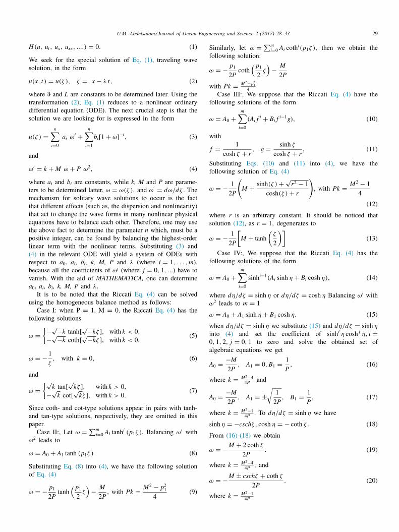
Fig. 3. Three-dimensional profile of the periodic solution [given by Eq. (55) ] for a 0 = 3 . 1 , k = 0. 5 , λ = 0. 1 and B = 3 .
− 10 − 5 0 5 10x
− 10
− 5
0
5
10
t
− 50
0
50
u
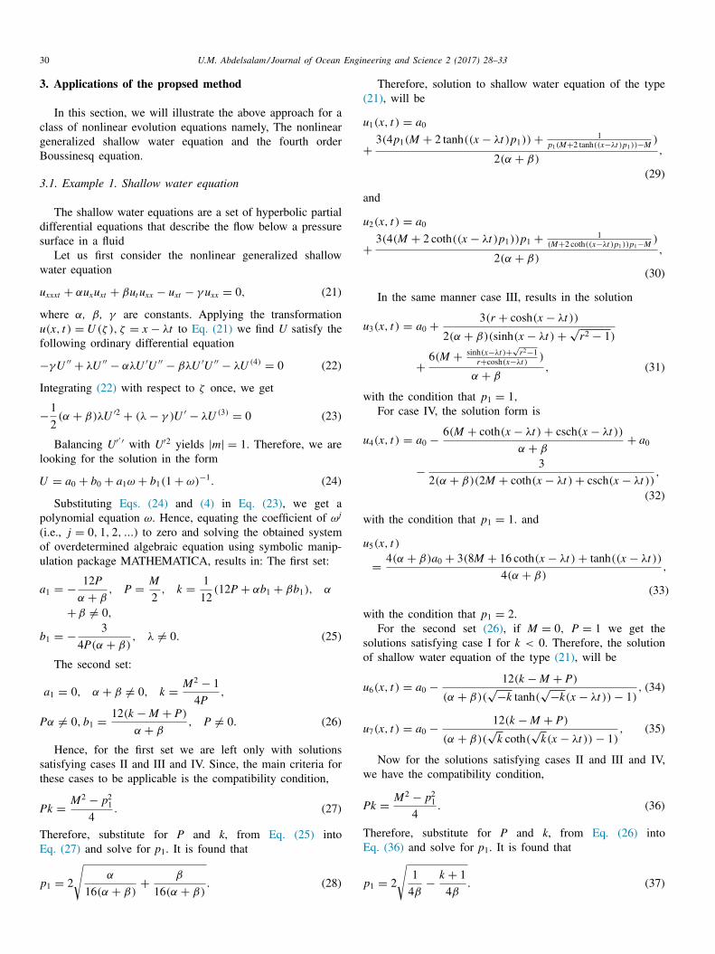
Fig. 4. Three-dimensional profile of the explosive/blowup pulse [given by Eq. (58) ] for the same parameters as in Fig. 3 .
p
f
b
s
i
h
a
4
p
nw
g
B
o
R
[[[
[[[
[[[
[[[[[
eriodical solutions develop a singularity at a finite point, i.e.or any fixed t = t 0 there exist an x 0 at which these solutionslow up , see Fig. 3 , while solutions (31) and (58) are explo-ive/blowup solutions as depicted in Fig. 4 . and the solutions
n (59) is a rational-type solution. Rational solutions may beelpful to explain certain physical phenomena. The solutionsre useful in physical aspects and applied mathematics.
. Conclusions
An extended homogeneous balance method with com-uterized symbolic computation is developed to deal withonlinear partial differential equations (PDEs). Traveling
ave solutions were formally derived for the nonlineareneralized shallow water equation and The fourth orderoussinesq equation. This method can be also applied tother nonlinear evolution equations.
eferences
[1] P.G. Drazin , R.S. Johnson , Solitons: An Introduction, Cambridge Uni-versity Press, Cambridge, 1989 .
[3] R. Hirota , R. Bullough , P. Caudrey , in: Backlund Transformations,Springer, Berlin, 1980, pp. 1157–1175 .
[4] A.M. Wazwaz , J. Ocean Eng. Sci. 1 (2016) 18118 . [5] W. Malfliet , Am. J. Phys. 60 (1992) 650–654 . [6] Y.T. Gao , B. Tian , Comput. Math. Appl. 33 (1997) 115–118 . [7] E. Fan , Phys. Lett. A 277 (2000) 212–218 . [8] R. Sakthivel , C. Chun , J. Lee , Z. Naturforschung A 65 (2010) 633–640 ;
S.A. Elwakil , S.K. El-Labany , M.A. Zahran , R. Sabry , Chaos Sol. Fract.17 (2003) 121–126 .
[9] S.S. Ray , S. Sahoo , J. Ocean Eng. Sci. 1 (2016) 219–225 . 10] J. Lee , R. Sakthivel , Pramana J. Phys. 81 (2013) 893–909 . 11] A.M. Wazwaz , Appl. Math. Comput. 159 (2004) 559–576 . 12] C. Chun , R. Sakthivel , Comput. Phys. Commun. 181 (2010) 1021–1024 .13] G. Cai , Q. Wang , J. Huang , Int. J. Nonl. Sci. 2 (2006) 122–128 . 14] R. Sabry , M.A. Zahran , E. Fan , Phys. Lett. A 326 (2004) 93 . 15] W.M. Moslem , U.M. Abdelsalam , R. Sabry , P.K. Shukla , New J. Phys.
12 (2010) 073010 . 16] M.L. Wang , X. Li , J. Zhang , Phys. Lett. A 372 (2008) 417–421 . 17] A. Bekir , Phys. Lett. A 372 (19) (2008) 3400–3406 . 18] U.M. Abdelsalam , M. Selim , J. Plasma Phys. 79 (2013) 163–168 ;
M.M. Selim , U.M. Abdelsalam , Astro. Space Sci. 353 (2) (2014)535–542 .
19] M.L. Wang , Phys. Lett. A 199 (1995) 169–172 . 20] M.L. Wang , Phys. Lett. A 216 (1996) 67–75 . 21] E.G. Fan , H.Q. Zhang , Phys. Lett. A 245 (1998) 389–392 . 22] L. Yang , Z. Zhu , Y. Wang , Phys. Lett. A 260 (1999) 55–59 . 23] E.G. Fan , Phys. Lett. A 265 (2000) 353–357 .


![Deriving one dimensional shallow water equations from mass ...equations over depth Fig.2, a schematic view of hydraulic jump [10]. 2. Derivation of Navier-Stokes equations for shallow](https://static.documents.pub/doc/80x56/5e91493e68a8585a8017f546/deriving-one-dimensional-shallow-water-equations-from-mass-equations-over-depth.jpg)


