This document has been made available through Treasures at UT Dallas, a service of the Eugene McDermott Library. Please contact [email protected]for additional information. Treasures at UT Dallas Eric Jonsson School of Engineering and Computer Science 6-2009 Finding a Simple Path with Multiple Must- include Nodes Hars Vardham, et al. Follow this and additional works at: http:// http://libtreasures.utdallas.edu/xmlui/handle/10735.1/2637
Transcript
This document has been made available through Treasures at UT Dallas, a service of the Eugene McDermott Library. Please contact [email protected] for additional information.
Treasures at UT Dallas
Eric Jonsson School of Engineering and Computer Science
6-2009
Finding a Simple Path with Multiple Must-include Nodes Hars Vardham, et al.
Follow this and additional works at: http:// http://libtreasures.utdallas.edu/xmlui/handle/10735.1/2637
Finding a Simple Pathwith Multiple Must-include Nodes
Technical Report UTD/EE/2/2009
June 2009
Hars Vardhan∗, Shreejith Billenahalli∗, Wanjun Huang∗, Miguel Razo∗, Arularasi Sivasankaran∗,Limin Tang∗, Paolo Monti†, Marco Tacca∗, and Andrea Fumagalli∗
∗Open Networking Advance Research (OpNeAR) LabErik Jonsson School of Engineering and Computer ScienceThe University of Texas at Dallas, Richardson, TX, USA
This document presents an algorithm to find a simple path in the given network with multiple must-includenodes. The problem of finding a simple path with only one must-include node can be solved in polynomial timeusing lower bound max-flow approach. However, including multiple nodes in the path has been shown to be aNP-Complete. This problem may arise in network areas such as forcing the route to go through particular nodes,which have wavelength converter (optical), have monitoring provision (telecom), have gateway functions (in OSPF)or are base stations (in MANET). Also, network standards allow loose definition of routing by requiring one ormore nodes to be in the routing of Link State Packet. In this document, a heuristic algorithm is described to find asimple path between a pair of terminals, which has constraint to pass through a certain set of other nodes.
The algorithm is comprised into two main steps: (1) considering a pair of nodes in sequence from source todestination as a segment and then computing candidate paths between each segment, and (2) combining paths, onefrom each segment, in order to make simple path from source to destination. The max-flow approach is used to findcandidate paths, a which provides maximum number of edge disjoint paths for individual segments. The secondstep of the algorithm uses backtracking algorithm for combining paths. The time complexity of the first step of thealgorithm is O(k|V ||E|2), where k is the number of must-include nodes. The time complexity of step (2) dependsupon total number of candidate paths which are not touching any one of the candidates of other segments. So, theworse case time complexity of step (2) is O(λk), where λ is the maximum nodal degree of the network. However, weshow that step (2) has minimal effect on the algorithm and it does not grow exponentially with k in this application.Later, we also show that initial re-ordering of the given sequence of must-include nodes can improve the result. Theexperimental results show that the algorithm is successful in computing near optimal path in reasonable time.keywords: constrained path computation, graph theory, heuristic algorithm, max flow, network route.
I. INTRODUCTION
Network standards [1] [2] [3] allow loose definition of routing by requiring one or more nodes to be in the route
of Link State Packet. This problem may arise in various networking areas such as optical networks, OSPF (Open
Shortest Path First) protocol, telecommunication networks, and MANET (Mobile ad-hoc networks). For example,
the optical network routing may require the route to include some specific nodes, which are wavelength converter or
amplifier/regenerator enabled. OSPF network may have some of the nodes to act as gateways across the subnetwork,
which must be included in the path when source and destination are multiple subnet apart. In telecommunication
network, routing of the traffic may be forced to go through specific nodes that have traffic monitoring capability.
MANET often require routes through some designated nodes, which are directly connected to a base station.
The problem of including only one node in the computation of a simple path is polynomial time solvable using,
for example lower bound max-flow [4], as briefly described next. The lower bound max-flow algorithm computes a
flow, which must include all the edges that have a positive (> 0) lower bound value. If only one edge has a positive
lower bound, the flow computed by the algorithm can be used to build a simple path, which includes such edge.
The “edge” instance of the problem can be transformed into its “node” equivalent by first splitting the include-node
into two half-nodes, i.e., n1 and n2. All incoming edges to the original node converge to n1. All outgoing edges of
the original node emerge from n2. A directed edge el from n1 to n2 is added with a positive lower bound value.
All other (original) edges of the network have zero lower bound. Now, applying the lower bound max-flow [5]
algorithm to this flow network, a feasible flow from source to destination can be found such that el is included in
at least one of the (flow) augmenting paths. Then on merging n1 and n2 the simple path can be traced. The lower
bound max-flow technique cannot be successfully applied to 2 or more include nodes, as there is not a guarantee
that the same augmenting path in the flow algorithm contains all of them at once. Hence, it is not possible to trace
out a simple path with all of the must-include nodes.
The shortest path with multiple must-include nodes can be seen as a more general case of the well known
traveling salesman path (TSP) problem, which is NP-complete1. Instead of traveling all nodes as in the original
TSP, this problem requires to travel only a subset of the nodes from source to destination. This problem can be
solved by brute-force method of complete enumeration of all the possible paths and then choosing the best path
which contains all must-include nodes. Akin to the TSP problem, the number of enumerations in the problem is
exceedingly large [8]. Given a network of n(= |V |) nodes, the number of possible such tours is exponential, or
more precisely O(n!). On the other hand, if a path is given from source to destination then it can be verified in
polynomial time whether it includes all the nodes of I . Given a path P , presence of any loop in P can be checked
1The TSP problem and its variations have been addressed by a number of papers in the literature, e.g., [6] [7].
2
in O(|V |) time. Simultaneously, it can also be verified that P has all must-include nodes in it. Hence, this problem
belongs to the class of NP-complete problems.
In this document, a heuristic algorithm is proposed to compute a simple path which contains a given ordered
set of must-include nodes, i.e., set I . The algorithm’s primary objective is to find at least one simple path, which
satisfies the must-include routing constraint. However, the nature of the algorithm itself leads to finding near shortest
path solutions. The algorithm comprises two main steps: (1) considering each pair of consecutive nodes in I to
represent a segment of the entire end-to-end path from source to destination, and then computing candidate paths
for each segment; (2) Concatenate segment paths, one from each segment, in order to make a simple path from
source to destination. We use the max-flow [9] approach to find candidate paths for each segment, which yields
the maximum number of edge-disjoint paths for each individual segment. The time complexity of this first step of
the algorithm is O(k|V ||E|2), where |V | and |E| are the number of nodes and edges in the network and k is the
size of set I . The second step of the algorithm uses a backtracking algorithm for combining segment paths and
may even find more than one end-to-end edge-disjoint paths, which contain all of the nodes in I . The worse case
complexity of the backtracking algorithm is O(λk), where λ is the maximum degree of the node in the network.
However, in practice, the run time of this second step is affected by the number of pairs of candidate paths across
segments, which are not disjoint2 . Though the backtracking algorithm is exponential in terms of k, the number
of such disjoint path pairs decreases with increasing value of kn . Consequently, step (2) has minimal effect on the
algorithm’s run time and it stays reasonably low even at large values of k.
As intuition suggests, the order of the nodes in set I may significantly affect the algorithm outcome. Two cases
are considered in this paper. In one case, the node order in I is randomly given, and cannot be changed. In the
other case, the nodes in I can be re-ordered based on depth first traversal before running the proposed algorithm.
Experimental results presented in the document indicate that the proposed algorithm is able to find a simple path
with must-include nodes and requires reasonable run time in most cases. In addition, we quantify the performance
gain obtainable when set I can be re-ordered based on depth first traversal.
II. ALGORITHM DESCRIPTION
In this section, the formal definition of the routing problem constrained to set I — the set of must-include nodes
— is given, followed by the detailed description of the algorithm proposed to solve the problem. Finally, a simple
algorithm is described, which favorably re-orders the set of nodes in I to improve the final outcome.
Given a directed graph G = (V,E) and a set I ⊂ V , the objective is to find a simple path P from source s ∈ V
to destination t ∈ V . The nodes in set I must be present in P . Let k = |I| be the number of nodes in set I . Let
2Two paths are disjoint to each other if together, they are not making any loop
3
ui ∈ I , where i = 1, 2, 3...k, be the nodes in I . Then, P must have the following property:
∀ui ∈ I =⇒ ui ∈ P; i = 1, 2, 3....k (1)
Simple solutions to this problem can be found in two special cases. If k = 1, the problem can be solved using lower
bound max-flow algorithm [4]. If the constraint of finding simple path is removed, then the problem is reduced
to computing shortest path between every pair of nodes (or segment) (s, u1), (u1, u2) . . . , (uk, t) along P . The
concatenation of the segment shortest paths forms an end-to-end path which may not be simple, i.e., it may contain
loops. However, in general, i.e., when k ≥ 2 and the path must be simple, the problem is NP-Complete. In order
to prove this, the proof of NP-completeness of TSP problem can be extended which is shown in Section I.
One can obtain a straightforward solution to the problem by directly using K-shortest path algorithm [10]. The
K-shortest path algorithm can be called repeatedly by gradually increasing the value of K starting from K = k, till
“equation (1)” is satisfied. Though this approach results in shortest (optimal) path, the required value of K may be
large in most cases, thus making the solution impractical. (In Section III the K-shortest path approach is applied
to a small network and a small size of I to offer an optimum result to compare our heuristic against in terms of
hop count.)
Further, the set of must-include nodes I may be given as an ordered set. In this case, P must have the following
additional property. Let π(x) denote the index of node x in P , then
∀ui, uj ∈ I ∧ i < j =⇒ π(ui) < π(uj) (2)
Adding constraint given by “equation (2)” does not change the hardness of the problem.
We first address the problem with both of the constraints given in “equation (1)” and “equation (2)”. The
algorithm follows divide and conquer approach. Firstly, it computes multiple candidate paths for each individual
segment. Then, combining paths, one from each segments such that they do not form a loop, gives the solution.
Let I = {u1, u2, u3.....uk}, then we define segments segi, i = 0, 1, 2..k as follows: seg0 = (s, u1), seg1 =
(u1, u2), seg2 = (u2, u3) .... segk = (uk, t). Conversely, we can say s = seg0.first, u1 = seg0.second =
seg1.first, .... uk = segk.first = segk−1.second. So, given k must-include nodes, there are k + 1 segments.
Also, Pi is defined as a collection of all edge-disjoint candidate paths for segi. Pij represents jth path (starting
from index 0) of Pi. The algorithm uses two procedures: findDisjointPaths(segi) and combinePaths(m, P , P). The
procedure findDisjointPaths(segi) computes all edge-disjoint paths Pi for segi. Edge-disjoint paths for each segment
are computed by setting the capacity of all edges in the graph G(V,E) to 1. Then, maximum flow from v1 to v2 is
computed using max-flow algorithm, where v1 = segi.first, v2 = segi.second. Now, by using depth-first search
4
(DFS) of nodes from v1 to v2 along only those edges which has flow > 0, all disjoint paths of Pi for segi can be
traced one by one. The procedure findDisjointPaths(segl) is formally described in Algorithm 1 which returns set
of paths Pi for segi. Pi is sorted according to ascending order of the length of the path.
Algorithm 1 : findDisjointPaths(segl)1: v1 ← segl.first2: v2 ← segl.second3: for all ui ∈ I : ui 6= v1 ∧ ui 6= v2 do4: ∀e : edge e passing through node ui; capacity(e) = 05: end for6: compute flows F =
⋃f(i, j) ∀ ui, uj ∈ V in order to maximize the flow between v1 and v2
7: m← 08: while ∃i, j : f(i, j) > 0 do9: ux ← v1
10: Plm ← {ux} // {Plm is a vector of nodes}11: repeat12: if ∃uy : f(x, y) > 0 then13: Plm ← Plm + {uy} // {push-back an element}14: ux ← uy15: f(x, y)← f(x, y)− 116: end if17: until ux = v218: m← m+ 119: end while20: return Pl
This procedure is called for all segments (segi; i = 0, 1, 2...k) in order to compute candidate paths P . Since max-
flow algorithm is used for path computation, all paths within Pi are edge-disjoint. The step 3-5 of the Algorithm 1
ensures that the paths for segi do not touch any other include-node that is not belonging to segi. A candidate
path which traverses some include-node other than nodes of its corresponding segment will never lead to a simple
path. By removing those nodes (temporarily) each time before running max-flow algorithm, such possibilities can
be avoided. Additional effect of temporarily removing nodes results in a network graph of n − k nodes. So, the
max-flow algorithm runs on the network of only n − k nodes instead of n. Step 6 of the Algorithm 1 computes
maximum flow between the segment, and step 8-19 trace all edge disjoint paths for the segment.
The another procedure combinePaths(m, P , P) uses output P of the Algorithm 1 in order to compute desired
path from s to t. The procedure combinePaths(m, P , P) computes a simple path by combining paths, one from
each of the segments. The procedure is defined formally in Algorithm 2. The resultant path P is a path (sequence
of nodes) in the order it is added.
Initially, P is empty. Also, the information about current segment is passed as first parameter of the procedure. This
is a recursive procedure which should be initially invoked like combinePaths(0,P ,φ). The procedure combines paths
5
Algorithm 2 combinePaths(m, P , P)1: if m > k then2: return 13: end if4: ret← −15: for all path p ∈ Pm do6: if ∃ p : p ∪ P not making a loop then7: P.push back(p)8: ret← combinePaths(m+ 1, P , P)9: if ret = −1 then
10: P.pop back() // {Undone last step}11: end if12: end if13: end for14: return ret
from each of the segments to make a simple path. Step 1-3 ensures the successful termination of the Algorithm 2.
Step 7-8 selects and concatenate a possible sub-path (not making loop with previously selected sub-paths) from
current segment and proceed toward next segment. In steps 9-10, previous concatenation of a sub-path is undone
and the for-loop (step 5) looks for another possible sub-path for the current segment. On success, Algorithm 2
returns 1, and −1 otherwise.
It is possible that there are more than one possible paths from s to t, all of them are satisfying the constraints given
in “equation(1)” and “equation(2)”. On removing all paths from candidate set, which are successfully combined in
the previous steps, process of combining paths can be repeated until no further simple path is found. For computing
more than one such edge-disjoint paths, the procedure combinePaths(m, P , P) should be called repeatedly after
removing all sub-paths (Pij) used in previous rounds from P .
Algorithm 1 is using max-flow approach to compute all possible edge-disjoint paths for each of the segments. The
max-flow algorithm is called for each segment. So, the total time complexity of the Algorithm 1 is O(k|V ||E|2),
where k = |I| is the number of include nodes in the given network graph G(V,E). The max-flow algorithm used
in our implementation is given by Edmonds-Karp [9] which has the time complexity of O(|V ||E|2). However, our
algorithm is independent of a particular algorithm used to compute the maximum flow between a pair of terminals.
The next procedure described in Algorithm 2 is a backtracking algorithm that iterates through all possible cases
until it finds a solution which turns into k multiplications of number of edge-disjoint paths in each of the segments.
Here, number of paths for each segment is bounded by the maximum nodal degree(λ) of the graph G. Hence the
worse case complexity of Algorithm 2 is O(λk).
The procedure in Algorithm 2 can be shown to be a k-clique problem. In order to show that, we will create a
6
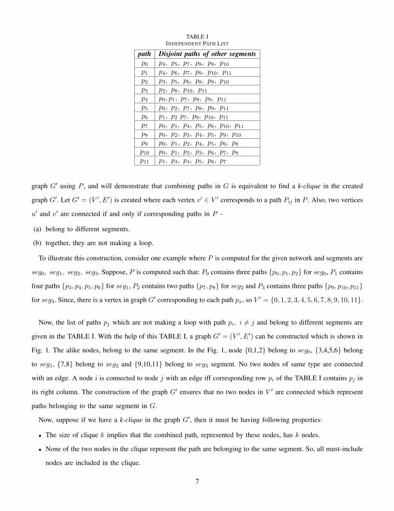
TABLE IINDEPENDENT PATH LIST
path Disjoint paths of other segmentsp0 p4, p5, p7, p8, p9, p10
p1 p4, p6, p7, p9, p10, p11
p2 p3, p5, p6, p8, p9, p10
p3 p2, p8, p10, p11
p4 p0, p1, p7, p8, p9, p11
p5 p0, p2, p7, p8, p9, p11
p6 p1, p2 p7, p9, p10, p11
p7 p0, p1, p4, p5, p6, p10, p11
p8 p0, p2, p3, p4, p5, p9, p10
p9 p0, p1, p2, p4, p5, p6, p8
p10 p0, p1, p2, p3, p6, p7, p8
p11 p1, p3, p4, p5, p6, p7
graph G′ using P , and will demonstrate that combining paths in G is equivalent to find a k-clique in the created
graph G′. Let G′ = (V ′, E′) is created where each vertex v′ ∈ V ′ corresponds to a path Pij in P . Also, two vertices
u′ and v′ are connected if and only if corresponding paths in P -
(a) belong to different segments.
(b) together, they are not making a loop.
To illustrate this construction, consider one example where P is computed for the given network and segments are
seg0, seg1, seg2, seg3. Suppose, P is computed such that: P0 contains three paths {p0, p1, p2} for seg0, P1 contains
four paths {p3, p4, p5, p6} for seg1, P2 contains two paths {p7, p8} for seg2 and P3 contains three paths {p9, p10, p11}
for seg3. Since, there is a vertex in graph G′ corresponding to each path px, so V ′ = {0, 1, 2, 3, 4, 5, 6, 7, 8, 9, 10, 11}.
Now, the list of paths pj which are not making a loop with path pi, i 6= j and belong to different segments are
given in the TABLE I. With the help of this TABLE I, a graph G′ = (V ′, E′) can be constructed which is shown in
Fig. 1. The alike nodes, belong to the same segment. In the Fig. 1, node {0,1,2} belong to seg0, {3,4,5,6} belong
to seg1, {7,8} belong to seg2 and {9,10,11} belong to seg3 segment. No two nodes of same type are connected
with an edge. A node i is connected to node j with an edge iff corresponding row pi of the TABLE I contains pj in
its right column. The construction of the graph G′ ensures that no two nodes in V ′ are connected which represent
paths belonging to the same segment in G.
Now, suppose if we have a k-clique in the graph G′, then it must be having following properties:
• The size of clique k implies that the combined path, represented by these nodes, has k nodes.
• None of the two nodes in the clique represent the path are belonging to the same segment. So, all must-include
nodes are included in the clique.
7
Fig. 1. The Graph G′ formed by using P
• Since each node in G′ is connected to k− 1 nodes, so each of the corresponding paths all together can make
a desired simple path.
These properties are required and sufficient to combine paths one from each segment to make desired loop less
path. Hence, the problem of combining path is equivalent to the problem of finding k-clique in the induced graph.
Now, we can easily combine all paths represented by nodes in the clique found in order to make a simple path
from source to destination.
The worse case complexity of combining paths depends upon two parameters: λ-maximum nodal degree and
k-number of must-include nodes. However, careful inspection reveals that it depends on the number of candidate
paths in each of the segments. The number of candidate paths for each segment depends upon the ratio λk . Here,
the upper bound on number of paths is λ. More the value of ratio λk is, more number of independent candidate
paths can be found. The reason is, if more number of segments are created, the max-flow will try to maximize the
number (up to λ) of disjoint paths, and so paths belonging to two different segments may be forced to traverse one
or more common nodes. The backtracking algorithm used in Algorithm 2 has capability to prune further iteration
which may lead a path containing two such nodes in G′. On the other hand, if the number of candidate paths in
segments, which are not making loop with others, is very high then the backtracking algorithm terminates early as
it has found the simple path from source to destination. So, effectively the running time of the Algorithm 2 does
not grow exponentially on an average.
Though, the algorithm does not guarantee that the path obtained is the shortest (optimal), the nature of the
8
algorithm results in near shortest possible paths which satisfy the constraint of including given set of nodes. The
max-flow computation uses shortest path for computing augmenting paths [11]. Also, we sort the paths in P
according to the hop-count. Further, the Algorithm 2 traverses nodes of G′, formed by using P , in increasing order
of index of nodes. Hence, the near-shortest possible path will be found first. If the Algorithm 2 is called second
time after removal of all nodes in G′ which belong to previous found paths, the next possible path between s and
t will not be shorter than the previous ones. In order to support this claim, we compared our result for smaller
networks with the results obtained by running K-shortest path algorithm repeatedly with incrementing the value of
K until desired path is obtained. Since the value of K required by K-shortest path algorithm is very large, it is
computationally not possible to get the optimal results for larger networks.
The complete algorithm is formally described in Algorithm 3. The algorithm first make segments from set I and
computes candidate paths using Algorithm 1. The last step of the procedure calls Algorithm 2 repeatedly till all
possible edge-disjoint paths are obtained.
Algorithm 3 incNodePaths(s, t, I ,allPaths)Require: s 6= t
1: j ← 02: for j = 0 to j < I.size() do3: if j = 0 then4: segj ← (s, Ij)5: else6: segj ← (Ij−1, Ij)7: end if8: end for9: segj ← (Ij , t)
10: for j = 0 to j <= I.size() do11: Pj ← findDisjointPaths(segj)12: end for13: loop14: P ← φ15: ret← combinePaths(0, P ,P)16: if ret = 1 then17: allPaths ← P18: P ← P − P19: else20: Break21: end if22: end loop
Further, if the ordering of the must-include given in “equation (2)” can be relaxed, the result of the Algorithm 3
can be improved by re-ordering the nodes in the set I . The re-ordering of nodes in I does not change any part
of the Algorithm 3 or any of the procedures defined in Algorithm 1 and Algorithm 2. It only possibly change the
9
relative ordering of the include nodes in the desired path. This pre-computation step can be done before calling the
Algorithm 3.
The re-ordering of include nodes can be done using simple algorithm such as depth first traversal. Let the set I ′
is the outcome of this process. Starting depth first traversal from s, suppose the node that is traversed first among
I is x1, then it should be placed first in say I ′. Now, restarting depth first traversal from x1, let the node x2 is
traversed first among I − I ′ then x2 should be placed next in I ′. Repeating the process until I − I ′ = φ results
in I ′ which contains all element of I but may be in different order. The new set I ′ of must-include nodes can be
used instead of I in Algorithm 3.
The motivation of Algorithm 1 is to find maximum number of candidates for each of the segments such that
each of the candidates is sharing the least number (0) of intermediate nodes with other candidates. And, the idea
behind re-arranging the order of must-include nodes using depth first traversal is to avoid making a segment with
nodes that are far apart. If the two nodes of the segment is nearer, the number of hops in the candidate paths for
the segment is lesser. Hence, the possibility of interfering of a candidate path with other candidates is decreased
and path combining process in Algorithm 2 becomes more successful.
The effect of re-ordering the nodes in I is illustrated with a simple example. Let, for a given source s and
destination t in network graph G, the set of include nodes I = {I1, I2}. In Fig. 2, s, t, I1 and I2 are shown
in bigger circle along with other nodes in smaller circle. Now, segments are formed by using set I , which are
Fig. 2. Candidate paths without re-ordering I in G.
seg0 = (s, I1), seg1 = (I1, I2) and seg2 = (I2, t). The computation of candidate paths for each segment results
into following:
P00 = [s, 1, 2, 3, I1]
P10 = [I1, 4, I2]
P20 = [I2, 3, 5, 6, t].
It can be seen that node 3 is forced to be used in P00 and P20 which are candidate paths of seg0 and seg2
correspondingly and therefore, they can not make a simple path together. On the other hand, if we consider re-
10
Fig. 3. Candidate paths after re-ordering I .
arranged elements of set I = {I2, I1}, then candidate paths shown in Fig. 3 would be as following:
P00 = [s, 1, I2]
P10 = [I2, 4, I1]
P20 = [I1, 5, 6, t].
In this case, paths P00, P10 and P20 can be combined in order to find a simple path from s to t, which increases
the overall performance of the proposed algorithm.
Experimental studies are done for both of the above scenarios individually and results are discussed in the next
section.
III. EXPERIMENTAL RESULTS
Simulation experiments are carried out on several instances of input parameters to verify the effectiveness of the
proposed algorithm. The input parameters are the topology layout and the list of traffic requests, each defined by
both source-destination pair and set I (the set of must-include nodes). Network topologies are generated randomly
keeping the number of nodes at n = 50 3 and varying the average nodal degree (λ). The nodes are placed within
a defined square area. An edge between two nodes is added with a probability that is inversely proportional to
the geographical (euclidean) distance between the two nodes4. In practice, the distance between any two edge-
connected nodes is bounded from above by some value. The source and destination of each request (s and t) are
chosen randomly in the topology. Similarly, k must-include nodes are chosen randomly in the topology, excluding
both s and t as possible choices. For each tuple (n, λ, k), 100 requests are created and their average results are
presented.
The performance parameters computed in the experiments are:
- Nsucc: The number of times the experiment finds at least one simple path.
3For scalability test, we have run additional experiments for larger networks up to n = 1000 and up to λ = 100 with similar results.4There are many physical properties of network devices and equipments that may limit the maximum link length, e.g., loss of signal
strength, signal distortion.
11
- Davg : The average number of edge disjoint paths found per request.
- Texp : Total experiment run time.
Nsucc represents the number of instances out of 100 for which the algorithm is able to find at least one path from
s to t that satisfies the must-include node constraint given in “equation (1)”. Davg represents the average number
of edge-disjoint paths that are found per request, accounting for all 100 experiments. Texp represents the average
execution time of the experiment for all 100 requests. Texp is the sum of the run time required by both Algorithm 1
and Algorithm 2. The suffix (W) denotes the result of the experiment without the reordering of I . The suffix (R)
denotes the result of the experiment with the reordering of I . All of the experiments are conducted on the same
hardware and software platform. The complete result is shown in the table II. In the following paragraphs, each of
the parameters are discussed one by one.
First, parameter Nsucc is analyzed with respect to the average nodal degree (λ) as well as with respect to the
number of include nodes (k). The study of parameter Nsucc is shown in Figs. 4 and 5. As λ increases, Nsucc increases
0 5 10 15 20 25 30 35 400
10
20
30
40
50
60
70
80
90
100
Nodal degree (λ)
N succ
Nsucc
(W)
Nsucc
(R)
Fig. 4. Nsucc vs nodal degree (λ): n = 50, k = 20
if k remains constant (Figure 4). Nsucc decreases with increasing values of k (Figure 5). These plots support the
earlier claim that the availability of more disjoint candidate paths for every segment favors the success rate of the
algorithm. Indeed, if we increase the value of λ, keeping all other parameters constant, max-flow algorithm tends
to find more disjoint candidate paths for each segment. Hence, results tend to improve with increasing values of λ.
Also, increasing the ratio kn (by increasing k in this document), candidate paths computed for different segments
are more likely to share some nodes in set N − I . Consequently, it becomes increasingly difficult for the algorithm
to find a loop-less path from s to t. Dependency of Davg on λ (k) is shown in Figs. 6 and 7. Parameter Davg
follows the same trend of parameter Nsucc. In Figure 6 the gap between (W) and (R) decreases for increasing
values of nodal degree, as the relative large number of include nodes (k = 20) limits the probability of finding
additional simple paths even when reordering set I .