Disclaimer: The views expressed are those of the author(s) and do notnecessarily reflect the views of the New Zealand Treasury. The Treasurytakes no responsibility for any errors or omissions in, or for thecorrectness of, the information contained in these working papers.

TREASURY WORKING PAPER

99/2

Private and Public Returns toInvestments in Secondary and

Higher Education in New ZealandOver Time: 1981-1996

Sholeh Maani*(Contract to New Zealand Treasury, managed by Ron Crawford)

ABSTRACT

With significant increases in the demand for new skills and participation inhigher education in New Zealand since the 1980s, and the introduction ofeconomic reforms toward market liberalisation since the mid 1980s, anexamination of income returns to investments in higher education has been ofsignificant interest. This study utilises micro level data from the New ZealandCensus for the years 1996, 1991, 1986 and 1981 to examine the market returnsto post-compulsory secondary and tertiary education for males and females.Internal rate of return estimations of private and public returns to education, andeconometric modelling with formal stability tests of changes in returns over timeare employed to examine the magnitude and changes in returns to highereducation over the fifteen year period. The period of the study is of interest,spanning the period before and after the introduction of the first set of reforms in1984, and labour market reforms in 1991. The results show strong support foran increase in the returns to tertiary education in the 1981-1991 period, and astabilisation of results for males and a relative decline in the returns for femalessince 1991.

*Department of Economics, University of Auckland, Auckland, New Zealand. E-mail: s.maani@auckland.ac.nz

I. Introduction

This study provides a 1996 analysis of the private and public returns to investments in

higher education in New Zealand. The analysis utilises micro level data from the 1996

Census of New Zealand Population and Dwellings. Utilising the two conventional

methods of ‘earnings functions’ and ‘internal rates of return’, it provides estimates of

personal and public returns to investments in post-compulsory education. The study

examines returns to secondary and higher education for males and females and it provides

comparable estimates over the four census years of 1981 through 1996. The analysis

extends earlier research for New Zealand over the 1981-1991 census years (Maani, 1994,

1996a, 1996b, 1997).

The economic reforms in New Zealand, the salient features of which were privatisation

and market liberalisation, have attracted much international interest in recent years as a

major economic case study. Now with the passage of more than a decade since the

introduction of the reforms in 1984, studies of the economic impact of the reforms and

economic conditions prior to and after the reforms are emerging in the international

literature. The purpose of this study is to examine how relative income levels, and in

particular the income returns to post-compulsory and higher education (education beyond

age 16) have changed over the 1981-1996 period, spanning the period prior to and after

the introduction of the reforms in 1984.

Major changes in the structure of the New Zealand economy, including market

liberalisation over the past decade, have prompted a need for new skills, resulting in

significant increases in participation in higher education. In addition, the economic

reforms since 1984, skill shortages in new areas of economic activity, and increased

pressures for international competitiveness have guided income returns to various skill

levels, resulting in increased participation rates in higher education in the late 1980s and

the 1990s.1 Therefore, in examining the returns to investments in higher education since

* I would like to thank Statistics New Zealand for assistance with data analysis,

referees for insightful comments, and Adam Warner at Auckland University forresearch assistance.

2

1981 and in 1996, both demand and supply forces are expected to have contributed to

changes in education income premiums as observed in comparison with the three earlier

years.

The link between educational qualifications and income levels has been of interest for a

number of reasons, including the income distribution effects of educational investments,

and the international literature in this area is vast and growing. These studies have

generally utilised cross section analyses for one time period (e. g. Miller, 1982, and

McNabb and Richardson, 1989 for Australia; Ogilvy, 1970 and Hunt and Hicks, 1985 for

New Zealand; Demetriades and Psacharopoulos, 1987 for Cyprus; Rumberger, 1987, and

Raymond and Sesnowitz, 1983 for the U.S.; and Vaillancourt, 1986 for Canada).2 The

analysis of rates of return to education that are comparable over time has, however, been

addressed in relatively few studies. For example, Miller (1984) and Chia (1990) have

examined changes in returns to higher education in Australia over time, while Ryoo

(1988), Wilson (1985), and Psacharopoulos (1994) provide international evidence on this

question.

Earlier research for New Zealand utilising 1981, 1986 and 1991 census data (Maani,

1994, 1997) has shown that the returns to higher education are positive and significant in

New Zealand. Moreover, the results have strongly indicated that consistent with the

significant increases in participation rates, market rewards to education have been

significant and increasing during the 1981-1991 decade.

Three features of the 1996 analysis compared to the earlier census years are noteworthy.

First, a greater proportion of the New Zealand population has engaged in higher

education since 1991, and the effect of this increased supply on the returns to higher

education in 1996 is of interest. Second, fees, which were not a feature of tertiary

decisions prior to 1991, have come to play a much more significant role in the financing

1 For a detailed discussion of the New Zealand reforms the reader may refer to Evans, et.

al. (1996), and Siverstone and Bollard (1996).

2 Schultz (1988) provides an overview of relevant issues. Tan (1989) providesevidence for the Phillipines, Anderson (1988) for El Salvador, and Jamison andVan der Gaag (1987) provide estimates for the People’s Republic of China.

3

of higher education by the middle part of the decade. Finally, and importantly, the

composition of the New Zealand population has been significantly affected by the

changes in New Zealand immigration law and the resulting immigration trends since

1991, which have increased the relative number of immigrants with higher education and

from non-English speaking countries. These features are considered in the 1996

analysis.

The two methods of ‘earnings-function’ regression analysis and the Internal Rates of

Return (IRR) methods are used in estimating income returns to higher education. The

earnings function method uses semi-logarithmic functions and binary variables for

different education levels, utilising individual level data. In the internal rate of return

model, in turn, (see Psacharopoulos, 1981 and 1994, the ‘elaborate method’) age income

profiles are estimated based on regression models. The IRR models utilise individual

level data to estimate the internal rates of return at which (a) the sum of the net present

values of expected lifetime incomes, and (b) foregone earnings and direct expenses

during the years of education, are equated.

The two methods are complementary. Regression analysis, generally favoured for its

convenience, provides estimates of private market returns to various educational levels.

This method is also favoured for allowing formal stability tests of returns to educational

degrees over time, as employed here for the test of potential change in income returns to

education over the four census years. The regression method, however, does not

incorporate direct costs of education such as fees. The ‘internal rate of return’ method, in

turn, has the advantage of incorporating both the direct costs of education and the lifetime

nature of returns to education, where the costs include foregone earnings and out of

pocket payments such as fees. The social rates of return are further estimated by the

‘internal rate of return’ method, which incorporates the private and public costs of

education. Computationally, the IRR method estimates are expected to result in lower

rates of return than the regression method, when foregone earnings are significant. The

complementary relationship of these methods is expected to present a more

comprehensive set of results for this analysis.

In the next section the data set and the characteristics of the sample are discussed. In

section III returns to secondary and tertiary education in 1996 are examined, based on

4

‘earnings-function’ regression analysis of income levels, and comparisons are made to

results for the census years of 1981, 1986 and 1991. In Section IV the analysis of returns

to education using the Internal Rate of Return (IRR) method is presented for 1996, and

over time. This analysis is extended to incorporate the personal financing of tertiary

education. In Section V, the IRR method is further employed to incorporate government

expenditures on education in the analysis of the public returns to education, based on the

1996 census and in comparison to the three earlier census years. This analysis

incorporates the effect of fees in 1996. Finally, conclusions are presented in section VI.

II. Data and Characteristics of Sample

The data set for the study consists of the ten percentage sample of the New Zealand

Census of Population and Dwellings for 1996 (in conjunction with 10% data sets from

1981, 1986 and 1991), and the samples consist of those in the age group 16-65. Of the

various New Zealand data sets, the census utilised provides the most suitable option by

representing the overall New Zealand population, providing comparable information over

time, information on educational qualifications and sufficient observations at each

education level.

The census provides information on an individual's highest educational qualifications,

making a distinction between the levels of School Certificate (year 11), Sixth Form

Certificate (Year 12)3 , Bursary (Year 13), Post-School Diploma, University Bachelor's

degree, and Postgraduate degrees, in comparison to the control group with no secondary

school qualifications, providing useful education levels for the analysis. Since primary

education is nearly universal in New Zealand, returns to that level of education are not

estimated.

Education is compulsory in New Zealand up to and including the Fifth Form (Year 11,

and age 16), at the end of which nationally administered School Certificate examinations

on up to six subjects are taken. Traditionally, School Certificate has been the highest

educational qualification for at least half of the New Zealand population, and many

3 Sixth Form Certificate refers to the successful completion of examinations at the end of

Year 12.

5

vocational, clerical and trade professions require it.4 The 1996 Census shows that 45.5

per cent of males and 50.2 per cent of females had completed their education at or below

School Certificate level.5

Bursary examinations at the end of the 7th Form (Year 13) were originally designed to

determine merit-based bursary payments to students for studies at university. Admission

to the universities in New Zealand requires Year 13 Bursary, while a number of

polytechnic diplomas and degrees require Sixth Form Certificate (Year 12) or Year 11

School Certificate.6 Nevertheless, some students choose to complete Years 12 or 13 and

then go to polytechnic. As a result, it is noteworthy that the idea of the completion of

secondary school has a wider application in New Zealand by referring to either 12 or 13

years, compared to the 12-year degree in some other countries such as the U.S.

It may be noted that the largest component of income in the census is earnings, but it also

includes unearned income such as interest, rent, and government assistance. To the

extent that higher unearned income is likely to be positively correlated with higher earned

income, the overall effect of the inclusion of these incomes may be to result in rates of

return that are higher than those based on earnings alone. However, the inclusion of

government assistance as a part of income in the census is likely to introduce a negative

correlation and somewhat flatten the age-income profiles, thereby decreasing the above

effect. Despite this characteristic of the data, the New Zealand census provides the most

suitable source of data for the study and since higher education may result in both

increased earned and unearned income, the marginal returns estimated may be considered

4 In New Zealand, schooling starts during a child’s fifth year and continues for

thirteen years—six years of primary school (Junior 1-2, and Standard 1-4), twoyears of intermediate school (Form 1-2) and five years of secondary school (Form3-7). The first year of school (Junior 1) is academically equivalent to the firstgrade in most other countries, so by the time students complete year 13 they areabout 18 years old. In this system, secondary school (Forms 3 through 7) isequivalent to years 9 through 13 of study.

5 In comparison, the 1981 census indicates that, a decade earlier, these measures were 62per cent for males and 69 per cent for females, as shown in Table1.

6 Bursary examinations at the end of the 7th Form are nationally administered examinationson five subjects which determine eligibility for application to various university majors.

6

as the differences in the relative standard of living associated with different education

levels. 7

A summary of the characteristics of the 1996 samples for males and females and in

comparison to the census years 1981-1991 is provided in Table 1. Most significantly, the

statistics in Table 1 show the greater educational attainment of the New Zealand

population over the 1981-1996 period. For example, in 1981 about one half of the sample

(50.1% of males and 54.4% of females) had no school qualifications, but by 1991 this

group had decreased to become approximately one third of the population (e.g. 34.06% of

males and 34.62% of females in 1996).

In addition, education levels have continued to increase between 1991 and 1996,

especially at the tertiary level, for which continued increased attainment levels are

prominent. For example, by 1996, 12.6% of males and 10.0% of females had university

qualifications. This represents a significant increase in tertiary qualifications over the

1981-1996 period from 5.5% of males and 2.7% of females in 1981, or even compared to

7.7% of males and 5.2% of females in 1991.8

A further examination of Table 1 reflects increased labour force participation and

employment rates, and decreased unemployment rates, for both males and females since

1991. In 1996, 80.4% of males and 64.3% of females were employed (compared to

74.5% of males and 56.4% of females in 1991). The 1981-1991 period witnessed

decreasing trends in male employment and participation in the labour force, but

corresponding increases for females. In part, this reflected the changes in labour force

participation patterns, and was also a reflection of increases in the unemployment rates.

In 1981, only 7.4% of males but 51.3% of females were out of the labour force, compared

with 17.3% of males and 37% of females in 1991. In comparison, in 1996, 14.3% of

7 The reader may refer to Psacharopoulos, 1985 and 1994; and Miller, 1982 for a number

of international studies which have used incomes for rates of return estimations.

8 While all education levels show increasing trends, the only exception is theDiploma level which shows decreasing trends in 1996, after a significant increasebetween 1981-1991, (in 1991 one third of the sample had Diplomas (35.5% ofmales and 29.5% of females), compared with 25.8% of males and 22.4% of femalesin 1996).

7

males and 30.0% of females were out of the labour force, which represents a reversal of

the trend for males and a continuation of the trend for females since 1991. In addition,

unemployment rates, which had increased significantly over the 1981-1991 decade, were

lower in 1996 for both males and females.

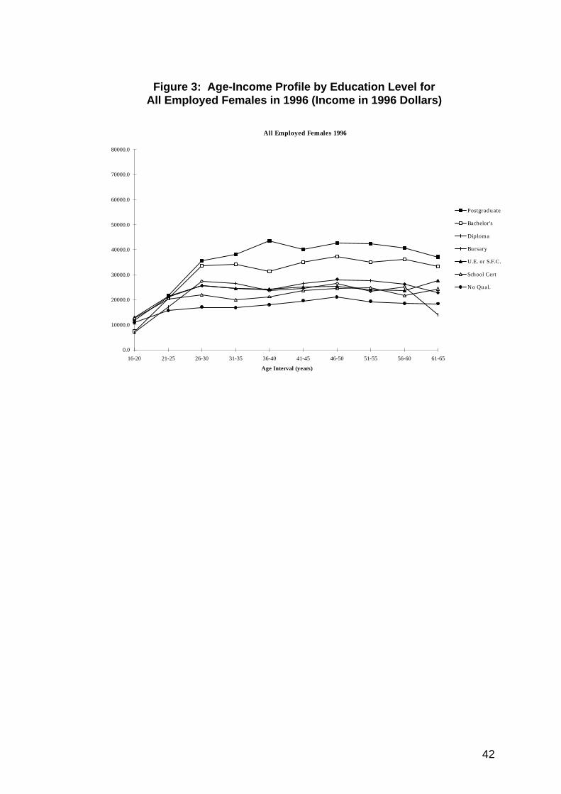
For the analysis of the effect of educational qualifications on income levels, comparisons

of age-income profiles are initially considered in Figures 1 through 4, for the 1996

samples of ‘all employed’ and ‘full-time employed’ males and females. Since sample

characteristics and age-income profiles are significantly different for males and females,

throughout this report separate analyses are presented for the two groups. In addition,

estimates are presented separately for the samples of the employed, and its sub-sample of

the full-time employed, to account for the effect of the hours of work.

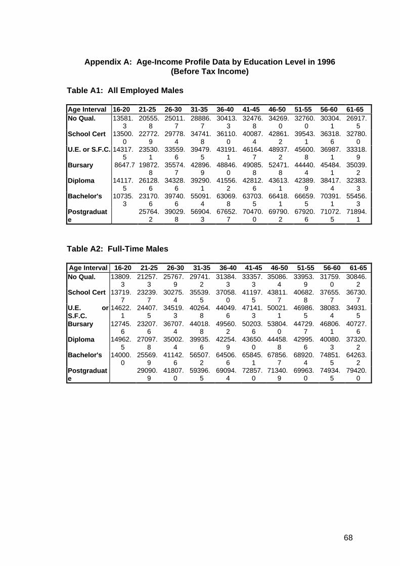
Figures 1-4 show the higher age-income profiles over the life cycle, with higher

educational qualifications in 1996. (The age-income profile data used for creating

Figures 1-4 is also presented in Tables A1- A4 in Appendix A). These figures further

show that, similar to results for the 1981-1991 census years, the incomes profiles for

females are consistently lower and flatter than the profiles for males. Although hours of

work are likely to contribute to this effect, flatter and lower age-income profiles for

females persist for the sample of full-time employed, indicating that other factors, such as

different degrees of on-the-job training and different career paths, are also at work.

The lower overall income levels for females are confirmed when mean income levels by

educational qualifications for males and females are compared in Tables 2 and 3 of the

sample characteristics for the seven educational qualifications in 1996. For example, as

reflected in Table 2, the average annual income for males with Postgraduate

qualifications was $56,059 in 1996, compared to $48,449 for a Bachelor's degree,

$29,829 for School Certificate, and $24,069 for no secondary school qualifications. In

turn, for females the average income for those with Postgraduate qualifications was

$33,645 compared to $26,218 for a Bachelor's degree, $18,048 for School Certificate,

and $13,887 for those with no secondary school qualifications. Similar tables for the four

sub-samples of the ‘all employed’ and ‘full-time employed’ males and females are also

included in Tables B1-B4 in Appendix B.

8

Tables 2 and 3 (and Tables B1-B4 in Appendix B) also provide statistical evidence on

labour market status and personal characteristics of the population by education level.

These measures indicate that there is a clear increase in rates of employment and labour

force participation at higher education levels for females. In comparison to the three

previous census years, the 1996 measures show a continued increasing link between

educational qualifications and employment stability for females over time, as reflected by

employment and unemployment rates for each educational level.9 The increased

participation in the labour force by women with higher education is especially marked.10

In the next section we consider the regression function estimates of the private rates of

return to educational qualifications in 1996, and comparisons will be made to the earlier

census year results.

III. Regression Function Estimates

The model tested is semi-logarithmic with binary variables for educational qualifications

(see for example, Heckman and Polacheck, 1974; and Dougherty and Jimenez, 1991): 11

ln Yi = a + b1School Certi (Year 11)+ b2Sixth Form Certi (Year 12) +b3Bursaryi (Year

13)+ b4Diplomai + b5Bachelor’s Degreei + b6Postgrad. Degreei + b7AGEi + b8AGEi2 +

ui (1)

9 Tables 2 and 3 also indicate that those with Bursary as their highest degree had generally

lower labour force participation rates. Additional statistics based on the census furtherindicate that, for example, 50.5% of the males and 37.8% of the females who were out ofthe labour force in this group were receiving student allowances in 1991.

10 For example, only 14.98% of females with Postgraduate qualifications were not inthe labour force in 1996, compared to 44.72% of the female sample with noqualifications (In 1991 these measures were 15.19% and 50.5% respectively).

11 Heckman and Polachek (1974) and Dougherty and Jimenez (1991) have provided testsof the functional form for the earnings function, and they support the semi-logspecification as the most appropriate of the conventional transformations. Heckman et al.(1996) have provided further evidence that educational degrees have the most effectonce they are completed. This, referred to as the ‘sheepskin effect’, is consistent with thespecification adopted here.

9

where the dependent variable is the natural logarithm of annual income in current dollars.

The model incorporates after-tax measures of income, but estimates based on before-tax

income have also been provided for comparison.12 The excluded educational

qualification level is ‘with no school qualifications’. Variable AGE is included as a

proxy for years of experience in the usual quadratic form.13 In the New Zealand

institutional setting, age has traditionally had prominence in determining earnings as a

measure of overall personal experience. It may be noted that although earnings functions

in the Labour Economics field generally include a number of variables such as race,

family status, union membership, occupation, firm size, etc., in this study the interest is in

the overall rates of return to an educational degree.

The 1996 cross-section results of Model (1) for the two groups of employed, and full-

time employed males, are presented in Table 4 and for females in Table 5. The

differences between the before tax and after tax columns reflect the effect of progressive

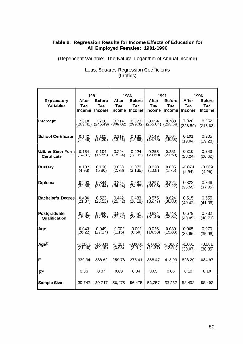
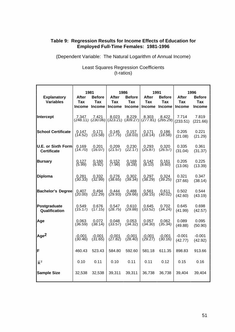
income taxation. Tables 6-9, in turn, provide the above 1996 estimates along with

comparable results for 1981, 1986 and 1991. An extended version of Model (1) above is

also tested with a pooled 10% sample of population over the four census years of 1996,

12 The income information in the New Zealand census (similar to Australia) is reported in 13

categories, based on an annual gross income. The mid-point of these categories hasbeen used as a measure of income throughout the study. The lowest income category inthe census is nil income or loss for which income of zero is designated. The rest of theannual categories were $2,500 or less, $2,501-$5,000, up to $100,000 or more, for whichbased on Statistics New Zealand estimate a mid-point of $130,960 was assumed.

13 The New Zealand Census does not provide information on the actual years of (potential)experience. In the original human capital models, variables for experience andexperience squared are included instead of age, where experience is specified as ‘age -years of schooling - 7’. Using a specification as above instead of age results in returns toeducation that are higher, especially at higher levels of education. Using age comparestwo individuals of the same age but varying years of education and potential jobexperience. Using experience specified as above compares individuals of different agebut similar potential years of work experience. In the New Zealand setting a specificationof ‘Age-years of schooling-5’ is relevant, since school starts at the age of 5. The modelabove was also tested with a specification in which ‘potential years of experience’ wasincluded instead of ‘age’. These results for the years 1981-1996 are presented in TablesC1 and C2 of Appendix C to provide a comparison. As expected, the estimatedcoefficients in the models in relation to potential years of experience are larger, especiallyin relation to tertiary degrees which require more years of study and allowing fewer yearsof work experience in a given age. However, the overall findings of the study regardingrelative returns to degrees, and increases over time remain regardless of thisspecification.

10

1991, 1986 and 1981 for a formal stability test of changes in returns to education over

time. These results are summarised in Tables 10 and 11.

The results in Tables 4 and 5 indicate positive and significant returns to educational

investments in 1996. In addition, the results in Tables 6-9 indicate that the returns to all

qualification levels have increased significantly over the 1981-1996 period, in

comparison to the base group with school qualifications below School Certificate. In

addition, the returns in 1996 have generally stabilised around 1991 levels or increased,

except in the case of a Bachelor’s Degree which has decreased slightly in 1996, in

comparison to 1991 for both males and females. This particular result will be examined

more closely through formal stability tests and further extensions to the model which

adjust for the immigrant composition of the New Zealand population since 1991.

Since model (1) has a semi-logarithmic functional form, the coefficients for continuous

variables, such as age, may be interpreted as a proportional change in income (or a

percentage change when multiplied by 100) due to an increase in age by one year.

Likewise, the coefficients for educational qualifications may be interpreted as the change

in the natural logarithm of income in relation to the education level. However, since the

educational qualification variables are dichotomous (binary) variables, in order to

interpret these coefficients as a percentage gain in income, an adjustment may be used in

relation to the estimated coefficients. The adjustment requires that the anti-logarithm of

the coefficient is taken and the value one is subtracted (see, e.g., Halvorsen and

Palmquist, 1980). For example, the percentage gain in income from School Certificate in

relation to no school qualifications in equation (1) is derived as: gj = [ exp (bj) - 1 ] times

100, where gj reflects the percentage gain relating to this education level, and bj is the

regression coefficient (in Tables 4 - 9). Although for small coefficients below 0.15 or

0.20 the coefficients and adjusted percentages are very similar, for larger coefficients the

adjustments are more significant.

For example, in percentage terms (gj ), the bj coefficient of 0.495 in column seven of

Table 6 for ‘all employed’ males indicates that a Bachelor’s degree was associated with

after-tax incomes that were 64.0 per cent higher than for those with no school

11

qualifications in 1996, compared to 39.8 per cent higher in 1981, and 67.5 per cent higher

in 1991.14

A Postgraduate degree was also associated with an after-tax return of 81.8 per cent (a

coefficient of 0.598) compared to those with no school qualifications in 1996 (79.1 per

cent higher in 1991, and 53.1 per cent in 1981). The marginal percentage return to a

Postgraduate degree over a Bachelor’s degree was in turn higher at 10.8 per cent in 1996

(compared to returns of 6.9 per cent in 1991, and 9.5 per cent in 1981). These results for

1996 further indicate that for the sample of all employed males, the returns to a

Bachelor’s degree decreased slightly since 1991, but that the returns to a Postgraduate

degree have increased since 1991. These results are consistent with the earlier finding

that the returns to higher education for males have been significant and variable over

time.15

The rates of return for females in Tables 5 and 8-9 are generally compatible with the

results for males. The rates of return for females are generally higher than for males for

most educational qualifications in 1996, despite their generally lower earnings. This

result is consistent with the findings for 1981-1991 (Maani, 1996a, 1997), and results

based on the IRR method, of Ogilvy (1970) and Hunt and Hicks (1985) for New Zealand,

and Miller (1982) and Chia (1990) for Australia. These results tend to reflect the relative

advantage of females with educational qualifications over other females engaged in jobs

which require lower qualifications and have lower pay.16

It may also be noted in Tables 4-9 that the regressions for males have higher R2’s than

those for females. This reflects the effect of greater dispersion of hours of work and pay

14 Respectively, with coefficients of 0.335 in column 1 for 1981, and 0.516 in column 5 for 1991.

15 Likewise, compared to the control group, Sixth Form Certificate (Year 12) wasassociated with incomes that were 31.4 per cent higher in 1996, compared to 25.6percent higher in 1991, and 12.2 per cent higher in 1981.

16 The results also confirm the flatter age-incomes profiles for females in the four censusyears. For example, slopes for before-tax incomes were 0.070-0.095 with age in 1996,compared to 0.126-0.143 for males.

12

levels, especially in the sample of all employed females, compared to the other three

samples which represent more homogeneous hours of work.

The results for females in Tables 5 and 8-9 also indicate that the returns to a Bachelor’s

degree have decreased between 1991 and 1996, but that the returns to a Postgraduate

degree have continued to increase. As the coefficient of 0.515 in column one of Table 5

for all employed females indicates, a Bachelor’s degree was associated with after tax

incomes that were 67.4 per cent higher than the control group in 1996 (compared to 77.7

per cent higher in 1991, and 54.7 per cent higher in 1981). The returns to a Postgraduate

degree over a Bachelor’s degree were, in turn, 17.8 per cent in 1996 (11.5 per cent higher

in 1991, and 13.3 per cent in 1981). These results are also examined more closely

through stability tests below.

It may be noted that throughout the four census years the returns to Bursary are unusually

low, and at negative rates when compared to U.E. or Sixth Form Certificate. This may be

partly due to the fact that younger individuals with Bursary are more likely to be enrolled

in tertiary education, thereby having less time for market work.17 In the sample of the

full-time employed, which eliminates this group (e.g. in column 4 of Table 4), the rates of

return to Bursary are generally higher than those with School Certificate (22.3 per cent

higher compared to the control group for Bursary and 16.9 per cent higher than the

control group for the School Certificate), but still lower than those with Sixth Form

Certificate, as reported in Tables 4 - 9. This raises questions as to whether those with a

Bursary for their highest qualification are at a disadvantage in comparison to those who

commence work after the Sixth Form (Year 12), since the Seventh Form (Year 13)

Bursary degree is designed as preparation for higher education. This indicates that the

returns to the Seventh Form may be best reflected as a year in preparation for a

Bachelor’s degree rather than a separate degree. 18

17 For example, in the sub-sample of employed with Bursary as their highest educational

qualification, 9.3 per cent of the males and 15 per cent of the females in 1991 were alsoreceiving student allowances.

18 In terms of career paths, the Sixth Form (Year 12) is generally considered to bethe completion point at secondary school for those who do not intend to pursuetertiary education. In addition, since the lower income levels for the Bursarysample noted above could also result from some anomalies (such as fewer weeks

13

It may be noted that since the above measures of returns to higher education over time are

based on annual income levels available in the Census, these income gains would include

the combined effects of changes in hours of work per week, weeks of available work and

changes in hourly wages. Since the period of study is characterised by increases in

demand for new skills, and given that acquiring higher education requires time, these

results are consistent with the hypothesis that those with higher education have responded

to the increased demand during this time period through more hours of work, and that

they have experienced more job stability.

In addition, it may be noted that the analyses of the returns to education are compatible

with both ‘human capital’ theory, adopted here, and ‘ screening’ or ‘signalling’ models,

in that in either type of model a person is expected to invest in education up to the point

where the marginal benefits of investment are equal to marginal costs. While human

capital theory emphasises the role of increased productivity due to increased education,

screening hypotheses emphasise the role of education as a positional good. Signalling

models further emphasise the role of educational qualifications as a signal of individual

ability. The distinction is less significant in relation to personal investments in education,

but more so in interpreting the social value of education in producing increased labour

productivity and economic growth. (The reader may also refer to the new growth models

and the link between educational investments and increased productivity and economic

growth).

It may further be noted that since the models do not directly control for innate academic

ability of individuals, these returns to educational qualifications may be best interpreted

as the combined effect of educational qualifications and academic ability on income

levels. One of the implications of this is that if the distribution of innate ability remains

unchanged in a population, during periods of rapid increase in participation rates in

of employment due to education or overseas travel or work experience during apart of the Census year common to this group after completion of secondarystudies), the use of Bursary income levels as a base could result in overestimatesof returns to tertiary education. Therefore, comparisons of tertiary income levelsin comparison to the Sixth Form (Year 12) income levels should be given moreemphasis when analysing the results.

14

higher education it is plausible that the average level of innate ability of university

graduates decreases. To the extent that innate ability can influence income levels when

combined with education, increased participation can place a negative effect on observed

income returns to education over time. However, an increase in the supply of graduates,

even when keeping ability constant, is expected to exert an effect on the earnings of

graduates in combination with demand effects. In this case, the forces of increased

demand for post-compulsory education have obviously been greater than the effect of

supply increases in the post reforms period. A stabilisation, or a relative decrease in the

returns to a Bachelor’s degree since 1991 are, in turn, consistent with the increased

number of graduates in the 1990s. This is not an undesirable result, and in fact an

indefinite increase in returns to higher education is not likely if supply of graduates can

respond to increases in demand over time. In the following analysis the changes in the

returns to educational degrees over time is examined through formal stability tests.

Stability Tests of Returns Over Time:

As the regression results of Tables 6-9 indicate, the returns to post-compulsory education

have been significant and changing since 1981. The trends between 1981 and 1991 show

increases in returns to post-compulsory education at all levels. The 1996 returns, in turn,

show a stabilisation of returns around the 1991 levels, with minor decreases for males and

more significant decreases for females in returns to a Bachelor’s degree. In general, it is

desirable to formally test the changes in the income returns to various educational degrees

over the four census years. It is also useful to further examine the sources of the decline

in the returns to tertiary education in 1996 compared to 1991. These questions are

examined in this section.

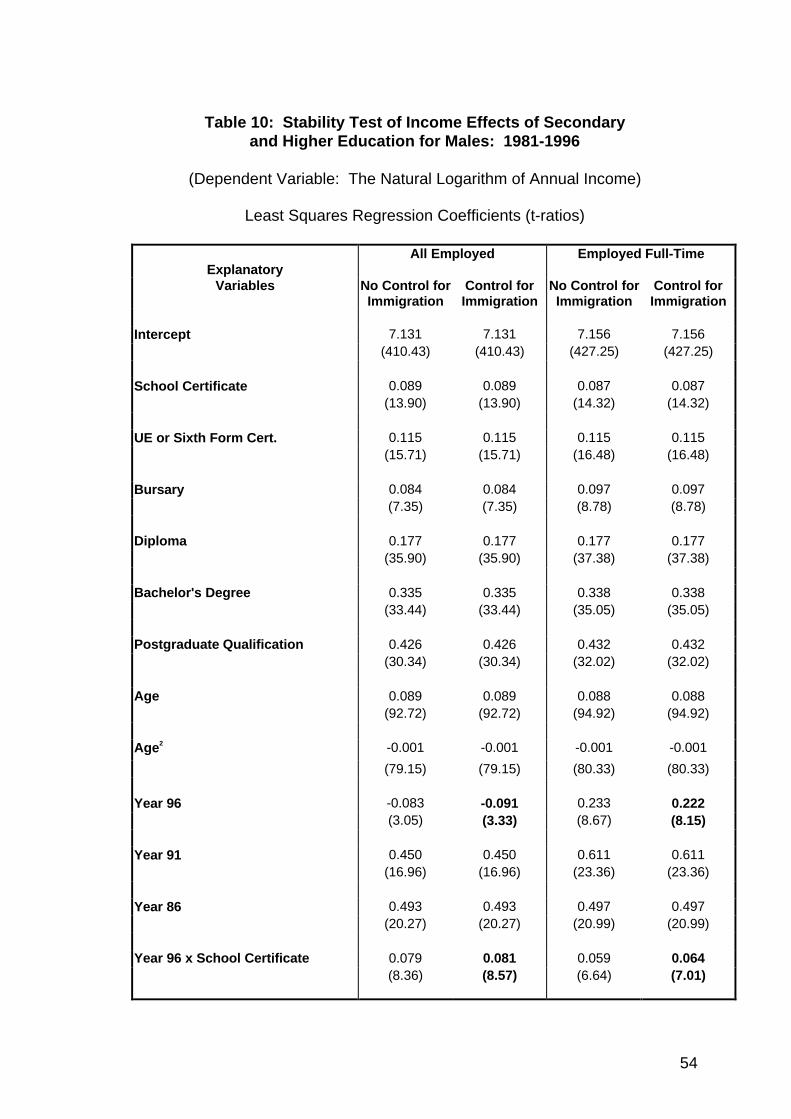
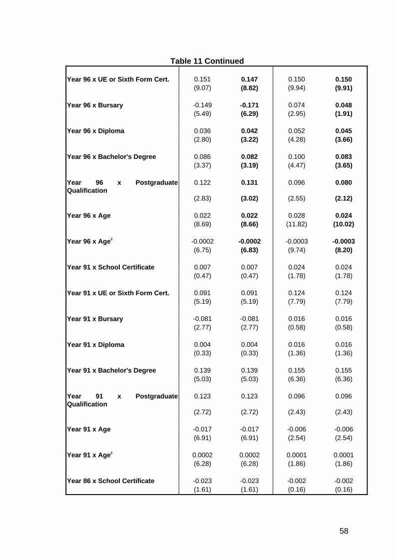
For the stability tests over the four census years, restricted and unrestricted models, the

binary variable technique and the Wald test are performed.19 The tests involve pooling

together the 10 per cent samples for the four census years. The stability of each

coefficient is tested through t-tests relating to interaction effects for all coefficients over

the four census years. The results of the non-restricted regressions for all employed and

19 For more details on the tests, the reader may refer to Ramanathan (1992), pp. 171-172,

and 274-276.

15

full-time employed males and females are summarised in columns 1-4 of Tables 10 and

11 respectively.

Figure 5 provides a summary of percentage income returns to various degree levels over

the four Census years, based on Tables 6-10. Figure 5 shows the increase in post-

compulsory secondary and tertiary income returns over the 15 year period, where the

solid lines represent the overall population and the broken line segment shows returns for

the 1996 population excluding recent immigrants since 1991. Also, implicit in these

results are the lower relative income levels with no school qualifications over the time

period, indicating that, in relative terms, the opportunity cost of not having school

qualifications has increased.20

As shown in Figure 5, the results in columns one and three of Tables 10 and 11 show that

the returns to all educational degrees were significantly higher in both 1996 and 1991

compared to the base year of 1981. These tests also indicate that the returns to most

educational qualifications had increased at statistically significant levels over the 1981-

1996 period. For example, the results for the sample of full-time employed males in

column three of Table 10 indicate that, compared to those without school qualifications,

the returns to School Certificate were 6.1 per cent higher in 1996 compared to 1981, the

returns to Sixth Form Certificate were 15.1 per cent higher, and the returns to Bursary

were 9.1 per cent higher. 21

The returns to a Diploma were 6.9 per cent higher, a Bachelor’s degree 20.3 per cent

higher, and the returns to a Postgraduate degree 20.0 per cent higher in 1996 than in

1981. The Wald test for the stability of all coefficients was also conducted based on the

restricted and unrestricted models spanning the four census years. The results further

20 Also implicit in Figure 5 is that while income returns to both secondary and tertiary qualifications

have increased over the four Census years, there has been a relatively greater rate of growth ofincome returns to Year 12 compared to tertiary education, as may be reflected by the marginalincome returns to tertiary education compared to Year 12 education.

.21 Respectively, with coefficients of 0.059, 0.141, and 0.087.

16

support the hypothesis, at the 0.01 level of significance, that overall the coefficients have

changed over the four census years, but most significantly between 1981 and 1991.22

A comparison of the results for males and females further confirms that the returns to

higher education have been higher for females since 1981. However, the relative

increases in the rates of return for females were more modest than they were for males

over the 1981-1996 period. Most significantly, in 1996 and compared to 1981 the returns

to a Bachelor’s degree for the sample of full-time employed females had increased by

10.5 per cent (a coefficient of 0.10 in 1996, in column three of Table 11), compared to an

increase of 20.3 per cent for males (a coefficient of 0.185). For a Postgraduate degree the

returns for females had increased by 10.0 per cent between 1981 and 1996, compared to

20.0 per cent higher for males.23

In addition, a comparison of the coefficients for 1996 and 1991 indicates that while for

males the returns to all educational degrees, including a Postgraduate degree, continued

to increase between 1991 and 1996, the returns to a Bachelor’s degree had decreased in

1996 relative to 1991. For example, for the sample of all employed males in column 1 of

Table 10 the coefficient reflecting the gain in returns to a Bachelor’s degree in 1996

relative to 1981 was 0.154 (indicating a percentage income increase relative to the control

group since 1981 of 16.6%) but the coefficient for the 1991 gain was 0.181 (indicating a

percentage income increase of 19.8% relative to the control group since 1981). For the

full-time employed sample of males the drop in the returns to a Bachelor’s degree

between 1991 and 1996 was more modest, as reflected by coefficients of 0.182 in 1996

and 0.197 in 1991. The results for females, in turn, indicate drops in returns to a

Bachelor’s degree in 1996 relative to 1991 and stable returns to a Postgraduate degree.

22 The reader may refer to Moulton (1986, 1991) in relation to using OLS estimation with grouped

data. Moulton shows that when individuals within a group are affected by a third omitted factorssuch as characteristics of a locality, or the state of the economy, the assumption that the errorterms across individuals, in different groups, are independent is no longer valid. Moulton’sanalysis shows that under these conditions the standard errors of the coefficients areunderestimated, and the statistical significance of the differences between groups will beoverstated. Two solutions are available. One is the introduction of dummy variables for eachcategory, such as the educational qualifications and Census year dummy variables included inthis study. When the introduction of dummy variables is not possible due to limited variationwithin groups (for estimation purposes) an adjustment in the standard errors or GLS arerecommended.

23 Respectively, with coefficients of 0.096 and 0.182.

17

It is of interest to examine the causes of the lower returns to a Bachelor’s degree in the

1996 compared to the 1991 census results. For example, as noted above, it is expected

that the returns to higher education would not increase indefinitely, and that when

demand for new skills increases educational institutions and students would respond to

the increased demand, such that the supply of graduates responds to demand. This

scenario, for example, is consistent with the finding that the returns to a Bachelor’s

degree have decreased slightly since 1991 for males, but that returns to a Postgraduate

degree have continued to increase, suggesting that the supply of Postgraduate degree

holders has continued to be smaller than demand.

However, it is important to note that the composition of the New Zealand population has

also been significantly affected through immigration since 1991. This is important to the

question of returns to higher education in 1996 relative to 1991, since changes in the New

Zealand immigration law and resulting immigration trends since 1991 have increased the

relative number of immigrants with higher education from non-English speaking

countries in the recent past. Fortunately, the 1996 census includes information on

whether or not those in the census were born overseas, and the year in which an

immigrant had migrated to New Zealand.24

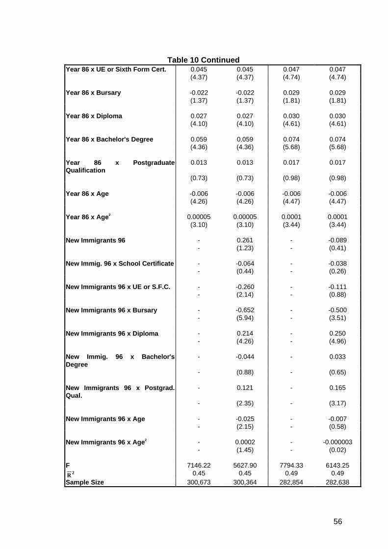
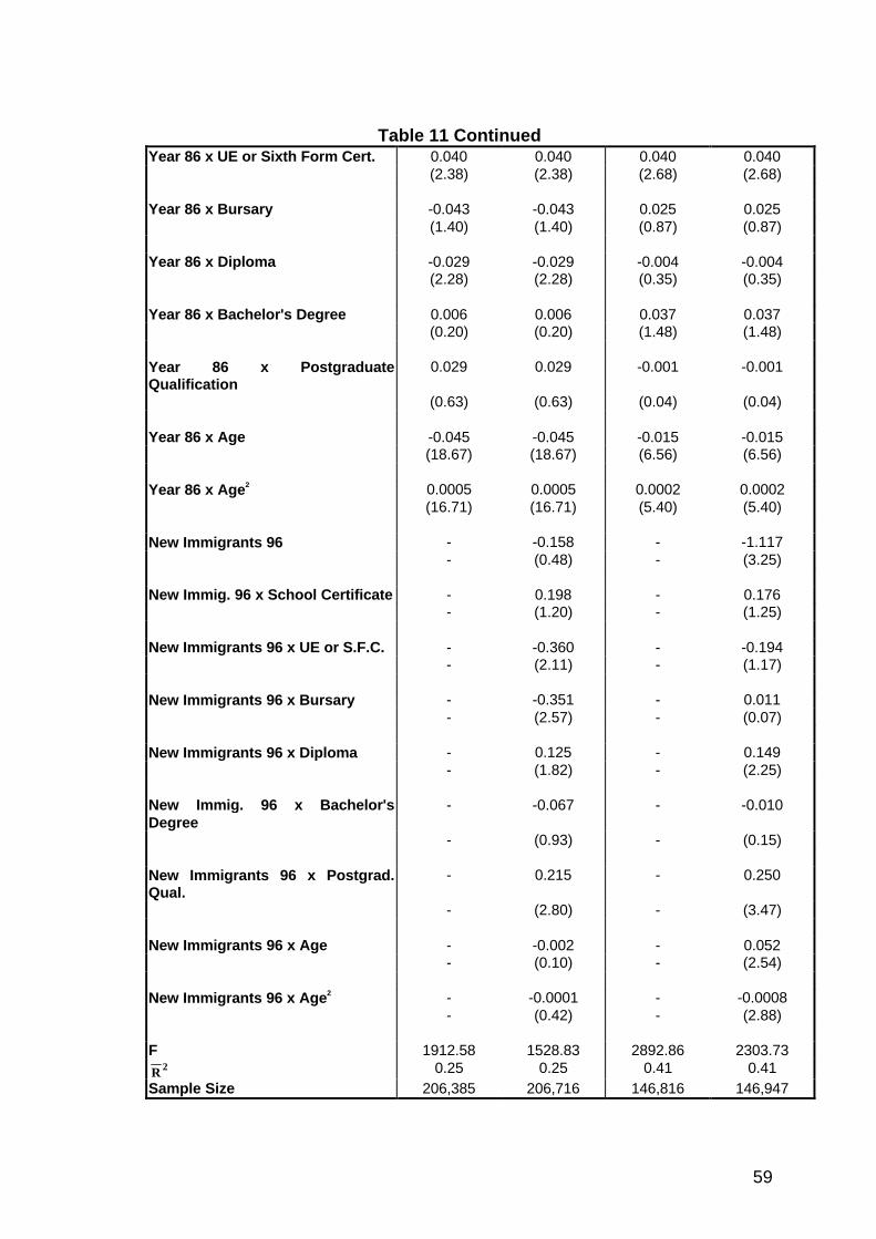
To adjust for the immigrant component of the 1996 census, since 1991, the models in

Tables 10 and 11 were expanded to adjust for returns to all educational degrees also

controlling for whether or not a respondent had immigrated since 1991. These results are

summarised in columns 2 and 4 of Tables 10 and 11 for males and females respectively.

These models allow the separate estimation of the returns to various educational degrees

in 1996 relative to the previous census years for the general population as opposed to

recent immigrants since 1991.

The results in columns 2 and 4 of Tables 10 and 11, also shown by the broken lines in

Figure 5, which control for the new immigrant population, show an important finding

24 The census also includes information on whether or not an immigrant had deficiencies inspeaking English.

18

that the results in columns 1 and 3, of a decline in the returns to a Bachelor’s degree in

1996 are actually reflecting the immigrant group results. This result is noteworthy, as

immigrants since 1991, who have by design of the immigration policy tended to have

higher education, and more significantly representative of non-English speaking

countries, are receiving lower returns to higher education, decreasing the average

estimated returns to Bachelor’s and Postgraduate degrees. The inclusion of the

immigrant population in the sample influences the estimates for the male sample to a

greater extent, but to a lesser degree for females. This is expected to reflect higher male

tertiary educational qualifications and labour force participation rates among certain

immigrant groups.

It can be noted in columns 2 and 4 that once the recent immigrant group is accounted for,

the results show that the male New Zealand population has received returns to a

Bachelor’s degree which have generally stabilised between 1991 and 1996. For example,

the coefficient of the income gain pertaining to a Bachelor’s degree in 1996, compared to

1981, in column 4 of Table 10 for full-time employed males changes to 0.202 compared

to 0.197 for 1991. Likewise, the gain in the returns to a Postgraduate degree in 1996,

compared to 1981, changes to 0.200 compared to 0.167 in 1991). This reverses the

results in columns 1 and 3 for males and it indicates that the demand for Post-graduate

degrees has continued to increase relative to the supply of graduates (when excluding

immigrants since 1991).

For females, in turn, the inclusion of the immigrant variable results in minor changes in

the coefficients, indicating that the returns to a Bachelor’s degree had decreased between

1991 and 1996, but that the returns to a Postgraduate degree also increased during that

time period. The results for a Bachelor’s degree reflect the relatively larger size of the

male immigrants with higher education in the labour force, and possibly other

characteristics of the samples of male and female immigrants in the labour force, such as

the country of origin of immigrants or language proficiency.

Although outside the scope of the current study, the labour market experience and the

relative earnings of recent immigrants are worthy of closer consideration in future

studies. For example, further tests of the returns to higher education based on the 1996

census for the immigrant population since 1991 (not presented here) confirm that the lack

19

of language proficiency is a significant factor which tends to decrease the returns to

higher education for this group. In addition, ‘years since migration’ are associated with

increased income and improved returns to a tertiary degree.

The analysis of this section has, however, shown that the returns to various education

levels have continued to be significant in 1996, and that between 1981 and 1996, and also

1986 and 1996 the returns have increased significantly.

IV. ‘Internal Rate of Return’ (IRR) Method

In this section private and social rates of return to post-compulsory education are

estimated using the Internal Rate of Return method, and comparisons are made to returns

based on the 1981, 1986 and the 1991 census years.

Estimates of private rates of return based on the IRR method estimate the discount rate

which equates the stream of lifetime gains from additional years of education to the total

personal costs of acquiring the additional education (see, for example, Psacharopoulos,

1981). The major strength of this method is that it can incorporate the effect of personal

costs of acquiring education such as student fees, and means of financing education plus

foregone earnings towards estimation of rates of return for various levels of education.

This is also true in the case of social rates of return, which incorporates public

expenditures on education.

Estimates of private rates of return to education generally incorporate the effect of

income gains in the form of lifetime after-tax incomes at a higher education level, in

relation to personal costs of education such as foregone earnings.

The IRR method assumes that the age-income profiles at a given time also reflect how an

individual may expect to earn income over his or her lifetime (see Psacharopoulos, 1981,

1985; Miller, 1982; and Behrman & Birdsall 1987). This rather restrictive assumption is

also implicit in the regression function method based on cross section data. The

alternative method of using longitudinal data sets has advantages for estimating ex-post

rates of return. However, for estimating ex-ante estimations a longitudinal data set has

20

the disadvantage of applying data over the previous half a century or so when the

economic conditions are likely to have been different as well. Therefore, the use of cross

section data, although not ideal, may best explain the returns expected by individuals

based on observable income gains at a given time.

The use of data from the four Census years has, however, allowed the creation of pseudo

panels of age income profiles as shown in Figures D1 to D4 in Appendix D. The panels

demonstrate the profiles for three age group cohorts followed through the four Census

years, such that the first cohort, for example, was 21-25 years old in 1981, 26-30 in 1986,

31-35 in 1991 and 36-40 in 1996. Age income profiles created on the basis of these

cohorts and the four Census years in real terms (with incomes in 1996 dollars) for

Bachelor’s degrees and Year 12, for males and females and 3 age cohorts are available in

the Appendix. It is interesting to note that these constructed age-income profiles follow

the shape of the portions of the cross-section profiles.25

Private Rates of Return

This method, which is referred to as the ‘elaborate method’ (see, for example,

Psacharopoulos, 1981, and 1994), involves in the first step deriving age-income profiles

through equations of the form:

Y a b ci i i= + +AGE AGE( )2 (2)

for each of the relevant education levels, and for the eight samples of males and females

in the categories of all employed, employed full-time, employed and unemployed, and

employed and out of the labour force.26

25 These age-income profiles use the 10% samples of the All Employed and before tax income

levels.26 It may be noted that equation (2) assumes a linear form as opposed to the semi-log

functional form of equation (1) (in relation to the dependent variable). The linearfunctional form is used in the IRR literature for the convenience of using estimatedincome levels in solving equations (3) and (4). The test of comparative semi-logfunctions, however, resulted in similar results for the rates of return based on the linearfunction at the mean.

21

In the second step, the estimated values of lifetime income (Y) are predicted for each

education level, and these predicted returns are used in solving equation (3) in deriving

the private rates of return to education (r):

[ ( ) ( )]

( )

[ ( ) ]

( )

Yh x Ys x

r

Ys x P

ri i t

tt S

ni i t

tt

S1 1

1

1

11 1

− − −

+=

− +

+= + =∑ ∑

(3)

where Yh and Ys respectively represent before-tax incomes with the higher and the lower

levels of education, and x is the income tax rate for the income level, such that after-tax

incomes are incorporated. Pi represents personal expenditures on education per year, t =

1 is the first time period of study for each degree, r is the discount rate, and S is the

number of years required for an educational qualification.27

In examining the private returns to education based on the 1996 census it is important to

note that to realistically reflect personal costs in estimating the net personal returns to

tertiary education, Pi in 1996 includes fees. For this, a weighted average of university

fees in New Zealand was estimated and included in the analyses. To provide results that

are updated and are most relevant, throughout this section the 1996 returns are based on

income levels and costs that are adjusted to 1998 dollars. The analysis also uses 1998

tertiary fees. The weighted average of university fees in New Zealand was estimated at

$2,877 in 1998. This weighted average was based on measures of the average fee

charged by each university in 1998 weighted by the number of each university’s

Equivalent Full-Time Student (EFTS) funded places for 1998. The details of the

calculation of the average fee are also presented in Appendix E.

In addition to the IRR estimations, discounted private sums of net returns for the relevant

degree are calculated by taking the net present value of all lifetime private income gains

discounted at a five per cent real discount rate minus the discounted sum of costs.

Expressed algebraically, this becomes:

27 A qualification enters the analysis once it is fully completed, and foregone earnings are

based on the most recently completed qualification.

22

N pvtYh x Ys x Ys x P

ii i t

tt S

ni i t

tt

S

( )[ ( ) ( )]

.

[ ( ) ]

.=

− − −−

− +

= + =∑ ∑1 1

105

1

1051 1 (4)

These sums are adjusted to 1998 dollars across the four census years for the convenience

in comparisons. It may be noted that in cases in which a private rate of return is less than

5 per cent, the corresponding sum of return which is discounted at the 5 per cent level

will be negative.

The private rates of return estimated for the census years of 1981, 1986 and 1991 and

1996 respectively use the marginal tax rates of the 1980-81, 1985-86 and 1990-91, and

1995-1996 tax years for calculating after-tax income.28 These estimates are based on

individual level data.29

In estimating lifetime earnings, it was assumed that, after completing their degree,

individuals work to the age of 65, and forgone earnings were estimated based on the

required number of years for completing a degree. It was assumed that a Bachelor’s

degree requires three years, a Postgraduate degree two years, and a Diploma two years

for completion. These are the general time requirements in New Zealand. Any

individuals taking longer than usual to complete a degree, or studying at advanced ages,

will face lower rates of return than those estimated in this study.

For example, to calculate the 1996 private rate of return for females with Postgraduate

qualifications compared to no secondary qualifications, there are eight years of foregone

earnings. Personal expenditures on education include tertiary fees in 1996, fees are not

included in the estimations for 1981 to 1991 census years since in those years tertiary

students were not subject to tuition fees, and student allowances also covered

28 Similar to the regression function method, the marginal tax schedules for a single person

without deductions have been used for calculations of after-tax income.

29 As noted earlier, the income information in the New Zealand census is reported in 13categories, based on annual gross income. The midpoint of these categories has beenused as a measure of income throughout the study. Age in the census is measured inactual years (rather than categories) and the analyses throughout the book incorporateactual years.

23

expenditures on text books. Therefore, the expected effect of tertiary fees is a decreasing

effect on the private rates of return for tertiary education in 1996, compared to 1991.

The left hand side of equation (3), or lifetime gains from education, are the higher yearly

net incomes (at 1996 tax rates) that a full-time female with a Postgraduate qualification

can earn on average above a full-time female with no secondary qualification, from the

time of completion of studies to age 65. The sum of benefits is set equal to the costs of

the foregone earnings to solve for the private rate of return (r).

The results for the private rates of return for all employed, and employed full-time, males

and females are presented in Table 12. Comparable private rate of return estimates over

the 1981-1996 census years are presented in Tables 13 and 14 for males and females

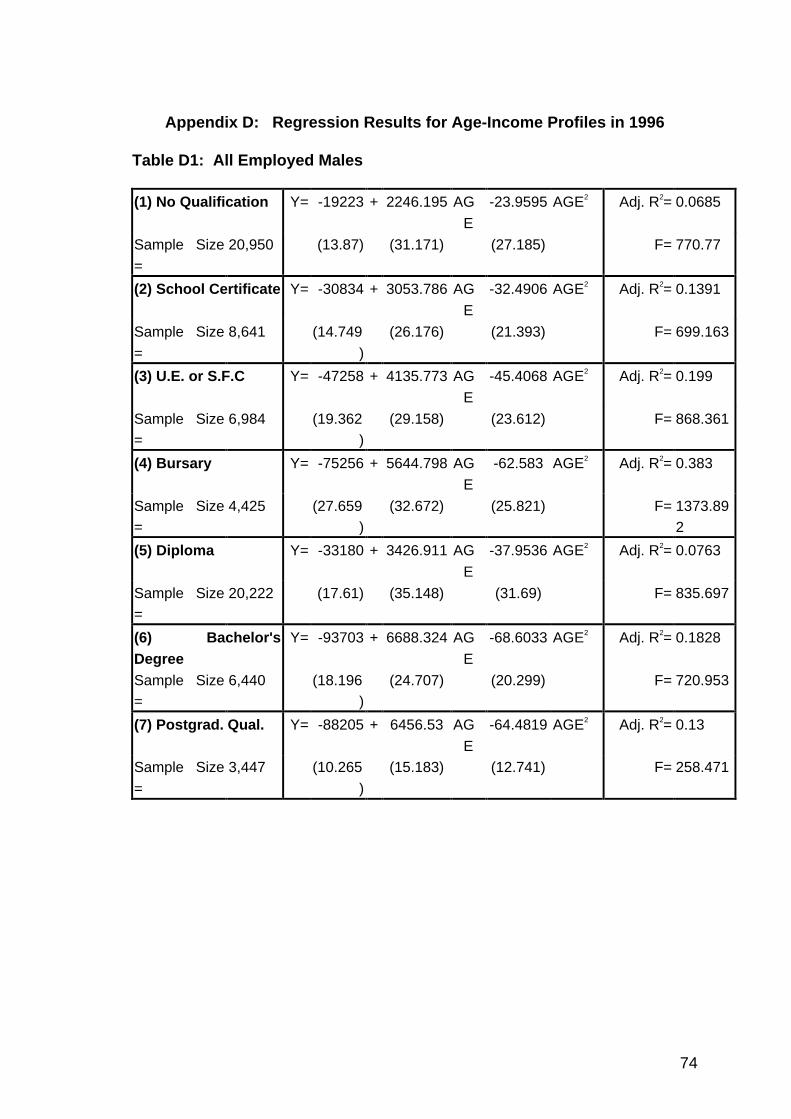
respectively. The results of age-income regressions for the seven education levels based

on equation (2) for 1996 are, in turn, presented in Tables D1 to D4 in Appendix D. These

equations provide average before-tax income levels for each education category by age

and gender based on the 1996 census. Since such results based on individual level data

and in a compatible form over time have not previously been available in New Zealand,

these results are provided to facilitate further research and analysis in this area.

Comparable results for the 1981-1991 census years may be found in Maani (1994 and

1997). The IRR method utilises the overall 1996 samples of New Zealand population

including immigrants since 1991, and therefore includes the combined effects of change

over time.

The results in Table 12 are compatible with the earnings function estimates in indicating

that education is a profitable investment for both males and females, although the

magnitude of these estimates is not identical to the earnings-function estimates. As

expected, the internal rates of return are lower than the regression function estimates, but

these differences are significantly larger for higher education levels with higher foregone

earnings.

For the sample of all employed, the rates of return from School Certificate to a Diploma,

in Table12, are 6.9 per cent for males and 3.6 per cent for females, and returns to a

Bachelor’s degree (in relation to Year 12 Sixth Form Certificate) are 9.2 per cent for

males and 9.8 per cent for females. These estimates, which incorporate foregone

24

earnings and tertiary fees are significantly lower than the regression function estimates.

This comparison has highlighted the need for caution in comparing rate of return

estimates from one method to the other, especially when foregone earnings are important

to the analysis.30

Similarly, the IRRs to males for a two-year Postgraduate degree in 1996 are around 5.1

per cent (compared to returns of 10.8 per cent with the earnings-function method, based

on a differential coefficient of 0.103 (or the difference: 0.598 - 0.495) from column one

of Table 4)). As before, for a Postgraduate degree, the estimated returns for females were

higher at rates of 8.00 per cent using the ‘elaborate method’ (but lower than the estimates

of 17.8 per cent with the earnings-function method, based on a differential coefficient of

0.164 (or the difference: 0.679 - 0.515) from column one of Table 5).

Like the regression function results for the 1981, 1986 and 1991 census years, the returns

to School Certificate and Sixth Form Certificate are significant and above ten per cent,

but the rates of return for each additional year of education beyond the Sixth Form are

lower than ten per cent.31

The rates of return and the sums of return in Tables 13 and 14 further allow comparisons

of private rates of return with the IRR method over the four census years. These results

show that the returns for most educational degrees have increased throughout the 1981 -

1996 period, and that only in the case of a Bachelor’s degree have the rates of return

decreased, by generally less that one percentage point. This result is expected to reflect

the effect of fees, increases in returns to year 12 studies over the period, changes in the

supply of graduates, and the immigrant composition of the population.

30 When the returns to a Bachelor’s degree compared to the sample with Bursary are

considered, returns to tertiary education are estimated at higher rates. As noted earlier,this is due to the somewhat lower levels of income for the Bursary sample both as thebase for comparison and for foregone earnings. There is also one less year of foregoneearnings.

31 The rates of return for Sixth Form Certificate to Bursary, and to Diploma, are oftennegligible, negative or undefined. Undefined rates of return occur where all lifetimeincome differentials at the higher education level are adverse (and consequentlycalculation of a rate of return is not possible), or where most of the lifetime incomedifferentials are adverse.

25

Social Rates of Return

The analysis of the social rates of return to education examines the rate of return

associated with lifetime income gains adjusted for all public and private costs of this

investment including foregone earnings. The use of lifetime income gains from

education is based on one of the underpinnings of micro-economic theory: that in

competitive markets the market returns to one’s economic activity (or earnings) reflect

the value the economy places on one’s productivity. Therefore, if on average, income

earned due to employment or other market activity reflects the value of one’s market

productivity, the effect of education on increased productivity should be captured through

income gains.

The calculation of the social rates of return ( rs ) is in turn based on equation (5) below,

incorporating foregone earnings, Ysi and personal expenditures, Pi, as well as

government expenditures, Gi, on education at time t:

[ ]

( )

[ ]

( )

Yh Ys

r

Ys P G

ri i t

st

t S

ni i i t

st

t

S−

+=

+ +

+= + =∑ ∑

1 11 1(5)

where Yh and Ys respectively represent before-tax incomes with the higher and the lower

levels of education, in correspondence to their theoretical counterpart of market rewards

as a reflection of the value the economy places on the productivity of labour with that

qualification level. (The private rates of return in comparison incorporated after-tax

incomes in correspondence to the returns accruing to the individual).

Government expenditure levels used in the analysis for 1996 are based on the most recent

estimates of annual costs of secondary and tertiary education as provided by the Ministry

of Education for three levels: Secondary School, Polytechnic and University level. The

estimated total annual government expenditures in 1994 per student per year were

reported as follows: $5,030 for the secondary school level, $9,210 for polytechnics, and

$10,170 for the university level. These per-student expenditures include operating grants,

salary costs and external costs including central administration expenditures and support

services such as the administration of the student allowance scheme. (In 1990, the per

26

student expenditures for a university degree were higher at $11,658).32 Finally, as before,

Pi represents personal expenditures on education per year (which again was assumed to

be zero in the 1981 - 1991 census analyses, but it takes the estimated value of $2,877 for

the average weighted value of tertiary fees in the 1996 census analysis), t = 1 is the first

time period of study for the relevant degree, rs is the discount rate, and S is the number of

years required for an educational qualification.33 Therefore, in comparisons of the 1996

social rates of return to education compared to the earlier census years, the overall

expenditures on education includes both the government spending, student fee payments

and foregone earnings.

Correspondingly, the net social discounted sums of returns may be expressed

algebraically as:

N socYh Ys Ys P G

ii i t

tt S

ni i i t

tt

S

( )[ ]

.

[ ]

.=

−−

+ +

= + =∑ ∑

105 1051 1 (6)

multiplied by the price level conversion factor. As before, any social rate of return of less

than five per cent will have an associated negative sum of return at a five percent

discount rate.

It may be noted that, ideally, social rates of return to education must incorporate the

externalities of education to include not only returns to education in the form of earnings,

32 (Source: Education Statistics of New Zealand 1998). The estimated total annual

government expenditures in 1990 per student per year were in turn reported as follows:$4,596 for the secondary school level, $9,605 for polytechnics, and $11,658 for theuniversity level (Source: Horan, R. and N. Pole (1993), Government Expenditure onEducation: 1990, Report by the New Zealand Ministry of Education, Table 6, p. 18).These expenses were adjusted for inflation in estimates of the 1981 - 1991 social rates ofreturn to education. If capital valuation of educational institutions was added to the costs,they became $5,367, $12,583 and $14,891 respectively. The breakdown of the $14,891annual expenditures per student at the university was $3,513 in salary costs as part of$8,697 of operations grant, in addition to $2,961 of external costs (for example, schooltransport and student allowances), and $3,233 for capital valuations. The reader mayalso consult Marais (1992) and Hope and Miller (1988) for further discussions of financingtertiary education.

33 An educational qualification enters the analysis once it is fully completed, and foregoneearnings are based on the most recently completed qualification. Degree costs reportedin 1990 in real terms were used for the three census years.

27

but the net pecuniary and non-pecuniary benefits to third parties in an economy. A wide

range of benefits associated with education has been identified in the literature.

Examples of the spill-over benefits cited include a greater ability to take initiative,

develop and adapt to technological change in the workplace (Chapman and Chia, 1989);

improved health; a role in preserving democratic freedom, in transmitting cultural values

(McMahon, 1987); a role in more intelligent voting behaviour (Brennan, 1988); and a

role in lowering criminal behaviour (Webb, 1977). The negative association between

educational qualifications and unemployment has been addressed in detail for New

Zealand, in the OECD Economic Surveys 1992-1993.34 There is also evidence that those

with higher education are less likely to depend on welfare payments (Chia, 1990; Maani,

1994).

Considering such external benefits is obviously relevant to the decision-making process

regarding the funding of education. However, the international literature on social rates

of return has come to exclude such external benefits, since identifying and measuring

these benefits objectively is extremely difficult. As a result, what is referred to as the

‘social rates of return’ to education in the literature and in this study is not fully

equivalent to its theoretical counterpart, since the empirical measure includes the public

expenditures on education but not third party benefits such as the advantages of a well

trained labour force. In the analysis of this section, the conventional method of

estimating social rates of return has been adopted, with zero values assigned to the

external benefits of education. Therefore, as with the earlier census estimates, the

estimated values are best interpreted as minimum social rates of return.

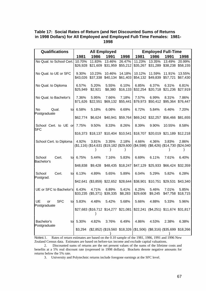
The estimates of the social rates of return to education, for males and females, are

presented in Table 15, and comparable returns for 1981-1996 for males and females are

presented in Tables 16 and 17. The results indicate that investment in education

continues to be socially profitable in 1996 as was estimated for the three previous census

34 A number of monetary and non-monetary externalities of tertiary education are also noted

in the New Zealand Vice-Chancellors’ Committee Report (1993).

28

years, and similar to the private rates of return, at rates which diminish for higher levels

of education (per year of study).35

An examination of the results for 1996 in Table 15 and over time in Tables 16 and 17

indicates that the social rates of return have been positive and have generally either

increased or remained relatively stable over the decade. The social rates of return for all

employed, and full-time males in 1996 for completing the Sixth Form Certificate

compared to No School Qualifications (in columns one and three of Table 15), are 13.3 to

12.9 per cent, and 14.2 to 13.5 per cent for females. These social rates of return indicate

that investment in education is not only privately but also socially desirable, compared to

a wide range of investments with lower rates of return. These rates of return are about

1.9 -2.2 per cent lower than the private rates of return for males, and 2.7-3.6 per cent

lower for females. 36

The social rates of return to a Bachelor’s degree, from Year 12 are 8.1 - 8.6 per cent for

males, and 7.4 to 7.8 per cent for females. These social rates of return are respectively

around 2.4 to 2.6 per cent lower than the private rates of return for males and around 1

percentage point lower than the private rates of return for females. The social returns to a

Postgraduate degree have also increased in 1996 for both males and females (at

estimated returns of 4.16 to 4.59 per cent), compared to higher returns of 6.38 to 6.49 per

cent for females. The relative rates of return to a Bachelor’s and a Postgraduate degree

again reflect the effect of higher foregone earnings once a Bachelor’s degree is obtained.

However, consistent with the results for the earlier census years, the 1996 age-income

profiles as shown in Figures 1–4 based on annual incomes, and the earnings function

method in Tables 5-10 have shown that the market income levels do reward a

35 Considering capital valuations as a part of costs of education is relatively recent in New

Zealand and was used in the early 1990s. Incorporating capital valuations in IRRestimations has been examined in detail in Maani (1994) for comparative purposes. Thisdecreases the social rates of return by less than one per cent.

36 Similar to the private rates of return, beyond Sixth Form Certificate, the social rates of return foreach additional year of education are lower than ten per cent. The social returns to a Diploma,compared with School Certificate and excluding a seventh form year, are about two per centlower than the private rates of return for males at 4.4 per cent (compared to 6.93 per cent), andabout one and a half per cent lower than the private rates of return for females at 2.18 per cent(and 3.62 per cent).

29

Postgraduate degree above a Bachelor’s degree, as reflected by higher average income

levels.

Vaillancourt (1986), who has used similar methods for estimating private and social rates

of return to a Bachelor’s degree for Canada in 1981, estimates returns of ten per cent for

private and six per cent for social rates of return in British Colombia. Private rates of

return in other regions are estimated at nine to fourteen per cent, and social rates of return

at seven to nine per cent. Miller (1982) had found private returns of twenty-one per cent

and social returns of fifteen to sixteen per cent for a Bachelor’s degree based on the 1976

Australian census. Private rates of return for Postgraduate degrees were estimated at 14.5

to 14.8 per cent and social rates of return at 10.1 to 10.7 per cent (based on the 1976

Australian census).

In a recent summary of international estimates of private and social rates of return

(Psacharopoulos, 1994), the overall private rate of return to secondary education was 17.7

per cent and for higher education 19.0 per cent, compared to social rates of return of 13.5

per cent and 10.7 per cent respectively. In these estimates, the differences between the

private and social rates of return (differences of 4.2 per cent for secondary education) are

significantly greater than the estimates of this study.

In the 1981-1996 results for New Zealand, the differences in the private and social rates

of return to education are, in general, consistently modest at differences of one to four per

cent for the three census years. In these differences New Zealand continues to be closer

to the group of high income countries (reported in Psacharopoulos (1994) with private

rates of return of 12.8 per cent to secondary education and 7.7 per cent to tertiary

education, and social rates of 10.3 per cent and 8.2 per cent respectively), than it is to the

rest of the world, due to the well-established income tax system in New Zealand and

other higher income countries.37

Since virtually all countries subsidise education to some extent, the social rates of return

to education ( rs ) calculated as above are often lower than the private rates of return (r).

In these measures, since the private rates of return are based on after-tax income, and

37 High income countries are specified at income levels of $7,600 and higher in that study.

30

social rates of return are based on before-tax income while incorporating public

expenditures on education, the differences between the two rates are expected to be

affected by the income tax system relative to public expenditures on education.

However, it may be noted that the difference between the private and social rates of

return to education is only a crude measure of government subsidisation of education,

since government expenditures and income tax payments are practically discounted at

different discount rates in the private and social rate of return estimations.38

Two alternative comparisons to the above differences are also possible. One is to

examine the difference between the net sum of the social and private present values for

each educational degree. This difference is derived by subtracting equation 4 from

equation 6 [ N soc i( ) - N pvt i( ) ], where these equations use a standardised discount rate and

are expressed in dollar terms.39 These differences may be derived from the sums of

return for each education level in columns 1 and 3 of Tables 15 and 12 for males, and

columns 2 and 4 of the same tables for females. These differences are in dollar terms,

and they are discounted at a uniform rate of 5 per cent, reported in 1998 dollars for

comparison across the years.

These differences are generally positive, indicating that, assuming a forty year working

lifetime, additional potential income tax payments are estimated at levels generally

greater than the average government subsidy of education.

In interpreting estimates of social rates of return to education it should be recognised that

these estimated rates of return are significant, even though a value of zero is assigned to

positive externalities of education. Therefore, the estimates in Tables 15-17 may be

interpreted as minimum estimates for expected social rates of return.

38 This may be verified algebraically by subtracting equation 3 from equation 5 with differentvalues for the discounting rate for the private and social rates of return .

39 The reader may verify algebraically that the difference is equivalent to:

[ ( ) ( )]

( . )

[ ]

( . )

[ ( )]

( . )

Yh x Ys x

t S

nG

t

SYs x

t

Si i t

ti t

ti t

t

−

= + = =∑ ∑ ∑− −

1 051

1 051

1 051

or the net present value of the sum of additional income taxes over a working lifetime,minus the present value of government expenditures for the degree and foregone incometaxes during the years of education, all discounted at a uniform rate.

31

Finally, an implication of these results is that individuals and secondary and tertiary

teaching institutions are together providing economic value that is reflected by greater

access to employment and higher productivity, the value of which may be estimated

through market valuations reflected by higher lifetime incomes.

V. Conclusion

This study has provided updated measures of private and social rates of return to

education for New Zealand, using unit record data from the 1996 census. The two

methods of regression analysis and the Internal Rates of Return (IRR) were employed,

and the analysis provided comparable results for both the private and social rates of

return to secondary and higher education over the four census years of 1981, 1986, 1991

and 1996. In addition, formal stability tests were conducted, based on the regression

method, to examine the potential change in the rates of return between the 1981 and each

of the later census years.

A number of results in 1996 are compatible with the results for the earlier census years.

However, some unique features of the 1996 results are also significant.

The 1996 results are consistent with the earlier results in confirming that the returns to

both secondary and tertiary education are significant and that compared to 1981, returns

to all educational qualification levels were significantly higher in 1996. Similar to earlier

findings, age-income profiles were flatter for females than for males in 1996, and the

private rates of return to education with the ‘earnings function’ method were higher than

the estimates with the IRR method which directly incorporate foregone earnings and

other costs of education, especially at the tertiary level due to higher foregone earnings.

The private rates of return for females were also higher than for males for various

education levels, despite the lower average income levels of females, reflecting an

income gain for females with higher education levels compared to other females with less

education who are engaged in jobs which pay less.

32

The results based on the IRR method show that both the private and social rates of return

to the various educational degrees have continued to increase throughout the 1991-1996

period. An exception is the private rates of return to a Bachelor’s degree, compared to

UE or Sixth Form Certificate between 1991 and 1996, which has decreased by less than 1

percentage point for males, and by less than 2 percentage points for females.40 This

result is consistent with the regression analyses shown in Figure 5. As discussed earlier,

this decline reflects the effect of tertiary fees, changes in the supply of graduates and the

immigrant composition of the population since 1991.

The social rates of return to all education levels have generally increased between 1991

and 1996, including the returns to a Bachelor’s degree. Among the factors contributing

to this result are that the government costs of financing a tertiary degree have decreased

since 1991, and the introduction of student fees, which affects the private returns to

education, does not change the overall cost of education faced by the society.

A result that is prominent in the IRR analyses for both males and females is that the

private and social returns to Postgraduate degrees have increased between 1991 and 1996.

This is consistent with the hypothesis that the supply of Graduates with Bachelor’s

degrees has been more elastic than the supply of Postgraduates in meeting the market

demand due to the time requirements of the Postgraduate degree. In addition, the

increased demand for university graduates and the increased returns to a Bachelor’s

degree, as reflected by the 1991 Census, have resulted in higher foregone earnings in

pursuing Postgraduate studies resulting in a relatively less elastic supply of Postgraduate

degree holders, and a greater rise in the Postgraduate labour market income premium by

1996.

The results based on the regression method (which excludes the effect of tertiary fees) are

compatible with the IRR results. A result that is consistent throughout the analyses is that the

returns to both secondary and tertiary qualifications have increased significantly during the

40 For males the return to a Bachelor’s degree, compared to the control group,

changed from 10.1 - 10.4 % in 1991 to 9.2 - 9.8 % in 1996, in columns 3-4 and 7-8 of Table 13. The comparable decrease for females is from 9.1 - 9.4 % in 1991to 7.1 - 7.3 %, in columns 3-4 and 7-8 of Table 14.

33

1981- 1996 and the 1986-1996 periods. For example, the stability test results for 1996 and

comparisons to 1981 indicate that the returns to a Bachelor's degree had increased by 22.3%

over the 15 year period for the sample of full-time employed males, and they were 8.6%

higher for females.41 The returns to a Postgraduate degree were also 22.1% higher for full-

time employed males in 1996 and 8.3% higher for females.

In addition, the regression results show consistent evidence on increases in returns to

most educational degrees for both males and females between 1981 - 1996, and between

1981 and 1991, but diverging results for males and females since 1991 as reflected by the

1996 regression analyses.

The returns to a Bachelor’s degree, in particular, represent declines between 1991 and

1996 for females and a stabilisation of market income premiums for males. A plausible

explanation for this is, of course, the increase in the supply of graduates in response to

demand, between 1991 and 1996, in fields of study where there have previously been

shortages. These results further suggests that some of the features of the market and the

earnings for males and females in 1996 may have been different from the earlier years,

such as the composition of the population. This indicates that a more in depth analysis of

the 1996 census for males and females over a wider range of variables would be useful.

For example, one of the notable features of the New Zealand population in 1996 is a

greater significance of immigrant numbers with higher education since 1991. To adjust

for the population’s immigrant composition, such that a comparable population was

considered in 1991 and 1996, extensions of the stability tests adjusted for immigrant

status since 1991. These results highlight the significance of adjusting for the immigrant

composition of the population for comparisons of market returns to tertiary education

prior to and after 1991. Most significantly, the results indicated that for comparable

populations over time, the market returns to a Bachelor’s degree have been generally

stable between 1991 and 1996 (e.g. showing a small increase of 0.005 %) for full-time

employed males, and an increase of 3.3%, for a Postgraduate degree.

41 These comparisons are based on the regression method for the sample of the full-time

employed and compared to the base group with qualifications below a School Certificate.

34

The results for the sample of full-time employed females, in turn, continued to show a

decline in the returns to a Bachelor’s degree of 7.2% between 1991 and 1996, and a

decrease in the returns to a Postgraduate degree of 1.6% over the same time period. Of

course, the income gains to tertiary education may not be expected to increase

indefinitely, especially with supply adjustments, and the 1996 evidence indicates that a

stabilisation of the market for graduates has been in effect in the 1991-1996 period.

References

Anderson, L.1988 "Rates of Return of Education for Females in El Salvador." Social and EconomicStudies, 37, No. 3, 279-87.

Behrman, J.R. and N. Birdsall1987 "Comment on Returns to Education: A Further International Update andImplications." The Journal of Human Resources, 22, No. 4, 603-606.

Bossiere, M., J.B. Knight and R.H. Sabot1985 "Earnings, Schooling, Ability, and Cognitive Skills." American Economic Review,75, 1016-30.

Brennan, G1988 "The Structure of Tertiary Fees", Economic Analysis and Policy, 18, 171-185.

Chapman, B.J. and T.T. Chia1993 ;Income Contingent Charges to Higher Education: Theory, policy and Data from theUnique Australain Experment’, paper presented to the World Bank InternationalSymposium on the Economics of Education, May 1993, Manchester, U.K.

Chia, T.T.1990 Returns to Higher Education in Australia, PhD thesis, Australian national University.

Demetriades, E.L. and G. Psacharopoulos1987 "Educational Expansion and the Returns to Education: Evidence fromCyprus."International Labour Review, 126, No. 5, 597-602.

Dougherty, C.R.S. and E. Jimenez1991 "The Specification of Earnings Functions: Tests and Implications." Economics ofEducation Review, 10, No. 2, 85-98.

Evans, L, et. al.1996 “Economic Reform in New Zealand 1984-95: The Pursuit of Efficiency.” Journal ofEconomic Literature, 34 (4), 1856-902.

Grilliches, Z. and W. Mason1972 "Education, Income and Ability." Journal of Political Economy, 80, S 74- S 104.

Halvorsen, R. and Palmquist, R1980 “Variables in Semilogarithmic Equations” American Economic Review, 70, 474-75.

Heckman, J. and S. Polachek1974 "Empirical Evidence on the Functional Form of the Earnings SchoolingRelationship." Journal of American Statistical Association, 69, 350-354.

Heckman, J. et. al.1996 “Human Capital Pricing Equations With an Application to Estimating the Effect ofSchooling Quality on Earnings”, Review of Economics and Statistics, 78(4), 562-610.

36

Hope, J. and P.W. Miller1988 "Financing Tertiary Education: An Examination of the Issues." The AustralianEconomic Review, No. 4, 37-57.

Horan, R. and N. Pole1993 Government Expenditure on Education: 1990: Report by the New Zealand Ministryof Education.

Hunt, D. and J. Hicks1985 "Economic Returns to University Education in New Zealand." New Zealand Journalof Educational Studies, 20, No. 2, 170-85.

Jamison, D.T. and J. van der Gaag1987 "Education and Earnings in the People's Republic of China." Economics of EducationReview, 6, No. 2, 161-6.

Maani, S. A.1994 "Rates of Return to Higher Education in New Zealand: a Study of the Census Years1981-1991", Report prepared for the New Zealand Treasury, Wellington.

Maani, S. A.1996a"A Research Agenda, Methodologies, Models and Data Requirements For EstimatingParticipation in Post-Compulsory Education in New Zealand, Report prepared for the NewZealand Treasury, Wellington.

Maani, S A.1996b"Private and Social Rates of Return to Secondary and Higher Education in NewZealand: Evidence from the 1991 Census", Australian Economic Review, 113, 82-100.

Maani, S. A.1997 Investing in Minds: The Economics of Higher Education in New Zealand, Instituteof Policy Studies, Wellington.

Marais, T.1992 The Funding of Tertiary Education in New Zealand, University of Western AustraliaDiscussion Paper 92.26.

Mc Mahon, W.W.1987 "Externalities in Education", in G Psacharopoulos (ed.), Economics of Education:Research and Studies, Oxford, pergamon Press, 133-137.

McNabb, R. and S. Richardson1989 "Earnings, Education and Experience: Is Australia Different?" Australian EconomicPapers, 28, 57-75.

Miller, P.W.1982 "The Rate of Return to Education: Evidence from the 1976 Census." The AustralianEconomic Review, No. 3, 23-32.

Miller, P.W.1984 “Education and the Distribution of Earnings” in Blandy R. Covick, O. eds.Understanding Labour Markets in Australia, Allen and Unwin.

37

Ministry of Education1988 Education Statistics of New Zealand 1998. Government printing office, Wellington.

Moulton, B. R.1986 ‘Random Group Effects and the Precision of Regression Estimates’, Journal of

Econometrics, 32, 385-397.

Moulton, B. R.1990 ‘An illustration of a pitfall in Estimating the Effects of Aggregate Variable on MicroUnits’, Review of Economics and Statistics, 72(2) 334-338.

New Zealand Vice-Chancellors' Committee1993 OECD Economic Surveys 1992-1993 New Zealand: Human Capital Developmentand Economic Performance, A Critique. Occasional Paper No. 1.

O'Dea, D.1987 The Returns to Education in New Zealand, Unpublished Paper.

Olgilvy, B.J.1970 "A Cost Benefit Study of Education in New Zealand." New Zealand Journal ofEducational Studies, 5, No. 1, 33-46.

Psacharopoulos, G.1981 "Returns to Education: An Updated International Comparison." ComparativeEducation, 17, No. 3, 321-41.

38

Psacharopoulos, G.1985 "Returns to Education: A Further International Update and Implications." TheJournal of Human Resources, 20, No. 4, 583-97.

Psacharopoulos, G.1994 Returns to Investment in Education: A Global Update, World Development, 22 (9),1325-1343.

Ramanathan, R.1992 Introductory Econometrics with Applications, 2nd ed., Harcourt Brace JovanovichCollege Publishers.

Raymond, R. and M. Sesnowitz1983 "The Rate of Return to Mexican Americans and Anglos on an Investment in aCollege Education." Economic Enquiry, 21, No. 3, 400-11.

Rumberger, R.W.1987 "The Impact of Surplus Schooling on Productivity and Earnings." Journal of HumanResources, 22 (1), 24-50.

Ryoo, J-K.1988 "Changes in Rates of Return to Education Over Time: The Case Study of Korea."PhD Dissertation, Stanford University.

Schultz, T.P.1988 "Education Investment and Returns." In Handbook of Development Economics, ed.H. Chenery and T.N. Srinivasan. Vol. 1. North-Holland.

Silverstone, B., A. Bollard, R. Lattimore, eds.1996 A study of Economic Reform: The Case of New Zealand, Amsterdam, north Holland.

Tan, J-P and V. Paqueo1989 "The Economic Returns to Education in the Philippines." International Journal ofEducational Development, 9, No. 3, 243-50.

Vaillancourt, F.1986 "The Returns to University Schooling in Canada." Canadian Public Policy - Analysede Politiques, 12, No. 3, 449-58

Web, L.D.1977 "Savings to Society by Investing in Adult Education", in Economic and SocialPerspectives on Adult illitracy, State Department of Education, Tallahassee, Florida, 52-73.

Wilson, R.A.1985 "A Longer Perspective on Rates of Return." Scottish Journal of Political Economy,32, No. 2, 191-8.

39

Table 1: Characteristics of the Samples

Means(Standard Deviations)

Personal 1981 1986 1991 1996Characteristics Males Females Males Females Males Females Males Females

Age 37.18 37.46 37.19 37.45 37.13 37.03 38.33 38.27(13.92) (14.04) (13.65) (13.73) (13.34) (13.20) (12.86) (12.71)

Ethnic Origin(Percentage of Sample) European 84.52% 84.16% 84.59% 84.95% 78.26% 77.08% 79.25% 78.61% Maori 10.33% 10.60% 9.99% 9.83% 11.44% 12.30% 12.68% 13.29% Other 5.15% 5.24% 5.42% 5.22% 10.30% 10.62% 8.07% 8.10%

Income Current Dollars 12764.72 5277.36 18670.45 9718.79 25096.17 15072.55 31643.78 18235.17

(8866.46) (5161.39) (11180.80) (7618.66) (18018.10) (12152.60) (26433.75) (16876.39) 1996 Dollars 36280.47 14999.56 30674.94 15967.66 27502.30 16517.65 31643.78 18235.17

(25200.66) (14669.94) (18369.69) (12517.21) (19745.61) (13317.75) (26433.75) (16876.39)

Highest Qualification (Percentage of Sample) No Qualifications 50.08% 54.37% 36.04% 41.41% 33.41% 36.42% 34.06% 34.62% School Certificate 11.68% 14.71% 12.26% 17.17% 11.17% 15.83% 11.40% 15.59% U.E./Sixth Form Cert. 8.39% 9.00% 8.02% 9.42% 7.18% 8.68% 8.99% 11.04% Bursary 2.96% 2.26% 3.95% 3.13% 5.05% 4.40% 7.22% 6.34% Diploma 21.34% 16.92% 32.19% 24.25% 35.50% 29.47% 25.78% 22.40% Bachelor's Degree 3.72% 2.11% 4.64% 2.96% 5.11% 3.60% 8.17% 6.87% Postgraduate Qual. 1.83% 0.63% 2.90% 1.66% 2.58% 1.60% 4.38% 3.14%

Labour Force Status (Percentage of Sample) All Employed 88.83% 45.99% 87.07% 62.83% 74.46% 56.36% 80.41% 64.34% Employed Full-Time 85.91% 37.51% 81.31% 43.74% 69.66% 38.82% 73.62% 43.70% Unemployed 3.78% 2.72% 3.19% 4.35% 8.29% 6.64% 5.25% 4.89% Out of Labour Force 7.39% 51.29% 9.74% 32.82% 17.25% 37.00% 14.34% 30.05%

Sample Size 89505 88268 96741 90237 96140 96690 90854 93779

40

Figure 1: Age-Income Profile by Education Level forAll Employed Males in 1996 (Income in 1996 Dollars)

All Employed Males 1996

0.0

10000.0

20000.0

30000.0

40000.0

50000.0

60000.0

70000.0

80000.0

16-20 21-25 26-30 31-35 36-40 41-45 46-50 51-55 56-60 61-65

Age Interval (years)

Postgraduate

Bachelor's

Diploma

Bursary

U.E. or S.F.C.

School Cert

No Qual.

41

Figure 2: Age-Income Profile by Education Level forEmployed Full-Time Males in 1996 (Income in 1996 Dollars)

Employed Full-Time Males 1996

0.0

10000.0

20000.0

30000.0

40000.0

50000.0

60000.0

70000.0

80000.0

16-20 21-25 26-30 31-35 36-40 41-45 46-50 51-55 56-60 61-65

Age Interval (years)

Postgraduate

Bachelor's

Diploma

Bursary

U.E. or S.F.C.

School Cert

No Qual.

42

Figure 3: Age-Income Profile by Education Level forAll Employed Females in 1996 (Income in 1996 Dollars)

All Employed Females 1996

0.0

10000.0

20000.0

30000.0

40000.0

50000.0

60000.0

70000.0

80000.0

16-20 21-25 26-30 31-35 36-40 41-45 46-50 51-55 56-60 61-65

Age Interval (years)

Postgraduate

Bachelor's

Diploma

Bursary

U.E. or S.F.C.

School Cert

No Qual.

43

Figure 4: Age-Income Profile by Education Level forEmployed Full-Time Females in 1996 (Income in 1996 Dollars)

Employed Full-Time Females 1996

0.0

10000.0

20000.0

30000.0

40000.0

50000.0

60000.0

70000.0

80000.0

16-20 21-25 26-30 31-35 36-40 41-45 46-50 51-55 56-60 61-65

Age Interval (years)

Postgraduate

Bachelor's

Diploma

Bursary

U.E. or S.F.C.

School Cert

No Qual.

44

Table 2: Labour Force Status and Income of Males in 1996by Highest Educational Qualification

PersonalCharacteristics

No Qual. SchoolCert.

UE orSFC

Bursary Diploma Bachelor's Qual.

Postgrad.Qual.

Age 41.60 36.21 33.14 27.24 39.76 37.29 40.92(13.23) (12.41) (11.44) (11.45) (11.82) (10.90) (10.59)

Ethnic Origin (%)European 70.02% 81.75% 82.48% 77.91% 87.91% 82.19% 83.71%Maori 20.36% 13.16% 11.12% 10.18% 8.00% 3.92% 2.84%Other 9.61% 5.09% 6.40% 11.91% 4.09% 13.89% 13.45%

Income (1996 dollars) 24,069.29 29,828.78 31,752.53 21,099.43 35,443.38 48,448.70 56,059.41

(19,709.96) (22,816.49) (24,551.72) (24,889.13) (23,953.94) (36,824.28) (38,307.88)

Labour Force StatusEmployed 70.54% 85.80% 87.40% 69.15% 88.25% 87.80% 87.47%Employed Full-Time 64.28% 80.21% 81.84% 51.63% 82.76% 81.06% 80.76%Unemployed 7.40% 4.64% 4.30% 6.60% 3.10% 4.18% 4.50%Out of the LabourForce

22.06% 9.56% 8.30% 24.25% 8.65% 8.03% 8.02%

Sample Size 30,952 10,354 8,166 6,560 23,421 7,424 3,977

45

Table 3: Labour Force Status and Income of Females in 1996by Highest Educational Qualification

PersonalCharacteristics

No Qual. SchoolCert.

UE orSFC

Bursary Diploma Bachelor's Qual.

Postgrad.Qual.

Age 43.24 37.39 32.51 25.66 38.70 34.60 38.43(12.77) (11.43) (10.28) (10.98) (11.87) (10.31) (10.15)

Ethnic Origin (%)European 69.89% 82.15% 82.73% 76.97% 86.35% 81.28% 85.05%Maori 19.79% 13.70% 11.80% 11.21% 8.43% 4.34% 3.33%Other 10.32% 4.15% 5.47% 11.82% 5.22% 14.38% 11.62%

Income (1996 dollars) 13,887.49 18,047.89 19,287.27 11,989.30 21,359.05 26,218.53 33,645.21(12,966.68) (16,116.13) (16,268.67) (13,916.32) (16,827.23) (22,090.11) (26,782.11)

Labour Force StatusEmployed 49.51% 69.57% 72.99% 62.42% 76.41% 78.32% 81.49%Employed Full-Time 31.51% 46.29% 51.63% 29.84% 23.96% 19.13% 18.07%Unemployed 5.77% 4.43% 3.96% 8.10% 3.68% 4.56% 3.53%Out of the LabourForce

44.72% 26.00% 23.05% 29.47% 19.90% 17.12% 14.98%

Sample Size 32,466 14,620 10,349 5,948 21,005 6,447 2,944

46

Table 4: Income Effects of Secondary and Tertiary Education of Males:1996

(Dependent Variable: The Natural Logarithm of Annual Income)

Least Squares Regression Coefficients(t-ratios)

ExplanatoryAll Employed Males Employed Full-Time Males

Variables After TaxIncome

Before TaxIncome

After TaxIncome

Before TaxIncome

Intercept 7.059 7.112 7.418 7.493(291.23) (274.07) (311.09) (292.96)

School Certificate 0.174 0.187 0.156 0.169(21.63) (21.79) (20.40) (20.56)

UE or Sixth FormCert.

0.273 0.295 0.256 0.277

(31.18) (31.42) (30.68) (30.90)

Bursary 0.021 0.030 0.204 0.223(2.01) (2.62) (18.67) (18.93)

Diploma 0.261 0.282 0.255 0.276(42.27) (42.76) (43.18) (43.62)

Bachelor's Degree 0.495 0.534 0.521 0.562(55.44) (52.93) (60.90) (61.30)

Postgraduate 0.598 0.646 0.628 0.678Qualification (52.29) (52.70) (57.25) (57.58)

Age 0.133 0.143 0.117 0.126(104.07) (104.51) (92.18) (92.59)

Age2 -0.002 -0.002 -0.001 -0.001

(91.70) (92.10) (79.74) (80.10)

F 3073.27 3096.86 2685.55 2711.41

R 2 0.26 0.26 0.25 0.25

Sample Size 70,481 70,481 64,633 64,633

47

Table 5: Income Effects of Secondary and Tertiary Education of Females:1996

(Dependent Variable: The Natural Logarithm of Annual Income)

Least Squares Regression Coefficients(t-ratios)

Explanatory All Employed Females Employed Full-Time FemalesVariables After Tax

IncomeBefore Tax

IncomeAfter TaxIncome

Before TaxIncome

Intercept 7.926 8.052 7.714 7.819(228.59) (218.83) (233.51) (221.66)

School Certificate 0.191 0.205 0.205 0.221(19.04) (19.28) (21.08) (21.29)

UE or Sixth FormCert.

0.319 0.343 0.335 0.361

(28.24) (28.62) (31.04) (31.37)

Bursary -0.074 -0.069 0.205 0.225(4.84) (4.28) (13.06) (13.39)

Diploma 0.322 0.346 0.321 0.347(36.55) (37.05) (37.66) (38.14)

Bachelor's Degree 0.515 0.555 0.502 0.544(40.42) (41.06) (42.60) (43.19)

Postgraduate 0.679 0.732 0.645 0.698Qualification (40.05) (40.70) (41.99) (42.57)

Age 0.065 0.070 0.089 0.095(35.66) (35.96) (49.88) (50.90)

Age2 -0.001 -0.001 -0.001 -0.001

(30.07) (30.35) (42.77) (42.92)

F 823.20 834.97 898.83 913.66

R 2 0.10 0.10 0.15 0.16

Sample Size 58,493 58,493 39,404 39,404

48

Table 6: Regression Results for Income Effects of Educationfor All Employed Males: 1981-1996

(Dependent Variable: The Natural Logarithm of Annual Income)

Least Squares Regression Coefficients(t-ratios)

1981 1986 1991 1996Explanatory

VariablesAfterTax

Income

BeforeTax

Income

AfterTax

Income

BeforeTax

Income

AfterTax

Income

BeforeTax

Income

AfterTax

Income

BeforeTax

Income

Intercept 7.131(424.89)

7.099(365.64)

7.623(512.44)

7.763(468.26)

7.581(376.66)

7.631(354.07)

7.059(291.23)

7.112(274.07)

School Certificate 0.088(14.39)

0.116(16.28)

0.088(16.51)

0.102(17.13)

0.145(20.47)

0.160(20.99)

0.174(21.63)

0.187(21.79)

U.E. or Sixth Form Certificate

0.115(16.26)

0.150(18.39)

0.160(25.04)

0.186(26.11)

0.228(27.19)

0.253(28.01)

0.273(31.18)

0.295(31.42)

Bursary 0.084(7.61)

0.115(8.99)

0.062(6.20)

0.083(7.46)

0.103(9.14)

0.120(9.96)

0.021(2.01)

0.030(2.62)

Diploma 0.177(37.16)

0.221(40.09)

0.205(52.06)

0.230(52.53)

0.231(46.17)

0.253(47.02)

0.261(42.27)

0.282(42.76)

Bachelor’s Degree 0.335(34.52)

0.442(39.34)

0.394(50.02)

0.470(53.48)

0.516(56.08)

0.562(56.83)

0.495(55.44)

0.534(52.93)

Postgraduate Qualification

0.426(31.41)

0.572(36.48)

0.439(45.54)

0.534(49.65)

0.583(48.43)

0.635(49.02)

0.598(52.29)

0.646(52.70)

Age 0.089(95.99)

0.106(98.57)

0.083(101.68)

0.092(101.31)

0.105(97.43)

0.115(99.30)

0.133(104.07)

0.143(104.51)

Age2 -0.001(81.59)

-0.001(83.43)

-0.001(87.33)

-0.001(86.72)

-0.001(97.34)

-0.001(87.22)

-0.002(91.70)

-0.002(92.10)

F 2537.74 2796.70 3170.39 3274.48 2549.91 2640.63 3073.27 3096.86

R 2 0.21 0.22 0.23 0.24 0.22 0.23 0.26 0.26

Sample Size 77,658 77,658 83,520 83,520 70,136 70,136 70,481 70,481

49

Table 7: Regression Results for Income Effects of Education forEmployed Full-Time Males: 1981-1996

(Dependent Variable: The Natural Logarithm of Annual Income)

Least Squares Regression Coefficients(t-ratios)

1981 1986 1991 1996Explanatory

VariablesAfterTax

Income

BeforeTax

Income

AfterTax

Income

BeforeTax

Income

AfterTax

Income

BeforeTax

Income

AfterTax

Income

BeforeTax

Income

Intercept 7.155(431.25)

7.125(369.83)

7.652(514.87)

7.795(469.14)

7.767(385.75)

7.840(362.75)

7.418(311.09)

7.493(292.96)

School Certificate 0.087(14.46)

0.115(16.37)

0.088(16.63)

0.102(17.21)

0.145(20.98)

0.159(21.33)

0.156(20.40)

0.169(20.56)

U.E. or Sixth Form Certificate

0.115(16.64)

0.152(18.84)

0.163(25.78)

0.189(26.79)

0.244(29.68)

0.267(30.22)

0.256(30.68)

0.277(30.90)

Bursary 0.097(8.86)

0.130(10.22)

0.126(12.35)

0.152(13.34)

0.200(29.68)

0.222(18.02)

0.204(18.67)

0.223(18.93)

Diploma 0.177(37.72)

0.221(40.61)

0.207(52.70)

0.232(53.00)

0.233(47.73)

0.254(48.34)

0.255(43.18)

0.276(43.62)

Bachelor’sDegree

0.338(35.38)

0.447(40.26)

0.413(52.95)

0.491(56.32)

0.535(59.64)

0.582(60.25)

0.521(60.90)

0.562(61.30)

Postgraduate Qualification

0.432(32.32)

0.579(37.35)

0.449(47.03)

0.545(51.12)

0.599(51.01)

0.652(51.51)

0.628(57.25)

0.678(57.58)

Age 0.088(95.81)

0.104(98.14)

0.082(99.67)

0.091(98.94)

0.096(88.84)

0.105(90.14)

0.117(92.18)

0.126(92.59)

Age2 -0.001(81.08)

-0.001(82.68)

-0.001(84.58)

-0.001(83.61)

-0.001(77.00)

-0.001(78.10)

-0.001(79.74)

-0.001(80.10)

F 2598.87 2855.23 3272.69 3370.50 2400.70 2467.21 2685.55 2711.41

R 2 0.21 0.23 0.25 0.26 0.23 0.23 0.25 0.25

Sample Size 75,660 75,660 78,004 78,004 65,664 65,664 64,633 64,633

50

Table 8: Regression Results for Income Effects of Education forAll Employed Females: 1981-1996

(Dependent Variable: The Natural Logarithm of Annual Income)

Least Squares Regression Coefficients(t-ratios)

1981 1986 1991 1996Explanatory

VariablesAfterTax

Income

BeforeTax

Income

AfterTax

Income

BeforeTax

Income

AfterTax

Income

BeforeTax

Income

AfterTax

Income

BeforeTax

Income

Intercept 7.618(263.41)

7.736(245.49)

8.714(309.02)

8.973(299.32)

8.654(265.04)

8.788(255.68)

7.926(228.59)

8.052(218.83)

School Certificate 0.142(14.49)

0.165(15.39)

0.119(13.36)

0.130(13.66)

0.149(14.78)

0.164(15.36)

0.191(19.04)

0.205(19.28)

U.E. or Sixth Form Certificate

0.164(14.37)

0.194(15.59)

0.204(18.34)

0.224(18.95)

0.255(20.60)

0.281(21.50)

0.319(28.24)

0.343(28.62)

Bursary 0.102(4.93)

0.130(5.80)

0.058(2.78)

0.070(3.136)

0.020(1.08)

0.035(1.75)

-0.074(4.84)

-0.069(4.28)

Diploma 0.293(32.88)

0.344(35.44)

0.264(34.04)

0.287(34.85)

0.297(36.05)

0.324(37.22)

0.322(36.55)

0.346(37.05)

Bachelor’s Degree 0.436(21.37)

0.523(25.53)

0.442(25.42)

0.483(26.18)

0.575(35.77)

0.624(36.80)

0.515(40.42)

0.555(41.06)

Postgraduate Qualification

0.561(15.62)

0.688(17.58)

0.590(27.37)

0.651(28.40)

0.684(31.46)

0.743(32.34)

0.679(40.05)

0.732(40.70)

Age 0.043(26.22)

0.049(27.17)

-0.002(1.15)

-0.001(0.50)

0.026(14.58)

0.030(15.88)

0.065(35.66)

0.070(35.96)

Age2 -0.0001(21.48)

-0.0001(22.19)

-0.001(3.08)

-0.0001(2.51)

-0.0002(11.37)

-0.0002(12.54)

-0.001(30.07)

-0.001(30.35)

F 339.34 386.62 259.78 275.41 388.47 413.99 823.20 834.97

R 2 0.06 0.07 0.03 0.04 0.05 0.06 0.10 0.10

Sample Size 39,747 39,747 56,475 56,475 53,257 53,257 58,493 58,493

51

Table 9: Regression Results for Income Effects of Education forEmployed Full-Time Females: 1981-1996

(Dependent Variable: The Natural Logarithm of Annual Income)

Least Squares Regression Coefficients(t-ratios)

1981 1986 1991 1996Explanatory

VariablesAfterTax

Income

BeforeTax

Income

AfterTax

Income

BeforeTax

Income

AfterTax

Income

BeforeTax

Income

AfterTax

Income

BeforeTax

Income

Intercept 7.347(248.11)

7.421(230.06)

8.023(323.21)

8.229(309.27)

8.303(277.81)

8.422(265.29)

7.714(233.51)

7.819(221.66)

School Certificate 0.147(14.52)

0.171(15.58)

0.145(17.75)

0.157(18.03)

0.171(18.14)

0.186(18.58)

0.205(21.08)

0.221(21.29)

U.E. or Sixth Form Certificate

0.169(14.70)

0.201(16.07)

0.209(21.57)

0.230(22.17)

0.293(25.87)

0.320(26.57)

0.335(31.04)

0.361(31.37)

Bursary 0.127(5.99)

0.160(6.92)

0.152(7.96)

0.169(8.28)

0.142(8.10)

0.161(8.60)

0.205(13.06)

0.225(13.39)

Diploma 0.281(30.33)

0.332(32.99)

0.276(38.65)

0.302(39.34)

0.297(38.29)

0.324(39.25)

0.321(37.66)

0.347(38.14)

Bachelor’s Degree 0.407(20.00)

0.494(22.29)

0.444(29.93)

0.488(29.66)

0.561(39.15)

0.611(40.02)

0.502(42.60)

0.544(43.19)

Postgraduate Qualification

0.549(15.17)

0.676(17.15)

0.547(28.75)

0.610(29.88)

0.645(33.52)

0.702(34.24)

0.645(41.99)

0.698(42.57)

Age 0.063(36.59)

0.072(38.14)

0.048(33.57)

0.053(34.32)

0.057(34.30)

0.062(35.34)

0.089(49.88)

0.095(50.90)

Age2 -0.001(30.46)

-0.001(31.65)

-0.001(27.82)

-0.001(28.40)

-0.001(29.27)

-0.001(30.16)

-0.001(42.77)

-0.001(42.92)

F 460.43 523.43 584.80 592.60 581.18 611.35 898.83 913.66

R 2 0.10 0.11 0.10 0.11 0.11 0.12 0.15 0.16

Sample Size 32,538 32,538 39,311 39,311 36,738 36,738 39,404 39,404

52

Figure 5: Income Returns to Tertiary Education over time (Regression Method)Comparison to the Base Group With No Qualifications

__ represents overall population ----- represents population excluding immigrantssince 1991

All Employed Males

0

10

20

30

40

50

60

70

80

90

100

1981 1986 1991 1996

Year

Per

cent

age

Ret

urns

Year 12

Bachelors

Post - Graduate

School Certificate

53

All Employed Females

0

20

40

60

80

100

120

1981 1986 1991 1996

Year

Per

cent

age

Ret

urns

Year 12

Bachelors

Post - Graduate

School Certificate

54

Table 10: Stability Test of Income Effects of Secondaryand Higher Education for Males: 1981-1996

(Dependent Variable: The Natural Logarithm of Annual Income)

Least Squares Regression Coefficients (t-ratios)

ExplanatoryAll Employed Employed Full-Time

Variables No Control forImmigration

Control forImmigration

No Control forImmigration

Control forImmigration

Intercept 7.131 7.131 7.156 7.156(410.43) (410.43) (427.25) (427.25)

School Certificate 0.089 0.089 0.087 0.087(13.90) (13.90) (14.32) (14.32)

UE or Sixth Form Cert. 0.115 0.115 0.115 0.115(15.71) (15.71) (16.48) (16.48)

Bursary 0.084 0.084 0.097 0.097(7.35) (7.35) (8.78) (8.78)

Diploma 0.177 0.177 0.177 0.177(35.90) (35.90) (37.38) (37.38)

Bachelor's Degree 0.335 0.335 0.338 0.338(33.44) (33.44) (35.05) (35.05)

Postgraduate Qualification 0.426 0.426 0.432 0.432(30.34) (30.34) (32.02) (32.02)

Age 0.089 0.089 0.088 0.088(92.72) (92.72) (94.92) (94.92)

Age2 -0.001 -0.001 -0.001 -0.001

(79.15) (79.15) (80.33) (80.33)

Year 96 -0.083 -0.091 0.233 0.222(3.05) (3.33) (8.67) (8.15)

Year 91 0.450 0.450 0.611 0.611(16.96) (16.96) (23.36) (23.36)

Year 86 0.493 0.493 0.497 0.497(20.27) (20.27) (20.99) (20.99)

Year 96 x School Certificate 0.079 0.081 0.059 0.064(8.36) (8.57) (6.64) (7.01)

55

Table 10 Continued

Year 96 x UE or Sixth Form Cert. 0.151 0.151 0.141 0.132(14.39) (14.33) (13.82) (12.92)

Year 96 x Bursary -0.087 -0.079 0.087 0.107(5.88) (5.33) (5.812) (7.16)

Year 96 x Diploma 0.074 0.075 0.067 0.070(10.14) (10.19) (9.46) (9.77)

Year 96 x Bachelor's Degree 0.154 0.179 0.185 0.202(12.21) (14.02) (15.05) (16.33)

Year 96 x PostgraduateQualification

0.171 0.195 0.182 0.200

(9.95) (11.12) (10.95) (11.79)

Year 96 x Age 0.045 0.045 0.030 0.031(30.82) (30.68) (21.05) (21.10)

Year 96 x Age2 -0.0005 -0.0005 -0.0003 -0.0003(27.38) (27.44) (18.17) (18.39)

Year 91 x School Certificate 0.057 0.057 0.058 0.058(5.95) (5.95) (6.30) (6.30)

Year 91 x UE or Sixth Form Cert. 0.114 0.114 0.128 0.128(10.21) (10.21) (11.90) (11.90)

Year 91 x Bursary 0.018 0.018 0.103 0.103(1.14) (1.14) (6.50) (6.50)

Year 91 x Diploma 0.053 0.053 0.056 0.056(7.57) (7.57) (8.27) (8.27)

Year 91 x Bachelor's Degree 0.181 0.181 0.197 0.197(13.28) (13.28) (14.96) (14.96)

Year 91 x PostgraduateQualification

0.157 0.157 0.167 0.167

(8.51) (8.51) (9.37) (9.37)

Year 91 x Age 0.016 0.016 0.008 0.008(11.22) (11.22) (5.91) (5.91)

Year 91 x Age2 -0.0002 -0.0002 -0.0001 -0.0001(11.22) (11.22) (6.22) (6.22)

Year 86 x School Certificate -0.0001 -0.0001 0.001 0.001(0.01) (0.01) (0.14) (0.14)

56

Table 10 ContinuedYear 86 x UE or Sixth Form Cert. 0.045 0.045 0.047 0.047

(4.37) (4.37) (4.74) (4.74)

Year 86 x Bursary -0.022 -0.022 0.029 0.029(1.37) (1.37) (1.81) (1.81)

Year 86 x Diploma 0.027 0.027 0.030 0.030(4.10) (4.10) (4.61) (4.61)

Year 86 x Bachelor's Degree 0.059 0.059 0.074 0.074(4.36) (4.36) (5.68) (5.68)

Year 86 x PostgraduateQualification

0.013 0.013 0.017 0.017

(0.73) (0.73) (0.98) (0.98)

Year 86 x Age -0.006 -0.006 -0.006 -0.006(4.26) (4.26) (4.47) (4.47)

Year 86 x Age2 0.00005 0.00005 0.0001 0.0001(3.10) (3.10) (3.44) (3.44)

New Immigrants 96 - 0.261 - -0.089- (1.23) - (0.41)

New Immig. 96 x School Certificate - -0.064 - -0.038- (0.44) - (0.26)

New Immigrants 96 x UE or S.F.C. - -0.260 - -0.111- (2.14) - (0.88)

New Immigrants 96 x Bursary - -0.652 - -0.500- (5.94) - (3.51)

New Immigrants 96 x Diploma - 0.214 - 0.250- (4.26) - (4.96)

New Immig. 96 x Bachelor'sDegree

- -0.044 - 0.033

- (0.88) - (0.65)

New Immigrants 96 x Postgrad.Qual.

- 0.121 - 0.165

- (2.35) - (3.17)

New Immigrants 96 x Age - -0.025 - -0.007- (2.15) - (0.58)

New Immigrants 96 x Age2 - 0.0002 - -0.000003- (1.45) - (0.02)

F 7146.22 5627.90 7794.33 6143.25

R 2 0.45 0.45 0.49 0.49Sample Size 300,673 300,364 282,854 282,638

57

Table 11: Stability Test of Income Effects of Secondaryand Higher Education for Females: 1981-1996

(Dependent Variable: The Natural Logarithm of Annual Income)

Least Squares Regression Coefficients (t-ratios)

ExplanatoryAll Employed Employed Full-Time

Variables No Control forImmigration

Control forImmigration

No Control forImmigration

Control forImmigration

Intercept 7.618 7.618 7.347 7.347(237.36) (237.36) (261.11) (261.11)

School Certificate 0.142 0.142 0.147 0.147(13.06) (13.06) (15.28) (15.28)

UE or Sixth Form Cert. 0.164 0.164 0.169 0.169(12.95) (12.95) (15.48) (15.48)

Bursary 0.102 0.102 0.127 0.127(4.45) (4.45) (6.30) (6.30)

Diploma 0.293 0.293 0.281 0.281(29.63) (29.63) (31.92) (31.92)

Bachelor's Degree 0.436 0.436 0.407 0.407(19.26) (19.26) (21.05) (21.05)

Postgraduate Qualification 0.561 0.561 0.549 0.549(14.07) (14.07) (15.97) (15.97)

Age 0.043 0.043 0.063 0.063(23.65) (23.65) (38.51) (38.51)

Age2 -0.0005 -0.0005 -0.0007 -0.0007

(19.35) (19.35) (32.05) (32.05)

Year 96 0.292 0.304 0.319 0.417(6.31) (6.55) (7.46) (9.70)

Year 91 1.036 1.036 0.956 0.956(22.81) (22.81) (22.96) (22.96)

Year 86 1.095 1.095 0.676 0.676(25.62) (25.62) (17.54) (17.54)

Year 96 x School Certificate 0.047 0.038 0.050 0.038(3.25) (2.60) (3.70) (2.81)

58

Table 11 Continued

Year 96 x UE or Sixth Form Cert. 0.151 0.147 0.150 0.150(9.07) (8.82) (9.94) (9.91)

Year 96 x Bursary -0.149 -0.171 0.074 0.048(5.49) (6.29) (2.95) (1.91)

Year 96 x Diploma 0.036 0.042 0.052 0.045(2.80) (3.22) (4.28) (3.66)

Year 96 x Bachelor's Degree 0.086 0.082 0.100 0.083(3.37) (3.19) (4.47) (3.65)

Year 96 x PostgraduateQualification

0.122 0.131 0.096 0.080

(2.83) (3.02) (2.55) (2.12)

Year 96 x Age 0.022 0.022 0.028 0.024(8.69) (8.66) (11.82) (10.02)

Year 96 x Age2 -0.0002 -0.0002 -0.0003 -0.0003(6.75) (6.83) (9.74) (8.20)

Year 91 x School Certificate 0.007 0.007 0.024 0.024(0.47) (0.47) (1.78) (1.78)

Year 91 x UE or Sixth Form Cert. 0.091 0.091 0.124 0.124(5.19) (5.19) (7.79) (7.79)

Year 91 x Bursary -0.081 -0.081 0.016 0.016(2.77) (2.77) (0.58) (0.58)

Year 91 x Diploma 0.004 0.004 0.016 0.016(0.33) (0.33) (1.36) (1.36)

Year 91 x Bachelor's Degree 0.139 0.139 0.155 0.155(5.03) (5.03) (6.36) (6.36)

Year 91 x PostgraduateQualification

0.123 0.123 0.096 0.096

(2.72) (2.72) (2.43) (2.43)

Year 91 x Age -0.017 -0.017 -0.006 -0.006(6.91) (6.91) (2.54) (2.54)

Year 91 x Age2 0.0002 0.0002 0.0001 0.0001(6.28) (6.28) (1.86) (1.86)

Year 86 x School Certificate -0.023 -0.023 -0.002 -0.002(1.61) (1.61) (0.16) (0.16)

59

Table 11 ContinuedYear 86 x UE or Sixth Form Cert. 0.040 0.040 0.040 0.040

(2.38) (2.38) (2.68) (2.68)

Year 86 x Bursary -0.043 -0.043 0.025 0.025(1.40) (1.40) (0.87) (0.87)

Year 86 x Diploma -0.029 -0.029 -0.004 -0.004(2.28) (2.28) (0.35) (0.35)

Year 86 x Bachelor's Degree 0.006 0.006 0.037 0.037(0.20) (0.20) (1.48) (1.48)

Year 86 x PostgraduateQualification

0.029 0.029 -0.001 -0.001

(0.63) (0.63) (0.04) (0.04)

Year 86 x Age -0.045 -0.045 -0.015 -0.015(18.67) (18.67) (6.56) (6.56)

Year 86 x Age2 0.0005 0.0005 0.0002 0.0002(16.71) (16.71) (5.40) (5.40)

New Immigrants 96 - -0.158 - -1.117- (0.48) - (3.25)

New Immig. 96 x School Certificate - 0.198 - 0.176- (1.20) - (1.25)

New Immigrants 96 x UE or S.F.C. - -0.360 - -0.194- (2.11) - (1.17)

New Immigrants 96 x Bursary - -0.351 - 0.011- (2.57) - (0.07)

New Immigrants 96 x Diploma - 0.125 - 0.149- (1.82) - (2.25)

New Immig. 96 x Bachelor'sDegree

- -0.067 - -0.010

- (0.93) - (0.15)

New Immigrants 96 x Postgrad.Qual.

- 0.215 - 0.250

- (2.80) - (3.47)

New Immigrants 96 x Age - -0.002 - 0.052- (0.10) - (2.54)

New Immigrants 96 x Age2 - -0.0001 - -0.0008- (0.42) - (2.88)

F 1912.58 1528.83 2892.86 2303.73

R 2 0.25 0.25 0.41 0.41Sample Size 206,385 206,716 146,816 146,947

61

Table 13: Private Rates of Return (and Net Discounted Sums of Returnsin 1998 Dollars) for All Employed and Employed Full-Time Males: 1981-

1998

Qualifications All Employed Employed Full-Time1981 1986 1991 1998 1981 1986 1991 1998

No Qual. to School Cert. 9.44% 10.93% 13.76% 16.79% 9.25% 10.96% 13.33% 14.71%$20,227 $21,655 $34,372 $46,443 $19,682 $22,228 $34,447 $43,096

No Qual. to UE or SFC 8.82% 11.99% 13.93% 15.49% 8.85% 12.19% 14.05% 14.88%$26,161 $47,682 $67,582 $75,554 $26,926 $48,993 $69,658 $73,508

No Qual. to Diploma 6.02% 8.45% 9.34% 11.40% 5.95% 8.50% 9.19% 11.26%$8,647 $28,556 $36,915 $55,034 $8,143 $28,998 $36,668 $54,146

No Qual. to Bachelor's 7.49% 9.49% 11.88% 11.63% 7.55% 9.69% 12.02% 11.90%$52,361 $80,205 $128,869 $140,769 $53,950 $83,622 $134,079 $149,348

No Qual. to Postgraduate 6.59% 7.51% 9.52% 10.50% 6.62% 7.58% 9.48% 10.70%$40,779 $53,940 $106,066 $140,810 $41,894 $55,915 $108,766 $149,485

School Cert. to UE or SFC 6.13% 12.76% 13.41% 13.46% 6.52% 13.19% 14.12% 14.15%$3,603 $26,608 $33,888 $29,893 $4,871 $27,378 $35,847 $30,818

School Cert. to Diploma 1.97% 6.20% 5.21% 6.93% 1.96% 6.19% 5.08% 7.35%($17,554) $6,014 $1,073 $8,206 ($17,798) $5,861 $387 $9,637

School Cert. to Bachelor's 6.47% 8.98% 11.15% 10.36% 6.56% 9.22% 11.38% 10.90%$27,867 $60,727 $98,448 $99,377 $29,698 $63,690 $103,369 $110,237

School Cert. to Postgrad. 5.71% 6.79% 8.62% 9.42% 5.75% 6.87% 8.60% 9.79%$16,941 $34,372 $76,394 $101,542 $18,195 $35,815 $78,620 $112,146

UE or SFC to Bachelor's 6.71% 7.90% 10.14% 9.22% 6.73% 8.14% 10.34% 9.79%$27,585 $36,497 $66,658 $70,433 $28,138 $39,180 $70,525 $81,480

UE or SFC to Postgraduate 5.78% 5.62% 7.44% 8.45% 5.78% 5.69% 7.41% 8.87%$16,699 $10,327 $44,782 $73,767 $16,706 $11,561 $46,120 $84,862

Bachelor's to Postgraduate 2.69% -1.20% 1.24% 5.09% 2.65% -1.20% 1.31% 5.60%($15,735) ($30,530) ($23,376) $576 ($16,107) ($31,048) ($24,795) $3,588

Notes:

1. Rates of return estimates are based on the 0.10 sample of the 1981, 1986, 1991 and1996 New Zealand Census data. Estimates are based on after-tax income.

2. Discounted sums of returns are the net present values of the sums of the lifetime costsand benefits at a 5% real discount rate (expressed in 1998 dollars). Brackets denotenegative amounts for returns below the 5% rate.

3. University and Polytechnic returns include 1998 average University fees of $2,877 andforegone earnings at the SFC level.

62

Table 14: Private Rates of Return (and Net Discounted Sums of Returnsin 1998 Dollars) for All Employed and Employed Full-Time Females: 1981-

1998

Qualifications All Employed Employed Full-Time1981 1986 1991 1998 1981 1986 1991 1998

No Qual. to School Cert. 10.83% 13.83% 15.77% 36.94% 11.36% 15.17% 15.34% 27.02%$17,740 $16,408 $25,240 $46,859 $23,161 $22,894 $29,761 $49,184

No Qual. to UE or SFC 9.41% 11.75% 11.99% 17.80% 10.18% 13.17% 13.45% 16.34%$28,430 $28,784 $33,247 $54,837 $34,836 $37,160 $45,902 $59,599

No Qual. to Diploma 7.38% 6.88% 7.34% 8.18% 7.58% 8.25% 8.15% 8.91%$23,515 $15,234 $21,203 $29,365 $26,474 $27,159 $30,460 $38,675

No Qual. to Bachelor's 7.98% 7.86% 9.89% 9.21% 8.03% 8.99% 10.38% 9.79%$51,229 $37,373 $74,821 $69,194 $52,457 $56,040 $91,241 $82,130

No Qual. to Postgraduate 7.06% 6.81% 7.90% 8.47% 7.03% 7.47% 8.23% 8.83%$45,285 $36,538 $64,103 $78,715 $44,479 $51,580 $73,120 $90,183

School Cert. to UE or SFC 7.84% 10.80% 9.60% 10.10% 8.32% 11.25% 11.91% 10.26%$10,880 $14,081 $9,718 $11,569 $11,544 $15,342 $17,474 $12,894

School Cert. to Diploma 5.77% 5.32% 4.97% 3.62% 5.33% 5.89% 5.41% 4.31%$6,006 $2,112 ($224) ($9,337) $2,546 $6,270 $2,981 ($4,945)

School Cert. to Bachelor's 7.38% 7.42% 9.56% 7.63% 7.05% 8.07% 9.74% 8.05%$36,402 $27,668 $58,831 $37,676 $30,883 $38,726 $69,192 $44,984

School Cert. to Postgrad. 6.58% 6.54% 7.52% 7.54% 6.23% 6.83% 7.57% 7.71%$32,173 $29,093 $50,325 $52,302 $24,481 $36,643 $53,009 $57,795

UE or SFC to Bachelor's 7.16% 6.78% 9.47% 7.10% 6.64% 7.49% 9.14% 7.29%$26,243 $16,794 $51,138 $27,564 $20,154 $26,587 $54,491 $31,772

UE or SFC to Postgraduate 6.29% 6.16% 7.26% 7.26% 5.82% 6.41% 6.98% 7.24%$22,424 $20,039 $43,658 $44,407 $14,259 $26,038 $39,410 $46,465

Bachelor's to Postgraduate 5.34% 6.30% 4.86% 8.00% 4.57% 5.51% 3.40% 7.43%$1,885 $11,270 ($1,246) $22,662 ($2,323) $4,752 ($12,455) $19,709

Notes: 1. Rates of return estimates are based on the 0.10 sample of the 1981, 1986, 1991 and 1996New Zealand Census data. Estimates are based on after-tax income.

2. Discounted sums of returns are the net present values of the sums of the lifetime costs andbenefits at a 5% real discount rate (expressed in 1998 dollars). Brackets denote negativeamounts for returns below the 5% rate.

3. University and Polytechnic returns include 1998 average University fees of$2,877 and foregone earnings at the SFC level.

63

Table 15: Social Rates of Return (and Net Discounted Sums ofReturns) for All Employed and Employed Full-Time Males and

Females in 1998

Qualifications: All Employed Employed Full-TimeMales Females Males Females

No Qual. to School Cert. 14.19% 26.47% 12.80% 20.99%$56,418 $55,212 $53,064 $58,155

No Qual. to UE or SFC 13.28% 14.18% 12.93% 13.55%$94,339 $61,403 $92,871 $67,430

No Qual. to Diploma 8.66% 6.10% 8.61% 6.81%$53,167 $16,133 $52,884 $27,919

No Qual. to Bachelor's 9.98% 7.18% 10.26% 7.86%$175,228 $55,441 $189,084 $76,447

No Qual. to Postgraduate 8.94% 6.69% 9.19% 7.20%$168,035 $59,764 $182,764 $81,655

School Cert. to UE or SFC 11.90% 8.26% 12.46% 8.58%$38,965 $10,541 $40,386 $12,218

School Cert. to Diploma 4.41% 2.18% 4.64% 2.86%($4,445) ($29,600) ($2,676) ($24,040)

School Cert. to Bachelor's 9.04% 5.83% 9.50% 6.40%$125,174 $18,247 $141,141 $32,359

School Cert. to Postgraduate 8.11% 5.89% 8.48% 6.28%$120,308 $28,644 $136,739 $43,340

UE or SFC to Bachelor's 8.14% 5.41% 8.63% 5.85%$87,323 $8,283 $103,375 $18,715

UE or SFC to Postgraduate 7.33% 5.68% 7.73% 5.96%$83,557 $21,081 $100,496 $31,817

Bachelor's to Postgraduate 4.16% 6.49% 4.59% 6.38%($8,978) $18,326 ($4,160) $18,266

Notes:1. Rates of return estimates are based on the 0.10 sample of the 1996 New Zealand Census data.

Estimates are based on before-tax income and exclude capital valuations.

2. Discounted sums of returns are the net present values of the sums of the lifetime costs and benefitsat a 5% real discount rate (expressed in 1998 dollars). Brackets denote negative amounts forreturns below the 5% rate.

3. University and Polytechnic returns include foregone earnings at the SFC level.

64

Table 16: Social Rates of Return (and Net Discounted Sums of Returnsin 1998 Dollars) for All Employed and Employed Full-Time Males: 1981-

1998

Qualifications All Employed Employed Full-Time1981 1986 1991 1998 1981 1986 1991 1998

No Qual. to School Cert. 10.61% 9.93% 12.42% 14.19% 10.43% 9.97% 12.12% 12.80%$45,049 $29,441 $45,487 $56,418 $44,399 $30,297 $45,846 $53,064

No Qual. to UE or SFC 9.82% 10.89% 12.61% 13.28% 9.88% 11.08% 12.76% 12.93%$58,943 $67,075 $91,539 $94,339 $61,010 $69,517 $94,860 $92,871

No Qual. to Diploma 6.21% 6.51% 7.15% 8.66% 6.16% 6.56% 7.09% 8.61%$19,262 $22,863 $32,279 $53,167 $18,634 $23,696 $32,226 $52,884

No Qual. to Bachelor's 8.30% 8.35% 9.76% 9.98% 8.37% 8.55% 9.92% 10.26%$137,898 $116,893 $156,542 $175,228 $142,090 $124,718 $164,651 $189,084

No Qual. to Postgraduate 7.35% 6.52% 7.66% 8.94% 7.40% 6.63% 7.70% 9.19%$121,694 $64,669 $110,275 $168,035 $125,321 $70,602 $114,955 $182,764

School Cert. to UE or SFC 6.89% 11.61% 12.27% 11.90% 7.34% 12.00% 12.88% 12.46%$10,815 $38,441 $46,989 $38,965 $13,489 $40,099 $49,904 $40,386

School Cert. to Diploma 1.87% 4.10% 3.33% 4.41% 1.86% 4.09% 3.25% 4.64%($35,106) ($8,746) ($16,086) ($4,445) ($35,539) ($8,791) ($17,001) ($2,676)

School Cert. to Bachelor's 7.32% 7.93% 9.00% 9.04% 7.41% 8.16% 9.21% 9.50%$88,724 $90,704 $115,533 $125,174 $93,164 $97,988 $123,017 $141,141

School Cert. to Postgrad. 6.50% 5.96% 6.83% 8.11% 6.56% 6.08% 6.88% 8.48%$73,610 $37,696 $69,577 $120,308 $77,337 $42,984 $73,378 $136,739

UE or SFC to Bachelor's 7.53% 7.09% 7.92% 8.14% 7.56% 7.33% 8.11% 8.63%$85,047 $55,880 $70,400 $87,323 $86,841 $62,353 $76,251 $103,375

UE or SFC to Postgraduate 6.57% 5.07% 5.71% 7.33% 6.57% 5.20% 5.75% 7.73%$70,080 $2,463 $23,925 $83,557 $71,217 $7,061 $26,326 $100,496

Bachelor's to Postgraduate 3.49% -0.89% 0.33% 4.16% 3.48% -0.77% 0.48% 4.59%($22,044) ($63,017) ($52,027) ($8,978) ($22,394) ($63,442) ($53,920) ($4,160)

Notes:1. Rates of return estimates are based on the 0.10 sample of the 1981, 1986, 1991 and 1996 New

Zealand Census data. Estimates are based on before-tax income and exclude capital valuations.

2. Discounted sums of returns are the net present values of the sums of the lifetime costs and benefitsat a 5% real discount rate (expressed in 1998 dollars). Brackets denote negative amounts forreturns below the 5% rate.

3. University and Polytechnic returns include foregone earnings at the SFC level.

65

Table 17: Social Rates of Return (and Net Discounted Sums of Returnsin 1998 Dollars) for All Employed and Employed Full-Time Females: 1981-

1998

Qualifications All Employed Employed Full-Time1981 1986 1991 1998 1981 1986 1991 1998

No Qual. to School Cert. 10.70% 11.83% 13.46% 26.47% 11.23% 13.35% 13.49% 20.99%$26,928 $21,609 $31,959 $55,212 $35,267 $31,289 $38,238 $58,155

No Qual. to UE or SFC 9.30% 10.23% 10.46% 14.18% 10.12% 11.59% 11.91% 13.55%$43,026 $37,338 $40,134 $61,403 $54,132 $49,839 $57,721 $67,430

No Qual. to Diploma 6.57% 5.20% 5.55% 6.10% 6.85% 6.37% 6.31% 6.81%$25,949 $2,921 $8,380 $16,133 $32,254 $20,718 $21,236 $27,919

No Qual. to Bachelor's 7.36% 5.95% 7.66% 7.18% 7.57% 6.99% 8.31% 7.86%$71,626 $22,551 $69,132 $55,441 $79,973 $50,412 $95,364 $76,447

No Qual. to Postgraduate 6.58% 5.18% 6.08% 6.69% 6.72% 5.84% 6.46% 7.20%$62,774 $6,624 $40,941 $59,764 $69,242 $32,257 $56,466 $81,655

School Cert. to UE or SFC 7.75% 9.50% 8.33% 8.26% 8.39% 9.90% 10.55% 8.58%$16,373 $18,137 $10,404 $10,541 $18,707 $20,019 $21,189 $12,218

School Cert. to Diploma 4.92% 3.81% 3.35% 2.18% 4.66% 4.36% 3.83% 2.86%($1,116) ($14,631) ($19,182) ($29,600) ($4,598) ($8,426) ($14,730) ($24,040)

School Cert. to Bachelor's 6.75% 5.44% 7.16% 5.83% 6.69% 6.11% 7.61% 6.40%$48,838 $9,428 $48,435 $18,247 $47,129 $25,933 $66,424 $32,359

School Cert. to Postgrad. 6.13% 4.89% 5.65% 5.89% 6.04% 5.29% 5.82% 6.28%$42,641 ($3,859) $22,652 $28,644 $38,901 $10,751 $29,531 $43,340

UE or SFC to Bachelor's 6.43% 4.71% 6.89% 5.41% 6.25% 5.46% 7.01% 5.85%$33,235 ($5,371) $39,335 $8,283 $29,608 $9,245 $47,758 $18,715

UE or SFC to Postgraduate 5.83% 4.48% 5.42% 5.68% 5.66% 4.88% 5.33% 5.96%$27,683 ($16,712) $14,277 $21,081 $22,241 ($4,251) $11,674 $31,817

Bachelor's to Postgraduate 5.30% 4.82% 3.76% 6.49% 4.86% 4.53% 2.38% 6.38%$3,294 ($2,852) ($19,560) $18,326 ($1,506) ($8,316) ($35,699) $18,266

Notes:1. Rates of return estimates are based on the 0.10 sample of the 1981, 1986, 1991 and 1996 New

Zealand Census data. Estimates are based on before-tax income and exclude capital valuations.2. Discounted sums of returns are the net present values of the sums of the lifetime costs and benefits

at a 5% real discount rate (expressed in 1998 dollars). Brackets denote negative amounts forreturns below the 5% rate.

3. University and Polytechnic returns include foregone earnings at the SFC level.

71

Table C2: Regression Results for Income Effects of Education for AllEmployed Females: 1981-1996

(Dependent Variable: The Natural Logarithm of After tax Annual Income)Least Squares Regression Coefficients (t-ratios)

1981 1986 1991 1996Explanatory

VariablesAge Exp Age Exp Age Exp Age Exp

Intercept 7.618(263.41)

8.201(850.80)

8.714(309.02)

8.691(908.06)

8.654(265.04)

9.011(806.1)

7.926(228.59)

8.84(736.72)

School Certificate 0.142(14.49)

0.143(14.49)

0.119(13.36)

0.123(13.73)

0.149(14.78)

0.147(14.460)

0.191(19.04)

0.178(17.38)

U.E. or Sixth Form Certificate

0.164(14.37)

0.180(15.55)

0.204(18.34)

0.211(18.78)

0.255(20.60)

0.259(20.69)

0.319(28.24)

0.315(27.15)

Bursary 0.102(4.93)

0.149(7.15)

0.058(2.78)

0.069(3.29)

0.020(1.08)

0.047(2.49)

-0.074(4.84)

-0.024(1.53)

Diploma 0.293(32.88)

0.333(36.46)

0.264(34.04)

0.275(34.65)

0.297(36.05)

0.316(37.08)

0.322(36.55)

0.364(39.48)

Bachelor’s Degree 0.436(21.37)

0.515(24.96)

0.442(25.42)

0.456(25.95)

0.575(35.77)

0.616(37.58)

0.515(40.42)

0.576(43.26)

Postgraduate Qualification

0.561(15.62)

0.644(17.88)

0.590(27.37)

0.611(28.20)

0.684(31.46)

0.732(33.34)

0.679(40.05)

0.775(44.04)

Age 0.043(26.22)

-0.002(1.15)

0.026(14.58)

0.065(35.66)

Age2-0.0001(21.48)

-0.001(3.08)

-0.0002(11.37)

-0.001(30.07)

Potential Experience

PotentialExperience2

F339.34

0.026(29.37)

-0.0004(21.10)

337.23 259.78

0.001(1.203)

0.00004(2.38)

275.41 388.47

0.017(18.68)

-0.0002(12.86)

393.257823.20

0.039(40.75)

-0.0006(30.564)

810.66

R 2 0.06 0.06 0.03 0.04 0.05 0.06 0.10 0.10

Sample Size 39,747 39,747 56,475 56,475 53,257 53,257 58,493 57,237

72

Appendix D: Regression Results for Age-Income Profiles in 1996

Table D1: All Employed Males

(1) No Qualification Y= -19223 + 2246.195 AGE -23.9595 AGE2 Adj. R2= 0.0685

Sample Size = 20,950 (13.87) (31.171) (27.185) F= 770.77

(2) School Certificate Y= -30834 + 3053.786 AGE -32.4906 AGE2 Adj. R2= 0.1391

Sample Size = 8,641 (14.749) (26.176) (21.393) F= 699.163

(3) U.E. or S.F.C Y= -47258 + 4135.773 AGE -45.4068 AGE2 Adj. R2= 0.199

Sample Size = 6,984 (19.362) (29.158) (23.612) F= 868.361

(4) Bursary Y= -75256 + 5644.798 AGE -62.583 AGE2 Adj. R2= 0.383

Sample Size = 4,425 (27.659) (32.672) (25.821) F= 1373.892

(5) Diploma Y= -33180 + 3426.911 AGE -37.9536 AGE2 Adj. R2= 0.0763

Sample Size = 20,222 (17.61) (35.148) (31.69) F= 835.697

(6) Bachelor's Degree Y= -93703 + 6688.324 AGE -68.6033 AGE2 Adj. R2= 0.1828

Sample Size = 6,440 (18.196) (24.707) (20.299) F= 720.953

(7) Postgrad. Qual. Y= -88205 + 6456.53 AGE -64.4819 AGE2 Adj. R2= 0.13

Sample Size = 3,447 (10.265) (15.183) (12.741) F= 258.471

73

Table D2: Employed Full-Time Males

(1) No Qualification Y= -17034 + 2140.583 AGE -22.225 AGE2 Adj. R2= 0.0744

Sample Size = 19,115 (11.754) (28.181) (23.714) F= 769.153

(2) School Certificate Y= -30367 + 3036.346 AGE -31.7841 AGE2 Adj. R2= 0.1506

Sample Size = 8,093 (14.007) (24.901) (19.84) F= 718.099

(3) U.E. or S.F.C Y= -47196 + 4169.943 AGE -45.6729 AGE2 Adj. R2= 0.207

Sample Size = 6,545 (18.428) (27.775) (22.182) F= 855.08

(4) Bursary Y= -64324 + 5147.778 AGE -56.6039 AGE2 Adj. R2= 0.287

Sample Size = 3,304 (17.577) (23.143) (18.522) F= 665.749

(5) Diploma Y= -28426 + 3193.244 AGE -34.7462 AGE2 Adj. R2= 0.0733

Sample Size = 18,975 (14.365) (31.045) (27.33) F= 751.111

(6) Bachelor's Degree Y= -83983 + 6219.285 AGE -62.1155 AGE2 Adj. R2= 0.1768

Sample Size = 5,947 (15.029) (21.19) (16.914) F= 639.681

(7) Postgrad. Qual. Y= -74432 + 5872.691 AGE -57.4604 AGE2 Adj. R2= 0.1189

Sample Size = 3,183 (8.004) (12.767) (10.471) F= 215.767

74

Table D3: All Employed Females

(1) No Qualification Y= -280.853 + 829.2505 AGE -8.54541 AGE2 Adj. R2= 0.0152

Sample Size = 15,284 (0.195) (11.469) (9.806) F= 118.857

(2) School Certificate Y= 4926.73 + 742.605 AGE -7.28338 AGE2 Adj. R2= 0.0175

Sample Size = 9,893 (2.701) (7.473) (5.656) F= 89.246

(3) U.E. or S.F.C Y= -6488.87 + 1579.678 AGE -18.9072 AGE2 Adj. R2= 0.04

Sample Size = 7,382 (3.471) (14.36) (12.372) F= 154.889

(4) Bursary Y= -41924 + 3472.865 AGE -42.0305 AGE2 Adj. R2= 0.2655

Sample Size = 3,615 (21.671) (27.224) (23.068) F= 654.286

(5) Diploma Y= -1419.41 + 1217.204 AGE -12.9076 AGE2 Adj. R2= 0.0312

Sample Size = 15,702 (0.995) (15.93) (13.327) F= 253.809

(6) Bachelor's Degree Y= -26010 + 2829.11 AGE -31.6155 AGE2 Adj. R2= 0.0685

Sample Size = 4,961 (6.948) (13.488) (11.426) F= 183.323

(7) Postgrad. Qual. Y= -34488 + 3408.204 AGE -36.9522 AGE2 Adj. R2= 0.0546

Sample Size = 2,369 (4.717) (8.985) (7.844) F= 69.324

75

Table D4: Employed Full-Time Females

(1) No Qualification Y= -1875.92 + 1041.819 AGE -10.5302 AGE2 Adj. R2= 0.0313

Sample Size = 9,711 (1.097) (11.792) (9.64) F= 157.918

(2) School Certificate Y= -4483.91 + 1446.587 AGE -15.7097 AGE2 Adj. R2= 0.0512

Sample Size = 6,587 (2.216) (12.696) (10.394) F= 178.644

(3) U.E. or S.F.C Y= -21803 + 2659.815 AGE -32.4781 AGE2 Adj. R2= 0.1269

Sample Size = 5,219 (11.106) (22.438) (19.382) F= 380.167

(4) Bursary Y= -42028 + 3799.919 AGE -46.5173 AGE2 Adj. R2= 0.2403

Sample Size = 1,882 (13.193) (18.632) (16.03) F= 298.476

(5) Diploma Y= -11658 + 1961.532 AGE -21.5428 AGE2 Adj. R2= 0.0795

Sample Size = 10,775 (7.221) (22.025) (18.704) F= 466.148

(6) Bachelor's Degree Y= -42257 + 3926.378 AGE -44.4523 AGE2 Adj. R2= 0.1239

Sample Size = 3,747 (9.779) (16.045) (13.669) F= 265.96

(7) Postgrad. Qual. Y= -50561 + 4476.563 AGE -49.0823 AGE2 Adj. R2= 0.0923

Sample Size = 1,840 (6.162) (10.393) (9.102) F= 94.508

76

Appendix D Continued: Panel Age Income Profiles for Three Cohorts andfour Census Years

Figure D1 : Male Bachelor Age Income Profile

0

10000

20000

30000

40000

50000

60000

70000

80000

90000

16-20 21-25 26-30 31-35 36-40 41-45 46-50 51-55 56-60 61-65

Age Group

Ave

rage

Inc

ome

in 1

996

dolla

rs

1981

1986

1991

1996

Cohort 21-40

Cohort 31-50

Cohort 46-65

77

Figure D2 : Female Bachelor Age Income Profile

0

10000

20000

30000

40000

50000

60000

16-20 21-25 26-30 31-35 36-40 41-45 46-50 51-55 56-60 61-65

Age Group

Ave

rage

Inc

ome

in 1

996

dolla

rs

1981

1986

1991

1996

Cohort 21-40

Cohort 31-50

Cohort 46-65

78

Figure D3 : Male Year 12 Age Income Profile

0

10000

20000

30000

40000

50000

60000

16-20 21-25 26-30 31-35 36-40 41-45 46-50 51-55 56-60 61-65

Age Group

Ave

rage

Inc

ome

in 1

996

dolla

rs

1981

1986

1991

1996

Cohort 21-40

Cohort 31-50

Cohort 46-65

Figure D4 : Female Year 12 Age Income Profile

0

5000

10000

15000

20000

25000

30000

35000

40000

16-20 21-25 26-30 31-35 36-40 41-45 46-50 51-55 56-60 61-65

Age Group

Ave

rage

Inc

ome

in 1

996

dolla

rs

1981

1986

1991

1996

Cohort 21-40

Cohort 31-50

Cohort 46-65

79

Appendix E: The Average University Fee for 1998

The average University fee for 1998 in New Zealand is $2,877. This was calculatedby weighting the average fee charged by each University in New Zealand by eachUniversity’s Equivalent Full-Time Student (EFTS) funded places for 1998.Auckland University has the highest number of EFTS funded places for 1998 andreceived the highest weighting.

The complication is that only three of the seven Universities in New Zealand havean undifferentiated fee structure (these being Auckland, Victoria and CanterburyUniversity). The rest (Waikato, Massey, Lincoln and Otago University) have adifferentiated fee structure.

To derive the average fee for each of the universities which have a differentiated feestructure, the Tertiary Education Statistics for July 1997 were used to weight accordingto the numbers of part-time and full-time students within each fee category. Thecategories of student numbers in the Tertiary Education Statistics do not always closelymatch the fee categories, so a number of reasonable assumptions have to be made. Forexample, Otago University charges higher fees for year four physiotherapy studentsthan it does for years one to three. The assumption was made that one quarter ofphysiotherapy students pay the higher fee.

Additional data (1998 EFTS study-right numbers at Waikato University per faculty)was required to calculate the weighted average fee for Waikato University, sinceWaikato University also differentiates fees according to study-right category.

Even though part-time and full-time student numbers were used to calculate theaverage fee of those universities with a differentiated fee, each University’s averagefee was weighted according to funded EFTS places for 1998. The national averageuniversity fee of $2,877 for 1998 can be expected to be reasonably accurate becausethose universities with an undifferentiated fee contributed a combined weighting ofjust over 50 per cent.

The average New Zealand University fee for1998 of $2,877 is, incidentally, quiteclose to the average fee charged by Auckland University in 1998 of $2,884.