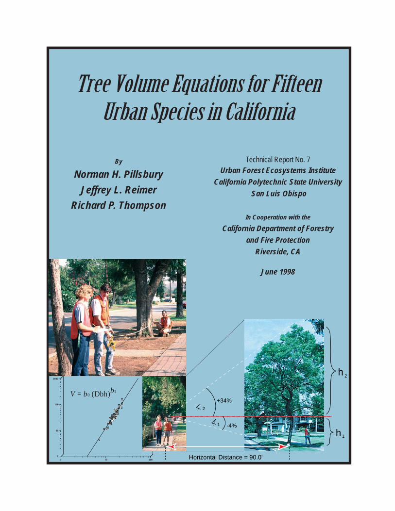
Technical Report No. 7Urban Forest Ecosystems Institute

California Polytechnic State University

San Luis Obispo

In Cooperation with the

California Department of Forestry

and Fire Protection

Riverside, CA

June 1998

Tree Volume Equations for FifteenUrban Species in California

V = b0 (Dbh)b1

1

1

2

2

Horizontal Distance = 90.0'

+34%

-4%

h

h

By

Norman H. Pillsbury

Jeffrey L. Reimer

Richard P. Thompson

1

10

100

1000

1 10 100

ii

Tree Volume Equations for Fifteen Urban Species in California

Technical Report No. 7Urban Forest Ecosystems Institute

California Polytechnic State University

San Luis Obispo

In Cooperation with the

California Department of Forestry

and Fire Protection

Riverside, CA

June 1998

Tree Volume Equations for FifteenUrban Species in California

V = b0 (Dbh)b1

1

1

2

2

Horizontal Distance = 90.0'

+34%

-4%

h

h

By

Norman H. Pillsbury

Jeffrey L. Reimer

Richard P. Thompson

1

10

100

1000

1 10 100

iv

Tree Volume Equations for Fifteen Urban Species in California

Table of Contents

Table of Contents ........................................................................................ ii

Acknowledgements .................................................................................... iii

Preface ................................................................................................... iv

I. Introduction ....................................................................................... 1

II. Overview and Goals of the Urban Forest Utilization Project ........... 2

Development of Tree Volume Equations ................................... 2

Development of Community Forest Inventories ....................... 2

Information Management for Budgeting & Product Devel. ...... 3

III. Study Criteria and Design ................................................................. 5

Selecting Communities with Urban Forestry Programs ............ 5

Species Selection ....................................................................... 8

IV. Procedures and Data Collection Methods ......................................... 15

Sample Size ............................................................................... 15

Geographic Stratification ........................................................... 15

Diameter Distribution ................................................................ 15

Tree Data Collected ................................................................... 15

V. Tree Volume Calculation ................................................................... 19

VI. Volume Equations .............................................................................. 23

VII. Tests of Equation Fit, Reliability and Measures of Accuracy ........... 25

Limitations of Equations ........................................................... 26

VIII. Application of Equations to an Independent Inventory..................... 29

IX. Summary and Conclusions ................................................................ 33

X. Literature Cited.................................................................................. 34

XI. Appendix ........................................................................................... 37

Calculating Tree Volume from a Volume Table ......................... 39

Local Volume Tables for Fifteen Urban Forest Species ............ 40

Standard Volume Tables for Fifteen Urban Forest Species ....... 41

ii

v

Tree Volume Equations for Fifteen Urban Species in California

Acknowledgements

The California Department of Forestry and Fire Protection and the Urban Forest

Ecosystems Institute at Cal Poly State University, San Luis Obispo have developed a partnership

to conduct an urban volume and biomass study for the communities of Anaheim, Pasadena,

Glendale, San Luis Obispo, Oakland, Monterey Peninsula, Sacramento, Modesto and Visalia,

California.

We would like to thank the following for their support and assistance with the project:

Mr. Eric Oldar, Urban Forester, California Department of Forestry and Fire Protection

Mr. Dave Neff, Resource Manager, California Department of Forestry and Fire Protection

Mr. Ron Morrow, Urban Forestry Manager, City of Anaheim

Mr. Douglas Nickels, Urban Fire Forester, City of Glendale

Mr. John Alderson, Parks & Forestry Administrator, City of Pasadena

Mr. Lamont Klecker, Parks & Forestry Project Manager, City of Pasadena

Ms. Jeannette Gonzales, Administrative Assistant, Cal Poly, San Luis Obispo

Mr. Tom Larson, Urban Forestry Consultant, Laguna Hills, California

Mr. Chris Rose, Forestry Student, Cal Poly, San Luis Obispo

Mr. Gary Mason, Urban Forestry Consultant, Berkeley, California

Mr. Robert Reid, Urban Forester, Monterey

Mr. Frank Ono, City Forester, Pacific Grove

Mr. Todd Martin, City Arborist, San Luis Obispo

Mr. Joe Newman, Urban Forester, Oakland

Mr. Gary Kelly, Director of Forest, Parks and Beach, Carmel

Mr. Chuck Gilstrap, Urban Forestry Supervisor II, Modesto

Mr. Allen Lagarbo, Arborist, Modesto

Mr. Martin Fitch, Parks Superintendent, Sacramento

Mr. Dave Pendergraft, Arborist, Visalia

This project was supported by the California Department of Forestry and Fire Protection,

the Urban Forest Ecosystems Institute, Cal Poly State University, San Luis Obispo, and through

a McIntire-Stennis Forestry Research grant.

iii

vi

Tree Volume Equations for Fifteen Urban Species in California

Preface

The call for improved management and sustainability of California’s urban forests has

been heard.

This call has led to a number of projects that have been recently completed, while others

are waiting to be implemented. Recently completed efforts include the “One California Forest”

brochure that has been mailed to thousands of citizens, a public opinion survey documenting

attitudes and preferences of Californian’s toward urban forestry issues, two regional workshops

leading to development of an urban forestry strategic planning document for participating

communities, and a study identifying and evaluating the elements of sustainability in urban

forestry.

This study describes three levels of forest inventory, and provides the basic volume

prediction models and inventory techniques needed to take the next step toward sustainability

of the urban forest resource.

iv

1

Tree Volume Equations for Fifteen Urban Species in California

For an inventory to serve as a manage-ment tool, it should describe the structure,composition and “volumes” of the urbanforest with reasonable accuracy. To achievethese results, data must be collected on treesize (i.e., diameter at breast height, and totalheight), and age (date planted) in addition tospecies, location, and health or damage rating.Data on maintenance activities, costs andtiming would make the inventory even moreuseful. Because developing such comprehen-sive inventories requires a considerableinvestment in time and resources, standardizedmethods are needed to assist urban foresters indata collection, analysis and inventory assess-ment. The purpose of this report is to assisturban foresters in developing a comprehensiveinventory.

A special section is presented on pages 2and 3 for the reader to understand how thisstudy fits into the multi-year Urban ForestUtilization project and its role in enhancingthe sustainability of urban forests.

Modified versions of this report werepresented as a video titled “Cal Poly UrbanForest Sustainability Project” (Pillsbury,Reimer and Thompson), and a paper titled“Tree volume equations for ten urban speciesin California” (Pillsbury and Reimer) at theSymposium on Oak Woodlands: Ecology,Management and Urban Interface Issues(March 21, 1996 Cal Poly, San Luis Obispo).It was also reported in the Symposium Pro-ceedings (Technical editors: Pillsbury, N., J.Verner, and W. D. Tietje 1997).

Cities throughout California are facingtremendous challenges in funding and sustain-ing urban forestry programs. Some of thecostliest operations are tree care and removal,and disposing of wood residues. Urbanforesters can no longer afford to operate in amanner that treats urban forest wood residuesas a costly disposal problem. Recycled usesfor these wood residues could generate signifi-cant savings in handling and landfill costs,costs that are growing rapidly. Even moreattractive is the prospect that these woodresidues could actually generate net revenuesif markets for energy and high quality woodscould be identified and developed.

Perhaps the most current example show-ing use of green waste is discussed in a reporttitled: “Greenwaste Reduction ImplementationPlan (GRIP), an Urban Forestry BiomassUtilization Project” prepared by IntregratedUrban Forestry, Inc. in conjunction with CalPoly, San Luis Obispo (Larson and O’Keefe1996).

To move urban forestry programs fromthe costly status quo to a more sustainablestate, where wood residues are valued, a morecomprehensive inventory of the urban forest isrequired. Many communities have developeda “street tree inventory” which typicallydescribes the location and health condition oftrees by species. Such an inventory is animportant step in understanding the composi-tion of the urban forest. However, much moreinformation is needed to begin managing theurban forest in a sustainable fashion.

Tree Volume Equations for Fifteen Urban Species inCalifornia

I. Introduction

2

Tree Volume Equations for Fifteen Urban Species in California

Overview and Goals of theUrban Forest Utilization Project

Phase I - Development of TreeVolume Equations

The first phase involves biometricstudies to enable the urban forester topredict the volume of various treespecies for the future sustainable urbanforests. Detailed measurements aremade of sample trees in order to createa statistical model for eachpredetermined species. Volumeprediction equations are developed.

It is this phase that is presented inthis report. Results of Phases II and IIIwill be reported separately.

Phase II - Development ofCommunity Forest Inventories

Using the prediction models fromPhase I, cities can expand their currentstreet tree inventory and begin to create

The goal of this project is to conduct a series of volume studies of the major urban forestspecies to further the development of management inventories in each California city for thepurpose of promoting sustainable urban forests. To accomplish this goal, the project has beenbroken down into three phases:

1001 011

10

100

1000

Tree Diameter (inches)

Tre

e V

olum

e (c

ubic

fee

t)

a management inventory. Collecting data ontree diameter in addition to data on species,location, planting date, and tree condition isall that is necessary for estimating total inven-tory. Other data on maintenance activities,

tree heights, usefullife, growth rate,value and productutilization are neededto create a compre-hensive inventory. Acomprehensiveinventory can be usedto manage by rotationand develop productand sustainablebudgets (see PhaseIII).

Figure 1. Tree prediction equation for Chinese Elm.

Figure 2. Streettree inventory forMonterey County.

3

Tree Volume Equations for Fifteen Urban Species in California

Phase III - Information Management for Budgeting & Product Development

As urban forest managementinventories are established, awhole range of managementfunctions can be enhanced andnew opportunities explored.Cities can use such inventories todesign the urban forest tonormalize its species compositionand structure; better plan andorganize planting, care, trimmingand removal activities; andestablish new uses and marketsfor the regularized wood residuesflows. Combined with a GISdatabase, new ways ofintegrating the urban forest intothe city infrastructure andinteracting with the public can bedeveloped.

Management Information System

Inventory GIS

Plans

Budgets

Maps

Data Collection

Sustained (Rotational)Management

Biomass &Wood Markets

City GovernmentPlanning

PubicRelations

Street TreeInventory

ManagementInventory

ComprehensiveInventory

Damage

Condition

Location

Species

Volume by size class

Volume

Tree height

Basal area

Tree dbh

Damage

Condition

Location

Species

Rotation plan

Value

Product utilization

Growth rate

Age

Volume by size class

Volume

Tree height

Basal area

Tree dbh

Damage

Condition

Location

Species

Increased Management Capabil i ty

Da

ta&

Info

rma

tio

n

Figure 4. The potential to manage theurban forest in a sustainable mannersubstantially increases when specific treedata is collected and managed. Boldface items are required, plain text isoptional, to achieve each inventory level.

Figure 3. Multiple products of the urban forest are possible witha comprehensive inventory.

4

Tree Volume Equations for Fifteen Urban Species in California

5

Tree Volume Equations for Fifteen Urban Species in California

As discussed earlier, the objective of thisstudy is to develop equations that can be usedto predict or estimate tree volume for urbanforest species from various geographicalregions and communities in California. Thefollowing sampling design was used todevelop prediction equations for urban forestspecies in California.

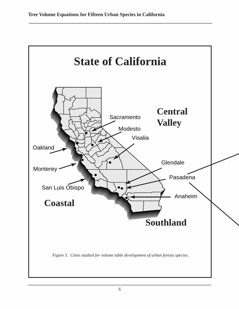
Selecting Communities with UrbanForestry Programs

California was first divided into threebroad geographic regions, Southland, Coastaland the Central Valley (see Figure 5). Therationale for this initial stratification is toensure that species selected represent majorclimatic conditions found in thestate.

Three communities in eachgeographic region wereidentified that could benefit froman evaluation of the volumepotential of their urban forest.Communities were selectedbased on the criteria shown inTable 1 (Pillsbury and Thompson1995).

III. Study Criteria and Design

Table 1. Criteria for selecting communitiesfor urban forest sampling

1. The community must have an active urbanforestry program. The program must beprominently visible in the city’sorganizational structure, and have anidentified urban forester in charge.

2. The urban forestry program must be able todemonstrate a commitment to long-termurban forest development and be on the roadto sustainability. The four core elements ofsustainability are: species selection anddiversity, inventory and landscape planning,tree care and wood utilization, and publicrelations and support. For more informationon sustainability, see “The Elements of

A 53’ tall Acacia, with a29.9” dbh, was measuredin the coastal town ofCarmel.

6

Tree Volume Equations for Fifteen Urban Species in California

Glendale

Pasadena

Anaheim

San Luis Obispo

Monterey

Oakland

Sacramento

Modesto

Visalia

Southland

Coastal

Figure 5. Cities studied for volume table development of urban forests species.

State of California

CentralValley

7

Tree Volume Equations for Fifteen Urban Species in California

Sustainability in Urban Forestry” byThompson, Pillsbury and Hanna (1994).

3. The community must at least have thebeginnings of a street tree inventory. Theinventory must be computer-based and beaccessible for future studies discussed inPhase II (on page 2), Development ofCommunity Forest Inventories.

4. Within each geographic area of the state,urban foresters must agree on the species thatwill be sampled.

5. Communities having large, old trees that arefacing removal in the next 5-10 years werefavored because prediction equations wouldbe more relevant in the near term.

Communities that were selected for studyare shown in Table 2. Clearly many othercommunities could be included in the sample,and as the need and support arises, they can beadded. The intent here is to provide specificinformation on selected communities fromdifferent parts of California rather thanintensively sample in one or two cities. It isour hope that the value of these results willencourage equation development of additionalspecies in the same or other communities.However, the information collected for thecommunities that were sampled will allow“preliminary” estimates of volume for othercities as well. See the discussion in sectionVII on equation use and limitations.

Sector 4

Sector 3

Sector 2Sector 1

Figure 6. Each city was stratified intosectors to ensure that all areas wereincluded in the sample.

8

Tree Volume Equations for Fifteen Urban Species in California

Species Selection

Five species in each geographic regionwere selected for study. Species were selectedbased on the criteria presented in Table 3.

Table 3. Criteria for selecting tree species

1. Species had to be well represented in eachcommunity of the geographic region. Thiswas evaluated by urban foresters and fromstreet tree inventories.

2. Species with a high probability for removalin the next decade were given higher priority.We decided that the prediction equationsdeveloped in this study should representspecies most likely to be harvested in thenear future, rather than species recentlyplanted that will not be removed soon.

3. Species that attain larger sizes were favoredin the selection process, as they providegreater volumes for use and represent greatersavings of disposal costs.

4. Species were favored for selection that werejudged to be of higher wood quality, andvalue.

5. Five species were selected from each geo-graphic region with the restriction thatspecies not be duplicated among regions.Developing equations for the same species indifferent regions will be considered in thefuture; the focus of this study is to gathervolume information on a greater number ofspecies rather than on regional differencesthat might exist.

6. Species were ranked lower on the list ifequations were available from other studies,even if the studies did not include trees froman urban environment. An example of this iscoast live oak (Quercus agrifolia) which hasbeen reported in several publications includ-ing Pillsbury and Kirkley (1984).

The selection process involved muchdiscussion among the authors and urbanforesters from these communities, and manyadditional species were considered. Thespecies selected, by geographic region, are

Table 2. Communities selected for volume sampling.

Region Community Year of SampleSouthland Anaheim 1994

Glendale 1994Pasadena 1994

Coastal San Luis Obispo 1995Monterey Peninsula 1995Oakland 1995

Central Valley Visalia 1996Modesto 1996Sacramento 1996

9

Tree Volume Equations for Fifteen Urban Species in California

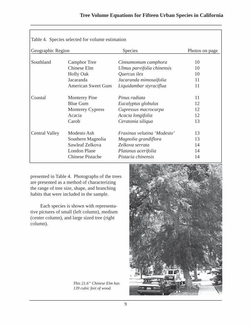
Table 4. Species selected for volume estimation

Geographic Region Species Photos on page

Southland Camphor Tree Cinnamomum camphora 10Chinese Elm Ulmus parvifolia chinensis 10Holly Oak Quercus ilex 10Jacaranda Jacaranda mimosaifolia 11American Sweet Gum Liquidambar styraciflua 11

Coastal Monterey Pine Pinus radiata 11Blue Gum Eucalyptus globulus 12Monterey Cypress Cupressus macrocarpa 12Acacia Acacia longifolia 12Carob Ceratonia siliqua 13

Central Valley Modesto Ash Fraxinus velutina ‘Modesto’ 13Southern Magnolia Magnolia grandiflora 13Sawleaf Zelkova Zelkova serrata 14London Plane Platanus acerifolia 14Chinese Pistache Pistacia chinensis 14

presented in Table 4. Photographs of the treesare presented as a method of characterizingthe range of tree size, shape, and branchinghabits that were included in the sample.

Each species is shown with representa-tive pictures of small (left column), medium(center column), and large sized tree (rightcolumn).

This 21.6” Chinese Elm has139 cubic feet of wood.

Tree Volume Equations for Fifteen Urban Species in California

10

Figure 7.1. Camphor Tree (Cinnamomum camphora) (l. to r., small, medium, large).

Figure 7.2. Chinese Elm (Ulmus parvifolia chinensis) (l. to r., small, medium, large).

Figure 7.3. Holly Oak (Quercus ilex) (l. to r., small, medium, large).

11

Tree Volume Equations for Fifteen Urban Species in California

Figure 7.4 Jacaranda (Jacaranda mimosaifolia) (l. to r., small, medium, large).

Figure 7.5 American Sweet Gum (Liquidambar styraciflua) (l. to r., small, medium, large).

Figure 7.6 Monterey Pine (Pinus radiata) (l. to r., small, medium, large).

Tree Volume Equations for Fifteen Urban Species in California

12

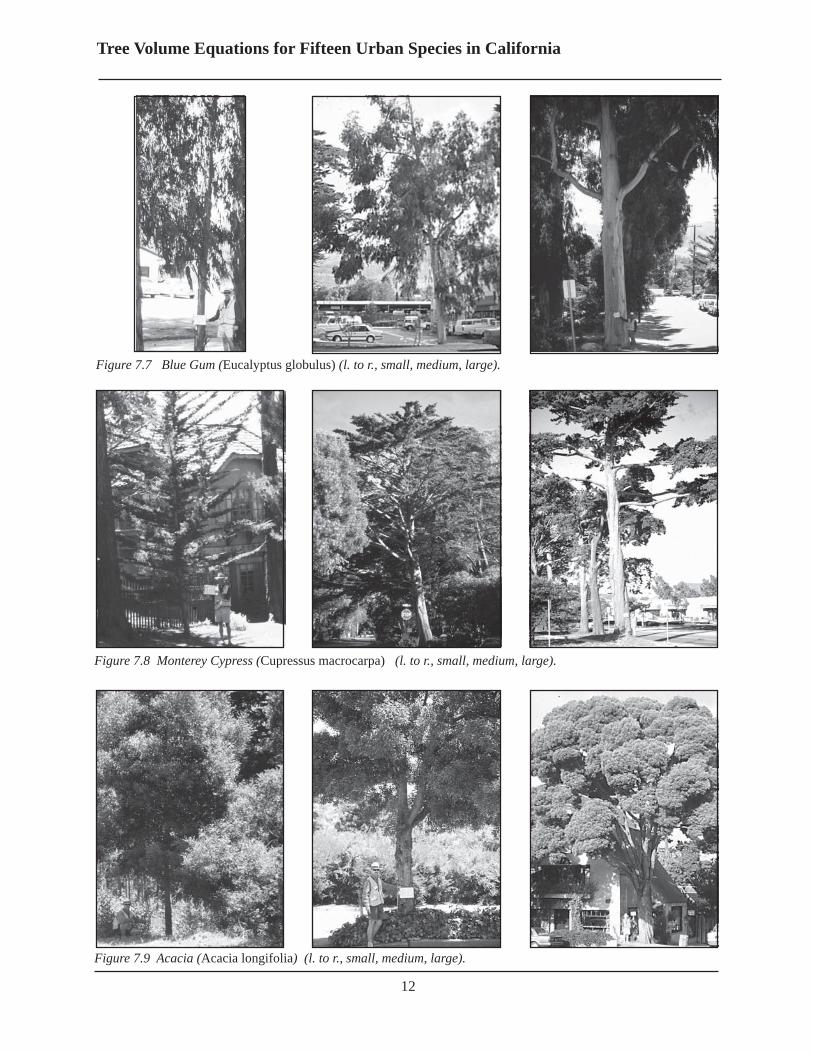
Figure 7.7 Blue Gum (Eucalyptus globulus) (l. to r., small, medium, large).

Figure 7.8 Monterey Cypress (Cupressus macrocarpa) (l. to r., small, medium, large).

Figure 7.9 Acacia (Acacia longifolia) (l. to r., small, medium, large).

13

Tree Volume Equations for Fifteen Urban Species in California

Figure 7.10 Carob (Ceratonia siliqua) (l. to r., small, medium, large).

Figure 7.11 Modesto Ash Fraxinus velutina ‘Modesto’ (l. to r., small, medium, large).

Figure 7.12 Southern Magnolia (Magnolia grandiflora) (l. to r., small, medium, large).

Tree Volume Equations for Fifteen Urban Species in California

14

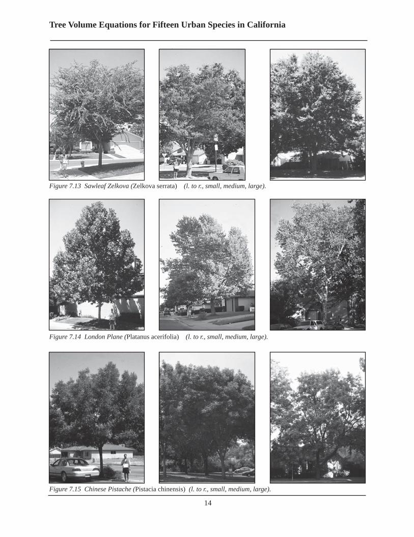
Figure 7.13 Sawleaf Zelkova (Zelkova serrata) (l. to r., small, medium, large).

Figure 7.14 London Plane (Platanus acerifolia) (l. to r., small, medium, large).

Figure 7.15 Chinese Pistache (Pistacia chinensis) (l. to r., small, medium, large).

15

Tree Volume Equations for Fifteen Urban Species in California

Sample Size

In similar volume studies 1 we found that

a sample size of 50 to 60 trees is the minimumnumber necessary to develop a statisticallyreliable estimate of the equation parameters.Based on these studies, a sample size of 50trees per species was adopted.

Geographic Stratification

Each geographic area is represented by 3cities or communities, and the number ofsample trees per species was equallyproportioned among their urban forests. Tofurther make certain that the sample designfully represents the geographic area, eachcommunity was stratified into 3 to 5 sectors ofapproximately equal area (in communitieswhere species were widely spread), and anequal number of sample trees were selectedamong sectors. This design, illustrated inFigure 6 for the City of Pasadena, ensured thatall sectors were sampled with similar intensity.

Diameter Distribution

In addition to sample size and geographicstratification concerns, the full range of treesizes found in the population was included inthe sample. Because volume is closelycorrelated to tree diameter, a graphicalaccounting of diameters was kept. As treeswere measured, their diameters were recordedin order to be certain that the full range of treesizes of each species was represented. In

addition, we checked each sector carefully tobe sure that representatives of the largest treeswere included in the sample.

Tree Data Collected

The data collected for each sample tree issummarized in Table 5. The variablescollected are listed and discussed below. Atree was defined as a evergreen or deciduousspecies 4.5’ or more tall.

Species. The common name wasrecorded on the data form. Trees havingmajor defects, unusually large damaged areas,or that were abnormally shaped or prunedwere not included in the sample. A review ofthe photographs displayed earlier will providea visual sense of the size, shape and conditionof sample trees.

Diameter at breast height. Diameter atbreast height outside bark (dbhob), wasmeasured with a diameter tape at a point 4.5’above the ground on the uphill side.Diameters are used in volume equationdevelopment. If the tree was leaning, the 4.5’was measured along the central stem axis. Fortrees that forked at breast height or lower, thetree was considered to be two trees; howevertrees of this type were not included in thesample unless specifically noted. If forkingoccurred just above breast height, a single dbhmeasurement was made below joint swelling.This means that dbh measurements could vary

1 Full references are provided in Section X; citations follow: Pillsbury, N. H. 1994; Pillsbury, N. H. and R. D. Pryor. 1994;Pillsbury, N. H. and D. R. Hermosilla. 1993; Pillsbury, N. H. and Pryor, R. D. 1992; De Lasaux, M. J. and Pillsbury, N. H. 1990;Pillsbury, N. H. and Pryor, R. D. 1989; Pillsbury, N. H., Standiford, R, Costello, L., Rhoades, T. and Regan (Banducci), P. 1989;and Pillsbury, N. H. and M. L. Kirkley. 1984.

IV. Procedures and Data Collection Methods

16

Tree Volume Equations for Fifteen Urban Species in California

Tree Location and Number. Trees werelocated by house and street address. If morethan one tree was growing at an address, thetrees were numbered sequentially followingthe direction of house numbers.

Photo and Sketch. Each tree wasphotographed with a 35 mm camera usingslide film. A placard was held to identify thetree. Also, as the segment data was collected,a sketch was drawn showing the relativelocation of each segment. This informationwas used for illustration and in a few caseswhen field notes were unclear.

anywhere from about 2’ to 4.5’ on the stem, oras high as 6’ if swelling biased dbhmeasurement at breast height. However theseexamples were few in number as almost allmeasurements were at 4.5’. It is importantthat use of the equations presented later in thisreport, follow these “rules” for greatestaccuracy.

Dob at 1 foot. Diameter outside bark wasalso measured at 1 foot to compute the volumeof the base segment. If butt swell was present,the measurement was taken where the treetaper was normal, usually no higher than 2feet. A diameter tape was used.

Total Height. Total tree height wasmeasured from the tree base on the uphill sideto the tip or tallest live portion of the crown(see Figure 8). Heights of leaning trees werecalculated using the vertical height to the treetip and the angle of the bole. Heights are usedin volume equation development.

Average Crown Diameter. Crowndiameter was determined by averagingmeasurements of the long axis with a diametertaken at 90°. Readings were taken with a 100’cloth tape. Data can be used to correlate withtree volume.

Number and Length of TerminalBranches. The last segment of a branch isreferred to as a “terminal branch” or “terminalsegment.” Terminal branches are defined asbeing 4” in diameter at the large end and zeroinches at the tip or small end. Terminalbranches or segments were included in thecalculation of tree volume. For each sampletree, 5 or 6 terminal branches were measuredfor length. In all cases, lengths wereconsistent within 2-3’, and an average wasobtained. The total number of terminalbranches was counted for each sample tree.

17

Tree Volume Equations for Fifteen Urban Species in California

Table 5. Data collected from urban tree species.

Characteristic Units Description

Used indevelopmentof equations

by the authors

Data theUrban

Foresterwill collect

A. Tree Information:

Species code A = AcaciaBG = Blue GumC = CarobCA = CamphorCE = Chinese ElmCP = Chinese PistacheHO = Holly OakJA = JacarandaLA = LiquidambarLP = London PlaneM = Southern MagnoliaMA = Modesto AshMC = Monterey CypressMP = Monterey PineZ = Sawleaf Zelkova

Yes Yes

Dbh inches Diameter at breast height, to thenearest 0.1 inch.

Yes Yes

Dob at 1’ inches Diameter to the nearest 0.1 inch. Yes No

Total Height feet Estimated total height to top ofterminal leader.

Yes Yes

Average CrownDiameter

feet Average of long and short axis, tothe nearest foot.

Yes No

Number andAverage Length of TerminalBranches

#, feet Count of the number of terminalbranches; average length determinedby measuring a sample for averageof long and short axis.

Yes No

B. Tree Identification Information:

Date Date of field measurement. Yes Yes

Photo Number Roll number and photo number Yes No

Tree Location andTree Number

Located by street address. If morethan one tree at the same address,trees were numbered in the directionof increasing address numbers.

Yes Yes

18

Tree Volume Equations for Fifteen Urban Species in California

A. When using percent.

1. First measure the horizontal distance from the treecenter to a point where you have a clear view of the tip.You may have to correct for slope on steep ground.Usually you will be between 60’ and 120’ from the tree.

2. With the clinometer measure the angle in percent toa) the tallest live point on the crown or tip (∠

2), and, b)

the tree base (∠1) uphill side.

3. Calculate the tree height as follows.

Total tree height+34 - -4

=( )[ ] ×

=90 0

10034 2

.. '

B. When using degrees.

1. First measure the horizontal distance from the treecenter to a point where you have a clear view of thetip. You may have to correct for slope on steepground. Usually you will be between 60’ and 120’from the tree.

2. With the clinometer measure the angle in degreesto a) the tallest live point on the crown or tip (∠

2),

and, b) the tree base (∠1) uphill side. Note that this

forms two right triangles.

3. Calculate the tree height as follows.The total angle is between the tree tip and the

tree base (uphill side), and is calculated by the topreading (∠

2) minus the base reading (∠

1), or (∠

2 - ∠

1).

Assume that ∠2 = +34%, and angle ∠

1 = -4%

(see picture above).

Then:

Figure 8. Determining tree height usingpercent and degrees.

Determining Tree Height. Total tree height (h1 + h2) is required to use the Standard volume equations andtables. A clinometer or abney level can be used to measure the vertical angle to the tree base and top in units ofpercent or degrees. The calculation procedure is different for the two types of units.

Total tree height = Total angle x Horizontal Distance

100

1

1

2

2

Horizontal Distance = 90.0'

+34%

-4%

h

h

Total tree height = Horizontal Distance x (tan ∠1 + tan ∠2)

= 90.0 x (tan 2° + tan 19° )

= 90.0 x 0.379248 = 34.1'

19

Tree Volume Equations for Fifteen Urban Species in California

Any level of use or managementinvolving the cutting and removal of urbantrees requires that accurate volume predictionequations be used. Volume equations can beused to determine tree removal volume,inventory, and for growth and yield studies.Reliable estimates of urban tree volumedepend, in part, on the accuracy of theequations developed. Also, they are morereliable within the geographic area fromwhich the field data were collected; the greaterthe distance from the collection area, the lessreliable.

We have been unable to find volumeequations developed from cities in California.Our search for equations included numerousurban foresters throughout the state, membersof the California Urban Forests AdvisoryCouncil, the California Department ofForestry and Fire Protection, the WesternUrban Forestry Research Center, PacificSouthwest Research Station, and faculty at CalPoly, San Luis Obispo and the University ofCalifornia, Berkeley.

Because equations for urban species donot exist, this study was initiated to developequations in the three geographic regions ofCalifornia discussed earlier.

For volume measurement, the branchingpattern was defined on a segment basis.Segment length and the diameters at each endwere measured using a Spiegel Relaskop(Pillsbury and Kirkley 1984, and others citedearlier). Segment length was determined fromcoordinates measured at both ends of eachsegment. Each tree was divided into segmentsbased on four criteria:

1. Segments were defined as the distance fromfork to fork in trees with very complex

branching pattern, such as segment 11 inFigure 9.

2. If a branch had a sweep or crook, segmentswere measured to obtain a straight log lengthsuch as in segments 3 and 5.

3. Segments were defined if abrupt changes intaper were apparent such as in segments 16and 17.

4. If a tree had an excurrent growth form, suchas Liquidambar, the maximum segmentlength measured was approximately 10 feet.

If swelling was present on the stem, acommon occurrence, relaskop diameterreadings were taken slightly above or belowthe abnormality. A two-step process was usedfor branches not growing vertically. First thevertical distance between the ends wascalculated based on relaskop coordinates.Secondly, an angle, to the nearest 1° fromhorizontal was measured with a clinometer,and segment length was computed. Segmentsgrowing less than 30° from horizontal weremeasured by projecting their length to theground and measuring it with a cloth tape heldparallel to the branch angle.

Cubic foot volume was calculated foreach tree using three equations fordetermining the cubic volume of a solid. Thestump (base segment) was treated as acylinder (equation 1), the tip was treated as acone (equation 2), and the remaining segmentswere treated as a paraboloid frustrum andSmalian’s formula was used (equation 3).

V = AuL [1]

V =L

3Ab( ) [2]

V. Tree Volume Calculation

20

Tree Volume Equations for Fifteen Urban Species in California

V LA Au b=

+( )2

[3]

where:

V = volume outside bark in cubic feet to

0-inch top,

Ab = cross sectional area outside bark at

base in square feet,

Au = cross sectional area outside bark at top

in square feet, and,

L = length of segment in feet.

Utilization Standards. Total tree volumeincludes the volume of all stem segments fromground level including terminal branches andbark. It does not include the volume of rootsand foliage. A spreadsheet formulated inMicrosoft Excel® (Figure 10) was developedto calculate individual tree volumes usingEquations 1-3. As there is no ready market forurban wood at this time, it is not known whatbranch or stem size will be needed by existingand developing wood manufacturingindustries. For example, some companiesmight be equipped to handle large diameter, 8’bolts, while others may operate in the small

Figure 9. Sample treeswere measured on asegment-by-segmentbasis to determinevolume. Numbers on treeindicate tree segments.

21

Tree Volume Equations for Fifteen Urban Species in California

Species: C E Location: 3190 Matero, Pasadena

Tree Number: 7 tree #1 Page: 1 of 1

Dob @ 1': 23.6 Date: 6 / 2 7 / 9 4

Dbh: 22.0

Total Height: 56.5 Average length (ft): 2 1 Ave Crown Dia.: 5 5

Number of small branches: 2 0

Roll/Photo No.: 0 2 - - 1 8

Vol of Total

Setup 1 2 3 4 Sm. Br. Volume

HD 33.0 Cu. Ft. = 12.22 12.57 23.86 27.18 5.69 18.25 99.77

% Vol = 12.24 12.60 23.92 27.24 5.70 18.29 100.00

27 H.D. 0.005454 Volume Volume Volume Volume Volume Volume

Setup Seg. Lower Lower Upper Upper Angle Direct Ave. Seg. 4.00 to 8.00 to 12.00 to 16.00 to All

No. No. Dob Coord. Dob Coord. (deg.) Length BA Length 7.99 in. 11.99 in. 15.99 in. 19.99 in. 20.00> in. Segments

1 1 23.6 23.6 1.0 3.04 1.00 3.04 3.04

1 2 23.6 22.0 3.5 2.84 3.50 9.94 9.94

1 3 22.0 -2.0 22.0 2.0 2.64 2.00 5.28 5.28

1 4 16.0 2.0 13.0 17.5 25.0 1.16 8.55 9.91 9.91

1 5 7.0 17.5 6.5 22.0 45.0 0.25 3.18 0.79 0.79

1 6 6.5 8.0 5.0 0.29 5.00 1.45 1.45

1 7 8.0 21.0 6.0 24.0 0.27 1.50 0.41 0.41

1 8 6.0 6.0 3.0 0.20 3.00 0.59 0.59

1 9 5.0 24.0 4.0 27.5 0.11 1.75 0.20 0.20

1 1 0 14.0 2.0 20.0 9.0 1.63 3.50 5.69 5.69

1 1 1 12.0 9.0 11.0 17.0 0.72 4.00 2.89 2.89

1 1 2 11.0 17.0 13.0 26.0 35.0 0.79 5.49 4.34 4.34

1 1 3 11.0 26.0 12.0 40.0 35.0 0.72 8.55 6.18 6.18

1 1 4 13.0 9.0 12.0 21.5 42.0 0.85 8.41 7.18 7.18

1 1 5 12.0 21.5 10.0 27.0 13.0 0.67 2.82 1.88 1.88

1 1 6 10.0 27.0 9.0 36.0 38.0 0.49 5.71 2.82 2.82

1 1 7 9.0 9.0 3.3 0.44 3.30 1.46 1.46

1 1 8 6.0 4.0 12.5 0.14 12.50 1.77 1.77

1 1 9 10.0 10.0 7.5 0.55 7.50 4.09 4.09

1 2 0 8.0 7.0 1.5 0.31 1.50 0.46 0.46

1 2 1 13.0 20.0 12.5 29.0 46.0 0.89 6.48 5.75 5.75

1 2 2 7.5 29.0 7.5 34.0 0.31 2.50 0.77 0.77

1 2 3 7.5 8.0 6.4 0.33 6.40 2.10 2.10

1 2 4 11.0 11.0 6.9 0.66 6.90 4.55 4.55

1 2 5 7.5 4.0 14.0 0.20 14.00 2.76 2.76

1 2 6 6.0 4.0 6.0 0.14 6.00 0.85 0.85

1 2 7 6.0 48.0 4.0 54.0 0.14 3.00 0.43 0.43

Figure 10. Spreadsheet showing cubic foot volume calculations.

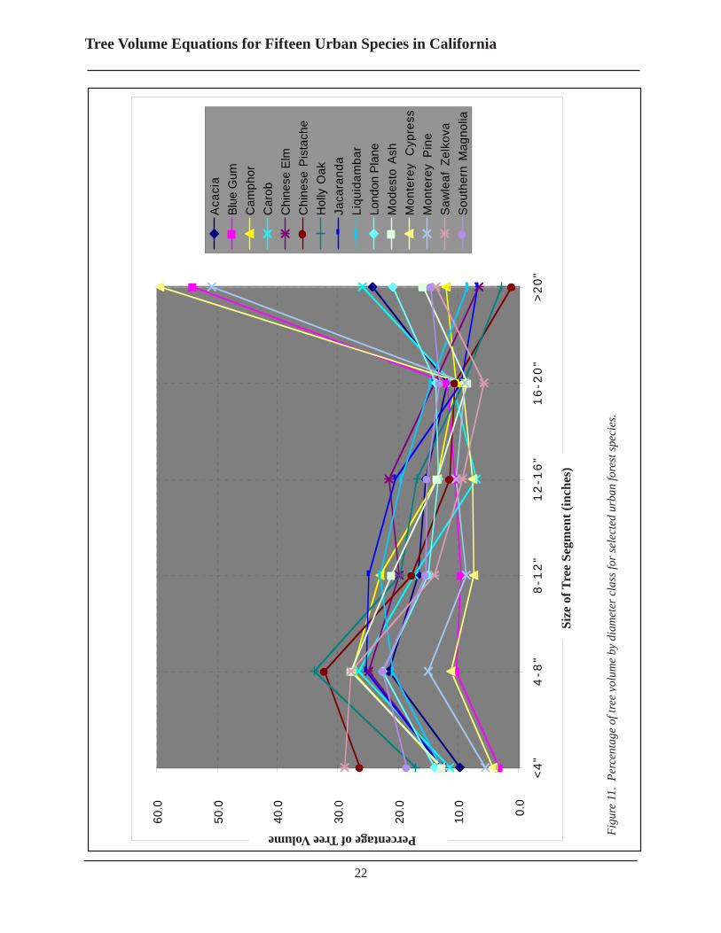
mulching market. In order to provideestimates for a variety of uses, the spreadsheetwas created to calculate wood volume in thefollowing diameter size classes: less than 4”,4-8”, 8-12”, 12-16”, 16-20”, greater than 20”as well as total volume. The average diameterof each segment was used to determine itsdiameter class. Further, these size classeswere set as variables, and can be changed toobtain volume proportions based on differentdiameter groupings. For instance, if one were

interested in firewood potential, the volumesof all segments in the 4-8” and 8-12” diameterclasses would be combined.

Based on field measurements, theaverage percent volume for the segmentdiameter classes discussed above are shown inFigure 11.

22

Tree Volume Equations for Fifteen Urban Species in California

Fig

ure

11.

Per

cent

age

of tr

ee v

olum

e by

dia

met

er c

lass

for

sele

cted

urb

an fo

rest

spe

cies

.

0.0

10.0

20.0

30.0

40.0

50.0

60.0

<4

"4

-8"

8-1

2"

12

-16

"1

6-2

0"

>2

0"

Aca

cia

Blu

e G

um

Cam

phor

Car

ob

Chi

nese

Elm

Chi

nese

Pis

tach

e

Hol

ly O

ak

Jaca

ran

da

Liq

uid

am

ba

r

Lond

on P

lane

Mod

esto

Ash

Mo

nte

rey

Cyp

ress

Mo

nte

rey

Pin

e

Saw

leaf

Zel

kova

Sou

ther

n M

agno

lia

Size

of T

ree

Segm

ent

(inc

hes)

Percentage of Tree Volume

23

Tree Volume Equations for Fifteen Urban Species in California

Ht. = total tree height in feet, and,b

i= regression coefficients.

Simple and multiple regression analysis(equations 4 and 5, respectively) was used todevelop the volume prediction equations(Tables 6 and 7). A logarithmictransformation of volume, dbh, and height wasused to equalize the variation about theregression line, and linearize a non-linearfunction so that ordinary least squaresregression can be preformed. The data wereconverted to the logarithmic form to computethe regression coefficients b

0, b

1, and b

2 . This

is the normal procedure when fitting nonlineartree volume equations because the logarithmicforms tends to reduce variance inhomogeneous samples (Husch et al. 1982).

From these equations, local and standardvolume tables were developed and arepresented in the Appendix.

Two types of equations are commonlyused to predict tree volume, local andstandard volume equations. Local volumeequations use one variable, diameter at breastheight (dbh) to estimate tree volume, while astandard volume equation uses both dbh andheight. Including height in the equationgenerally provides a better estimate as it helpsaccount for soil, climate and some culturalvariations. Because not all street treeinventories include height, both types ofequations are presented here to provideflexibility for the user.

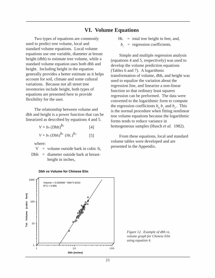
The relationship between volume anddbh and height is a power function that can belinearized as described by equations 4 and 5.

V = b0 (Dbh)b1 [4]

V = b0 (Dbh)b1 (Ht.)b2 [5]

where:V = volume outside bark in cubic ft,

Dbh = diameter outside bark at breast-height in inches,

VI. Volume Equations

Figure 12. Example of dbh vs.volume graph for Chinese Elmusing equation 4.

1001 011

10

100

1000

Dbh vs Volume for Chinese Elm

Dbh (inches)

To

t V

olu

me

(c

ub

ic

fee

t)

Volume = 0.028408 * Dbh^2.6410R^2 = 0.905

24

Tree Volume Equations for Fifteen Urban Species in California

Table 6--Local volume equations for selected urban forest speciesAverage PercentPercent Aggregate Eqn.

Species Equation Adj. R2 N SE Deviation Difference No.Blue Gum Vol (cf) = 0.055113 (dbh2.436970) 0.968 50 1.27 18.6 0.6 6

Acacia Vol (cf) = 0.048490 (dbh2.347250) 0.938 50 1.24 15.8 -3.0 7

Monterey Pine Vol (cf) = 0.019874 (dbh2.666079) 0.969 50 1.27 18.9 -1.7 8

Monterey Cypress Vol (cf) = 0.035598 (dbh2.495263) 0.980 50 1.23 15.7 1.9 9

Carob Vol (cf) = 0.066256 (dbh2.128861) 0.910 50 1.29 18.9 -2.3 10

Camphor Vol (cf) = 0.031449 (dbh2.534660) 0.970 50 1.17 12.5 -1.2 11

Chinese Elm Vol (cf) = 0.028530 (dbh2.639347) 0.903 50 1.22 16.6 -2.3 12

Holly Oak Vol (cf) = 0.025169 (dbh2.607285) 0.938 50 1.24 17.0 -1.3 13

Jacaranda Vol (cf) = 0.036147 (dbh2.486248) 0.949 49 1.19 13.9 0.0 14

Liquidambar Vol (cf) = 0.030684 (dbh2.560469) 0.979 50 1.15 10.5 -0.5 15

Modesto Ash Vol (cf) = 0.022227 (dbh2.633462) 0.940 50 1.29 20.4 -4.5 16

Sawleaf Zelkova Vol (cf) = 0.021472 (dbh2.674757) 0.969 50 1.21 15.7 -0.7 17

Chinese Pistache Vol (cf) = 0.019003 (dbh2.808625) 0.958 49 1.24 17.3 -0.3 18

Southern Magnolia Vol (cf) = 0.022744 (dbh2.622015) 0.958 50 1.24 15.6 0.8 19

London Plane Vol (cf) = 0.025170 (dbh2.673578) 0.965 50 1.22 16.2 -3.3 20

Note: For an explanation of terms used here, see the discussion in the text.

Table 7--Standard volume equations for selected urban forest speciesAverage PercentPercent Aggregate Eqn.

Species Equation Adj. R2 N SE Deviation Difference No.Blue Gum Vol (cf) =0.003089 (dbh2.151822)(ht0.835731) 0.983 50 1.19 10.9 -1.0 21Acacia Vol (cf) = 0.014058 (dbh2.186485)(ht0.467357) 0.976 50 1.14 14.5 -2.7 22Monterey Pine Vol (cf) = 0.005325 (dbh2.226808)(ht0.668993) 0.979 50 1.22 16.0 -1.1 23Monterey Cypress Vol (cf) = 0.005764 (dbh2.260353)(ht0.630129) 0.989 50 1.16 11.9 2.2 24Carob Vol (cf) = 0.008573 (dbh1.795854)(ht0.926668) 0.933 50 1.24 17.8 -1.4 25Camphor Vol (cf) = 0.009817 (dbh2.134803)(ht0.634042) 0.976 50 1.15 10.9 -1.3 26

Chinese Elm Vol (cf) = 0.010456 (dbh2.324812)(ht0.493171) 0.915 50 1.21 14.8 -1.9 27

Holly Oak Vol (cf) = 0.004307 (dbh1.821580)(ht1.062691) 0.976 50 1.15 10.4 0.3 28

Jacaranda Vol (cf) = 0.011312 (dbh2.185780)(ht0.548045) 0.956 49 1.17 12.7 0.1 29

Liquidambar Vol (cf) = 0.011773 (dbh2.315815)(ht0.415711) 0.982 50 1.13 9.2 -0.6 30

Modesto Ash Vol (cf) = 0.001287 (dbh1.762964)(ht1.427822) 0.978 50 1.17 12.6 -1.3 31

Sawleaf Zelkova Vol (cf) = 0.006664 (dbh2.363178)(ht0.551904) 0.975 50 1.18 14.2 0.5 32

Chinese Pistache Vol (cf) = 0.002921 (dbh2.191572)(ht0.943669) 0.969 49 1.20 15.2 0.4 33

Southern Magnolia Vol (cf) = 0.004486 (dbh2.070408)(ht0.845627) 0.973 50 1.19 13.2 0.5 34

London Plane Vol (cf) = 0.010425 (dbh2.436420)(ht0.391682) 0.966 50 1.21 16.0 -2.6 35Note: For an explanation of terms used here, see the discussion in the text.

25

Tree Volume Equations for Fifteen Urban Species in California

There is no one measure of the adequacyof volume equations. We examined several ofthe more common tests to determine theoverall fit and reliability of the equations. InTables 6 and 7, several statistics are providedthat helps the reader understand the relativeprecision of the relationships that have beendeveloped. The statistical terms used in thissection are further discussed in basic statisticaltexts such as Draper, N. R. and H. Smith(1981) and Snedecor, George W. and WilliamG. Cochran (1967).

Error and Outlier Analysis. Concurrentwith the development of the predictionequations, the data were carefully checked todetermine if measurement or recording errorswere present. We developed computerprograms to “look” for possible errors indiameter, height, and tree segment data. Treevolumes were checked by examining thestandardized residual calculated for each tree.Even if a tree showed an unusual relationshipbetween the dbh and height values andvolume, the tree was checked against thesketch and photograph for legitimacy. Afterall checks were performed, only one tree wasremoved from the data set based on thesetests.

Measures of reliability and accuracy arediscussed in detail in the sidebar.

Other Measures. In addition to thereliability tests previously discussed in thesidebar, several other tests were conducted.These included analysis of the F-value, theroot mean squared error (another measure ofthe residual variation), and plots of residualsto check for nonlinearity, and nonconstanterror variance. In no case did we find reasonto believe a problem in the database existed.

VII. Tests of Equation Fit, Reliability and Measures of Accuracy

Measures of reliability and accuracy

Coefficient of Determination. The term R2, or the

Coefficient of Determination, is provided in Tables 6and 7 to show the proportion or percentage of thevariation about the average sample volume that isexplained by the regression. In previous work wehave found that equations with R

2 values of .90 (90%)

or higher are considered very good and make goodpredictors. All equations developed for this study hadR-squares between 0.90 and 0.98.

Standard Error of the Estimate. SE is the abbrevia-tion used in these tables for this measure of reliability.The standard error of the estimate indicates, involume units, the error associated with the meanvolume of each species. For example, the standarderror for the Camphor standard volume equation(Table 7) is 1.15, or 1.15 cubic feet. In studies citedearlier, the standard error varied between 1.00 - 1.40,indicating that these tree volume equations have thehigh level of precision desired.

Average Percentage Deviation. The average percent-age deviation measures the extent to which theindividual observations of sample tree volume deviatefrom the regression surface. This percentage gives anidea of the amount by which any single calculatedvalue (or value read from a volume table) will varyfrom the actual value. It is calculated by:

Average percentage deviation =

Va - Ve x 100

Ve

∑ ÷ N [36]

where Va is the actual volume, Ve is the equation ortable volume, and N is the number of sample trees.These values, shown in Table 8, range from about 9%to 19%. For example, using the local volumeequation (LVE) for Camphor, the volume of anindividual tree is expected to deviate from the actualvolume by 12.5%. In practice these percent differ-ences can be higher as equations are applied to newindividuals; in extreme cases as high as 30-40%. Forthis reason, volume prediction equations are usuallynot meant to be used on a tree by tree basis exceptwhere only a rough estimate is needed.

continued

26

Tree Volume Equations for Fifteen Urban Species in California

Limitations of Equations

It must be emphasized, that the measuresof reliability and accuracy presented aboveonly pertain to the accuracy of the equationsin the context of the data used in theirconstruction. Despite the efforts of theauthors to develop and implement a soundsampling design, and to carefully evaluate theresults, there is still no guarantee that theseequations and tables will always apply equallywell to an independent sample. However, pastexperience has shown that equationsdeveloped by these rigorous measures willperform well, usually within 10-12%, if fieldprocedures follow the methods outlined in thisreport. When a more accurate estimate isrequired, say in the case of a sale or purchaseof standing trees, the equations (or tables)should be checked against the measuredvolumes of a representative sample of treesobtained from the area of interest.

Volume equations will best represent thecommunities where the data was originallycollected. To apply the equations in adifferent portion of the state runs the risk ofunacceptable errors (Pillsbury, McDonald,Simon 1995). The question of “how well willthey do” in a new environment cannot beanswered without additional study. Oftenequations are used out of their geographic areasimply because they are the “best” equationsavailable. Clearly the user takes theresponsibility for the results.

There are two ways that people useequations in different areas. First, they areoften used “as is,” however, the user shouldalways indicate that the equations were notdeveloped in that area, that the results are“preliminary” or “ball park”, and that thedegree of error is unknown. A more desirableapproach is first, to select 15 or 20 trees per

species that span the range of diameters,secondly, to carefully measure them by theapproach discussed here, or if cut, useequations 1,2 and 3 to estimate their volume,and last, to develop a ratio of the total volumefrom the new sample to the total volumeproduced by the equations (or tables). Theratio is used to adjust volumes calculatedusing the equations in the new area.

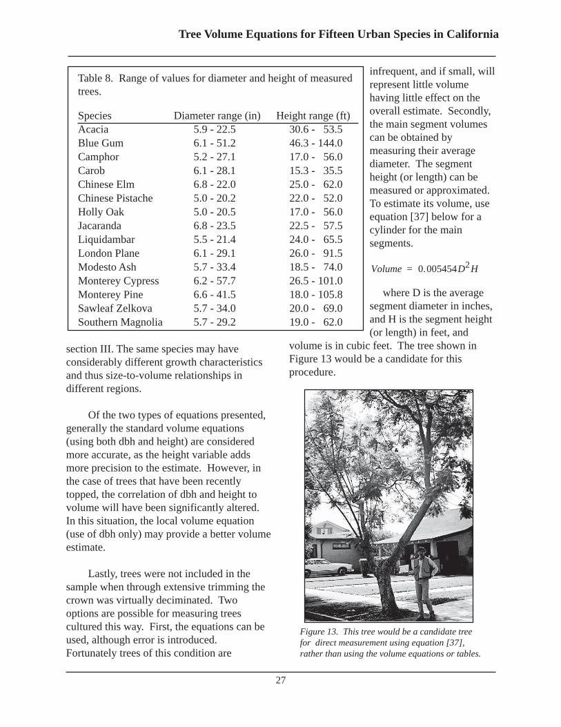
Significant errors can also result if theprediction equations are used to estimatevolume of trees whose dbh and height valuesare outside the sample range. For best results,tree sizes should fit into the range of datacollected and extrapolation avoided. Table 8shows the range of diameters and tree heightsmeasured for each species. Errors may alsooccur if the tree shape or form deviatessignificantly from the portraits shown in

Measures of reliability and

accuracy -- continued

Percent Aggregate Difference. Theaggregate difference approach isconsidered to be a better indicator ofreliability because most users areinterested in the accuracy of the volumeof a large number of trees rather thanindividual tree volumes. Aggregatedifference is the difference between thesum of the predicted and the sum of theactual volumes for a given sample.When applied to the sample trees in thisstudy, the percents ranged from 0.0% to3.0% (plus or minus), Table 8. Thesevalues compare favorably with previousstudies, including, a range of 0.3% -2.7% for redwood (Pillsbury and DeLasaux 1990), and 2.1% - 5.8% for 13California hardwoods (Pillsbury andKirkley 1984).

27

Tree Volume Equations for Fifteen Urban Species in California

section III. The same species may haveconsiderably different growth characteristicsand thus size-to-volume relationships indifferent regions.

Of the two types of equations presented,generally the standard volume equations(using both dbh and height) are consideredmore accurate, as the height variable addsmore precision to the estimate. However, inthe case of trees that have been recentlytopped, the correlation of dbh and height tovolume will have been significantly altered.In this situation, the local volume equation(use of dbh only) may provide a better volumeestimate.

Lastly, trees were not included in thesample when through extensive trimming thecrown was virtually deciminated. Twooptions are possible for measuring treescultured this way. First, the equations can beused, although error is introduced.Fortunately trees of this condition are

infrequent, and if small, willrepresent little volumehaving little effect on theoverall estimate. Secondly,the main segment volumescan be obtained bymeasuring their averagediameter. The segmentheight (or length) can bemeasured or approximated.To estimate its volume, useequation [37] below for acylinder for the mainsegments.

Volume = 0.005454D2H

where D is the averagesegment diameter in inches,and H is the segment height(or length) in feet, and

volume is in cubic feet. The tree shown inFigure 13 would be a candidate for thisprocedure.

Figure 13. This tree would be a candidate treefor direct measurement using equation [37],rather than using the volume equations or tables.

Table 8. Range of values for diameter and height of measuredtrees.

Species Diameter range (in) Height range (ft)Acacia 5.9 - 22.5 30.6 - 53.5Blue Gum 6.1 - 51.2 46.3 - 144.0Camphor 5.2 - 27.1 17.0 - 56.0Carob 6.1 - 28.1 15.3 - 35.5Chinese Elm 6.8 - 22.0 25.0 - 62.0Chinese Pistache 5.0 - 20.2 22.0 - 52.0Holly Oak 5.0 - 20.5 17.0 - 56.0Jacaranda 6.8 - 23.5 22.5 - 57.5Liquidambar 5.5 - 21.4 24.0 - 65.5London Plane 6.1 - 29.1 26.0 - 91.5Modesto Ash 5.7 - 33.4 18.5 - 74.0Monterey Cypress 6.2 - 57.7 26.5 - 101.0Monterey Pine 6.6 - 41.5 18.0 - 105.8Sawleaf Zelkova 5.7 - 34.0 20.0 - 69.0Southern Magnolia 5.7 - 29.2 19.0 - 62.0

28

Tree Volume Equations for Fifteen Urban Species in California

29

Tree Volume Equations for Fifteen Urban Species in California

The following discussion outlines thesteps necessary to conduct a field inventoryfor volume and an office estimate for treesscheduled for removal from your urban forest.

Your field crews have input street treeinventory data that shows 200 trees arescheduled for removal in the northeast part ofyour community during the next three years.The species involved are those for whichequations have been developed. (If equationswere not available for some species, whatwould you do? See discussion on page 27,column 2).

Rather than cut and haul the wood to thelandfill over a three year period, you decide tocontact two area-wide hardwoodmanufacturers, and obtain bids on the wood.This strategy, in addition to providing revenuefor your urban forestry program, will alsoreduce the time frame to one summer, andrelieve the extra burden from your fullycommitted crews. The purchasers and youagree to sell the wood based on a measure ofthe cut trees, however, to provide a reasonableestimate of cubic foot quantity available forthe bid, you perform the following analysis.(If the conditions of sale were based on thevolume estimate of the standing trees, whatimportant step would come first? See the“Limitation of Equations” discussion on page26).

Field verification: A quick verification ofthe information in your street tree inventory isneeded. A crew is dispatched to check andupdate the database for location, species, anddiameter, and if time is available, for total treeheight. Field equipment needed, is a diametertape, clinometer, and a 100’ tape. A writtennotice is left on the nearest premise advising

VIII. Application of Equations to an Independent Inventory

residents of the project.Diameter and height measurements

should follow the methods discussed insection IV. Total tree height is calculated asshown in Figure 8.

Office calculations: An example of howto obtain tree volume estimates for theequations and tables is presented here. Thedata should be kept separate by species.

Use of Volume Equations. A ChineseElm was measured and found to have a 16.8”dbh and a total height of 54.2’. Substituteyour data into equation [22] a standard volumeequation from Table 7, as follows:

1. Vol (cf) = 0.010456450 (dbh 2.324812059)

(ht 0.493171357)

2. Vol (cf) = 0.010456450 (16.8 2.324812059)

(54.2 0.493171357)

3. Vol (cf) = 0.010456450 x 705.690 x 7.164= 52.9 cubic feet

If height data was not collected, be sureto use the local volume equation (number [7]from Table 6), as follows:

1. Vol (cf) = 0.028530182 (dbh 2.639347250)

2. Vol (cf) = 0.028530182 (16.8 2.639347250)3. Vol (cf) = 0.028530182 x 1714.023 = 48.9

cubic feet.

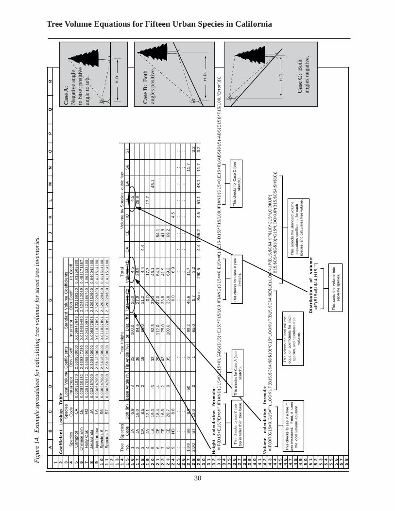
This approach is greatly simplified bysetting up a spreadsheet with the regressioncoefficients referenced as absolute, and thetree data referenced as relative. See Figure 14for an example using Microsoft Excel®.

30

Tree Volume Equations for Fifteen Urban Species in California

1 2 3 4 5 6 7 8 9 10

11

12

13

14

15

16

17

18

19

20

21

22

23

24

25

26

27

28

29

30

31

32

33

34

35

36

37

38

39

40

41

42

43

44

45

46

47

48

49

50

51

52

53

54

55

56

57

58

AB

CD

EF

GH

IJ

KL

MN

OP

QR

Co

eff

icie

nt

Lo

ok

up

T

ab

leS

peci

esLo

cal

Vol

ume

Coe

ffic

ient

sS

tand

ard

Vol

ume

Coe

ffic

ient

sS

peci

esC

ode

Inte

rce

pt

Dbh

Coe

ffIn

terc

ep

tD

bh C

oeff

Ht

Coe

ffC

amph

orC

A0

.00

03

18

17

02

.53

05

00

00

00

.00

99

47

64

82

.13

21

69

20

00

.63

25

08

80

0C

hine

se E

lmCE

0.0

28

53

01

82

2.6

39

34

72

50

0.0

10

45

64

50

2.3

24

81

20

59

0.4

93

17

13

57

Hol

ly O

akH

O0

.02

51

70

97

32

.60

68

00

00

00

.00

43

10

97

61

.82

13

86

70

01

.06

26

32

40

0Ja

cara

nda

JA0

.03

29

67

00

02

.52

04

00

00

00

.00

93

77

89

82

.12

93

32

90

00

.64

00

42

40

0Li

quid

amba

rLA

0.0

30

64

70

00

2.5

61

20

00

00

0.0

11

82

78

91

2.3

20

02

93

00

0.4

11

51

41

00

Spe

cies

6S

60

.03

06

47

00

02

.56

12

00

00

00

.01

18

27

89

12

.32

00

29

30

00

.41

15

14

10

0S

peci

es 7

S7

0.0

30

64

70

00

2.5

61

20

00

00

0.0

11

82

78

91

2.3

20

02

93

00

0.4

11

51

41

00

Tre

eS

peci

esT

ree

Hei

ght

To

tal

Vol

ume

by S

peci

es,

cubi

c fe

etN

o.C

ode

Dbh

(in

)B

ase

Ang

le (

%)

Tip

Ang

le (

%)

Hor

. D

ist.

(ft

)T

otal

Ht

(ft)

Vol

ume

(cf)

CA

CEH

OJA

LAS

6S

71

JA6.

9

-3

22

10

0.0

25

.0

4.5

4.

5 2

JA16

.0

3

36

84.6

27

.9

28.9

2

8.9

3

CA

8.5

2

19

66.0

11

.2

4.4

4.

4 4

JA12

.1

0.0

17

.7

17

.7

5LA

19.3

-3

33

92

.5

33.3

48

.1

48

.1

6CE

18.4

-4

29

11

2.0

37

.0

54.1

5

4.1

7

CE16

.8

-2

43

75.0

33

.8

41.9

4

1.9

8

CE20

.7

0

35

100.

0

35.0

69

.2

69

.2

9H

O8.

6

0.

0

6.9

4.

5 :

::

::

::

::

::

::

::

::

::

::

::

::

::

::

:1

99

S6

9.9

-50

-3

99

.2

46.6

11

.7

11

.7

20

0S

712

.0

0

1

65.0

0.

7

3.2

3.

2 S

um =

29

0.5

4.

4 1

65

.2

4.5

5

1.1

4

8.1

1

1.7

3.

2

He

igh

t c

alc

ula

tio

n

form

ula

:

=IF

(D1

5>

E1

5,"

Err

or!

",IF

(AN

D(D

15

<0

,E1

5>

0),

(AB

S(D

15

)+E

15

)*F

15

/10

0,I

F(A

ND

(D1

5>

=0

,E1

5>

=0

),(E

15

-D1

5)*

F1

5/1

00

,IF

(AN

D(D

15

<0

,E1

5<

0),

(AB

S(D

15

)-A

BS

(E1

5))

*F1

5/1

00

,"E

rro

r"))

))

Vo

lum

e

ca

lcu

lati

on

fo

rmu

la:

=

IF(O

R(G

15

=0

,G1

5=

""),

LO

OK

UP

(B1

5,$

C$

4:$

D$

10

)*C

15

^LO

OK

UP

(B1

5,$

C$

4:$

E$

10

),L

OO

KU

P(B

15

,$C

$4

:$F

$1

0)*

C1

5^L

OO

KU

P(

B1

5,$

C$

4:$

G$

10

)*G

15

^LO

OK

UP

(B1

5,$

C$

4:$

H$

10

))

Dis

trib

uti

on

o

f v

olu

me

:

=IF

(B1

5=

$L

$1

4,H

15

,"")

Thi

s ch

ecks

for

Cas

e C

(se

e sk

etc

h).

Thi

s ch

ecks

to

see

if a

tree

ht

was

mea

sure

d.

If no

t, it

use

s th

e lo

cal

volu

me

equa

tion.

Thi

s se

lect

s th

e lo

cal v

olum

e eq

uatio

n co

effic

ient

s fo

r ea

ch

spec

ies,

and

cal

cula

tes

tree

vo

lum

e.

Thi

s se

lect

s th

e st

anda

rd v

olum

e eq

uatio

ns c

oeffi

cien

ts f

or e

ach

spec

ies,

and

cal

cula

tes

tree

vol

ume.

Thi

s so

rts

the

volu

me

into

se

para

te s

peci

es.

Thi

s ch

ecks

for

Cas

e A

(se

e sk

etc

h).

Thi

s ch

ecks

for

Cas

e B

(se

e sk

etc

h).

Thi

s ch

ecks

to

see

if tr

ee

top

is t

alle

r th

an t

ree

base

.

H.D

.

H.D

.

H.D

.

Cas

e A

:N

egat

ive

angl

eto

bas

e; p

ositi

vean

gle

to to

p.

Cas

e B

: B

oth

angl

es p

ositi

ve.

Fig

ure

14.

Exa

mpl

e sp

read

shee

t for

cal

cula

ting

tree

vol

umes

for

stre

et tr

ee in

vent

orie

s.

Cas

e C

: B

oth

angl

es n

egat

ive.

31

Tree Volume Equations for Fifteen Urban Species in California

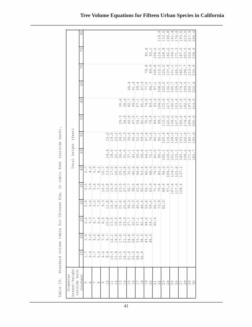
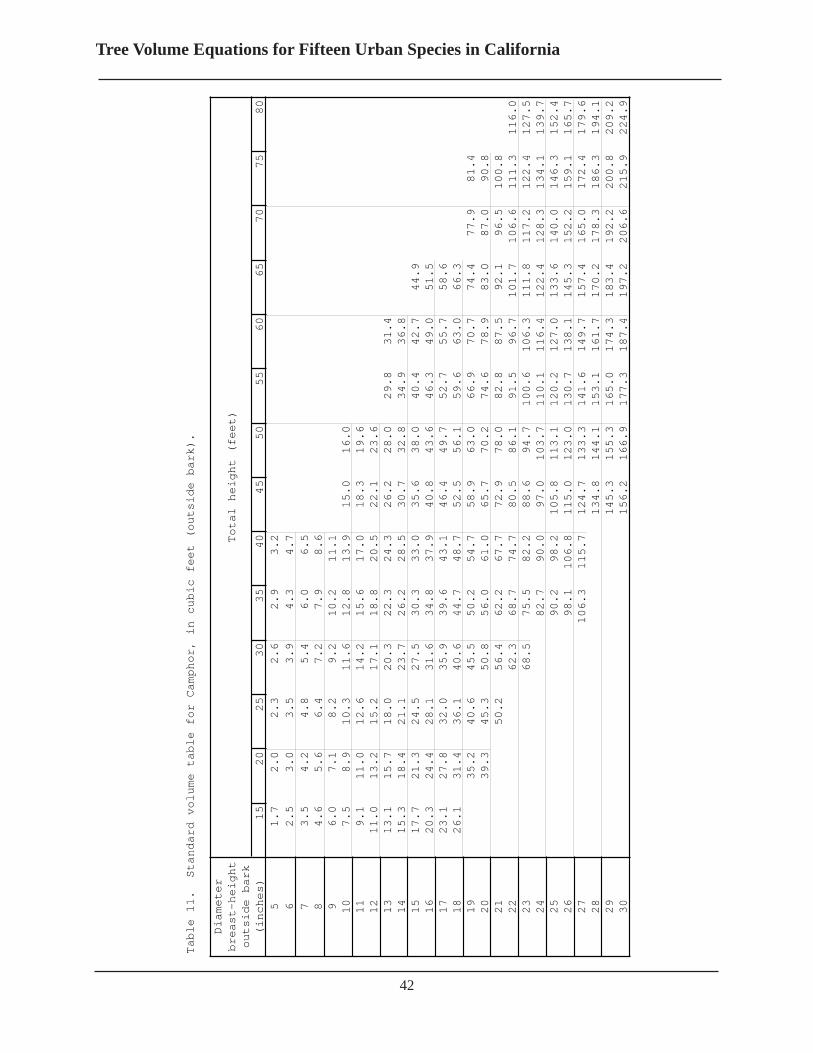
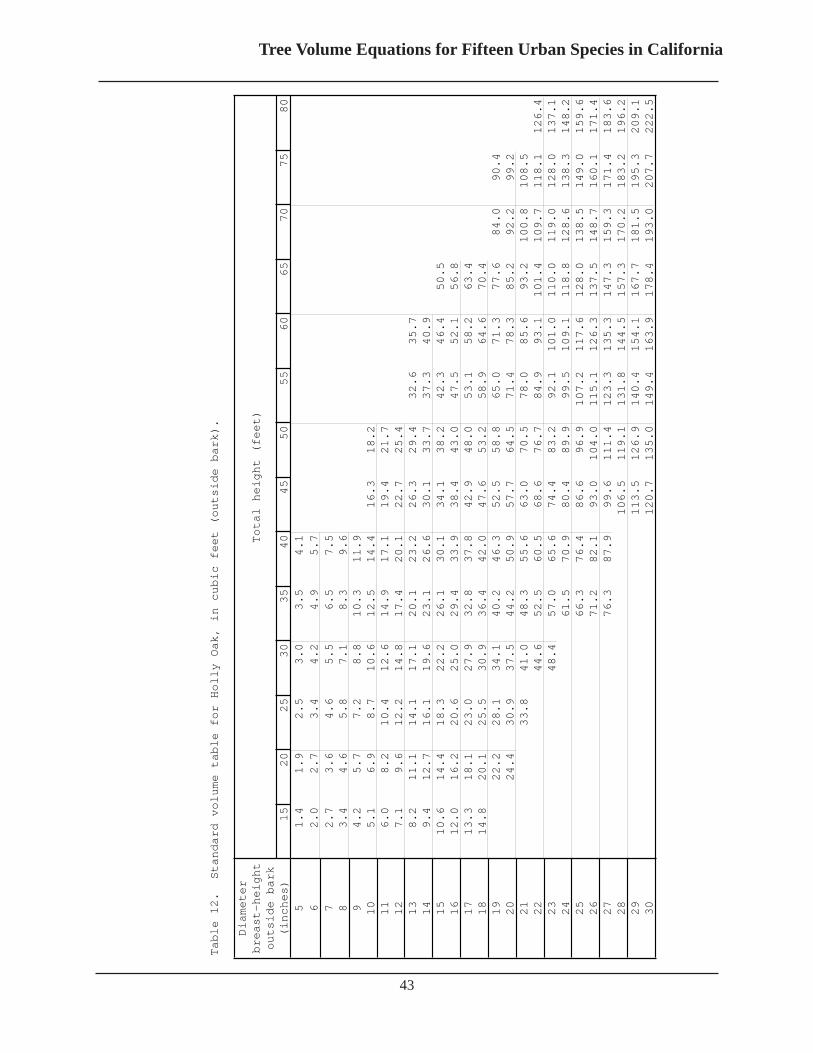
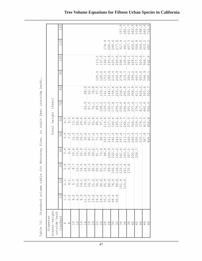
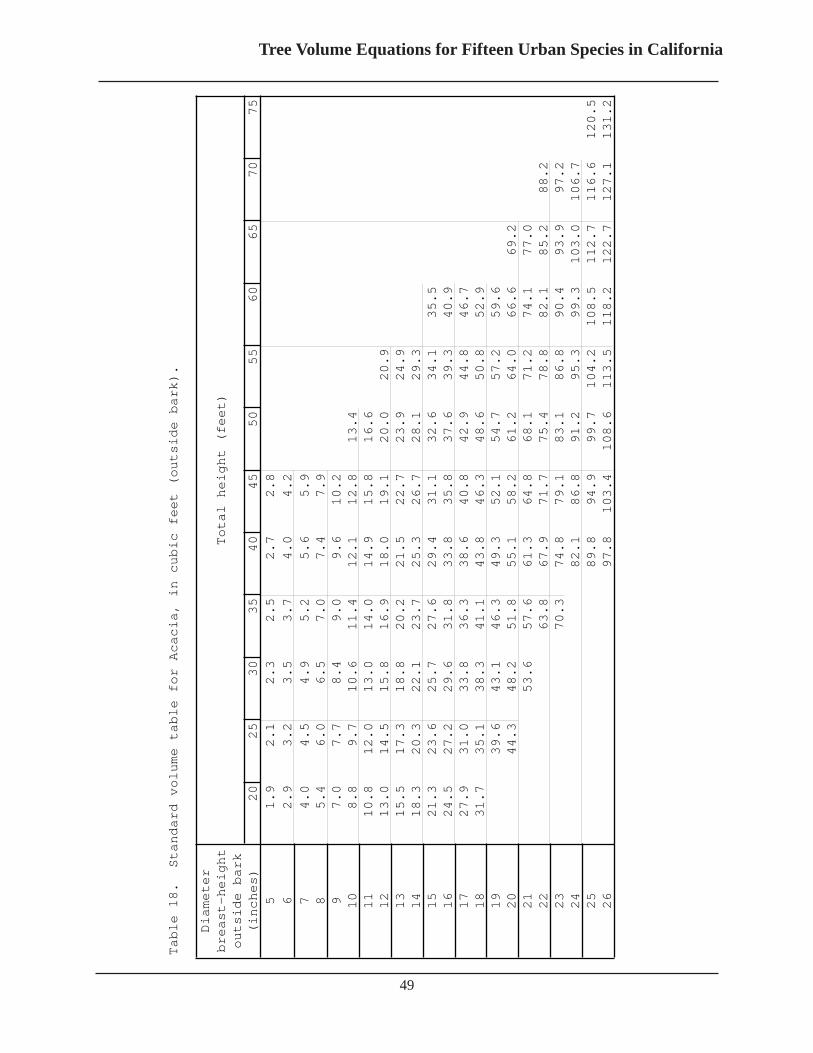
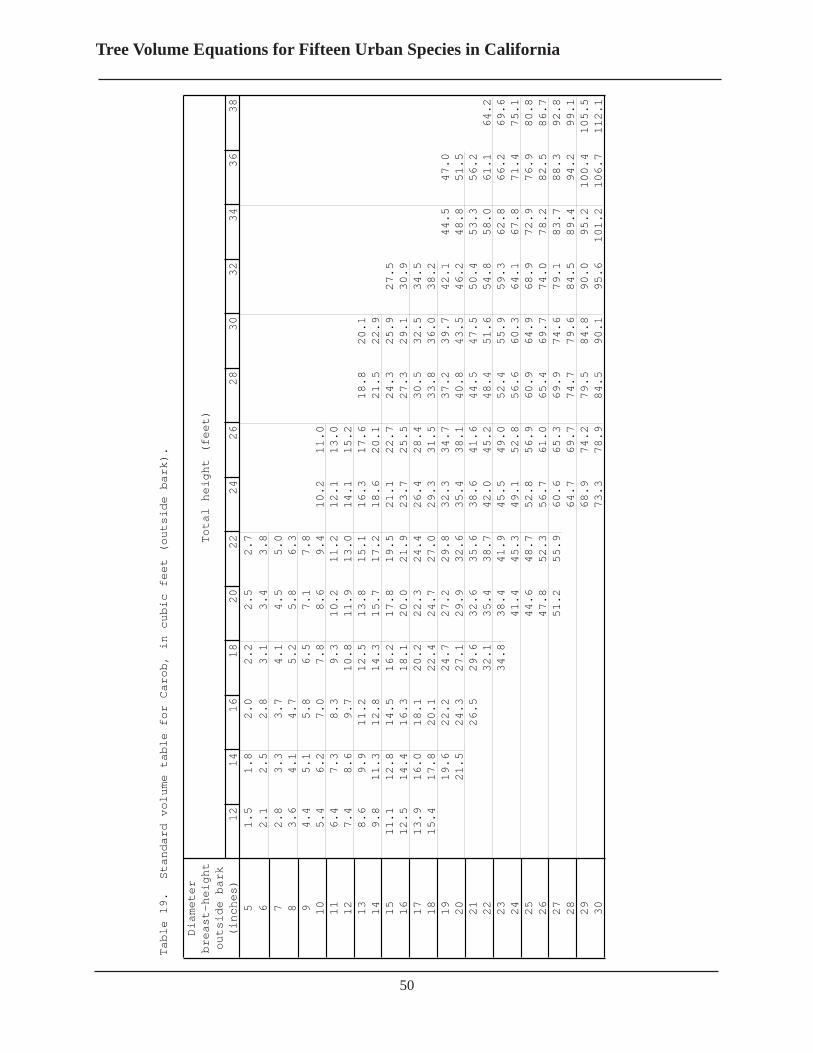
Use of Volume Tables. Volume tables arebest used when the volume of only a few treesis needed. The volume tables in the Appendixare arranged in diameter classes of 1” andheight classes of 5’. Two options are possible,depending on your need. Diameter and heightdata can either be rounded to the nearest inch,and nearest 5’ respectively to obtain a roughvolume estimate, or, you will need to doubleinterpolate the table to eliminate roundingerror (see “Calculating tree volume from avolume table by the rounding, and the doubleinterpolation method” in the Appendix.).

Regardless of the method used, theprocess is repeated for each tree until finished.Next volume estimates are summed byspecies, and again for all species. Theproportion of volume by segment diametercan be estimated from Figure 11.

32

Tree Volume Equations for Fifteen Urban Species in California

33

Tree Volume Equations for Fifteen Urban Species in California

IX. Summary and Conclusions

As communities strive for sustainability of their urban forestry programs, increasedattention must be paid to the wood resource of the urban forest. To manage for these values,comprehensive inventories and databases are needed. A new level of sophistication andcommitment is necessary to build these inventories and to make use of them to further theprogram’s goals.

The urban forester must be capable of properly measuring specific characteristics of a treesuch as diameter, height and age in order to use them in calculating the typical managerialmeasures (e.g., basal area, volume and growth rates). These measures can then be combinedwith other quantitative and qualitative measures such as species, location, health and vigorrating, expected life and past treatments to establish a database which will form the foundationfor wood marketing, policymaking and public relations activities.

Practicing urban foresters may have already had education and training in forest inventoryas part of their bachelor’s degree. However, the nuances of measuring native and exotic speciesin open-grown settings influenced by urbanization requires special knowledge and training thatis not typical of most forest measurement and inventory coursework . To acquire the field andanalytical skills needed for this work the urban forester may need to continue their educationthrough shortcourses, workshops, field demonstrations and educational videos similar to the onepresented at the Symposium on Oak Woodlands: Ecology, Management and Urban InterfaceIssues (Pillsbury and Reimer 1996). These continuing education experiences will also facilitatebetter networking between practicing urban foresters on a broad range of issues, concerns andpotential solutions.

Although considerable resources must be committed to designing and maintaining thesecomprehensive urban forest inventories, long-term benefits including a healthy urban forest thatis both biologically and economically sound, will more than justify the expense throughimproved forest management, regularized maintenance, and new funding sources. It is thesetypes of outcomes that the urban forester can point to as evidence of sustainable management.

34

Tree Volume Equations for Fifteen Urban Species in California

De Lasaux, M. J. and N. H. Pillsbury. 1990.Young-Growth Sierra Redwood VolumeEquations for Mountain HomeDemonstration State Forest, CaliforniaDepartment of Forestry and FireProtection, Sacramento, CA. NaturalResources Management Department, CalPoly State University, San Luis Obispo,CA. 12 p.

Draper, N. R. and H. Smith. 1981. AppliedRegression Analysis. Second edition. JohnWiley and Sons. New York. 709 p.

Husch, B., C. Miller and T. Beers. 1982.Forest Mensuration. Third Edition. JohnWiley and Sons, New York. 402 p.

Larson, T. and T. O’Keefe. 1996. GreenwasteReduction Implementation Plan (GRIP), anUrban Forestry Biomass UtilizationProject. Intregrated Urban Forestry, Inc.,Laguna Hills, and Cal Poly, San LuisObispo. 5 p.

Pillsbury, N. H. 1994. Aspen Inventory,Assessment, and Management on the KernPlateau, Sequoia National Forest. (USDA-Forest Service, Porterville, CA.) NaturalResources Management Dept., Cal PolyState Univ., San Luis Obispo, California.551 p.

Pillsbury, N. H. and D. R. Hermosilla. 1993.Biomass Farm Demonstration Project;1992 Measurements. CaliforniaDepartment of Forestry and FireProtection, Sacramento, CA. NaturalResources Management Dept., Cal PolyState Univ., San Luis Obispo, California.230 p.

X. Literature Cited

Pillsbury, N. H. and M. L. Kirkley. 1984.Equations for Total, Wood, and Saw-LogVolume for Thirteen CaliforniaHardwoods. Research Note PNW-414.Portland, OR: U.S. Department ofAgriculture, Forest Service, PacificNorthwest Forest and Range ExperimentStation. 52 p.

Pillsbury, N., P. McDonald and V. Simon.1995. Reliability of Tanoak VolumeEquations When Applied To DifferentAreas. Western Journal of AppliedForestry 10(2). pp. 1-7.

Pillsbury, N. H. and R. D. Pryor. 1989.Volume Equations for Young GrowthSoftwood and Hardwood Species at BoggsMountain Demonstration State Forest,California Department of Forestry and FireProtection, Sacramento, CA. NaturalResources Management Dept., Cal PolyState Univ., San Luis Obispo, California.100 p.

Pillsbury, N. H. and R. D. Pryor. 1992.Volume Equations for Young GrowthSoftwood and Hardwood Species at BoggsMountain Demonstration State Forest.California State Forest Note. CaliforniaDepartment of Forestry and FireProtection, Sacramento, CA. 8 p.

Pillsbury, N. H. and R. D. Pryor. 1994.Volume Equations for Canyon Live Oak inthe San Bernardino Mountains of SouthernCalifornia. West. J. Appl. Forestry 9 (2):46-51.

35

Tree Volume Equations for Fifteen Urban Species in California

Pillsbury, N. H., J. L. Reimer and R.Thompson. 1996. Cal Poly Urban ForestSustainability Project. A 22 minute digitalvideo presented at the Symposium on OakWoodlands: Ecology, Management, andUrban Interface Issues, March 19-22, 1996,Cal Poly, San Luis Obispo, CA.

Pillsbury, N. H. and J. L. Reimer. 1997. TreeVolume Equations for 10 Urban Species inCalifornia in Proceedings of a Symposiumon Oak Woodlands: Ecology, Management,and Urban Interface Issues (TechnicalCoordinators: Pillsbury, N. H., J. Vernerand W. D. Tietje); 19-22 March 1996; SanLuis Obispo, CA. Gen. Tech. Rep. PSW-GTR-160. Albany, CA: Pacific SouthwestResearch Station, Forest Service, U.S.Department of Agriculture; 738 p.

Pillsbury, N. H. and R. Thompson. 1995.Tree Volume Equations for Fifteen UrbanSpecies in California. Interim Report.Urban Forest Ecosystems Institute, CalPoly, San Luis Obispo, and CaliforniaDepartment of Forestry and FireProtection, Riverside. 45 p.

Pillsbury, N. H., R. Standiford, L. Costello, T.Rhoades, and P. Regan (Banducci). 1989.Wood Volume Equations for Central CoastBlue Gum (Eucalyptus globulus).Published in California Agriculture,Volume 43, Number 6. University ofCalifornia.

Snedecor, George W. and William G.Cochran. 1967. Statistical Methods. Sixthedition. The Iowa State University Press.Ames. 593 p.

Thompson, R., N. Pillsbury and J. Hanna.1994. The Elements of Sustainability inUrban Forestry. Tech. Rept. No. 1. UrbanForest Ecosystems Institute, Cal Poly StateUniversity, San Luis Obispo. 56 p.

36

Tree Volume Equations for Fifteen Urban Species in California

37

Tree Volume Equations for Fifteen Urban Species in California

X. Appendix

38

Tree Volume Equations for Fifteen Urban Species in California

39

Tree Volume Equations for Fifteen Urban Species in California

1. Rounding diameter and height to the nearest class

Using rounded values gives a diameter of 17” and a height of 55’. Intersecting thevolume table gives a cubic foot value of 55.

2. Double interpolating to obtain volume

a) The first step is to interpolate the volume of a 16.8” diameter tree for heights of 50’and 55’. The ratio for each is shown below.

Calculating treevolume from avolume table by therounding, and thedouble interpolationmethod.

Table 10. Standard volume table for Chinese Elm, in cubic feet.

Diameterbreast-height Total height (feet)outside bark

(inches) 15 20 25 30 35 40 45 50 55 605 2 2 2 2 3 36 3 3 3 4 4 47 4 4 5 5 6 68 5 6 6 7 8 89 7 8 8 9 10 1110 8 10 11 12 13 14 14 1511 10 12 13 15 16 17 18 1912 13 15 17 18 19 21 22 2313 15 18 20 22 23 25 27 28 29 3114 18 21 24 26 28 30 32 33 35 3615 22 25 28 30 33 35 37 39 41 4316 25 29 32 35 38 41 43 45 48 5017 29 33 37 41 44 47 50 52 55 5718 33 38 42 46 50 53 57 60 63 65

Example is for aChinese elm 16.8” indbh, and 54.2’ in ht.

Note: For simplicity,values in the volume tableshown above are roundedto the nearest integer.

x

3.0=

4.25.0

x = 2.52. 50.6 + 2.52 = 53.1 cf

b) The last step is to interpolate the volume for a 54.2’ tree, by the following ratio.Note the answer is close to the equation result, but a lot more work.

For 50' , 16.8" tree: 0.81.0

=x

7 x = 5.6, 45.0 + 5.6 = 50.6 cf

For 55' , 16.8" tree: 0.8

1.0=

x

7 x = 5.6, 48.0 + 5.6 = 53.6 cf

50 ft 54.2 ft 55 ft

50.6 cf 53.1 cf 53.6 cf

4.2

x

5.0

3.0

Total HeightDbh 50.00 55.00

16.00 45.00 48.00

16.80 50.60 53.60

17.00 52.00 55.00

1.00.8 x

7.0 7.0

x

40

Tree Volume Equations for Fifteen Urban Species in California

Table 9. Local volume tables for selected urban forest species, in cubic feet (outside bark).

DBH

Southland

Species

Coastal

Species

Central Valley Species

DBH

outside

outside

bark

Monterey

Monterey

Chinese

London

Modesto

Sawleaf

Southern

bark

(inches)

Camphor

Chinese Elm

Holly Oak

Jacaranda

Liquidambar

Blue Gum

Pine

Cypress

Acacia

Carob

Pistache

Plane

Ash

Zelkova

Magnolia

(inches)

51.9

2.0

1.7

2.0

1.9

2.8

1.5

2.0

2.1

2.0

1.7

1.9

1.5

1.6

1.5

56

3.0

3.2

2.7

3.1

3.0

4.3

2.4

3.1

3.3

3.0

2.9

3.0

2.5

2.6

2.5

67

4.4

4.9

4.0

4.6

4.5

6.3

3.6

4.6

4.7

4.2

4.5

4.6

3.7

3.9

3.7

78

6.1

6.9

5.7

6.4

6.3

8.8

5.1

6.4

6.4

5.5

6.5

6.5

5.3

5.6

5.3

89

8.2

9.4

7.7

8.5

8.5

11.7

7.0

8.6

8.4

7.1

9.1

9.0

7.2

7.7

7.2

910

10.8

12.4

10.2

11.1

11.2

15.1

9.2

11.1

10.8

8.9

12.2

11.9

9.6

10.2

9.5

10

11

13.7

16.0

13.1

14.0

14.2

19.0

11.9

14.1

13.5

10.9

16.0

15.3

12.3

13.1

12.2

11

12

17.1

20.1

16.4

17.4

17.8

23.5

15.0

17.5

16.5

13.1

20.4

19.3

15.4

16.5

15.4

12

13

20.9

24.9

20.2

21.3

21.8

28.6

18.5

21.4

20.0

15.6

25.6

23.9

19.1

20.5

19.0

13

14

25.3

30.2

24.5

25.6

26.4

34.2

22.6

25.8

23.8

18.2

31.5

29.2

23.2

25.0

23.0

14

15

30.1

36.3

29.3

30.3

31.5

40.5

27.2

30.6

27.9

21.1

38.2

35.1

27.8

30.0

27.6

15

16

35.5

43.0

34.7

35.6

37.2

47.4

32.3

36.0

32.5

24.2

45.8

41.7

33.0

35.7

32.7

16

17

41.3

50.5

40.6

41.4

43.4

54.9

37.9

41.9

37.5

27.6

54.3

49.0

38.7

42.0

38.3

17

18

47.8

58.7

47.2

47.8

50.2

63.1

44.2

48.3

42.9

31.2

63.7

57.1

44.9

48.9

44.5

18

19

54.8

67.7

54.3

54.6

57.7

72.0

51.0

55.2

48.7

35.0

74.2

66.0

51.8

56.5

51.3

19

20

62.4

77.5

62.1

62.1

65.8

81.6

58.5

62.8

54.9

39.0

85.7

75.7

59.3

64.8

58.6

20

21

70.6

88.1

70.5

70.1

74.5

91.9

66.6

70.9

61.6

43.3

98.3

86.3

67.4

73.9

66.6

21

22

79.5

99.6

79.6

78.6

84.0

103.0

75.4

79.6

68.7

47.8

112.0

97.7

76.2

83.7

75.3

22

23

88.9

112.0

89.4

87.8

94.1

114.7

84.9

89.0

76.2

52.5

126.9

110.0

85.7

94.2

84.6

23

24

99.1

125.4

99.9

97.6

104.9

127.3

95.1

98.9

84.2

57.5

143.0

123.3

95.9

105.6

94.6

24

25

109.9

139.6

108.1

116.5

140.6

106.0

109.6

92.7

62.7

160.4

137.5

106.7

117.8

105.3

25

26

121.4

154.8

119.1

154.7

117.7

120.8

101.6

68.2

179.0

152.7

118.3

130.8

116.7

26

27

133.5

171.1

169.6

130.1

132.8

73.9

199.1

168.9

130.7

144.7

128.8

27

28

146.4

185.3

143.4

145.4

79.8

220.5

186.2

143.9

159.5

141.7

28

29

160.1

201.9

157.5

158.7

86.0

243.3

204.5

157.8

175.2

155.3

29

30

174.4

219.3

172.3

172.7

92.4

267.6

223.9

172.5

191.8

169.8

30

31

237.5

188.1

187.4

188.1

209.4

185.0

31

32

256.6

204.7

202.8

204.5

227.9

201.1

32

33

276.6

222.2

219.0

221.7

247.5

218.0

33

34

297.5

240.6

236.0

239.9

268.0

235.7

34

35

319.2

260.0

253.7

258.9

289.7

254.4

35

36

341.9

280.2

272.2

278.8

312.3

273.9

36

37

365.5

301.5

291.4

299.7

336.1

294.3

37

38

390.1

323.7

311.5

321.5

360.9

315.6

38

39

415.6

346.9

332.3

344.3

386.9

337.8

39

40

442.0

371.1

354.0

368.0

414.0

361.0

40

41

469.4

396.4

376.5

41

42

497.8

422.7

399.8

42

43

527.2

450.0

424.0

43

44

557.6

478.5

449.0

44

45

589.0

508.0

474.9

45

46

621.4

501.7

46

47

654.8

529.4

47

48

689.3

557.9

48

49

724.8

587.4

49

50

761.4

617.7

50

51

799.0

649.0

51

52

837.7

681.2

52

53

877.5

714.4

53

54

918.4

748.5

54

55

960.4

783.6

55

56

819.6

56

57

856.6

57

58

894.6

58

59

933.6

59

60

973.6

60

41

Tree Volume Equations for Fifteen Urban Species in California

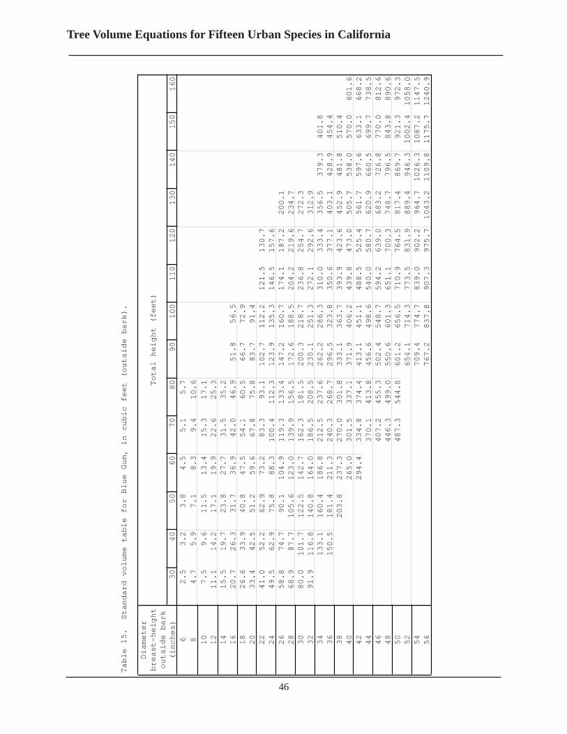
Table 10. Standard volume table for Chinese Elm, in cubic feet (outside bark).

Diameter

breast-height

Total height (feet)

outside bark

(inches)

15

20

25

30

35

40

45

50

55

60

65

70

75

80

51.7

1.9

2.2

2.4

2.5

2.7

62.6

3.0

3.3

3.6

3.9

4.2

73.7

4.2

4.7

5.2

5.6

5.9

85.0

5.8

6.4

7.0

7.6

8.1

96.6

7.6

8.5

9.3

10.0

10.7

10

8.4

9.7

10.8

11.8

12.8

13.6

14.4

15.2

11

10.5

12.1

13.5

14.8

15.9

17.0

18.0

19.0

12

12.8

14.8

16.5

18.1

19.5

20.8

22.1

23.2

13

15.5

17.8

19.9

21.8

23.5

25.1

26.6

28.0

29.3

30.6

14

18.4

21.2

23.6

25.8

27.9

29.8

31.6

33.3

34.9

36.4

15

21.6

24.8

27.7

30.3

32.7

35.0

37.1

39.0

40.9

42.7

44.4

16

25.0

28.9

32.2

35.3

38.0

40.6

43.1

45.4

47.5

49.6

51.6

17

28.8

33.2

37.1

40.6

43.8

46.8

49.6

52.2

54.7

57.1

59.4

18

32.9

38.0

42.4

46.4

50.0

53.4

56.6

59.6

62.5

65.3

67.9

19

43.0

48.0

52.6

56.7

60.6

64.2

67.6

70.9

74.0

77.0

79.8

82.6

20

48.5

54.1

59.2

63.9

68.3

72.3

76.2

79.9

83.4

86.7

89.9

93.1

21

60.6

66.3

71.6

76.5

81.0

85.3

89.5

93.4

97.1

100.8

104.2

22

73.9

79.8

85.2

90.3

95.1

99.7

104.0

108.2

112.3

116.1

119.9

23

82.0

88.4

94.5

100.1

105.4

110.5

115.4

120.0

124.5

128.8

133.0

24

97.6

104.3

110.5

116.4

122.0

127.4

132.5

137.4

142.2

146.8

25

107.4

114.7

121.5

128.0

134.2

140.0

145.7

151.1

156.3

161.4

26

117.6

125.6

133.1

140.2

147.0

153.4

159.6

165.5

171.3

176.8

27

128.4

137.1

145.3

153.1

160.4

167.5

174.2

180.7

187.0

193.0

28

158.2

166.6

174.6

182.3

189.6

196.7

203.5

210.0

29

171.6

180.7

189.4

197.8

205.7

213.4

220.8

227.9

30

185.7

195.6

205.0

214.0

222.6

230.9

238.9

246.6

42

Tree Volume Equations for Fifteen Urban Species in California

Table 11. Standard volume table for Camphor, in cubic feet (outside bark).

Diameter

breast-height

Total height (feet)

outside bark

(inches)

15

20

25

30

35

40

45

50

55

60

65

70

75

80

51.7

2.0

2.3

2.6

2.9

3.2

62.5

3.0

3.5

3.9

4.3

4.7

73.5

4.2

4.8

5.4

6.0

6.5

84.6

5.6

6.4

7.2

7.9

8.6

96.0

7.1

8.2

9.2

10.2

11.1

10

7.5

8.9

10.3

11.6

12.8

13.9

15.0

16.0

11

9.1

11.0

12.6

14.2

15.6

17.0

18.3

19.6

12

11.0

13.2

15.2

17.1

18.8

20.5

22.1

23.6

13

13.1

15.7

18.0

20.3

22.3

24.3

26.2

28.0

29.8

31.4

14

15.3

18.4

21.1

23.7

26.2

28.5

30.7

32.8

34.9

36.8

15

17.7

21.3

24.5

27.5

30.3

33.0

35.6

38.0

40.4

42.7

44.9

16

20.3

24.4

28.1

31.6

34.8

37.9

40.8

43.6

46.3

49.0

51.5

17

23.1

27.8

32.0

35.9

39.6

43.1

46.4

49.7

52.7

55.7

58.6

18

26.1

31.4

36.1

40.6

44.7

48.7

52.5

56.1

59.6

63.0

66.3

19

35.2

40.6

45.5

50.2

54.7

58.9

63.0

66.9

70.7

74.4

77.9

81.4

20

39.3

45.3

50.8

56.0

61.0

65.7

70.2

74.6

78.9

83.0

87.0

90.8

21

50.2

56.4

62.2

67.7

72.9

78.0

82.8

87.5

92.1

96.5

100.8

22

62.3

68.7

74.7

80.5

86.1

91.5

96.7

101.7

106.6

111.3

116.0

23

68.5

75.5

82.2

88.6

94.7

100.6

106.3

111.8

117.2

122.4

127.5

24

82.7

90.0

97.0

103.7

110.1

116.4

122.4

128.3

134.1

139.7

25

90.2

98.2

105.8

113.1

120.2

127.0

133.6

140.0

146.3

152.4

26

98.1

106.8

115.0

123.0

130.7

138.1

145.3

152.2

159.1

165.7

27

106.3

115.7

124.7

133.3

141.6

149.7

157.4

165.0

172.4

179.6

28

134.8

144.1

153.1

161.7

170.2

178.3

186.3

194.1

29

145.3

155.3

165.0

174.3

183.4

192.2

200.8

209.2

30

156.2

166.9

177.3

187.4

197.2

206.6

215.9

224.9

43

Tree Volume Equations for Fifteen Urban Species in California

Table 12. Standard volume table for Holly Oak, in cubic feet (outside bark).

Diameter

breast-height

Total height (feet)

outside bark

(inches)

15

20

25

30

35

40

45

50

55

60

65

70

75

80

51.4

1.9

2.5

3.0

3.5

4.1

62.0

2.7

3.4

4.2

4.9

5.7

72.7

3.6

4.6

5.5

6.5

7.5

83.4

4.6

5.8

7.1

8.3

9.6

94.2

5.7

7.2

8.8

10.3

11.9

10

5.1

6.9

8.7

10.6

12.5

14.4

16.3

18.2

11

6.0

8.2

10.4

12.6

14.9

17.1

19.4

21.7

12

7.1

9.6

12.2

14.8

17.4

20.1

22.7

25.4

13

8.2

11.1

14.1

17.1

20.1

23.2

26.3

29.4

32.6

35.7

14

9.4

12.7

16.1

19.6

23.1

26.6

30.1

33.7

37.3

40.9

15

10.6

14.4

18.3

22.2

26.1

30.1

34.1

38.2

42.3

46.4

50.5

16

12.0

16.2

20.6

25.0

29.4

33.9

38.4

43.0

47.5

52.1

56.8

17

13.3

18.1

23.0

27.9

32.8

37.8

42.9

48.0

53.1

58.2

63.4

18

14.8

20.1

25.5

30.9

36.4

42.0

47.6

53.2

58.9

64.6

70.4

19

22.2

28.1

34.1

40.2

46.3

52.5

58.8

65.0

71.3

77.6

84.0

90.4

20

24.4

30.9

37.5

44.2

50.9

57.7

64.5

71.4

78.3

85.2

92.2

99.2

21

33.8

41.0

48.3

55.6

63.0

70.5

78.0

85.6

93.2

100.8

108.5

22

44.6

52.5

60.5

68.6

76.7

84.9

93.1

101.4

109.7

118.1

126.4

23

48.4

57.0

65.6

74.4

83.2

92.1

101.0

110.0

119.0

128.0

137.1

24

61.5

70.9

80.4

89.9

99.5

109.1

118.8

128.6

138.3

148.2

25

66.3

76.4

86.6

96.9

107.2

117.6

128.0

138.5

149.0

159.6

26

71.2

82.1

93.0

104.0

115.1

126.3

137.5

148.7

160.1

171.4

27

76.3

87.9

99.6

111.4

123.3

135.3

147.3

159.3

171.4

183.6

28

106.5

119.1

131.8

144.5

157.3

170.2

183.2

196.2

29

113.5

126.9

140.4

154.1

167.7

181.5

195.3

209.1

30

120.7

135.0

149.4

163.9

178.4

193.0

207.7

222.5

44

Tree Volume Equations for Fifteen Urban Species in California

Table 13. Standard volume table for Jacaranda, in cubic feet (outside bark).

Diameter

breast-height

Total height (feet)

outside bark

(inches)

15

20

25

30

35

40

45

50

55

60

65

70

75

80

51.7

2.0

2.2

2.5

2.7

2.9

62.5

2.9

3.3

3.7

4.0

4.3

73.5

4.1

4.6

5.1

5.6

6.0

84.7

5.5

6.2

6.9

7.5

8.0

96.1

7.1

8.0

8.9

9.7

10.4

10

7.7

9.0

10.1

11.2

12.2

13.1

14.0

14.8

11

9.4

11.0

12.5

13.8

15.0

16.1

17.2

18.2

12

11.4

13.3

15.1

16.7

18.1

19.5

20.8

22.1

13

13.6

15.9

18.0

19.9

21.6

23.2

24.8

26.3

27.7

29.0

14

16.0

18.7

21.1

23.3

25.4

27.3

29.2

30.9

32.5

34.1

15

18.6

21.7

24.6

27.1

29.5

31.8

33.9

35.9

37.8

39.7

41.5

16

21.4

25.0

28.3

31.3

34.0

36.6

39.0

41.4

43.6

45.7

47.8

17

24.4

28.6

32.3

35.7

38.8

41.8

44.6

47.2

49.8

52.2

54.5

18

27.7

32.4

36.6

40.4

44.0

47.3

50.5

53.5

56.4

59.1

61.8

19

36.4

41.2

45.5

49.5

53.3

56.8

60.2

63.4

66.5

69.5

72.4

75.2

20

40.8

46.1

50.9

55.4

59.6

63.6

67.4

71.0

74.4

77.8

81.0

84.1

21

51.3

56.6

61.6

66.3

70.7

74.9

79.0

82.8

86.5

90.1

93.6

22

62.7

68.2

73.4

78.3

83.0

87.4

91.7

95.8

99.8

103.6

107.3

23

69.1

75.2

80.9

86.3

91.4

96.3

101.0

105.6

109.9

114.2

118.3

24

82.5

88.8

94.7

100.3

105.7

110.9

115.9

120.7

125.3

129.8

25

90.2

97.1

103.6

109.7

115.6

121.2

126.7

131.9

137.0

141.9

26

98.3

105.8

112.8

119.5

125.9

132.1

138.0

143.7

149.3

154.7

27

106.8

114.9

122.5

129.8

136.8

143.5

149.9

156.1

162.1

167.9

28

132.7

140.6

148.1

155.3

162.3

169.0

175.5

181.8

29

143.2

151.8

159.9

167.7

175.2

182.5

189.5

196.3

30

154.3

163.4

172.2

180.6

188.7

196.5

204.1

211.4

45

Tree Volume Equations for Fifteen Urban Species in California

Table 14. Standard volume table for Liquidambar, in cubic feet (outside bark).

Diameter

breast-height

Total height (feet)

outside bark

(inches)

15

20

25

30

35

40

45

50

55

60

65

70

75

80

51.5

1.7

1.9

2.0

2.1

2.3

62.3

2.6

2.8

3.1

3.3

3.5

73.3

3.7

4.1

4.4

4.7

4.9

84.5

5.0

5.5

6.0

6.4

6.7

95.9

6.6

7.3

7.8

8.4

8.8

10

7.5

8.5

9.3

10.0

10.7

11.3

11.9

12.4

11

9.4

10.6

11.6

12.5

13.3

14.1

14.8

15.4

12

11.5

12.9

14.2

15.3

16.3

17.2

18.1

18.9

13

13.8

15.5

17.0

18.4

19.6

20.7

21.8

22.7

23.7

24.5

14

16.4

18.4

20.2

21.8

23.3

24.6

25.8

27.0

28.1

29.1

15

19.2

21.6

23.7

25.6

27.3

28.9

30.3

31.7

33.0

34.2

35.3

16

22.3

25.1

27.6

29.7

31.7

33.5

35.2

36.8

38.3

39.7

41.0

17

25.7

28.9

31.7

34.2

36.5

38.6

40.5

42.3

44.0

45.7

47.2

18

29.3

33.0

36.2

39.1

41.7

44.0

46.3

48.3

50.3

52.1

53.9

19

37.4

41.1

44.3

47.2

49.9

52.4

54.8

57.0

59.1

61.1

63.0

64.8

20

42.1

46.2

49.9

53.2

56.2

59.0

61.7

64.2

66.5

68.8

70.9

73.0

21

51.8

55.8

59.5

62.9

66.1

69.1

71.8

74.5

77.0

79.4

81.7

22

62.2

66.3

70.1

73.6

76.9

80.0

83.0

85.8

88.5

91.0

93.5

23

68.9

73.5

77.7

81.6

85.2

88.7

92.0

95.1

98.0

100.9

103.6

24

81.1

85.7

90.0

94.1

97.9

101.5

104.9

108.2

111.3

114.4

25

89.2

94.2

99.0

103.4

107.6

111.5

115.3

118.9

122.4

125.7

26

97.6

103.2

108.4

113.2

117.8

122.2

126.3

130.2

134.0

137.7

27

106.5

112.6

118.3

123.6

128.6

133.3

137.8

142.1

146.3

150.2

28

128.7

134.4

139.9

145.0

149.9

154.6

159.1

163.4

29

139.6

145.8

151.7

157.3

162.6

167.7

172.6

177.3

30

151.0

157.7

164.1

170.1

175.9

181.4

186.7

191.8

46

Tree Volume Equations for Fifteen Urban Species in California

Table 15. Standard volume table for Blue Gum, in cubic feet (outside bark).

Diameter

breast-height

Total height (feet)

outside bark

(inches)

30

40

50

60

70

80

90

100

110

120

130

140

150

160

62.5

3.2

3.8

4.5

5.1

5.7

84.7

5.9

7.1

8.3

9.4

10.6

10

7.5

9.6

11.5

13.4

15.3

17.1

12

11.1

14.2

17.1

19.9

22.6

25.3

14

15.5

19.7

23.8

27.7

31.5

35.2

16

20.7

26.3

31.7

36.9

42.0

46.9

51.8

56.5

18

26.6

33.9

40.8

47.5

54.1

60.5

66.7

72.9

20

33.4

42.5

51.2

59.6

67.8

75.8

83.7

91.4

22

41.0

52.2

62.9

73.2

83.3

93.1

102.7

112.2

121.5

130.7

24

49.5

62.9

75.8

88.3

100.4

112.3

123.9

135.3

146.5

157.6

26

58.8

74.7

90.1

104.9

119.3

133.4

147.2

160.7

174.1

187.2

200.1

28

68.9

87.7

105.6

123.0

139.9

156.5

172.6

188.5

204.2

219.6

234.7

30

80.0

101.7

122.5

142.7

162.3

181.5

200.3

218.7

236.8

254.7

272.3

32

91.9

116.8

140.8

164.0

186.5

208.5

230.1

251.3

272.1

292.6

312.9

34

133.1

160.4

186.8

212.5

237.6

262.2

286.3

310.0

333.4

356.5

379.3

401.8

36

150.5

181.4

211.3

240.3

268.7

296.5

323.8

350.6

377.1

403.1

428.9

454.4

38

203.8

237.3

270.0

301.8

333.1

363.7

393.9

423.6

452.9

481.8

510.4

40

265.0

301.5

337.1

371.9

406.2

439.8

473.0

505.7

538.0

570.0

601.6

42

294.4

334.8

374.4

413.1

451.1

488.5

525.4

561.7

597.6

633.1

668.2

44

370.1

413.8

456.6

498.6

540.0

580.7

620.9

660.5

699.7

738.5

46

407.2

455.3

502.4

548.7

594.2

639.0

683.2

726.8

770.0

812.6

48

446.3

499.0

550.6

601.3

651.1

700.3

748.7

796.5

843.8

890.6

50

487.3

544.8

601.2

656.5

710.9

764.5

817.4

869.7

921.3

972.3

52

654.1

714.3

773.5

831.9

889.4

946.3

1002.4

1058.0

54

709.4

774.7

839.0

902.2

964.7

1026.3

1087.2

1147.5

56

767.2

837.8

907.3

975.7

1043.2

1109.8

1175.7

1240.9

47

Tree Volume Equations for Fifteen Urban Species in California

Table 16. Standard volume table for Monterey Pine, in cubic feet (outside bark).

Diameter

breast-height

Total height (feet)

outside bark

(inches)

10

20

30

40

50

60

70

80

90

100

110

120

61.3

2.1

2.8

3.4

3.9

4.5

82.5

4.1

5.3

6.4

7.5

8.5

10

4.2

6.7

8.7

10.6

12.3

13.9

12

6.3

10.0

13.1

15.9

18.5

20.8

14

8.9

14.1

18.5

22.4

26.0

29.4

16

11.9

19.0

24.9

30.2

35.0

39.6

43.9

48.0

18

15.5

24.7

32.3

39.2

45.5

51.4

57.0

62.3

20

19.6

31.2

40.9

49.6

57.6

65.0

72.1

78.8

22

24.2

38.5

50.6

61.3

71.2

80.4

89.1

97.5

105.4

113.1

24

29.4

46.8

61.4

74.4

86.4

97.6

108.2

118.3

128.0

137.3

26

35.2

55.9

73.3

88.9

103.2

116.6

129.3

141.4

153.0

164.1

174.9

28

41.5

66.0

86.5

104.9

121.7

137.5

152.5

166.7

180.4

193.6

206.3

30

48.4

76.9

100.9

122.3

142.0

160.4

177.8

194.4

210.4

225.7

240.6

32

55.8

88.8

116.5

141.2

163.9

185.2

205.3

224.5

242.9

260.6

277.8

34

101.6

133.3

161.6

187.6

211.9

235.0

256.9

278.0

298.3

317.9

337.0

36

115.4

151.4

183.5

213.1

240.7

266.8

291.8

315.7

338.8

361.1

382.7

38

170.8

207.0

240.3

271.5

301.0

329.1

356.1

382.1

407.3

431.7

40

232.0

269.4

304.3

337.4

368.9

399.2

428.3

456.5

483.9

42

258.7

300.3

339.3

376.1

411.3

445.0

477.5

508.9

539.4

44

333.1

376.3

417.2

456.2

493.6

529.6

564.5

598.3

46

367.8

415.5

460.6

503.6

544.9

584.7

623.2

660.6

48

404.3

456.8

506.4

553.7

599.1

642.8

685.2

726.2

48

Tree Volume Equations for Fifteen Urban Species in California

Table 17. Standard volume table for Monterey Cypress, in cubic feet (outside bark).

Diameter

breast-height

Total height (feet)

outside bark

(inches)

20

30

40

50

60

70

80

90

100

110

120

130

62.2

2.8

3.4

3.9

4.4

4.8

84.2

5.4

6.5

7.5

8.4

9.2

10

6.9

9.0

10.7

12.3

13.9

15.3

12

10.5

13.5

16.2

18.6

20.9

23.1

14

14.8

19.1

23.0

26.4

29.6

32.7

16

20.1

25.9

31.0

35.7

40.1

44.2

48.0

51.7

18

26.2

33.8

40.5

46.6

52.3

57.6

62.7

67.5

20

33.2

42.9

51.4

59.2

66.4

73.1

79.6

85.7

22

41.2

53.2

63.8

73.4

82.3

90.7

98.7

106.3

113.6

120.6

24

50.2

64.8

77.6

89.3

100.2

110.4

120.1

129.4

138.3

146.8

26

60.1

77.6

93.0

107.1

120.1

132.3

144.0

155.1

165.7

176.0

185.9

28

71.1

91.7

110.0

126.6

142.0

156.5

170.2

183.3

195.9

208.0

219.8

30

83.1

107.2

128.5

147.9

166.0

182.9

198.9

214.3

229.0

243.2

256.9

32

96.1

124.1

148.7

171.2

192.0

211.6

230.2

247.9

264.9

281.3

297.2

34

142.3

170.6

196.3

220.2

242.7

264.0

284.3

303.9

322.7

340.8

358.5

36

161.9

194.1

223.4

250.6

276.2

300.4

323.6

345.8

367.2

387.9

407.9

38

219.3

252.4

283.2

312.1

339.5

365.6

390.7

414.9

438.3

460.9

40

283.5

318.0

350.4

381.2

410.6

438.7

465.9

492.1

517.6

42

316.5

355.1

391.3

425.6

458.4

489.9

520.2

549.5

578.0

44

394.4

434.7

472.8

509.3

544.2

577.9

610.5

642.0

46

436.1

480.6

522.8

563.1

601.7

639.0

675.0

709.9

48

480.2

529.1

575.6

619.9

662.5

703.5

743.1

781.6

50

526.6

580.3

631.2

679.9

726.5

771.5

815.0

857.1

52

689.7

742.9

793.9

843.0

890.5

936.6

54

751.2

809.0

864.6

918.1

969.8

1020.0

56

815.5

878.4

938.7

996.8

1052.9

1107.4

58

950.9

1016.1

1079.0

1139.8

1198.8

60

1026.6

1097.1

1165.0

1230.6

1294.3

49

Tree Volume Equations for Fifteen Urban Species in California

Table 18. Standard volume table for Acacia, in cubic feet (outside bark).

Diameter

breast-height

Total height (feet)

outside bark

(inches)

20

25

30

35

40

45

50

55

60

65

70

75

51.9

2.1

2.3

2.5

2.7

2.8

62.9

3.2

3.5

3.7

4.0

4.2

74.0

4.5

4.9

5.2

5.6

5.9

85.4

6.0

6.5

7.0

7.4

7.9

97.0

7.7

8.4

9.0

9.6

10.2

10

8.8

9.7

10.6

11.4

12.1

12.8

13.4

11

10.8

12.0

13.0

14.0

14.9

15.8

16.6

12

13.0

14.5

15.8

16.9

18.0

19.1

20.0

20.9

13

15.5

17.3

18.8

20.2

21.5

22.7

23.9

24.9

14

18.3

20.3

22.1

23.7

25.3

26.7

28.1

29.3

15

21.3

23.6

25.7

27.6

29.4

31.1

32.6

34.1

35.5

16

24.5

27.2

29.6

31.8

33.8

35.8

37.6

39.3

40.9

17

27.9

31.0

33.8

36.3

38.6

40.8

42.9

44.8

46.7

18

31.7

35.1

38.3

41.1

43.8

46.3

48.6

50.8

52.9

19

39.6

43.1

46.3

49.3

52.1

54.7

57.2

59.6

20

44.3

48.2

51.8

55.1

58.2

61.2

64.0

66.6

69.2

21

53.6

57.6

61.3

64.8

68.1

71.2

74.1

77.0

22

63.8

67.9

71.7

75.4

78.8

82.1

85.2

88.2

23

70.3

74.8

79.1

83.1

86.8

90.4

93.9

97.2

24

82.1

86.8

91.2

95.3

99.3

103.0

106.7

25

89.8

94.9

99.7

104.2

108.5

112.7

116.6

120.5

26

97.8

103.4

108.6

113.5

118.2

122.7

127.1

131.2

50

Tree Volume Equations for Fifteen Urban Species in California

Table 19. Standard volume table for Carob, in cubic feet (outside bark).

Diameter

breast-height

Total height (feet)

outside bark

(inches)

12

14

16

18

20

22

24

26

28

30

32

34

36

38

51.5

1.8

2.0

2.2

2.5

2.7

62.1

2.5

2.8

3.1

3.4

3.8

72.8

3.3

3.7

4.1

4.5

5.0

83.6

4.1

4.7

5.2

5.8

6.3

94.4

5.1

5.8

6.5

7.1

7.8

10

5.4

6.2

7.0

7.8

8.6

9.4

10.2

11.0

11

6.4

7.3

8.3

9.3

10.2

11.2

12.1

13.0

12

7.4

8.6

9.7

10.8

11.9

13.0

14.1

15.2

13

8.6

9.9

11.2

12.5

13.8

15.1

16.3

17.6

18.8

20.1

14

9.8

11.3

12.8

14.3

15.7

17.2

18.6

20.1

21.5

22.9

15

11.1

12.8

14.5

16.2

17.8

19.5

21.1

22.7

24.3

25.9

27.5

16

12.5

14.4

16.3

18.1

20.0

21.9

23.7

25.5

27.3

29.1

30.9

17

13.9

16.0

18.1

20.2

22.3

24.4

26.4

28.4

30.5

32.5

34.5

18

15.4

17.8

20.1

22.4

24.7

27.0

29.3

31.5

33.8

36.0

38.2

19

19.6

22.2

24.7

27.2

29.8

32.3

34.7

37.2

39.7

42.1

44.5

47.0

20

21.5

24.3

27.1

29.9

32.6

35.4

38.1

40.8

43.5

46.2

48.8

51.5

21

26.5

29.6

32.6

35.6

38.6

41.6

44.5

47.5

50.4

53.3

56.2

22

32.1

35.4

38.7

42.0

45.2

48.4

51.6

54.8

58.0

61.1

64.2

23

34.8

38.4

41.9

45.5

49.0

52.4

55.9

59.3

62.8

66.2

69.6

24

41.4

45.3

49.1

52.8

56.6

60.3

64.1

67.8

71.4

75.1

25

44.6

48.7

52.8

56.9

60.9

64.9

68.9

72.9

76.9

80.8

26

47.8

52.3

56.7

61.0

65.4

69.7

74.0

78.2

82.5

86.7

27

51.2

55.9

60.6

65.3

69.9

74.6

79.1

83.7

88.3

92.8

28

64.7

69.7

74.7

79.6

84.5

89.4

94.2

99.1

29

68.9

74.2

79.5

84.8

90.0

95.2

100.4

105.5

30

73.3

78.9

84.5

90.1

95.6

101.2

106.7

112.1

51

Tree Volume Equations for Fifteen Urban Species in California

Table 20. Standard volume table for Chinese Pistache in cubic feet (outside bark).

Diameter

breast-height

Total height (feet)

outside bark

(inches)

10

15

20

25

30

35

40

45

50

55

60

65

50.9

1.3

1.7

2.1

2.5

2.8

61.3

1.9

2.5

3.1

3.7

4.2

71.8

2.7

3.5

4.3

5.1

6.0

82.4

3.6

4.7

5.8

6.9

8.0

93.2

4.6

6.1

7.5

8.9

10.3

10

4.0

5.8

7.7

9.5

11.2

13.0

14.8

16.5

11

4.9

7.2

9.5

11.7

13.9

16.0

18.2

20.3

12

5.9

8.7

11.4

14.1

16.8

19.4

22.0

24.6

13

7.1

10.4

13.6

16.8

20.0

23.1

26.2

29.3

32.4

35.4

14

8.3

12.2

16.0

19.8

23.5

27.2

30.8

34.5

38.1

41.7

15

9.7

14.2

18.7

23.0

27.4

31.6

35.9

40.1

44.3

48.5

52.6

16

11.2

16.4

21.5

26.5

31.5

36.4

41.3

46.2

51.0

55.8

60.6

17

12.8

18.7

24.5

30.3

36.0

41.6

47.2

52.8

58.3

63.8

69.2

18

14.5

21.2

27.8

34.3

40.8

47.2

53.5

59.8

66.0

72.3

78.4

19

23.9

31.3

38.7

45.9

53.1

60.2

67.3

74.4

81.4

88.3

95.2

20

26.7

35.0

43.3

51.4

59.4

67.4

75.3

83.2

91.0

98.8

106.6

21

39.0

48.1

57.2

66.1

75.0

83.8

92.6

101.3

110.0

118.6

22

53.3

63.3

73.2

83.1

92.8

102.5

112.2

121.8

131.3

23

58.8

69.8

80.7

91.6

102.3

113.0

123.7

134.2

144.8

24

76.6

88.6

100.5

112.3

124.1

135.7

147.4

158.9

25

83.8

96.9

109.9

122.8

135.7

148.5

161.2

173.8

26

91.3

105.6

119.8

133.9

147.9

161.8

175.6

189.4

27

99.2

114.7

130.1

145.4

160.6

175.7

190.8

205.7

28

140.9

157.5

173.9

190.3

206.6

222.8

29

152.2

170.1

187.8

205.5

223.1

240.6

30

163.9

183.2

202.3

221.4

240.3

259.2

52

Tree Volume Equations for Fifteen Urban Species in California

Table 21. Standard volume table for London Plane, in cubic feet (outside bark).

Diameter

breast-height

Total height (feet)

outside bark

(inches)

10

20

30

40

50

60

70

80

90

100

110

120

62.0

2.7

3.1

3.5

3.8

4.1

84.1

5.3

6.3

7.0

7.7

8.2

10

7.0

9.2

10.8

12.1

13.2

14.2

12

10.9

14.4

16.8

18.8

20.6

22.1

14

15.9

20.9

24.5

27.4

29.9

32.1

16

22.1

28.9

33.9

38.0

41.4

44.5

47.3

49.8

18

29.4

38.6

45.2

50.6

55.2

59.3

63.0

66.4

20

38.0

49.8

58.4

65.4

71.3

76.6

81.4

85.8

22

47.9

62.9

73.7

82.5

90.0

96.7

102.7

108.2

113.3

118.1

24

59.2

77.7

91.1

101.9

111.2

119.5

126.9

133.7

140.0

145.9

26

72.0

94.4

110.7

123.9

135.2

145.2

154.3

162.5

170.2

177.4

184.1

28

86.2

113.1

132.6

148.4

162.0

173.9

184.8

194.7

203.9

212.5

220.6

30

102.0

133.8

156.9

175.6

191.6

205.8

218.6

230.3

241.2

251.4

260.9

32

119.4

156.6

183.6

205.5

224.2

240.8

255.8

269.6

282.3

294.2

305.4

34

181.5

212.8

238.2

259.9

279.2

296.5

312.5

327.2

341.0

354.0

366.2

36

208.7

244.6

273.8

298.8

320.9

340.9

359.2

376.1

392.0

406.9

421.0

38

279.0

312.3

340.8

366.1

388.8

409.7

429.1

447.1

464.1

480.2

40

353.9

386.2

414.8

440.6

464.3

486.2

506.7

525.9

544.2

53

Tree Volume Equations for Fifteen Urban Species in California

Table 22. Standard volume table for Modesto Ash, in cubic feet (outside bark).

Diameter

breast-height

Total height (feet)

outside bark

(inches)

10

20

30

40

50

60

70

80

90

100

60.8

2.2

3.9

5.9

8.1

10.5

81.3

3.6

6.5

9.7

13.4

17.4

10

2.0

5.4

9.6

14.4

19.9

25.8

12

2.8

7.4

13.2

19.9

27.4

35.6

14

3.6

9.7

17.3

26.1

36.0

46.7

16

4.6

12.3

21.9

33.1

45.5

59.0

73.6

89.0

18

5.6

15.1

27.0

40.7

56.0

72.7

90.5

109.6

20

6.8

18.2

32.5

49.0

67.4

87.5

109.0

131.9

22

8.0

21.6

38.5

58.0

79.8

103.5

129.0

156.1

184.7

214.6

24

9.3

25.1

44.8

67.6

93.0

120.7

150.4

181.9

215.3

250.2

26

10.8

28.9

51.6

77.9

107.1

138.9

173.2

209.5

247.9

288.1

28

12.3

33.0

58.9

88.7

122.0

158.3

197.3

238.8

282.5

328.4

30

13.8

37.3

66.5

100.2

137.8

178.8

222.8

269.6

319.0

370.8

32

15.5

41.7

74.5

112.3

154.4

200.4

249.7

302.1

357.5

415.5

34

46.5

82.9

125.0

171.9

223.0

277.9

336.2

397.8

462.4

36

51.4

91.7

138.2

190.1

246.6

307.3

371.9

440.0

511.4

38

100.8

152.0

209.1

271.3

338.1

409.1

484.0

562.5

40

166.4

228.9

296.9

370.0

447.8

529.8

615.8

54

Tree Volume Equations for Fifteen Urban Species in California

Table 23. Standard volume table for Sawleaf Zelkova, in cubic feet (outside bark).

Diameter

breast-height

Total height (feet)

outside bark

(inches)

10

20

30

40

50

60

70

80

90

100

61.6

2.4

3.0

3.5

4.0

4.4

83.2

4.7

5.9

7.0

7.9

8.7

10

5.5

8.0

10.0

11.8

13.3

14.7

12

8.4

12.4

15.5

18.1

20.5

22.7

14

12.1

17.8

22.3

26.1

29.5

32.6

16

16.6

24.4

30.5

35.8

40.5

44.7

48.7

52.4

18

22.0

32.2

40.3

47.2

53.4

59.1

64.3

69.3

20

28.2

41.3

51.7

60.6

68.5

75.8

82.5

88.8

22

35.3

51.8

64.8

75.9

85.9

94.9

103.4

111.3

118.8

125.9

24

43.4

63.6

79.5

93.2

105.5

116.6

127.0

136.7

145.9

154.6

26

52.4

76.8

96.1

112.6

127.4

140.9

153.4

165.1

176.2

186.8

28

62.4

91.5

114.5

134.2

151.8

167.9

182.8

196.8

210.0

222.5

30

73.5

107.8

134.8

158.0

178.7

197.6

215.1

231.6

247.2

261.9

32

85.6

125.5

157.0

184.0

208.1

230.2

250.6

269.8

287.9

305.1

34

144.8

181.2

212.3

240.2

265.6

289.2

311.3

332.2

352.1

36

165.8

207.4

243.1

274.9

304.0

331.0

356.3

380.3

403.0

38

235.6

276.2

312.4

345.5

376.1

404.9

432.1

458.0

40

311.8

352.6

390.0

424.6

457.1

487.8

517.0

55

Tree Volume Equations for Fifteen Urban Species in California

Table 24. Standard volume table for Southern Magnolia, in cubic feet (outside bark).

Diameter

breast-height

Total height (feet)

outside bark

(inches)

10

20

30

40

50

60

70

80

90

100

61.3

2.3

3.3

4.1

5.0

5.8

82.3

4.2

5.9

7.5

9.1

10.6

10

3.7

6.6

9.4

11.9

14.4

16.8

12

5.4

9.7

13.7

17.4

21.0

24.5

14

7.4

13.3

18.8

24.0

28.9

33.8

16

9.8

17.6

24.8

31.6

38.2

44.5

50.7

56.8

18

12.5

22.4

31.6

40.3

48.7

56.8

64.7

72.5

20

15.5

27.9

39.3

50.2

60.6

70.7

80.5

90.1

22

18.9

34.0

47.9

61.1

73.8

86.1

98.1

109.8

121.3

132.6

24

22.7

40.7

57.4

73.2

88.3

103.1

117.4

131.5

145.2

158.8

26

26.7

48.0

67.7

86.3

104.3

121.6

138.6

155.2

171.4

187.4

28

31.2

56.0

78.9

100.7

121.6

141.8

161.6

180.9

199.8

218.4

30

36.0

64.6

91.0

116.1

140.2

163.6

186.4

208.7

230.5

252.0

32

41.1

73.8

104.1

132.7

160.3

187.0

213.0

238.5

263.5

288.0

34

83.7

118.0

150.5

181.7

212.0

241.5

270.4

298.7

326.5

36

94.2

132.8

169.4

204.5

238.6

271.8

304.3

336.2

367.5

38

148.5

189.4

228.8

266.9

304.0

340.4

376.0

411.1

40

210.6

254.4

296.8

338.1

378.5

418.2

457.1

56

Tree Volume Equations for Fifteen Urban Species in California

Space for Notes

57

Tree Volume Equations for Fifteen Urban Species in California

Inside back cover

58

Tree Volume Equations for Fifteen Urban Species in California

Richard A. WilsonDirector

California Department of Forestry and Fire Protection

Douglas P. WheelerSecretary for ResourcesThe Resources Agency

Pete WilsonGovernor

State of California

and FIRE PROTECTIONDEPARTMENT OF FORESTRY

CALIFORNIA

CD

F

FORESTRY

FIRE

Printed on RecycledPaper