Trend Inflation, Indexation, and InflationPersistence in the New Keynesian Phillips Curve∗

Timothy CogleyUniversity of California, Davis

Argia M. SbordoneFederal Reserve Bank of New York

Abstract

A number of empirical studies conclude that purely forward-looking versions

of the New Keynesian Phillips curve (NKPC ) generate too little inflation per-

sistence. Some authors add ad hoc backward-looking terms to address this

shortcoming. In this paper, we hypothesize that inflation persistence results

mainly from variation in the long-run trend component of inflation, attributable

to shifts in monetary policy, and that the apparent need for lagged inflation

in the NKPC comes from neglecting the interaction between drift in trend in-

flation and non-linearities in a more exact version of the model. We derive

a version of the NKPC as a log-linear approximation around a time-varying

inflation trend and examine whether such a model explains the dynamics of in-

flation around that trend. When drift in trend inflation is taken into account,

there is no need for a backward-looking indexation component, and a purely

forward-looking version of the model fits the data well.

JEL Classification: E31. Keywords: Trend inflation; Inflation persistence;

Phillips curve; time-varying VAR.

∗For comments and suggestions, we are grateful to two anonymous referees. We also wish to thankJean Boivin, Mark Gertler, Peter Ireland, Sharon Kozicki, Jim Nason, Luca Sala, Dan Waggoner,Michael Woodford, Tao Zha and seminar participants at the Banque de France, the November2005 NBER Monetary Economics meeting, the October 2005 Conference on Quantitative Models atthe Federal Reserve Bank of Cleveland, the 2004 Society for Computational Economics Meeting inAmsterdam, the Federal Reserve Banks of New York, Richmond, and Kansas City, Duke University,and the Fall 2004 Macro System Committe Meeting in Baltimore. The views expressed in thispaper do not necessarily reflect the position of the Federal Reserve Bank of New York or the FederalReserve System. Please address email to twcogley@ucdavis.edu or argia.sbordone@ny.frb.org.

1

In this paper we consider the extent to which Guillermo Calvo’s (1983) model

of nominal price rigidities can explain inflation dynamics without relying on arbitrary

backward-looking terms. In its baseline formulation, the Calvo model leads to a purely

forward-looking New Keynesian Phillips curve (NKPC): inflation depends on the

expected evolution of real marginal costs. However, purely forward-looking models are

deemed inconsistent with empirical evidence of significant inflation persistence (e.g.,

see Fuhrer and Moore 1995). Accordingly, a number of authors have added backward-

looking elements to enhance the degree of inflation persistence in the model and to

provide a better fit with aggregate data. Lags of inflation are typically introduced

by postulating some form of price indexation (e.g., see Lawrence Christiano, Martin

Eichenbaum and Charles Evans 2005) or rule-of-thumb behavior (e.g., see Jordi Gali

and Mark Gertler 1999). These mechanisms have been criticized because they lack

a convincing microeconomic foundation. Indexation is further criticized because it

is inconsistent with the observation that many prices do indeed remain constant in

monetary terms for several periods (e.g., see Mark Bils and Peter J. Klenow 2004 and

Emi Nakamura and Jon Steinsson 2007).

Here we propose an alternative interpretation of the apparent need for a structural

persistence term. We stress that to understand inflation persistence it is important

to model variation in trend inflation. For the U.S., a number of authors model trend

inflation as a driftless random walk (e.g., see Timothy Cogley and Thomas J. Sargent

2005a, Peter N. Ireland 2007, and James H. Stock and Mark W. Watson 2007). Thus

trend inflation contributes a highly persistent component to actual inflation. But this

persistence arises from a source that is quite different from any intrinsic persistence

implied by the dynamics of price adjustment. We indeed hypothesize that apparent

structural persistence is an artifact of the interaction between drift in trend inflation

and non-linearities in the Calvo model of price adjustment. This interaction gives

2

rise to autocorrelation in inflation that might be mistakenly attributed to intrinsic

inflation persistence.

In general equilibrium, trend inflation is determined by the long-run target in the

central bank’s policy rule, and drift in trend inflation should ultimately be attributed

to shifts in that target. Many existing versions of the NKPC abstract from this

source of variation and attempt to model inflation persistence purely as a consequence

of intrinsic dynamics.

In this paper we extend the Calvo model to incorporate variation in trend inflation.

We log-linearize the equilibrium conditions of the model around a shifting steady

state associated with a time-varying inflation trend. The resulting representation

is a log-linear NKPC with time-varying coefficients. To estimate the parameters of

the pricing model, our econometric approach exploits the cross-equation restrictions

that the model imposes on a vector autoregression for inflation, unit labor costs, and

other variables. Following Argia M. Sbordone (2002, 2006), we adopt a two-step

estimation procedure. In step one, we estimate a reduced-form VAR, characterized

by drifting parameters and stochastic volatility, as in Cogley and Sargent (2005a).

Then we estimate the structural parameters of the pricing model by trying to satisfy

the cross-equation restrictions implied by the theoretical model.

Our estimates point to four conclusions. First, our estimates of the backward-

looking indexation parameter concentrate on zero. Indexation appears to be unnec-

essary once drift in trend inflation is taken into account. Second, the model provides

a good fit to the inflation gap, and there is little evidence against the model’s cross-

equation restrictions. Third, our estimates of the frequency of price adjustment are

broadly consistent with those emerging from micro-level studies. Finally, variation

in trend inflation alters the relative weights on current and future marginal cost in

the NKPC. As trend inflation increases, the weight on forward-looking terms is en-

3

hanced, while that on current marginal cost is muted.

The rest of the paper is organized as follows. The next section extends the Calvo

model. Section 3 describes the econometric approach and characterizes the cross-

equation restrictions. Sections 4 and 5 describe the first- and second-stage estimates,

respectively, and section 6 discusses the model’s implications for NKPC coefficients.

Section 6 concludes with suggestions for future research.

I A Calvo model with drifting trend inflation

The NKPC is typically obtained by approximating the equilibrium conditions

of the Calvo pricing model around a steady state with zero inflation. The model

therefore carries implications for small fluctuations of inflation around zero.

Our objective is to characterize the model dynamics across periods with different

rates of trend inflation, which we associate with different policy regimes. Hence

we depart from traditional derivations of the Calvo model by allowing for a shifting

trend-inflation process, which we model as a driftless random walk. As a consequence,

when we approximate the non-linear equilibrium conditions of the model, we take

the log-linear approximation, in each period, around a steady state associated with

a time-varying rate of trend inflation.1 This modification brings with it another

important departure from the standard assumptions, that we discuss in more detail

below. When trend inflation varies over time, we have to take a stand about the

evolution of agents’ expectations: we therefore replace the assumption of rational

expectation with one of subjective expectations and make appropriate assumptions

on how these expectations evolve over time.

The importance of non-zero trend inflation for the Calvo model was first brought1As usual, this approximation is valid only for small deviations of the variables from their steady

state value.

4

to attention by Guido Ascari (2004) and has been further studied by Jean-Guillome

Sahuc (2007) and Hasan Bakhshi, Pablo Burriel-Llombart, Hashmat Khan and Bar-

bara Rudolf (2007), among others. They show that the level of trend inflation affects

the dynamics of the Phillips curve, unless a sufficient degree of indexation is allowed.

They also demonstrate that a solution to the optimal pricing problem does not exist

when trend inflation exceeds a certain threshold. In addition, Michael T. Kiley (2007)

and Guido Ascari and Tiziano Ropele (2007) analyze the normative implications of

positive trend inflation for monetary policy. None of these contributions, however,

investigates the nature of the movements in trend inflation, nor provides an empirical

estimation. We instead take the model to the data and estimate both the evolution

of trend inflation and the parameters of the Calvo model, which we take to be the

primitives of the NKPC.

Trend inflation and Calvo parameters in turn control the evolution of the NKPC

coefficients, which are ultimately those of interest to policymakers. Time-varying co-

efficients distinguish our specification of the NKPC from the relationships embedded

in most DSGE models. Even when allowing for a time-varying inflation target, esti-

mated models typically do not carry implications of trend inflation fluctuations for

the NKPC specification because they assume full indexation either to past inflation,

to current trend inflation, or to a weighted average of the two.2

The rest of this section summarizes the assumptions underlying the generalized

Calvo model and derives an extended version of the NKPC. Details of the derivation

are in appendix A.

As in the standard Calvo model, our generalization features monopolistic compe-

tition and staggered price setting. At any time t, only a fraction (1−α) of firms, with2See for example the DSGE models of Malin Adolfson, Stefan Laseen, Jesper Linde’ and Mattias

Villani (2005), Peter N. Ireland (2007), Frank Schorfheide (2005) and Frank Smets and RafaelWouters (2003).

5

0 < α < 1, can reset prices optimally, while the remaining firms index their price

to lagged inflation. The optimal nominal price Xt maximizes expected discounted

future profits,3

maxXt

eEtΣjαj Qt,t+j Pt+j (i) , (1)

where Pt+j = P(XtΨtj, Pt+j, Yt+j(i), Yt+j), subject to the demand constraint

Yt+j(i) = Yt+j

µXtΨtj

Pt+j

¶−θ. (2)

The operator eEt denotes subjective expectations formed with time t information. The

variable Pt ≡hR 10Pt (i)

1−θ dii 11−θis the aggregate price level, Yt ≡

hR 10Yt(i)

(θ−1)/θdiiθ/(θ−1)

measures aggregate real output, and Pt (i) and Yt(i) represent firm’s i nominal price

and output, respectively. Qt,t+j is a nominal discount factor between time t and t+j,

θ [1,∞) is the Dixit-Stiglitz elasticity of substitution among differentiated goods,and XtΨtj/Pt+j is the relative price at t + j of the firms that set price at t. The

variable Ψtj, defined as

Ψtj =

⎧⎪⎨⎪⎩ 1 j = 0,Yj−1k=0

Πt+k j ≥ 1,, (3)

captures the fact that individual firm prices which are not set optimally evolve ac-

cording to

Pt(i) = Πt−1Pt−1(i), (4)

where Πt = Pt/Pt−1 is the gross rate of inflation and [0, 1] measures the degree of

indexation.3Since each firm that change prices solves the same problem, this price is the same for all the

firms and therefore need not be indexed by i.

6

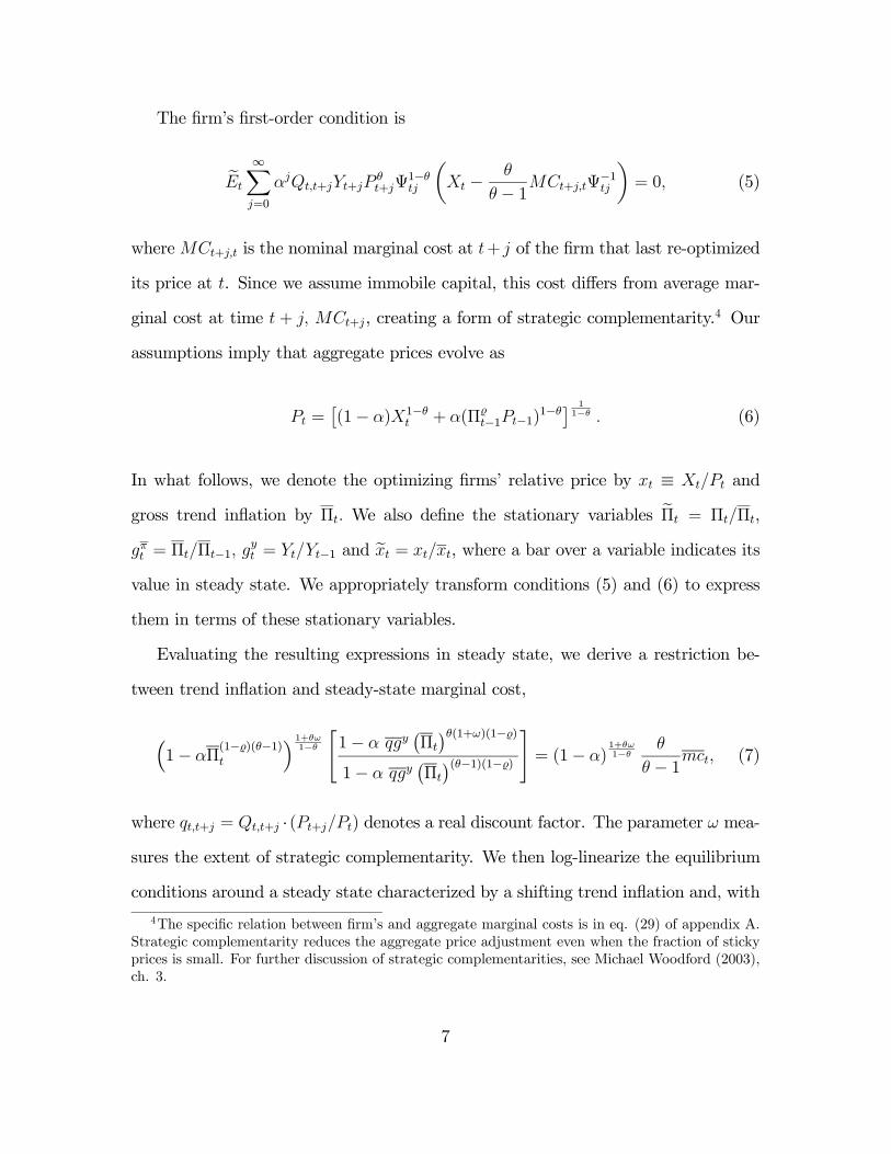
The firm’s first-order condition is

eEt

∞Xj=0

αjQt,t+jYt+jPθt+jΨ

1−θtj

µXt − θ

θ − 1MCt+j,tΨ−1tj

¶= 0, (5)

whereMCt+j,t is the nominal marginal cost at t+ j of the firm that last re-optimized

its price at t. Since we assume immobile capital, this cost differs from average mar-

ginal cost at time t + j, MCt+j, creating a form of strategic complementarity.4 Our

assumptions imply that aggregate prices evolve as

Pt =£(1− α)X1−θ

t + α(Πt−1Pt−1)1−θ¤ 11−θ . (6)

In what follows, we denote the optimizing firms’ relative price by xt ≡ Xt/Pt and

gross trend inflation by Πt. We also define the stationary variables eΠt = Πt/Πt,

gπt = Πt/Πt−1, gyt = Yt/Yt−1 and ext = xt/xt, where a bar over a variable indicates its

value in steady state. We appropriately transform conditions (5) and (6) to express

them in terms of these stationary variables.

Evaluating the resulting expressions in steady state, we derive a restriction be-

tween trend inflation and steady-state marginal cost,

³1− αΠ

(1− )(θ−1)t

´ 1+θω1−θ

"1− α qgy

¡Πt

¢θ(1+ω)(1− )

1− α qgy¡Πt

¢(θ−1)(1− )

#= (1− α)

1+θω1−θ

θ

θ − 1mct, (7)

where qt,t+j = Qt,t+j · (Pt+j/Pt) denotes a real discount factor. The parameter ω mea-

sures the extent of strategic complementarity. We then log-linearize the equilibrium

conditions around a steady state characterized by a shifting trend inflation and, with

4The specific relation between firm’s and aggregate marginal costs is in eq. (29) of appendix A.Strategic complementarity reduces the aggregate price adjustment even when the fraction of stickyprices is small. For further discussion of strategic complementarities, see Michael Woodford (2003),ch. 3.

7

usual manipulations, derive a version of the NKPC which can be written in a familiar

form as5

bπt = et ¡bπt−1 − bgπt ¢+ ζtcmct + b1t eEtbπt+1 + b2t eEt

∞Xj=2

ϕj−11t bπt+j (8)

+b3t eEt

∞Xj=0

ϕj1t

³ bQt+j,t+j+1 + bgyt+j+1´+ ut.

Hatted variables denote log-deviations of stationary variables from their steady state

values.6 An error term ut is included to account for the fact that this equation is

an approximation and to allow for other possible mis-specifications. In what follows,

we assume that ut is a white noise process. We discuss later the validity of this

assumption.

This equation differs from conventional versions of the NKPC in two respects.

First, a number of additional variables appear on the right-hand side of (8). These

include innovations to trend inflation bgπt , higher-order leads of expected inflation,and terms involving the discount factor bQt and real output growth bgyt . Excludingthese variables when estimating traditional Calvo equations would result in omitted-

variable bias on the coefficients on marginal cost and lagged inflation if the omitted

terms are correlated with those variables.

Second, the coefficients et, ζt, b1t, b2t, b3t, and ϕ1t are non-linear functions of

5A technical issue arises here, because multi-step expectations are difficult to evaluate whenparameters drift. We invoke an approximation that is standard in the macro learning literature(e.g., see George W. Evans and Seppo Honkapohja 2001): we assume that agents treat driftingparameters as if they would remain constant at the current level going forward in time. David M.Kreps (1998) refers to this assumption as an ‘anticipated-utility’ model, and he recommends it asa way to model bounded rationality. Cogley and Sargent (2006) defend it as an approximation toBayesian forecasting and decision making in high-dimensional state spaces. That approximationis very good in models which assume certainty equivalence. Our formulation implicitly assumescertainty equivalence because we log-linearize the firm’s first-order conditions.

6Specifically, bπt = ln¡Πt/Πt

¢, cmct = ln(mct/mct), bQt,t+1 = ln

¡Qt,t+1/Qt,t+1

¢, bgπt =

ln¡Πt/Πt−1

¢and bgyt = ln (gyt /gy) . In the derivation we use the fact that the discount factor between

time t and time t+ j is Qt,t+j = Πj−1k=0Qt+k,t+k+1.

8

trend inflation and the parameters of the pricing model α, , θ, and ω (their exact

expressions are given in equation (49) of appendix A). When trend inflation drifts, the

coefficients of equation (8) also drift (provided 6= 1), even if the underlying Calvoparameters are constant. In other words, although α, , θ, and ω might be invariant

to shifts in trend inflation, the NKPC parameters et, ζt, b1t, b2t, b3t, and ϕ1t are not.In particular, higher trend inflation implies a lower weight on current marginal cost

and a greater weight on expected future inflation.

The standard NKPC emerges as a special case when steady-state inflation is zero

or when there is full indexation ( = 1). In those cases, b2t = b3t = 0, while the other

coefficients collapse to those of the standard model. Another popular specification

is also nested in eq. (8). If one assumes that non-optimized prices are fully indexed

to a mixture of current trend inflation and one-period lagged inflation, the equation

collapses to a form similar to the traditional NKPC, with constant coefficients and

no extra forward-looking terms. In that case, a traditional NKPC formulation can

be obtained simply by re-defining the inflation gap as bπt = πt − πt−1 − (1− )πt.

II Econometric Approach

Our objective is to estimate the underlying parameters of the Calvo model α, ,

and θ, which govern key behavioral attributes involving the frequency of price ad-

justment, the extent of indexation to past inflation, and the elasticity of demand.

Combined with an evolving trend inflation, these parameters allow us to trace a time

path for the drifting NKPC coefficients.

Our econometric approach exploits a set of cross-equation restrictions between

the parameters of the Calvo model and those of a reduced-form vector autoregression

with drifting parameters. That the reduced-form V AR has drifting parameters follows

9

from our assumption that trend inflation drifts. In our model, the NKPC coefficients

depend on Πt. Hence, drift in trend inflation induces drift in these coefficients. It

follows that the reduced form of any structural model containing our version of the

NKPC also has time-varying parameters. Among other things, we use this V AR to

construct a measure of trend inflation and to represent agents’ subjective beliefs.7

If inflation is indeed determined in accordance with the NKPC, the V AR should

also satisfy a collection of nonlinear cross-equation restrictions. These are embedded

in two relationships derived in the previous section, one involving the cyclical com-

ponents of inflation and marginal cost (eq. 8) and the other connecting the evolution

of steady-state values (eq. 7). These relations involve non-linear combinations of the

underlying the parameters of the Calvo model (see definitions (49) in the appendix),

which we collect in a vector ψ = [α,θ, ,ω]0.

To derive the cross-equation restrictions, we consider first the case where the

V AR has constant parameters and then show its extension to the case of a V AR

with random coefficients.

Suppose the joint representation of the vector time series xt = (πt,mct, Qt, gyt )0 is

a V AR(p). Then, defining a vector zt = (xt, xt−1, ...,xt−p+1)0, we can write the law

of motion of zt in companion form as

zt= μ+Azt−1+εzt. (9)

If the NKPC model is correct, reduced-form and structural forecasts of the inflation

7The assumption that agents form expectations with a forecasting VAR is common in the learningliterature. The forecast is a ‘perceived’ law of motion (e.g. Fabio Milani 2007), and its coefficients,as ours, evolve over time. In the learning literature the time drift in the parameters is interpretedas updating of beliefs when more observations become available.

10

gap should coincide. The reduced-form conditional expectation of bπt iseE (bπt|bzt−1) = e0πAbzt−1, (10)

where ek represents a selection vector that picks up variable k in vector zt and bzt =zt−μz, where μz = (I−A)−1μ. Similarly, the conditional expectation for the inflationgap from the NKPC is

eE (bπt|bzt−1) = ee0πbzt−1 + ζe0mcAbzt−1 + b1e0πA

2bzt−1 + b2e0πϕ1(I− ϕ1A)

−1A3bzt−1+b3

¡e0Q (I− ϕ1A)

−1A+ e0y(I− ϕ1A)−1A2

¢bzt−1. (11)

After equating the two and imposing that they hold for all realizations of zt, we

obtain a vector of nonlinear cross-equation restrictions involving the parameters of

the Calvo model ψ and the VAR parameters μ and A:

e0πA = ee0πI+ ζe0mcA+ b1e0πA

2 + b2e0πϕ1(I− ϕ1A)

−1A3

+b3¡e0Q (I− ϕ1A)

−1A+ e0y(I− ϕ1A)−1A2

¢(12)

≡ g(μ,A,ψ),

or

z1(μ,A,ψ) = e0πA− g(μ,A,ψ) = 0. (13)

The parameters must also satisfy the steady state restriction (7), which we re-write

as

z2(μ,A,ψ) =³1− αΠ

(1− )(θ−1)t

´ 1+θω1−θ

"1− α qgy

¡Πt

¢θ(1+ω)(1− )

1− α qgy¡Πt

¢(θ−1)(1− )

#− (1− α)

1−θ1+θω

θ

θ − 1mct

= 0, (14)

11

where Πt andmct are the steady-state values of gross inflation and real marginal cost,

respectively, implied by the VAR. We consolidate these two moment conditions by

defining z (μ,A,ψ) = (z01 z02)0. If the model is true, there exist values of μ,A,ψ

that set z (μ,A,ψ) = 0.

With drifting parameters, we modify the previous formulas by adding time sub-

scripts to the companion form,

zt = μt +Atzt−1 + εzt, (15)

and appropriately redefining the function z as zt(μt,At,ψ) to represent the restric-

tions at a particular date. Stacking the residuals from each date into a long vector,

F(·) = [z01,z02, ...,z0T ]0 , (16)

we seek values of μt,At, and ψ for which F(·) = 0.Ideally, we would like to estimate the joint Bayesian posterior for V AR and pa-

rameters of the Calvo model, but that proved to be computationally intractable. In

Timothy Cogley and Argia M. Sbordone (2006), we outlined a Markov Chain Monte

Carlo algorithm for simulating the joint posterior of this model, but upon further

investigation we discovered that our algorithm did not converge. We tried to repair

this defect but were unable to resolve the problem.8 Since we are unable to simulate

8The convergence problem most likely follows from the existence of multiple solutions to (13) and(14). Roughly speaking, the algorithm fails to converge because it keeps switching across solutions,staying in the neighborhood of one for a long time, then switching to another. One branch —described in our earlier paper — makes economic sense, but the others do not. We experimentedwith a number of devices for eliminating the ill-behaved branches but failed to find one that made thealgorithm converge. Among other things, we considered a particle filter, following Jesus Fernandez-Villaverde and Juan Rubio-Ramirez (2007), but we decided against it because it is not promisingfor our model. The regularity conditions underlying the particle filter presume a unique solution toequations corresponding to (13) and (14) (assumption 2 of Fernandez-Villaverde and Rubio-Ramirez,2007). In addition, our model is more complex than theirs in one key dimension. For computational

12

the posterior, we resort to a shortcut.

Following Sbordone (2002, 2006), we adopt a two-step estimation procedure. First,

we fit to the data an unrestricted reduced-form V AR. Then, conditional on those

estimates, we search for values of the parameters ψ that make z (ψ) close to zero,

where ‘close’ is defined in terms of an unweighted sum-of-squares

bψ = argminz³bμt, At,ψ´0z³bμt, At,ψ

´. (17)

Estimation of the first-stage V AR follows Cogley and Sargent (2005a) and delivers

a sample from the Bayesian posterior for μ,A. The second stage defines an implicit

function that maps the V AR parameters into best-fitting values for the parameters of

the Calvo model. We view this as a change of variables ψ = h(μ,A) which transforms

the posterior sample for the V AR parameters into a sample for the parameters of the

pricing model. Thus, for each draw in the posterior for μ,A, we find the best-fitting

value for ψ by solving (17). In this way, we induce a distribution for ψ from the

distribution for μ,A.

This procedure does not deliver a Bayesian posterior for ψ, but it is logically

coherent. Our inferences about ψ are suboptimal because they do not follow from

Bayes’ theorem. Essentially, we are using the likelihood function for an unrestricted

VAR to learn about parameters of a restricted VAR. We would prefer to simulate

the posterior for the restricted VAR, but since we cannot, we adopt this two-step

estimator as a second-best approach.

Nevertheless, we conjecture that the Bayesian posterior for μ,A,ψ would not

differ greatly from the estimates reported below. This is based on the fact that the

unrestricted VAR comes close to satisfying the cross-equation restrictions (evidence

reasons, they permit only one parameter to drift, while in our model the entire V AR parametervector is free to drift.

13

on this is reported below). That being the case, we suspect that the likelihoods

for the restricted and unrestricted models are not terribly different. To verify this

conjecture, we would have to simulate the posterior for the restricted VAR, which, as

said, we are currently unable to do. We leave this for future research.

III The First-Stage VAR

When trend inflation is non-zero, inflation depends not only on the evolution of

marginal costs but also on expectations of output growth and the discount rate. We

therefore estimate a vector autoregression for inflation, log marginal cost, output

growth, and a nominal discount factor. We allow for changes in the law of motion of

these variables by estimating aVAR with drifting parameters and stochastic volatility.

In this section, we describe the data, how the VAR is specified, and how the model

is estimated.

A The Data

Inflation is measured from the implicit GDP deflator, recorded in NIPA table 1.3.4.

Output growth is calculated using chain-weighted real GDP, expressed in 2000$, and

seasonally adjusted at an annual rate. This series is recorded in NIPA table 1.3.6.

The nominal discount factor is constructed by expressing the federal funds rate on

a discount basis. Federal funds data are monthly averages of daily figures and were

converted to quarterly values by point-sampling the middle month of each quarter.

Marginal cost is approximated by unit labor cost. This is correct under the

hypothesis of Cobb-Douglas technology: in this case the marginal product of labor is

proportional to the average product, and real marginal cost (mct) is proportional to

14

unit labor cost,

mct = wtHt/(1− δ)PtYt = (1− δ)−1ulct, (18)

where (1− δ) is the output elasticity to hours of work in the production function.

Because we exploit a restriction on trend marginal cost mct (eq. (14)), we need a

measure of unit labor costs in natural units rather than as index number. To construct

such a measure, we compute an index of total compensation in the non-farm business

sector from BLS indices of nominal compensation and total hours of work, then

translate the result into dollars.9 A (log) measure of real unit labor cost ulc is then

obtained by subtracting (log of) nominal GDP from (log of) labor compensation.

The new measure of ulc correlates almost perfectly with the BLS index number for

unit labor cost in the non-farm business sector, another measure commonly used in

the literature (e.g., see Sbordone 2002, 2006). Finally, to transform the real unit

labor cost (or labor share) into real marginal cost, we subtract the log exponent on

labor, (1− δ) , which we calibrate at 0.7.

The sample covers the period 1954.Q1 to 2003.Q4. Data from 1954.Q1-1959.Q4

are used to initialize the prior, and the model is estimated using data from 1960.Q1

through 2003.Q4.

B The VAR Specification

The reduced-form specification follows Cogley and Sargent (2005a). We write the

V AR as

xt = X0tϑt + εxt, (19)

9Because we lack the right data for the non-farm business sector, we perform the translationusing data for private sector labor compensation, which we obtained from table B28 of the EconomicReport of the President (2004). From that table, we calculated total labor compensation in dollarsfor 2002; the number for that year comes to $4978.61 billion. The BLS compensation index is thenrescaled so that the new compensation series has that value in 2002.

15

where xt is a N × 1 vector of endogenous variables (N = 4 in our case), X0t =

IN ⊗£1 x0t−l

¤, where x0t−l represents lagged values of xt and ϑt denotes a vector

of time-varying conditional mean parameters. In the companion-form notation used

above, the matrix At refers to the autoregressive parameters in ϑt, and the vector μt

includes the intercepts.

As in Cogley and Sargent, ϑt is assumed to evolve as a driftless random walk

subject to reflecting barriers. Apart from the reflecting barrier, ϑt evolves as

ϑt = ϑt−1 + vt. (20)

The innovation vt is normally distributed, with mean 0 and variance Ω. Denoting by

ϑT the history of V AR parameters from date 1 to T , ϑT = [ϑ01, ...,ϑ0T ]0, the driftless

random walk component is represented by a joint prior

f¡ϑT ,Ω

¢= f

¡ϑT |Ω¢ f (Ω) = f (Ω)

T−1Ys=0

f (ϑs+1|ϑs,Ω) . (21)

Associated with this is a marginal prior f(Ω) that makes Ω an inverse-Wishart vari-

ate.

The reflecting barrier is encoded in an indicator function, I(ϑT ) =QT

s=1 I(ϑs).

The function I(ϑs) takes a value of 0 when the roots of the associated V AR polyno-

mial are inside the unit circle, and it is equal to 1 otherwise. This restriction truncates

and renormalizes the random walk prior, p(ϑT ,Ω)∝ I(ϑT )f(ϑT ,Ω). This represents

a stability condition for the V AR, which rules out explosive representations for the

variables in question.10

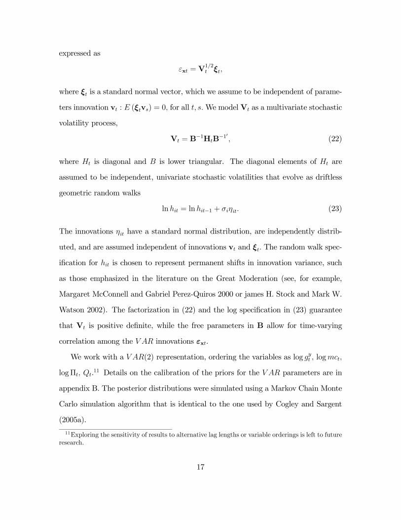
To allow for stochastic volatility, we assume that the V AR innovations εxt can be

10Explosive representations might be useful for modeling hyperinflationary economies, but weregard them as implausible for the post World War II U.S.

16

expressed as

εxt = V1/2t ξt,

where ξt is a standard normal vector, which we assume to be independent of parame-

ters innovation vt : E (ξtvs) = 0, for all t, s.We modelVt as a multivariate stochastic

volatility process,

Vt = B−1HtB

−10 , (22)

where Ht is diagonal and B is lower triangular. The diagonal elements of Ht are

assumed to be independent, univariate stochastic volatilities that evolve as driftless

geometric random walks

lnhit = lnhit−1 + σiηit. (23)

The innovations ηit have a standard normal distribution, are independently distrib-

uted, and are assumed independent of innovations vt and ξt. The random walk spec-

ification for hit is chosen to represent permanent shifts in innovation variance, such

as those emphasized in the literature on the Great Moderation (see, for example,

Margaret McConnell and Gabriel Perez-Quiros 2000 or james H. Stock and Mark W.

Watson 2002). The factorization in (22) and the log specification in (23) guarantee

that Vt is positive definite, while the free parameters in B allow for time-varying

correlation among the V AR innovations εxt.

We work with a V AR(2) representation, ordering the variables as log gyt , logmct,

logΠt, Qt.11 Details on the calibration of the priors for the V AR parameters are in

appendix B. The posterior distributions were simulated using a Markov Chain Monte

Carlo simulation algorithm that is identical to the one used by Cogley and Sargent

(2005a).

11Exploring the sensitivity of results to alternative lag lengths or variable orderings is left to futureresearch.

17

C Trend Inflation and Persistence of the Inflation Gap

Two features of the VAR are relevant for the NKPC, namely, how trend inflation

varies and how that variation alters inflation-gap persistence. Following S. Beveridge

and C. R. Nelson (1981), we define trend inflation as the level to which inflation

is expected to settle after short-run fluctuations die out, πt = limj→∞Etπt+j. We

approximate this by calculating a local-to-date t estimate of mean inflation from the

V AR,

πt = e0π(I−At)−1μt. (24)

In general equilibrium, mean inflation is usually pinned down by the target in the

central bank’s policy rule. Accordingly, we interpret movements in πt as reflecting

changes in this aspect of monetary policy.12

Figure 1 portrays the median estimate of trend inflation at each date, shown as a

dotted line, and compares it with actual and mean inflation. The latter are recorded

as solid and dashed lines, respectively, and all are expressed at annual rates. The

estimates are conditioned on data through the end of the sample, so we denote them

πt|T .

Two features of the graph are relevant for what comes later. The first, of course,

is that trend inflation varies. We estimate that it rose from 2.3 percent in the early

1960s to roughly 4.75 percent in the 1970s, then fell to around 1.65 percent at the end

of the sample. A time-varying inflation trend makes our inflation gap quite different

from those in conventional Calvo models. We measure the inflation gap as deviation of

inflation from the time-varying trend, πt− πt|T . By contrast, in conventional versions12Notice that πt is a driftless random walk to a first-order approximation: this follows from the fact

that a first-order Taylor expansion makes πt linear in the VAR parameter vector ϑt, which evolvesas driftless random walk when away from the reflecting barrier. In this respect, our specificationagrees with that of the inflation target in Ireland (2007).

18

1960 1965 1970 1975 1980 1985 1990 1995 2000 2005

0

0.02

0.04

0.06

0.08

0.1

0.12

0.14

InflationMean Inflation,Trend Inflation

Figure 1: Inflation, Mean Inflation, and Trend Inflation

of the Calvo model, the inflation gap is measured as the deviation from a constant

mean, reflecting the assumption of a constant steady-state rate of inflation. The

measurement of the inflation gap matters a great deal because it affects the degree

of persistence. As the figure illustrates, the mean-based gap is more persistent than

trend-based measures. Notice, for example, the long runs at the beginning, middle,

and end of the sample when inflation does not cross the mean. In contrast, inflation

crosses the trend line more often, especially after the Volcker disinflation.

Table 1 summarizes the autocorrelation of the inflation gap. The first row refers to

actual inflation. For this measure, trend inflation is just the sample average, and the

inflation gap is the deviation from the mean. The autocorrelation hovers around 0.8

both for the whole sample and for the two subsamples. In the second row, the inflation

gap is measured by subtracting the median estimate of trend inflation from actual

inflation. This matters only slightly for the period before the Volcker disinflation, but

afterwards the autocorrelation of the inflation gap is reduced substantially, to around

0.3.13

13Cogley, Primiceri, and Sargent (2007) investigate this issue more rigorously and conclude thatinflation-gap persistence was significantly lower after the Volcker disinflation.

19

Table 1: Autocorrelation of the Inflation Gap

1960-2003 1960-1983 1984-2003

Inflation 0.834 0.843 0.784

Trend-Based Gap 0.769 0.801 0.305

Purely forward-looking versions of the Calvo model are often criticized for gener-

ating too little persistence and, accordingly, the model is modified by introducing a

backward-looking element. The table and figure make us wonder whether this ‘excess

persistence’ reflects an exaggeration of the persistence in mean-based measures of the

gap rather than a deficiency of persistence in forward-looking models. In particular,

if the trend-based measure is right, for the period after 1984 the NKPC needs to

explain only a modest degree of persistence. A purely forward-looking version may

be adequate after all.

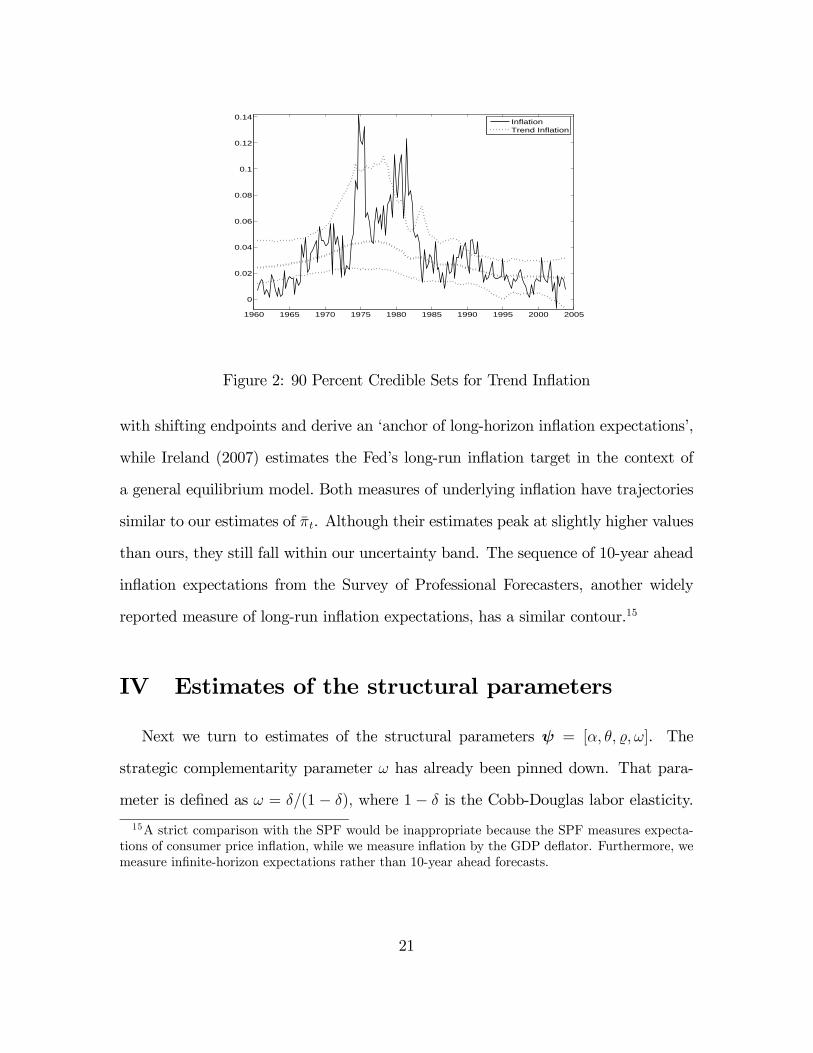
While figure 1 is suggestive, one should not attach too much significance to the

particular path for πt|T shown there. On the contrary, there is a lot of uncertainty

about the level of trend inflation at any given date. Figure 2 conveys a sense of

this uncertainty by displaying marginal 90 percent credible sets at each date.14 The

credible sets are widest during the Great Inflation and are narrower when trend

inflation is low. Our estimates of the structural parameters take this uncertainty into

account because they are based on the entire posterior sample for trend inflation,

not just on the mean or median path.Nevertheless, it is worth pointing out that

other measures proposed in the literature are roughly in line with our estimates. For

instance, Sharon Kozicki and Peter A. Tinsley (2002) estimate a multivariate V AR

14A credible set is a Bayesian analog to a confidence interval. The marginal credible sets portrayuncertainty about the location of πt at a given date. However, the figure does not address whetherchanges in πt across time are statistically significant. Cogley, Primiceri, and Sargent (2007) elaborateon this point.

20

1960 1965 1970 1975 1980 1985 1990 1995 2000 2005

0

0.02

0.04

0.06

0.08

0.1

0.12

0.14

InflationTrend Inflation

Figure 2: 90 Percent Credible Sets for Trend Inflation

with shifting endpoints and derive an ‘anchor of long-horizon inflation expectations’,

while Ireland (2007) estimates the Fed’s long-run inflation target in the context of

a general equilibrium model. Both measures of underlying inflation have trajectories

similar to our estimates of πt. Although their estimates peak at slightly higher values

than ours, they still fall within our uncertainty band. The sequence of 10-year ahead

inflation expectations from the Survey of Professional Forecasters, another widely

reported measure of long-run inflation expectations, has a similar contour.15

IV Estimates of the structural parameters

Next we turn to estimates of the structural parameters ψ = [α, θ, , ω]. The

strategic complementarity parameter ω has already been pinned down. That para-

meter is defined as ω = δ/(1− δ), where 1− δ is the Cobb-Douglas labor elasticity.

15A strict comparison with the SPF would be inappropriate because the SPF measures expecta-tions of consumer price inflation, while we measure inflation by the GDP deflator. Furthermore, wemeasure infinite-horizon expectations rather than 10-year ahead forecasts.

21

We calibrated δ = 0.3 when constructing data on real marginal cost,16 and that fixes

ω = 0.429. That leaves three free parameters — α, θ, and — to estimate.

When solving the minimum-distance problem (17), we constrain α, , and θ to lie

in the economically meaningful ranges listed in table 2. We also check whether the

estimates satisfy the conditions for existence of a steady state (the inequalities (39)

and (40) in appendix A). Those conditions are satisfied for roughly 99 percent of the

draws in the Monte Carlo sample.

Table 2: Admissible Range for Estimates

α θ

(0, 1) [0, 1] (1,∞)

Table 3 summarizes the second-stage estimates. Because the distributions are

non-normal, the table records the median and 90 percent confidence intervals. The

estimates are economically sensible, they accord well with microeconomic evidence,

and they are reasonably precise.

Table 3: Estimates of the Structural Parameters

α θ

Median

90 percent Confidence Interval

0.588

(0.44,0.70)

0

(0,0.15)

9.8

(7.4,12.1)

Since our main interest is to assess the importance of a backward-looking com-

ponent, an especially interesting outcome concerns the indexation parameter, whose

16See section 4.1. The results we report below about are robust to other plausible values of δ,and the estimates of α and θ are only marginally affected (an increase in δ tends to lower α andraise θ).

22

median estimate is 0. Approximately 78 percent of the estimates lie exactly on the

lower bound of 0, and 90 percent are less than 0.15. This contrasts with much of

the empirical literature based on time-invariant models in which the indexation pa-

rameter is estimated as low as 0.2 and as high as 1, and is statistically significant.

For instance, when estimating a wage-price system, Sbordone (2006) estimates values

for ranging from 0.15 to 0.22, depending on the VAR specification. In a general

equilibrium model, Frank Smets and Rafael Wouters (2007) estimate a value of ap-

proximately 0.25. Marc Giannoni and Michael Woodford (2003) estimate a value

close to 1, and Christiano, Eichenbaum, and Evans (2005) set exactly equal to 1.

Marco Del Negro and Frank Schorfheide (2006) also find the parameter concen-

trating near zero, but they need highly autocorrelated mark-up shocks to obtain this

result. In contrast, we reconcile = 0 with a white noise mark-up shock. Other au-

thors, following Gali and Gertler (1999), introduce a role for past inflation assuming

the presence of rule-of-thumb firms, instead of assuming indexation, and similarly

estimate significant coefficients on lagged inflation. In those models, an important

backward-looking component is needed to fit inflation persistence, but that is not the

case here.

In our model the persistence of trend inflation explains most of the persistence in

inflation, which makes it easier to fit data on the inflation gap πt − πt with a purely

forward-looking model. Secondly, there is no need for a backward-looking term be-

cause we appropriately account for time-variation in πt. Our approximation implies

that the NKPC includes additional leads of inflation, rather than lags, and these

have more weight the higher is trend inflation. Since these forward-looking terms

are positively correlated with past inflation (as must be true when inflation predicts

future inflation more than one quarter ahead and Granger-causes output growth and

the nominal interest rate), their omission could spuriously generate a positive coeffi-

23

cient on lagged inflation in estimates of the hybrid NKPC. This artificial inflation

persistence creates a ‘persistence puzzle’ for forward-looking models of inflation gaps

relative to a constant long-run average inflation rate.17

At this point, we must temper our conclusion about by acknowledging an iden-

tification problem. Andreas Beyer and Roger E.A. Farmer (2007) demonstrate that

identification of forward and backward-looking terms in the NKPC depends on as-

sumptions about other structural equations in a general equilibrium model. When

those equations are unspecified — as they are here — identification hinges on auxiliary

assumptions about features such as V AR lag length and/or the autocorrelation prop-

erties of the cost-push shock. Thus, in a fundamental sense, whether our estimates

are supported by convincing economic restrictions is not clear.

This issue is difficult to resolve using macro data alone, but micro data provide

some help. Bils and Klenow (2004) report a median duration of prices of 4.4 months

for a sample period covering 1995-97, and Nakamura and Steinsson (2007) obtain

similar results for two longer samples, covering 1988-97 and 1998-05, respectively.

Specifications of the Calvo model involving an indexation component are hard to

reconcile with their evidence. When > 0, every firm changes price every quarter,

some optimally rebalancing marginal benefit and marginal cost, others mechanically

marking up prices in accordance with the indexation rule. Unless the optimal re-

balancing happened to result in a zero price change or lagged inflation were exactly

zero, conditions that are very unlikely, no firm would fail to adjust its nominal price.

In a world such as that, Bils-Klenow and Nakamura-Steinsson would not have found

that a large fraction of prices remain unchanged each month. We interpret this as

17Ireland (2007) also finds no role for indexation to past inflation when trend inflation is allowedto drift. His hypothesis for why trend inflation alters the NKPC, however, is different from ours,since it is due to indexation of non-optimally reset prices to trend inflation.

24

additional evidence in support of a purely forward-looking model.18

Turning to the degree of nominal rigidity, our median estimate for the fraction of

sticky-price firms is α = 0.588 per quarter, with a 90 percent confidence interval of

(0.44, 0.70). In conjunction with the estimate of = 0, our point estimate implies

a median duration19 of prices of 1.31 quarters, or 3.9 months, with a 90 percent

confidence interval ranging from 2.5 to 5.8 months. Thus, our estimates are not far

from the unadjusted estimates of Bils and Klenow (2004) and Nakamura and Steinsson

(2007). Results from micro studies are sensitive, however, to the treatment of sales

and product substitution. For instance, Bils and Klenow report that the median

duration increases to 5.5 months after removing sales price changes. In contrast,

Nakamura and Steinsson (2007) find a longer median duration of about 8 months

after excluding sales and product substitutions. Bils and Klenow’s adjusted estimate

is close to the upper end of our confidence interval, but the Nakamura-Steinsson

number lies outside.

Finally, the median estimate of θ implies a steady-state markup of about 11 per-

cent, which is in line with other estimates in the literature. For example, this is

the same order of magnitude as markups estimated by Susanto Basu (1996) and Su-

santo Basu and Miles Kimball (1997) using sectoral data. With economy-wide data,

in the context of general equilibrium models, estimates range from around 6 to 23

percent, depending on the type of frictions in the model. Julio J. Rotemberg and

Michael Woodford (1997) estimate a steady state markup of 15 percent (θ ≈ 7.8).Jeffrey D. Amato and Thomas Laubach (2003), in an extended model which include

18It should be noted, however, that the introduction of a backward-looking component throughrule-of-thumb behavior, as in Gali and Gertler (1999), does not suffer from this problem. In thosemodels, a fraction α of firms does maintain prices unchanged in each quarter.19For a purely forward-looking Calvo model, the waiting time to the next price change can be

approximated as αt, and from that one can calculate that the median waiting time is -ln(2)/ln(α).The median waiting time is less than the mean because the distribution of waiting times has a longupper tail.

25

also wage rigidity, estimate a steady-state markup of 19 percent. Rochelle M. Edge,

Thomas Laubach and John C. Williams (2003) find a slightly higher value, 22.7 per-

cent (θ = 5.41). The estimates in Christiano, Eichenbaum and Evans (2005) span

a larger range, varying from around 6.35 to 20 percent, depending on details of the

model specification. We conclude that, although obtained through a different esti-

mation strategy, our markup estimate falls within the range found by others.

We should at this point comment on another identification issue. As pointed

out earlier in the literature and recently emphasized by Martin Eichenbaum and

Jonas Fisher (2007), in standard Calvo models the contributions of real and nominal

rigidities to the coefficient on marginal cost may not be separately identified. But in

our generalized Calvo model we are indeed able to identify all three parameters of

interest: , α, and θ.20 The question is then which features of this model allow the

identification.

In order to explore this issue, we estimated nested versions of the model, pro-

gressively turning off various of its features one at the time. First, we estimated the

model omitting terms involving the discount factor and output growth. As expected,

these terms do not matter, and the estimates are unaffected (see table C.1 in the

appendix). Next, we also omitted terms involving higher-order leads of inflation.

Again, the estimates are unaffected (see table C.2). We then deactivated also the

dependence of the NKPC coefficients upon trend inflation, obtaining a representa-

tion resembling a model involving a mixed form of indexation, as discussed earlier.

In this case, the estimates of α and θ are marginally affected, but remains concen-

trated on zero (see table C.3). All these estimates were obtained using both sets of

cross-equation restrictions, i.e. those linking the steady-state values of inflation and

marginal cost (eq. (14)), as well as those involving deviations from the steady state

20As we pointed out before, these estimates are conditional on the calibrated value of ω.

26

(eq. (12)). If, in addition, we deactivate either set of restrictions, the model seems to

be under-identified, and the numerical optimizer frequently fails to find a minimum.

We conclude that two features matter for identification, viz. time variation in πt and

At and the use of additional cross-equation restrictions coming from the steady-state

relationship.

The model is overidentified, with 3 free parameters to fit 9·T elements in F (·) .However, in this environment we cannot justify the conventional J-test for overidenti-

fying restrictions. To provide an overall measure of fit, we follow Campbell and Shiller

(1987) by informally comparing the expected inflation gap implied by the NKPC and

the unconstrained V AR. The VAR inflation forecast is given by equation (10), while

the NKPC forecast is implicitly defined by the right-hand-side of equation (11). The

distance between the two measures the extent to which the cross-equation restrictions

are violated.

The top panel of figure 3 plots the two series, showing VAR and NKPC forecasts

as solid and dotted lines, respectively. To calculate the two forecasts, we condition

on median estimates of the VAR and Calvo parameters. As the figure shows, NKPC

forecasts closely track those of the unrestrictedVAR. The two series have a correlation

of 0.978, and the deviations between them are small in magnitude and represent high-

frequency twists and turns.

The bottom panel looks more closely at the distance between (10) and (11). For

that panel, we calculate cross-equation errors for every draw in the Monte Carlo

sample and then plot a 90 percent marginal confidence interval for each date. Except

for a handful of dates, those confidence intervals include zero. Hence, there is little

evidence against the model’s cross-equation restrictions.

Finally, we revisit the assumption that the cost-push shock ut is unforecastable.

Remember that we assumed that E (ut|bzt−1) = 0. If we measure ut as the residual

27

1960 1970 1980 1990 2000 2010−0.05

0

0.05

0.1

0.15A Campbell−Shiller Graph

VAR Expected InflationNKPC Expected Inflation

1960 1970 1980 1990 2000 2010−0.04

−0.02

0

0.02

0.04Date−by−Date Confidence Intervals for Cross−Equation Errors

Correlation = 0.978

Figure 3: Assessing the Cross-Equation Restrictions

in (8) and take its expectation with respect to the right-hand side variables in the

VAR, bzt−1, we obtain equation (11).21 Therefore, the question of predictability in

ut is closely connected to the validity of the cross-equation restrictions. Intuitively,

predictable movements in ut would drive a wedge between the left- and right-hand

sides of (12), so if ut were forecastable, the VAR would not satisfy the NKPC cross-

equation restrictions. The deviations shown in figure 3 can indeed be interpreted

as a measure of this wedge. Because those discrepancies are small, it follows that

predictable movements in ut must also be small. Hence, there is little evidence against

the assumption that ut is white noise.

21As before, that expectation is taken with respect to the time-varying law of motion (μt,At),and we use the ‘anticipated-utility’ approximation for nonlinear terms.

28

1960 1970 1980 1990 20000

0.02

0.04

0.06

ζt

1960 1970 1980 1990 20000.95

1

1.05

1.1

b1t

1960 1970 1980 1990 2000

0

0.02

0.04

b2t

1960 1970 1980 1990 2000

0

5

10x 10

−3 b3t

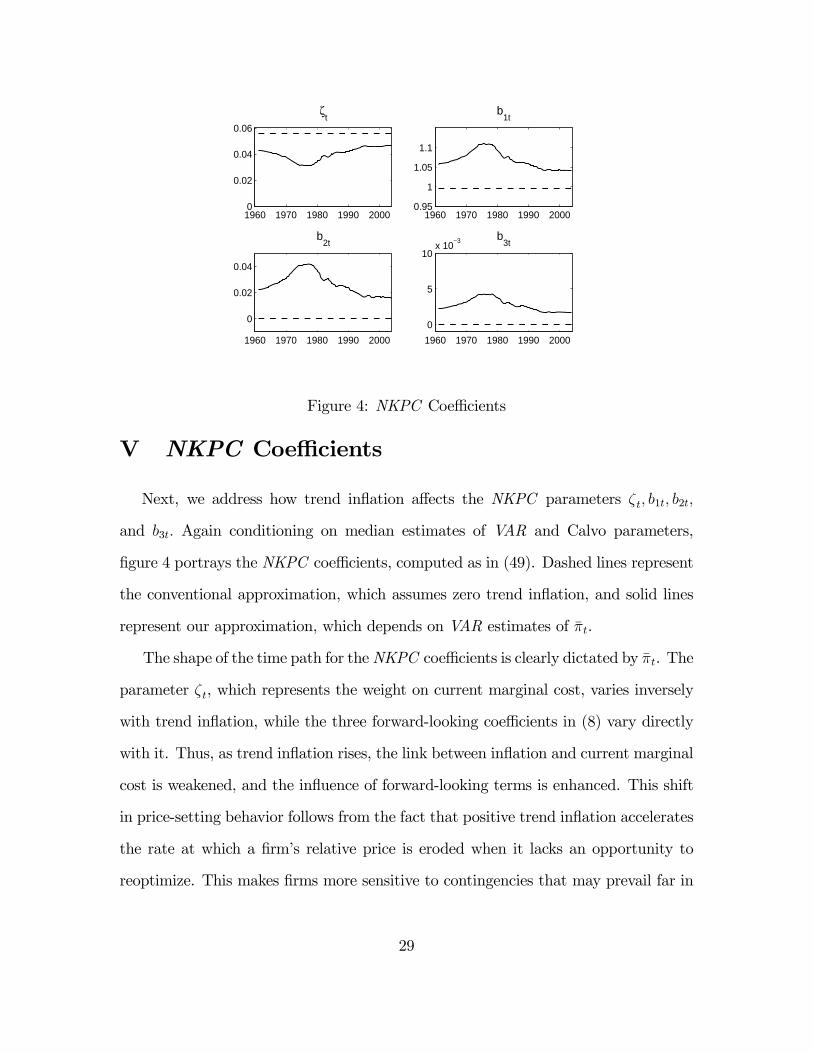
Figure 4: NKPC Coefficients

V NKPC Coefficients

Next, we address how trend inflation affects the NKPC parameters ζt, b1t, b2t,

and b3t. Again conditioning on median estimates of VAR and Calvo parameters,

figure 4 portrays the NKPC coefficients, computed as in (49). Dashed lines represent

the conventional approximation, which assumes zero trend inflation, and solid lines

represent our approximation, which depends on VAR estimates of πt.

The shape of the time path for theNKPC coefficients is clearly dictated by πt. The

parameter ζt, which represents the weight on current marginal cost, varies inversely

with trend inflation, while the three forward-looking coefficients in (8) vary directly

with it. Thus, as trend inflation rises, the link between inflation and current marginal

cost is weakened, and the influence of forward-looking terms is enhanced. This shift

in price-setting behavior follows from the fact that positive trend inflation accelerates

the rate at which a firm’s relative price is eroded when it lacks an opportunity to

reoptimize. This makes firms more sensitive to contingencies that may prevail far in

29

the future if their price remains stuck for some time. Thus, relative to the conventional

approximation, current costs matter less and anticipations matter more.

The path for ζt echoes a point emphasized by Cogley and Sargent (2005b) and

Giorgio Primiceri (2006). They argue that the Fed’s reluctance to disinflate during

the Great Inflation was due in part to beliefs that the sacrifice ratio had increased. In

traditional Keynesian models, the sacrifice ratio depends inversely on the coefficient

on real activity. The less sensitive inflation is to current unemployment or the output

gap, the more slack will be needed to disinflate. Cogley, Sargent, and Primiceri

recursively estimate backward-looking Phillips curves and find that inflation indeed

became less sensitive to real activity during the Great Inflation. It is interesting that

estimates of our forward-looking model also point towards a decline in the coefficient

on real activity (i.e., real marginal cost) during the 1970s. In that respect, our

estimates are consistent with theirs, while providing a structural interpretation for

the declining coefficient.

Our model suggests that concerns about the slope of the short-run Phillips curve

might have been exaggerated because parameters like ζt are not structural. In our

model, a credible policy reform that reduced πt would increase ζt, thus making in-

flation more sensitive to current marginal cost. By assuming that parameters like

ζt were invariant to shifts in trend inflation, policy analysts in the 1970s probably

overstated the cost of a disinflationary policy.

Focusing on the forward-looking coefficients, notice that the coefficient b3t on the

terms in (8), which involve forecasts of output growth and the discount factor is

always close to zero. Hence the terms involving expectations of output growth and

the discount factor make a negligible contribution to inflation. What matters more

is how trend inflation alters the coefficients on expected inflation, b1 and b2. Figure

5 shows that b1 flips from slightly below 1 when trend inflation is zero to between

30

1.05 and 1.1 for our estimates of πt. Similarly, when trend inflation is zero, b2 is also

zero, and multi-step expectations of inflation drop out of equation (8). When trend

inflation is positive instead, those higher-order expectations enter the equation with

coefficients of 0.02-0.04.

VI Conclusion

Inflation is highly persistent, but much of that persistence is due to shifts in trend

inflation. The inflation gap — i.e., actual minus trend inflation — is less persistent

than inflation itself. Many previous papers on the NKPC neglect variation in trend

inflation and attribute all the persistence of inflation to the inflation gap. Matching

that exaggerated degree of persistence requires a backward-looking component which

is typically motivated either as reflecting indexation or rule-of-thumb behavior. Many

NewKeynesian economists are uncomfortable about the backward-looking component

because its microfoundations are less well developed than those of the forward-looking

element.

In this paper, we address whether a more exact version of the Calvo model can ex-

plain inflation dynamics without the introduction of ad hoc backward-looking terms.

We derive a version of the NKPC as an approximate equilibrium condition around

a time-varying inflation trend with coefficients that are nonlinear combinations of

the parameters describing market structure, the pricing mechanism, and trend in-

flation. We estimate the model in two steps, first estimating an unrestricted VAR

and then estimating the parameters of the pricing model by exploiting cross-equation

restrictions on the VAR parameters.

We find that no indexation or backward-looking component is needed to model

inflation dynamics once shifts in trend inflation are taken into account. The absence

31

of indexation is consistent with microeconomic evidence that some nominal prices

remain fixed for months at a time. Our estimate of the frequency of price adjustment

is also in line with estimates from micro data.

Nevertheless, our analysis could be improved in a number of ways. In particular,

we assume that the Calvo pricing parameters are invariant to shifts in trend inflation,

which cannot literally be true. In a companion paper (Cogley and Sbordone, 2005)

we explore whether that assumption is a reasonable approximation for the kind of

variation in πt seen in postwar U.S. data.

Another important extension concerns the origins of shifts in the Fed’s long-run

inflation target. Following much of the rest of the literature, we treat πt as an exoge-

nous random process.22 Since this accounts for most of the persistence in inflation,

explaining why it drifts is important. One plausible story is that the Fed updates its

policy rule as it learns about the structure of the economy and that shifts in πt are an

outcome of this process (Cogley and Sargent 2005b, Primiceri 2006, Thomas Sargent,

Noah Williams and Tao Zha 2006, and Giacomo Carboni and Martin Ellison 2007).

More work is needed to understand how this occurs.

Finally, because of computational limitations, we were forced to take econometric

shortcuts. In future research, we hope to devise efficient algorithms for simulating

the Bayesian posterior for models like this.

22Ireland (2007) explores a model where target inflation responds to exogenous supply shocks, butfinds such a model statistically indistinguishable from one with an exogenous target.

32

Appendix A: NKPC with non stationary trend in-

flation

In this appendix, we derive a log-linear approximation of the evolution of aggregate

prices and the firms’ first order conditions and explain how to combine them to obtain

the NKPC in the text.

A Log-linear approximation of the evolution of aggregate

prices

We first divide (6) by Pt to have

1 = (1− α)x1−θt + α(Πt−1Π−1t )

1−θ (25)

Then we transform (25) to express it in terms of the stationary variables defined in

the text:

1 = (1− α)x1−θt ex1−θt + αhΠ(1− )(θ−1)t

i ¡gπt¢− (1−θ) eΠ (1−θ)

t−1 eΠ−(1−θ)t . (26)

In steady state eΠt = 1 and ext = 1, and (26) defines a function xt = x¡Πt

¢

xt =

"1− αΠ

(1− )(θ−1)t

1− α

# 11−θ

. (27)

Defining hat variables bxt ≡ ln ext and bπt ≡ ln eΠt ≡ ln¡Πt/Πt

¢ ≡ πt−πt, the log-linearapproximation of (26) around its steady state is:

0 ' (1− α)x1−θt bxt − αhΠ(1− )(θ−1)t

i ¡bπt − ¡bπt−1 − bgπt ¢¢33

which, substituting (1− α)x1−θt from (27), becomes

0 'h1− αΠ

(1− )(θ−1)t

i bxt − αhΠ(1− )(θ−1)t

i ¡bπt − ¡bπt−1 − bgπt ¢¢ .This expression gives a solution for bxt as a function of bπt, bπt−1 and bgπt :

bxt = αΠ(1− )(θ−1)t

1− αΠ(1− )(θ−1)t

£bπt − ¡bπt−1 − bgπt ¢¤ = 1

ϕ0t

£bπt − ¡bπt−1 − bgπt ¢¤ , (28)

where I set ϕ0t =1−αΠ(1− )(θ−1)

t

αΠ(1− )(θ−1)t

.

B Log-linear approximation of firm’s FOC

Marginal cost at t + j of the firm that changed price at t relates to the average

marginal cost at t+ j as

MCt+j,t =MCt+j

µXΨtj

Pt+j

¶−θω=MCt+jX

−θωt Ψ−θωtj P θω

t+j (29)

where ω is the elasticity of firm’s marginal cost to its own output. Substituting this

expression in eq. (5), we have

eEt

∞Xj=0

αjQt,t+jYt+jPθt+jΨ

1−θtj

µX(1+ωθ)t − θ

θ − 1MCt+jΨ−(1+θω)tj P θω

t+j

¶= 0

which implies that

X1+ωθt =

θθ−1

eEt

∞Pj=0

αjqt,t+jYt+jPθ(1+ω)−1t+j Ψ

−θ(1+ω)tj MCt+j

eEt

∞Pj=0

αjqt,t+jYt+jPθ−1t+j Ψ

1−θtj

≡ Ct

Dt(30)

34

where we have expressed the discount factor in real terms (qt,t+j = Qt,t+jPt+jPt) and

qt,t+j =Yj−1

k=0qt+k,t+k+1. Using the definition ofΨtj in (3) we can express the functions

C and D in recursive form, respectively

Ct =θ

θ − 1YtPθ(1+ω)−1t MCt + eEt

hα qt,t+1Π

− θ(1+ω)t Ct+1

i(31)

and

Dt = YtPθ−1t + eEt

hα qt,t+1Π

(1−θ)t Dt+1

i. (32)

Deflating appropriately (31) and (32) we obtain

eCt ≡ Ct

YtPθ(1+ω)t

=θ

θ − 1mct + eEt

hα qt,t+1g

yt+1 (Πt+1)

θ(1+ω)Π− θ(1+ω)t

eCt+1

i(33)

eDt ≡ Dt

YtPθ−1t

= 1 + eEt

hα qt,t+1g

yt+1 (Πt+1)

θ−1Π (1−θ)t

eDt+1

i(34)

where mct ≡MCt/Pt and gyt+1 = Yt+1/Yt. Note that

eCteDt

=

Ct

YtPθ(1+ω)t

Dt

YtPθ−1t

=Ct

Dt

YtPθ−1t

YtPθ(1+ω)t

=Ct

Dt

1

P(1+θω)t

=

µXt

Pt

¶1+θω≡ x1+θωt . (35)

From (33) and (34) evaluated at steady state we can solve for

Ct =θ

θ−1mct

1− αqgy¡Πt

¢θ(1+ω)(1− )(36)

Dt =1

1− αqgy¡Πt

¢(θ−1)(1− )(37)

and

x1+θωt =Ct

Dt

=

"1− αqgy

¡Πt

¢(θ−1)(1− )

1− αqgy¡Πt

¢θ(1+ω)(1− )

#θ

θ − 1mct, (38)

35

Note that we must assume that the following inequalities hold:23

αqgy¡Πt

¢θ(1+ω)(1− )< 1 (39)

and

αqgy¡Πt

¢(θ−1)(1− )< 1. (40)

Combining (27) and (38), we obtain the restriction across the steady state values of

inflation and marginal costs reported in (7) in the main text.

To derive a log-linear approximation of (35), we first define bCt = lnCtCt, bDt = ln

Dt

Dt,

and cmct = lnmctmct

and then derive

bCt = ϕ3tcmct + ϕ2t eEt[bqt,t+1 + bgyt+1 + θ (1 + ω) (bπt+1 − bπt)] + ϕ2t eEtbCt+1 (41)

and bDt = ϕ1t eEt[bqt,t+1 + bgyt+1 + (θ − 1) (bπt+1 − bπt)] + ϕ1t eEtbDt+1. (42)

For ease of notation we have introduced the following symbols:24

ϕ1t = α qgyΠ(1− )(θ−1)t

ϕ2t = α qgy Πθ(1+ω)(1− )

t (43)

ϕ3t = 1− ϕ2t

23For any value of Πt, q and gy there exist values of the pricing parameters for which theseinequalities hold. For example, if trend inflation were very high, then α

.= 0 might be needed to

satisfy these inequalities. But that makes good economic sense, for the higher is trend inflation themore flexible prices are likely to be. Our estimates always satisfy these bounds.24We have also suppressed the terms in expectations of bgπt+1 ≡ ln Πt+1

Πt, bgCt+1 ≡ ln Ct+1

Ct, andbgDt+1 ≡ ln Dt+1

Dt, which are zero, since these are innovation processes.

36

The log-linearization of (35) is then:

(1 + θω) bxt = bCt − bDt, (44)

from which we can solve for bπt using (28):bπt = ¡bπt−1 − bgπt ¢+ ϕ0t

1 + θω

³ bCt − bDt

´. (45)

C Inflation dynamics

Expressions (45), (41) and (42) represent a generalization of the Calvo model, ex-

pressed in a recursive form. By some simple manipulations this representation can

be further simplified to the following two equations:25

bπt − bπt−1 = − bgπt + eζtcmct + λt³ eEtbπt+1 − bπt´+ γt bDt (46)

bDt = ϕ1t eEt

¡bqt,t+1 + bgyt+1¢+ ϕ1t (θ − 1) eEt (bπt+1 − bπt) + ϕ1t eEtbDt+1(47)

where the coefficients are defined as

eζt = χtϕ3t

λt = ϕ2t (1 + ϕ0t)

γt = χtϕ2t − ϕ1t

ϕ1t

χt =ϕ0t

1 + θω.

25First, get an expression for bCt− bDt by subtracting (42) from (41). Second, obtain an expressionfor bCt − bDt in terms of inflation from (45), forward it one period and take expectations. Substitutethe last two expressions in the one obtained at the start, and rearrange. Ascari and Ropele (2007)obtain a similar representation for a model with constant inflation trend, and no indexation.

37

By the definitions in (43), if trend inflation were 0 (Π = 1), the second equation

would be irrelevant, since γt would be 0.

As a final step, we expand forward the second equation, substitute it into the first

and compact terms to obtain

bπt = et ¡bπt−1 − bgπt ¢+ζtcmct+eb1t eEtbπt+1+eb2t eEt

∞Xj=2

ϕj1tbπt+j+b3t eEt

∞Xj=0

ϕj1t

¡bqt+j,t+j+1 + bgyt+1+j¢+ut,(48)

whose coefficients are defined as follows:

∆t = 1 + λt + γt (θ − 1) ϕ1t

et = /∆t

ζt = eζt/∆teb1t =λt + γt (θ − 1) (1− ϕ1t)ϕ1t

∆teb2t =γt (θ − 1) (1− ϕ1t)

∆t

b3t =γtϕ1t∆t

. (49)

Note that to obtain this result we use the ‘anticipated utility’ assumption, by

which eEtΠjk=0ϕ1t+kxt+j = ϕj+1

1teEtxt+j, for any variable xt+j and any j > 0.

Expression (8) in the text is obtained from (48) by transforming the real discount

factor bqt+j,t+j+1 in nominal terms via the following relationshipbqt+j,t+j+1 = bQt+j,t+j+1 + bπt+j+1.

The coefficients b1t and b2t of (8) in the text are related to the corresponding eb1t and

38

eb2t of (48) here byb1t = eb1t + b3t

b2t = eb2t + b3t

Working with the expression in terms of a nominal discount factor allows us to use

data on the nominal interest rate in the estimation, as explained in the text.

Appendix B: Priors for the VAR parameters

We assume that VAR parameters and initial states are independent across blocks,

so that the joint prior can be expressed as the product of marginal priors. Then

we separately calibrate each of the marginal priors. Our choices closely follow those

of Cogley and Sargent (2005a). The prior for the initial state ϑ0 is assumed to be

N(ϑ,P). The mean and variance are set by estimating a time-invariant V AR using

data from the training sample 1954.Q1-1959.Q4. The initial V AR was estimated by

OLS, and ϑ and P were set equal to the resulting point estimate and asymptotic

variance, respectively. Because ϑ is estimated from a short training sample, P is

quite large, making this prior weakly informative for ϑ0.

For the state innovation variance Ω, we adopt an inverse-Wishart prior, f(Ω) =

IW (Ω−1, T0). In order to minimize the weight of the prior, the degree-of-freedom

parameter T0 is set to the minimum for which the prior is proper, namely, 1 plus the

dimension of ϑt. To calibrate the scale matrix Ω, we assume Ω = γ2P and set γ2 =

1.25e-04. This makes Ω comparable to the value used in Cogley and Sargent (2005a),

adjusting for the increased dimension of this model.

The parameters governing stochastic-volatility priors are set as follows. The prior

39

for hi0 is log-normal, f(lnhi0) = N(ln hi, 10), where hi is the estimate of the residual

variance of variable i in the initial V AR. A variance of 10 on a natural-log scale

makes this weakly informative for hi0. The prior for b — the free parameters in B —

is also normal with a large variance,

f(b) = N(0, 10000 · I6). (50)

Finally, the prior for σ2i is inverse gamma with a single degree of freedom, f(σ2i ) =

IG(.012/2, 1/2). This also puts a heavy weight on sample information. It is worth

emphasizing that the priors for Ω and σ2i — the parameters that govern the rate of

drift in ϑt and hit — are very weak. In both cases, although the prior densities are

proper, the tails are so fat that they do not possess finite moments. Thus, our priors

about rates of drift are almost entirely agnostic.

Appendix C: Alternative estimates of structural pa-

rameters

Table C.1: Omitting Terms Involving Q, gy

α θ

Median

90 percent Confidence Interval

0.588

(0.45,0.69)

0

(0,0.14)

9.8

(7.4,12.1)

Table C. 2: Also Omitting Terms Involving Extra Leads of π

α θ

Median

90 percent Confidence Interval

0.581

(0.44,0.69)

0

(0,0.097)

10.4

(7.3,13.6)

40

Table C. 3: Also Shutting Off Time Variation in NKPC Coefficients

α θ

Median

90 percent Confidence Interval

0.568

(0.42,0.67)

0

(0,0.072)

12.1

(7.3,16.2)

41

References

[1] Adolfson, Malin, Stefan Laseen, Jesper Linde’ and Mattias Villani. 2007.

“Bayesian Estimation of an Open Economy DSGE Model with Incomplete Pass-

Through.” Journal of International Economics, 72(2): 481-511.

[2] Amato, Jeffrey D. and Thomas Laubach. 2003. “Estimation and control of an

optimization-based model with sticky prices and wages.” Journal of Economic

Dynamics and Control, 27(7): 1181-1215.

[3] Ascari, Guido. 2004. “Staggered prices and trend inflation: some nuisances.”

Review of Economic Dynamics, 7(3): 642-667.

[4] Ascari, Guido and Tiziano Ropele. 2007. “Optimal Monetary Policy under Low

Trend Inflation.” Journal of Monetary Economics, 54(8): 2568-2583.

[5] Bakhshi, Hasan, Pablo Burriel-Llombart, Hashmat Khan and Barbara Rudolf.

2007. “The New Keynesian Phillips curve under trend inflation and strategic

complementarity.” Journal of Macroeconomics, 29(1): 37-59.

[6] Basu, Susanto. 1996. “Procyclical productivity: increasing returns or cyclical

utilization?” Quarterly Journal of Economics, CXI(3): 719-751.

[7] Basu, Susanto and Miles Kimball. 1997. “Cyclical productivity with unobserved

input variation.” NBER working paper 5915.

[8] Beveridge, S. and C. R. Nelson. 1981. “A New Approach to Decomposition of

Economic Time Series into Permanent and Transitory Components with Partic-

ular Attention to Measurement of the ‘Business Cycle’.” Journal of Monetary

Economics, 7(2): 151-174.

42

[9] Beyer, Andreas and Roger E.A. Farmer. 2007. “On the indeterminacy of new

Keynesian economics.” American Economic Review, 97(1): 524-529.

[10] Bils, Mark and Peter J. Klenow. 2004. “Some evidence on the importance of

sticky prices.” Journal of Political Economy, 112(5): 947-985.

[11] Calvo, Guillermo. 1983. “Staggered prices in a utility-maximizing framework.”

Journal of Monetary Economics, 12(3): 383-398.

[12] Campbell, John Y. and Robert J. Shiller. 1987. “Cointegration and tests of

present value models.” Journal of Political Economy, 95(5): 1062-1088.

[13] Carboni, Giacomo and Martin Ellison. 2007.

“The Great Inflation and the Greenbook.”

http://www2.warwick.ac.uk/fac/soc/economics/staff/faculty/ellison/wp/greenbook2.pdf.

[14] Christiano, Lawrence, Martin Eichenbaum and Charles Evans. 2005. “Nominal

rigidities and the dynamic effects of a shock to monetary policy.” Journal of

Political Economy, 113 (1): 1-45.

[15] Cogley, Timothy and Thomas J. Sargent. 2005a. “Drifts and Volatilities: Mon-

etary Policies and Outcomes in the Post WWII U.S.” Review of Economic Dy-

namics, 8(2): 262-302.

[16] Cogley, Timothy and Thomas J. Sargent. 2005b. “The Conquest of U.S. Inflation:

Learning and Robustness to Model Uncertainty.” Review of Economic Dynamics

8(2): 528-563.

[17] Cogley, Timothy and Thomas J. Sargent. 2008. “Anticipated Utility and Rational

Expectations as Approximations of Bayesian Decision Making.” International

Economic Review, 49(1): 185-221.

43

[18] Cogley, Timothy, Giorgio Primiceri, and Thomas J.

Sargent. 2007. “Inflation-gap Persistence in the U.S.”

http://www.econ.ucdavis.edu/faculty/twcogley/sw_18_tom.pdf.

[19] Cogley, Timothy and Argia M. Sbordone. 2005. “A Search for a Structural

Phillips Curve.” Federal Reserve Bank of New York Staff Report 203.

[20] Cogley, Timothy and Argia M. Sbordone. 2006. “Trend Inflation and Inflation

Persistence in the New Keynesian Phillips Curve.” Federal Reserve Bank of New

York Staff Report 270.

[21] Del Negro, Marco and Frank Schorfheide. 2006. “Forming Priors for DSGE

Models (And How it Affects the Assessment of Nominal Rigidities).”

http://www.econ.upenn.edu/~schorf/papers/dummyprior.pdf.

[22] Economic Report of the President 2004. United States Government Printing

Office, Washington DC.

[23] Edge, Rochelle M., Thomas Laubach, and John C.Williams. 2003. “The response

of wages and prices to technology shocks.” Federal Reserve Board Finance and

Economics Discussion Series 2003-65.

[24] Eichenbaum, Martin and Jonas Fisher. 2007. “Estimating the frequency of price

re-optimization in Calvo-style models.” Journal of Monetary Economics, 54(7):

2032-2047.

[25] Evans, George W. and Seppo Honkapohja. 2001. Learning and Expectations in

Macroeconomics. Princeton: Princeton University Press.

[26] Fernandez-Villaverde, Jesus and Juan Rubio-Ramirez. Forthcoming. “How struc-

tural are structural parameters?” In NBER Macroeconomics Annual, Volume 22,

44

ed. Daron Acemoglu, Kenneth Rogoff and Michael Woodford. Cambridge, MA:

MIT Press.

[27] Fuhrer, Jeff and George Moore. 1995. “Inflation Persistence.” Quarterly Journal

of Economics, 110(1): 127-159.

[28] Gali, Jordi and Mark Gertler. 1999. “Inflation dynamics: A structural econo-

metric analysis.” Journal of Monetary Economics, 44(2): 195-222.

[29] Giannoni, Marc P. and Michael Woodford. 2003. “Optimal Inflation-Targeting

Rules.” in The Inflation-Targeting Debate, ed. Ben S. Bernanke and Michael

Woodford, 93-162. Chicago, IL: University of Chicago Press.

[30] Ireland, Peter N. 2007. “Changes in the Federal Reserve’s Inflation Target:

Causes and Consequences.” Journal of Money, Credit and Banking, 39(8): 1851-

2110.

[31] Kiley, Michael T. 2007. “Is Moderate-To-High Inflation Inherently Unstable?”

International Journal of Central Banking, 3(2): 173-201.

[32] Kozicki, Sharon and Peter A. Tinsley. 2002. “Alternative Sources of the Lag

Dynamics of Inflation.” In Price Adjustment and Monetary Policy, 3-47. Bank

of Canada Conference Proceedings.

[33] Kreps, David M. 1998. “Anticipated Utility and Dynamic Choice” in Frontiers of

Research in Economic Theory, ed. Jacobs, D.P., E. Kalai, E. and M.I. Kamien.

Cambridge, MA: Cambridge University Press.

[34] McConnell, Meg and Gabriel Perez-Quiros. 2000. “Output fluctuations in the

United States: what has changed since the early ‘80s?” American Economic

Review, 90(5): 1464-1476.

45

[35] Milani, Fabio. 2006. “A Bayesian DSGE Model with Infinite Horizon Learn-

ing: Do “Mechanical” Sources of Persistence Become Superfluous?” International

Journal of Central Banking, 2(3): 87-106.

[36] Nakamura, Emi and Jon Steinsson. 2007. “Five Facts

about Prices: A Reevaluation of Menu-Cost Models.”

http://www.columbia.edu/~en2198/papers/fivefacts.pdf.

[37] Primiceri, Giorgio. 2006. “Why Inflation Rose and Fell: Policymakers’ Beliefs

and U.S. Postwar Stabilization Policy.” Quarterly Journal of Economics, 121(3):

867-901.

[38] Rotemberg, Julio J. andMichael Woodford. 1997. “An optimization-based econo-

metric framework for the evaluation of monetary policy.” In NBER Macroeco-

nomics Annual 1997, Volume 12, ed. Ben S. Bernanke and Julio J. Rotemberg,

297-346. Cambridge, MA: MIT Press.

[39] Sahuc, Jean-Guillome. 2006. “Partial indexation, trend inflation, and the hybrid

Phillips curve.” Economics Letters, 90(1): 42-50.

[40] Sargent, Thomas J., NoahWilliams and Tao Zha. 2006. “Shocks and Government

Beliefs: The Rise and Fall of American Inflation.” American Economic Review,

96(4): 1193-1224.

[41] Sbordone, Argia M. 2002. “Price and unit labor costs: a new test of price stick-

iness.” Journal of Monetary Economics, 49(2): 265-292.

[42] Sbordone, Argia M. 2006. “U.S. wage and price dynamics: A limited information

approach.” International Journal of Central Banking, 2(3): 155-191.

46

[43] Schorfheide, Frank. 2005. “Learning and monetary policy shifts.” Review of Eco-

nomic Dynamics, 8(2): 392-419.

[44] Smets, Frank and Rafael Wouters. 2003. “An Estimated Dynamic Stochastic

General Equilibrium Model of the Euro Area.” Journal of the European Eco-

nomic Association, 1(5): 1123-1175.

[45] Smets, Frank and Rafael Wouters. 2007. “Shocks and Frictions in U.S. Business

Cycles: a Bayesian DSGE approach.” American Economic Review, 97(3): 586-

606.

[46] Stock, James H. and Mark W. Watson. 2002. “Has the business cycle changed

and why?” InNBER Macroeconomics Annual 2002, Volume 17, ed. Mark Gertler

and Kenneth Rogoff, 159-218. Cambridge, MA: MIT Press.

[47] Stock, James H. and Mark W. Watson. 2007. “Why Has U.S. Inflation Become

Harder to Forecast?” Journal of Money, Credit and Banking, 39 (s1): 3-33.

[48] Woodford, Michael. 2005. “Firm-Specific Capital and the NewKeynesian Phillips

Curve.” International Journal of Central Banking, 1(2): 1-46.

[49] Woodford, Michael. 2003. Interest & Prices: Foundations of a Theory of Mone-

tary Policy. Princeton, NJ: Princeton University Press.

47