Trends and Contagion in WTI and Brent Crude Oil Spot and FuturesMarkets - The Role of OPEC in the last Decade

Klein, T. (2018). Trends and Contagion in WTI and Brent Crude Oil Spot and Futures Markets - The Role ofOPEC in the last Decade. Energy Economics, 75, 636-646. https://doi.org/10.1016/j.eneco.2018.09.013

Published in:Energy Economics

Document Version:Peer reviewed version

Queen's University Belfast - Research Portal:Link to publication record in Queen's University Belfast Research Portal

Publisher rightsCopyright 2018 Elsevier.This manuscript is distributed under a Creative Commons Attribution-NonCommercial-NoDerivs License(https://creativecommons.org/licenses/by-nc-nd/4.0/), which permits distribution and reproduction for non-commercial purposes, provided theauthor and source are cited.

General rightsCopyright for the publications made accessible via the Queen's University Belfast Research Portal is retained by the author(s) and / or othercopyright owners and it is a condition of accessing these publications that users recognise and abide by the legal requirements associatedwith these rights.

Take down policyThe Research Portal is Queen's institutional repository that provides access to Queen's research output. Every effort has been made toensure that content in the Research Portal does not infringe any person's rights, or applicable UK laws. If you discover content in theResearch Portal that you believe breaches copyright or violates any law, please contact openaccess@qub.ac.uk.

Download date:12. Feb. 2022

Trends and Contagion in WTI and Brent Crude Oil Spot and

Futures Markets - The Role of OPEC in the last Decade

Tony Klein∗

Queen’s Management School, Queen’s University Belfast, UKFaculty of Business and Economics, Technische Universitat Dresden, Germany

Abstract

This article examines the interconnectedness of WTI and Brent prices on different reso-

lutions of price movements. Firstly, within a multivariate BEKK framework we identify

high but volatile correlations with recurring highs around 0.8 and multiple periods of

decoupling. OPEC meetings increase the correlation in the short run. Secondly, linear

`1-trends reveal that long-term movements of WTI and Brent are driven by the same

dynamics, confirming the ‘one great pool’ hypothesis. OPEC meetings have only little

impact on long-term price trends. Thirdly, we find leading effects of WTI over Brent by

short-term trends of several days, especially in a negative direction. These trends have an

asymmetrical effect on volatility; negative trends cause a stronger increase than positive

trends. These findings are of interest to policy makers as well as hedging strategies of

crude oil portfolios and provide insight into long-term movements of crude prices.

Keywords: Correlation, `1-trends, Leading Effects, OPEC, Volatility Spillover

JEL classification: C54, O13, Q43

II am thankful for the comments of the Editors Richard S.J. Tol and Ugur Soytas, and two anonymousreferees. I appreciate the advice and hints of Lutz Kilian, Anne Neumann, Anthony Owen, and NedaTodorova as well as from the participants of the 40th IAEE International Conference in Singapore andthe 5th ISEFI in Paris. An earlier version of this article has been published in the proceedings of the 40thIAEE Conference. This research was partially conducted during my visit at The University of Memphis,Fogelman College of Business & Economics, whose hospitality and excellent research environment aregreatly appreciated. I gratefully acknowledge the financial support from the Deutsche Bundesbank andthe TU Dresden Graduate Academy, financed by The Excellence Initiative of the Federal Ministry ofEducation and Research (BMBF) and the German Research Foundation (DFG).

∗Mail: t.klein@qub.ac.uk, Phone: +44 28 9097 5618.

Preprint submitted to Energy Economics September 21, 2018

1. Introduction

Co-movements of crude oil prices and markets have long been focused on in energy re-

lated literature. In the last decade, crude oil prices were subject to strong upward trends

and crash-like downward spirals with high volatility, driven by global demand and supply

changes, the global financial crises and its aftermath, and military and political conflicts.

Seeking to explain some properties of this suspenseful behavior and these movements, lit-

erature on these topics is steadily increasing. In this paper, we contribute to this research

by identifying short- and long term-trends and their interplay with return volatility of

spot and futures prices. In view of events of the Organization of the Petroleum Exporting

Countries (OPEC), we aim to quantify their market power in the short and long run. The

following literature review introduces important approaches and motivates the remainder

of this paper.

Maslyuk & Smyth (2009) highlight a co-integration of WTI and Brent prices in spot

as well as in futures markets. It is found that structural changes cause disruption in

the co-integration and should be included in testing for such. Fattouh (2010) finds that

futures markets support a unification of global markets. Findings of Reboredo (2011)

suggest that oil markets are linked with the same intensity during bull and bear markets.

These results are obtained by modeling the dependence structure of crude oil markets

with copulas and are in favor of the ‘globalized markets’ or ‘one great pool’ hypothesis

originating from Weiner (1991). Kaufmann & Banerjee (2014) find that the majority

of crude oil pairs co-integrate while the globalization of markets is dependent on the

physical characteristics (density and sulfur content), economic factors, and geographic

location. We address the time varying nature of coupling between the WTI and Brent

spot and futures markets with a dynamic approach to modeling the correlation. From a

variety of qualified models, the Dynamic Conditional Correlation (DCC) of Engle (2002)

and the BEKK framework of Engle & Kroner (1995), named after Baba, Engle, Kraft,

and Kroner, are two of the most applied correlation models in empirical literature, both

with their own set of advantages (Caporin & McAleer, 2013). In this paper, we implement

the fully parameterized BEKK framework which models the variance-covariance matrix

2

such that news effects and volatility spillovers between markets are depicted. We obtain

correlation estimates on a daily level and compare these results of recent prices with

findings from the empirical literature. In addition, we link spikes in the correlation to

conferences and events of the OPEC.

Leading effects in price discovery are found by Elder et al. (2014). Their results suggest

that WTI, as international benchmark, has an information share relative to Brent of 80%

between 2007 and 2012. Contrary to these results, Ji & Fan (2015) identify Brent in a

leading role since 2011. We revisit these leading and lagging effects with the suggestion

of a score function based on short-term trends in returns.

The OPEC also plays an important role in global crude markets. Schmidbauer & Rosch

(2012) examine OPEC announcement effects between January 1986 and September 2009

and find an asymmetry in WTI returns. Also, some OPEC decisions are anticipated

with little reaction of markets. It is concluded that information leakage is crucial to

return volatility. These results are confirmed by Mensi et al. (2014) who suggest that

‘cut’ and ‘maintain’ decisions have significant increasing effect on volatility, especially

for WTI, and some degree of anti-persistence in returns. Kaufmann et al. (2004) find

a diminishing impact of OPEC decision on oil prices. In addition, OPEC conferences

might be a significant factor of instability in oil markets. Similar results are obtained by

Loutia et al. (2016) who measure the impact of OPEC decisions on WTI and Brent daily

returns. It is found that announcement effects vary depending on decision and periods.

These results suggest that OPEC is less influential during high prices.

In this paper, OPEC conferences and their respective decisions are pivotal events

and we investigate the effect of announcements and decisions on correlation, short- and

long-term trends, and the variance of oil prices. In this vein, we combine the theoretical

approaches of several empirical papers to determine if OPEC conferences, which are or-

dinary or extraordinary in their schedule, and their decisions; cut, maintain, or increase,

have a significant effect on prices in long-term trends, on returns in short-term trends,

and on the variance of these returns. Asymmetric impact of shocks or market news is

covered by conditional variance models such as the APARCH (Ding et al., 1993) and FI-

3

APARCH (Tse, 1998) which are tested against the symmetric GARCH (Bollerslev, 1986).

Notably, most literature focusing on return and volatility modeling of these crudes finds

differences between WTI and Brent (e.g. Nomikos & Pouliasis (2011), Chkili et al. (2014),

and Klein & Walther (2016)). Given the political instability in Northern Africa and the

Middle East, Chen et al. (2016) find that political risk of OPEC countries has an impact

on Brent prices. This political risk is a major contributor to price volatility. The political

risk of Middle East countries is found to be the strongest among all OPEC countries.

Long run effects in primary commodities are evaluated in Winkelried (2016) with trend

and cycle modeling. The Prebisch-Singer hypothesis is tested for commodity prices with

over 100 years of data. A similar trend identification is used in Yamada & Yoon (2014).

The developed `1-trends (Kim et al., 2009) are a linear alternative to the Hodrick-Prescott

(H-P) `2-filter (Hodrick & Prescott, 1997) and allow for modeling long-term trends over

several decades and oftentimes centuries if data facilitates. For this application, there

are several reasons for using the `1 instead of the H-P filter. For an overview on issues

with the H-P filter, see Hamilton (2017), who also proposes an alternative. However,

this alternative is no linearization and does not allow for an analysis of change points,

which is one of the main tools of this research. A competing, non-linear approach can be

found in Pindyck (1999). We adjust the `1-filter to depict linear trends of several months.

Naturally, we observe changes in these trends which we seek to explain by measuring the

influence of OPEC decisions on long-term trends in oil prices.

This study contributes to the understanding of the relationship of Brent and WTI

crude oil prices, their correlations and the role of OPEC decisions on short- and long-term

price movements. Dynamic correlations are found to increase around OPEC meetings,

which is partly due to an asymmetrical lead of WTI prices of Brent in both spot and

futures prices. The price leadership of WTI is particularly strong for negative price

trends, which also increase volatility asymmetrically compared to positive trends. These

findings reinforce the argument of a price leadership of WTI over Brent and connects

these effects with spillover and contagion in the conditional volatility of the price series.

The remainder of this article is structured as follows. This introduction motivates the

4

methodology presented in Section 2. Section 3 introduces the data basis as well as some

preliminary tests and properties of WTI and Brent prices and returns. Section 4 presents

the main results and discusses them in view of recent literature and formulated questions.

Section 5 concludes this work.

2. Methodology

2.1. Correlation Analysis

Aiming to dynamically model the conditional correlation between two crude series,

we implement the fully parameterized BEKK framework, formalized in Engle & Kroner

(1995) and sometimes referred to as BEKK-MGARCH. For now, assume εt is the two-

dimensional vector of returns and it holds that

εt|Ft−1 ∼ N (0,Ht),

where Ft−1 is a sigma-algebra generated by the past of the time series up to time t − 1;

often referred to as ‘information set’. The 2-by-2 conditional variance-covariance matrix

Ht at time t is modeled as

Ht = C>0 C0 + A>εt−1ε>t−1A + G>Ht−1G

=

c11 0

c12 c22

c11 c12

0 c22

+

a11 a12

a21 a22

> ε21,t−1 ε1,t−1ε2,t−1

ε1,t−1ε2,t−1 ε22,t−1

a11 a12

a21 a22

+

g11 g12

g21 g22

>

Ht−1

g11 g12

g21 g22

,(1)

where we impose the conditions cij > 0, aii ≥ 0, and gii ≥ 0. The off-diagonal elements

of A and G and their statistical significance are of particular interest. The parameters a12

and a21 indicate a news effect and g12 and g21 a directional volatility spillover (Kim et al.,

2015), which are directly observable in the BEKK in contrast to the DCC model. From the

estimated conditional covariance matrices Htt=1,...,n, we obtain the conditional correla-

5

tion matrices Rtt=1,...,n by calculating Rt = diag[√

h11,t,√h22,t

]−1Htdiag

[√h11,t,

√h22,t

]−1.

The off-diagonal elements of R are the time-varying correlation coefficients.

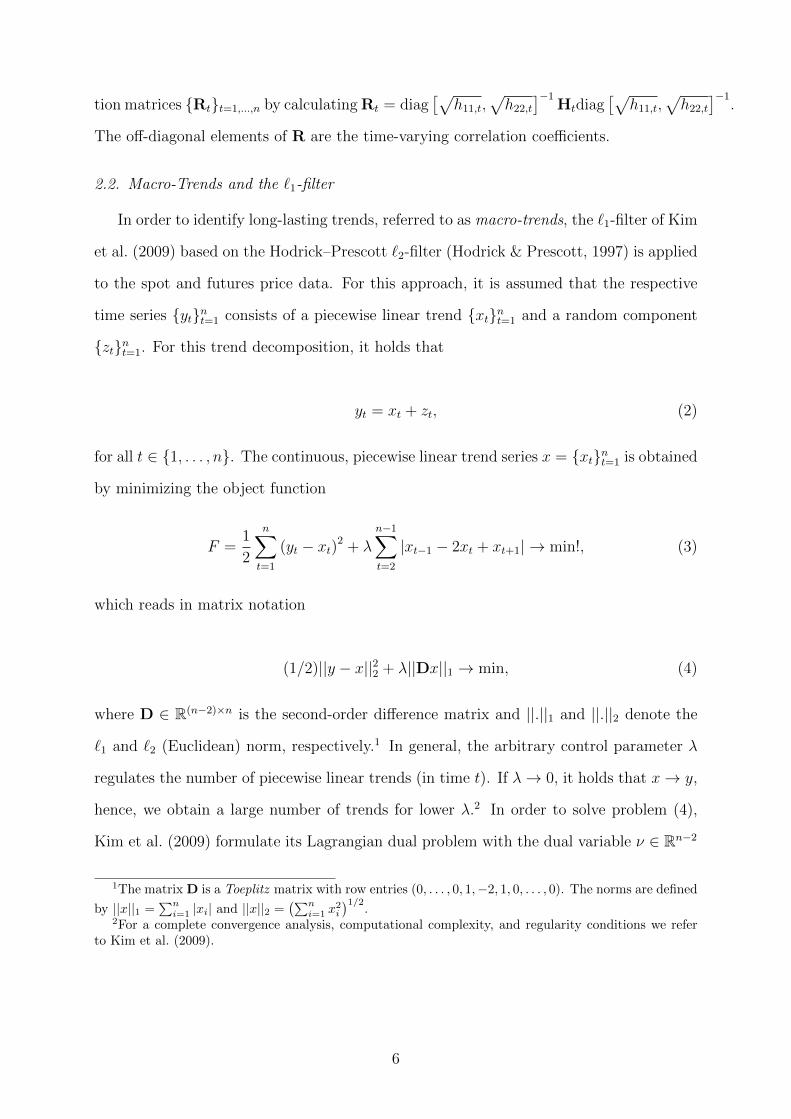
2.2. Macro-Trends and the `1-filter

In order to identify long-lasting trends, referred to as macro-trends, the `1-filter of Kim

et al. (2009) based on the Hodrick–Prescott `2-filter (Hodrick & Prescott, 1997) is applied

to the spot and futures price data. For this approach, it is assumed that the respective

time series ytnt=1 consists of a piecewise linear trend xtnt=1 and a random component

ztnt=1. For this trend decomposition, it holds that

yt = xt + zt, (2)

for all t ∈ 1, . . . , n. The continuous, piecewise linear trend series x = xtnt=1 is obtained

by minimizing the object function

F =1

2

n∑t=1

(yt − xt)2 + λn−1∑t=2

|xt−1 − 2xt + xt+1| → min!, (3)

which reads in matrix notation

(1/2)||y − x||22 + λ||Dx||1 → min, (4)

where D ∈ R(n−2)×n is the second-order difference matrix and ||.||1 and ||.||2 denote the

`1 and `2 (Euclidean) norm, respectively.1 In general, the arbitrary control parameter λ

regulates the number of piecewise linear trends (in time t). If λ→ 0, it holds that x→ y,

hence, we obtain a large number of trends for lower λ.2 In order to solve problem (4),

Kim et al. (2009) formulate its Lagrangian dual problem with the dual variable ν ∈ Rn−2

1The matrix D is a Toeplitz matrix with row entries (0, . . . , 0, 1,−2, 1, 0, . . . , 0). The norms are defined

by ||x||1 =∑n

i=1 |xi| and ||x||2 =(∑n

i=1 x2i

)1/2.

2For a complete convergence analysis, computational complexity, and regularity conditions we referto Kim et al. (2009).

6

(1/2)ν>DD>ν − y>Dν> → min!

s.t. − λ ≤ νi ≤ λ, ∀i = 1, . . . , n− 2.

(5)

The dual problem (5) is solved by interior-point methods, which is formulated in Kim

et al. (2009). The `1-trend estimate x∗ is obtained by a solution ν∗ of Eq. (5) and reads

x∗ = y −D>ν∗.

In applications, parameter choices for λ are dependent on the resolution of the data

and on the time series as well as the intended trend length. The parameter λ is not in a

linear relationship with the length and number of the obtained linear trends. In literature,

parameter choices and suggestions range from λ = 20 (Yamada & Yoon (2014) on roughly

110 years yearly data), λ = 100 (Kim et al. (2009) on five years of daily returns of the

S&P500), to λ = 1 000 up to λ = 10 000 for highly variable prices.3 As λ controls for

the number of trends, it naturally controls the number of breakpoints or, since the trend

is piecewise linear, kink points.4 Intuitively, when trying to model long-term trends, the

number of kink points should not be too high. We address this issue at a later point.

Assume that the number of trends is p. Similar as in Kim et al. (2009, p. 343), we

then split the observation times to a (unlikely equidistant) grid 1 = t1 < t2 < . . . < tp < n

obtained by the `1-filter. For all k = 1, . . . , p, it holds that

xt = αk + βkt, tk ≤ t ≤ tk+1, αk, βk ∈ R, (6)

which formalizes the piecewise linearity of the trends.5 Hence, we obtain p−1 kink points,

which are denoted by the set of dates

3Winkelried (2016) analyzes different choices of λ and presents an optimization approach for an optimalλ, depending on the desired path length.

4An increasing λ generally decreases the number of kink points. However, Kim et al. (2009) constructcounterexamples where this relationship does not hold. Hence, λ needs to be adjusted to the problemand data while λ’s for different time series are not comparable; see further Winkelried (2016).

5Note that the linearity in t does not hold for the widely-used `2 Hodrick-Prescott filter.

7

T× := t2, t3, . . . , tp.

We also define the transition set Λ := ∆t2 , . . . ,∆tp of cardinality p − 1, where for all

tk ∈ T×

∆tk :=

1, if (βk < 0) ∧ (βk+1 ≥ 0), or

−1, if (βk > 0) ∧ (βk+1 ≤ 0), or

0, else.

If we remove the dates ts from T× where ∆ts = 0, we obtain the set T×,str ⊂ T×, which

only contains kink points where a change of sign of the slope of the trend happens. Hence,

these dates are considered significant, since long-term trends change their direction.

In what follows, we interpret the piecewise linear `1-trends as long-term trends in

prices which are subject to interruption and change. We keep in mind that the exact kink

dates as well as their total number is dependent on the control variable λ in Eq. (3) and

the data. We fix λ = 2 000 and aim for trend lengths of several months. This is different

from previous applications of `1-trends where trends over decades are examined.6 The sets

T× and T×,str are used to compare break dates with event dates, such as OPEC meetings,

in order to evaluate the impact of these events on long-term trends. Two questions are

evaluated with `1-trends:

(Q1) Despite the existence of a varying spread, are the long-term trends of WTI and

Brent spot and futures price pairs driven by similar dynamics?

(Q2) Are OPEC conferences a major contributor to changes in these long-term trends?

2.3. Micro-Trends and Scoring

For trends in a short-term perspective, we implement an approach based on returns

and not prices as in the previous section. Given the log-returns of the WTI and Brent

6For robustness checks, we vary the choice of λ. An overview is given in the appendix. For T×,str,a threshold of 0.05 in absolute changes of β is implemented to filter for insignificant trends and theirchanges. I appreciate this suggestion made by one of the reviewers.

8

crude oil prices and their respective futures (see Section 3), we define the following trend

sets as subsets of the total daily observation dates T = 1, . . . , n:

T crude+,k :=

t : t− k + 1

∣∣∣∣rcrudet , rcrudet−1 , . . . , rcrudet−k+1 ≥ 0

and

T crude−,k :=

t : t− k + 1

∣∣∣∣rcrudet , rcrudet−1 , . . . , rcrudet−k+1 ≤ 0

.

(7)

The set T crude·,k contains all dates of positive or negative trends with a length of at least k

consecutive days. The price data is synchronized with a zero-order hold, hence returns

that are exactly equal to zero do not break a trend. Since trends which last longer than

k days are also elements of the respective k-sets, it holds that T crude·,m ⊂ T crude

·,k ⊂ T for

m > k. We then determine the intersection of the sets that describe dates where both

WTI and Brent are in the same type of trend simultaneously:

T∩+,k := TWTI+,k ∩ TBrent

+,k and

T∩−,k := TWTI−,k ∩ TBrent

−,k .

(8)

In order to determine information or price leading and lagging effects of one market to the

other, we intuitively define score functions which determine if a trend started earlier (and

lasted longer) than their respective counterpart. If this is the case, the score function is

increased by one for each day of leading a trend or lagging behind it.

If the magnitude of lead or lag is of interest, e.g. for how long is a trend active before

a contagion to the other market appears, the flexible score functions read:

SWTIlead,k,+,m,r =

∑t∈T∩+,k

r∑l=m

1TWTI+,k

(t− l)1TBrent+,k

(t− l),

SWTIlag,k,+,m,r =

∑t∈T∩+,k

r∑l=m

1TWTI+,k

(t+ l)1TBrent+,k

(t+ l),

(9)

where m determines the start and r determines the end of the period scored relative to

the beginning (for lead effects) or end (for lag effects) of the current trend. The score

9

function for Brent is defined analogously. For negative trends, the set T∩−,k is used. The

complement of a set is marked by the overline and refer to the sets defined in Eq. (7).7 If

m = r = 1, only the day before (for lead effects) and after (for lag effects) is checked and

scored. If m = 1 and r = 2, it is checked if the trend has been active for up to two days

before a translation happened.8

Examining micro-trends that represent under- and overreaction as well as some sort

of market sentiment, we focus on k = 3 and k = 5. The intuition of definition Eq. (9) is

as follows; when a trend in both return series is present, it is of some interest if there is a

contagion of this trend from one market into the other, or if the trends start at the same

time. The former case could be caused by events that influence local supply and demand

(e.g. storms or other infra-structure damage in one market, for a thorough discussion

see further: Kaufmann & Banerjee (2014)) and might also trigger a kink point in the `1

long-term trends. The latter case could be a reaction to a global shock, e.g. unexpected

OPEC decisions, which has been addressed by Schmidbauer & Rosch (2012) and Mensi

et al. (2014). The score function is used to answer the following questions:

(Q3) Is there an asymmetric transmission of micro-trends with respect to (1) the slope

of the trend as well as (2) contagion direction?

The sets defined in Eq. (7) and simultaneous trends in Eq. (8) are used to determine

triggers of short-term trends in order to answer:

(Q4) Do OPEC conferences trigger short-term trends and if so, is there a difference

between ordinary and extraordinary meetings?

2.4. Asymmetries in Variance

For the purpose of further understanding the relevance of micro-trends and connecting

the ideas and results of selected articles, we employ asymmetric conditional variance

models on daily returns of both crude oil spot and futures prices to answer the following

7Note that for Eq. (8) and Eq. (9), WTI and Brent are only placeholders for markets examined.Leading and lagging effects could also be examined in one market for futures of different maturities forexample.

8If m > 1, one has to ensure that the current trend has not been disrupted at m = 1. If it wasdisrupted, it does not count into the score function as there is no active trend.

10

question:

(Q5) Do short-term trends in returns have an asymmetric impact on the conditional

variance of WTI and Brent spot and futures prices?

For testing the hypothesis, we apply the APARCH model (Ding et al., 1993) and

FIAPARCH model (Tse, 1998) on AR(1)-filtered residuals with Student-t distributed

errors. The choice of this distribution is justified by the preliminary analysis of the return

data outlined in Section 3.

Let rt be the crude return series, our framework reads

rt = µ0 + µ1rt−1 + εt,

εt = zt√ht with zt ∼ St-t(ν) i.i.d.,

ht = Var (rt|Ft−1) ,

where the errors follow a standardized Students-t distribution. APARCH(1,1) is defined

as

hδ/2t = ω + α (|εt−1| − γεt−1)δ + βh

δ/2t−1,

and FIAPARCH(1,d,1) as

hδ/2t = ω +

(1− βL− (1− φL) (1− L)d

)(|εt| − γεt)δ + βh

δ/2t−1.

For non-negativity and stationarity conditions, we refer to the abundance of literature on

these models, e.g. Chkili et al. (2014) and Klein & Walther (2016) who include definitions,

estimation procedures, and application/comparison of these models to commodity and

crude oil markets.

We only take into consideration the estimated leverage parameters γ ∈ (−1, 1), the

11

long memory parameter d as well as power parameter δ > 1.9 The sign and magnitude

of the leverage parameter indicate whether positive or negative residuals influence the

conditional variance asymmetrically; and if so, to what extent. If the leverage parameter

γ is significantly different from zero, there is an asymmetric impact of positive and negative

residuals on the conditional variance. Hence, we would not reject the hypothesis. We also

compare the persistence of shocks in conditional variance with the fractional differencing

parameter d. In addition, we carry out a Likelihood Ratio test to determine if asymmetric

models offer a better fit than a symmetric GARCH:

LR = −2 (LLR − LLU) ,

where LLR refers to the log-likelihood of the restricted model (GARCH) and LLU to the

unrestricted models (APARCH and FIAPARCH, both nest the GARCH model). The test

statistic is asymptotically distributed as χ2, where the degree of freedom stems from the

difference of numbers of parameters used in the nesting models. The results are compared

with other studies of asymmetric impact of event-triggered shocks, e.g. Schmidbauer &

Rosch (2012), Mensi et al. (2014), and Loutia et al. (2016).

3. Data

Spot prices in US$/bbl are obtained from the U.S. Energy Information Administration

(EIA) from 01-Jan-2007 to 31-Mar-2017 as we want to focus on the most recent market

distortions. In order to synchronize trading days, a zero order hold (zoh) is established.

If a market is traded while the other is not, the non-traded market’s closing price is set

to the last closing price of the this market.10 Naturally, this produces returns equal to

zero, which is covered by the implementation of trend sets.

Futures prices in US$/bbl are obtained from Bloomberg from 01-Jan-2007 to 31-Mar-

9All other parameter estimates and robust standard errors are available upon request.10For example, this is the case for holidays, e.g. 04-Jul-2016 when Brent was traded and WTI was not.

Hence, the WTI closing price of Monday, 04-Jul-2016 is set to US$ 49.02, Friday’s closing price.

12

2017 for WTI (ticker CLx) and Brent (ticker COx) as daily prices of the generic next

month (CL1 and CO1), three months (CL3 and CO3), six months (CL6 and CO6),

and one year (CL12 and CO12) contracts. Again, these prices are zoh-synchronized in

accordance to the spot prices, yielding n = 2 595 observations for all time series. Spot

prices and their respective `1-trends are plotted in Fig. 2.

The chosen time frame covers 28 meetings of the OPEC conference. In what follows,

we distinguish between ordinary meetings, which are usually scheduled six months ahead,

and extraordinary meetings which are scheduled on short-notice and are usually reactions

to significant events or price shocks. An overview is given in Tab. 1. The combined, daily

output of the OPEC member states in million barrels per day is listed as an estimate

obtained from Bloomberg which is later compared to actual production targets (based on

the decision of the meeting, e.g. increase, maintain, or decrease/cut).

Date Meeting # Decision Type Output Date Meeting # Decision Type Output

15-Mar-2007 144 o Ord 30.1 11-Dec-2010 158 o Ext 29.111-Sep-2007 145 + Ord 31.3 09-Jun-2011 159 none Ord 29.305-Dec-2007 146 o Ext 31.7 14-Dec-2011 160 o Ord 30.501-Feb-2008 147 o Ext 32.2 14-Jun-2012 161 o Ord 31.505-Mar-2008 148 o Ord 32.4 12-Dec-2012 162 o Ord 31.009-Sep-2008 149 + Ord 32.6 31-May-2013 163 o Ord 30.524-Oct-2008 150 − Ext 32.1 04-Dec-2013 164 o Ord 29.717-Dec-2008 151 − Ext 29.6 11-Jun-2014 165 o Ord 29.815-Mar-2009 152 o Ord 27.7 27-Nov-2014 166 o Ord 30.928-May-2009 153 o Ext 28.2 05-Jun-2015 167 o Ord 31.310-Sep-2009 154 o Ord 28.4 04-Dec-2015 168 o Ord 32.022-Dec-2009 155 o Ext 29.0 02-Jun-2016 169 o Ord 32.517-Mar-2010 156 o Ord 29.2 28-Sep-2016 170 − Ext 33.914-Oct-2010 157 o Ord 29.1 30-Nov-2016 171 −/o Ord 34.1

Table 1: OPEC meetings, Output in mb/d, and decisions of production ceiling: increase (+), maintain(o), and decrease (−) in ordinary meetings (Ord) or extraordinary meetings (Ext). Meeting numbersattribute to OPEC press releases published on www.opec.org. Conference decisions on production levelsare referring to actual production levels at the time of the conference. Output estimates obtained fromBloomberg as Total OPEC Crude Oil Production Output Data which lists monthly estimates. Thenearest estimate to the OPEC conference date is listed.

Descriptive statistics and preliminary tests of returns of spot and selected futures

prices of WTI and Brent are presented in Tab. 2. The excess kurtosis is greater than zero,

suggesting a leptocurtic shape of the return distributions. Given the positive skewness

for spot prices, we find extreme positive returns to occur more often than their nega-

tive counterparts yielding a heavier right tail of the return distributions. For futures

returns, we observe a negative skewness. For all series, the augmented Dickey-Fuller

(ADF) test rejects the hypothesis of a unit root in the series which is in line with the

13

Kwiatkowski–Phillips–Schmidt–Shin (KPSS) test that does not reject the hypothesis of

stationarity of all series. The Ljung-Box test suggests a serial correlation of returns as

well as squared returns, which is a justification for the application of the conditional mean

and variance models described in Section 2.4. The Geweke & Porter-Hudak (GPH) es-

timator as well as the Detrended Fluctuation Analysis (DFA, Peng et al., 1994) reveal

long memory in squared returns of all series. This supports recent literature that finds

elevated shock persistence in variance of crude oils (Choi & Hammoudeh, 2009, Wang &

Wu, 2012, Chkili et al., 2014, Klein & Walther, 2016). Long memory in variance describes

the phenomenon that shocks (large returns, after AR(1) trend removal) of both positive

or negative sign cause an increase in variance which declines at a slow, hyperbolical rate.

WTI Brent CL1 CO1 CL3 CO3 CL6 CO6

n 2 595 2 595 2 595 2 595 2 595 2 595 2 595 2 595

Mean −0.0071 −0.0044 −0.0073 −0.0052 −0.0062 −0.0059 −0.0070 −0.0066Skewness 0.1576 0.1770 0.1693 −0.0170 −0.0546 −0.0167 −0.0778 −0.0316Kurtosis 7.4352 8.6438 7.5234 6.4435 5.9556 6.2858 6.0055 6.2141

ADF −52.28∗∗∗ −49.58∗∗∗ −53.95∗∗∗ −54.81∗∗∗ −54.44∗∗∗ −54.66∗∗∗ −55.95∗∗∗ −57.77∗∗∗KPSS 0.0459 0.0652 0.0455 0.0579 0.0474 0.0576 0.0458 0.0560

LB Q′(20) 55.42∗∗∗ 45.30∗∗∗ 42.75∗∗∗ 54.66∗∗∗ 48.17∗∗∗ 52.37∗∗∗ 46.57∗∗∗ 46.10∗∗∗

LB Q′2(20) 2649.50∗∗∗ 1235.48∗∗∗ 2652.20∗∗∗ 2623.13∗∗∗ 2116.66∗∗∗ 2136.16∗∗∗ 1801.29∗∗∗ 1810.88∗∗∗

GPH 0.3608 0.2130 0.2202 0.2455 0.2238 0.2372 0.2279 0.2387DFA 0.5554 0.5704 0.5653 0.5802 0.5616 0.5792 0.5595 0.5777

Note: Rejection of the respective hypothesis at 1% is market by ∗∗∗.

Table 2: Properties of the daily return series and test statistics of preliminary tests. Data for the 12months futures are available upon request.

4. Results & Discussion

4.1. Correlation Analysis within the BEKK Framework

In order to get a preliminary understanding on how WTI and Brent markets co-move,

we apply the BEKK model on zoh-synchronized spot returns of WTI and Brent. The

time-varying correlation is presented in Fig. 1. Unsurprisingly, the correlation is positive

throughout the data set. However, the BEKK model reveals a high variability in the

correlation coefficient. Even if smoothed by an MA(50) filter (red line), a strong seasonal

component seems present, especially between 2010 and 2015. On average, the coefficient

takes values around 0.6 with recurring spikes as high as 0.8-0.9 and as low as 0.2. The

14

oil price shock in 2008/2009 led to a complete temporal decoupling of price movements

and the correlation dropped as low as 0 for a few trading days. This decoupling effect

is found in earlier time periods in Maslyuk & Smyth (2009) and Fattouh (2010). Two

other lows can be found late 2014 and early 2015 as well as in the beginning of the

sample. These phenomenons are short-lived, however, since the smoothing does not drop

as low. Recently in 2016/2017, we observe a stronger coupling of returns with correlation

and smoothing reaching highs around 0.8. The correlation of the respective futures pairs

reveal similar properties and patterns. Unsurprisingly, the correlation of the spot prices

with futures prices is very high and close to one. Only in extreme downward movements

as in mid-2008 and mid-2014, the correlation drops shortly as the futures prices react

with some delay and the price deterioration is less abrupt.

Notably between 2009 and 2017, almost all OPEC meetings (see Tab. 1) lead to an

increase in correlation between WTI and Brent returns, at least on a daily base (blue

line). Oftentimes, this increase is jump-like. An example is OPEC meeting #168 on

04-Dec-2015. During the following trading days, the conditional correlation jumps from

0.35 to 0.65 within a few days and later to 0.85.

2007 2008 2009 2010 2011 2012 2013 2014 2015 2016 2017

Time

-0.1

0

0.1

0.2

0.3

0.4

0.5

0.6

0.7

0.8

0.9

Co

rre

latio

n C

oe

ffic

ien

t ρ

Figure 1: Correlation coefficient of WTI and Brent returns between 02-Jan-2007 to 31-Mar-2017, esti-mated with the fully parameterized BEKK framework (blue) and MA(50) smoothing (red).

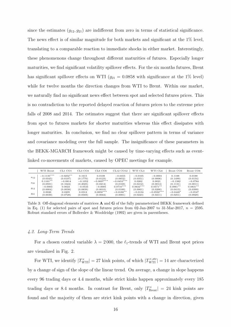
Tab. 3 reports the off-diagonal elements of the matrices A and G which depict a news

and a contagion or spillover effect, respectively. For the spot market, we find a significant

cross-market news effect from the estimates (a12, a21) but no general volatility spillover

15

since the estimates (g12, g21) are indifferent from zero in terms of statistical significance.

The news effect is of similar magnitude for both markets and significant at the 1% level,

translating to a comparable reaction to immediate shocks in either market. Interestingly,

these phenomenons change throughout different maturities of futures. Especially longer

maturities, we find significant volatility spillover effects. For the six months futures, Brent

has significant spillover effects on WTI (g21 = 0.0858 with significance at the 1% level)

while for twelve months the direction changes from WTI to Brent. Within one market,

we naturally find no significant news effect between spot and selected futures prices. This

is no contradiction to the reported delayed reaction of futures prices to the extreme price

falls of 2008 and 2014. The estimates suggest that there are significant spillover effects

from spot to futures markets for shorter maturities whereas this effect dissipates with

longer maturities. In conclusion, we find no clear spillover pattern in terms of variance

and covariance modeling over the full sample. The insignificance of these parameters in

the BEKK-MGARCH framework might be caused by time-varying effects such as event-

linked co-movements of markets, caused by OPEC meetings for example.

WTI Brent CL1 CO1 CL3 CO3 CL6 CO6 CL12 CO12 WTI CL3 WTI CL6 Brent CO3 Brent CO6

a12−0.1135∗∗∗ −0.0252∗∗ 0.1615 0.0108 −0.0455 −0.0105 −0.0004 0.1188 0.0188(0.0345) (0.0107) (0.1770) (0.0123) (0.0652) (0.0351) (0.0006) (0.1499) (0.0134)

a210.1161∗∗ −0.0814 −0.1052 −0.0697∗∗∗ −0.0453∗∗∗ 0.0262 0.0021 −0.1382 −0.0784(0.0591) (0.1624) (0.2025) (0.0214) (0.0169) (0.0412) (0.0014) (0.1131) (0.0811)

g12−0.0003 0.0022 −0.0533 −0.0005 0.0710∗∗∗ 0.0632∗∗∗ 0.0571∗∗ 0.0961∗∗ 0.0831∗∗

(0.0004) (0.0038) (0.0839) (0.0010) (0.0189) (0.0061) (0.0266) (0.0413) (0.0399)

g210.0026 0.0205 0.0312 0.0858∗∗∗ −0.0188∗∗ −0.0134 −0.0592∗∗∗ −0.0448∗ −0.0547(0.0039) (0.0728) (0.0569) (0.0044) (0.0081) (0.0223) (0.0211) (0.0251) (0.0929)

Table 3: Off-diagonal elements of matrices A and G of the fully parameterized BEKK framework definedin Eq. (1) for selected pairs of spot and futures prices from 02-Jan-2007 to 31-Mar-2017, n = 2595.Robust standard errors of Bollerslev & Wooldridge (1992) are given in parentheses.

4.2. Long-Term Trends

For a chosen control variable λ = 2 000, the `1-trends of WTI and Brent spot prices

are visualized in Fig. 2.

For WTI, we identify |T×WTI| = 27 kink points, of which |T×,strWTI | = 14 are characterized

by a change of sign of the slope of the linear trend. On average, a change in slope happens

every 96 trading days or 4.4 months, while strict kinks happen approximately every 185

trading days or 8.4 months. In contrast for Brent, only |T×Brent| = 24 kink points are

found and the majority of them are strict kink points with a change in direction, given

16

2007 2008 2009 2010 2011 2012 2013 2014 2015 2016 2017

Time

20

40

60

80

100

120

140

160

Price

in

US

D/b

bl

WTI Spot

Brent Spot

WTI l1 Trend

Brent l1 Trend

#145 #150 #155 #160 #165 #170

Figure 2: Spot prices of WTI and Brent crude oil and their respective `1-trends (λ = 2 000) from 01-Jan-2007 to 31-Mar-2017. The dates of OPEC meetings are visualized by black vertical lines. The numbersrefer to the meeting numbers. See also Tab. 1.

by |T×,strBrent| = 16. This yields an average length of trends of 108 days or 4.9 months and

strict kinks happen every 162 trading days or 7.4 months.

Notably, almost all strict kink points (changes in direction) of the long term trends are

identical for WTI and Brent spot prices in a time window of up to three trading days. This

is of particular interest as it shows that long term trends for WTI and Brent are variable

(any change of slope, denoted by the kink points T×), but major long term trend changes

(strict kink points) are identified to happen at identical times in both markets. Despite

varying slope of the trends, mainly between 2011 and mid-2014, these findings are in favor

to the one great pool hypothesis, which also partially answers our first question about

similar long-term price dynamics. Both markets share similar break points and the general

price direction is identical in most long-term trends. In addition, the long-term trends are

very close and almost indistinguishable from 2007 to the end of 2010 and from mid-2014

to the end of the observation in March 2017, despite the existence of elevated spreads

during these times. By means of the `1-filter, the linear trend components (x = xtnt=1 in

Eq. (2)) for WTI and Brent are driven by the same long-term process while the stochastic

component (z = ztnt=1) accounts for the variation in the spread, which is in line with

findings regarding cointegration of these markets. These results remain intact for other

17

choices of λ.11 If xWTI, the long-term trend component in the WTI prices, is regressed

against xBrent (and vice versa) by

xBrentt = β0 + β1x

WTIt + εt,

we obtain an explanatory power of R2 = 0.936. The vast majority of variation in the

long-term trends of one market is explained by the other crude’s long-term trend. This

is evidence that spot prices share the same underlying long-term trend which answers

our first question. For futures price pairs, the difference in long-term trends becomes less

pronounced, the coefficient of determination increases to R2 = 0.941 (CL1/CO1 pair),

R2 = 0.951 (CL3/CO3), and R2 = 0.958 (CL6/CO6 and CL12/CO12 pair). We infer

that the market assumes a long-term equilibrium of the WTI and Brent or, at least, a

convergence of spreads towards zero.

In order to understand OPEC’s effect on long-term trends, we examine T×WTI, T×,strWTI ,

and their respective counterparts for Brent. Obviously, not all OPEC meetings have

immediate impact on long-term trends as well as the spread of WTI and Brent within a

pre-defined announcement window. We fix λ = 2 000.12 If all OPEC meetings are taken

into consideration, only 5 of 14 (5 of 27) strict (soft) long-trend changes are triggered

within five trading days of the meeting for WTI. For Brent, 2 of 16 (2 of 24) strict (soft)

trend changes are triggered immediately after OPEC meetings. If we expand the time

window to one month (22 trading days) prior and after the meeting, 6 of 14 (11 of 27) for

WTI and for Brent 7 of 16 (13 of 24) strict (soft) trend changes are triggered by OPEC

meetings. We follow that OPEC meetings are not the main driver of strict changes in

long-term trends of crude oil prices which answers our second question. Similar results are

obtained for all futures prices and detailed results for three-months futures are reported

in Appendix Tab. 8. We also find no evidence that the current price level (as in Loutia

et al. (2016)) or the timing (during positive or negative long term trends) influences the

11With increasing λ, the portion of strict kink points out of all kink points is increasing while the totalnumber of kinks is decreasing.

12The following results are also available for different realizations of λ in Appendix Tab. 7.

18

impact of OPEC decisions on `1-trends. Between 2009 and 2016, all OPEC meetings

concluded in a ‘maintain’ decision (up to meeting #169) and no immediate action seems

to be taken by producing countries. Hence, market expectations which are not met by

the decisions could lead to price reactions (Schmidbauer & Rosch, 2012). This is also

addressed in the next section. The actual output of OPEC countries varies, however,

despite a theoretical ‘maintain’ regime. This becomes obvious from the last column in

Tab. 1.13 Also, production behavior in times of market shocks differs. The output strongly

declined during the shock in 2009, from 32.6mb/d in September 2008 to 27.7mb/d in

March 2009. During the decline in 2014, oil production was significantly increased on

the other hand from merely 29.8mb/d in June 2014 at prices around US$110 per barrel

to 32.5mb/d in June 2016 at prices around US$50 per barrel. This could be one of the

reasons why OPEC meetings do not play a significant role in long-term trends, given

that decisions seem to be not-binding for the respective member states. A cut decision

happens in the 170th, extraordinary meeting also labeled ‘Algiers Accord’ with an OPEC-

14 production target at 32.5mb/d. This decision is prolonged in the 171th meeting despite

rising production levels of the member states. Both meetings have no immediate impact

on the current, upward directed trend.

From the long-term perspective, we now move on to short-term trends, their reaction

to OPEC meetings, and how these trends move between markets. This introduces some

time-variability to contagion effects as we identify only weak effects for the full period of

daily prices and returns.

4.3. Short-term trends in AR(1)-filtered returns

The total number of positive micro-trends for k = 3 and k = 5 trading days obtained

with the score functions defined in Eq. (9) is presented in Tab. 4. As expected, the

number of short-term trends of the WTI and Brent markets as well as spot and different

futures maturities is similar. Also the total number of positive and negative trends are

roughly the same for each pair.

13For example, the actual output of OPEC countries increased from 27.7mb/d in March 2009 to31.5mb/d in June 2012, despite ‘maintain’ decisions.

19

WTI Spot Brent Spot WTI CL1 Brent CO1k positive negative positive negative positive negative positive negative

3 162 163 166 162 160 166 144 1565 42 45 49 43 38 40 33 39

WTI CL3 Brent CO3 WTI CL6 Brent CO6k positive negative positive negative positive negative positive negative

3 156 162 145 154 159 157 137 1515 39 37 36 38 41 35 41 37

Table 4: Number of trends of length k = 3 and k = 5 days. The results for the twelve month futures areavailable upon request.

Spillover and leading/lagging effects of trends in return data are examined with the

score functions defined in Eq. (9). Results for spot, one, and twelve months futures

are given in Tab. 5 for trends which are active—for at least one day simultaneously—in

both markets (all days in T∩+,k and T∩−,k). For k = 3, we distinguish between trends of

positive and negative direction. Leading effects in positive trends of spot prices cannot be

identified, trends in WTI start earlier only slightly more often. With increasing maturity

of futures, we observe a leading effect for WTI over Brent. A prominent lagging effect

of positive trends in Brent is obvious which is of particular strength in futures of longer

maturity. Trends stay intact for one or two days longer (absolute scores WTI: 39 to Brent:

74) while WTI has already terminated the current micro-trend. The same effect is present

in futures markets. For negative 3-day trends, WTI leads over Brent (58 to 36), causing

a consistent lagging effect in Brent (32 to 48). Negative trends start in WTI markets

and with some delay, Brent markets enter the same trend which even lasts when WTI

markets turned to positive returns. This phenomenon is visible in futures prices. For

twelve months futures, this lagging effect is more pronounced. For longer trends tested

with k = 5, the results are even clearer. The number of overlapping trends is reduced,

however (see also Tab. 4). Positive trends of WTI are transferred to Brent markets with

some delay while Brent clearly lags behind (lead 10 to 5 and lag 6 to 15). The picture

becomes more significant if negative trends are taken into consideration. The majority of

negative trends starts in WTI markets (score: 16 to 4) while Brent outlasts with a clear

lagging structure (score: 5 to 18). We observe similar behavior for futures. In view of

our third question, (Q3), we find that there is a significant contagion of negative trends

from WTI to Brent markets. This leading effect in positive trends is also present but not

20

as strong. This is in line of findings of Elder et al. (2014) and identifies asymmetries. In

addition, we identify a strong lagging of Brent markets relative to trends in WTI markets.

Scrude,k,trend,m,r lead lag lead lag lead lag

k trend m r WTI Brent WTI Brent CL1 CO1 CL1 CO1 CL12 CO12 CL12 CO12

3 + 1 1 38 27 25 51 14 13 12 21 44 10 15 463 + 1 2 56 43 39 74 18 19 13 30 47 18 31 51

3 − 1 1 41 24 24 34 16 17 16 21 43 17 6 503 − 1 2 58 36 32 48 23 25 21 32 50 31 16 62

5 + 1 1 5 3 3 9 4 0 4 6 13 2 4 125 + 1 2 8 4 5 13 6 0 5 9 13 4 7 135 + 1 3 10 5 6 15 6 0 6 9 13 6 10 14

5 − 1 1 9 2 5 8 5 4 4 5 5 5 3 65 − 1 2 15 3 5 14 9 7 6 8 7 8 5 95 − 1 3 16 4 5 18 10 8 7 11 7 9 6 10

Table 5: Results of the score function defined in Eq. (9). Results for futures prices of the remainingmaturities are available upon request.

We revisit the sets T∩+,k and T∩−,k and check if OPEC meeting days are elements of these

trend sets. In our time period, 28 OPEC meetings are included (see Tab. 1) of which eight

are extraordinary conferences. For WTI, 16 (8) micro-trends of three (five) day length are

triggered immediately after the meeting day. If we check for the following week of trading,

this number increases to 23 (11) triggered trends. For Brent, these number are higher.

Immediately after OPEC meetings, 21 (9) three (five) day trends in Brent returns start.

Within a trading week, 26 (13) trends are initiated. If we only consider eight extraordinary

meetings, 6 (4) three (five) day trends in WTI are triggered. For Brent, all meetings cause

a three day trend and six an even longer trend of five days. We note that OPEC meetings

cause more trends in Brent returns than in WTI returns. Also, if we allow the market

to react to the results of the meeting within a week, almost all meetings cause short-

term trends in both WTI and Brent spot markets, which positively answers both parts

of our fourth question, Q4; the majority of OPEC meetings triggers short-term trends

whereas all extraordinary meetings cause trends in Brent. These results are comparable

with findings of Mensi et al. (2014). Notably, approximately 75% of triggered trends in

WTI are positive while this ratio is reduced to two thirds in Brent. Implications of these

findings are manifold. We find that the Brent spot and futures prices are more sensitive

to OPEC decisions which might be due to the regional proximity to major producers

of the OPEC. Extraordinary meetings play a significant role as all of them trigger a

21

trend. On the other side, OPEC decisions are slightly less important in WTI markets.

From the leading/lagging relationship, it appears that WTI dominates Brent prices and

volatility as a benchmark, particularly in negative price movements and Brent follows

with lags of several days. With the correlation results, these directional spillover effects

are of temporary nature. This asymmetry is further examined in the next subsection.

The implications of these findings are important as they indicate that Brent markets

could appear robust to WTI price shocks but follow a negative trend with some delay

nonetheless. Here, it is shown that OPEC announcements trigger such trends. Other

events, such as storage publications, could also serve as trigger events which ultimately

spill over to other markets.

4.4. Asymmetries in volatility and the impact of short-term trends

Tab. 6 presents relevant parameters of asymmetric and long memory variance models.

Firstly, leverage parameters are statistically significant and high compared to other asset

classes.14 For WTI and its futures prices, the leverage parameter γ of APARCH ranges

between 0.5878 for spot and declines to 0.3192 for the 12M futures prices. Additionally

accounting for long memory effects in the FIAPARCH framework reduces the leverage

parameters to more moderate levels. For Brent, parameter levels are slightly lower in

APARCH whereas we observe further reduction throughout futures maturities. It also

holds that asymmetry parameters are decreasing in the FIAPARCH model. Secondly,

all leverage parameter estimates are positive. This translates to an increase of volatility

if residuals (AR-filtered returns) are negative. Given the magnitude of γ, the volatility

strongly reacts to negative residuals. This behavior is additionally amplified during ongo-

ing negative trends. Lastly, these effects are reduced in futures markets. Both WTI and

Brent futures prices feature less asymmetric response to negative shocks to their variance

with longer maturity. This is in line with our findings from the fully parameterized BEKK

and estimates given in Tab. 3. The variance of futures has a less pronounced asymmetric

news impact and there is no significant news impact between the markets whereas we

14An overview of estimations for different commodities can be found Chkili et al. (2014), for example.

22

observe spillovers from the spot to futures markets. The persistence of variance shocks

measured by d in FIAPARCH and in parts by δ in APARCH (Ding et al., 1993) remains

stable throughout all contract maturities.

Compared to literature which applies identical models to crude oil prices (e.g. Chkili

et al., 2014, Klein & Walther, 2016), the focus on a smaller yet more volatile time pe-

riod reveals some interesting volatility properties. Especially the APARCH asymmetry

parameter γ is higher while shock persistence, depicted by d in FIAPARCH, is reduced

compared to empirical findings for longer time horizons. These findings seem reasonable

considering two extreme price shocks and strong upward movements happened during the

examined, shorter period in the present paper.15

In conclusion, asymmetry parameters for the variance of crude spot and futures returns

are statistically significant throughout all tested series. The likelihood-ratio test rejects

the GARCH model (null hypothesis) in favor to unrestricted models. This holds for both

APARCH and FIAPARCH. Loglikelihood (LL) and BIC are in favor to models which

include asymmetric news impact and long memory. We observe that long memory models

seem to provide a better fit for longer maturity of futures prices whereas APARCH is the

outperforming model for spot returns and futures of shorter maturities.

Transferring these findings to the existence of micro-trends of variable length outlined

in the previous session, negative trends lead to a strong increase in conditional volatility.

In addition, there is a spillover effect in variance given the identified transmission of micro-

trends from one market to another. By means of the Bayesian information criterion and

a Likelihood ratio test (results in Tab. 6), we find some degree of persistence and—more

importantly—strong asymmetric effects. These effects are amplified in negative trends.

Positive short term trends are of lesser impact to variance and we can therefore answer

the fifth assertion, Q5. Considering the identified lagging behavior of Brent, for negative

trends in particular, we infer that also the conditional variance stays elevated longer those

temporal trend situations.

15The estimations are repeated on a rolling window of length n = 1 000. The interpretations of theparameter estimates remain qualitatively the same, albeit now of a time-varying nature.

23

WTI Brent CL1 CO1 CL3 CO3 CL6 CO6 CL12 CO12

APARCHγ

0.5878 0.4631 0.5429 0.3890 0.4566 0.3779 0.4114 0.3332 0.3192 0.2635(0.1611) (0.1317) (0.1467) (0.1624) (0.1347) (0.1371) (0.1298) (0.1338) (0.1382) (0.1351)

δ1.2619 1.7506 1.3805 1.5546 1.4607 1.5588 1.4665 1.5881 1.5831 1.6677(0.3269) (0.3330) (0.2903) (0.4266) (0.3243) (0.4147) (0.3925) (0.4264) (0.5011) (0.5138)

LL −5 524.3 −5 265.6 −5 509.2 −5 285.7 −5 313.1 −5 154.6 −5 096.4 −4 983.0 −4 760.5 −4 697.6BIC 11 111 10 594 11 081 10 634 10 689 10 373 10 256 10 029 9 583 9 460

FIAPARCH

γ0.3127 0.2782 0.2850 0.2317 0.2642 0.2141 0.2422 0.2051 0.1908 0.1827(0.0595) (0.0758) (0.0934) (0.0794) (0.0757) (0.0892) (0.0815) (0.0984) (0.0667) (0.0746)

δ1.6945 2.1380 1.8312 1.9956 1.9499 2.0368 1.9960 2.0652 2.1105 2.1061(0.1460) (0.1631) (0.2527) (0.2053) (0.2045) (0.3563) (0.2549) (0.2537) (0.3056) (0.3112)

d0.4917 0.3369 0.4385 0.4120 0.4063 0.3864 0.3899 0.3701 0.3740 0.3634(0.1679) (0.0933) (0.1872) (0.0959) (0.1157) (0.1639) (0.1250) (0.1518) (0.1969) (0.1782)

LL −5 530.6 −5 275.3 −5 513.0 −5 286.4 −5 315.6 −5 151.3 −5 096.1 −4 981.1 −4 756.5 −4 693.4BIC 11 132 10 621 11 097 10 644 10 702 10 373 10 263 10 033 9 583 9 457

GARCH LL −5 554.2 −5 281.7 −5 541.1 −5 304.4 −5 338.3 −5 176.6 −5 120.1 −5 004.0 −4 782.1 −4 717.1BIC 11 156 10 611 11 129 10 656 10 724 10 400 10 287 10 055 9 611 9 481

Table 6: Asymmetric properties of the conditional variance of the return series (n = 2 595) of WTIand Brent spot and selected futures prices from 01-Jan-2007 to 31-Mar-2017. Models refer to theAPARCH(1,1), FIAPARCH(1,1) and GARCH(1,1) frameworks with an AR(1) conditional mean structureand Student’s-t distributed errors. Log-likelihoods in bold font mark the rejection of the null hypothesisat 1% in a Likelihood-Ratio test (null: GARCH model). Underlined BIC values refer to the best fit. Theremaining parameters and their robust standard errors of the estimates are available upon request.

5. Conclusion

In this paper, the interconnectedness of WTI and Brent spot and futures markets is

revisited with recent data between 2007 and 2017. Within a fully parameterized BEKK

framework, we observe high correlations of prices that average around 0.6. The correlation

is volatile with spikes of 0.9 and drops as low as 0. We find OPEC meetings to increase the

correlation on the short-run. In 2016, the correlation of spot prices moves to relatively high

levels where it remains. These findings are of importance to hedging strategies, as higher

correlations reduce the hedging potential between these crude markets, in particular for

futures. For spot prices, we identify a significant news effect between the markets but no

general volatility spillover over the full sample, highlighting the possibility of time-varying

contagion. For futures of longer maturities, contagion effects are present.

With the recently introduced `1-trends, we obtain long-term trends that change direc-

tion every 8.4 months for WTI and 7.4 months for Brent. We find that these long-term

trends are driven by very similar dynamics. In addition, an increasing explanatory power

in futures markets is observed. This is in favor of the globalized market or ‘one great

pool’ hypothesis. These long term trends offer more insight on the explanation of the

WTI-Brent spread and suggest a reversal to a long-run equilibrium. Some of the occur-

ring trend reversals fall together with OPEC meetings (e.g. #160, #161, and #165),

24

however, there is no general tendency or evidence that OPEC meetings have significant

influence on long-term trends in crude oil prices.

In an analysis of micro-trends in returns, we find significant leading effects of WTI

relative to Brent for both positive and negative short-term trends of several days. Brent

depicts lagging behavior. In addition, these trends have an asymmetrical impact on

volatility of these crudes. Negative trends lead to a significantly higher volatility than

positive trends. Hence, we infer temporal spillover effects from WTI to Brent, in particular

for negative trends. Almost all OPEC meetings trigger short-term trends. Their direction,

however, cannot be explained by decision or current price level. We assume that these

trends account for a possible mismatch of expected decisions.

The application of `1-trends to oil prices carries some potential for further research.

For example, the estimated change points of the `1-trend could be used to build a causality

test between OPEC decisions and current price and slope level. This might offer additional

insight on what drives and influences OPEC decisions. Also, `1-trends could be applied

to calculate excess movements of prices from its current trend in order to identify shocks

or jumps.

25

6. Appendix

To be made available as supplementary material.

λBrent 2 000 4 000 10 000

±T

5 (7) 2 of 16 (2 of 24) 2 of 12 (2 of 17) 1 of 5 (1 of 11)22 (30) 7 of 16 (13 of 24) 6 of 12 (9 of 17) 2 of 5 (5 of 11)44 (60) 12 of 16 (20 of 24) 10 of 12 (14 of 17) 4 of 5 (10 of 11)66 (90) 15 of 16 (23 of 24) 12 of 12 (17 of 17) 5 of 5 (11 of 11)

WTI 2 000 4 000 10 000

±T

5 (7) 5 of 14 (5 of 27) 2 of 14 (3 of 20) 0 of 7 (1 of 11)22 (30) 6 of 14 (11 of 27) 6 of 14 (8 of 20) 1 of 7 (2 of 11)44 (60) 10 of 14 (20 of 27) 10 of 14 (15 of 20) 5 of 7 (9 of 11)66 (90) 14 of 14 (27 of 27) 14 of 14 (20 of 20) 7 of 7 (11 of 11)

Table 7: WTI and Brent Spot prices: Absolute numbers of strict trend changes (all trend changes)explained by OPEC meetings in a given time window of ±T trading days (calender days in parentheses)from the change date.

λCO3 2 000 4 000 10 000

±T

5 (7) 0 of 15 (2 of 24) 2 of 12 (2 of 18) 1 of 5 (2 of 9)22 (30) 6 of 15 (13 of 24) 5 of 12 (7 of 18) 2 of 5 (3 of 9)44 (60) 11 of 15 (19 of 24) 9 of 12 (14 of 18) 4 of 5 (8 of 9)66 (90) 15 of 15 (24 of 24) 12 of 12 (18 of 18) 5 of 5 (9 of 9)

CL3 2 000 4 000 10 000

±T

5 (7) 1 of 14 (3 of 25) 1 of 11 (2 of 17) 0 of 8 (1 of 13)22 (30) 6 of 14 (12 of 25) 3 of 11 (5 of 17) 2 of 8 (3 of 13)44 (60) 10 of 14 (19 of 25) 7 of 11 (12 of 17) 4 of 8 (9 of 13)66 (90) 14 of 14 (25 of 25) 11 of 11 (17 of 17) 8 of 8 (13 of 13)

Table 8: WTI and Brent three months futures prices: Absolute numbers of strict trend changes (all trendchanges) explained by OPEC meetings in a given time window of ±T trading days (calender days inparentheses) from the change date.

26

Bibliography

Bollerslev, T. (1986). Generalized autoregressive conditional heteroskedasticity. Journalof Econometrics , 31 , 307–327. doi:10.1016/0304-4076(86)90063-1.

Bollerslev, T., & Wooldridge, J. M. (1992). Quasi-maximum likelihood estimation andinference in dynamic models with time-varying covariances. Econometric Reviews , 11 ,143–172. doi:10.1080/07474939208800229.

Caporin, M., & McAleer, M. (2013). Ten Things You Should Know about the Dy-namic Conditional Correlation Representation. Econometrics , 1 , 115–126. doi:10.3390/econometrics1010115.

Chen, H., Liao, H., Tang, B.-J., & Wei, Y.-M. (2016). Impacts of OPEC’s political riskon the international crude oil prices: An empirical analysis based on the SVAR models.Energy Economics , 57 , 42–49. doi:10.1016/j.eneco.2016.04.018.

Chkili, W., Hammoudeh, S., & Nguyen, D. K. (2014). Volatility forecasting and riskmanagement for commodity markets in the presence of asymmetry and long memory.Energy Economics , 41 , 1–18. doi:10.1016/j.eneco.2013.10.011.

Choi, K., & Hammoudeh, S. (2009). Long memory in oil and refined products markets.Energy Journal , 30 , 97–116. doi:10.5547/ISSN0195-6574-EJ-Vol30-No2-5.

Ding, Z., Granger, C. W. J., & Engle, R. F. (1993). A long memory property of stockmarket returns and a new model. Journal of Empirical Finance, 1 , 83–106.

Elder, J., Miao, H., & Ramchander, S. (2014). Price discovery in crude oil futures. EnergyEconomics , 46 , 18–27. doi:10.1016/j.eneco.2014.09.012.

Engle, R. (2002). Dynamic Conditional Correlation. Journal of Business & EconomicStatistics , 20 , 339–350. doi:10.1198/073500102288618487.

Engle, R. F., & Kroner, K. F. (1995). Multivariate Simultaneous Generalized ARCH.Econometric Theory , 11 , 122–150. doi:10.1017/S0266466600009063.

Fattouh, B. (2010). The dynamics of crude oil price differentials. Energy Economics , 32 ,334–342. doi:10.1016/j.eneco.2009.06.007.

Hamilton, J. D. (2017). Why You Should Never Use the Hodrick-Prescott Filter. TheReview of Economics and Statistics , Forthc., 1–45. doi:10.1162/REST\_a\_00706.

Hodrick, R. J., & Prescott, E. C. (1997). Postwar U.S. Business Cycles: An EmpiricalInvestigation. Journal of Money, Credit and Banking , 29 , 1. doi:10.2307/2953682.

Ji, Q., & Fan, Y. (2015). Dynamic integration of world oil prices: A reinvestigationof globalisation vs. regionalisation. Applied Energy , 155 , 171–180. doi:10.1016/j.apenergy.2015.05.117.

Kaufmann, R. K., & Banerjee, S. (2014). A unified world oil market: Regions in physical,economic, geographic, and political space. Energy Policy , 74 , 235–242. doi:10.1016/j.enpol.2014.08.028.

27

Kaufmann, R. K., Dees, S., Karadeloglou, P., & Sanchez, M. (2004). Does OPEC mat-ter? an econometric analysis of oil prices. Energy Journal , 25 , 67–90. doi:10.5547/ISSN0195-6574-EJ-Vol25-No4-4.

Kim, B.-H., Kim, H., & Lee, B.-S. (2015). Spillover effects of the U.S. financial crisis onfinancial markets in emerging Asian countries. International Review of Economics &Finance, 39 , 192–210. doi:10.1016/j.iref.2015.04.005.

Kim, S.-J., Koh, K., Boyd, S., & Gorinevsky, D. (2009). l1 Trend Filtering. SIAM Review ,51 , 339–360. doi:10.1137/070690274.

Klein, T., & Walther, T. (2016). Oil Price Volatility Forecast with Mixture MemoryGARCH. Energy Economics , 58 , 46–58. doi:10.1016/j.eneco.2016.06.004.

Loutia, A., Mellios, C., & Andriosopoulos, K. (2016). Do OPEC announcements influenceoil prices? Energy Policy , 90 , 262–272. doi:10.1016/j.enpol.2015.11.025.

Maslyuk, S., & Smyth, R. (2009). Cointegration between oil spot and future prices ofthe same and different grades in the presence of structural change. Energy Policy , 37 ,1687–1693. doi:10.1016/j.enpol.2009.01.013.

Mensi, W., Hammoudeh, S., & Yoon, S. M. (2014). How do OPEC news and structuralbreaks impact returns and volatility in crude oil markets? Further evidence from a longmemory process. Energy Economics , 42 , 343–354. doi:10.1016/j.eneco.2013.11.005.

Nomikos, N. K., & Pouliasis, P. K. (2011). Forecasting petroleum futures markets volatil-ity: The role of regimes and market conditions. Energy Economics , 33 , 321–337.doi:10.1016/j.eneco.2010.11.013.

Peng, C. K., Buldyrev, S. V., Havlin, S., Simons, M., Stanley, H. E., & Goldberger, A. L.(1994). Mosaic organization of DNA nucleotides. Physical Review E , 49 , 1685–1689.doi:10.1103/PhysRevE.49.1685.

Pindyck, R. S. (1999). The Long-Run Evolutions of Energy Prices. The Energy Journal ,20 , 1–28. doi:10.5547/ISSN0195-6574-EJ-Vol20-No2-1.

Reboredo, J. C. (2011). How do crude oil prices co-move ? A copula approach. EnergyEconomics , 33 , 948–955. doi:10.1016/j.eneco.2011.04.006.

Schmidbauer, H., & Rosch, A. (2012). OPEC news announcements: Effects on oil priceexpectation and volatility. Energy Economics , 34 , 1656–1663. doi:10.1016/j.eneco.2012.01.006.

Tse, Y. K. (1998). The conditional heteroscedasticity of the yen-dollar exchange rate.Journal of Applied Econometrics , 13 , 49–55. doi:10.1002/(SICI)1099-1255(199801/02)13:1<49::AID-JAE459>3.0.CO;2-O.

Wang, Y., & Wu, C. (2012). Forecasting energy market volatility using GARCH models:Can multivariate models beat univariate models? Energy Economics , 34 , 2167–2181.doi:10.1016/j.eneco.2012.03.010.

Weiner, R. J. (1991). Is the world oil market ‘one great pool’?. Energy Journal , 12 ,95–107. doi:10.5547/ISSN0195-6574-EJ-Vol12-No3-7.

28

Winkelried, D. (2016). Piecewise linear trends and cycles in primary commodity prices.Journal of International Money and Finance, 64 , 196–213. doi:10.1016/j.jimonfin.2016.01.006.

Yamada, H., & Yoon, G. (2014). When Grilli and Yang meet Prebisch and Singer:Piecewise linear trends in primary commodity prices. Journal of International Moneyand Finance, 42 , 193–207. doi:10.1016/j.jimonfin.2013.08.011.

29