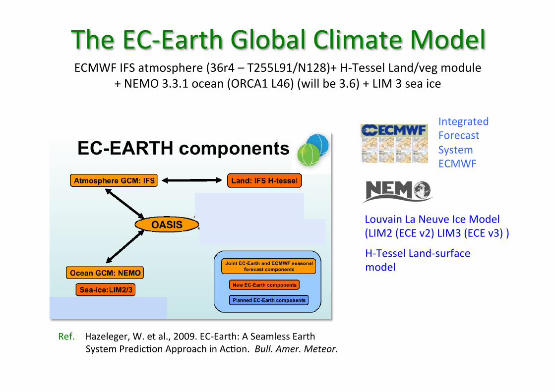
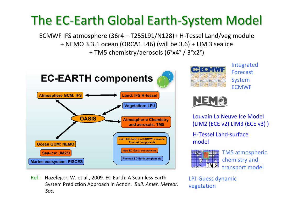
Observa(ons and modelling of precipita(on and the hydrological cycle: uncertain(es and downscaling Jost von Hardenberg Elisa Palazzi – Silvia Terzago ISACCNR, Torino with: L. Filippi, P. Davini, D. D’Onofrio (ISACCNR)
Transcript
Observa(ons and modelling of precipita(on and the hydrological cycle:
uncertain(es and downscaling
Jost von Hardenberg -‐ Elisa Palazzi – Silvia Terzago ISAC-‐CNR, Torino
with: L. Filippi, P. Davini, D. D’Onofrio (ISAC-‐CNR)
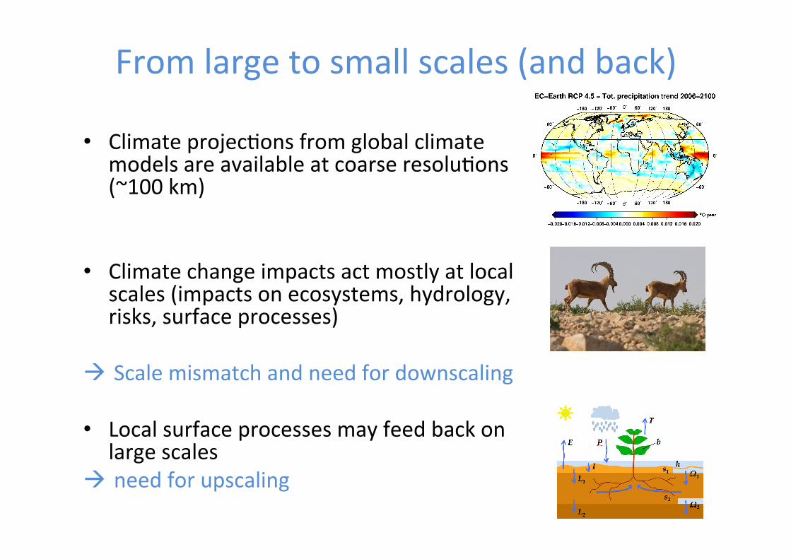
From large to small scales (and back)
• Climate projecOons from global climate models are available at coarse resoluOons (~100 km)
• Climate change impacts act mostly at local
scales (impacts on ecosystems, hydrology, risks, surface processes)
à Scale mismatch and need for downscaling
• Local surface processes may feed back on large scales
-‐ Examples of applicaOons to precipitaOon and snow
depth in the mountains (Karakoram-‐Himalaya and the Alps)
using the CMIP5 Global Climate Models and
the EC-‐Earth GCM
Winter Westerlies
Indian summer Monsoon
ITCZ (NH SUMMER)
L
L
HKK
Himalaya
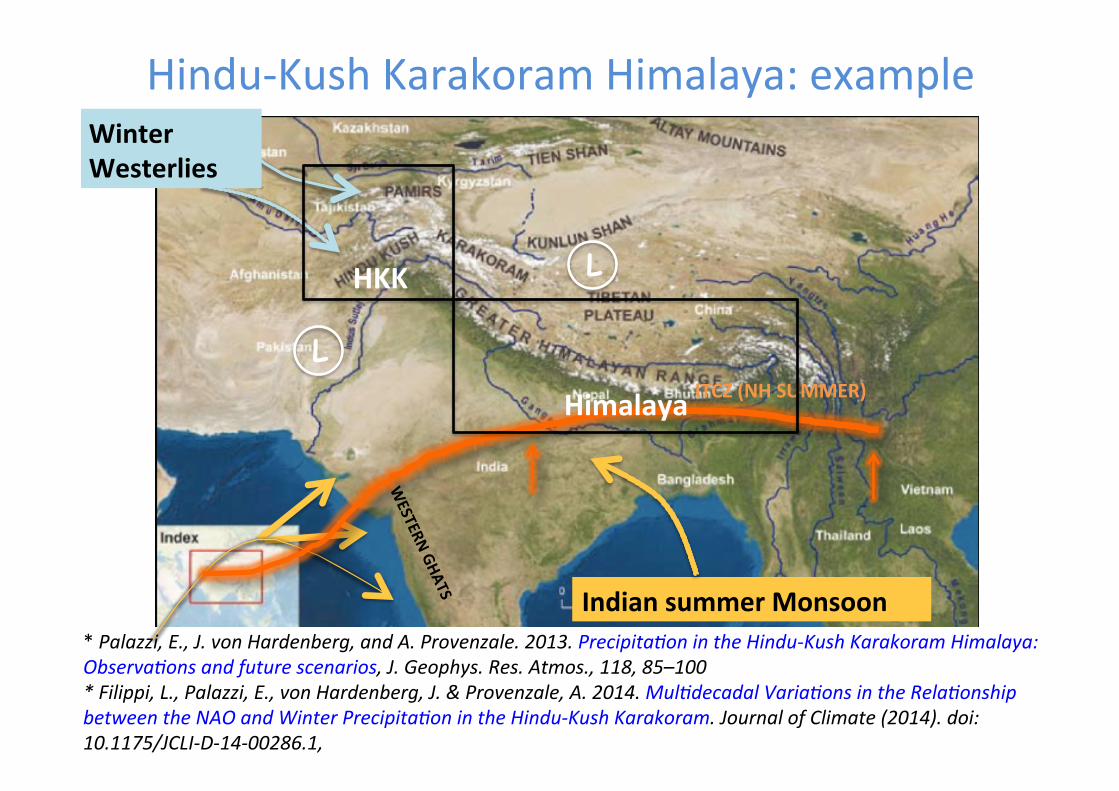
Hindu-‐Kush Karakoram Himalaya: example
* Palazzi, E., J. von Hardenberg, and A. Provenzale. 2013. Precipita<on in the Hindu-‐Kush Karakoram Himalaya: Observa<ons and future scenarios, J. Geophys. Res. Atmos., 118, 85–100 * Filippi, L., Palazzi, E., von Hardenberg, J. & Provenzale, A. 2014. Mul<decadal Varia<ons in the Rela<onship between the NAO and Winter Precipita<on in the Hindu-‐Kush Karakoram. Journal of Climate (2014). doi:10.1175/JCLI-‐D-‐14-‐00286.1,
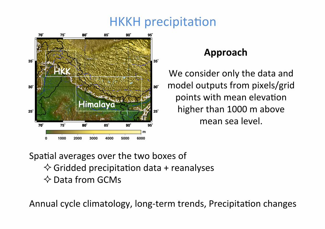
SpaOal averages over the two boxes of ² Gridded precipitaOon data + reanalyses ² Data from GCMs
We consider only the data and model outputs from pixels/grid points with mean elevaOon higher than 1000 m above
mean sea level.
HKK
Himalaya
Approach
HKKH precipitaOon
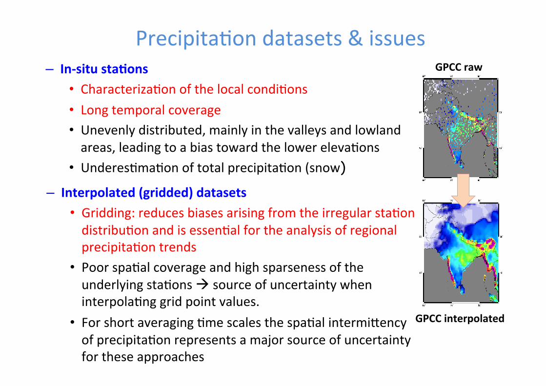
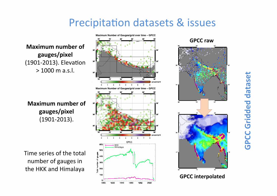
– In-‐situ sta(ons • CharacterizaOon of the local condiOons • Long temporal coverage • Unevenly distributed, mainly in the valleys and lowland areas, leading to a bias toward the lower elevaOons
• UnderesOmaOon of total precipitaOon (snow) – Interpolated (gridded) datasets
• Gridding: reduces biases arising from the irregular staOon distribuOon and is essenOal for the analysis of regional precipitaOon trends
• Poor spaOal coverage and high sparseness of the underlying staOons à source of uncertainty when interpolaOng grid point values.
• For short averaging Ome scales the spaOal intermi^ency of precipitaOon represents a major source of uncertainty for these approaches
PrecipitaOon datasets & issues GPCC raw
GPCC interpolated
Maximum Number of Gauges/grid over time − CRU
70˚
70˚
75˚
75˚
80˚
80˚
85˚
85˚
90˚
90˚
95˚
95˚
25˚ 25˚
30˚ 30˚
35˚ 35˚
0 1 2 3 4 5 6 7 8
gauges/grid70˚
70˚
75˚
75˚
80˚
80˚
85˚
85˚
90˚
90˚
95˚
95˚
25˚ 25˚
30˚ 30˚
35˚ 35˚
Maximum Number of Gauges/grid over time − GPCC
70˚
70˚
75˚
75˚
80˚
80˚
85˚
85˚
90˚
90˚
95˚
95˚
25˚ 25˚
30˚ 30˚
35˚ 35˚
0 1 2 3 4 5 6 7 8
gauges/grid70˚
70˚
75˚
75˚
80˚
80˚
85˚
85˚
90˚
90˚
95˚
95˚
25˚ 25˚
30˚ 30˚
35˚ 35˚
Maximum number of gauges/pixel
(1901-‐2013). ElevaOon > 1000 m a.s.l.
Maximum number of gauges/pixel (1901-‐2013).
Time series of the total number of gauges in the HKK and Himalaya
GPCC raw
GPCC interpolated
GPC
C Grid
ded da
taset
PrecipitaOon datasets & issues
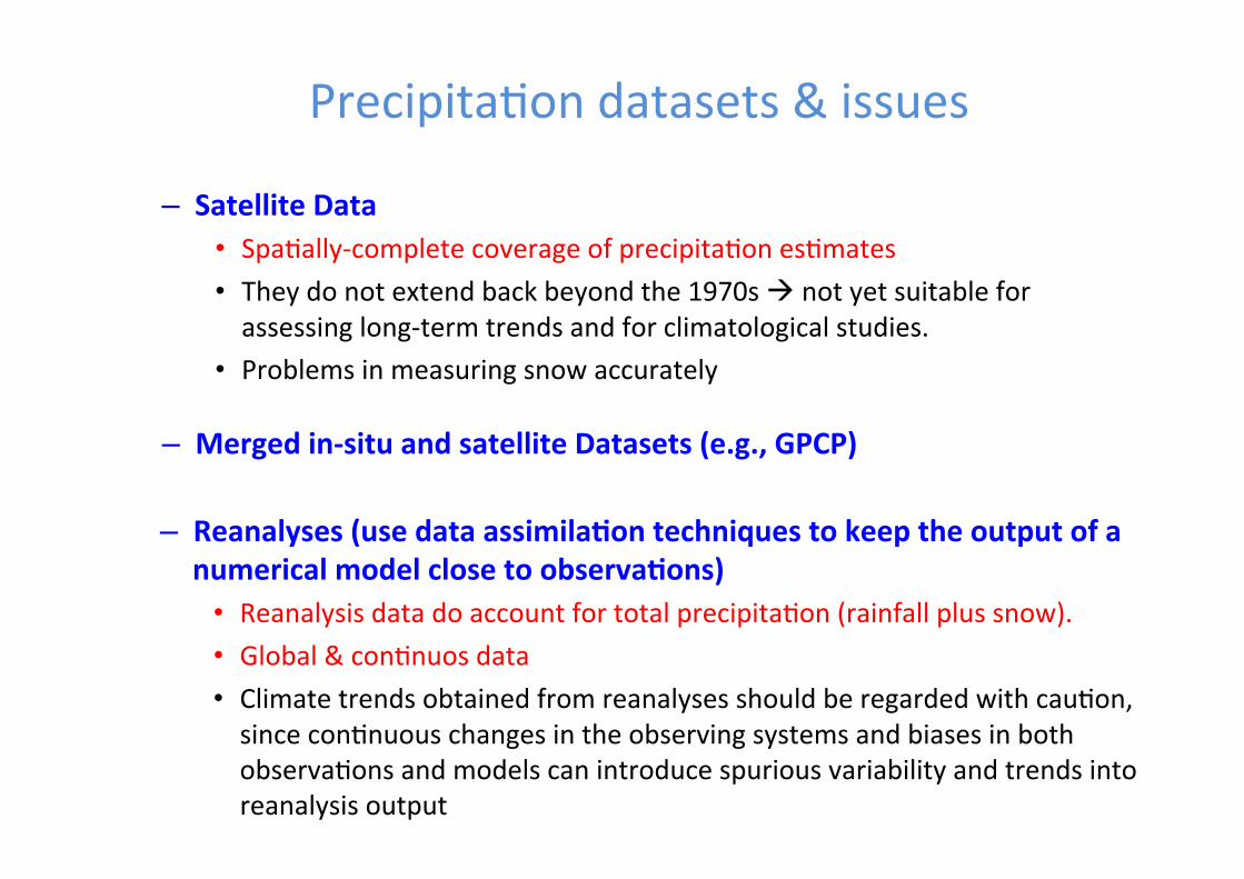
– Satellite Data • SpaOally-‐complete coverage of precipitaOon esOmates • They do not extend back beyond the 1970s à not yet suitable for assessing long-‐term trends and for climatological studies.
• Problems in measuring snow accurately
PrecipitaOon datasets & issues
– Merged in-‐situ and satellite Datasets (e.g., GPCP)
– Reanalyses (use data assimila(on techniques to keep the output of a numerical model close to observa(ons)
• Reanalysis data do account for total precipitaOon (rainfall plus snow). • Global & conOnuos data • Climate trends obtained from reanalyses should be regarded with cauOon, since conOnuous changes in the observing systems and biases in both observaOons and models can introduce spurious variability and trends into reanalysis output
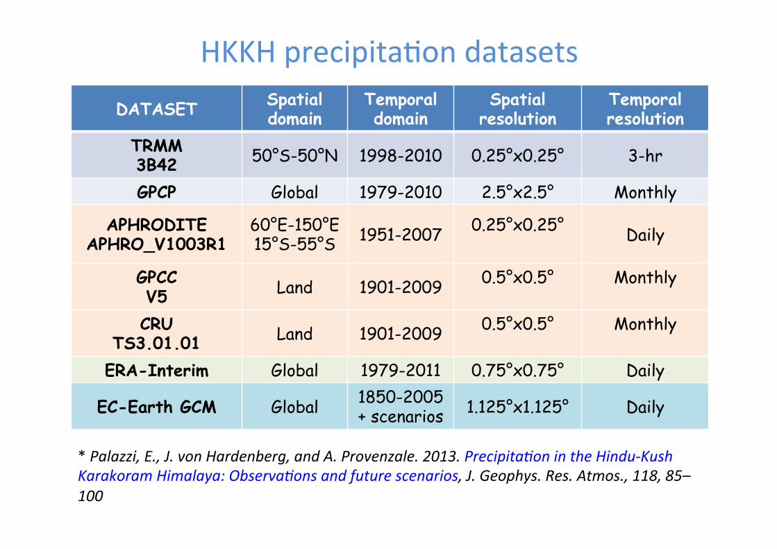
DATASET Spatial domain
Temporal domain
Spatial resolution
Temporal resolution
TRMM 3B42 50°S-50°N 1998-2010 0.25°x0.25° 3-hr
GPCP Global 1979-2010 2.5°x2.5° Monthly
APHRODITE APHRO_V1003R1
60°E-150°E 15°S-55°S 1951-2007 0.25°x0.25°
Daily
GPCC V5 Land 1901-2009 0.5°x0.5°
Monthly
CRU
TS3.01.01 Land 1901-2009 0.5°x0.5°
Monthly
ERA-Interim Global 1979-2011 0.75°x0.75° Daily
EC-Earth GCM Global 1850-2005 + scenarios 1.125°x1.125° Daily
HKKH precipitaOon datasets
* Palazzi, E., J. von Hardenberg, and A. Provenzale. 2013. Precipita<on in the Hindu-‐Kush Karakoram Himalaya: Observa<ons and future scenarios, J. Geophys. Res. Atmos., 118, 85–100
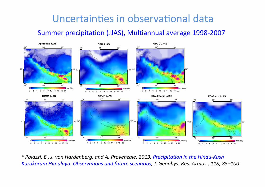
Summer precipitaOon (JJAS), MulOannual average 1998-‐2007 Aphrodite JJAS
70˚
70˚
80˚
80˚
90˚
90˚
30˚ 30˚
0 2 4 6 8 10 12 14 16 18 20mm/day
CRU JJAS
70˚
70˚
80˚
80˚
90˚
90˚
30˚ 30˚
0 2 4 6 8 10 12 14 16 18 20mm/day
GPCC JJAS
70˚
70˚
80˚
80˚
90˚
90˚
30˚ 30˚
0 2 4 6 8 10 12 14 16 18 20mm/day
TRMM JJAS
70˚
70˚
80˚
80˚
90˚
90˚
30˚ 30˚
0 2 4 6 8 10 12 14 16 18 20mm/day
GPCP JJAS
70˚
70˚
80˚
80˚
90˚
90˚
30˚ 30˚
0 2 4 6 8 10 12 14 16 18 20mm/day
ERA−Interim JJAS
70˚
70˚
80˚
80˚
90˚
90˚
30˚ 30˚
0 2 4 6 8 10 12 14 16 18 20mm/day
EC−Earth JJAS
70˚
70˚
80˚
80˚
90˚
90˚
30˚ 30˚
0 2 4 6 8 10 12 14 16 18 20mm/day
UncertainOes in observaOonal data
* Palazzi, E., J. von Hardenberg, and A. Provenzale. 2013. Precipita<on in the Hindu-‐Kush Karakoram Himalaya: Observa<ons and future scenarios, J. Geophys. Res. Atmos., 118, 85–100
Aphrodite DJFMA
70˚
70˚
80˚
80˚
90˚
90˚
30˚ 30˚
0 1 2 3 4 5mm/day
CRU DJFMA
70˚
70˚
80˚
80˚
90˚
90˚
30˚ 30˚
0 1 2 3 4 5mm/day
GPCC DJFMA
70˚
70˚
80˚
80˚
90˚
90˚
30˚ 30˚
0 1 2 3 4 5mm/day
TRMM DJFMA
70˚
70˚
80˚
80˚
90˚
90˚
30˚ 30˚
0 1 2 3 4 5mm/day
GPCP DJFMA
70˚
70˚
80˚
80˚
90˚
90˚
30˚ 30˚
0 1 2 3 4 5mm/day
ERA−Interim DJFMA
70˚
70˚
80˚
80˚
90˚
90˚
30˚ 30˚
0 1 2 3 4 5mm/day
EC−Earth DJFMA
70˚
70˚
80˚
80˚
90˚
90˚
30˚ 30˚
0 1 2 3 4 5mm/day
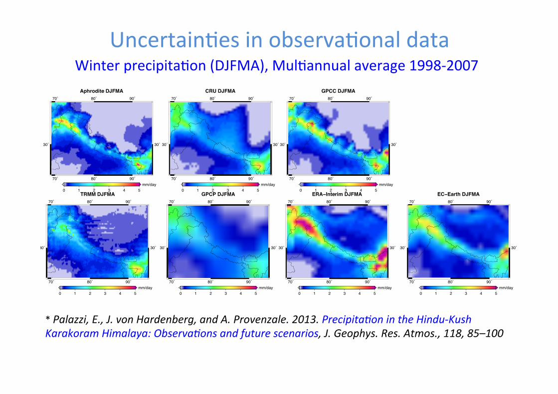
Winter precipitaOon (DJFMA), MulOannual average 1998-‐2007
* Palazzi, E., J. von Hardenberg, and A. Provenzale. 2013. Precipita<on in the Hindu-‐Kush Karakoram Himalaya: Observa<ons and future scenarios, J. Geophys. Res. Atmos., 118, 85–100
UncertainOes in observaOonal data
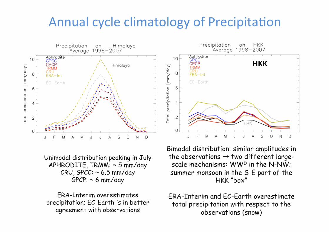
Bimodal distribution: similar amplitudes in the observations → two different large-scale mechanisms: WWP in the N-NW; summer monsoon in the S-E part of the
HKK “box”
ERA-Interim and EC-Earth overestimate total precipitation with respect to the
observations (snow)
Unimodal distribution peaking in July APHRODITE, TRMM: ~ 5 mm/day
CRU, GPCC: ~ 6.5 mm/day GPCP: ~ 6 mm/day
ERA-Interim overestimates
precipitation; EC-Earth is in better agreement with observations
HKK Himalaya
Annual cycle climatology of PrecipitaOon
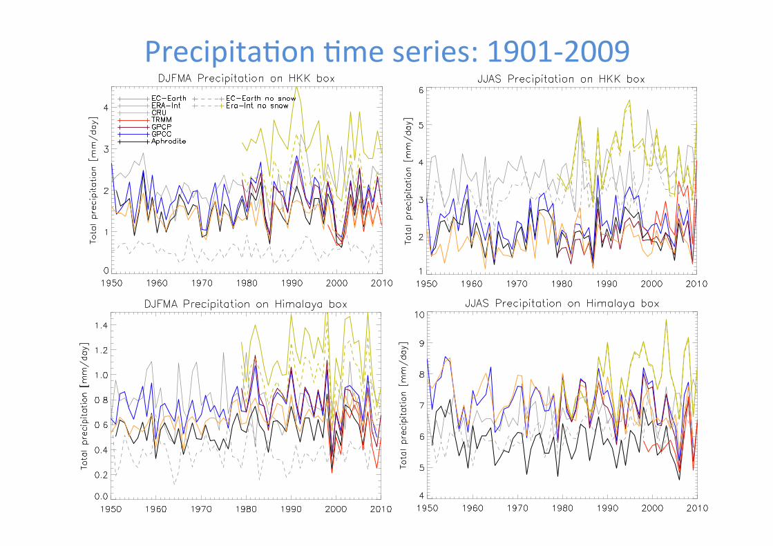
PrecipitaOon Ome series: 1901-‐2009
http
://c
mip-p
cmdi
.llnl.go
v/cm
ip5/
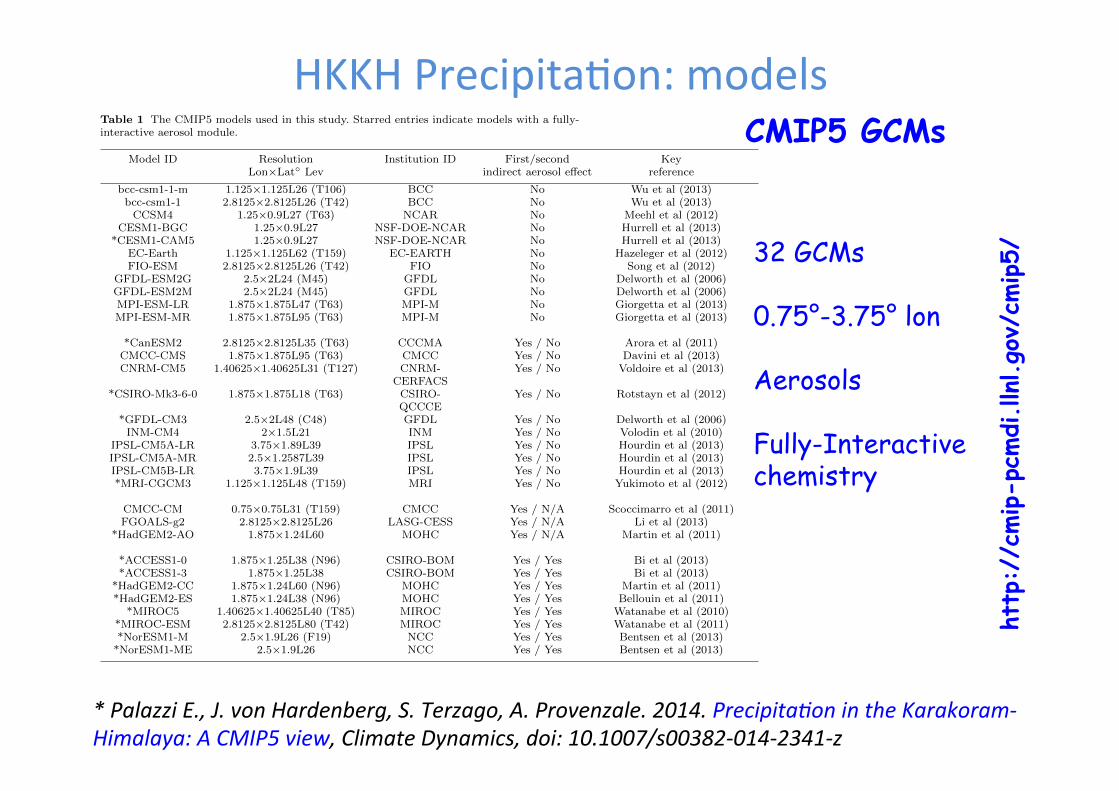
CMIP5 GCMs Precipitation in the Karakoram-Himalaya: A CMIP5 view 35
Table 1 The CMIP5 models used in this study. Starred entries indicate models with a fully-interactive aerosol module.
Model ID Resolution Institution ID First/second KeyLon⇥Lat� Lev indirect aerosol e↵ect reference
bcc-csm1-1-m 1.125⇥1.125L26 (T106) BCC No Wu et al (2013)bcc-csm1-1 2.8125⇥2.8125L26 (T42) BCC No Wu et al (2013)CCSM4 1.25⇥0.9L27 (T63) NCAR No Meehl et al (2012)
CESM1-BGC 1.25⇥0.9L27 NSF-DOE-NCAR No Hurrell et al (2013)*CESM1-CAM5 1.25⇥0.9L27 NSF-DOE-NCAR No Hurrell et al (2013)
EC-Earth 1.125⇥1.125L62 (T159) EC-EARTH No Hazeleger et al (2012)FIO-ESM 2.8125⇥2.8125L26 (T42) FIO No Song et al (2012)
GFDL-ESM2G 2.5⇥2L24 (M45) GFDL No Delworth et al (2006)GFDL-ESM2M 2.5⇥2L24 (M45) GFDL No Delworth et al (2006)MPI-ESM-LR 1.875⇥1.875L47 (T63) MPI-M No Giorgetta et al (2013)MPI-ESM-MR 1.875⇥1.875L95 (T63) MPI-M No Giorgetta et al (2013)
*CanESM2 2.8125⇥2.8125L35 (T63) CCCMA Yes / No Arora et al (2011)CMCC-CMS 1.875⇥1.875L95 (T63) CMCC Yes / No Davini et al (2013)CNRM-CM5 1.40625⇥1.40625L31 (T127) CNRM- Yes / No Voldoire et al (2013)
CERFACS*CSIRO-Mk3-6-0 1.875⇥1.875L18 (T63) CSIRO- Yes / No Rotstayn et al (2012)
QCCCE*GFDL-CM3 2.5⇥2L48 (C48) GFDL Yes / No Delworth et al (2006)INM-CM4 2⇥1.5L21 INM Yes / No Volodin et al (2010)
IPSL-CM5A-LR 3.75⇥1.89L39 IPSL Yes / No Hourdin et al (2013)IPSL-CM5A-MR 2.5⇥1.2587L39 IPSL Yes / No Hourdin et al (2013)IPSL-CM5B-LR 3.75⇥1.9L39 IPSL Yes / No Hourdin et al (2013)*MRI-CGCM3 1.125⇥1.125L48 (T159) MRI Yes / No Yukimoto et al (2012)
CMCC-CM 0.75⇥0.75L31 (T159) CMCC Yes / N/A Scoccimarro et al (2011)FGOALS-g2 2.8125⇥2.8125L26 LASG-CESS Yes / N/A Li et al (2013)
*HadGEM2-AO 1.875⇥1.24L60 MOHC Yes / N/A Martin et al (2011)
*ACCESS1-0 1.875⇥1.25L38 (N96) CSIRO-BOM Yes / Yes Bi et al (2013)*ACCESS1-3 1.875⇥1.25L38 CSIRO-BOM Yes / Yes Bi et al (2013)
*HadGEM2-CC 1.875⇥1.24L60 (N96) MOHC Yes / Yes Martin et al (2011)*HadGEM2-ES 1.875⇥1.24L38 (N96) MOHC Yes / Yes Bellouin et al (2011)
*MIROC5 1.40625⇥1.40625L40 (T85) MIROC Yes / Yes Watanabe et al (2010)*MIROC-ESM 2.8125⇥2.8125L80 (T42) MIROC Yes / Yes Watanabe et al (2011)*NorESM1-M 2.5⇥1.9L26 (F19) NCC Yes / Yes Bentsen et al (2013)*NorESM1-ME 2.5⇥1.9L26 NCC Yes / Yes Bentsen et al (2013)
* Palazzi E., J. von Hardenberg, S. Terzago, A. Provenzale. 2014. Precipita<on in the Karakoram-‐Himalaya: A CMIP5 view, Climate Dynamics, doi: 10.1007/s00382-‐014-‐2341-‐z
CMCC−CM JJAS
70˚
70˚
80˚
80˚
90˚
90˚
30˚ 30˚
0 2 4 6 8 10 12 14 16 18 20
mm/day70˚
70˚
80˚
80˚
90˚
90˚
30˚ 30˚
CESM1−CAM5 JJAS
70˚
70˚
80˚
80˚
90˚
90˚
30˚ 30˚
0 2 4 6 8 10 12 14 16 18 20
mm/day70˚
70˚
80˚
80˚
90˚
90˚
30˚ 30˚
MIROC5 JJAS
70˚
70˚
80˚
80˚
90˚
90˚
30˚ 30˚
0 2 4 6 8 10 12 14 16 18 20
mm/day70˚
70˚
80˚
80˚
90˚
90˚
30˚ 30˚
HadGEM2−ES JJAS
70˚
70˚
80˚
80˚
90˚
90˚
30˚ 30˚
0 2 4 6 8 10 12 14 16 18 20
mm/day70˚
70˚
80˚
80˚
90˚
90˚
30˚ 30˚
inmcm4 JJAS
70˚
70˚
80˚
80˚
90˚
90˚
30˚ 30˚
0 2 4 6 8 10 12 14 16 18 20
mm/day70˚
70˚
80˚
80˚
90˚
90˚
30˚ 30˚
NorESM1−ME JJAS
70˚
70˚
80˚
80˚
90˚
90˚
30˚ 30˚
0 2 4 6 8 10 12 14 16 18 20
mm/day70˚
70˚
80˚
80˚
90˚
90˚
30˚ 30˚
FGOALS−g2 JJAS
70˚
70˚
80˚
80˚
90˚
90˚
30˚ 30˚
0 2 4 6 8 10 12 14 16 18 20
mm/day70˚
70˚
80˚
80˚
90˚
90˚
30˚ 30˚
IPSL−CM5A−LR JJAS
70˚
70˚
80˚
80˚
90˚
90˚
30˚ 30˚
0 2 4 6 8 10 12 14 16 18 20
mm/day70˚
70˚
80˚
80˚
90˚
90˚
30˚ 30˚
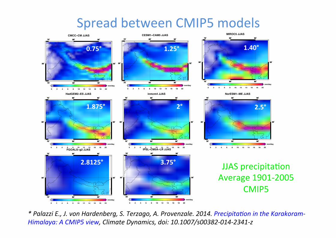
0.75° 1.25° 1.40°
1.875° 2° 2.5°
2.8125° 3.75°
Spread between CMIP5 models
JJAS precipitaOon Average 1901-‐2005
CMIP5
* Palazzi E., J. von Hardenberg, S. Terzago, A. Provenzale. 2014. Precipita<on in the Karakoram-‐Himalaya: A CMIP5 view, Climate Dynamics, doi: 10.1007/s00382-‐014-‐2341-‐z
CMCC−CM DJFMA
70˚
70˚
80˚
80˚
90˚
90˚
30˚ 30˚
0 1 2 3 4 5 6 7 8
mm/day70˚
70˚
80˚
80˚
90˚
90˚
30˚ 30˚
CESM1−CAM5 DJFMA
70˚
70˚
80˚
80˚
90˚
90˚
30˚ 30˚
0 1 2 3 4 5 6 7 8
mm/day70˚
70˚
80˚
80˚
90˚
90˚
30˚ 30˚
MIROC5 DJFMA
70˚
70˚
80˚
80˚
90˚
90˚
30˚ 30˚
0 1 2 3 4 5 6 7 8
mm/day70˚
70˚
80˚
80˚
90˚
90˚
30˚ 30˚
HadGEM2−ES DJFMA
70˚
70˚
80˚
80˚
90˚
90˚
30˚ 30˚
0 1 2 3 4 5 6 7 8
mm/day70˚
70˚
80˚
80˚
90˚
90˚
30˚ 30˚
inmcm4 DJFMA
70˚
70˚
80˚
80˚
90˚
90˚
30˚ 30˚
0 1 2 3 4 5 6 7 8
mm/day70˚
70˚
80˚
80˚
90˚
90˚
30˚ 30˚
NorESM1−ME DJFMA
70˚
70˚
80˚
80˚
90˚
90˚
30˚ 30˚
0 1 2 3 4 5 6 7 8
mm/day70˚
70˚
80˚
80˚
90˚
90˚
30˚ 30˚
FGOALS−g2 DJFMA
70˚
70˚
80˚
80˚
90˚
90˚
30˚ 30˚
0 1 2 3 4 5 6 7 8
mm/day70˚
70˚
80˚
80˚
90˚
90˚
30˚ 30˚
IPSL−CM5A−LR DJFMA
70˚
70˚
80˚
80˚
90˚
90˚
30˚ 30˚
0 1 2 3 4 5 6 7 8
mm/day70˚
70˚
80˚
80˚
90˚
90˚
30˚ 30˚
0.75° 1.25° 1.40°
1.875° 2° 2.5°
2.8125° 3.75° DJFMA precipitaOon Average 1901-‐2005
CMIP5
Spread between CMIP5 models
* Palazzi E., J. von Hardenberg, S. Terzago, A. Provenzale. 2014. Precipita<on in the Karakoram-‐Himalaya: A CMIP5 view, Climate Dynamics, doi: 10.1007/s00382-‐014-‐2341-‐z
36 Elisa Palazzi et al.
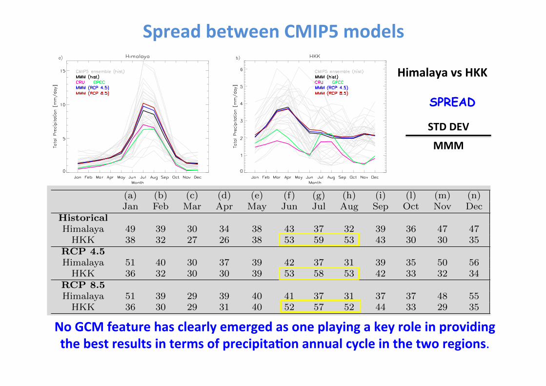
Table 2 Multi-annual mean monthly (Jan to Dec) and seasonal (DJFMA and JJAS) valuesof the coe�cient of variation (CV, the ratio of the multi-model standard deviation to themulti-model mean expressed as a percentage [%] of the multi-model mean) in the Himalayaand HKK sub-regions. The time averages are performed over the period 1901-2005 (historicalperiod) and over the years 2006-2100 for the future scenarios. Please note that the monthlyCV values are obtained from the multiannual mean of montly precipitation from each CMIP5model shown in Figs. 2a and 2b, while the DJFMA and JJAS CV values are obtained byaveraging in time the seasonal precipitation time series from each model shown in Fig. 3.
(a) (b) (c) (d) (e) (f) (g) (h) (i) (l) (m) (n) (o) (p)Jan Feb Mar Apr May Jun Jul Aug Sep Oct Nov Dec DJFMA JJAS
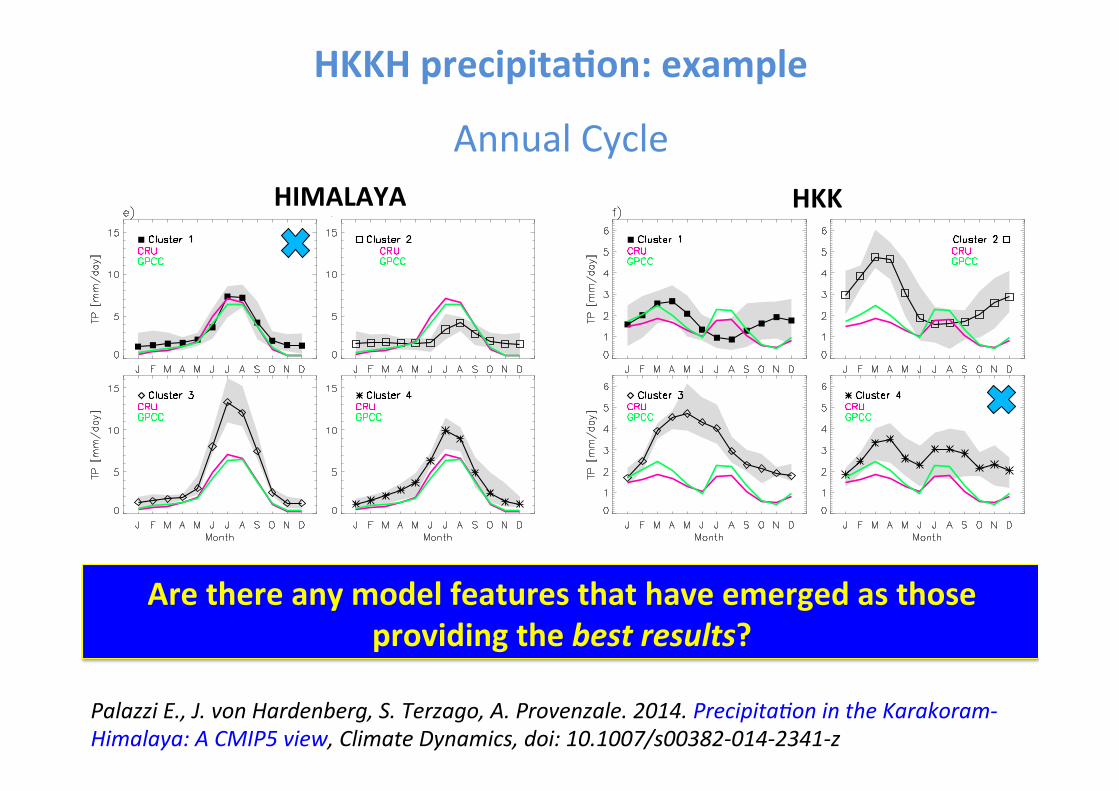
No GCM feature has clearly emerged as one playing a key role in providing the best results in terms of precipita(on annual cycle in the two regions.
Figure 4:
Spread between CMIP5 models
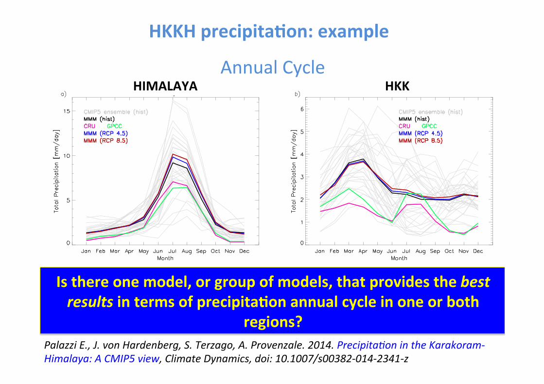
HKKH precipita(on: example
Figure 4:HIMALAYA HKK
Palazzi E., J. von Hardenberg, S. Terzago, A. Provenzale. 2014. Precipita<on in the Karakoram-‐Himalaya: A CMIP5 view, Climate Dynamics, doi: 10.1007/s00382-‐014-‐2341-‐z
Is there one model, or group of models, that provides the best results in terms of precipita(on annual cycle in one or both
regions?
Annual Cycle
HKKH precipita(on: example
Figure 4:
Palazzi E., J. von Hardenberg, S. Terzago, A. Provenzale. 2014. Precipita<on in the Karakoram-‐Himalaya: A CMIP5 view, Climate Dynamics, doi: 10.1007/s00382-‐014-‐2341-‐z
HIMALAYA HKK
Are there any model features that have emerged as those providing the best results?
Annual Cycle
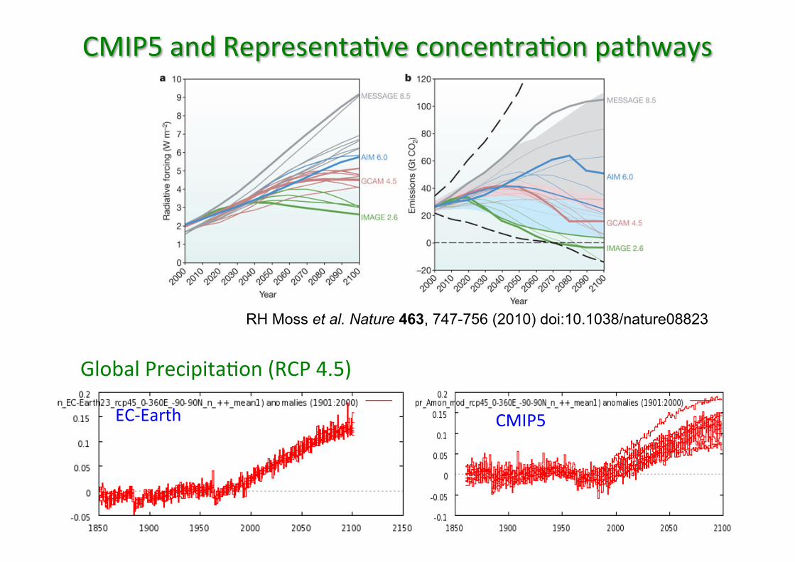
CMIP5 and RepresentaOve concentraOon pathways
EC-‐Earth CMIP5
Global PrecipitaOon (RCP 4.5)
RH Moss et al. Nature 463, 747-756 (2010) doi:10.1038/nature08823
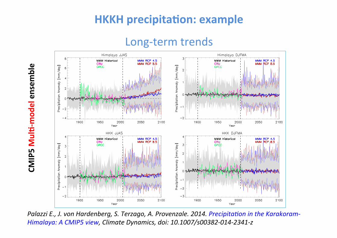
HKKH precipita(on: example
Palazzi E., J. von Hardenberg, S. Terzago, A. Provenzale. 2014. Precipita<on in the Karakoram-‐Himalaya: A CMIP5 view, Climate Dynamics, doi: 10.1007/s00382-‐014-‐2341-‐z
CMIP5 Mul(-‐mod
el ensem
ble
Long-‐term trends
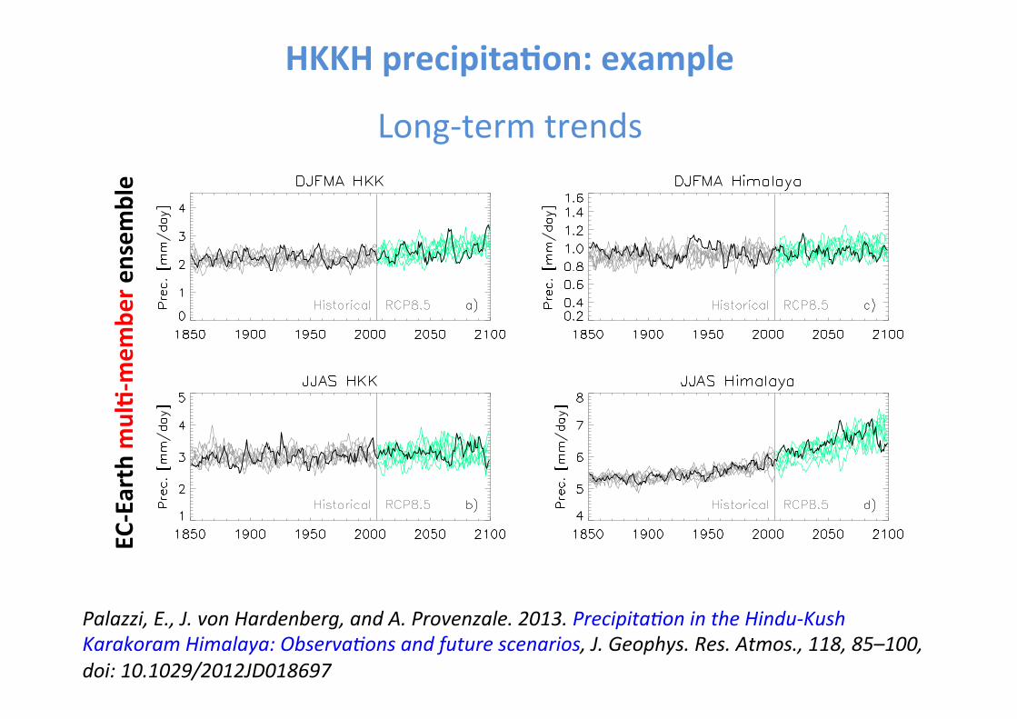
HKKH precipita(on: example
Palazzi, E., J. von Hardenberg, and A. Provenzale. 2013. Precipita<on in the Hindu-‐Kush Karakoram Himalaya: Observa<ons and future scenarios, J. Geophys. Res. Atmos., 118, 85–100, doi: 10.1029/2012JD018697
EC-‐Earth m
ul(-‐mem
ber e
nsem
ble
Long-‐term trends
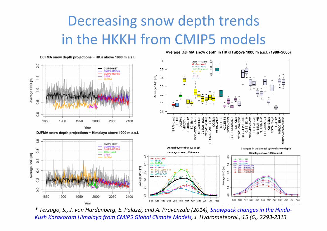
Decreasing snow depth trends in the HKKH from CMIP5 models
* Terzago, S., J. von Hardenberg, E. Palazzi, and A. Provenzale (2014), Snowpack changes in the Hindu-‐Kush Karakoram Himalaya from CMIP5 Global Climate Models, J. Hydrometeorol., 15 (6), 2293-‐2313
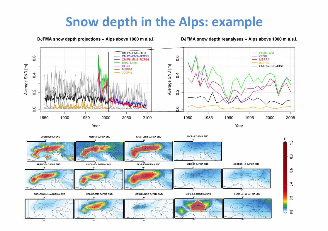
Snow depth in the Alps: example DJFMA snow depth projections � Alps above 1000 m a.s.l.
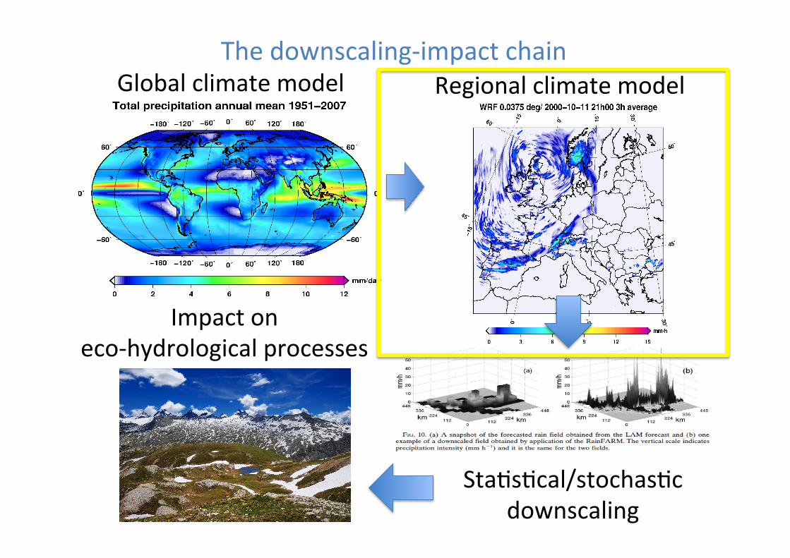
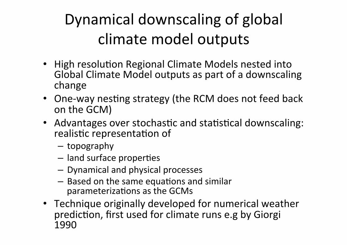
Dynamical downscaling of global climate model outputs
• High resoluOon Regional Climate Models nested into Global Climate Model outputs as part of a downscaling change
• One-‐way nesOng strategy (the RCM does not feed back on the GCM)
• Advantages over stochasOc and staOsOcal downscaling: realisOc representaOon of – topography – land surface properOes – Dynamical and physical processes – Based on the same equaOons and similar parameterizaOons as the GCMs
• Technique originally developed for numerical weather predicOon, first used for climate runs e.g by Giorgi 1990
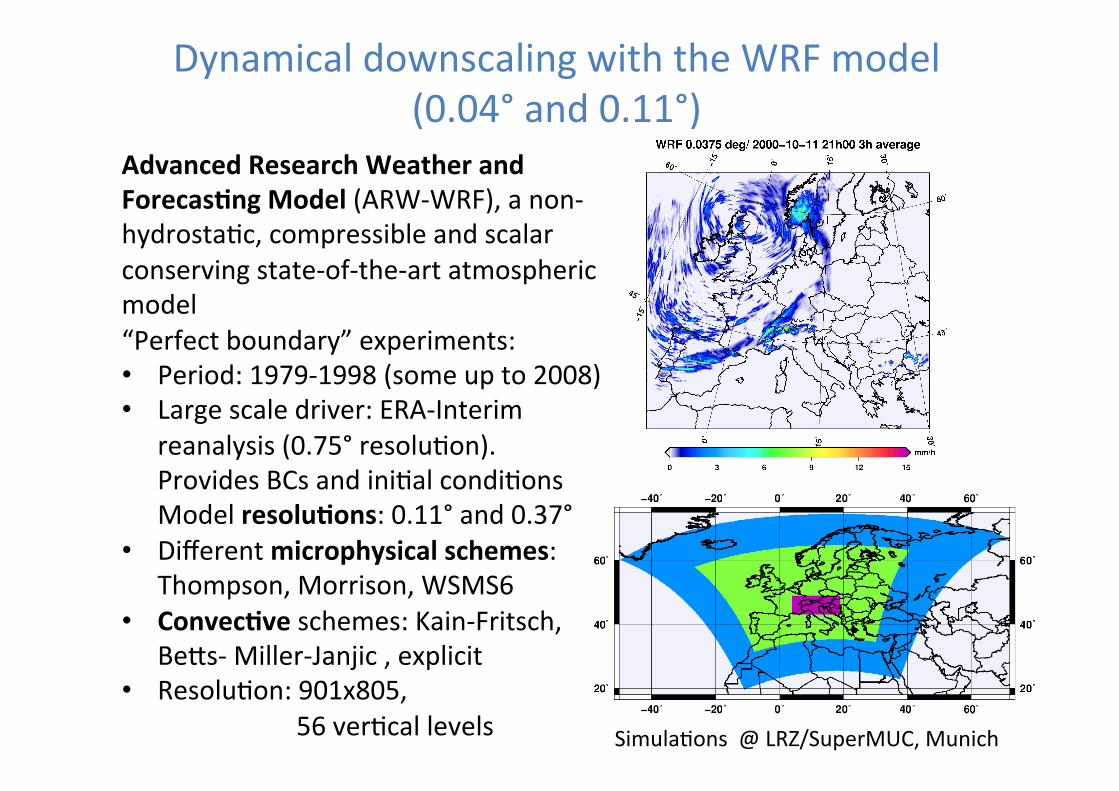
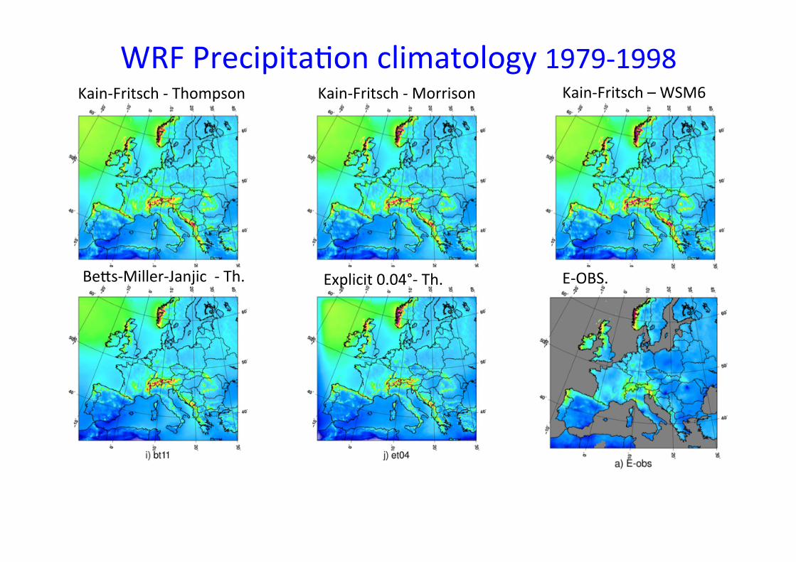
Dynamical downscaling with the WRF model (0.04° and 0.11°)
Advanced Research Weather and Forecas(ng Model (ARW-‐WRF), a non-‐hydrostaOc, compressible and scalar conserving state-‐of-‐the-‐art atmospheric model “Perfect boundary” experiments: • Period: 1979-‐1998 (some up to 2008) • Large scale driver: ERA-‐Interim
reanalysis (0.75° resoluOon). Provides BCs and iniOal condiOons Model resolu(ons: 0.11° and 0.37°
• Different microphysical schemes: Thompson, Morrison, WSMS6
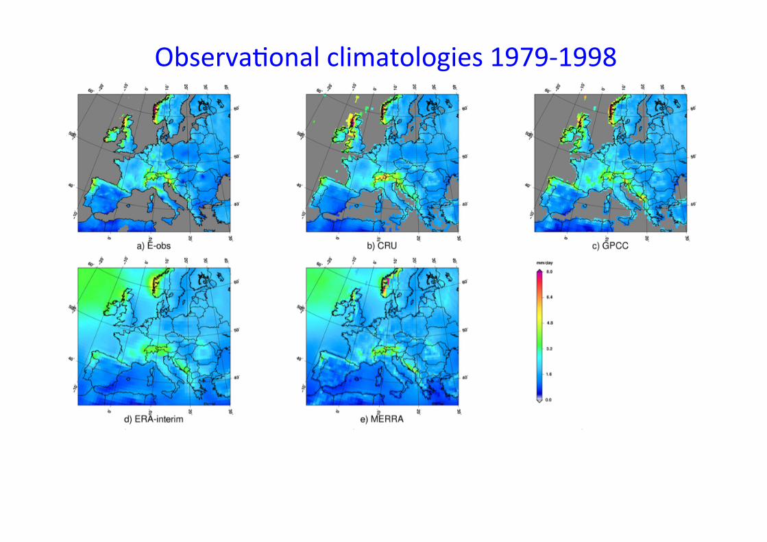
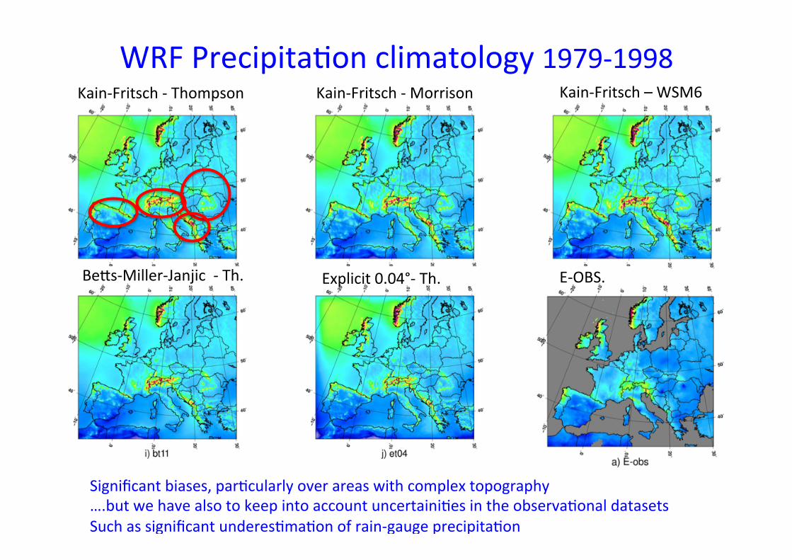
Significant biases, parOcularly over areas with complex topography ….but we have also to keep into account uncertainiOes in the observaOonal datasets Such as significant underesOmaOon of rain-‐gauge precipitaOon
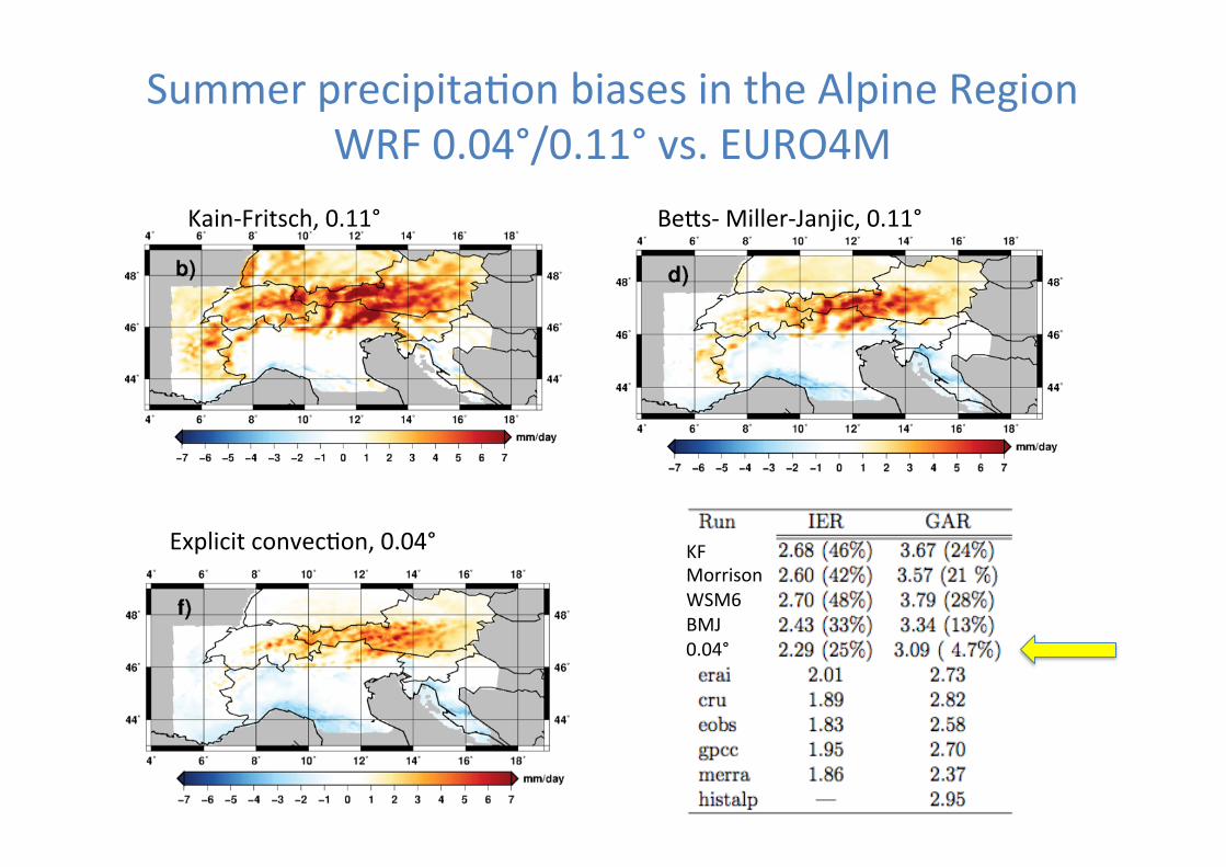
Summer precipitaOon biases in the Alpine Region WRF 0.04°/0.11° vs. EURO4M
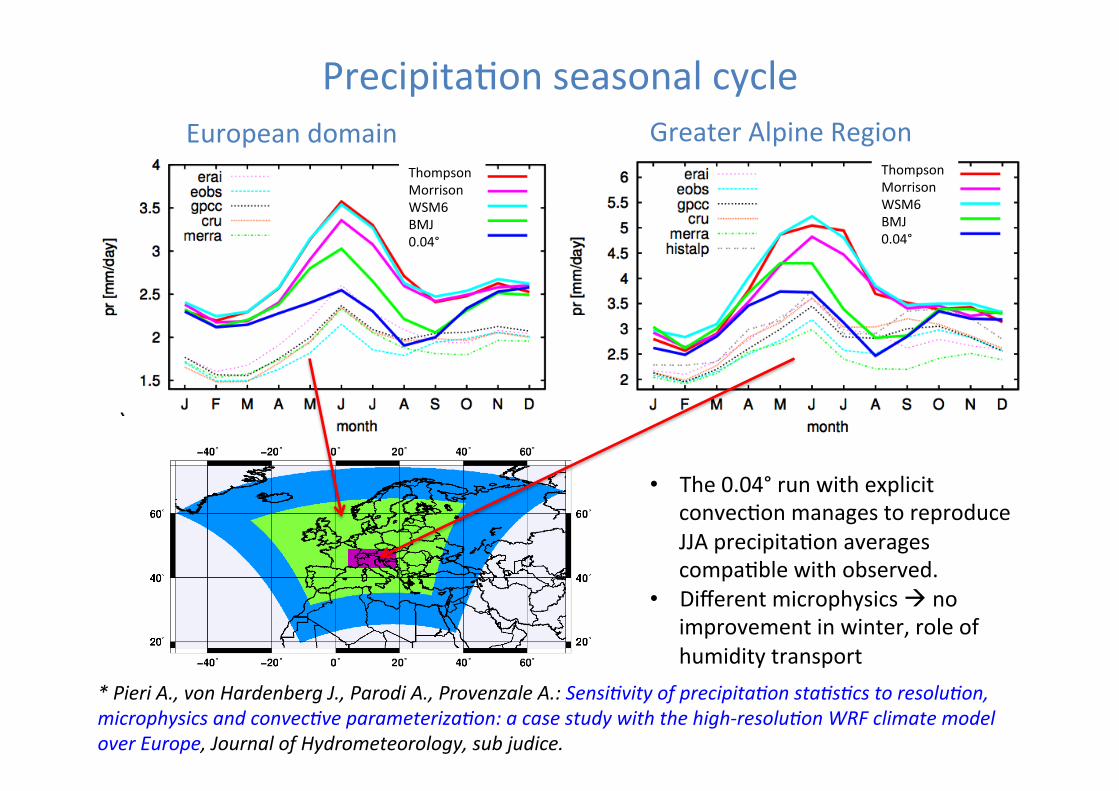
PrecipitaOon seasonal cycle European domain Greater Alpine Region
Thompson Morrison WSM6 BMJ 0.04°
Thompson Morrison WSM6 BMJ 0.04°
• The 0.04° run with explicit convecOon manages to reproduce JJA precipitaOon averages compaOble with observed.
• Different microphysics à no improvement in winter, role of humidity transport
* Pieri A., von Hardenberg J., Parodi A., Provenzale A.: Sensi<vity of precipita<on sta<s<cs to resolu<on, microphysics and convec<ve parameteriza<on: a case study with the high-‐resolu<on WRF climate model over Europe, Journal of Hydrometeorology, sub judice.
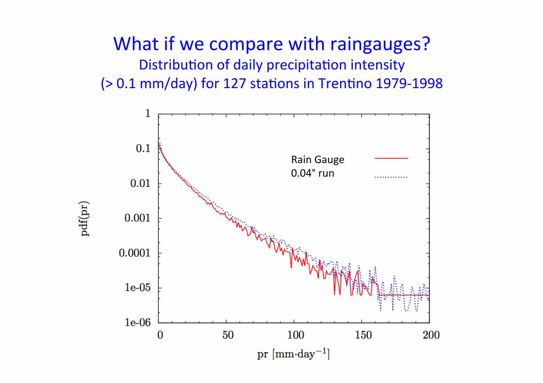
What if we compare with raingauges? DistribuOon of daily precipitaOon intensity
(> 0.1 mm/day) for 127 staOons in TrenOno 1979-‐1998
Rain Gauge 0.04° run
+%#$,%)-%.',/&)'#0&%) 1&2.#3,%)-%.',/&)'#0&%)
*/,454-,%65/#-7,54-)0#835-,%.32)
)
9':,-/)#3))&-#;7<0"#%#2.-,%):"#-&55&5)
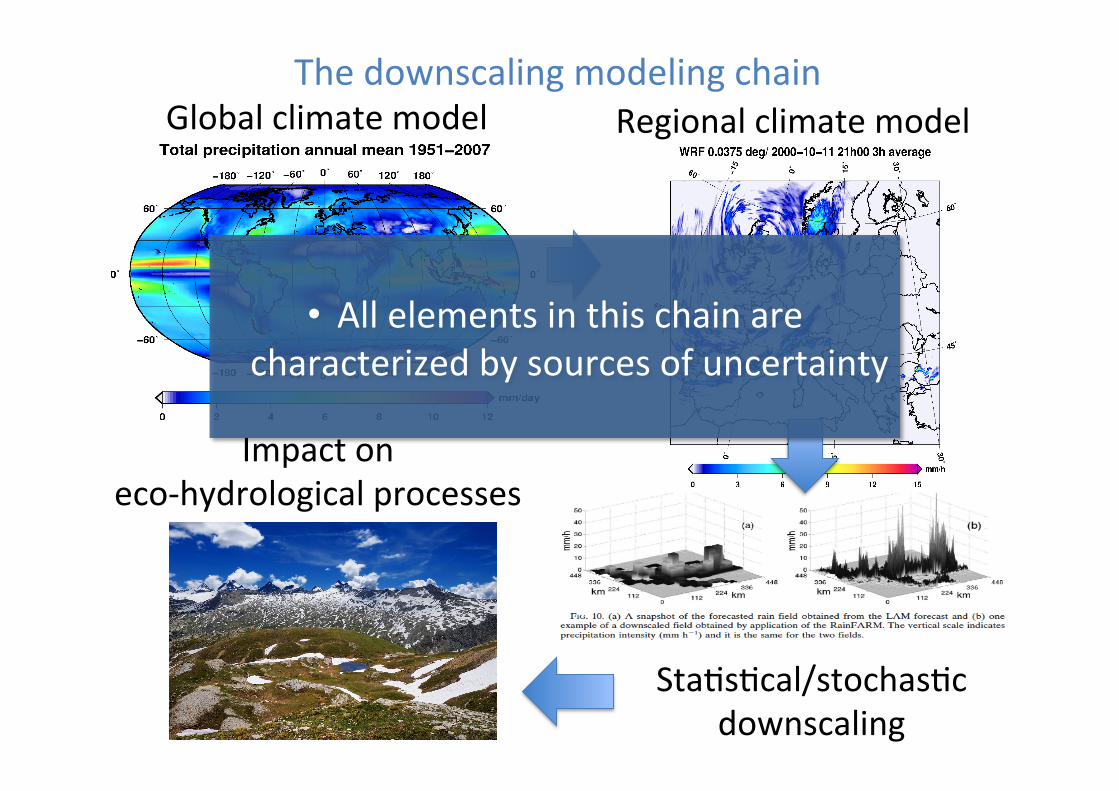
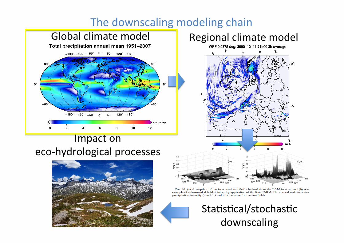
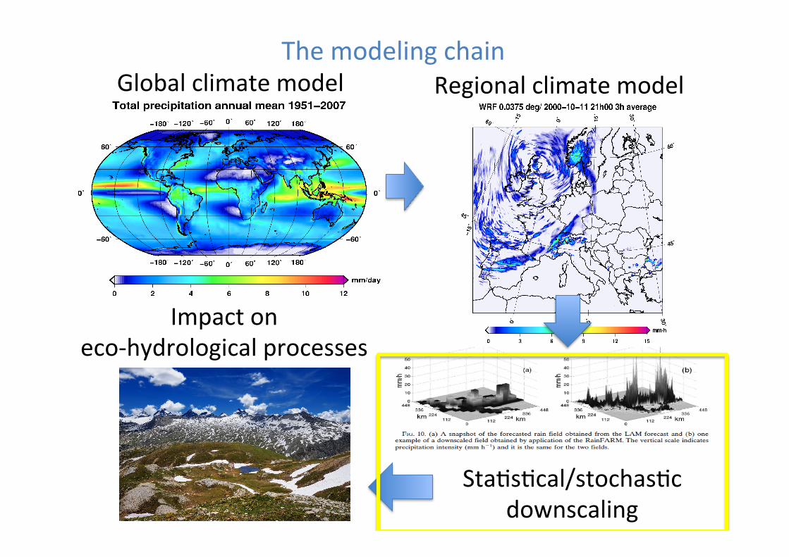
A:/!<#$%&'()*%+L*9.('1!':(*%!The modeling chain
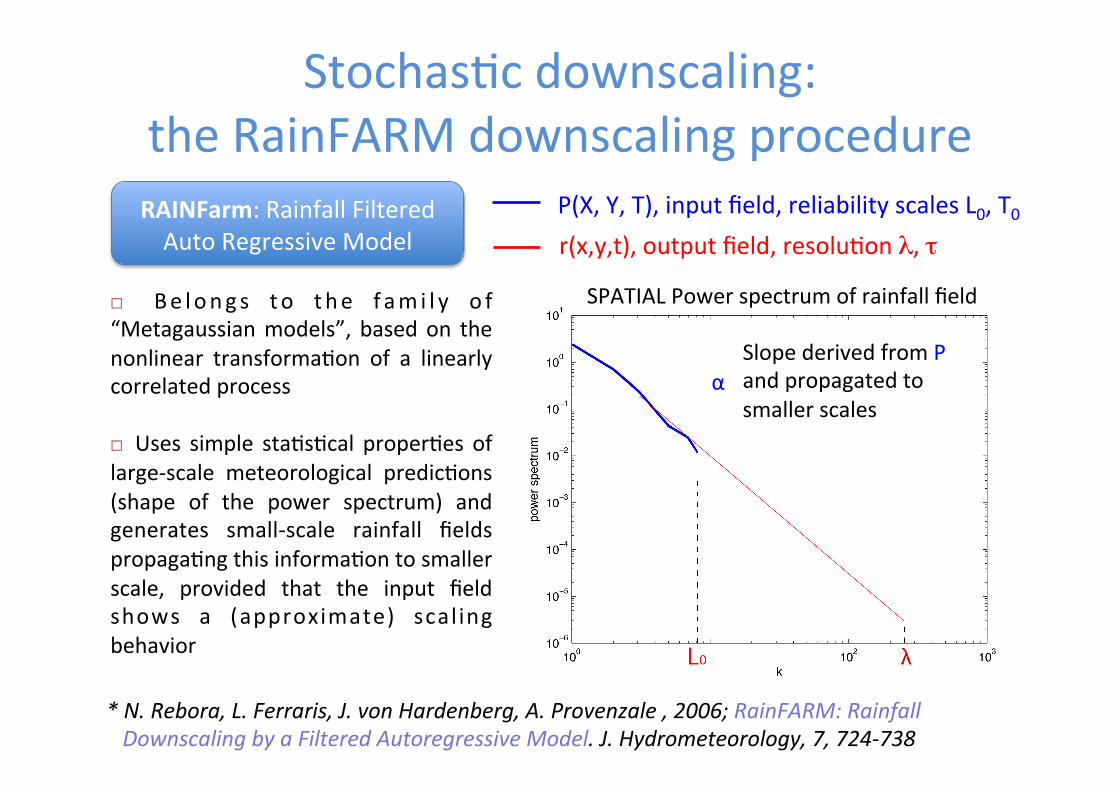
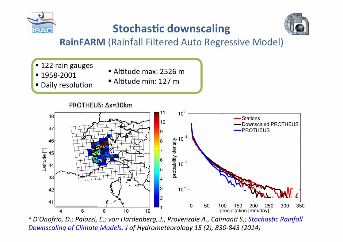
StochasOc downscaling: the RainFARM downscaling procedure
α Slope derived from P and propagated to smaller scales
¨ Be l ong s t o t he f am i l y o f “Metagaussian models”, based on the nonlinear transformaOon of a linearly correlated process
¨ Uses simple staOsOcal properOes of large-‐scale meteorological predicOons (shape of the power spectrum) and generates small-‐scale rainfall fields propagaOng this informaOon to smaller scale, provided that the input field shows a (approximate) scal ing behavior
* N. Rebora, L. Ferraris, J. von Hardenberg, A. Provenzale , 2006; RainFARM: Rainfall Downscaling by a Filtered Autoregressive Model. J. Hydrometeorology, 7, 724-‐738
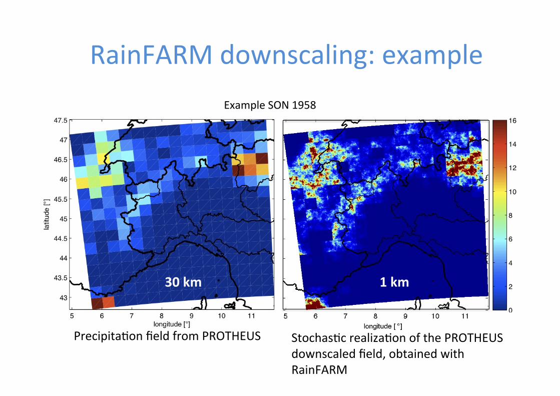
RainFARM downscaling: example
30 km 1 km
PrecipitaOon field from PROTHEUS StochasOc realizaOon of the PROTHEUS downscaled field, obtained with RainFARM
* D'Onofrio, D.; Palazzi, E.; von Hardenberg, J., Provenzale A., Calman< S.; Stochas<c Rainfall Downscaling of Climate Models. J of Hydrometeorology 15 (2), 830-‐843 (2014)
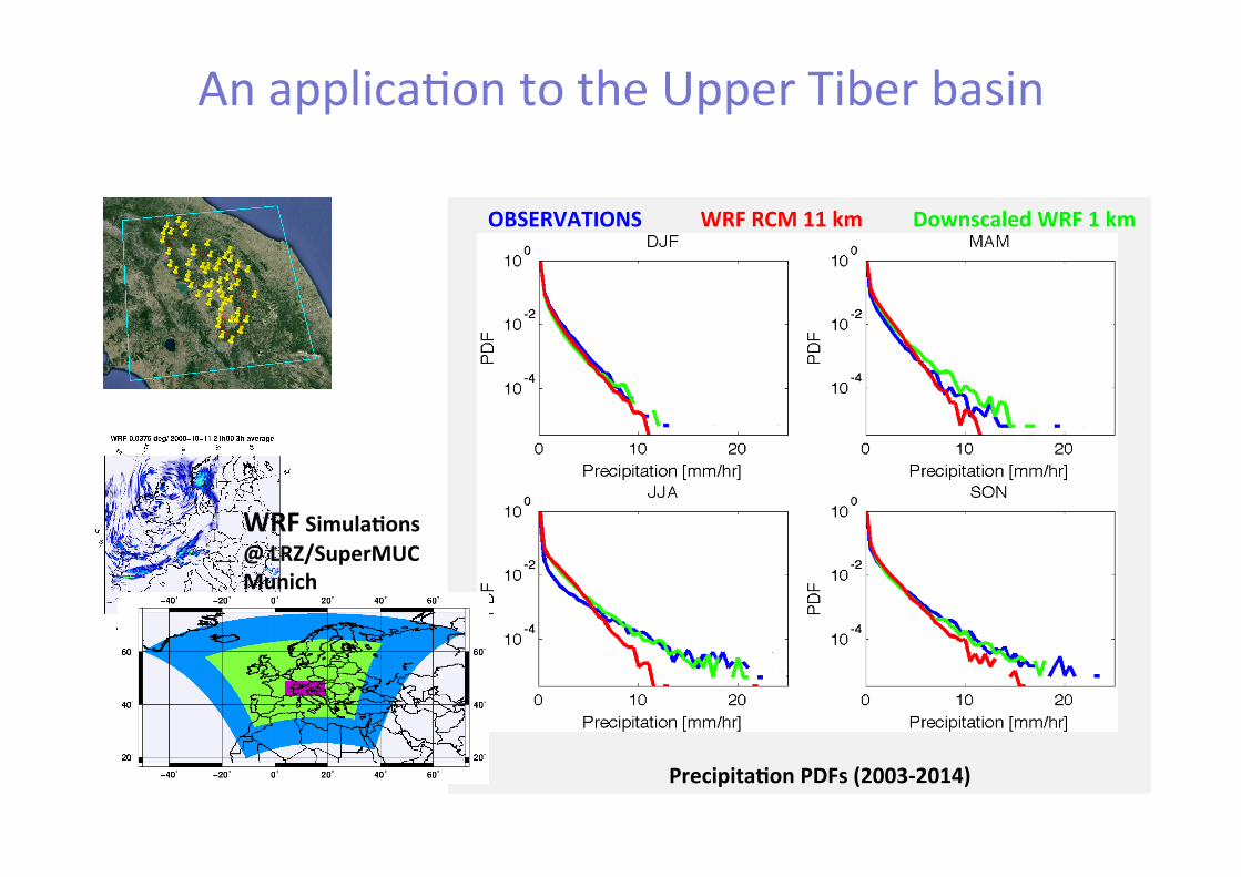
OBSERVATIONS WRF RCM 11 km Downscaled WRF 1 km
Precipita(on PDFs (2003-‐2014)
WRF Simula(ons @ LRZ/SuperMUC Munich
An applicaOon to the Upper Tiber basin
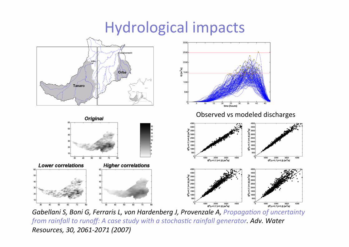
Hydrological impacts
Observed vs modeled discharges
Gabellani S, Boni G, Ferraris L, von Hardenberg J, Provenzale A, Propaga<on of uncertainty from rainfall to runoff: A case study with a stochas<c rainfall generator. Adv. Water Resources, 30, 2061-‐2071 (2007)
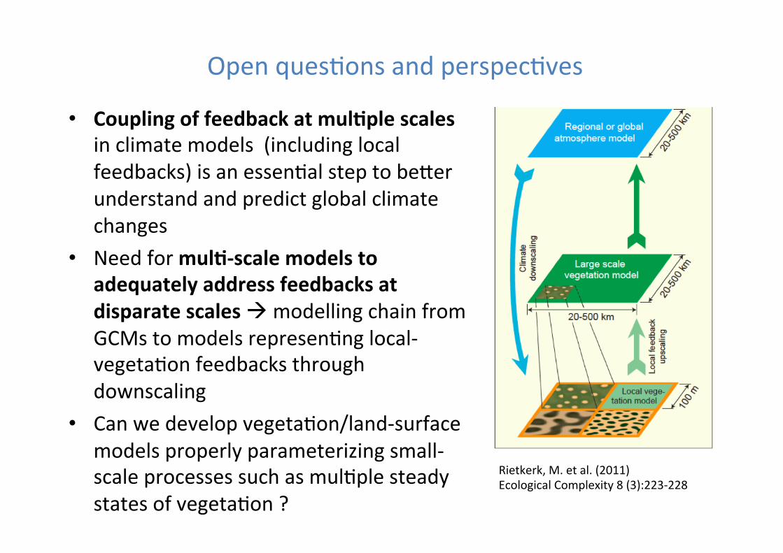
Open quesOons and perspecOves
• Coupling of feedback at mul(ple scales in climate models (including local feedbacks) is an essenOal step to be^er understand and predict global climate changes
• Need for mul(-‐scale models to adequately address feedbacks at disparate scales à modelling chain from GCMs to models represenOng local-‐vegetaOon feedbacks through downscaling
• Can we develop vegetaOon/land-‐surface models properly parameterizing small-‐scale processes such as mulOple steady states of vegetaOon ?
Rietkerk, M. et al. (2011) Ecological Complexity 8 (3):223-‐228
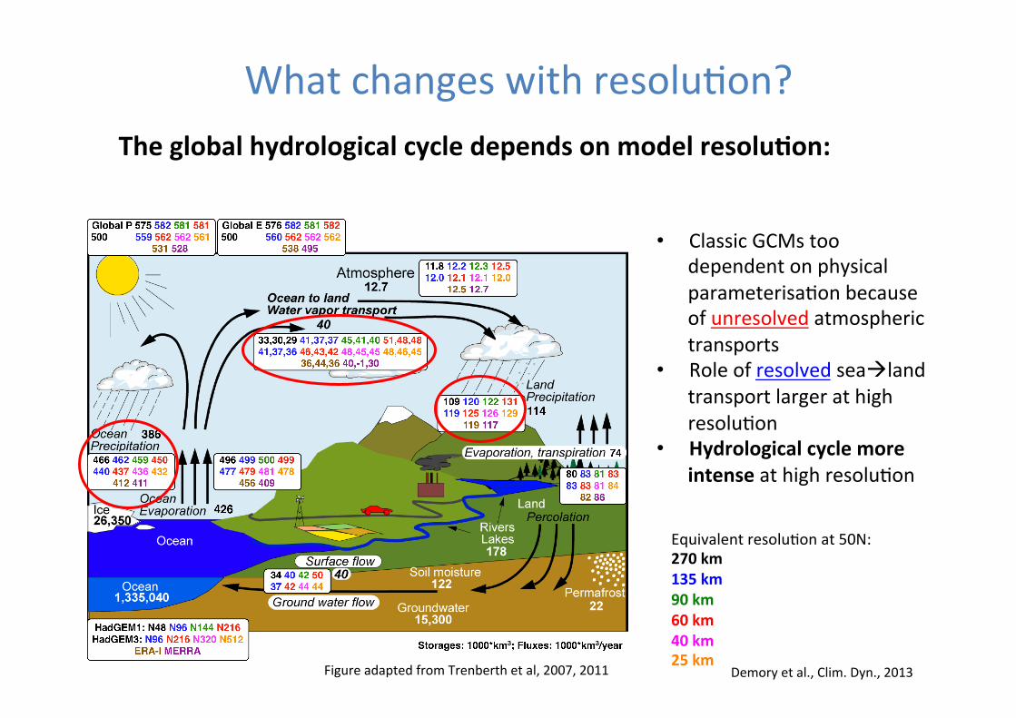
Equivalent resoluOon at 50N: 270 km 135 km 90 km 60 km 40 km 25 km
• Classic GCMs too dependent on physical parameterisaOon because of unresolved atmospheric transports
• Role of resolved seaàland transport larger at high resoluOon
• Hydrological cycle more intense at high resoluOon
What changes with resoluOon? The global hydrological cycle depends on model resolu(on:
Figure adapted from Trenberth et al, 2007, 2011 Demory et al., Clim. Dyn., 2013
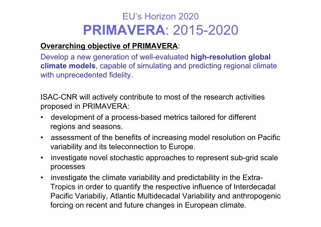
EU’s Horizon 2020 PRIMAVERA: 2015-2020
Overarching objective of PRIMAVERA: Develop a new generation of well-evaluated high-resolution global climate models, capable of simulating and predicting regional climate with unprecedented fidelity. ISAC-CNR will actively contribute to most of the research activities proposed in PRIMAVERA: • development of a process-based metrics tailored for different
regions and seasons. • assessment of the benefits of increasing model resolution on Pacific
variability and its teleconnection to Europe. • investigate novel stochastic approaches to represent sub-grid scale
processes • investigate the climate variability and predictability in the Extra-
Tropics in order to quantify the respective influence of Interdecadal Pacific Variabiliy, Atlantic Multidecadal Variability and anthropogenic forcing on recent and future changes in European climate.
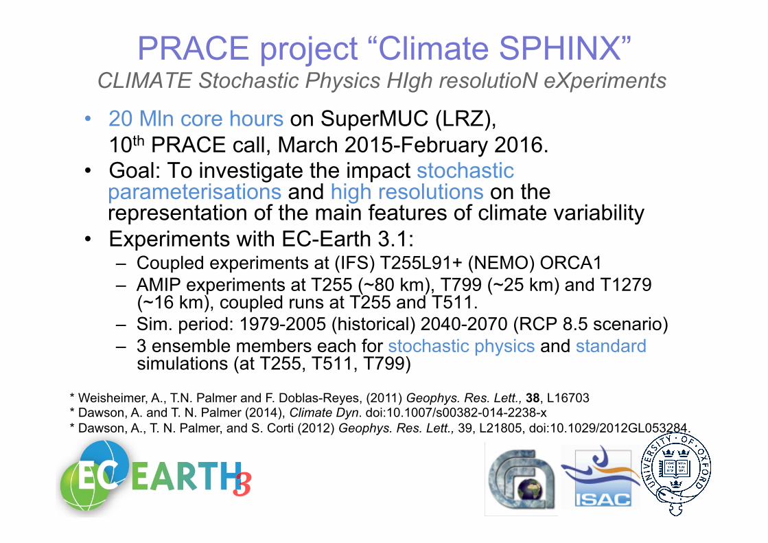
PRACE project “Climate SPHINX” CLIMATE Stochastic Physics HIgh resolutioN eXperiments
• 20 Mln core hours on SuperMUC (LRZ), 10th PRACE call, March 2015-February 2016. • Goal: To investigate the impact stochastic
parameterisations and high resolutions on the representation of the main features of climate variability
• Experiments with EC-Earth 3.1: – Coupled experiments at (IFS) T255L91+ (NEMO) ORCA1 – AMIP experiments at T255 (~80 km), T799 (~25 km) and T1279
(~16 km), coupled runs at T255 and T511. – Sim. period: 1979-2005 (historical) 2040-2070 (RCP 8.5 scenario) – 3 ensemble members each for stochastic physics and standard
simulations (at T255, T511, T799)
* Weisheimer, A., T.N. Palmer and F. Doblas-Reyes, (2011) Geophys. Res. Lett., 38, L16703 * Dawson, A. and T. N. Palmer (2014), Climate Dyn. doi:10.1007/s00382-014-2238-x * Dawson, A., T. N. Palmer, and S. Corti (2012) Geophys. Res. Lett., 39, L21805, doi:10.1029/2012GL053284.
ISAC-‐CNR will contribute in CRESCENDO to: • improvement of the land surface component of the EC-‐
Earth model, in parOcular the representaOon of ecosystem mulO-‐stability, including fire disturbances and transiOons from forest to savannah in tropical and subtropical regions.
• invesOgate impacts of land hydrology on climate (including vegetaOon-‐mediated effects) in LS3MIP experiments
• using simple process models nested in the outputs of the ESM runs as diagnosOc tools
EU’s Horizon 2020 CRESCENDO: 2015-2020
Overarching objec(ve of CRESCENDO: Improve the process realism and future projecOon reliability of European Earth-‐System Models, while evaluaOng and documenOng the performance quality of these models …