18 Triaxial Tests in Clay Introduction In Chapters 15 and 16, some aspects of the shear strength for soil were discussed. The triaxial compression test is a more sophisticated test procedure for determining the shear strength of soil. In general, with triaxial equipment, three types of common tests can be conducted, and they are listed below. Both the unconsolidated-undrained test and the consolidated-undrained test will be described in this Unconsolidated-undrained (U-U) Consolidated-drained (C-D) Consolidated-undrained (C-U) C u = undrained cohesion c = cohesion <I> = drained angle of friction A = pore water pressure parameter cu(<I> = 0) c, <I> c, <1>, A Note: s = c + 0' tab <I> (c = cohesion, 0' = effective normal stress). For undrained condition, <I> = 0; s = C u [Eq. (16.2)] Equipment 1. Triaxial cell 2. Strain-controlled compression machine 3. Specimen trimmer 4. Wire saw 5. Vacuum source 6. Oven 129
Transcript
18 Triaxial Tests in Clay
Introduction In Chapters 15 and 16, some aspects of the shear strength for soil were discussed. The triaxial compression test is a more sophisticated test procedure for determining the shear strength of soil. In general, with triaxial equipment, three types of common tests can be conducted, and they are listed below. Both the unconsolidated-undrained test and the consolidated-undrained test will be described in this ch~lptt~r.
Triaxial Cell and Loading Arrangement . Figure 18-1 shows the schematic diagram of a triaxial celt. It consists mainly of a bottom base plate, a Lucite cylinder and a top cover plate. A bottom platen is attached to the base plate. A porous stone is placed over the bottom platen, over which the soil specimen is placed. A porous stone and a platen are placed on top of the specimen. The specimen is enclosed inside a thin rubber membrane. Inletand outlet tubes for specimen saturation and drainage are provided through the base plate. Appropriate valves to these tubes are attached to shut off the openings when desired. There is an opening in the base plate through which
Soil Mechanics Laboratory Manual 1 31
water (or glycerine) can be allowed to flow to fill the cylindrical chamber. A hydrostatic chamber pressure, 03, can be applied to the specimen through the chamber fluid. Ah added axial stress, D.o, applied to the top of the specimen can be provided using a piston.
During the test, the triaxial cell is placed on the platfonn of a strain-controlled compression machine. The top of the piston of the triaxial chamber is attached to a proving ring. The proving ring is attached to a crossbar that is fixed to two metal posts. The platfonn of the compression machine can be raised (or lowered) at desired rates, thereby raising (or lowering) the triaxial cell. During compression, the load on the specimen can be obtained from the proving ring readings and the corresponding specimen defonnation from a dial gauge [1 small div. = 0.001 in. (0.0254 mm)].
The connections to the soil specimen can be attached to a burette or a pore-water pressure measuring device to measure, respectively, the volume change of the specimen or the excess pore water pressure during the test.
Triaxial equipment is costly, depending on the accessories attached to it. For that reason, general procedures for tests will be outlined here. For detailed location of various components of the assembly, students will need the help of their instructor.
Triaxial Specimen Triaxial specimens most commonly used are about 2.8 in. in diameter x 6.5 in. in length (71.1 mm diameter x 165.1 mm length) or 1.4 in. in diameter x 3.5 in. in length (35.6 mm diameter x 88.9 length). In any case, the length-to-diameter ratio (LID) should be between 2 and 3. For tests on undisturbed natural soil samples collected in shelby tubes, a specimen trimmer may need to be used to prepare a specimen of desired dimensions. Depending on the triaxial cell at hand, for classroom use, remolded specimens can be prepared with Harvard miniature compaction equipment.
After the specimen is prepared, obtain its length (Lo) and diameter (~). The length should be measured four times about 90 degrees apart. The average of these four values should be equal to Lo. To obtain the diameter, take four measurements at the top, four at the middle and four at the bottom of the specimen. The average of these twelve measurements is Do.
Placement of Specimen in the Triaxial Cell I. Boil the two porous stones to be used with the specimen. 2. De-air the lines connecting the base of the triaxial cell. 3. Attach the bottom platen to the base of the cell. 4. Place the bottom porous stone (moist) over the bottom platen .. 5. Take a thin rubber membrane of appropriate size to fit the specimen snugly. Take a
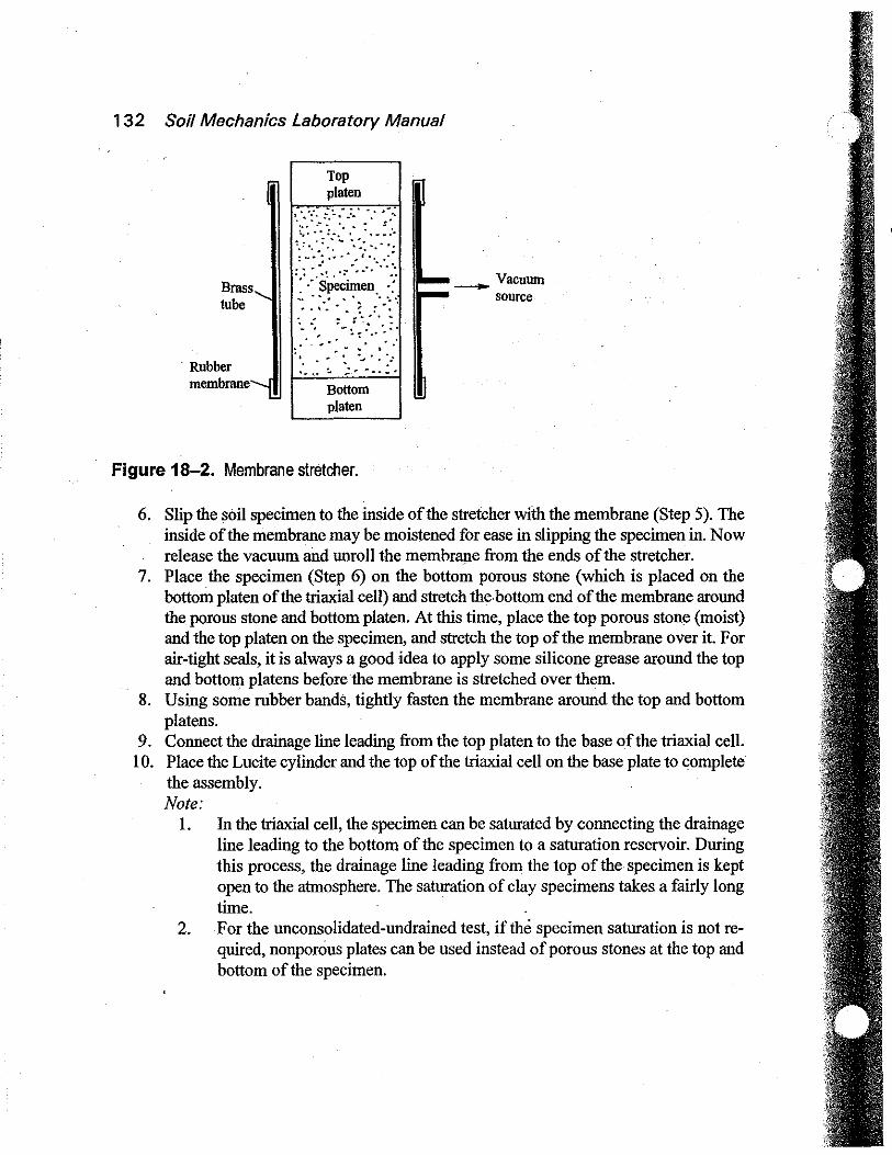
membrane stretcher, which is a brass tube with an inside diameter of about V. in. (" 6 mm) larger than the specimen diameter (Figure 18-2). The membrane stretcher can be connected to a vacuum source. Fit the membrane to the inside ofthe membrane stretcher and lap the ends of the membrane over the stretcher. Then apply the vacuum. This will make the membrane fonn a smooth cover inside the stretcher.
132 Soil Mechanics Laboratory Manual
Brass, tube
Top platen
,. ~.. .
..... __ Vacuum
~ source
Rubber membrane'-.....j
.. : ...... :: ,,,,,:' ; .. ~.-
Bottom platen
Figure 18-2. Membrane stretcher.
6. Slip the soil specimen to the inside of the stretcher with the membrane (Step 5). The inside of the membrane may be moistened for ease in slipping the specimen in. Now release the vacuum and unroll the membrane from the ends of the stretcher.
7. Place the specimen (Step 6) on the bottom porous stone (which is placed on the bottom platen of the triaxial cell) and stretch the.bottom end of the membrane around the porous stone and bottom platen. At this time, place the top porous stone (moist) and the top platen on the specimen, and stretch the top of the membrane over it. For air-tight seals, it is always a good idea to apply some silicone grease around the top and bottom platens before the membrane is stretched over them.
8. Using some rubber bands, tightly fasten the membrane around the top and bottom platens.
9. Connect the drainage line leading from the top platen to the base of the triaxial cell. 10. Place the Lucite cylinder and the top of the triaxial cell on the base plate to complete
the assembly. Note:
1.
2.
In the triaxial cell, the specimen can be saturated by connecting the drainage line leading to the bottom of the specimen to a saturation reservoir. During this process, the drainage line leading from the top of the specimen is kept open to the atmosphere. The saturation of clay specimens takes a fairly long time. For the unconsolidated-undrained test, if the specimen saturation is not required, nonporous plates can be used instead of porous stones at the top and bottom of the specimen.
Soil Mechanics Laboratory Manual 1 33
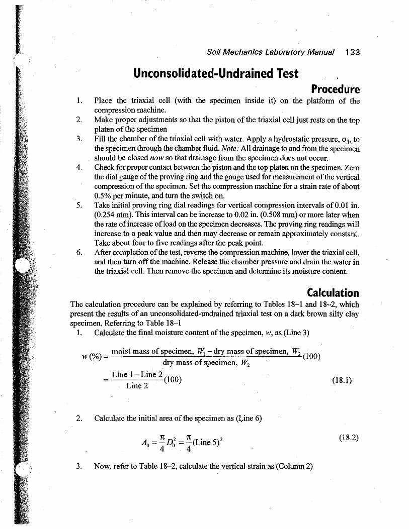
Unconsolidated-Undrained Test Procedure
1. Place the triaxial cell (with the specimen inside it) on the platfonn of the compression machine.
2. Make proper adjustments so that the piston of the triaxial cell just rests on the top platen of the specimen
3. Fill the chamber of the triaxial cell with water. Apply a hydrostatic pressure, 03'. to the specimen through the chamber fluid. Note: All drainage to and from the specimen should be closed now so that drainage from the specimen does not occur.
4. Check for proper contact between the piston and the top platen on the specimen. Zero the dial gauge of the proving ring and the gauge used for measurement of the vertical compression of the specimen. Set the compression machine for a strain rate of about 0.5% per minute, and tum the switch on.
5. Take initial proving ring dial readings for vertical compression intervals of 0.01 in. (0.254 n1m). This interval can be increase to 0.02 in. (0.508 mm) or more later when the rate of increase ofload on the specimen decreases. The proving ring readings will increase to a peak value and then may decrease or remain approximately constant. Take about four to five readings after the peak point.
6. After completion of the test, reverse the compression machine, lower the triaxial cell, and then tum off the machine. Release the chamber pressure and drain the water in the triaxial cell. Then remove the specimen and deternline its moisture content.
Calculation The calculation procedure can be explained by referring to Tables 18-1 and 18-2, which present the results of an unconsolidated-undrained triaxial test on a dark brown silty clay specimen. Referring to Table 18-1
1. Calculate the final moisture content of the specimen, w, as (Line 3)
w (%) = moist mass of specimen, W; - d?, mass of specimen, W2 (100) dry mass of speCImen, W2
= Line I - Line 2 (100) (18.1) Line 2
2. Calculate the initial area of the specimen as (Line 6)
A - rtn2 - rt(L. 5)2 "0-- 0 -- me
4 4 (18.2)
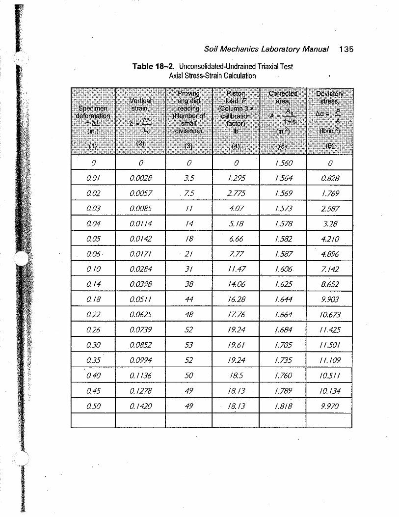
3. Now, refer to Table 18-2, calculate the vertical strain as (Column 2)
1 34 Soil Mechanics Laboratory Manual
tlL Column 1 e = - = -------Lo Line 4, Table 18-1
where AL = total deformation of the specimen at any time.
Table 18-1. Unconsolidated-Undrained Triaxial Test Preliminary Data
(18.3)
Description of SOil __ .bD.",'i1lUrk",b",l1""o""WI"",n,",,5,",i/ty;LkcJ.,,,~l...V ____ Specimen No. _.b8,--_~ __
Location __________________________ _
Tested by Date _______ _
1. Moist mass of specimen (end of test), WI 18S.68g
2. Dry mass of specimen, Wz /S/.80 g
. W,-W 3. Moisture content (end oftest), w (%) = 1 2 X 100 22.3%
W;
4. Initial average length of specimen, Lo 3.S2 in.
5. Initial average diameter of specimen, Do 1.41 in.
6. Initial area, Ao = ~ D 2 / 56 . 2 4 . tn.
7. Specific gravity of soil solids, Gs 2.73
8. Final degree of saturation 98.2%
9. Cell confining pressure, 03 IS Ibfln.2
10. Proving ring calibration factor 0.37Ib/div.
0
0.01
0.02
0.03
0.04
0.05
0.06
0.10
0.14
0.18
0.22
0.26
0.30
0.35
0.40
0.45
0.50
Soil Mechanics Laboratory Manual 135
Table 18-2. Unconsolidated-Undrained Triaxial Test Axial Stress-Strain Calculation
0 0 0 1.560
0.0028 3.5 1.295 1.564
0.0057 .7.5 2.775 1.569
0.0085 // 4.07 1.573
0.0114 14 5.18 1.578
0.0142 18 6.66 1.582
0.0171 21 7.77 1.587
0.0284 31 11.47 1.606
0.0398 38 14.06 1.625
0.051 I 44 16.28 1.644
0.0625 48 17.76 1.664
0.0739 52 19.24 1.684
0.0852 53 19.61 1.705
0.0994 52 19.24 1.735
0.//36 50 18.5 1.760
0.1278 49 18.13 1.789
0.1420 49 18.13 1.818
0
0.828
1.769
2.587
3.28
4.210
4.896
7.142
8.652
9.903
10.673
11.425
//.501
//.109
10.5//
10.134
9.970
136 Soil Mechanics Laboratory Manual
4. Calculate the piston load on the specimen (Column 4) as
P = (proving ring dial reading) x (calibration factor)
= (Column 3) x (Line 10, Table 18 -1)
5. Calculate the corrected area, A, of the specimen as (Column 5)
A = ~ = Line 6, Table 18-1 . 1- E 1 - Column 2
6. Calculate the deviatory stress (or piston stress), AU, as (Column 6)
Acr = P = Column 4 A ColumnS
Graph
(18.4)
(18.5)
(18.6)
1. Draw a graph of the axial strain (%) vs. deviatory stress (AU). As an example, the results of Table 18-2 are plotted in. Fig. 18-3. From this graph, obtain the value of Au at failure (AU = AUf).
2. The minor principal stress (total) on the specimen at failure is 03 (i.e., the chamber confining pressure). Calculate the major principal stress (total) at failure as
UI = 03 + AUf
12 _+,------------- _ l>.0/~ 11.6Ib/in.'
8
0 3 = lS1h/in.2 0, ~ 15 + 1I.6Ib/in.'
4 8 12 16 Axial strain, e (%)
Figure 18-3. Plot of l1a against axial strain for the test reported in Table 18-2.
Soil Mechanics Laboratory Manual 137
t<' .EI ~15 ~ ~
~ il lO .d
'" 5
00 10 at
20 30 Normal stress (lh/in. ')
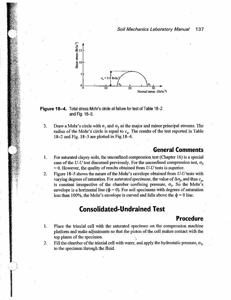
Figure 18-4. Total stress Mohr's circle at failure for test of Table 18-2 and Fig. 18-3.
3. Draw a Mohr's circle with ° I and 03 as the major and minor principal stresses. The radius of the Mohr's' circle is equal to cu' The results of the test reported in Table 18-2 and Fig. 18-3 are plotted in Fig. 18-4.
. General Comments 1. For saturated clayey soils, the unconfined compression test (Chapter 16) is a special
case of the U-U test discussed previously. For the unconfined compression test, 03
= O. However, the quality of results obtained from U-U tests is superior. 2. Figure 18-5 shows the nature of the Mohr's envelope obtained from U-Utests with
varying degrees of saturation. For saturated specimens, the value of AOp and thus cU'
is constant irrespective of the chamber confining pressure, 03' So the Mohr's envelope is a horizontal line (<I> = 0). For soil specimens with degrees of saturation less than 1 00%, the Mohr's envelope is curved and falls above the <I> = 0 line.
Consolidated-Undrained Test Procedure
1. Place the triaxial cell with the saturated specimen on the compression machine platform and make adjustments so that the piston of the cell makes contact with the top platen of the specinien.
2. Fill the chamber of the triaxial cell with water, and apply the hydrostatic pressure, 03'
to the specimen through the fluid.
1 38 Soil Mechanics Laboratory Manual
Total stress failure envelope
0 3
8 = degree of saturation 81 <82 <83
81
82
0 1 Nonna! stress
Figure 18-5. Nature of variation of total stress failure envelopes with the degree of saturation of soil specimen (for undrained test).
3. The application of the chamber pressure, 03' will cause an increase in the pore water pressure in the specimen. For consolidation connect the drainage lines from the specimen to a calibrated burette and leave the lines open. When the water level in the burette becomes constant, it will indicate that the consolidation is complete. For a saturated specimen, the volume change due to consolidation is equal to the volume of water drained from the burette. Record the volume of the drainage (AV).
4. Now connect the drainage lines to the pore-pressure measuring device. 5. Check the contact between the piston and the top platen. Zero the proving ring dial
gauge and the dial gauge, which measures the axial deformation of the specimen. 6. Set the compression machine for a strain rate of about 0.5% per minute, and turn the
switch on. When the axial load on the specimen is increased, the pore water pressure in the specimen will also increase. Record the proving ring dial gauge reading and the corresponding excess pore water pressure (Au) in the specimen for every 0.01 in. (0.254 mm) or less of axial deformation. The proving ring dial gauge reading will increase to a maximum and then decrease or remain approximately constant. Take at least four to five readings after the proving ring dial gauge reaches the maximum value.
7. At the completion of the test, reverse the compression machine and lower the triaxial cell. Shut off the machine. Release the chamber pres·sure, 03' and drain the water out of the triaxial cell.
8. Remove the tested specimen from the cell and determine its moisture content. 9. .Repeat the test on one or two more similar specimens. Each specimen should be
tested at a different value of 03.
\
I I
Soil Mechanics Laboratory Manual 139
Calculation and ~raph The procedure for making the required calculations and plotting graphs can be explained by referring to Tables IS~3 and IS--4 and Figs. IS-6 and IS-7. First, referring to Table IS-3,
1. Calculate the initial area of the specimen as (Line 5)
1t21t· 2 Ao = -Do = - (Lllle 4)
4 4
2. Calculate the initial volume of the specimen as (Line 6)
Vo = AoLo = (Line 5) x (Line 3)
3. Calculate the volume of the specimen after consolidation as (Line 9)
Ve = Vo - L'1 V = (Line 6) - (Line S)
where Ve = final volume of the specimen. 4. Calculate the length, Le (Line 10), and cross-sectional area, Ae (Line 11)
of the specimen after consolidation as
( )
1/3 1/3
Le = Lo Ve = (Line 3)(L~ne 9) Vo Lllle 6
and
( )
2/3 213
Ae = Ao Ve = (Line 5)(L~e 9) Va Lllle 6
Now refer to Table IS--4. 5. Calculate the axial strain as (Column 2)
M Column 1 E=-
Le Line 10, TablelS~3
where L'1L = axial deformation 6. Calculate the piston load, P (Column 4)
(1S.S)
(IS.9)
(IS.1 0)
(IS.11)
(IS.12)
(1S.13)
P = (proving ring dial reading, i.e. Column 3) x (calibration factor) (IS.14)
1 40 Soil Mechanics Laboratory Manual
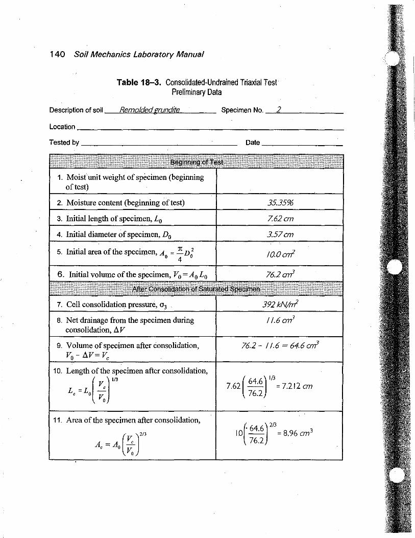
Table 18-3. Consolidated-Undrained Triaxial Test Preliminary Data
Description of soil_-,-R""e!.!.m",o",{cJ.""e~d,-<g,,,"ru,,,n,,,d,,,-1~,,,e~ __ _ Specimen No. _-,,2~ _____ _
Location ____________________________ _
Tested by ________________ _ Date_--------
1. Moisfunit weight of specimen (beginning oftest)
2. Moisture content (beginning oftest)
3. Initial length of specimen, Lo
4. Initial diameter of specimen, Do
5. Initial area of the specimen, Ao = E..D : 4
6. Initial volume of the specimen, Vo = Ao Lo
7. Cell consolidation pressure, 03
8. Net drainage from the specimen during consolidation, !:J.V
9. Volume of specimen after consolidation, Vo-!:J.V=Vc
10. Length of the specimen after consolidation,
L =L (Vc )"3 c 0 V
o
11. Area of the specimen after consolidation,
( J2/3
A =A v;, c 0 V.
o
35.35%
7.62 em
3.57em
IO.Oerrt
76.2 err?
392kN/rrt
11.6 err?
76.2 - 11.6 = 64.6 err?
7.62 ( 64.6) 1/3 = 7.212 em 76.2
10(' 64.6) 2/3 = 8.96 em3 76.2
Soil Mechanics Laboratory Manual 1 41
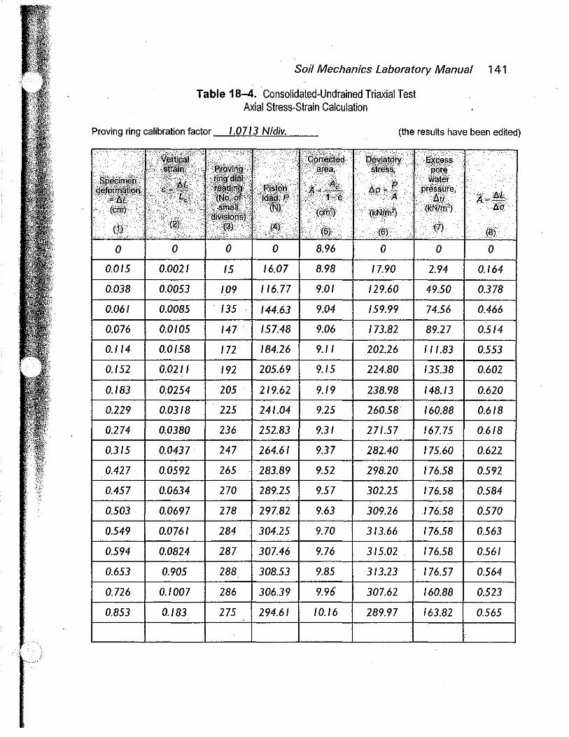
Table 18-4. Consolidated-Undrained Triaxial Test Axial Stress-Strain Calculation
Proving ring calibration factor 1.0713 Nldiv. (the results have been edited)
Figure 18-7. Effective stress Mohr's circle for remolded grundite reported in Table 18-4.
11. From the 110 vs. E (%) graph, determine the maximum Value of 110 = 110f and the corresponding values of l1u = l1uf and A = At .
In Fig. 18--6, 110f = 316 kN/m2 at E = 8.2% and, at the same strain level, l1uf= 177 kN/m2 and A = 0.56. .
12. Calculate the effective major and minor principal stresses at failure. Effective minor principal stress at failure
Effective major principal stress at failure
For the test on the remolded grundite reported in Tables 18-3 and 18-4
0;=392- 177=215kN/m2
oj"'; (392 + 316) - 177 =,531 kN/m2
(18.18)
(18.19)
13. Collect 0; and 0; for all the specimens tested and plot Mohr's circles. Plot a failure envelope that touches the Mohr's circles. The equation for the failure envelope can be given by
144 Soil Mechanics Laboratory Manual
s = c + 0' tan <I>
Detennine the values of c and <I> from the failure envelopes. Figure 18-7 shows the Mohr's circles for two tests on the remolded grundite reported in Table 18-4; (Note: The result for the Mohr's circle No.2 is not given in Table 18-4.) For the failure envelope, c = 0 and <I> = 25°. So
S = 0' tan 25°
General Comments 1. For nonnally consolidated soils, c= 0; however, for overconsolidated soils, c> O. 2. Atypical range of values of A at failure for clayey soils is given below: