i Southeast Queensland Storm Tide Response to Ex. Tropical Cyclone Oswald Reference: Report_Final.docx Date: November 2015 Mitchell Smith W0071559 Tropical Cyclone Oswald Tropical Cyclone Oswald
Transcript
i
Southeast Queensland Storm Tide Response to Ex. Tropical Cyclone Oswald Reference: Report_Final.docx Date: November 2015 Mitchell Smith W0071559 Tropical Cyclone Oswald Tropical Cyclone Oswald
ii
Abstract
Although a significant body of work exists, previous storm tide studies within Moreton Bay have consistently underestimated observed peak tide gauge levels by up to 40%. There remains scientific debate regarding the source of this “missing” contribution, which is hypothesised to be resultant from either disturbance of regional oceanic density structure, wave radiation stress gradients due to wave breaking on the Spitfire Banks or the need to improve the current parameterisation of wind stress into the water column. To support or disprove these hypotheses, this study investigates the regional surge response during the passage of Ex. Tropical Cyclone Oswald in January 2013 through the application of a series of integrated hydrodynamic and spectral wave modelling experiments. Overall, the shape and magnitude of the experiments with wave radiation stresses activated provide a better match (~27% peak underestimate) to measured residuals compared with tide plus surge only experiments (~47% underestimate) supporting the theory of wave-surge interaction. During the twenty-hour period of greatest wind speeds however, there is a consistent ~25% underestimation that tends to support a call to improve the implementation of model physics at the air-sea interface, while the effects of 3D regional ocean contributions needs to be revisited when improved model boundaries are available and this aspect cannot be dismissed.
Tropical Cyclone Oswald iii Contents
Limitations of Use
The Council of the University of Southern Queensland, its Faculty of Health, Engineering & Sciences, and the staff of the University of Southern Queensland, do not accept any responsibility for the truth, accuracy or completeness of material contained within or associated with this dissertation.
Persons using all or any part of this material do so at their own risk, and not at the risk of the Council of the University of Southern Queensland, its Faculty of Health, Engineering & Sciences or the staff of the University of Southern Queensland.
This dissertation reports an educational exercise and has no purpose or validity beyond this exercise. The sole purpose of the course pair entitled “Research Project” is to contribute to the overall education within the student’s chosen degree program. This document, the associated hardware, software, drawings, and other material set out in the associated appendices should not be used for any other purpose: if they are so used, it is entirely at the risk of the user.
Tropical Cyclone Oswald iv Contents
Candidate Certification
I certify that the ideas, designs and experimental work, results, analysis and conclusions set out in this dissertation are entirely my own efforts, except where otherwise indicated and acknowledged. I further certify that the work is original and has not been previously submitted for assessment in any other course or institution, except where specifically stated. Mitchell James Smith Student Number W0071559
2nd of November, 2015.
Tropical Cyclone Oswald v Contents
Acknowledgements
The author would like to acknowledge and thank the following for their assistance and advice during completion of the project:
Dr Md Jahangir Alam - Primary Supervisor - University of Southern Queensland
Dr Bruce Harper - External Supervisor - Systems Engineering Australia
Dr Ian Teakle - External Supervisor – BMT-WBM
Mr Toby Devlin – BMT-WBM
Dr Matthew Barnes – BMT-WBM
Dr Jason McConochie – Shell, The Hauge
Dr Dave Callaghan - University of Queensland
The author would also like to thank the on-going work of the following organisations, which without the data they collect and provide it would not have been possible to complete studies such as this.
The Queensland Department of Science, Information Technology, Innovation and the Arts;
Maritime Safety Queensland;
Manly Hydraulics Laboratory;
The Bureau of Meteorology; and
The U.S National Centre for Environmental Prediction.
Tropical Cyclone Oswald vi Contents
Contents Abstract ................................................................................................................................................ ii Limitations of Use ................................................................................................................................ iii Candidate Certification ........................................................................................................................ iv
1 Introduction ................................................................................................................ 11 1.1 Outline ............................................................................................................................... 11 1.2 The Problem ..................................................................................................................... 11 1.3 Tropical Cyclone Oswald ................................................................................................ 12 1.4 Research Objectives ........................................................................................................ 14 1.5 Report Summary .............................................................................................................. 15
2 Literature Review ....................................................................................................... 17 2.1 Physical Processes ......................................................................................................... 17
2.1.1 Introduction .................................................................................................................. 17 2.1.2 Overview of Storm Tide Components ......................................................................... 18 2.1.3 Equations of Motion ..................................................................................................... 19 2.1.4 Surface Wind and Pressure ........................................................................................ 21
2.1.4.1 Tropical Cyclones ............................................................................................................... 21 2.1.4.2 East Coast Lows ................................................................................................................. 25 2.1.4.3 Sub-Tropical, Extra-Tropical and Hybrid Systems ............................................................. 25
2.1.5 Astronomical Tide ........................................................................................................ 26 2.1.6 Bathymetry and Coastal Morphology .......................................................................... 28 2.1.7 Storm Surge ................................................................................................................ 30 2.1.8 Surface Wind Waves ................................................................................................... 30 2.1.9 Limitations in our current understanding of wave-surge physics ................................. 32 2.1.10 Ocean Vertical Structure .......................................................................................... 32 2.1.11 Oceanic Long Waves ............................................................................................... 34
2.1.12 Internal Waves ......................................................................................................... 36 2.2 Review of Recent Local Storm Tide Investigation ........................................................ 37
2.2.1 Moreton Bay and Logan/Redland Storm Tide Study ................................................... 38 2.2.2 Tropical Cyclone Rodger (Stewart, Callaghan & Nielsen 2010) .................................. 39 2.2.3 Gold Coast Storm Tide Study ...................................................................................... 40 2.2.4 Brisbane Coastal Planning and Implementation Study. .............................................. 41 2.2.5 Callaghan et al. (2012) ................................................................................................ 41
2.3 Other Relevant Literature ................................................................................................ 42
3 Research Methodology ............................................................................................. 44 4 Data Collation ............................................................................................................. 46
4.1 Bathymetry and Topography .......................................................................................... 46 4.2 Meteorological Data ......................................................................................................... 46
4.3 Gridded Ocean Data ........................................................................................................ 49 4.3.1 HYCOM ....................................................................................................................... 49 4.3.2 NOAA Wavewatch III ................................................................................................... 50 4.3.3 Astronomical Tide Model ............................................................................................. 50
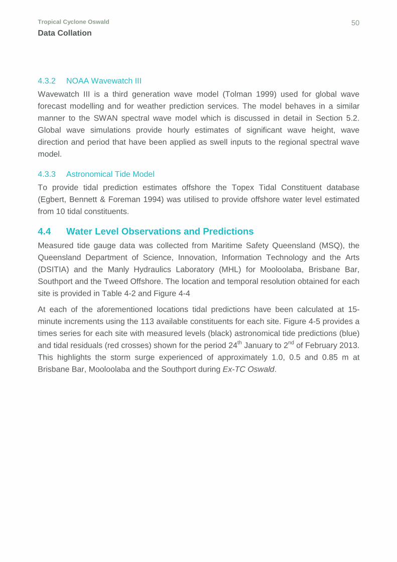
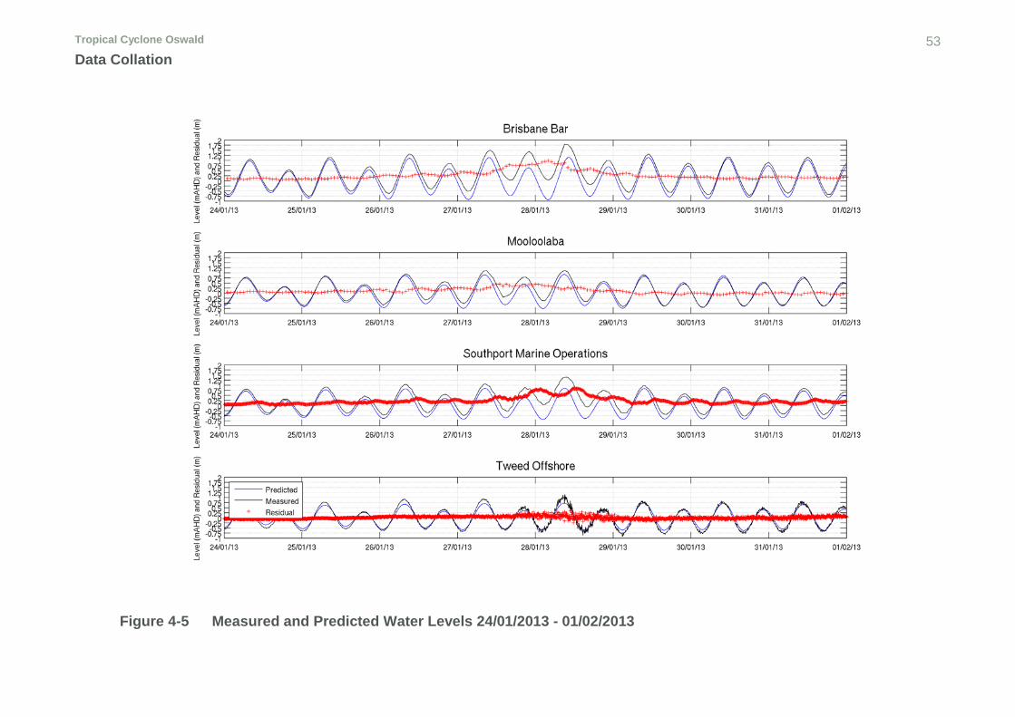
4.4 Water Level Observations and Predictions ................................................................... 50
Tropical Cyclone Oswald vii Contents
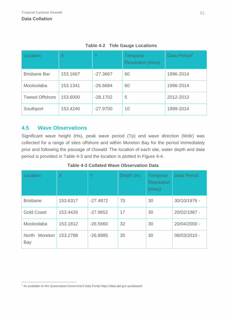
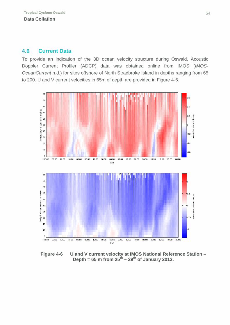
4.5 Wave Observations .......................................................................................................... 51 4.6 Current Data ..................................................................................................................... 54
5 Model Setup ............................................................................................................... 55 5.1 TUFLOW FV Hydrodynamic Model ................................................................................. 55
5.1.1 TUFLOW FV Implementation of the Non-Linear Shallow Water Equations ................ 55 5.1.2 Hydrodynamic Model Domains ................................................................................... 56 5.1.3 Simulation Period and Initial Conditions ...................................................................... 59 5.1.4 Open Boundary Conditions ......................................................................................... 59 5.1.5 Physical Parameters ................................................................................................... 60
5.2 SWAN Spectral Wave Model ........................................................................................... 60 5.2.1 Model Domains ........................................................................................................... 60 5.2.2 Open Boundary Conditions ......................................................................................... 61 5.2.3 Model Parameters ....................................................................................................... 61 5.2.4 Wave Radiation Output ............................................................................................... 61
7.2.1 Development of 3D Experiments ................................................................................. 67 7.2.2 Outcomes of 3D Experiments ..................................................................................... 68
7.3 2D Experiments ................................................................................................................ 69 7.3.1 Development of 2D Experiments ................................................................................. 69
8 Results ........................................................................................................................ 72 8.1 Method of Presentation and Analysis ............................................................................ 72 8.2 3D Model Results – Experiments 1 and 2 ...................................................................... 72 8.3 2D Model Results – HD Domain B - Experiments 3 to 5 ............................................... 73
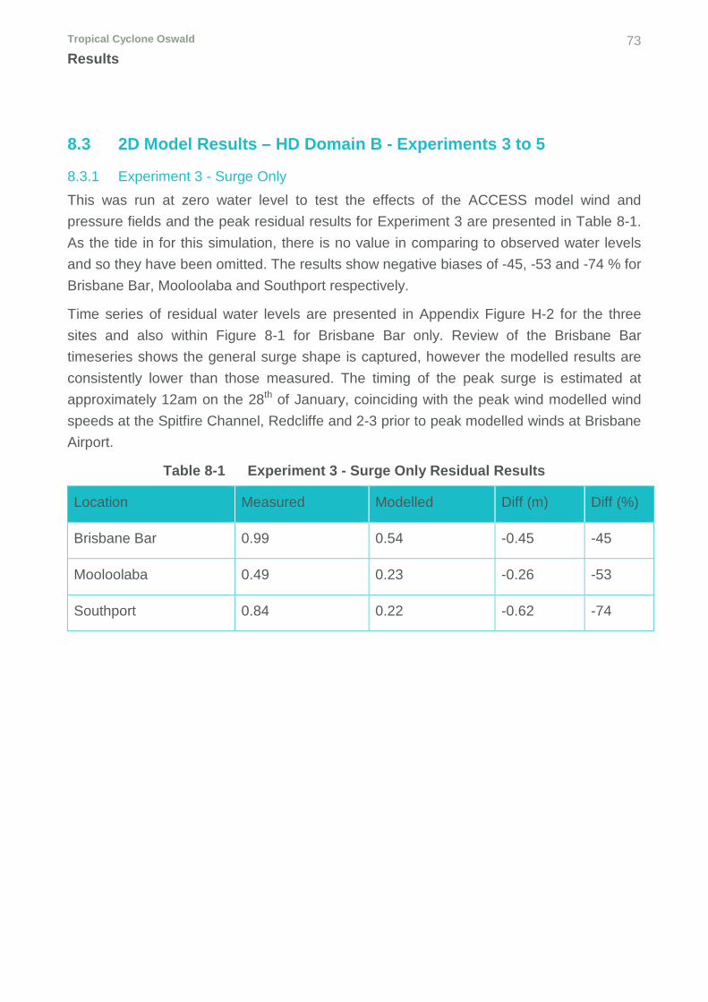
8.3.1 Experiment 3 - Surge Only .......................................................................................... 73 8.3.2 Experiment 4 - Tide plus Surge ................................................................................... 74 8.3.3 Experiment 5 - Tide plus Surge plus Waves ............................................................... 75
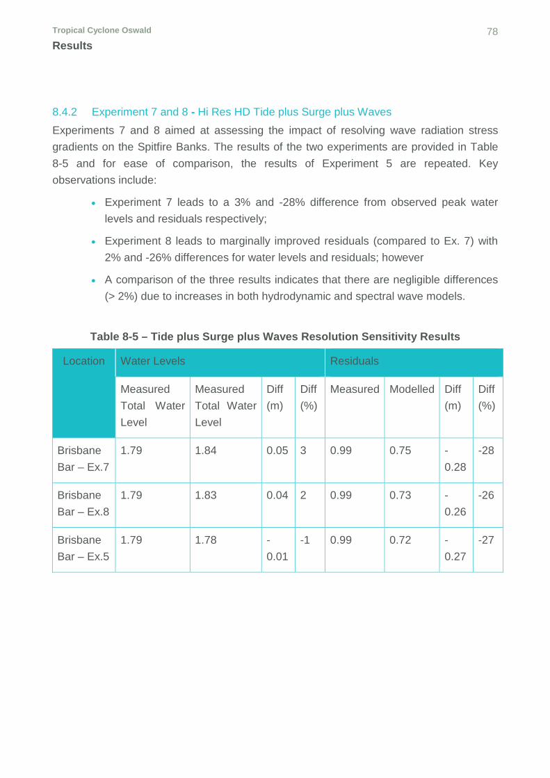
8.4 2D Model Results – HD Domain C - Experiments 6 to 8 ............................................... 77 8.4.1 Experiment 6 - Hi Res HD Tide plus Surge ................................................................. 77 8.4.2 Experiment 7 and 8 - Hi Res HD Tide plus Surge plus Waves ................................... 78
9 Discussion .................................................................................................................. 81 9.1 Study Hypothesis and Research Questions ................................................................. 81 9.2 3D Assessment ................................................................................................................ 81 9.3 Contribution of Surge, Tide and Waves at Brisbane Bar ............................................. 82 9.4 Results at Mooloolaba and Southport ........................................................................... 86 9.5 Sensitivity to Model Resolution ...................................................................................... 87 9.6 Outcomes ......................................................................................................................... 88 9.7 Implications of Research ................................................................................................ 88
10 Conclusions and Recommendations .................................................................... 90 10.1 Conclusions .................................................................................................................. 90 10.2 Limitations and Recommendations for Future Research ......................................... 92
11 References .............................................................................................................. 94 Appendix A Project Specification .................................................................................... A-1 Appendix B ACCESS Model Performance ..................................................................... B-2
Tropical Cyclone Oswald viii Contents
Appendix C Hydrodynamic Model Domains ................................................................... C-5 Appendix D TUFLOW FV Model Parameters ................................................................. D-8 Appendix E SWAN Model Parameters ......................................................................... E-11 Appendix F Model Calibration Results ......................................................................... F-13 Appendix G Experimental Total Water Level Results ................................................. G-16 Appendix H Experimental Modelled Residual Results ................................................. H-20
List of Figures Figure 1-1 Tropical Cyclone Oswald Track (Source BOM, 2013) 14
Figure 2-1 Storm Tide Components. Reproduced with permission (Harper et al. 2001) 19
Figure 2-2 Control volume force analysis for wind stress in the x direction 21
Figure 2-3 Mature Tropical Cyclone symmetrical form (left) and hybrid system (right) Source: (Bureau of Meterology n.d.)) 22
Figure 2-4 Cross section of a mature hurricane Source: (US National Weather Service n.d.) 23
Figure 2-5 Structure of Tropical Cyclone Yasi (left) and Marcia (right) approaching the Queensland coastline in 2011 and 2015 respectively (NRL, 2015). 24
Figure 2-6 Tropical Cyclones affecting the within the QLD region (left) and within 200km of Brisbane (right) for the period 1959-2006. Source: BoM, 2015b 25
Figure 2-7 Queensland Coastal Bathymetry 29
Figure 2-8 Wave setup at the shoreline (after (Hanslow & Nielsen 1992) 31
Figure 2-9 Argo ocean temperature and salinity profile and gridded sea surface temperature and sea level anomaly from IMOS. 33
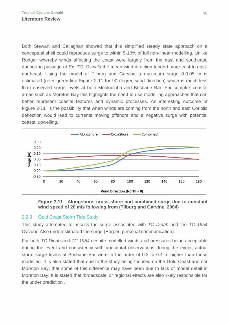
Figure 2-11 Alongshore, cross shore and combined surge due to constant wind speed of 20 m/s following from (Tilburg and Garvine, 2004) 40
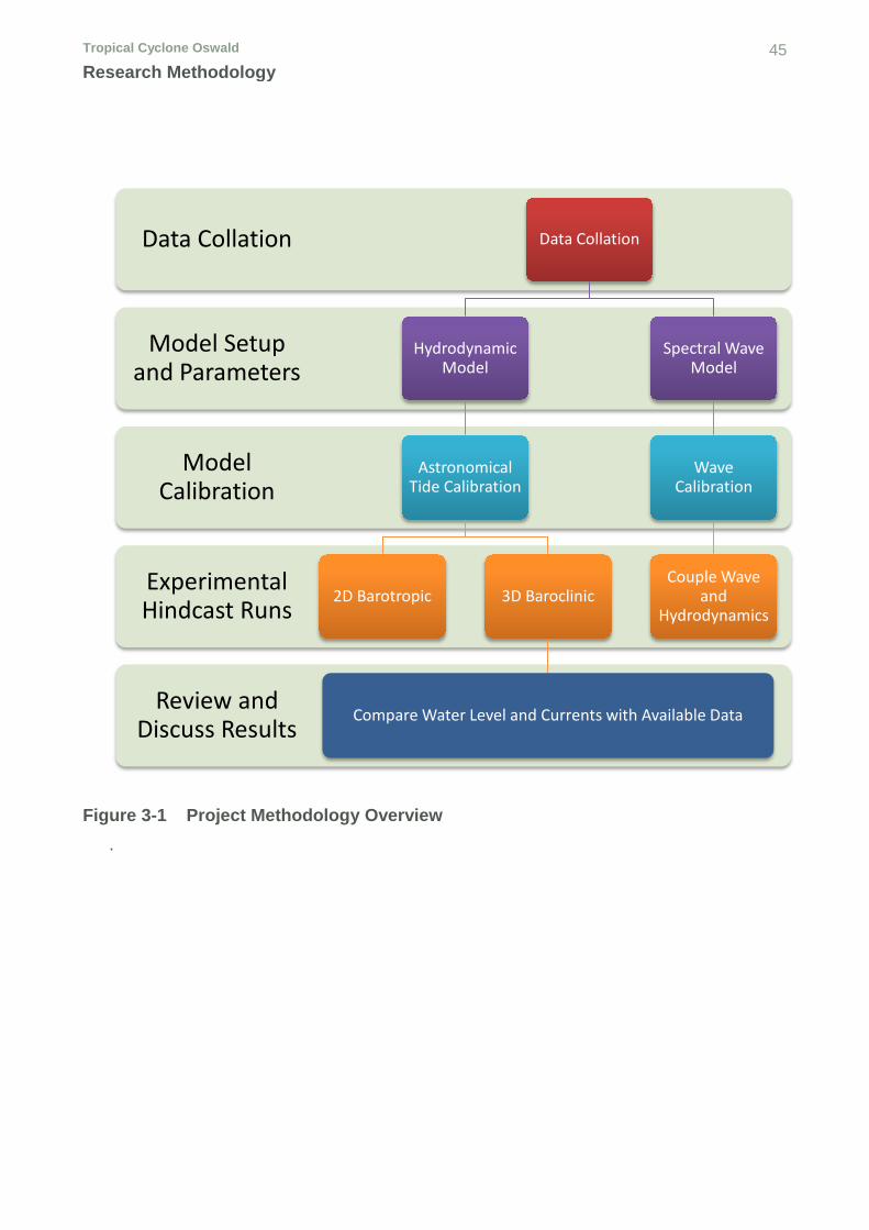
Figure 3-1 Project Methodology Overview 45
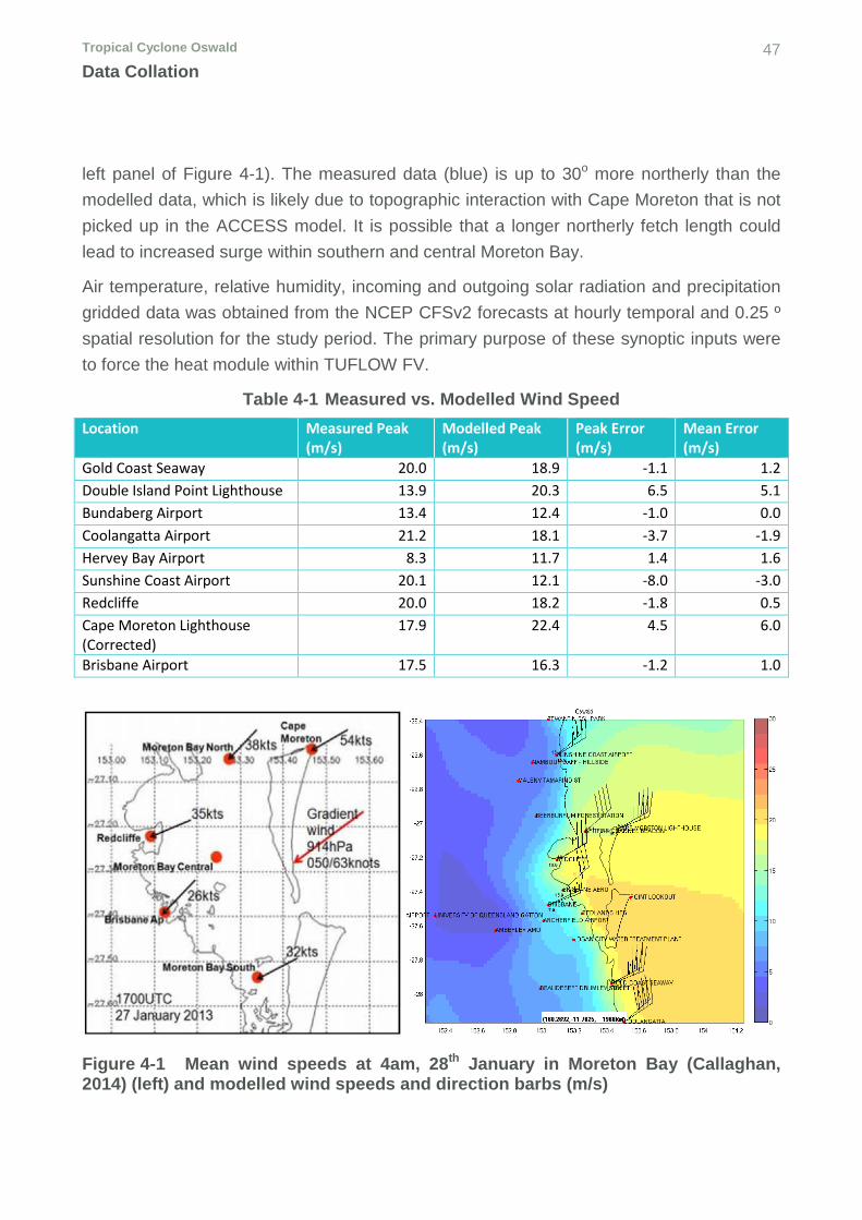
Figure 4-1 Mean wind speeds at 4am, 28th January in Moreton Bay (Callaghan, 2014) (left) and modelled wind speeds and direction barbs (m/s) 47
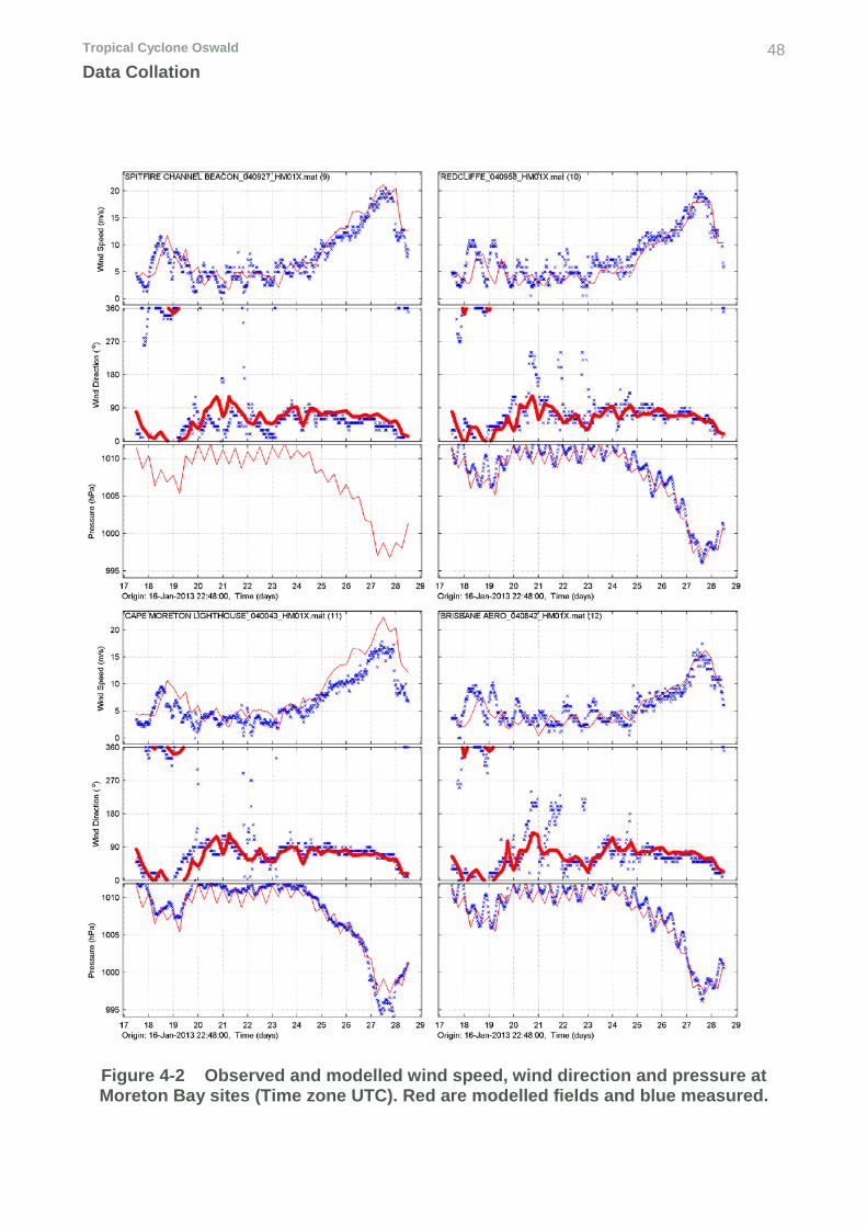
Figure 4-2 Observed and modelled wind speed, wind direction and pressure at Moreton Bay sites (Time zone UTC). Red are modelled fields and blue measured. 48
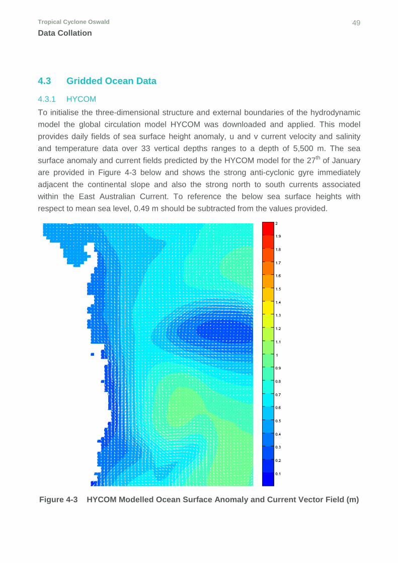
Figure 4-3 HYCOM Modelled Ocean Surface Anomaly and Current Vector Field (m) 49
Figure 4-4 Wave and Tide Gauge Locations 52
Figure 4-5 Measured and Predicted Water Levels 24/01/2013 - 01/02/2013 53
Figure 4-6 U and V current velocity at IMOS National Reference Station – Depth = 65 m from 25th – 29th of January 2013. 54
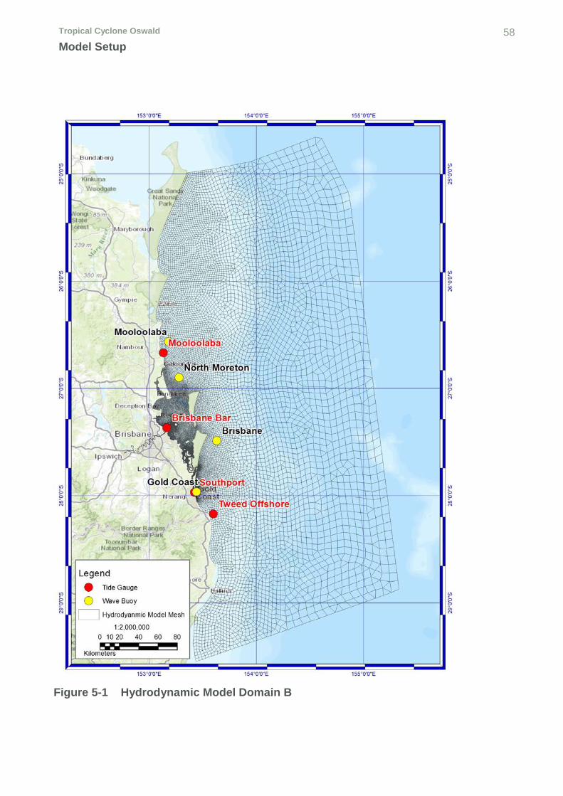
Figure 5-1 Hydrodynamic Model Domain B 58
Figure 5-2 SWAN Spectral Model Domains. RWQM (outer yellow), D001 (red), D002 (inner yellow) and E001 (black). 63
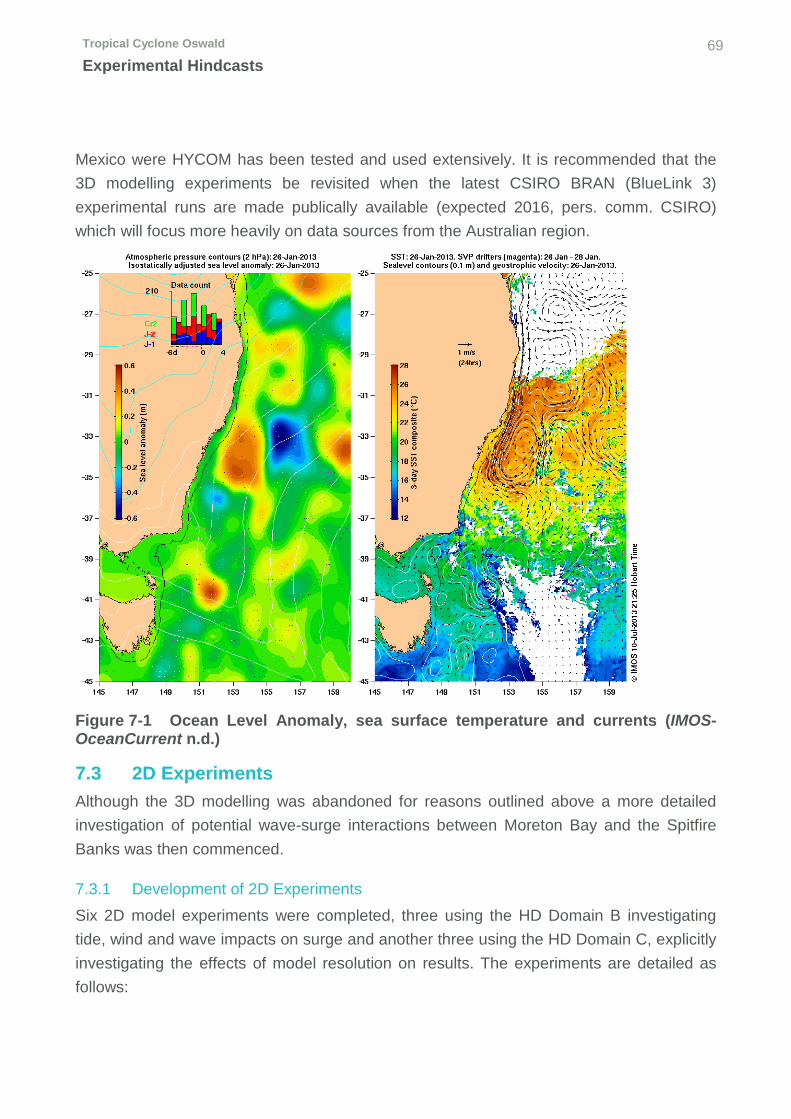
Figure 7-1 Ocean Level Anomaly, sea surface temperature and currents (IMOS-OceanCurrent n.d.) 69
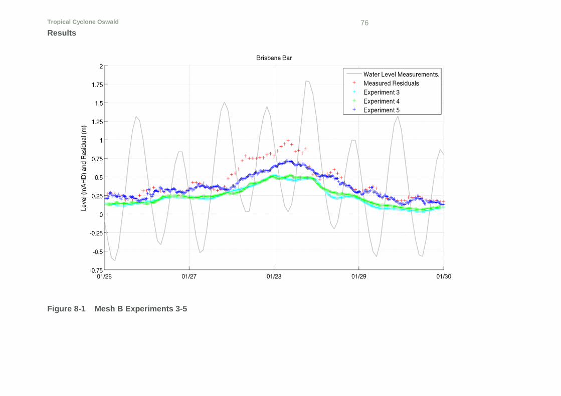
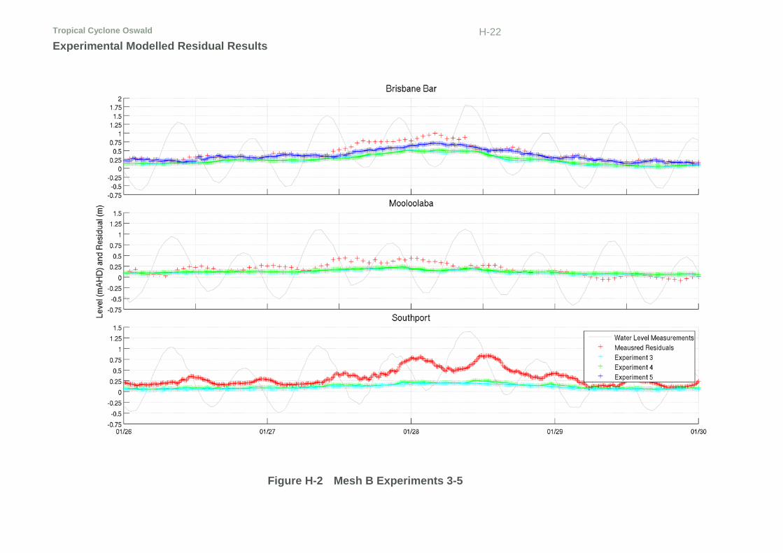
Figure 8-1 Mesh B Experiments 3-5 76
Figure 8-2 Mesh C Experiments 6-8 79
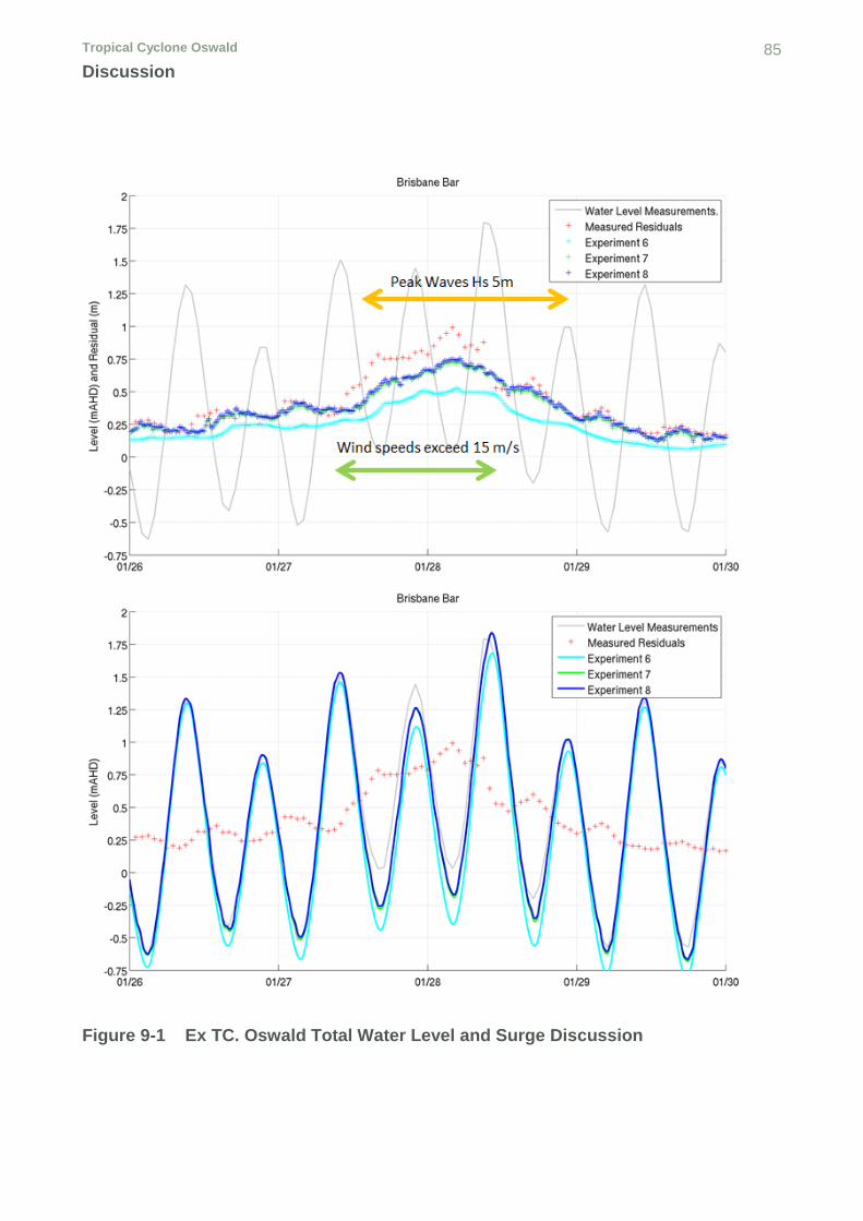
Figure 9-1 Ex TC. Oswald Total Water Level and Surge Discussion 85
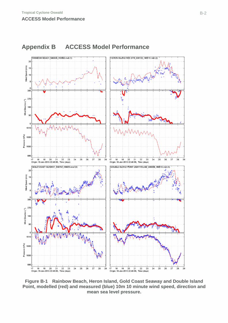
Figure B-1 Rainbow Beach, Heron Island, Gold Coast Seaway and Double Island Point, modelled (red) and measured (blue) 10m 10 minute wind speed, direction and mean sea level pressure. B-2
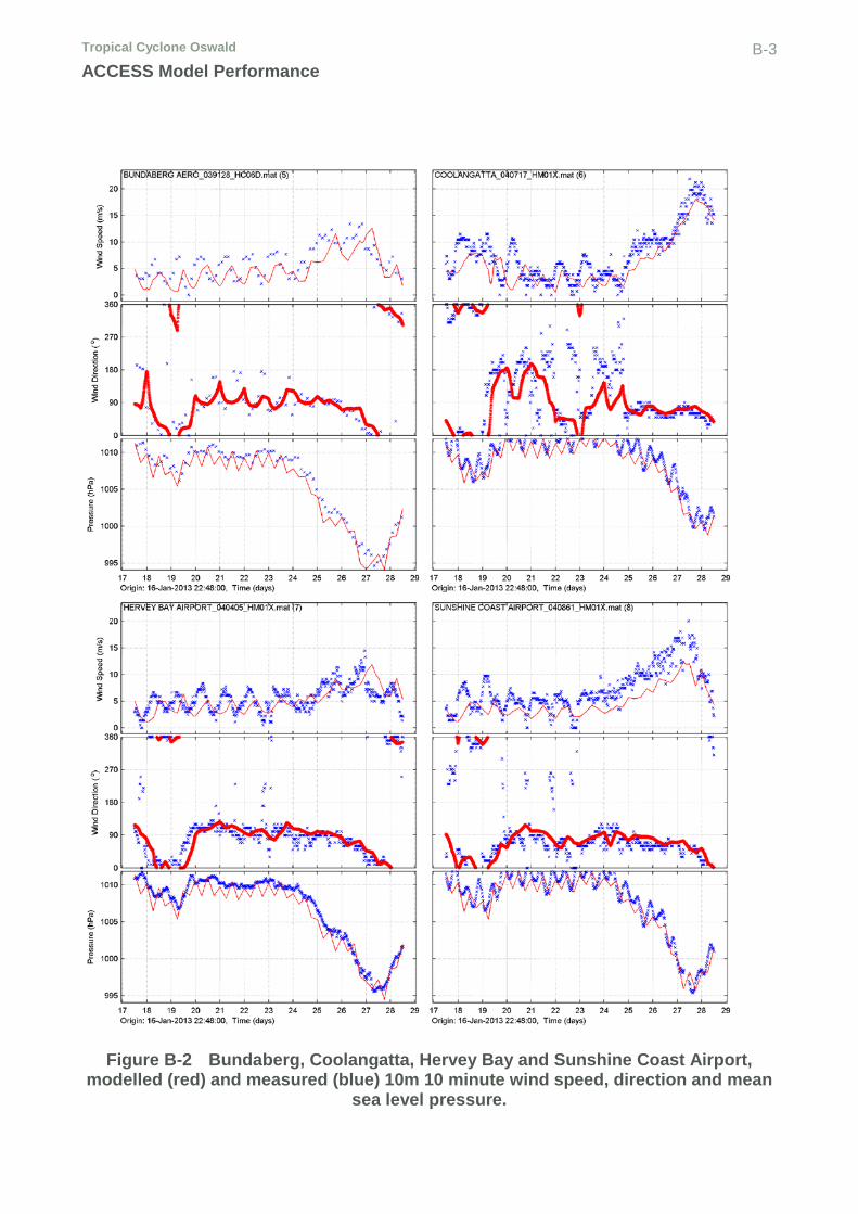
Figure B-2 Bundaberg, Coolangatta, Hervey Bay and Sunshine Coast Airport, modelled (red) and measured (blue) 10m 10 minute wind speed, direction and mean sea level pressure. B-3
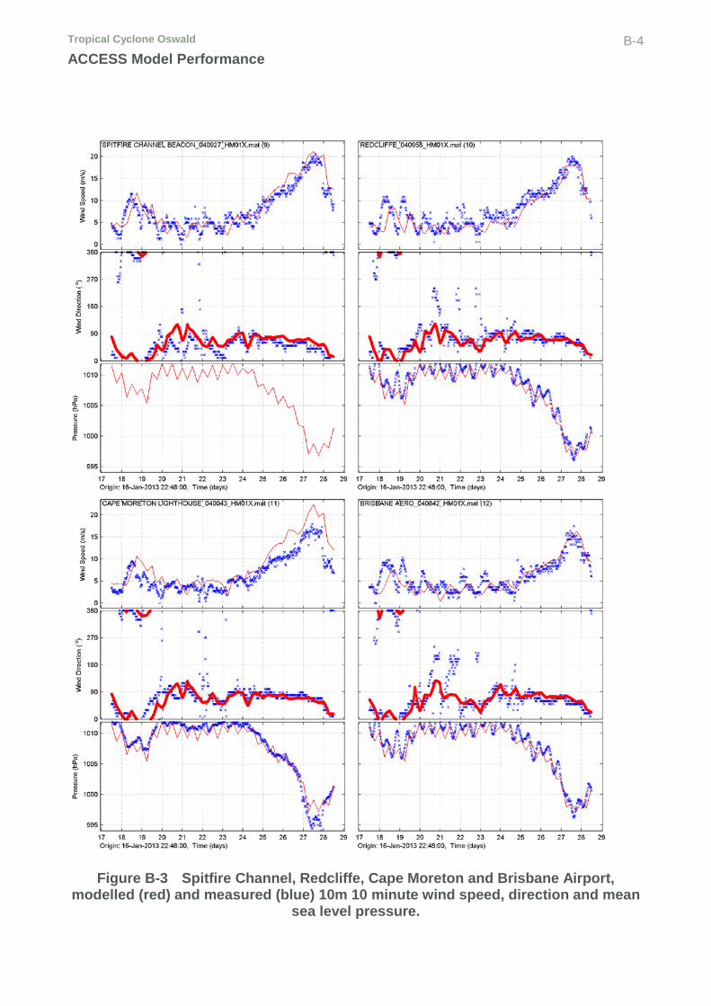
Figure B-3 Spitfire Channel, Redcliffe, Cape Moreton and Brisbane Airport, modelled (red) and measured (blue) 10m 10 minute wind speed, direction and mean sea level pressure. B-4
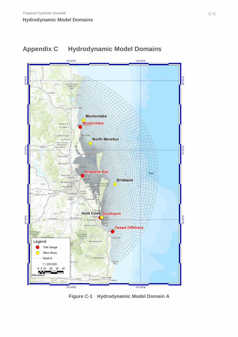
Figure C-1 Hydrodynamic Model Domain A C-5
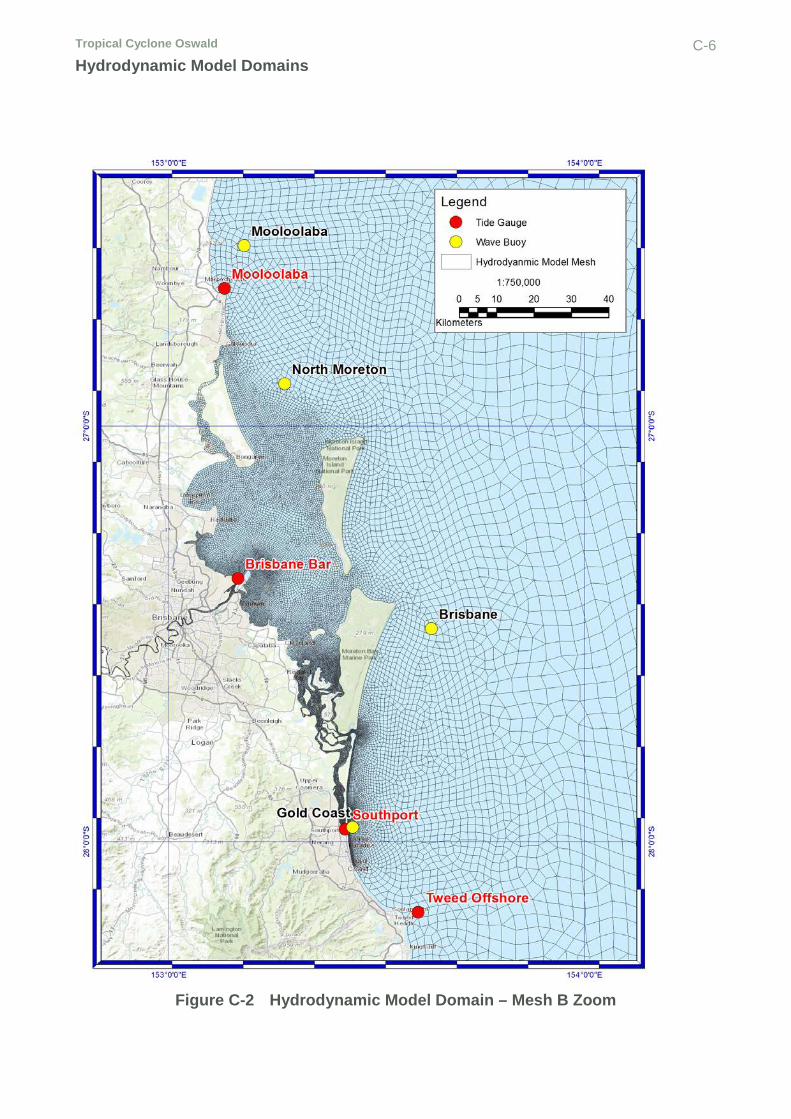
Figure C-2 Hydrodynamic Model Domain – Mesh B Zoom C-6
Figure C-3 Increased Resolution of Hydrodynamic. Domain B (top) Domain C (bottom) C-7
Figure G-1 Water Level Time-series 26/01/2013 – 01/03/2013 AEST Experiments 3, 4 and 5 at Brisbane Bar, Mooloolaba and Southport Tide Gauges G-17
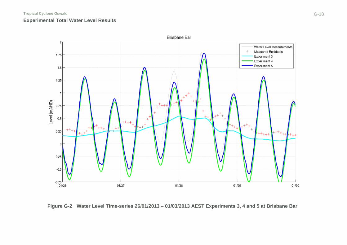
Figure G-2 Water Level Time-series 26/01/2013 – 01/03/2013 AEST Experiments 3, 4 and 5 at Brisbane Bar G-18
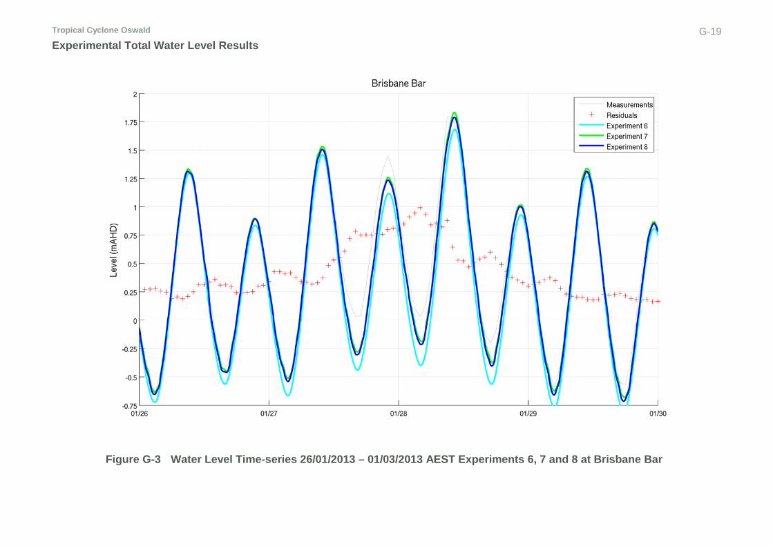
Figure G-3 Water Level Time-series 26/01/2013 – 01/03/2013 AEST Experiments 6, 7 and 8 at Brisbane Bar G-19
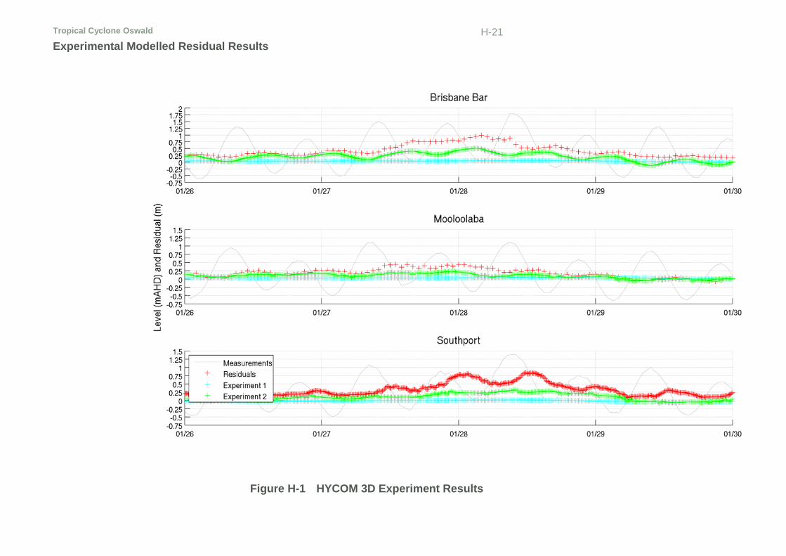
Figure H-1 HYCOM 3D Experiment Results H-21
Figure H-2 Mesh B Experiments 3-5 H-22
List of Tables Table 2-1 Tropical Cyclone Category Scale 24
Table 2-2 Brisbane Bar Tidal Constituents 27
Table 2-3 2015 Brisbane Bar Tidal Planes 27
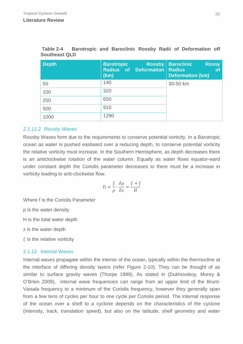
Table 2-4 Barotropic and Baroclinic Rossby Radii of Deformation off Southeast QLD 36
Table 4-1 Measured vs. Modelled Wind Speed 47
Table 4-2 Tide Gauge Locations 51
Table 4-3 Collated Wave Observation Data 51
Table 5-1 Wave Model Domains 61
Tropical Cyclone Oswald x Contents
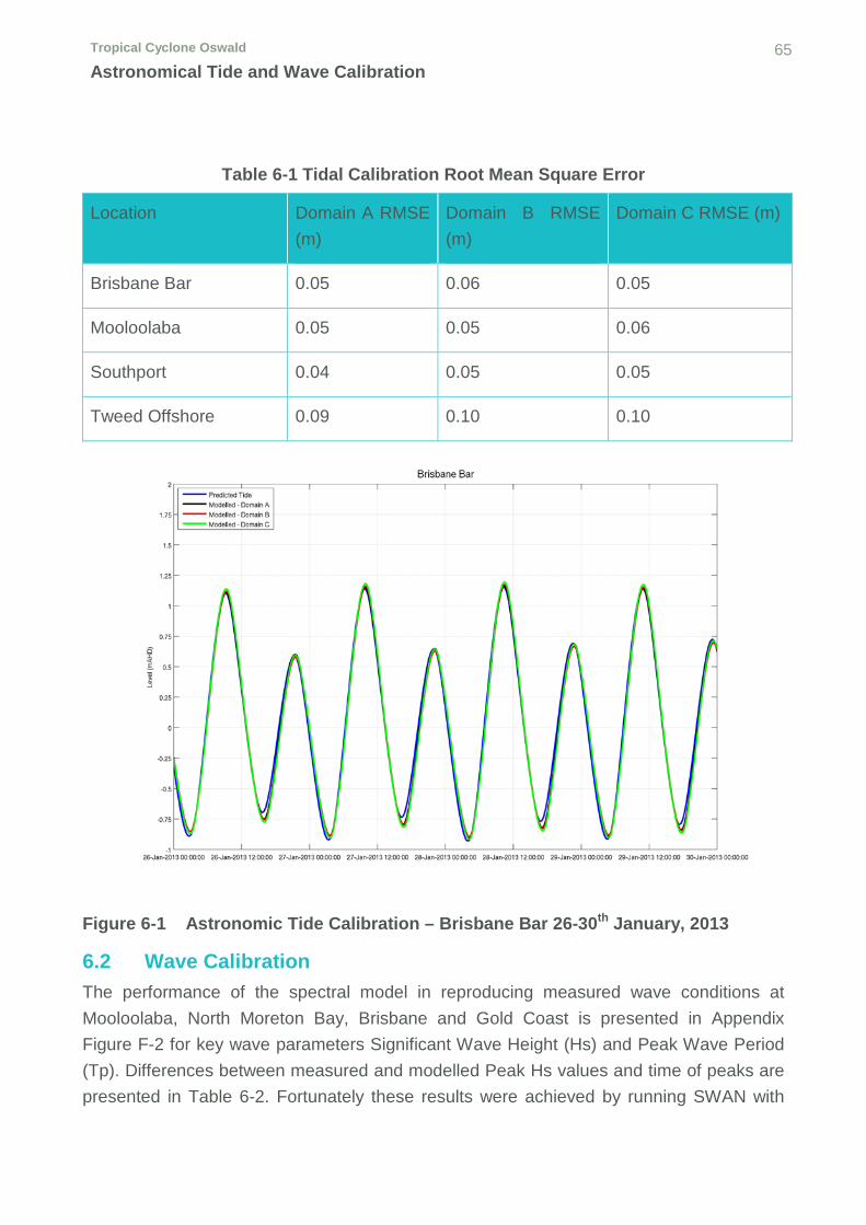
Table 6-1 Tidal Calibration Root Mean Square Error 65
Table 6-2 Measured and Modelled Peak Significant Wave Heights 66
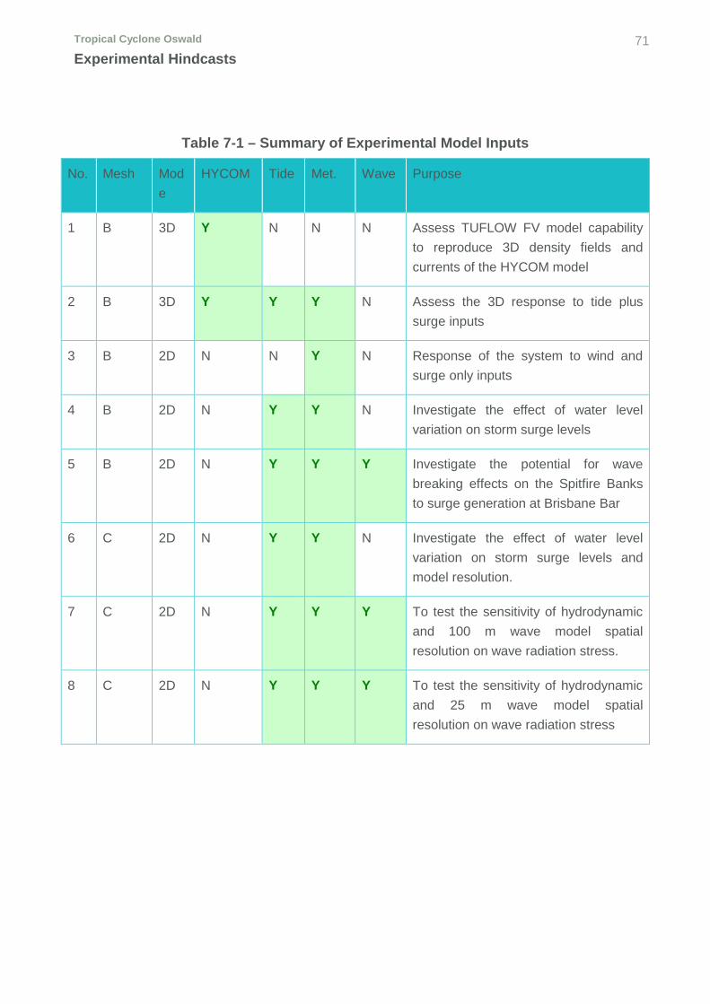
Table 7-1 – Summary of Experimental Model Inputs 71
Table 8-1 Experiment 3 - Surge Only Residual Results 73
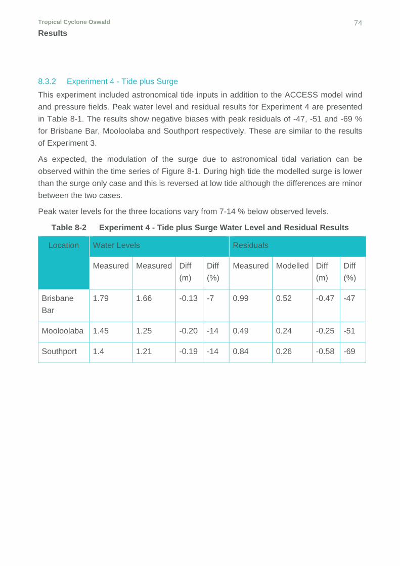
Table 8-2 Experiment 4 - Tide plus Surge Water Level and Residual Results 74
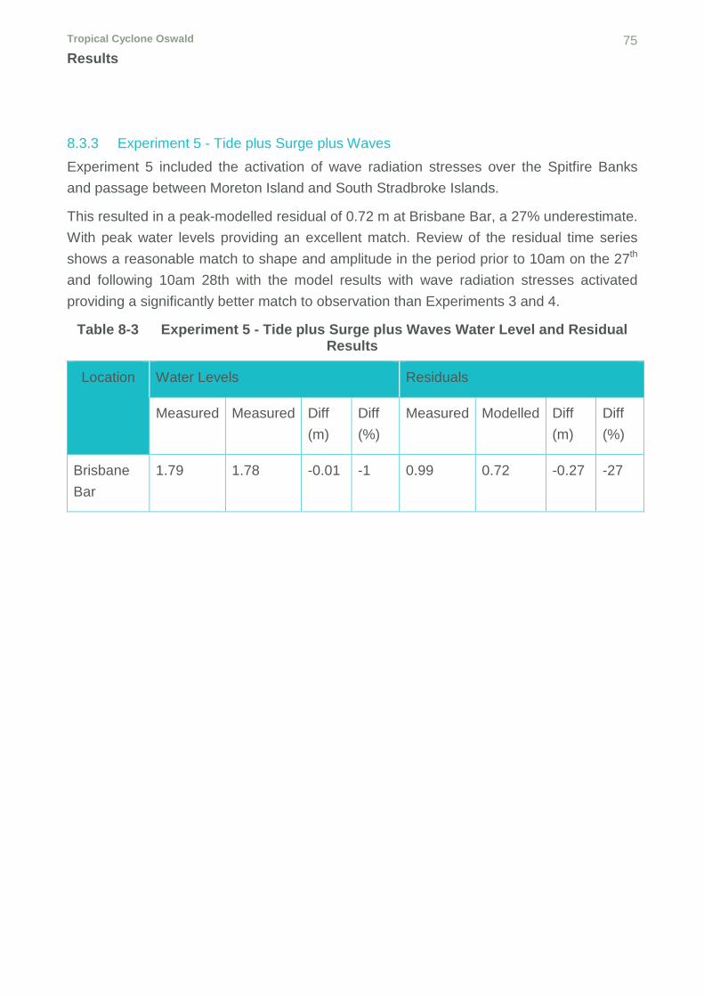
Table 8-3 Experiment 5 - Tide plus Surge plus Waves Water Level and Residual Results 75
Table 8-4 Tide plus Surge Resolution Sensitivity Results 77
Table 8-5 – Tide plus Surge plus Waves Resolution Sensitivity Results 78
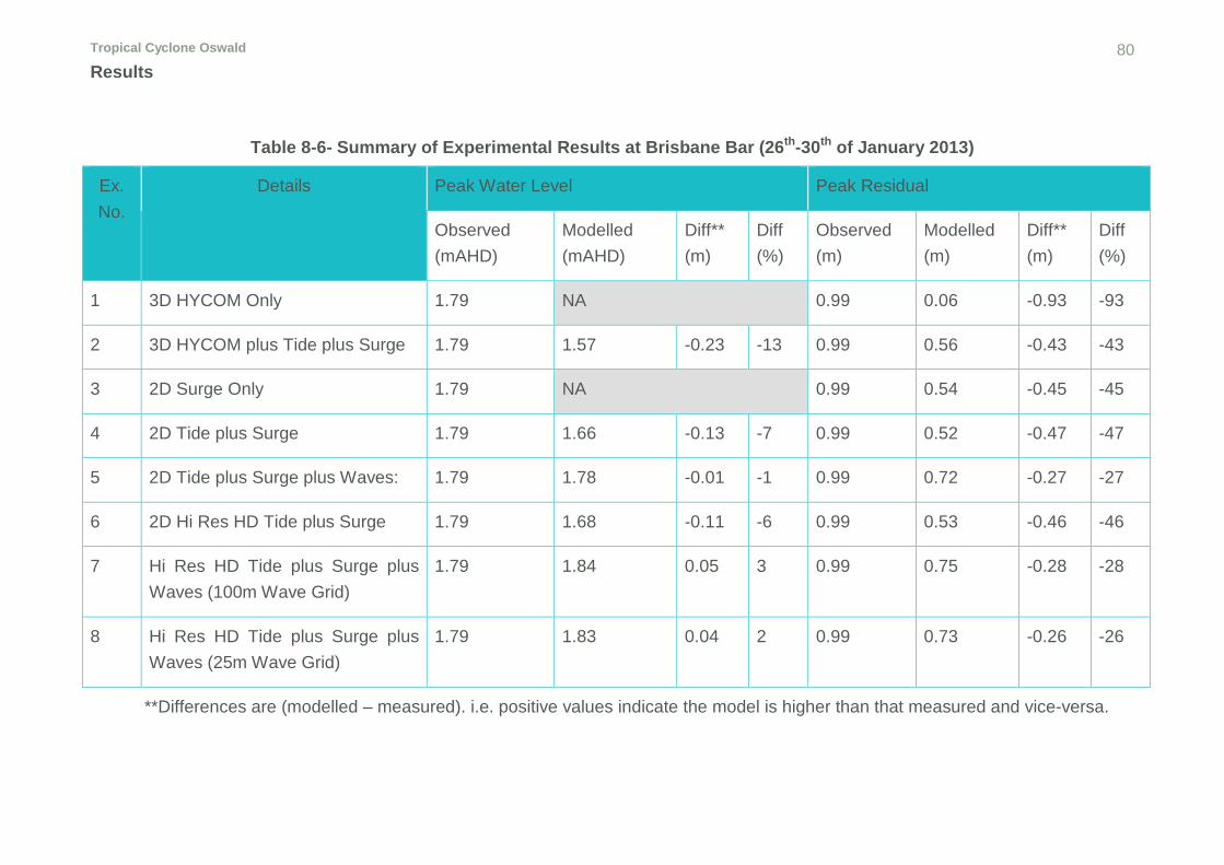
Table 8-6- Summary of Experimental Results at Brisbane Bar (26th-30th of January 2013) 80
SEQ Storm Tide Response to Ex. Tropical Cyclone Oswald ii Abstract
Abstract
Although a significant body of work exists, previous storm tide studies within Moreton Bay have consistently underestimated observed peak tide gauge levels by up to 40%. There remains scientific debate regarding the source of this “missing” contribution, which is hypothesised to be resultant from either disturbance of regional oceanic density structure, wave radiation stress gradients due to wave breaking on the Spitfire Banks or the need to improve the current parameterisation of wind stress into the water column. To support or disprove these hypotheses, this study investigates the regional surge response during the passage of Ex. Tropical Cyclone Oswald in January 2013 through the application of a series of integrated hydrodynamic and spectral wave modelling experiments. Overall, the shape and magnitude of the experiments with wave radiation stresses activated provide a better match (~27% peak underestimate) to measured residuals compared with tide plus surge only experiments (~47% underestimate) supporting the theory of wave-surge interaction. During the twenty-hour period of greatest wind speeds however, there is a consistent ~25% underestimation that tends to support a call to improve the implementation of model physics at the air-sea interface, while the effects of 3D regional ocean contributions needs to be revisited when improved model boundaries are available and this aspect cannot be dismissed.
Tropical Cyclone Oswald iii Contents
Limitations of Use
The Council of the University of Southern Queensland, its Faculty of Health, Engineering & Sciences, and the staff of the University of Southern Queensland, do not accept any responsibility for the truth, accuracy or completeness of material contained within or associated with this dissertation.
Persons using all or any part of this material do so at their own risk, and not at the risk of the Council of the University of Southern Queensland, its Faculty of Health, Engineering & Sciences or the staff of the University of Southern Queensland.
This dissertation reports an educational exercise and has no purpose or validity beyond this exercise. The sole purpose of the course pair entitled “Research Project” is to contribute to the overall education within the student’s chosen degree program. This document, the associated hardware, software, drawings, and other material set out in the associated appendices should not be used for any other purpose: if they are so used, it is entirely at the risk of the user.
Tropical Cyclone Oswald iv Contents
Candidate Certification
I certify that the ideas, designs and experimental work, results, analysis and conclusions set out in this dissertation are entirely my own efforts, except where otherwise indicated and acknowledged. I further certify that the work is original and has not been previously submitted for assessment in any other course or institution, except where specifically stated. Mitchell James Smith Student Number W0071559
2nd of November, 2015.
Tropical Cyclone Oswald v Contents
Acknowledgements
The author would like to acknowledge and thank the following for their assistance and advice during completion of the project:
Dr Md Jahangir Alam - Primary Supervisor - University of Southern Queensland
Dr Bruce Harper - External Supervisor - Systems Engineering Australia
Dr Ian Teakle - External Supervisor – BMT-WBM
Mr Toby Devlin – BMT-WBM
Dr Matthew Barnes – BMT-WBM
Dr Jason McConochie – Shell, The Hauge
Dr Dave Callaghan - University of Queensland
The author would also like to thank the on-going work of the following organisations, which without the data they collect and provide it would not have been possible to complete studies such as this.
• The Queensland Department of Science, Information Technology, Innovation and the Arts;
• Maritime Safety Queensland;
• Manly Hydraulics Laboratory;
• The Bureau of Meteorology; and
• The U.S National Centre for Environmental Prediction.
Tropical Cyclone Oswald vi Contents
Contents Abstract ................................................................................................................................................ ii Limitations of Use ................................................................................................................................ iii Candidate Certification ........................................................................................................................ iv
1 Introduction ................................................................................................................ 11 1.1 Outline ............................................................................................................................ 11 1.2 The Problem ................................................................................................................... 11 1.3 Tropical Cyclone Oswald ............................................................................................... 12 1.4 Research Objectives ...................................................................................................... 14 1.5 Report Summary ............................................................................................................ 15
2 Literature Review ....................................................................................................... 17 2.1 Physical Processes ........................................................................................................ 17
2.1.1 Introduction ................................................................................................................ 17 2.1.2 Overview of Storm Tide Components ........................................................................ 18 2.1.3 Equations of Motion ................................................................................................... 19 2.1.4 Surface Wind and Pressure ....................................................................................... 21
2.1.4.1 Tropical Cyclones ............................................................................................................... 21 2.1.4.2 East Coast Lows ................................................................................................................. 25 2.1.4.3 Sub-Tropical, Extra-Tropical and Hybrid Systems ............................................................. 25
2.1.5 Astronomical Tide ...................................................................................................... 26 2.1.6 Bathymetry and Coastal Morphology ......................................................................... 28 2.1.7 Storm Surge .............................................................................................................. 30 2.1.8 Surface Wind Waves ................................................................................................. 30 2.1.9 Limitations in our current understanding of wave-surge physics ................................ 32 2.1.10 Ocean Vertical Structure......................................................................................... 32 2.1.11 Oceanic Long Waves ............................................................................................. 34
4.3 Gridded Ocean Data ....................................................................................................... 49 4.3.1 HYCOM ..................................................................................................................... 49 4.3.2 NOAA Wavewatch III ................................................................................................. 50 4.3.3 Astronomical Tide Model ........................................................................................... 50
4.4 Water Level Observations and Predictions .................................................................. 50
Tropical Cyclone Oswald vii Contents
4.5 Wave Observations ........................................................................................................ 51 4.6 Current Data ................................................................................................................... 54
5 Model Setup ............................................................................................................... 55 5.1 TUFLOW FV Hydrodynamic Model ............................................................................... 55
5.1.1 TUFLOW FV Implementation of the Non-Linear Shallow Water Equations ................ 55 5.1.2 Hydrodynamic Model Domains .................................................................................. 56 5.1.3 Simulation Period and Initial Conditions ..................................................................... 59 5.1.4 Open Boundary Conditions ........................................................................................ 59 5.1.5 Physical Parameters .................................................................................................. 60
5.2 SWAN Spectral Wave Model.......................................................................................... 60 5.2.1 Model Domains .......................................................................................................... 60 5.2.2 Open Boundary Conditions ........................................................................................ 61 5.2.3 Model Parameters ..................................................................................................... 61 5.2.4 Wave Radiation Output .............................................................................................. 61
7.2.1 Development of 3D Experiments ............................................................................... 67 7.2.2 Outcomes of 3D Experiments .................................................................................... 68
7.3 2D Experiments .............................................................................................................. 69 7.3.1 Development of 2D Experiments ............................................................................... 69
8 Results ........................................................................................................................ 72 8.1 Method of Presentation and Analysis ........................................................................... 72 8.2 3D Model Results – Experiments 1 and 2 ..................................................................... 72 8.3 2D Model Results – HD Domain B - Experiments 3 to 5 .............................................. 73
8.3.1 Experiment 3 - Surge Only ......................................................................................... 73 8.3.2 Experiment 4 - Tide plus Surge.................................................................................. 74 8.3.3 Experiment 5 - Tide plus Surge plus Waves .............................................................. 75
8.4 2D Model Results – HD Domain C - Experiments 6 to 8 .............................................. 77 8.4.1 Experiment 6 - Hi Res HD Tide plus Surge ................................................................ 77 8.4.2 Experiment 7 and 8 - Hi Res HD Tide plus Surge plus Waves ................................... 78
9 Discussion .................................................................................................................. 81 9.1 Study Hypothesis and Research Questions ................................................................ 81 9.2 3D Assessment .............................................................................................................. 81 9.3 Contribution of Surge, Tide and Waves at Brisbane Bar ............................................ 82 9.4 Results at Mooloolaba and Southport .......................................................................... 86 9.5 Sensitivity to Model Resolution .................................................................................... 87 9.6 Outcomes ....................................................................................................................... 88 9.7 Implications of Research ............................................................................................... 88
10 Conclusions and Recommendations .................................................................... 90 10.1 Conclusions ................................................................................................................ 90 10.2 Limitations and Recommendations for Future Research ........................................ 92
11 References .............................................................................................................. 94 Appendix A Project Specification .................................................................................... A-1 Appendix B ACCESS Model Performance ..................................................................... B-2
Tropical Cyclone Oswald viii Contents
Appendix C Hydrodynamic Model Domains ................................................................... C-5 Appendix D TUFLOW FV Model Parameters ................................................................. D-8 Appendix E SWAN Model Parameters ......................................................................... E-11 Appendix F Model Calibration Results ......................................................................... F-13 Appendix G Experimental Total Water Level Results ................................................. G-16 Appendix H Experimental Modelled Residual Results ................................................. H-20
List of Figures Figure 1-1 Tropical Cyclone Oswald Track (Source BOM, 2013) 14
Figure 2-1 Storm Tide Components. Reproduced with permission (Harper et al. 2001) 19
Figure 2-2 Control volume force analysis for wind stress in the x direction 21
Figure 2-3 Mature Tropical Cyclone symmetrical form (left) and hybrid system (right) Source: (Bureau of Meterology n.d.)) 22
Figure 2-4 Cross section of a mature hurricane Source: (US National Weather Service n.d.) 23
Figure 2-5 Structure of Tropical Cyclone Yasi (left) and Marcia (right) approaching the Queensland coastline in 2011 and 2015 respectively (NRL, 2015). 24
Figure 2-6 Tropical Cyclones affecting the within the QLD region (left) and within 200km of Brisbane (right) for the period 1959-2006. Source: BoM, 2015b 25
Figure 2-7 Queensland Coastal Bathymetry 29
Figure 2-8 Wave setup at the shoreline (after (Hanslow & Nielsen 1992) 31
Figure 2-9 Argo ocean temperature and salinity profile and gridded sea surface temperature and sea level anomaly from IMOS. 33
Figure 2-11 Alongshore, cross shore and combined surge due to constant wind speed of 20 m/s following from (Tilburg and Garvine, 2004) 40
Figure 3-1 Project Methodology Overview 45
Figure 4-1 Mean wind speeds at 4am, 28th January in Moreton Bay (Callaghan, 2014) (left) and modelled wind speeds and direction barbs (m/s) 47
Figure 4-2 Observed and modelled wind speed, wind direction and pressure at Moreton Bay sites (Time zone UTC). Red are modelled fields and blue measured. 48
Figure 4-3 HYCOM Modelled Ocean Surface Anomaly and Current Vector Field (m) 49
Figure 4-4 Wave and Tide Gauge Locations 52
Figure 4-5 Measured and Predicted Water Levels 24/01/2013 - 01/02/2013 53
Figure 4-6 U and V current velocity at IMOS National Reference Station – Depth = 65 m from 25th – 29th of January 2013. 54
Figure 5-1 Hydrodynamic Model Domain B 58
Figure 5-2 SWAN Spectral Model Domains. RWQM (outer yellow), D001 (red), D002 (inner yellow) and E001 (black). 63
Figure 7-1 Ocean Level Anomaly, sea surface temperature and currents (IMOS-OceanCurrent n.d.) 69
Figure 8-1 Mesh B Experiments 3-5 76
Figure 8-2 Mesh C Experiments 6-8 79
Figure 9-1 Ex TC. Oswald Total Water Level and Surge Discussion 85
Figure B-1 Rainbow Beach, Heron Island, Gold Coast Seaway and Double Island Point, modelled (red) and measured (blue) 10m 10 minute wind speed, direction and mean sea level pressure. B-2
Figure B-2 Bundaberg, Coolangatta, Hervey Bay and Sunshine Coast Airport, modelled (red) and measured (blue) 10m 10 minute wind speed, direction and mean sea level pressure. B-3
Figure B-3 Spitfire Channel, Redcliffe, Cape Moreton and Brisbane Airport, modelled (red) and measured (blue) 10m 10 minute wind speed, direction and mean sea level pressure. B-4
Figure C-1 Hydrodynamic Model Domain A C-5
Figure C-2 Hydrodynamic Model Domain – Mesh B Zoom C-6
Figure C-3 Increased Resolution of Hydrodynamic. Domain B (top) Domain C (bottom) C-7
Figure G-1 Water Level Time-series 26/01/2013 – 01/03/2013 AEST Experiments 3, 4 and 5 at Brisbane Bar, Mooloolaba and Southport Tide Gauges G-17
Figure G-2 Water Level Time-series 26/01/2013 – 01/03/2013 AEST Experiments 3, 4 and 5 at Brisbane Bar G-18
Figure G-3 Water Level Time-series 26/01/2013 – 01/03/2013 AEST Experiments 6, 7 and 8 at Brisbane Bar G-19
Figure H-1 HYCOM 3D Experiment Results H-21
Figure H-2 Mesh B Experiments 3-5 H-22
List of Tables Table 2-1 Tropical Cyclone Category Scale 24
Table 2-2 Brisbane Bar Tidal Constituents 27
Table 2-3 2015 Brisbane Bar Tidal Planes 27
Table 2-4 Barotropic and Baroclinic Rossby Radii of Deformation off Southeast QLD 36
Table 4-1 Measured vs. Modelled Wind Speed 47
Table 4-2 Tide Gauge Locations 51
Table 4-3 Collated Wave Observation Data 51
Table 5-1 Wave Model Domains 61
Tropical Cyclone Oswald x Contents
Table 6-1 Tidal Calibration Root Mean Square Error 65
Table 6-2 Measured and Modelled Peak Significant Wave Heights 66
Table 7-1 – Summary of Experimental Model Inputs 71
Table 8-1 Experiment 3 - Surge Only Residual Results 73
Table 8-2 Experiment 4 - Tide plus Surge Water Level and Residual Results 74
Table 8-3 Experiment 5 - Tide plus Surge plus Waves Water Level and Residual Results 75
Table 8-4 Tide plus Surge Resolution Sensitivity Results 77
Table 8-5 – Tide plus Surge plus Waves Resolution Sensitivity Results 78
Table 8-6- Summary of Experimental Results at Brisbane Bar (26th-30th of January 2013) 80
Tropical Cyclone Oswald 11 Introduction
1 Introduction
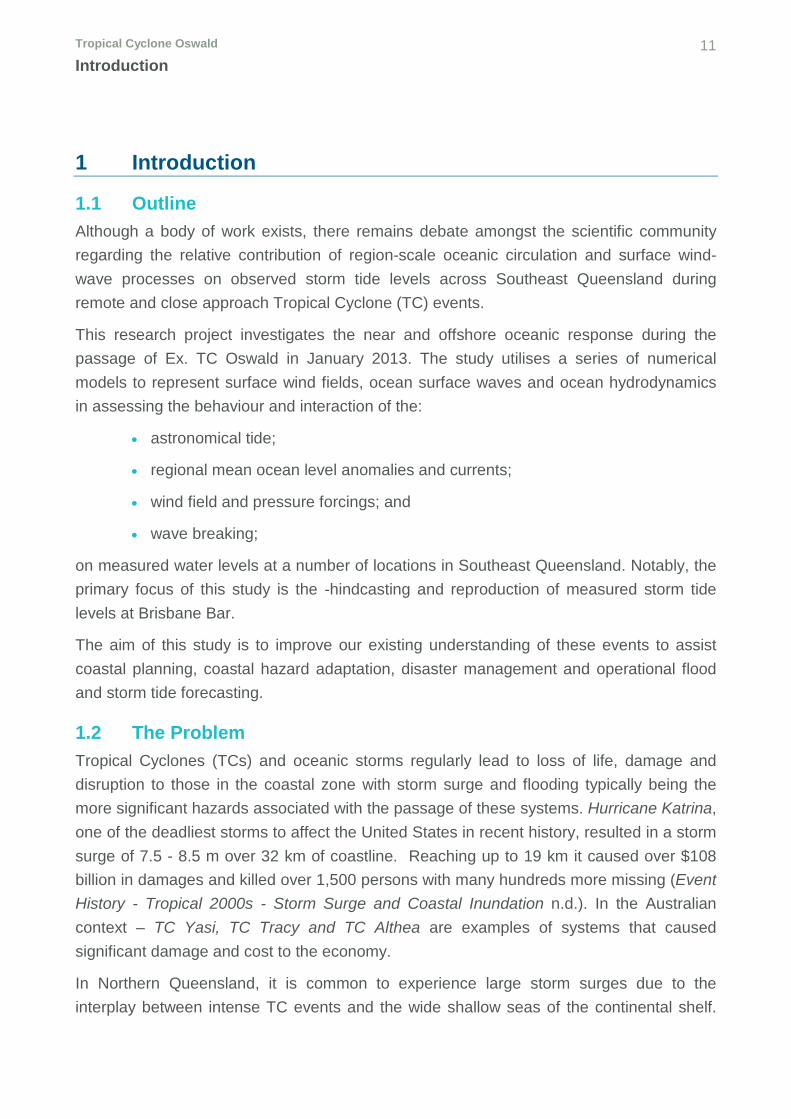
1.1 Outline Although a body of work exists, there remains debate amongst the scientific community regarding the relative contribution of region-scale oceanic circulation and surface wind-wave processes on observed storm tide levels across Southeast Queensland during remote and close approach Tropical Cyclone (TC) events.
This research project investigates the near and offshore oceanic response during the passage of Ex. TC Oswald in January 2013. The study utilises a series of numerical models to represent surface wind fields, ocean surface waves and ocean hydrodynamics in assessing the behaviour and interaction of the:
• astronomical tide;
• regional mean ocean level anomalies and currents;
• wind field and pressure forcings; and
• wave breaking;
on measured water levels at a number of locations in Southeast Queensland. Notably, the primary focus of this study is the -hindcasting and reproduction of measured storm tide levels at Brisbane Bar.
The aim of this study is to improve our existing understanding of these events to assist coastal planning, coastal hazard adaptation, disaster management and operational flood and storm tide forecasting.
1.2 The Problem Tropical Cyclones (TCs) and oceanic storms regularly lead to loss of life, damage and disruption to those in the coastal zone with storm surge and flooding typically being the more significant hazards associated with the passage of these systems. Hurricane Katrina, one of the deadliest storms to affect the United States in recent history, resulted in a storm surge of 7.5 - 8.5 m over 32 km of coastline. Reaching up to 19 km it caused over $108 billion in damages and killed over 1,500 persons with many hundreds more missing (Event History - Tropical 2000s - Storm Surge and Coastal Inundation n.d.). In the Australian context – TC Yasi, TC Tracy and TC Althea are examples of systems that caused significant damage and cost to the economy.
In Northern Queensland, it is common to experience large storm surges due to the interplay between intense TC events and the wide shallow seas of the continental shelf.
Tropical Cyclone Oswald 12 Introduction
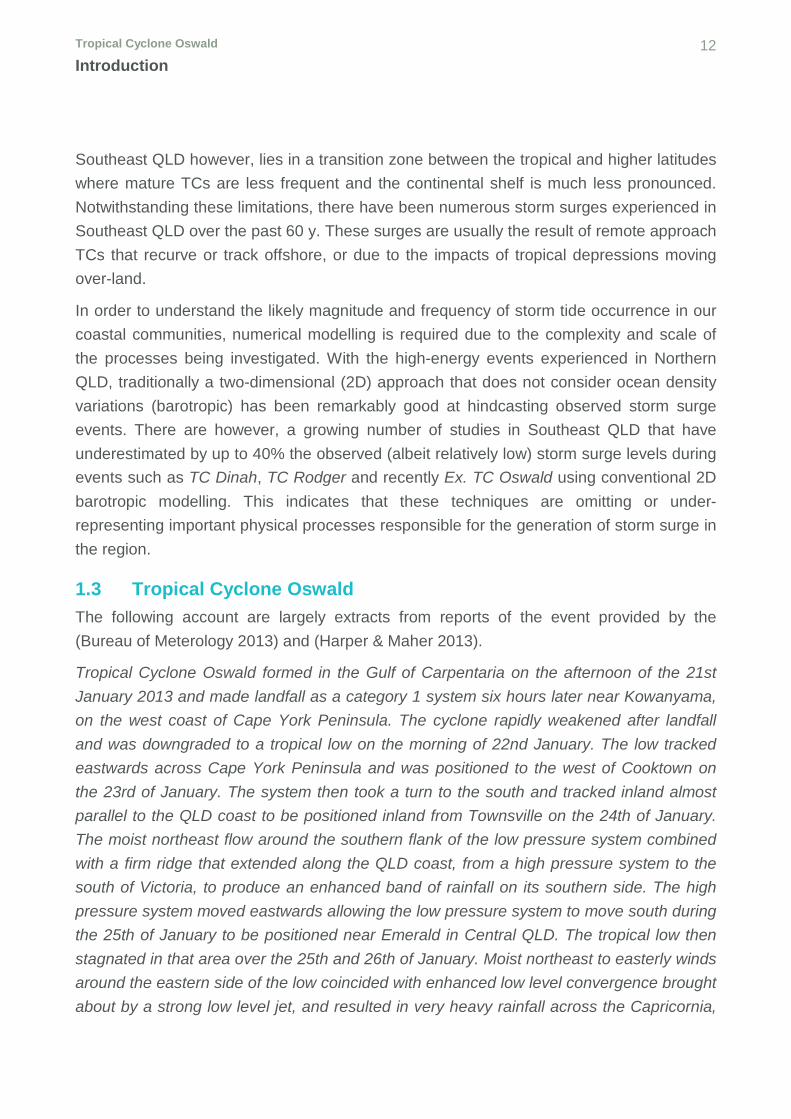
Southeast QLD however, lies in a transition zone between the tropical and higher latitudes where mature TCs are less frequent and the continental shelf is much less pronounced. Notwithstanding these limitations, there have been numerous storm surges experienced in Southeast QLD over the past 60 y. These surges are usually the result of remote approach TCs that recurve or track offshore, or due to the impacts of tropical depressions moving over-land.
In order to understand the likely magnitude and frequency of storm tide occurrence in our coastal communities, numerical modelling is required due to the complexity and scale of the processes being investigated. With the high-energy events experienced in Northern QLD, traditionally a two-dimensional (2D) approach that does not consider ocean density variations (barotropic) has been remarkably good at hindcasting observed storm surge events. There are however, a growing number of studies in Southeast QLD that have underestimated by up to 40% the observed (albeit relatively low) storm surge levels during events such as TC Dinah, TC Rodger and recently Ex. TC Oswald using conventional 2D barotropic modelling. This indicates that these techniques are omitting or under-representing important physical processes responsible for the generation of storm surge in the region.
1.3 Tropical Cyclone Oswald The following account are largely extracts from reports of the event provided by the (Bureau of Meterology 2013) and (Harper & Maher 2013).
Tropical Cyclone Oswald formed in the Gulf of Carpentaria on the afternoon of the 21st January 2013 and made landfall as a category 1 system six hours later near Kowanyama, on the west coast of Cape York Peninsula. The cyclone rapidly weakened after landfall and was downgraded to a tropical low on the morning of 22nd January. The low tracked eastwards across Cape York Peninsula and was positioned to the west of Cooktown on the 23rd of January. The system then took a turn to the south and tracked inland almost parallel to the QLD coast to be positioned inland from Townsville on the 24th of January. The moist northeast flow around the southern flank of the low pressure system combined with a firm ridge that extended along the QLD coast, from a high pressure system to the south of Victoria, to produce an enhanced band of rainfall on its southern side. The high pressure system moved eastwards allowing the low pressure system to move south during the 25th of January to be positioned near Emerald in Central QLD. The tropical low then stagnated in that area over the 25th and 26th of January. Moist northeast to easterly winds around the eastern side of the low coincided with enhanced low level convergence brought about by a strong low level jet, and resulted in very heavy rainfall across the Capricornia,
Tropical Cyclone Oswald 13 Introduction
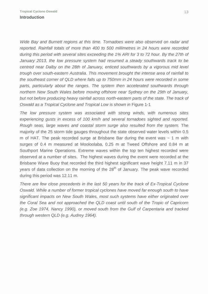
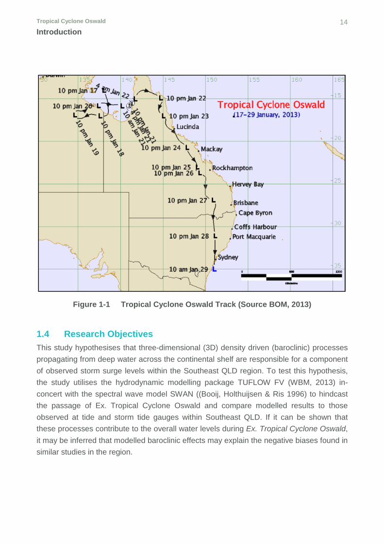
Wide Bay and Burnett regions at this time. Tornadoes were also observed on radar and reported. Rainfall totals of more than 400 to 500 millimetres in 24 hours were recorded during this period with several sites exceeding the 1% ARI for 3 to 72 hour. By the 27th of January 2013, the low pressure system had resumed a steady southwards track to be centred near Dalby on the 28th of January, enticed southwards by a vigorous mid level trough over south-eastern Australia. This movement brought the intense area of rainfall to the southeast corner of QLD where falls up to 750mm in 24 hours were recorded in some parts, particularly about the ranges. The system then accelerated southwards through northern New South Wales before moving offshore near Sydney on the 29th of January, but not before producing heavy rainfall across north-eastern parts of the state. The track of Oswald as a Tropical Cyclone and Tropical Low is shown in Figure 1-1
The low pressure system was associated with strong winds, with numerous sites experiencing gusts in excess of 100 km/h and several tornadoes sighted and reported. Rough seas, large waves and coastal storm surge also resulted from the system. The majority of the 25 storm tide gauges throughout the state observed water levels within 0.5 m of HAT. The peak recorded surge at Brisbane Bar during the event was ~ 1 m with surges of 0.4 m measured at Mooloolaba, 0.25 m at Tweed Offshore and 0.84 m at Southport Marine Operations. Extreme waves within the top ten highest recorded were observed at a number of sites. The highest waves during the event were recorded at the Brisbane Wave Buoy that recorded the third highest significant wave height 7.11 m in 37 years of data collection on the morning of the 28th of January. The peak wave recorded during this period was 12.11 m.
There are few close precedents in the last 50 years for the track of Ex-Tropical Cyclone Oswald. While a number of former tropical cyclones have moved far enough south to have significant impacts on New South Wales, most such systems have either originated over the Coral Sea and not approached the QLD coast until south of the Tropic of Capricorn (e.g. Zoe 1974, Nancy 1990), or moved south from the Gulf of Carpentaria and tracked through western QLD (e.g. Audrey 1964).
1.4 Research Objectives This study hypothesises that three-dimensional (3D) density driven (baroclinic) processes propagating from deep water across the continental shelf are responsible for a component of observed storm surge levels within the Southeast QLD region. To test this hypothesis, the study utilises the hydrodynamic modelling package TUFLOW FV (WBM, 2013) in-concert with the spectral wave model SWAN ((Booij, Holthuijsen & Ris 1996) to hindcast the passage of Ex. Tropical Cyclone Oswald and compare modelled results to those observed at tide and storm tide gauges within Southeast QLD. If it can be shown that these processes contribute to the overall water levels during Ex. Tropical Cyclone Oswald, it may be inferred that modelled baroclinic effects may explain the negative biases found in similar studies in the region.
Tropical Cyclone Oswald 15 Introduction
The specific objectives are:
• Collate available meteorological, oceanographic and topographic data required to setup a series of model experiments;
• Ensure that the available meteorological datasets are representative of observed conditions during Ex. TC. Oswald;
• Develop and test the hydrodynamic model TUFLOW FV. Prepare a model domain and set of parameters that are suitable for storm tide assessment;
• Develop and test a series of spectral wave models using SWAN. Prepare a model domain and set of parameters that are suitable for storm tide assessment;
• Calibrate the TUFLOW FV model to accurately represent the astronomical tides for the month of January 2013;
• Calibrate the SWAN model to accurately represent wave conditions for the month of January 2013;
• Complete a series of two-dimensional, depth-averaged hindcasts of Ex. TC Oswald, by varying the input forcing’s: astronomical tide, meteorological and wave input;
• Complete a series of three-dimensional, depth-averaged hindcasts of Ex. TC Oswald, by varying the input forcing’s: astronomical tide, meteorological and wave input;
• Undertake sensitivity testing on the effects of model resolution;
• Identify scope for further research.
1.5 Report Summary Key items investigated and undertaken for this study include:
• Literature Review: Review of applicable physical processes, relevant local and international studies (refer Chapter 2).
• Study Methodology (refer Chapter 3).
• Data Collation and Analysis: An analysis and overview of the comprehensive data collation process completed (refer Chapter 4).
• Model Setup: Configuration and details of the TUFLOW FV hydrodynamic and SWAN spectral wave model (refer Chapter 5);
Tropical Cyclone Oswald 16 Introduction
• Model Calibration: The astronomical tide and wave calibration process and results (refer Chapter 6)
• Experimental Hindcast Runs: Design and rationale of each experimental run conducted (refer Chapter 7).
• Results and Discussion: Presentation and discussion of the model Experimental Hindcast Runs (refer Chapters 8 and 9).
Tropical Cyclone Oswald 17 Literature Review
2 Literature Review
This section provides an overview of three main areas:
• The physical processes involved in the generation of coastal storm surge;
• Review of recent storm tide studies within the Southeast QLD region; and
• Investigation of relevant studies in the area of tropical cyclone and three dimensional ocean modelling.
2.1 Physical Processes
2.1.1 Introduction The passage of synoptic-scale meteorological systems such as Tropical Cyclones, Extra-Tropical Systems and East Coast Lows bring with them heavy rainfall, destructive winds and affect the ocean on a range of spatial scales (Harper et al. 2001). From a coastal management perspective, coastal inundation and erosion associated with the storm surge and extreme waves generated by these events are of primary concern.
The following sections provide an overview of the main dynamic and static physical processes that contribute to the generation and propagation of storm tide hazard within the Queensland (QLD) region including:
• Synoptic scale oceanic storm systems;
• Ocean bathymetry, coastal morphology and topography;
• The astronomical tide;
• Ocean density structure, internal waves, coastal currents and seasonal ocean setup; and
• Offshore and near-shore surface wave processes including wave shoaling, wave setup, run-up and overland wave propagation.
Each of the aforementioned factors contribute in a non-uniform manner to observed water levels measured during coastal storm events. Importantly, these factors act to influence each other in a complex non-linear fashion over the large temporal and spatial scales they act upon.
Tropical Cyclone Oswald 18 Literature Review
2.1.2 Overview of Storm Tide Components Figure 2-1 provides an overview of the major storm tide components.
• Astronomical tide plays an important role in determining the depth of water to generate surge or wave attack during a storm.
• Wind driven surge: Transfer of momentum from wind shear stress is imparted to the water column. The leads to the generation of currents and in regions adjacent to the coastline, water can ‘heap’ up against the coast. The shallower the water, the higher surge that can occur.
• Pressure surge: This is also known as the so-called inverse-barometer effect that results in about 1cm rise for every hPa mean sea level pressure drop. Usually not as significant as the wind driven surge.
• Extreme winds acting on the ocean surface generate wind waves. As these wave propagate into shallow water they begin to shoal and break. Some of the kinetic and potential energy associated with wave forms an onshore current component. This onshore component of breaking wave energy results in a increased mean water level at the beach face known as wave setup (Longuet-Higgins & Stewart 1964).
• The storm tide is the combination of the astronomical tide, wind and pressure surge and wave setup.
• In addition to storm tide, residual energy from the runup of individual waves and surf beat can result in intermittent water levels above the wave setup level due to wave action. These waves can propagate inland causing significant damage to coastal structures and infrastructure.
Storm tide is often measured using the tidal residual, or the difference between the measured water level and the predicted tide as follows:
Figure 2-1 provides a schematic of each storm tide component. The term SWL refers to the so-called ‘still water level’ and represents the level that the storm surge would reach without surface gravity wave processes. The mean water level (MWL) is the elevated water levels experienced adjacent to the beach due to wave setup, which acts on top of the SWL. The storm tide can be measured above the Australian Height Datum (AHD) or at times the Lowest Astronomical Tide datum and this is often a cause of confusion. The term HAT stands for the Highest Astronomical Tide and represents the maximum height at which the astronomical tide can reach at a given location due to just
Tropical Cyclone Oswald 19 Literature Review
gravitation forces alone, however due to the effects of weather it is regular exceeded. HAT is an important level as generally dwellings and public infrastructure are constructed above it and therefore storm tide exceeding HAT can have disastrous effects on the community.
Figure 2-1 Storm Tide Components. Reproduced with permission (Harper et al. 2001)
2.1.3 Equations of Motion The physical response of the ocean to external and internal forces can be simplified and modelled through the usage of the so-called Non-Linear Shallow Water Long Wave equations. These equations are derived from the viscous Reynolds equations (Harper et al. 2001) assuming hydrostatic and Boussinesq approximations as follows:
• Hydrostatic approximation: This assumes that the horizontal scale is large compared to the vertical scale and that the vertical pressure gradient is a product of the density and gravitation acceleration (buoyancy)(Hydrostatic balance - AMS Glossary n.d.) .
• Boussinesq approximation: Assumes that density differences (in a given layer) are small enough to be neglected and that density differences only affect the acceleration due to gravity (buoyancy term).
• The fluid is incompressible, vertical accelerations can be ignored and density variation affect the buoyancy of the fluid only
Tropical Cyclone Oswald 20 Literature Review
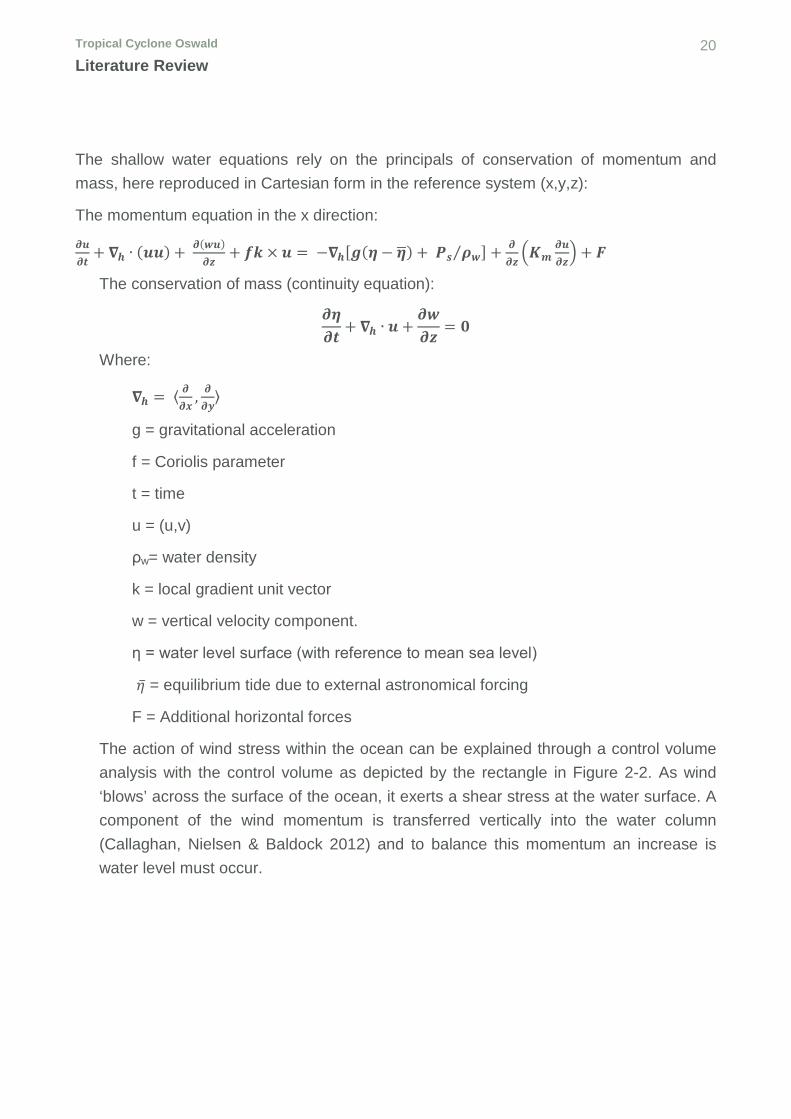
The shallow water equations rely on the principals of conservation of momentum and mass, here reproduced in Cartesian form in the reference system (x,y,z):
η = water level surface (with reference to mean sea level)
�̅�𝜂 = equilibrium tide due to external astronomical forcing
F = Additional horizontal forces
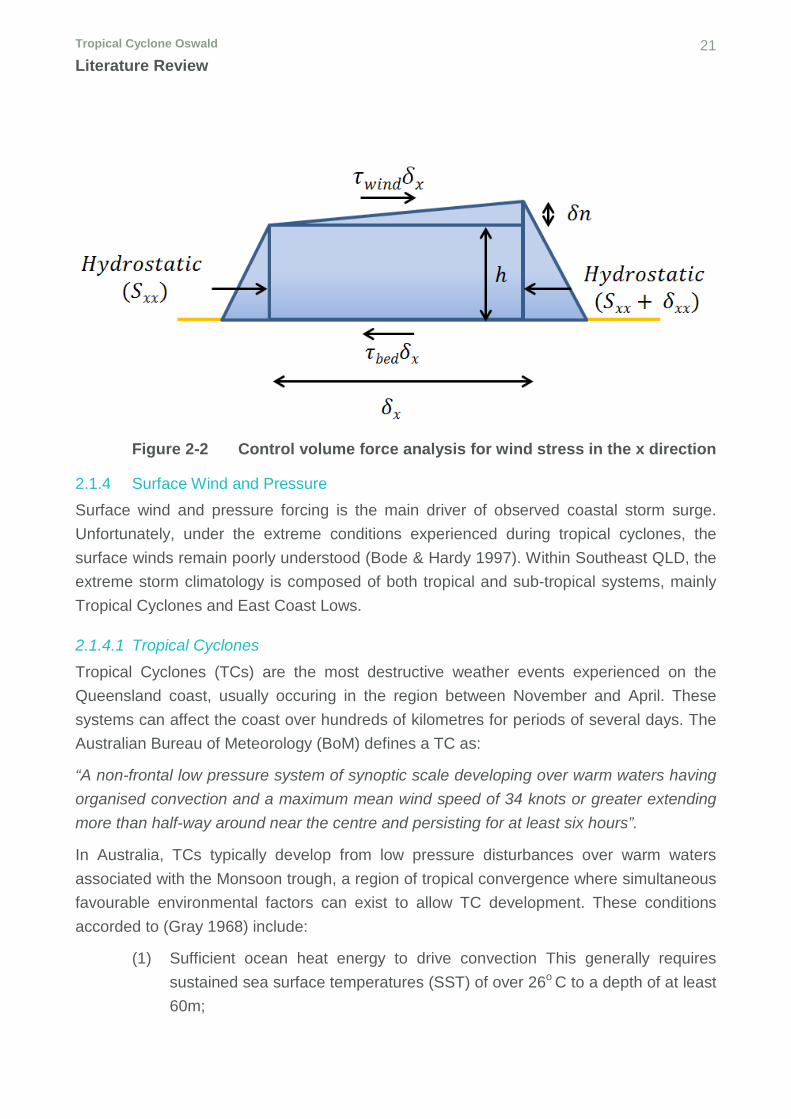
The action of wind stress within the ocean can be explained through a control volume analysis with the control volume as depicted by the rectangle in Figure 2-2. As wind ‘blows’ across the surface of the ocean, it exerts a shear stress at the water surface. A component of the wind momentum is transferred vertically into the water column (Callaghan, Nielsen & Baldock 2012) and to balance this momentum an increase is water level must occur.
Tropical Cyclone Oswald 21 Literature Review
Figure 2-2 Control volume force analysis for wind stress in the x direction
2.1.4 Surface Wind and Pressure Surface wind and pressure forcing is the main driver of observed coastal storm surge. Unfortunately, under the extreme conditions experienced during tropical cyclones, the surface winds remain poorly understood (Bode & Hardy 1997). Within Southeast QLD, the extreme storm climatology is composed of both tropical and sub-tropical systems, mainly Tropical Cyclones and East Coast Lows.
2.1.4.1 Tropical Cyclones
Tropical Cyclones (TCs) are the most destructive weather events experienced on the Queensland coast, usually occuring in the region between November and April. These systems can affect the coast over hundreds of kilometres for periods of several days. The Australian Bureau of Meteorology (BoM) defines a TC as:
“A non-frontal low pressure system of synoptic scale developing over warm waters having organised convection and a maximum mean wind speed of 34 knots or greater extending more than half-way around near the centre and persisting for at least six hours”.
In Australia, TCs typically develop from low pressure disturbances over warm waters associated with the Monsoon trough, a region of tropical convergence where simultaneous favourable environmental factors can exist to allow TC development. These conditions accorded to (Gray 1968) include:
(1) Sufficient ocean heat energy to drive convection This generally requires sustained sea surface temperatures (SST) of over 26o C to a depth of at least 60m;
Tropical Cyclone Oswald 22 Literature Review
(2) Enhanced humidity through the mid-troposphere and conditional instability;
(5) Formation needs to be far enough from the equator to allow sufficient Coriolis deflection and rotation (typically greater than 5 degrees of latitude although there have been exceptions).
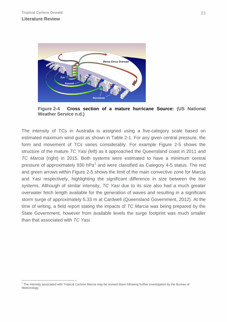
A mature TC is characterised by largely symmetrical ‘core’ with winds rotating clockwise (anti-clockwise) in the southern (northern) hemisphere around an inner ‘eye’ which is typically 30-50 km in diameter (Harper et al. 2001). This eye region is associated with the lowest atmospheric pressure and is relatively calm compared to the violent and destructive winds within the convective cumulonimbus clouds of the ‘eye-wall’ that surround the eye (refer to the purple and red colouration in the left panel of Figure 2-3 and as shown in Figure 2-4). For TCs approaching the QLD east coast from offshore, the maximum wind speeds are usually experienced to the south of the system where both the forward speed component of the moving storm and the wind direction act together. Outside of the eye-wall a series of convergent spiral rainbands can trail out for many hundreds of kilometres.
Figure 2-3 Mature Tropical Cyclone symmetrical form (left) and hybrid system (right) Source: (Bureau of Meterology n.d.))
Tropical Cyclone Oswald 23 Literature Review
Figure 2-4 Cross section of a mature hurricane Source: (US National Weather Service n.d.)
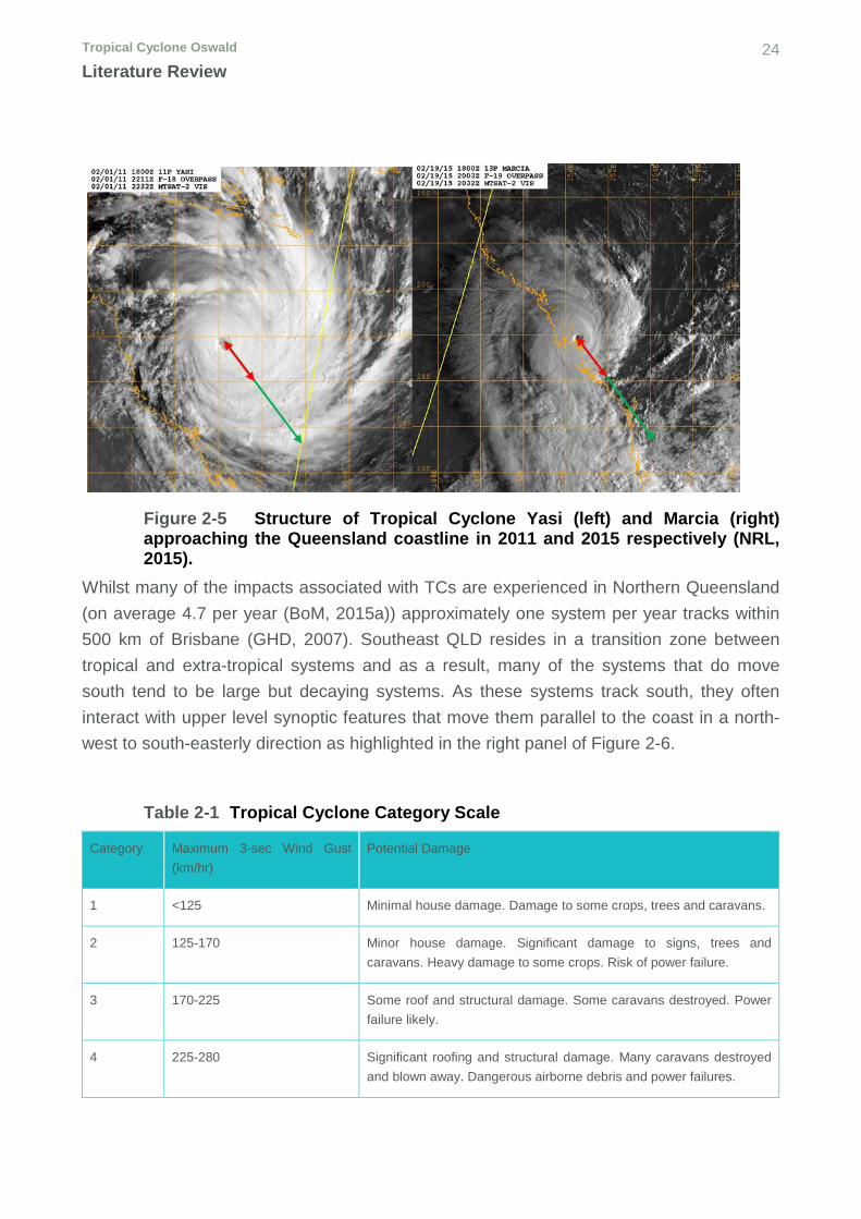
The intensity of TCs in Australia is assigned using a five-category scale based on estimated maximum wind gust as shown in Table 2-1. For any given central pressure, the form and movement of TCs varies considerably. For example Figure 2-5 shows the structure of the mature TC Yasi (left) as it approached the Queensland coast in 2011 and TC Marcia (right) in 2015. Both systems were estimated to have a minimum central pressure of approximately 930 hPa1 and were classified as Category 4-5 status. The red and green arrows within Figure 2-5 shows the limit of the main convective zone for Marcia and Yasi respectively, highlighting the significant difference in size between the two systems. Although of similar intensity, TC Yasi due to its size also had a much greater overwater fetch length available for the generation of waves and resulting in a significant storm surge of approximately 5.33 m at Cardwell (Queensland Government, 2012). At the time of writing, a field report stating the impacts of TC Marcia was being prepared by the State Government, however from available levels the surge footprint was much smaller than that associated with TC Yasi.
1 The intensity associated with Tropical Cyclone Marcia may be revised down following further investigation by the Bureau of Meteorology.
Tropical Cyclone Oswald 24 Literature Review
Figure 2-5 Structure of Tropical Cyclone Yasi (left) and Marcia (right) approaching the Queensland coastline in 2011 and 2015 respectively (NRL, 2015).
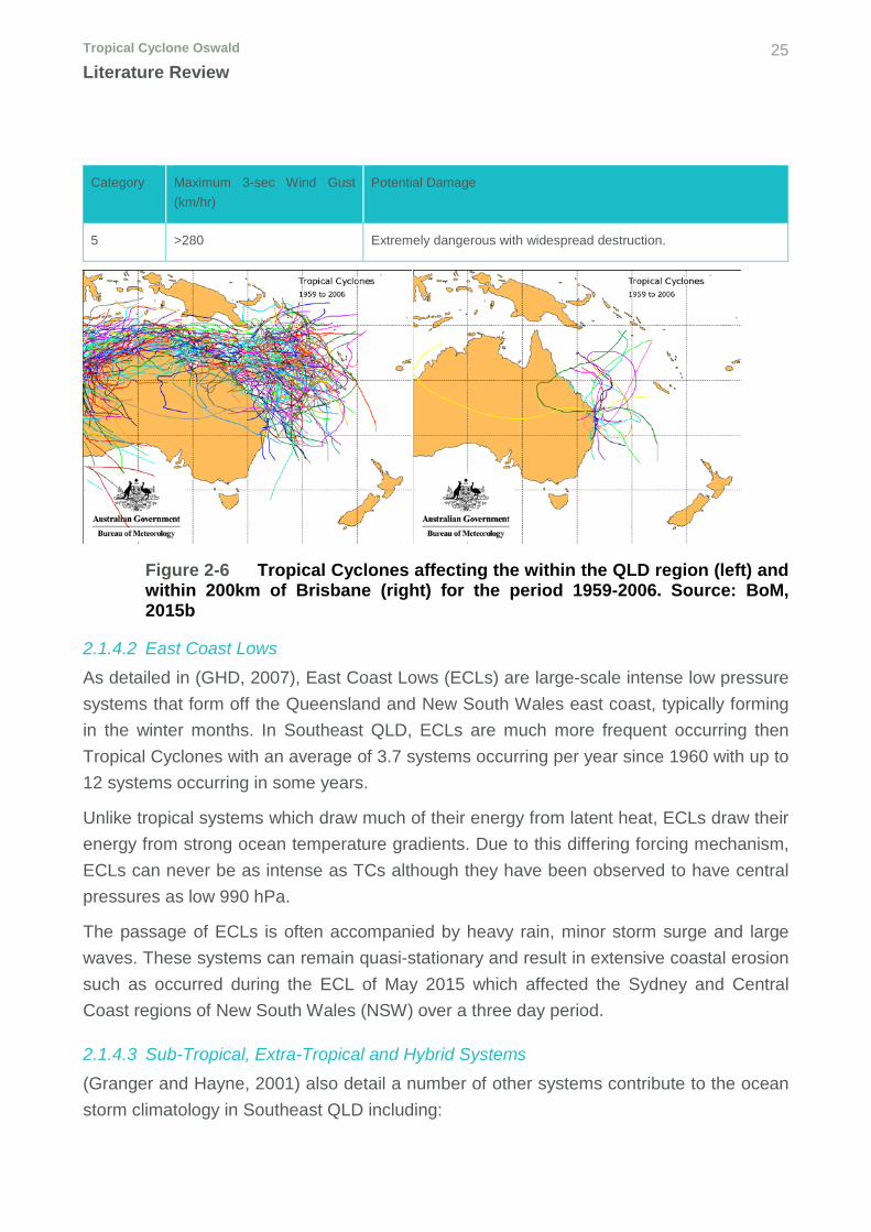
Whilst many of the impacts associated with TCs are experienced in Northern Queensland (on average 4.7 per year (BoM, 2015a)) approximately one system per year tracks within 500 km of Brisbane (GHD, 2007). Southeast QLD resides in a transition zone between tropical and extra-tropical systems and as a result, many of the systems that do move south tend to be large but decaying systems. As these systems track south, they often interact with upper level synoptic features that move them parallel to the coast in a north-west to south-easterly direction as highlighted in the right panel of Figure 2-6.
Table 2-1 Tropical Cyclone Category Scale
Category Maximum 3-sec Wind Gust (km/hr)
Potential Damage
1 <125 Minimal house damage. Damage to some crops, trees and caravans.
2 125-170 Minor house damage. Significant damage to signs, trees and caravans. Heavy damage to some crops. Risk of power failure.
3 170-225 Some roof and structural damage. Some caravans destroyed. Power failure likely.
4 225-280 Significant roofing and structural damage. Many caravans destroyed and blown away. Dangerous airborne debris and power failures.
Tropical Cyclone Oswald 25 Literature Review
Category Maximum 3-sec Wind Gust (km/hr)
Potential Damage
5 >280 Extremely dangerous with widespread destruction.
Figure 2-6 Tropical Cyclones affecting the within the QLD region (left) and within 200km of Brisbane (right) for the period 1959-2006. Source: BoM, 2015b
2.1.4.2 East Coast Lows
As detailed in (GHD, 2007), East Coast Lows (ECLs) are large-scale intense low pressure systems that form off the Queensland and New South Wales east coast, typically forming in the winter months. In Southeast QLD, ECLs are much more frequent occurring then Tropical Cyclones with an average of 3.7 systems occurring per year since 1960 with up to 12 systems occurring in some years.
Unlike tropical systems which draw much of their energy from latent heat, ECLs draw their energy from strong ocean temperature gradients. Due to this differing forcing mechanism, ECLs can never be as intense as TCs although they have been observed to have central pressures as low 990 hPa.
The passage of ECLs is often accompanied by heavy rain, minor storm surge and large waves. These systems can remain quasi-stationary and result in extensive coastal erosion such as occurred during the ECL of May 2015 which affected the Sydney and Central Coast regions of New South Wales (NSW) over a three day period.
2.1.4.3 Sub-Tropical, Extra-Tropical and Hybrid Systems
(Granger and Hayne, 2001) also detail a number of other systems contribute to the ocean storm climatology in Southeast QLD including:
Tropical Cyclone Oswald 26 Literature Review
• Sub-Tropical Cyclones: Intense low-pressure systems that don’t quite make it to TC intensity. They do not have the extreme eye wall winds required to be classed as TCs however due to large fetch lengths, they can still lead to large wave and surge events. Such systems can transform into extra-tropical systems or east coast lows.
• Decaying or south moving Tropical Cyclones can often interact with the passage of trough systems resulting in or extra-tropical transition or the so-called ‘weather bombs’. Rather than decaying as a tropical system, the gain further energy through interaction with other systems. This can result in rapid intensification.
• Finally, a storm can be in the form of a ‘hybrid’ system with structure similar to that provided in the right panel of Figure 2-3. These systems can be hard to classify and much of the convection can be to the south of the system.
TC Oswald was an unusual system to classify in that after making landfall as a ‘true’ Category 1 TC in the Gulf of Carpentaria, Ex-TC Oswald passed almost entirely overland through QLD and NSW as an intense inland low, affecting almost the entire east coast of Australia.
2.1.5 Astronomical Tide The astronomical tides are primarily the result of the gravitation forces of the moon and sun upon the earth; and the centrifugal forces produced by the earth and moon and earth and sun around their common centre of gravity (NOAA, 2013).
Normal to the earth’s surface, the gravity component of the earth is approximately nine million times stronger than that exerted by the moon. Thus the moon does not pull vertically, but tides propagate horizontally and act to ‘pile up’ water due to the horizontal component of the gravitation force, known as the Tractive Force. This results in a series of gravitationally driven sine waves that continuously sweep around the earth following the position of the moon (and sun).
Land masses act as a barrier to tidal wave propagation. Topography can also create local effects or restrain the tide acting to significantly change the speed of propagation. As the depth of the water shallows, the speed of forward movement of a traveling tidal wave is modified due to frictional forces of the bed and ocean current that act to slow the advance of tide.
The astronomical tide component of observed water levels can be represented as a linear combination of sine waves known as tidal constituents. These components can be extracted from a measured time history of sufficient length to extract tidal phase, amplitude
Tropical Cyclone Oswald 27 Literature Review
and frequency for each of the main 37 different tidal constituents using Fourier Analysis (Pawlowicz, Beardsley & Lentz 2002). The eight major diurnal and semi-diurnal constituents for Brisbane Bar and the tidal planes are provided in Table 2-2 and Table 2-3 respectively (Department of Transport and Main Roads 2014)
Table 2-2 Brisbane Bar Tidal Constituents
Constant Definition Amplitude (m) Phase (o) M2 Principal lunar semidiurnal
constituent 0.707 275.0
S2 Principal solar semidiurnal constituent
0.193 302.2
N2 Larger lunar elliptic semidiurnal constituent
0.138 265.3
K2 Lunisolar semidiurnal constituent 0.058 294.2
K1 Lunar diurnal constituent 0.212 171.1
O1 Lunar diurnal constituent 0.117 131.4
P1 Solar diurnal constituent 0.060 169.0
Q1 Larger lunar elliptic diurnal constituent
0.024 103.0
Whether a given region has diurnal (one high tide per day) or semi-diurnal (two high tide per day) can be classified based on the tidal ‘Form Factor’, a relationship between the major diurnal and semi diurnal constants. When F is less than or equal 0.5 the tide is semi-diurnal, if greater than 0.5 the tide is primarily diurnal (PCTMSL 2014). As shown in the equation below this indicates that Brisbane Bar and the Moreton Bay region can be classified as a semi-diurnal tide.
𝐹𝐹 =𝐾𝐾1 + 𝑂𝑂1
𝑀𝑀2 + 𝑆𝑆2=
0.212 + 0.1170.707 + 0.193
= 0.37
Where the tidal constants are previously described in Table 2-2 Table 2-3 2015 Brisbane Bar Tidal Planes
Constant Level (mLAT) Level (mAHD) Mean Sea Level 1.27 0.03
Australian Height Datum 1.243 0.00
Mean High Water Neaps 1.78 0.54
Mean High Water Springs 2.17 0.93
Highest Astronomical Tide 2.73 1.49
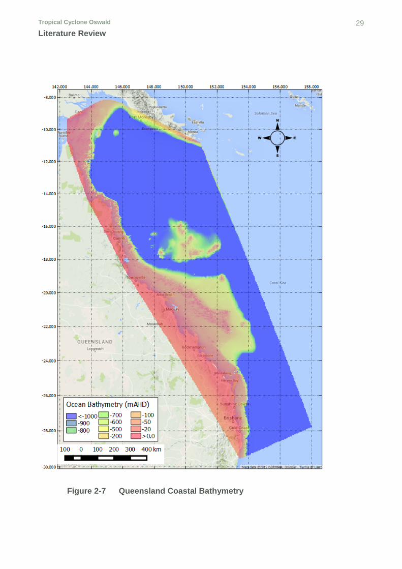
2.1.6 Bathymetry and Coastal Morphology The underlying ocean bathymetry and coastal morphology determine the propagation of the astronomical tides and storm surges from deep water into coastal near-shore regions. The bathymetry of the QLD Coast south from Townsville is characterised by a large continental shelf extending up to 200 km offshore reducing sharply east of Bundaberg and then tapering to approximately 40 km at the QLD/NSW border (refer Figure 2-7). The presence of the continental shelf in northern QLD has allowed the formation of the Great Barrier Reef that acts as an important barrier in the dissipation of offshore wave energy, reducing the threat of wave attack during extreme events. Although reducing wave attack, the shallow water region of the Great Barrier Reef Lagoon at its widest enhances the threat of extreme storm surge to our Northern Coastal communities.
The exposed coastline of the Gold Coast, the Sunshine Coast and the barrier islands of Stradbroke, Moreton, Bribie and Fraser Islands are all subject to high-energy wave attack and this has resulted in the iconic beaches that we observe on these stretches of coast. While Moreton Bay is largely sheltered by extreme wave effects by the Barrier Islands, the region represents a relatively shallow coastal embayment with much of the bathymetry between 0 to 10 m below Mean Sea Level (MSL). Due to its shallow nature it is more vulnerable to storm surge than the aforementioned beach regions.
Major river systems that empty into Moreton Bay include the Caboolture, Pine, Brisbane, Logan and Albert Rivers that in flood can introduce a significant amount of freshwater and sediment.
Tropical Cyclone Oswald 29 Literature Review
Figure 2-7 Queensland Coastal Bathymetry
Tropical Cyclone Oswald 30 Literature Review
2.1.7 Storm Surge Storm surges are a result of meteorological forcing on the ocean surface. They manifest as surface long waves that can cause persistent increased water levels to those usually associated with the astronomical tide (Harper et al., 2001). During extreme wind events such as TCs, ECLs and Extra-Tropical Systems, the magnitude of the surge is primarily forced by surface wind shear stress with atmospheric pressure forming a lesser component of the overall surge.
As a storm system approaches the coast, the storm surge at a given location is influenced by a complex combination of factors such as:
• The approach speed, intensity, direction and size of the storm;
• The phase of the astronomical tide during the passage of the system;
• The shape and scale of the coastal bathymetry and morphology. i.e. the presence and slope of the continental shelf, shallow coastal embayment’s, beaches, coastal lowlands, offshore reefs, barrier islands and riverine systems; and
• The role of surface gravity (wind driven) waves and interaction between the atmosphere and ocean at the air-sea interface.
2.1.8 Surface Wind Waves In deep water, surface wind waves play an important role in the mixing of the upper ocean through turbulence and oscillatory motion. In shallow regions, wave shoaling can act to impart energy into the water column resulting in wave induced currents and the wave setup component of storm tide.
Wind waves and swell are essentially a form of gravity wave generated through the shearing effects of the wind on the ocean surface. As the wind begins to blow it produces random pressure fluctuations that build very small waves (Stewart 2008). As the wind continues to blow these small waves grow in size which creates larger pressure differences and the waves grow rapidly. As these waves grow they begin to interact producing waves of longer wavelengths (Hasselmann et al. 1973) that propagate away from the generation site. For a given wind speed, duration, fetch and water depth wave heights will continue to grow until the reach a state of equilibrium known as a ‘fully arisen sea’.
By nature waves are inherently non-linear (Stewart 2008) however we can approximate real wave behaviour through linear wave theory. This leads to fundamental expressions for
Tropical Cyclone Oswald 31 Literature Review
wave height, wave period, frequency, number, celerity, dispersion, phase and group velocity and wave energy which are not repeated here.
In reality, the waves we observe at the beach are a complex combination of semi-random energy waves that advect energy across surface and through the upper ocean, each with their own frequency, direction and source. There is still on-going research into the propagation of waves however which with some simplifications, can be assessed using the concept of a wave spectrum (Stewart 2008). This study will use a so-called third generation wave model (SWAN) to model the evolution and decay of the directional wave spectrum F(ƒ,θ) where ƒ is frequency and θ is the direction of propagation ((Harper et al. 2001).
Waves transfer momentum to the water column through an excess pressure force and horizontal momentum flux known as wave radiation stress (Longuet-Higgings and Stewart 1964). Radiation stresses can occur in both deep and shallow waters however for the purposes of storm tide assessment and coastal morphological studies the action of waves for the latter can become significant. Waves start to be affected by bed friction when the depth is approximately half the wavelength, as the depth becomes shallower the waves increase in steepness, shoal and eventually break. The ensuing energy imparted by radiation stresses lead to wave induced currents, wave setup, surf beat and wave run-up.
Inside the surf zone radiation stresses decrease rapidly as you approach the shore due to the depth limited wave heights. The process of breaking wave setup is highlighted in Figure 2-8 whereby an elevated mean water level can be maintained through the surf zone according to the following relationship:
𝜕𝜕𝜂𝜂𝜕𝜕𝜕𝜕
=1𝜌𝜌𝜌𝜌ℎ
∙𝜕𝜕𝑆𝑆𝑥𝑥𝑥𝑥𝜕𝜕𝜕𝜕
+1𝜌𝜌𝜌𝜌ℎ
∙ (𝜏𝜏𝑤𝑤𝑤𝑤𝑤𝑤𝑤𝑤 − 𝜏𝜏𝑏𝑏𝑏𝑏𝑤𝑤)
Where:
�̅�𝜂 = Level above mean sea level (m)
𝜌𝜌 = Water Density (kg/m3)
𝜌𝜌 = Gravitational acceleration (m/s2)
ℎ = Water depth (relative to mean water sea level (m)
𝑆𝑆𝑥𝑥𝑥𝑥 = Wave radiation stress (Pa)
𝜏𝜏 = (Pa)
Figure 2-8 Wave setup at the shoreline (after (Hanslow & Nielsen 1992)
Tropical Cyclone Oswald 32 Literature Review
2.1.9 Limitations in our current understanding of wave-surge physics The review of (Bode & Hardy 1997) made a number of observations with regard to the status of storm tide modelling and model physics which almost twenty years later remain areas of intense research focus. Two key points were in relation to the need to include surge-wave interactions. Importantly:
• The current method of specifying surface stress as a function of wind speed only, underestimates the role of surface waves. Waves are the roughness element and they move in both space and time and that the physics at the air interface is very complex and poorly understood, particually at extreme wind speeds;
• If the wind speed and direction is known, which is very unlikely most of the time, the surface drag coefficient is the single most important factor in determining the transfer of momentum to the water column.
So it is possible that limitations to our current implementation of these important physical processes is responsible for a component of the ‘missing’ storm tide levels observed within the region.
2.1.10 Ocean Vertical Structure The vertical state of the ocean establishes the kind of disturbances that can propagate through the internal ocean. As this study is looking at the potential for density driven effects along the continental shelf during the passage of extreme weather events, the three-dimensional state prior and the likely mixing during the event are explored.
Vertically, the ocean can be described by three main regions:
• The mixed boundary layer: The surface region of ocean subject to atmospheric forcing and the ocean currents driven by wind stress and pressure gradients. Salinity and temperature are close to constant in this layer (Stewart 2008);
• The thermocline: The region below the mixed layer where there is a rapid change in temperature and thus density; and
• The deep ocean: The region below the thermocline typically less than 1500 m below sea level.
Seawater density is a function of pressure, salinity and temperature that is calculated using the equation of state. In most oceanic situations, and in particular in the upper 1500 m of the ocean, the effect of the vertical salinity gradient on density is much smaller than the effect of the vertical temperature gradient (Tomczak & Godfrey 2003).
Tropical Cyclone Oswald 33 Literature Review
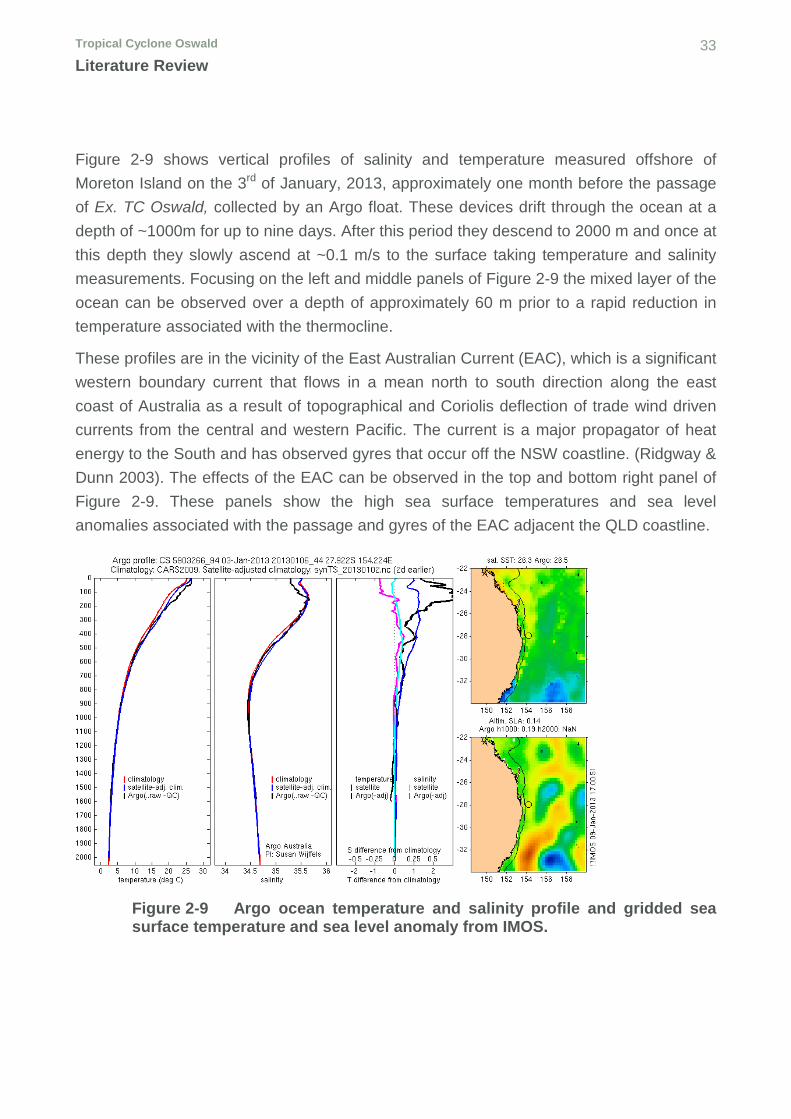
Figure 2-9 shows vertical profiles of salinity and temperature measured offshore of Moreton Island on the 3rd of January, 2013, approximately one month before the passage of Ex. TC Oswald, collected by an Argo float. These devices drift through the ocean at a depth of ~1000m for up to nine days. After this period they descend to 2000 m and once at this depth they slowly ascend at ~0.1 m/s to the surface taking temperature and salinity measurements. Focusing on the left and middle panels of Figure 2-9 the mixed layer of the ocean can be observed over a depth of approximately 60 m prior to a rapid reduction in temperature associated with the thermocline.
These profiles are in the vicinity of the East Australian Current (EAC), which is a significant western boundary current that flows in a mean north to south direction along the east coast of Australia as a result of topographical and Coriolis deflection of trade wind driven currents from the central and western Pacific. The current is a major propagator of heat energy to the South and has observed gyres that occur off the NSW coastline. (Ridgway & Dunn 2003). The effects of the EAC can be observed in the top and bottom right panel of Figure 2-9. These panels show the high sea surface temperatures and sea level anomalies associated with the passage and gyres of the EAC adjacent the QLD coastline.
Figure 2-9 Argo ocean temperature and salinity profile and gridded sea surface temperature and sea level anomaly from IMOS.
Tropical Cyclone Oswald 34 Literature Review
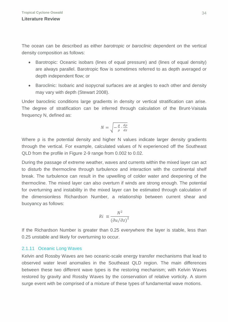
The ocean can be described as either barotropic or baroclinic dependent on the vertical density composition as follows:
• Barotropic: Oceanic isobars (lines of equal pressure) and (lines of equal density) are always parallel. Barotropic flow is sometimes referred to as depth averaged or depth independent flow; or
• Baroclinic: Isobaric and isopycnal surfaces are at angles to each other and density may vary with depth (Stewart 2008).
Under baroclinic conditions large gradients in density or vertical stratification can arise. The degree of stratification can be inferred through calculation of the Brunt-Vaisala frequency N, defined as:
𝑁𝑁 = �−𝑔𝑔𝜌𝜌∙ 𝑤𝑤𝜌𝜌𝑤𝑤𝑑𝑑
Where p is the potential density and higher N values indicate larger density gradients through the vertical. For example, calculated values of N experienced off the Southeast QLD from the profile in Figure 2-9 range from 0.002 to 0.02.
During the passage of extreme weather, waves and currents within the mixed layer can act to disturb the thermocline through turbulence and interaction with the continental shelf break. The turbulence can result in the upwelling of colder water and deepening of the thermocline. The mixed layer can also overturn if winds are strong enough. The potential for overturning and instability in the mixed layer can be estimated through calculation of the dimensionless Richardson Number, a relationship between current shear and buoyancy as follows:
𝑅𝑅𝑇𝑇 ≡𝑁𝑁2
(𝜕𝜕𝑅𝑅 𝜕𝜕𝜕𝜕)⁄ 2
If the Richardson Number is greater than 0.25 everywhere the layer is stable, less than 0.25 unstable and likely for overturning to occur.
2.1.11 Oceanic Long Waves Kelvin and Rossby Waves are two oceanic-scale energy transfer mechanisms that lead to observed water level anomalies in the Southeast QLD region. The main differences between these two different wave types is the restoring mechanism; with Kelvin Waves restored by gravity and Rossby Waves by the conservation of relative vorticity. A storm surge event with be comprised of a mixture of these types of fundamental wave motions.
Tropical Cyclone Oswald 35 Literature Review
2.1.11.1 Kelvin Waves
Coastal Kelvin Waves (or coastally trapped waves) can travel on the surface (Barotropic) or as internal waves (Baroclinic) and balance the Coriolis Force against a topographic boundary. In the Southern Hemisphere they always propagate with the coast on the left. Coastally trapped waves as a result of TCs have been investigated at length in the Australian region by the likes of (Tang & Grimshaw 1995), (Woodham et al. 2013), (Eliot & Pattiaratchi 2010) which have shown that waves move around the continent as continuous features with their amplitude modulated by the width of the continental shelf ( Waves travel faster with greater continental shelf width). The amplitude of a coastal Kelvin wave is at maximum at the coast and negligible at a distance defined by the Rossby Radius of deformation, which defines the distance over which Coriolis forces start to become as important as buoyancy and gravitation wave speed processes. In a Barotropic ocean the Rossby Radius of Deformation is defined by:
�𝜌𝜌𝑔𝑔𝑓𝑓
where g = gravitational acceleration;
H = water depth; and
f = 2Ω sin𝜙𝜙 or Coriolis Parameter (approx.. 0.66E-06 for the Brisbane region).
Table 2-4 provides a summary of calculated Rossby Radii of Deformation at different depths off the Southeast QLD coast and shows that there is a considerable distance that a current must travel prior to be deflected, particularly in deep water. Baroclinic waves can be deflected over relatively shorter lengths, due largely to the smaller difference in density between ocean layers. As defined in (Chelton et al. 1998), away from the tropics, i.e. less than ±5o latitude the baroclinic Rossby Radius of Deformation is computed from the baroclinic gravity-wave phase speed, c, and the Coriolis parameter, f, as follows:
𝑀𝑀 = 𝑐𝑐𝑓𝑓 Where: 𝑃𝑃 = �𝜌𝜌 ∆𝜌𝜌
𝜌𝜌𝐻𝐻1𝐻𝐻2𝐻𝐻1+𝐻𝐻2
Baroclinic wave celerity
where H1 and H2 represent the top and bottom of the ocean layer considered respectively.
Tropical Cyclone Oswald 36 Literature Review
Table 2-4 Barotropic and Baroclinic Rossby Radii of Deformation off Southeast QLD
Depth Barotropic Rossby Radius of Deformation (km)
Baroclinic Rossy Radius of Deformation (km)
50 140 30-50 km
100 320
250 650
500 910
1000 1290
2.1.11.2 Rossby Waves
Rossby Waves form due to the requirements to conserve potential vorticity. In a Barotropic ocean as water is pushed eastward over a reducing depth, to conserve potential vorticity the relative vorticity must increase. In the Southern Hemisphere, as depth decreases there is an anticlockwise rotation of the water column. Equally as water flows equator-ward under constant depth the Coriolis parameter decreases to there must be a increase in vorticity leading to anti-clockwise flow.
Π =ƒ𝜌𝜌∙𝜕𝜕𝜌𝜌𝜕𝜕𝜕𝜕
=𝜉𝜉 + ƒ𝑔𝑔
Where f is the Coriolis Parameter
p is the water density
H is the total water depth
z is the water depth
𝜉𝜉 is the relative vorticity
2.1.12 Internal Waves Internal waves propagate within the interior of the ocean, typically within the thermocline at the interface of differing density layers (refer Figure 2-10). They can be thought of as similar to surface gravity waves (Thorpe 1999). As stated in (Dukhovskoy, Morey & O’Brien 2009), internal wave frequencies can range from an upper limit of the Brunt-Vaisala frequency to a minimum of the Coriolis frequency, however they generally span from a few tens of cycles per hour to one cycle per Coriolis period. The internal response of the ocean over a shelf to a cyclone depends on the characteristics of the cyclone (intensity, track, translation speed), but also on the latitude, shelf geometry and water
Tropical Cyclone Oswald 37 Literature Review
stratification. The interplay between these parameters is characterized by a scaling called the Burger number (LeBlond and Mysak, 1978):
𝐵𝐵𝑅𝑅 = �𝑅𝑅𝑇𝑇𝐿𝐿�2
= �𝑁𝑁𝑔𝑔𝑓𝑓𝐿𝐿
�2
where: Ri = radius of deformation, L is the length scale over which the current or wave occurs, H is the average water depth of the region and f and N are the Coriolis parameter and Buoyancy frequency as previously defined. When the Burger number is much less than 1 the shelf responds to large-scale weather systems as a barotropic ocean (Clarke and Brink, 1985). When Bu much greater than one, the shelf response should predominantly be baroclinic.
2.2 Review of Recent Local Storm Tide Investigation There have been numerous storm tide studies conducted within Southeast QLD. This review will concentrate on recent studies (post 2000) that have included hindcasting of TC storm surge events.
Tropical Cyclone Oswald 38 Literature Review
2.2.1 Moreton Bay and Logan/Redland Storm Tide Study Two separate ‘sister’ studies were completed for Moreton Bay Regional and Logan Redland City Council’s (Carno Lawson and Treloar 2009). The studies investigated TC Daisy (1972), TC Dinah (1967) and a Tropical Low in 2004 and also a regional wave event during July 2001.
Due to the historical nature of the events, a major source of uncertainty during the hindcasts were the applied wind fields and where possible, various attempts to correct to observed data within acceptable practise were completed
For the TC Daisy hindcast, initially the model skill was assessed using a tide plus wind-only comparison to measured residuals. This provided a reasonable match at Mooloolaba however at Brisbane Bar, residual levels at the peak of the event were underestimated by up to 70% (0.2m vs total surge of 0.7m) The study argues that the negative bias during TC Daisy was due to ‘regional wave setup’ as a result of wave breaking on the Spitfire Banks. It also stated that regional wave set-up has long been recognised as an important component of the observed storm surge inside Moreton Bay. The calibration process has shown that during particular storm events, there is a residual water level inside Moreton Bay that cannot be attributed to either inverse barometer or conventional wind set-up processes. Residuals were observed to be highest during the ebbing tide and it was postulated that wave-current interactions on the Spitfire Banks essentially led to a blocking or control of tidal outflows due to wave momentum flux.
Reported comparisons to measured residuals during TC Dinah where limited to modelling results including regional wave setup only, and as such it is difficult to infer the contribution that wave related effects vs. surge alone contributed to observed levels. Notwithstanding the additional regional wave setup applied, there remained negative biases at the peak of the event at both Brisbane Bar and Sandgate. Similar negative biases were modelled during the Tropical Low of 2004 with tide plus surge only results 55% lower at 0.3 m (of total surge of 0.7 m) while with regional wave setup results were approximately 0.6 m.
To remove uncertainties associated with wind and pressure forcings during an extreme event, the study also investigated a regional wave event resulting from an intense low in the Tasman Sea in July 2001. It was concluded that the surge of 0.19 m observed at Brisbane Bar occurred at the time of peak wave heights offshore, which further supported the assumption of regional wave-surge interaction.
Tropical Cyclone Oswald 39 Literature Review
2.2.2 Tropical Cyclone Rodger (Stewart, Callaghan & Nielsen 2010) This investigation was undertaken as part of a Masters Thesis and hindcasted TC Rodger and found a negatively consistent bias of 30 to 40 % for a range open coast and protected sites from Mooloolaba to Northern New South Wales.
The study included a number of sensitivity tests including increasing the wind drag coefficient by 30 % to better match observed surge levels. The paper also explored other potential reasons for the surge mismatch including potential for wave setup and riverine flooding. Unlike the Cardno study, ‘regional wave setup’ was not proposed to be the contributing factor to observed residual levels and the study suggested the need for further work on wind stress momentum transfer and for offshore current meters to be installed.
Both (Stewart, Callaghan & Nielsen 2010) and (Callaghan, Nielsen & Baldock 2012) adapted the model of (Tilburg & Garvine 2004) to produce a simplified model of the continental shelf off the Gold Coast. This work has been reproduced here to illustrate the effects of wind forcing and Coriolis on a conceptualised shelf during the peak of winds in Moreton Bay during from the passage of Ex. TC Oswald. (Tilburg & Garvine 2004) explored both the onshore and along shelf component of wind driven surge through:
Where:
ηc = peak surge (m)
f = Coriolis Frequency
L = Width of the continental shelf (m)
U, Ux and Uy= Wind speed (m/s) and x and y components of wind speed.
g = Gravitational acceleration (m/s^2)
ρa= Density of air (kg/m^3)
ρ = Density of Sea Water (kg/m^3)
Cd and Cb = The wind and bottom drag coefficients
α = slope
ho= cutoff depth (m)
Tropical Cyclone Oswald 40 Literature Review
Both Stewart and Callaghan showed that this simplified steady state approach on a conceptual shelf could reproduce surge to within 5-10% of full non-linear modelling. Unlike Rodger whereby winds affecting the coast were largely from the east and southeast, during the passage of Ex. TC. Oswald the mean wind direction tended more east to east-northeast. Using the model of Tilburg and Garvine a maximum surge 0-0.05 m is estimated (refer green line Figure 2-11 for 90 degree wind direction) which is much less than observed surge levels at both Mooloolaba and Brisbane Bar. For complex coastal areas such as Moreton Bay this highlights the need to use modelling approaches that can better represent coastal features and dynamic processes. An interesting outcome of Figure 2-11 is the possibility that when winds are coming from the north and east Coriolis deflection would lead to currents moving offshore and a negative surge with potential coastal upwelling.
Figure 2-11 Alongshore, cross shore and combined surge due to constant wind speed of 20 m/s following from (Tilburg and Garvine, 2004)
2.2.3 Gold Coast Storm Tide Study This study attempted to assess the surge associated with TC Dinah and the TC 1954 Cyclone Also underestimated the surge (Harper, personal communication).
For both TC Dinah and TC 1954 despite modelled winds and pressures being acceptable during the event and consistency with anecdotal observations during the event, actual storm surge levels at Brisbane Bar were in the order of 0.3 to 0.4 m higher than those modelled. It is also stated that due to the study being focused on the Gold Coast and not Moreton Bay, that some of this difference may have been due to lack of model detail in Moreton Bay. It is stated that ‘broadscale’ or regional effects are also likely responsible for the under prediction .
-0.30-0.20-0.100.000.100.200.30
0 20 40 60 80 100 120 140 160 180
Surg
e (m
)
Wind Direction (North = 0)
AlongShore CrossShore Combined
Tropical Cyclone Oswald 41 Literature Review
2.2.4 Brisbane Coastal Planning and Implementation Study. This study was completed by GHD for Brisbane City Council and is currently in Draft form within BCC and the author of this paper was also involved in undertaking this study. TC Oswald was investigated and with a tide plus surge only 2D approach the TC Oswald storm surge was underestimated by up to 40 % (0.4 m) at Brisbane Bar and also by up to 50% (~0.25 m) at Mooloolaba. A key hypothesis of the study calibration was that the observed lack of response was due to energetic baroclinic processes that are not represented within 2D or 3D barotropic modelling that doesn’t consider density effects. It postulated that upwelling events and interactions within the steep slope of the continental shelf break can act to generate internal and surface wave energy that can propagate across the shelf to the coast.
In an attempt to allow for these regional long wave and continental shelf processes, the measured tidal residual sampled from Mooloolaba was deemed representative of conditions outside of Moreton Bay and was added to the open boundaries of the hydrodynamic model. It is noted that other sites such as Southport were not included due to poor model resolution in the area. This approach improved the calibration but the peak remained 20% below the peak residual at Brisbane Bar. The study investigated but dismissed the likelihood of regional wave setup as claimed by Cardno, Lawson and Trealor.
2.2.5 Callaghan et al. (2012) In response to the additional wind drag coefficients required to obtain reasonable matches to offshore approaching Tropical Cyclones in Southeast QLD, (Callaghan, Nielsen & Baldock 2012) compared momentum transfer using two approaches:
• The traditional ‘air-side’ quadratic drag law drag coefficients; and
• A formulation that provided momentum values similar to those observed during the wave height growth experiments of (Cavaleri & Zecchetto 1987)
Key findings and arguments put forward included:
• Measuring wind stress above the water and assuming it is applied to the ocean surface shows that wave growth data indicates 2-3 times more momentum than that estimated using the ‘air side’ approach.
• Investigated TC Rodger and also February 1996 East Coast Low.
Tropical Cyclone Oswald 42 Literature Review
• Compared the wind side and wave momentum using a modified model of that developed by (Tilburg & Garvine 2004). Wind side undestimed while the wave side approach resulting in overesimatation of peak surge levels.
• Posed the question why is it still acceptable momentum based on air side wind stress? Suggested that there needs to be a plausible and physical link between wave growth and input of momentum to the water column in depths greater than the shallow water limit.
2.3 Other Relevant Literature The study of (Orton et al. 2012) modelled Hurricane Irene in 2011 and an extra-tropical ‘nor-easter’ of March 2010 using a series of modelling experiments completed by turning off various input forcings which is a similar experimental approach to that adopted for this study. They found that:
• Remote wind and pressure forcing beyond 250km led to reductions in measured residuals of 7-17%;
• Neglecting water density variations i.e. running in Barotropic model accounted for up to 1-13% of the observed residual;
• Parameterisation of wind drag due to wave steepness 3-12%;
• Atmospheric pressure gradient 3-11%;
• Freshwater river inputs accounted for only a 2% variation in surge at the open coast.
The findings of this study are of relevance to the current study:
• The addition of considering water density variations and wind drag steepness increased modelled surge levels by up to 20%. While this does not represent the 30-40% ‘missing’ during remote approach events in Southeast QLD, it does highlight that they play a role in increasing surge levels; and
• The influence of modelling freshwater river input was found to have a limited impact. Although in differing coastal regions, both ‘The Battery’ and Brisbane Bar tide gauges lay at the mouth of significant river systems. This is an interesting finding given one potential source of uncertainly associated with Ex. TC Oswald is the effect of the freshwater river flows on measured surge during the event. With accurate flow and timing information of flood flows from the Brisbane River these effects could be investigated further in future research.
Tropical Cyclone Oswald 43 Literature Review
With regards to vertical current mixing during a TC, (Mitchell et al. 2005) and (Teague et al. 2007) reviewed and reported on the data collected from an array of Acoustic Doppler Current Profilers (ADCPs) in depths ranging from 60 to 1000m during the passage of Hurricane Ivan in the Gulf of Mexico, which should be noted the bathymetric conditions are much shallower than offshore of Southeast Queensland. Key findings of the study included:
• During the Hurricane approach the current structure was frictionally dominated, with surface and bottom Ekman layers. All moorings in less then 90 m depth measured onshore advection with offshore advection at depth due to down-dwelling; and
• During eyewall passage, surface friction almost dominated barotropic behaviour through 60m. Offshore sites in 90m stayed strongly Baroclinic,
This study highlighted that during the passage of extreme TCs, surface frictional/shear stresses tend to dominate close to shore in comparison to regional scale oceanic processes such as geostrophic behaviour associated with Rossby and Kelvin waves. Given that peak wind speeds associated with Oswald were approximately half Ivan, surfaces stresses to promote vertical mixing would be expected to be four times less and thus it could be expected that vertical mixing may be significantly less pronounced. This behaviour is explored with reference to local ADCP data in Section 4.6.
Tropical Cyclone Oswald 44 Research Methodology
3 Research Methodology
Key items to be investigated and undertaken for this study are provided in Figure 3-1 and include:
1. Development of suitable hydrodynamic and spectral wave models using the TUFLOW FV and SWAN modelling packages.
2. Confirm astronomical tide calibration (predicted tide vs modelled) at Mooloolaba and Brisbane Bar during the passage of Ex TC. Oswald.
3. Confirm wind and pressure data matches measured observations.
4. Confirm wave calibration at available offshore and nearshore wave buoys.
5. Assess preliminary surge calibration vs. measurements at Brisbane Bar and Mooloolaba (Hydrodynamic model run with only astronomical tide boundaries and an applied windfield from point 3). Run in both 2D and 3D mode to assess model sensitivity and response to the differing numerical methods.
6. Apply HYCOM ocean boundaries to the 3D hydrodynamic model. Assess preliminary surge calibration vs measurements at Brisbane Bar and Mooloolaba. Compare results with those from Step 5.
7. Apply wave forcings to the models within steps 5 and 6 and compare results. The ability to model waves under 3D forcing may be subject to computing availability and model runtimes as determined in Step 1.
8. Report on the literature review, input datasets, model setup, simulation results and key findings and compare to previous studies.
9. Provide a series of recommendations for additional research.
The agreed Project Specification is also provided in Appendix A.
Tropical Cyclone Oswald 45 Research Methodology
Figure 3-1 Project Methodology Overview .
Review and Discuss Results
Experimental Hindcast Runs
Model Calibration
Model Setup and Parameters
Data Collation Data Collation
Hydrodynamic Model
Astronomical Tide Calibration
2D Barotropic 3D Baroclinic
Compare Water Level and Currents with Available Data
Spectral Wave Model
Wave Calibration
Couple Wave and
Hydrodynamics
Tropical Cyclone Oswald 46 Data Collation
4 Data Collation
To force and evaluate the performance of the hydrodynamic and wave models a significant data collation process was completed comprising oceanic and metrological sources. Details of the various datasets are provided in the following sections with reference to tabulation and figures showing the extent and quality of each source.
4.1 Bathymetry and Topography Bathymetric and topographic data was sourced from existing BMT WBM hydrodynamic models of QLD (refer Figure 2-7) and Moreton Bay. These datasets comprised a combination of admiralty chart and hydrographic survey and were deemed suitable for the current study.
4.2 Meteorological Data
4.2.1 Synoptic Observations Ten minute mean wind speed, direction and mean sea level pressure synoptic data was collected for QLD coastal sites during the passage of Ex-TC Oswald. Figure 4-2 provides a time series from the 17-29th of January at Brisbane Airport, Cape Moreton, Spitfire Channel Beacon and the Gold Coast Seaway. The datasets highlight the strong and consistent north-east to easterly flow that affected Southeast QLD over the period 24-29th of January allowing a significant over water fetch length to generate surge and extreme waves. The mean wind speed and direction at the peak of the event is provided in Figure 4-1.
4.2.2 ACCESS and CFSv2 Gridded surface wind and pressure data at 0.11º resolution was sourced via the BoM ACCESS atmospheric forecast numerical model. This provided six houry analyses over the study area and was later used to force the hydrodynamic and wave models. Figure 4-1 shows a scalar plot of peak mean wind speed at 4am EST on the 28th of January that are consistent with the meteorological analysis taken at the time (Callaghan, 2014). Figure 4-2 show comparisons of the ACCESS model parameters and those measured at the surface showing a good level of agreement. Statistics comparing the modelled and measured wind speed data at key sites adjacent Moreton Bay are provided in Table 4-1. A full set of timeseries results are provided in Appendix A.
One interesting observation that may have a bearing on measured surge within Moreton Bay is the difference in measured and modelled wind direction at the Spitfire Banks (top
Tropical Cyclone Oswald 47 Data Collation
left panel of Figure 4-1). The measured data (blue) is up to 30o more northerly than the modelled data, which is likely due to topographic interaction with Cape Moreton that is not picked up in the ACCESS model. It is possible that a longer northerly fetch length could lead to increased surge within southern and central Moreton Bay.
Air temperature, relative humidity, incoming and outgoing solar radiation and precipitation gridded data was obtained from the NCEP CFSv2 forecasts at hourly temporal and 0.25 º spatial resolution for the study period. The primary purpose of these synoptic inputs were to force the heat module within TUFLOW FV.
Table 4-1 Measured vs. Modelled Wind Speed Location Measured Peak
Figure 4-1 Mean wind speeds at 4am, 28th January in Moreton Bay (Callaghan, 2014) (left) and modelled wind speeds and direction barbs (m/s)
Tropical Cyclone Oswald 48 Data Collation
Figure 4-2 Observed and modelled wind speed, wind direction and pressure at Moreton Bay sites (Time zone UTC). Red are modelled fields and blue measured.
Tropical Cyclone Oswald 49 Data Collation
4.3 Gridded Ocean Data
4.3.1 HYCOM To initialise the three-dimensional structure and external boundaries of the hydrodynamic model the global circulation model HYCOM was downloaded and applied. This model provides daily fields of sea surface height anomaly, u and v current velocity and salinity and temperature data over 33 vertical depths ranges to a depth of 5,500 m. The sea surface anomaly and current fields predicted by the HYCOM model for the 27th of January are provided in Figure 4-3 below and shows the strong anti-cyclonic gyre immediately adjacent the continental slope and also the strong north to south currents associated within the East Australian Current. To reference the below sea surface heights with respect to mean sea level, 0.49 m should be subtracted from the values provided.
Figure 4-3 HYCOM Modelled Ocean Surface Anomaly and Current Vector Field (m)
Tropical Cyclone Oswald 50 Data Collation
4.3.2 NOAA Wavewatch III Wavewatch III is a third generation wave model (Tolman 1999) used for global wave forecast modelling and for weather prediction services. The model behaves in a similar manner to the SWAN spectral wave model which is discussed in detail in Section 5.2. Global wave simulations provide hourly estimates of significant wave height, wave direction and period that have been applied as swell inputs to the regional spectral wave model.
4.3.3 Astronomical Tide Model To provide tidal prediction estimates offshore the Topex Tidal Constituent database (Egbert, Bennett & Foreman 1994) was utilised to provide offshore water level estimated from 10 tidal constituents.
4.4 Water Level Observations and Predictions Measured tide gauge data was collected from Maritime Safety Queensland (MSQ), the Queensland Department of Science, Innovation, Information Technology and the Arts (DSITIA) and the Manly Hydraulics Laboratory (MHL) for Mooloolaba, Brisbane Bar, Southport and the Tweed Offshore. The location and temporal resolution obtained for each site is provided in Table 4-2 and Figure 4-4
At each of the aforementioned locations tidal predictions have been calculated at 15-minute increments using the 113 available constituents for each site. Figure 4-5 provides a times series for each site with measured levels (black) astronomical tide predictions (blue) and tidal residuals (red crosses) shown for the period 24th January to 2nd of February 2013. This highlights the storm surge experienced of approximately 1.0, 0.5 and 0.85 m at Brisbane Bar, Mooloolaba and the Southport during Ex-TC Oswald.
Tropical Cyclone Oswald 51 Data Collation
Table 4-2 Tide Gauge Locations
Location X Y Temporal Resolution (mins)
Data Period2
Brisbane Bar 153.1667 -27.3667 60 1996-2014
Mooloolaba 153.1341 -26.6684 60 1996-2014
Tweed Offshore 153.6000 -28.1702 5 2012-2013
Southport 153.4240 -27.9700 10 1999-2014
4.5 Wave Observations Significant wave height (Hs), peak wave period (Tp) and wave direction (Wdir) was collected for a range of sites offshore and within Moreton Bay for the period immediately prior and following the passage of Oswald. The location of each site, water depth and data period is provided in Table 4-3 and the location is plotted in Figure 4-4.
Table 4-3 Collated Wave Observation Data
Location X Y Depth (m) Temporal Resolution (mins)
Data Period
Brisbane 153.6317 -27.4872 70 30 30/10/1976 -
Gold Coast 153.4426 -27.9652 17 30 20/02/1987 -
Mooloolaba 153.1812 -26.5660 32 30 20/04/2000 -
North Moreton Bay
153.2788 -26.8985 35 30 08/03/2010 -
2 As available on the Queensland Government Data Portal https://data.qld.gov.au/dataset/
Tropical Cyclone Oswald 52 Data Collation
Figure 4-4 Wave and Tide Gauge Locations
Tropical Cyclone Oswald 53 Data Collation
Figure 4-5 Measured and Predicted Water Levels 24/01/2013 - 01/02/2013
Tropical Cyclone Oswald 54 Data Collation
4.6 Current Data To provide an indication of the 3D ocean velocity structure during Oswald, Acoustic Doppler Current Profiler (ADCP) data was obtained online from IMOS (IMOS-OceanCurrent n.d.) for sites offshore of North Stradbroke Island in depths ranging from 65 to 200. U and V current velocities in 65m of depth are provided in Figure 4-6.
Figure 4-6 U and V current velocity at IMOS National Reference Station – Depth = 65 m from 25th – 29th of January 2013.
Tropical Cyclone Oswald 55 Model Setup
5 Model Setup
This Chapter provides an overview of the TUFLOW FV hydrodynamic and SWAN spectral wave models and their experimental setup. Key technical parameters and assumptions are also detailed.
5.1 TUFLOW FV Hydrodynamic Model TUFLOW FV is a numerical hydrodynamic model developed by BMT WBM that is used to solve both the two and three-dimensional non-linear shallow water equations. TUFLOW FV is highly suited to estuarine and oceanic modelling, however it can also be used for riverine and floodplain assessments (BMTWBM 2015). The hydrodynamics can be run in either barotropic mode or with baroclinic pressure gradients optionally switched on, allowing density gradients as a function of salinity, temperature and sediment to be assessed. Atmospheric inputs such as heat flux and surface forcings can be simulated and the model can be extended for usage in cohesive/non-cohesive sediment transport and advection dispersion.
5.1.1 TUFLOW FV Implementation of the Non-Linear Shallow Water Equations TUFLOW FV uses a finite volume approach to solve the non-liner shallow water equations including viscous and non-viscous terms in first or second order. These equations are solved on a numerical mesh, which can be a combination of triangular and quadrilateral elements (elements can also be referred to as cells). The flow or mass (flux) from across element boundaries from one element to another is conserved using a Finite-Volume numerical scheme as follows:
𝜕𝜕𝑼𝑼𝜕𝜕𝜕𝜕
+ ∇ ∙ 𝑭𝑭(𝑼𝑼) = 𝑺𝑺(𝑼𝑼)
Where:
• 𝑼𝑼 = �ℎℎ𝑅𝑅ℎ𝐿𝐿� are the conserved variables for depth (h), x-momentum (hu) and y-
momentum (hv)
• inviscid fluxes (𝑭𝑭𝑥𝑥𝐼𝐼 ,𝑭𝑭𝑦𝑦𝐼𝐼 ,𝑭𝑭𝑑𝑑𝐼𝐼 ) represent the directly resolved flux of mass and momentum between adjacent elements; and
• viscous fluxes (𝑭𝑭𝑥𝑥𝑉𝑉,𝑭𝑭𝑦𝑦𝑉𝑉,𝑭𝑭𝑑𝑑𝑉𝑉) represent the “mixing” of mass and momentum that is not directly resolved as advection within the numerical model;
The x, y and z components of the inviscid and viscid fluxes are therefore defined by:
Tropical Cyclone Oswald 56 Model Setup
𝑭𝑭𝑥𝑥𝐼𝐼 = �ℎ𝑅𝑅
ℎ𝑅𝑅2 + 12𝜌𝜌ℎ
2
ℎ𝑅𝑅𝐿𝐿� , 𝑭𝑭𝑥𝑥𝑉𝑉 ≈ �
0−ℎ𝐾𝐾𝑣𝑣
𝜕𝜕𝜕𝜕𝜕𝜕𝑥𝑥
−ℎ𝐾𝐾𝑣𝑣𝜕𝜕𝑣𝑣𝜕𝜕𝑥𝑥
� 𝑭𝑭𝑦𝑦𝐼𝐼 = �ℎ𝐿𝐿ℎ𝑅𝑅𝐿𝐿
ℎ𝐿𝐿2 + 12𝜌𝜌ℎ
2� , 𝑭𝑭𝑦𝑦𝑉𝑉 ≈
⎣⎢⎢⎡
0−ℎ𝐾𝐾𝑣𝑣
𝜕𝜕𝜕𝜕𝜕𝜕𝑦𝑦
−ℎ𝐾𝐾𝑣𝑣𝜕𝜕𝑣𝑣𝜕𝜕𝑦𝑦⎦⎥⎥⎤ 𝑭𝑭𝑑𝑑𝐼𝐼 = �
ℎ𝑤𝑤ℎ𝑤𝑤𝑅𝑅ℎ𝑤𝑤𝐿𝐿
� , 𝑭𝑭𝑑𝑑𝑉𝑉 ≈ �
0−𝜈𝜈𝜕𝜕
𝜕𝜕𝜕𝜕𝜕𝜕𝑑𝑑
−𝜈𝜈𝜕𝜕𝜕𝜕𝑣𝑣𝜕𝜕𝑑𝑑
�
Put simply, these equations define that the flux of momentum and mass from one cell to another is conserved in that any decrease in mass and/or momentum in a given cell must be balanced by increases in mass and/or momentum flux in an adjacent cell. To allow for a change in mass and/or momentum the element must be acted upon by any one or a combination of the source terms as outlined below:
𝑺𝑺 =
⎣⎢⎢⎢⎢⎡𝜌𝜌ℎ
𝜕𝜕𝜕𝜕𝑏𝑏𝜕𝜕𝜕𝜕
+ 𝑓𝑓𝐿𝐿ℎ −ℎ𝜌𝜌0𝜕𝜕𝑝𝑝𝑎𝑎𝜕𝜕𝜕𝜕
−ℎ𝜌𝜌𝜌𝜌0
�𝜕𝜕𝜌𝜌𝜕𝜕𝜕𝜕
𝑇𝑇𝜕𝜕𝜂𝜂
𝑑𝑑−
1𝜌𝜌0
�𝜕𝜕𝒔𝒔𝑥𝑥𝑥𝑥𝜕𝜕𝜕𝜕
+𝜕𝜕𝒔𝒔𝑥𝑥𝑦𝑦𝜕𝜕𝜕𝜕
� +𝝉𝝉𝑠𝑠𝑥𝑥𝜌𝜌0
−𝝉𝝉𝑏𝑏𝑥𝑥𝜌𝜌0
𝜌𝜌ℎ𝜕𝜕𝜕𝜕𝑏𝑏𝜕𝜕𝜕𝜕
− 𝑓𝑓𝑅𝑅ℎ −ℎ𝜌𝜌0𝜕𝜕𝑝𝑝𝑎𝑎𝜕𝜕𝜕𝜕
−ℎ𝜌𝜌𝜌𝜌0
�𝜕𝜕𝜌𝜌𝜕𝜕𝜕𝜕
𝑇𝑇𝜕𝜕𝜂𝜂
𝑑𝑑−
1𝜌𝜌0
�𝜕𝜕𝒔𝒔𝑦𝑦𝑥𝑥𝜕𝜕𝜕𝜕
+𝜕𝜕𝒔𝒔𝑦𝑦𝑦𝑦𝜕𝜕𝜕𝜕
� +𝝉𝝉𝑠𝑠𝑦𝑦𝜌𝜌0
−𝝉𝝉𝑏𝑏𝑦𝑦𝜌𝜌0
⎦⎥⎥⎥⎥⎤
where:
• 𝜕𝜕𝑑𝑑𝑏𝑏𝜕𝜕𝑥𝑥
, 𝜕𝜕𝑑𝑑𝑏𝑏𝜕𝜕𝑦𝑦
are the x- and y-components of bed slope;
• 𝑓𝑓 = 2Ω𝑟𝑟𝜙𝜙 𝑇𝑇𝑅𝑅 the Coriolis coefficient;
• 𝜌𝜌 is the local fluid density, 𝜌𝜌0 is the reference density and 𝑝𝑝𝑎𝑎 is the mean sea level pressure;
• 𝒔𝒔𝑤𝑤𝑖𝑖 is the short-wave radiation stress tensor; and
• 𝝉𝝉𝑠𝑠 and 𝝉𝝉𝑏𝑏 are respectively the surface and bottom shear stress terms (where applicable).
For a full specification of the equations utilised please refer to the TUFLOW FV User Manual (BMTWBM 2015).
5.1.2 Hydrodynamic Model Domains During the experimental process, a series of three hydrodynamic model domains were developed:
• Hydrodynamic Domain A (HD Domain A);
• Hydrodynamic Domain B (HD Domain B); and
• Hydrodynamic Domain C (HD Domain C).
Initial testing was completed on HD Domain A (refer Appendix Figure C-1). This model achieved a suitable level of astronomic tidal calibration and surge results in two-dimensional mode. A number of three-dimensional test runs were also completed
Tropical Cyclone Oswald 57 Model Setup
however, during three-dimensional testing the model produced poor results. On closer inspection of current behaviour it was postulated that this lack of performance was due to the southeastern boundary obliquity across the continental shelf in a region of Eastern Australia that is also characterised by some of the highest East Australian Current velocities. Due to these factors HD Domain A was abandoned for a larger model domain (HD Domain B) with boundaries well away from the area of interest.
HD Domain B (refer Figure 5-1 and Appendix Figure C-2) was used for the majority of the experimental test cases and comprised a combination of triangular and quadrilateral elements with resolutions spanning 25 to 7000 m. Spatially, the model extends from approximately Coffs Harbour to Indian Head on Fraser Island along the coast and up to 200 km offshore to a depth exceeding 4000m. This offshore depth was adopted to allow sufficient representation of the transition from deep water (>2000 m) to near-shore bathymetry. Figure 5-1 highlights the transition from coarse resolution offshore moving to high spatial resolution in areas of interest and of high bathymetric and hydraulic gradients. This capability provides shows one of the major strengths of using a flexible mesh approach in complex coastal areas.
For the three-dimensional modelling, TUFLOW FV has the capability to discretise the water column vertical using a hybrid sigma- zlayer approach whereby a top portion of the water column (in this case from the water surface to -3 mAHD) can be modelled using a series of sigma layers (here 4 layers) with a transition to vertical z-grid layering beneath. The vertical z layering was discretised using a series of 45 layers to a depth of 2500 m (refer Appendix D.3). This level of discretisation was deemed suitably fine to capture the physical processes of vertical stratification, mixing and potential overturning during Oswald without being overly prohibitive in terms of computational runtimes.
Hydrodynamic Model Domain C was developed with a similar extent to that of B, however the spatial resolution at the Spitfire Banks was increased from approximately 600m to 100m (refer Appendix Figure C-3). This mesh was used for the series of resolution sensitivity tests.
Tropical Cyclone Oswald 58 Model Setup
Figure 5-1 Hydrodynamic Model Domain B
Tropical Cyclone Oswald 59 Model Setup
5.1.3 Simulation Period and Initial Conditions Each wind model experiment, tide only and waves were run for the period 10:00am 05/01/2013 – 10:00am 02/01/2013. This allowed an extended period of 20 days prior to the passage of Ex. TC Oswald for model currents and water levels to be ‘built up’ and provided suitable initial conditions for the storm event.
For the first time step of each 3D experiment the model was initialised using gridded HYCOM boundary fields of sea surface anomaly, depth varying salinity, temperature and u and v current components. 2D numerical experiments assumed zero velocity at model start-up and the initial water level was selected to match mean astronomical tidal levels at the model start time of 10am on the 5th of January 2015.
5.1.4 Open Boundary Conditions Depending on the experimental scenario being completed TUFLOW FV was forced at the northern, southern and eastern open boundaries using:
• Time and spatially varying water levels generated using the TOPEX Tidal Constituent database (Egbert, Bennett & Foreman 1994) also accounting for inverse barometer effects; and/or
• Time, spatially and depth varying gridded HYCOM sea surface anomaly, salinity and temperature data.
Notably, no river inflows were applied to the model, however with the possible exception of the Brisbane River at Brisbane Bar it is expected that these effects would be negligible on the storm tide observed in Moreton Bay.
The volume-force and surface-stress boundary conditions, again dependant on the experiment being completed, utilised the following forcing:
• Six-hourly gridded wind and mean sea level pressure fields from the ACCESS weather model; and/or
• Wave radiation stress gradients derived from SWAN as an additional momentum source term. These wave radiation stress gradients were applied as an x and y force per unit volume component derived from the D001, D002 and E001 SWAN domains.
The wind drag coefficient adopted for this study used the formulation of (Wu 1980) that varies the applied coefficient as a function of the 10 m mean wind speed. Insert Wu values here.
Tropical Cyclone Oswald 60 Model Setup
• 𝛕𝛕𝑠𝑠𝑤𝑤 = 𝜌𝜌𝑎𝑎𝑃𝑃𝑤𝑤𝑤𝑤𝐮𝐮𝑤𝑤|𝐮𝐮𝑤𝑤|
Wave fields are supplied from SWAN as spatially and temporally varying inputs and are applied at the cell centres of the numerical grid according to:
∫ �𝜕𝜕𝒔𝒔𝑥𝑥𝑥𝑥𝜕𝜕𝑥𝑥
+ 𝜕𝜕𝒔𝒔𝑥𝑥𝑥𝑥𝜕𝜕𝑦𝑦
� 𝜕𝜕ΩΩ Where Omega represents the cell volume.
5.1.5 Physical Parameters A sample of the hydrodynamic setup files are provided in Appendix D that reference the key physical parameters adopted for the 2d and 3d modelling. The commands and default values can be cross-compared with documented features within the TUFLOW FV User Manual (BMTWBM 2015). Initial testing was completed using both first and second order spatial discretisation. Review of model results using both solution schemes indicated limited differences between the two methods. Therefore the less computationally demanding first order scheme has been adopted.
5.2 SWAN Spectral Wave Model The SWAN spectral wave model is a third generation wave modelling package developed by Delft University in the Netherlands (Booij, Holthuijsen & Ris 1996). SWAN includes the ability to represent wind forcing’s, bed friction; wave refraction, frequency-direction wave development and propagation and wave dissipation such as white capping. The modelling system can utilise the powerful feature of grid domain nesting, whereby a larger coarse domain can provide open boundary wave spectra conditions to a ‘nested’ finer resolution grid, which in turn can provide boundary conditions to a mesh nested within it. The wave model has been used extensively and is an industry standard wave-modelling package.
Importantly, the main purpose of the SWAN modelling was to provide wave radiation stresses to the hydrodynamic model.
5.2.1 Model Domains Five wave model domains were setup to ensure coverage of the B Hydrodynamic Domain and details of each are provided in Table 5-1 and Figure 5-2.
Particular care was taken to ensure that the Spitfire Banks were resolved to within 25 -100 m using the D and E level grids. This was undertaken to provide high-resolution wave radiation stresses to the hydrodynamic model in the region of high wave energy gradients.
Tropical Cyclone Oswald 61 Model Setup
Table 5-1 Wave Model Domains
Domain Resolution Purpose
Regional 800 m Provide Boundary Conditions to the RWQM Domain
RWQM 400 m Calibration and Boundary Conditions for D001 and D002 Wave Domains
D001 100 m North Moreton Bay – Provide Boundary Conditions to E001
D002 100 m Passage between North Stradbroke and Moreton Islands
E001 25 m Coverage of the Spitfire Banks
5.2.2 Open Boundary Conditions Swell and sea wave energy from the global ocean wave model, Wavewatch III were downloaded and applied to the Regional domain. A series of spectral nests were then completed to provide staged boundary conditions to the RWQM, D001, D002 and E001 as detailed in the ‘Purpose’ column of Table 5-1.
To allow for variation in water depth due to the astronomical tides, water level and current fields were provided to SWAN. Wind data from the ACCESS model was applied to each model domain to allow for local sea wave growth.
5.2.3 Model Parameters The wave spectral energy domain was discretised using twenty-four frequencies while the directional resolution was thirty-six 10o segments of the compass. Key spectral wave parameters adopted were the default values provided with SWAN. The model setup files are provided in Appendix E.
5.2.4 Wave Radiation Output For wave experiments conducted in this study, wave radiation stress gradients are being applied from a combination of the D001, D002 and E001 domains. Testing was competed in an attempt to also apply wave radiation stresses from the RWQM domain. Testing showed that this approach led to unstable conditions in the TULFOW-FV simulation. Closer inspection revealed the cause of these instabilities was due to differences in the
Tropical Cyclone Oswald 62 Model Setup
near shore resolution and bathymetry of the SWAN and TUFLOW FV meshes. For example, in a number problematic locations, the fine-scale mesh of the TULFOW-FV model had significantly shallower depths then within SWAN at the same location resulting in non-physical forces being provided as input to TUFLOW FV.
As the D001, D002 and E001 models provide high quality inputs for Moreton Bay results at Brisbane Bar are unlikely to be affected by this omission. At Mooloolaba and Southport results are only presented for Surge only or Tide plus Surge experiments. The effects of wave radiation stresses at Mooloolaba and Southport could certainly be investigated in future research, however it is recommended either the wave model resolution be increased or the bathymetry of the wave model be modified in problematic locations to better reflect the bathymetry within the hydrodynamic model.
Tropical Cyclone Oswald 63 Model Setup
Figure 5-2 SWAN Spectral Model Domains. RWQM (outer yellow), D001
(red), D002 (inner yellow) and E001 (black).
Tropical Cyclone Oswald 64 Astronomical Tide and Wave Calibration
6 Astronomical Tide and Wave Calibration
To verify that both TUFLOW FV, SWAN and their respective input boundary conditions could produce reliably reproduce the astronomical tide and wave energy during the passage of Oswald an extended calibration was completed for the month of January 2013. This Chapter outlines the calibration process and results.
6.1 Astronomical Tide Calibration The performance of the hydrodynamic model in reproducing tidal predictions at Mooloolaba Brisbane Bar, Southport and Tweed Offshore is shown Appendix Figure F-1 for the B Hydrodynamic Domain. To achieve this level of agreement the main calibration parameter utilised was slight modifications to bed roughness coefficients within Moreton Bay. The final set of roughness coefficients as well as full model setup files are provided in Appendix D.
Based on visual inspection, overall the tide can be viewed as well represented both in terms of amplitude and phase during both spring and neap tide periods, although on closer inspection there is a tendency for tidal phase to be out by approximately 30 mins. Figure 6-1 provides the results at Brisbane Bar zoomed into the period 26-30th of January. It can be seen that there are some differences in the shape and phase of the modelled outgoing tide for all three model mesh calibrations. It is possible that these differences are due to the differing number of constituents being used to generate the model boundary condition predictions (10 constituents) compared with over 100 constituents used to develop the compared tidal predictions at Brisbane Bar. Notwithstanding these differences, HD Domain A performs best to the peak of the tide on each cycle while both HD Domain B and C tend to slightly over predict the tide.
In additional to qualitative inspection, model performance can be quantified using the Root Mean Square Error (RMSE) metric, a relationship between the modelled and predicted tide as per the below equation. Tabulated RMSE values are provided in Table 6-1 and indicate a good match for the purposes of defining the water depth available for surge generation under the various experimental runs for all three model domains investigated.
𝑹𝑹𝑹𝑹𝑺𝑺𝑹𝑹 = �∑ (𝜕𝜕𝑤𝑤 − 𝜕𝜕�𝑤𝑤)𝟐𝟐𝑁𝑁𝑤𝑤=1
𝑵𝑵
Where 𝜕𝜕𝑤𝑤 is the predicted tide, 𝜕𝜕�𝑤𝑤 is the modelled tide and N is the sample size.
Tropical Cyclone Oswald 65 Astronomical Tide and Wave Calibration
Table 6-1 Tidal Calibration Root Mean Square Error
6.2 Wave Calibration The performance of the spectral model in reproducing measured wave conditions at Mooloolaba, North Moreton Bay, Brisbane and Gold Coast is presented in Appendix Figure F-2 for key wave parameters Significant Wave Height (Hs) and Peak Wave Period (Tp). Differences between measured and modelled Peak Hs values and time of peaks are presented in Table 6-2. Fortunately these results were achieved by running SWAN with
Tropical Cyclone Oswald 66 Astronomical Tide and Wave Calibration
the default parameters and setup as outlined previously. This again highlights the quality of the ACCESS wind model used to drive SWAN and overall this is deemed an excellent match for the purposes of applying wave radiation stresses to the hydrodynamic model. Wave direction was also visually inspected and provided an equally suitable match to wave buoy observations.
It is noted, that the modelled wave heights at the Brisbane Wave Buoy tend to stay elevated or lag behind the measurements during the twenty-four hour period 12pm 28th to 12pm 29th of January. It is possible that this is an artefact of the six-hourly wind fields being linearly interpolated during this period however it is interesting that the Gold Coast and North Moreton wave buoys do not seem to be affected by the same issue.
Table 6-2 Measured and Modelled Peak Significant Wave Heights
Location Observed Hs (m)
Observed Time Modelled Hs (m)
Modelled Time
Mooloolaba 5.59 28/01/2013 5:30am
5.69 27/01/2013 10:00pm
North Moreton Bay
5.88 27/01/2013 10:00pm
5.66 27/01/2013 11:00pm
Brisbane Bar 7.11 28/01/2013 7:30am
6.71 28/01/2013 4:00am
Gold Coast 6.27 28/01/2013 10:30am
5.94 28/01/2013 05:00am
Tropical Cyclone Oswald 67 Experimental Hindcasts
7 Experimental Hindcasts
This section details the experimental design and the intended purpose of each experiment.
7.1 Experimental Design A series of 8 model experiments were designed with the aim of addressing the specific questions:
1. Is a component of observed storm tide due to the behaviour geostrophic offshore gyres and currents and water level anomalies associated with regional ocean conditions such as the East Australian Current?
2. Do wave-radiation stress gradients due to wave breaking on the Spitfire Banks and in the passage between Moreton and North Stradbroke Island contribute to elevated levels in Moreton Bay?
3. If so, what is the effect of hydrodynamic and wave model resolution over the Spitfire Banks?
4. With consideration of Questions 1-3 above, do the models still under-predict observed storm tide at Brisbane Bar, and if this is the case what else could be considered?
To explore these questions, the TUFLOW FV model was run either stand-alone in 2D or 3D mode with boundary forcing selectively included or excluded for each experiment as detailed in the following sections.
7.2 3D Baroclinic Experiments
7.2.1 Development of 3D Experiments Two 3D model experiments were prepared as follows:
• Experiment 1: 3D model initialised with HYCOM gridded 3D data and open boundaries. No other forcing was applied.
• Experiment 2: 3D model initialised with HYCOM gridded 3D data and open boundaries. Astronomical tide plus ACCESS gridded wind and pressure fields applied.
The two experiments were initially attempted by externally forcing Hydrodynamic Model Domain A (refer Appendix Figure C-1) with gridded 3D initial and open boundary conditions from HYCOM. This resulted in rapid destabilisation of the initial condition vertical structure, significant cold-water upwelling and an accompanying water level set-
Tropical Cyclone Oswald 68 Experimental Hindcasts
down adjacent to the coast that was not representative of conditions during the January 2013 period.
On closer inspection of the HYCOM dataset it was observed the bathymetry assumed by HYCOM was on average 20-40 m (in depths of 40 m i.e. 50% different) shallower than surveyed bathymetry across the continental shelf. In an attempt to assess the impact of bathymetry differences the TUFLOW FV model bathymetry was modified to mimic the HYCOM bathymetry. Following these tests it was observed that the upwelling and poor model performance continued.
It was postulated that the location of the HD Domain A open boundaries were too close to the area of interest and were affecting the model behaviour. This was also thought to be exacerbated by the obliquely aligned southeastern section of the boundary across the continental shelf, a region where the eddies and accompanying energy of the EAC are greatest during January 2013. To remove the potential for boundary effects the model domain was expanded leading to the development of HD Domain B and HD Domain C as provided in Figure 5-1.
Even with the extension of the model boundary well offshore, north and south of the area of interest the upwelling was still modelled but did not occur as quickly or as significantly as with HD Domain A. The modelled currents and water levels appeared more realistic, but there was negligible surge reproduced. These findings finally led to a comparison of the model input from HYCOM with satellite altimetry composites collected during the period leading up to Oswald’s passage (IMOS-OceanCurrent n.d.) . As can be seen in
Figure 7-1 and Figure 4-3 there are significant differences between the HYCOM and observed mean water level conditions during the event.
7.2.2 Outcomes of 3D Experiments A fundamental assumption of the project proposal was that the HYCOM global ocean model would provide suitable boundary conditions, given its successful use on several other recent projects within the Australian region (BMT WBM, 2014 and 2015). However, following a series of model test cases and comparisons to measured data, it was shown that the HYCOM boundary conditions provided a poor near-shore representation of ocean conditions in the period leading up to, during and following the passage Ex. TC Oswald in the Southeast QLD region.
Apart from the obvious bathymetric differences, it is possible that the sources of data assimilation being implemented in HYCOM are not being as heavily weighted in the Australian region in comparison to the other regions of the model, such as the Gulf of
Tropical Cyclone Oswald 69 Experimental Hindcasts
Mexico were HYCOM has been tested and used extensively. It is recommended that the 3D modelling experiments be revisited when the latest CSIRO BRAN (BlueLink 3) experimental runs are made publically available (expected 2016, pers. comm. CSIRO) which will focus more heavily on data sources from the Australian region.
Figure 7-1 Ocean Level Anomaly, sea surface temperature and currents (IMOS-OceanCurrent n.d.)
7.3 2D Experiments Although the 3D modelling was abandoned for reasons outlined above a more detailed investigation of potential wave-surge interactions between Moreton Bay and the Spitfire Banks was then commenced.
7.3.1 Development of 2D Experiments Six 2D model experiments were completed, three using the HD Domain B investigating tide, wind and wave impacts on surge and another three using the HD Domain C, explicitly investigating the effects of model resolution on results. The experiments are detailed as follows:
Tropical Cyclone Oswald 70 Experimental Hindcasts
HD Domain B
• Experiment 3 - Surge Only: Run with an initial water level of zero and with no tidal boundaries applied, this simulation was to assess the impact of ACCESS model wind and pressure fields.
• Experiment 4 - Tide plus Surge: Run identically to Experiment 3, however the astronomical tidal boundaries were activated. This simulation was run to assess the impact of the astronomical tide on modelled surge.
• Experiment 5 - Tide plus Surge plus Waves: This simulation was run identically to Experiment 4, however the wave radiation stresses were activated. At each cell centre within the model domain, wave radiation stresses were applied from either the Regional, RWQM, D001, D002 or E001 spectral wave models. In regions of overlap the highest resolution model was applied. This simulation was run to assess the potential for wave-surge interactions in Moreton Bay. As discussed in Section 5.2.4, due to the coarse wave models applied at Mooloolaba, Southport and Tweed offshore during Experiment 5, results are presented and discussed only for Brisbane Bar.
HD Domain C
• Experiment 6 - Hi Res HD Tide plus Surge: This simulation was to examine the effects of model resolution on tide plus surge results. It has the same inputs as Experiment 4 but using a higher resolution model domain.
• Experiment 7 - Hi Res HD Tide plus Surge plus Waves (100m Wave Grid): This simulation was to examine the effects of both hydrodynamic and wave model resolution. This model was similar to Experiment 5 with HD Domain C but without the E001 (25m) wave inputs. It will be compared with both Experiments 5 and 8.
• Experiment 8 - Hi Res HD Tide plus Surge plus Waves (25m Wave Grid): This simulation was to examine the effects of model resolution on tide plus surge plus wave results. It is the same as Experiment 5 but on the higher resolution HD Domain C.
For Experiments 6-8, as the sensitivity tests were centred on Moreton Bay, results are presented and discussed only for Brisbane Bar.
A summary of the model inputs for all experiments is provided in Table 7-1.
Tropical Cyclone Oswald 71 Experimental Hindcasts
Table 7-1 – Summary of Experimental Model Inputs
No. Mesh Mode
HYCOM Tide Met. Wave Purpose
1 B 3D Y N N N Assess TUFLOW FV model capability to reproduce 3D density fields and currents of the HYCOM model
2 B 3D Y Y Y N Assess the 3D response to tide plus surge inputs
3 B 2D N N Y N Response of the system to wind and surge only inputs
4 B 2D N Y Y N Investigate the effect of water level variation on storm surge levels
5 B 2D N Y Y Y Investigate the potential for wave breaking effects on the Spitfire Banks to surge generation at Brisbane Bar
6 C 2D N Y Y N Investigate the effect of water level variation on storm surge levels and model resolution.
7 C 2D N Y Y Y To test the sensitivity of hydrodynamic and 100 m wave model spatial resolution on wave radiation stress.
8 C 2D N Y Y Y To test the sensitivity of hydrodynamic and 25 m wave model spatial resolution on wave radiation stress
Tropical Cyclone Oswald 72 Results
8 Results
The chapter provides the outcomes of the eight experiments completed.
8.1 Method of Presentation and Analysis The model results and discussion presented in this Chapter rely on comparisons of modelled and measured data with the aim to reproduce as closely as possible the peak levels, shape and timing of the storm tide during Ex. TC Oswald.
The two main metrics that have been used to assess the performance of each experiment include:
1. Water Levels: Modelled water level vs. observed absolute water levels; and
2. Residuals: Modelled residuals vs. observed residuals. Modelled residuals have been post-processed using the following formula:
Where ExperimentX is the given experiment being investigated and Tide Only are water levels from the astronomical tide calibration presented in Chapter 6. Results for both modelled water levels and residuals are presented as a combination of time-series and tabulations. Due to the noise associated with measurements at Tweed Offshore, comparisons are presented for Mooloolaba, Brisbane Bar and Southport only. All results presented are in Australian Eastern Standard Time (AEST).
8.2 3D Model Results – Experiments 1 and 2 Although later abandoned, the results of Experiment 1 and 2 are provided in Appendix Figure H-1 for completeness. The results of Experiment 1 with modelled residuals close to zero at all sites, provides further evidence to highlight that HYCOM did not provide boundary conditions representative of those observed by satellite or at tide gauges throughout the region. The modelled residual associated with Experiment 2 is due to the wind and pressure inputs applied. Interestingly, the modulation of the surge due to the tide can also be observed in the Experiment 2 results. This is because the ability of the wind to generate a storm surge response that is inverse to the water depth. As the tide recedes from Moreton Bay, the shallower water allows a greater surge and the opposite is the case at high tide.
Tropical Cyclone Oswald 73 Results
8.3 2D Model Results – HD Domain B - Experiments 3 to 5
8.3.1 Experiment 3 - Surge Only This was run at zero water level to test the effects of the ACCESS model wind and pressure fields and the peak residual results for Experiment 3 are presented in Table 8-1. As the tide in for this simulation, there is no value in comparing to observed water levels and so they have been omitted. The results show negative biases of -45, -53 and -74 % for Brisbane Bar, Mooloolaba and Southport respectively.
Time series of residual water levels are presented in Appendix Figure H-2 for the three sites and also within Figure 8-1 for Brisbane Bar only. Review of the Brisbane Bar timeseries shows the general surge shape is captured, however the modelled results are consistently lower than those measured. The timing of the peak surge is estimated at approximately 12am on the 28th of January, coinciding with the peak wind modelled wind speeds at the Spitfire Channel, Redcliffe and 2-3 prior to peak modelled winds at Brisbane Airport.
Table 8-1 Experiment 3 - Surge Only Residual Results
Location Measured Modelled Diff (m) Diff (%)
Brisbane Bar 0.99 0.54 -0.45 -45
Mooloolaba 0.49 0.23 -0.26 -53
Southport 0.84 0.22 -0.62 -74
Tropical Cyclone Oswald 74 Results
8.3.2 Experiment 4 - Tide plus Surge This experiment included astronomical tide inputs in addition to the ACCESS model wind and pressure fields. Peak water level and residual results for Experiment 4 are presented in Table 8-1. The results show negative biases with peak residuals of -47, -51 and -69 % for Brisbane Bar, Mooloolaba and Southport respectively. These are similar to the results of Experiment 3.
As expected, the modulation of the surge due to astronomical tidal variation can be observed within the time series of Figure 8-1. During high tide the modelled surge is lower than the surge only case and this is reversed at low tide although the differences are minor between the two cases.
Peak water levels for the three locations vary from 7-14 % below observed levels.
Table 8-2 Experiment 4 - Tide plus Surge Water Level and Residual Results
8.3.3 Experiment 5 - Tide plus Surge plus Waves Experiment 5 included the activation of wave radiation stresses over the Spitfire Banks and passage between Moreton Island and South Stradbroke Islands.
This resulted in a peak-modelled residual of 0.72 m at Brisbane Bar, a 27% underestimate. With peak water levels providing an excellent match. Review of the residual time series shows a reasonable match to shape and amplitude in the period prior to 10am on the 27th and following 10am 28th with the model results with wave radiation stresses activated providing a significantly better match to observation than Experiments 3 and 4.
Table 8-3 Experiment 5 - Tide plus Surge plus Waves Water Level and Residual Results
Location Water Levels Residuals
Measured Measured Diff (m)
Diff (%)
Measured Modelled Diff (m)
Diff (%)
Brisbane Bar
1.79 1.78 -0.01 -1 0.99 0.72 -0.27 -27
Tropical Cyclone Oswald 76 Results
Figure 8-1 Mesh B Experiments 3-5
Tropical Cyclone Oswald 77 Results
8.4 2D Model Results – HD Domain C - Experiments 6 to 8
8.4.1 Experiment 6 - Hi Res HD Tide plus Surge Experiment 6 investigated the effects of increased model resolution of Tide plus Surge results at Brisbane Bar. Peak water level and residual results are provided in Table xx and for ease of comparison results from Experiment 4 are also repeated. Interestedly, the increase in model resolution on the Spitfire Banks leads to negligible changes in modelled surge levels at Brisbane Bar. The slight increase in peak-modelled water levels between Experiments 4 and 6 is due to the differences in the astronomic tide between the two cases.
Table 8-4 Tide plus Surge Resolution Sensitivity Results
Location Water Levels Residuals
Measured Measured Diff (m)
Diff (%)
Measured Modelled Diff (m)
Diff (%)
Brisbane Bar Ex.6
1.79 1.68 -0.11 -6 0.99 0.53 -0.46 -46
Brisbane Bar Ex.4
1.79 1.66 -0.13 -7 0.99 0.52 -0.47 -47
Tropical Cyclone Oswald 78 Results
8.4.2 Experiment 7 and 8 - Hi Res HD Tide plus Surge plus Waves Experiments 7 and 8 aimed at assessing the impact of resolving wave radiation stress gradients on the Spitfire Banks. The results of the two experiments are provided in Table 8-5 and for ease of comparison, the results of Experiment 5 are repeated. Key observations include:
• Experiment 7 leads to a 3% and -28% difference from observed peak water levels and residuals respectively;
• Experiment 8 leads to marginally improved residuals (compared to Ex. 7) with 2% and -26% differences for water levels and residuals; however
• A comparison of the three results indicates that there are negligible differences (> 2%) due to increases in both hydrodynamic and spectral wave models.
Table 8-5 – Tide plus Surge plus Waves Resolution Sensitivity Results
Location Water Levels Residuals
Measured Total Water Level
Measured Total Water Level
Diff (m)
Diff (%)
Measured Modelled Diff (m)
Diff (%)
Brisbane Bar – Ex.7
1.79 1.84 0.05 3 0.99 0.75 -0.28
-28
Brisbane Bar – Ex.8
1.79 1.83 0.04 2 0.99 0.73 -0.26
-26
Brisbane Bar – Ex.5
1.79 1.78 -0.01
-1 0.99 0.72 -0.27
-27
Tropical Cyclone Oswald 79 Results
Figure 8-2 Mesh C Experiments 6-8
Tropical Cyclone Oswald 80 Results
Table 8-6- Summary of Experimental Results at Brisbane Bar (26th-30th of January 2013)
Ex. No.
Details Peak Water Level Peak Residual
Observed (mAHD)
Modelled (mAHD)
Diff** (m)
Diff (%)
Observed (m)
Modelled (m)
Diff** (m)
Diff (%)
1 3D HYCOM Only 1.79 NA 0.99 0.06 -0.93 -93
2 3D HYCOM plus Tide plus Surge 1.79 1.57 -0.23 -13 0.99 0.56 -0.43 -43
5 2D Tide plus Surge plus Waves: 1.79 1.78 -0.01 -1 0.99 0.72 -0.27 -27
6 2D Hi Res HD Tide plus Surge 1.79 1.68 -0.11 -6 0.99 0.53 -0.46 -46
7 Hi Res HD Tide plus Surge plus Waves (100m Wave Grid)
1.79 1.84 0.05 3 0.99 0.75 -0.28 -28
8 Hi Res HD Tide plus Surge plus Waves (25m Wave Grid)
1.79 1.83 0.04 2 0.99 0.73 -0.26 -26
**Differences are (modelled – measured). i.e. positive values indicate the model is higher than that measured and vice-versa.
Tropical Cyclone Oswald 81 Discussion
9 Discussion
9.1 Study Hypothesis and Research Questions At the study proposal stage, the main hypothesis posed was that the disturbance of existing offshore geostrophic currents by Ex. TC Oswald was responsible for a component of observed storm surge levels within the Southeast Queensland region. Throughout the course of the project additional questions were posed resulting in the following four main research items:
1. Is a component of observed storm tide due to the behaviour of geostrophic offshore gyres and water level anomalies associated with regional ocean conditions or the East Australian Current?
2. Do wave-radiation stress gradients due to wave breaking on the Spitfire Banks and in the passage between Moreton and North Stradbroke Island contribute to elevating levels in Moreton Bay?
3. If wave-surface interaction contributes, what is the effect of hydrodynamic and wave model resolution in resolving wave breaking processes on the Spitfire Banks?
4. With consideration of Questions 1-3 above, do the models still under-predict observed storm tide at Brisbane Bar, and if this is the case what else could be considered?
9.2 3D Assessment A 3D assessment was required to investigate Question 1 and as outlined at length in Section 7.2 the available boundary conditions did not adequately resolve offshore conditions during January 2013. Although the 3D modelling has been postponed awaiting the CSIRO BRAN dataset release, the exercise was still useful and resulted in a number of important lessons learnt that may save others from repeating the mistakes here.
Although these may seem like obvious conclusions, care should be taken prior to using 3D gridded oceanic model data, particularly in areas where large eddies and bathymetric gradients are experienced (as is the case off Southeast Queensland). Time spent reviewing these fields early on in the process would have saved considerable energy and resources in the delivery of this project.
It should be noted that the HYCOM model does assimilate data from offshore data sources such as floats, fixed ADCPs and satellite altimetry. The fundamental flaw here was the assuming that such datasets in the Australian region would be incorporated sufficiently to provide suitable ‘nudging’ and represent observed conditions, this was however not the
Tropical Cyclone Oswald 82 Discussion
case. It is likely that bathymetric differences between HYCOM and surveyed levels also played some role however with both the large bathymetric differences and non-representation of offshore conditions, it was unlikely that the 3D assessment was going to be successful.
A by-product of the poor 3D boundary conditions was that a more thorough investigation of wave-surge interactions was then conducted.
9.3 Contribution of Surge, Tide and Waves at Brisbane Bar This section discusses Question 2 and 4 from Section 9.1.
Oswald, due to its relatively constant wind speed and direction provided an excellent candidate storm for assessing interactions of tide, surge and waves within Moreton Bay. From review of the collated wind, wave and tide gauge observations a number of statements regarding the magnitude and timing of the event can be inferred:
Discussion of Measured Data
• With reference to Figure 9-1, mean 10min 10m wind speeds at Brisbane Airport and the Spitfire Banks were at their maximum (greater than 15m/s) during the twenty-four hours from 10am 27th of January to 10 am 28th of January, with the peak wind speeds marginally exceeding 20 m/s at approximately 4am on 27th of January. As shown in the top panel of Figure 9-1 via the green double-ended arrow, this period immediately following 10am on resulted in a rapid increase in the measured residual of approximately 0.5 m (from ~0.3 to ~0.8m) on the afternoon outgoing tide.
• During the incoming tide on the late evening on the 27th, residual levels stayed relatively steady. On the outgoing tide early on the 28th the peak residual occurred at 4am, coinciding with low tide. This peak occurred 2-3 hours prior to the observed peak Hs at both Mooloolaba (530am) and Brisbane Wave Buoy (730am) (refer Table 4-3). Interestingly the peak wave heights at North Moreton Bay were recorded at 10:00pm the previous evening on the 27th, however they did remain relatively constant throughout the 12hr period that followed so significant wave action was still occurring throughout this entire period on the Spitfire Banks. This earlier peak in Hs at North Moreton may have been a result of its northerly exposure and potentially some refraction and dissipation effects of due to Moreton Island and the Spitfire Banks when the winds turned more easterly. The orange double-ended arrow within Figure 9-1 shows the period when Hs exceeded 5m at the Brisbane Wave Buoy.
Tropical Cyclone Oswald 83 Discussion
• Although wind direction stayed north to north-east during the 28th, once wind speed dropped below 15 m/s on the 28th the measured residual dropped 0.3-0.4m. While this occurred during the high tide, significant wave energy was still impacting the Spitfire Banks. This rapid drop in residuals is likely a combination of two factors, the wind surface stress being reduced and also the depth of water in Moreton Bay increasing. It was also during this period that the highest water levels associated with Oswald were recorded at Brisbane Bar, with the level of 1.79 mAHD leading the flooding issues in the Lower Brisbane River and Brisbane CBD.
• (Treloar, Taylor & Prenzler 2011) through work on the Moreton Bay Storm Tide Study, argued that some form of wave surge or ‘blocking’ on the outgoing tide led to increased surge in the bay. The rapid increase in residuals observed on the outgoing tides followed by periods of relatively steady residual on the incoming tide certainly does suggest that on the outgoing tide there is some mechanism at work to increase water levels throughout Moreton Bay.
Discussion of Model Results
• Outside of the period associated with peak winds (orange double ended arrow) the modelling results provide a much better fit to measured data when wave radiation stresses are activated (Experiments 7 and 8) as opposed to the tide plus surge case (Experiment 6). These model results support the findings of (Treloar, Taylor & Prenzler 2011) but should be viewed in light of the discussion within Section 9.6.
• During the period of maximum winds there is a lack of response from the modelled residual (when run either with or without wave radiation stresses) equating to approximately 0.25 m or 25% of the peak residual. This lack of response is particularly obvious on the outgoing tides of the afternoon of the 27th and early morning the 28th. This tends to suggest that notwithstanding the activation of wave radiation stresses there remains something ‘missing’. This missing component provides support to the arguments of (Bode & Hardy 1997) and (Callaghan, Nielsen & Baldock 2012) for improved surge generation physics, and also the possibility of offshore regional oceanic shelf wave energy impacts that requires further investigation. Although there were freshwater outflows from the Brisbane River also during this time, the main flood peak from the Brisbane River occurred later during the 29th and therefore it is assumed here to be a minor contributor to the error at the peak of the event.
Tropical Cyclone Oswald 84 Discussion
• Although peak modelled and measured total water level results provide a very good match (refer bottom panel Figure 9-1), closer inspection shows a slight phase shift when compared to the measurements. This shift is a remnant of the phase error within the astronomical tide calibration. This phase shift is approximately 30 mins and does not effect the calculation of tidal residuals during the event, as the same modelled tide is applied to the experimental runs.
Tropical Cyclone Oswald 85 Discussion
Figure 9-1 Ex TC. Oswald Total Water Level and Surge Discussion
Tropical Cyclone Oswald 86 Discussion
9.4 Results at Mooloolaba and Southport Results at Mooloolaba were 53 % and 51% below observed for the surge only and tide plus surge cases (refer Table 8-1 and Table 8-2) which equates to a miss-match of approximately 0.25 m. Generally the shape of the modelled residual matches that of the measurements although the response is not as pronounced (refer Appendix Figure H-2).
There are a number of factors that could be leading to the underestimate. The mesh generation at Mooloolaba is judged here to be suitable to represent conditions offshore, however the Harbour in which the tide gauge is located has not been represented in detail, so a component may be due to very local scale effects. It is possible that wave-surge interaction (which have not been modelled at Mooloolaba) may also be leading to elevated levels inside the harbour, however given the trained harbour entrance, this would be at odds with the findings of (Hanslow & Nielsen 1992). It is also possible, that freshwater flood flows are influencing behaviour inside the harbour and finally, regional ocean effects could also be contributing.
To test these possibilities, it is recommended that when further 3D work is completed that the representation of Mooloolaba Harbour is improved and sensitivity testing be completed on freshwater flood inflows from the Mooloolah River.
Overall, results at Southport are the least successful, with the shape of the surge wave matched rather poorly during the 28th of January. Peak residual under-estimates of approximately 0.6 m or 69 to 74 % (refer Table 8-1 and Table 8-2) were achieved. To improve this match, future work with need to consider the effects of flood flows within the Broadwater and the significant canal system of the Gold Coast.
This lack of performance at the Gold Coast is unlikely to detract from the main objective of this study which was the estimation of levels at Brisbane Bar, however if further work is completed it would be beneficial to investigate flood interaction further. This will likely need detailed hydrology and hydraulic inputs from the various river and creek systems flowing into the Broadwater and improved representation of the waterways and flood storage areas in the hydrodynamic model mesh.
Tropical Cyclone Oswald 87 Discussion
9.5 Sensitivity to Model Resolution The following statements can be made regarding the effects of model resolution:
• While certainly the activation of wave radiation stresses increased levels in Moreton Bay, the application of 25 or 100 m resolution showed limited difference in results at Brisbane Bar. A more significant finding was that reduction of the hydrodynamic model mesh from ~600 m to ~100 m also had limited benefit.
• It should be recognised that the wave model resolution of 100 m is already much finer than previous work completed in the area and one might question the validity of applying 25 m wave radiation results to a 100 m hydrodynamic model. In retrospect, an improved sensitivity test would have been to look at the effects of using a similar wave and surge model resolution combination (500 m) to that of the work of (Carno Lawson and Treloar 2009) to see if this lead to artificially elevated levels at Brisbane Bar . Although not a major research item for future work, it is recommended that further sensitivity testing be completed, to determine at what resolution results at Brisbane Bar start to become distorted.
• An unfortunate trend has emerged with the increase in computer hardware performance, allowing models to be run with increasingly finer model mesh resolution. This study shows very similar results were achieved by running a model with a mesh of 600-700 m as with 100 m on the Spitfire Banks. The model run time was increased by a factor of three using HD Domain C (compared with HD Domain B) for limited benefit. It is likely we are reaching a point of diminishing returns with respect to model resolution due to unknowns in model bathymetry and survey density (pers commun B.Harper). These unknowns are exacerbated by the fact that during an extreme event, the morphology (sand bars) of the Spitfire Banks are dynamically responding to wave forcing. This exercise highlights the importance of completing model mesh sensitivity testing during project start-up allowing optimisation of mesh size and computation runtimes.
Tropical Cyclone Oswald 88 Discussion
9.6 Outcomes Key outcomes from the study include:
• With waves, tide and surge forcing activated there remains a 26% under prediction at Brisbane Bar. Without the inclusion of wave radiation stresses the miss-match is considerable worse at -47 % (refer Table 8-6).
• Outside the twenty-four hour period from 10am the 27th to 10am the 28th of January, experiments with wave radiation stresses activated result in an improved match to both the shape and magnitude of observed residuals. However, during the period of maximum wind speeds there is a missing response of ~ 25%.
• Modelled results with wave radiation stresses activated provide an excellent match to peak water levels, however the timing of the high tide is such that the surge event was starting to recede. Had the higher tide on the 28th occurred six hours earlier, it is likely that the peak water levels would not have been captured as well as they have been. So from a disaster management perspective, the match of peak results here is somewhat fortunate.
• The work that has been completed variously supports what have been opposing thoughts on the surge generations in Moreton Bay. From the modelling results it can be inferred that both wave-surge and air-sea physics could play a role in surge generation at Brisbane Bar, while 3D effects cannot be discounted. However, without the ability to investigate a reliable fully three-dimensional assessment it is difficult to draw conclusions about the relative contribution of each. It is speculated that that all three factors (wave-surge, air-sea physics and 3D effects/regional ocean behaviour) play an important role.
• Model resolution increases on the Spitfire Banks in both the TUFLOW FV and SWAN models appears to have limited impact on the modelled residuals in Moreton Bay for the resolutions tested. Importantly at some reduced resolution there would certainly be impacts on the results and it is recommended that sensitivity testing during the model setup stage be completed to optimise performance.
9.7 Implications of Research • The study shows just how challenging storm tide assessments in Moreton Bay
can be. The Bay forms a complex coastal embayment that is bordered by the high-energy processes occurring over the continental shelf such within the
Tropical Cyclone Oswald 89 Discussion
gyres and associated mean sea level anomalies of the East Australian Current. When extreme wind events occur, the shape and magnitude of measured and modelled tidal residuals are a function of the non-linear interaction between the astronomical tides, waves-surge current interactions and regional ocean processes propagating internally and as surface wave energy along the continental shelf.
• Southeast Queensland is within a transition zone between tropical and mid-latitude weather systems. An unfortunate (or perhaps fortunate depending on one’s perspective) consequence is that it is rarely affected by “direct hit” events and none are available within the recent record to gain better understanding on the likely contribution of strong surge generation mechanisms. It also means that for the majority of surge events in Moreton Bay, surface friction due to extreme winds does not dominate the surge response as occurs in Northern Queensland. Here the effects of waves and regional ocean processes play a more pronounced role and this study supports that these factors need to be considered when undertaking assessments in the region.
• Due to the complexity and non-linearity of these interactions the usage of numerical models is required. Importantly numerical modelling needs to be supported with reliable data and be also needs to reproduce the experimental findings of other studies conducted within the area. There remains tremendous opportunely for further research and collaboration in this space to meld the findings of measured data experiments and those modelled.
Tropical Cyclone Oswald 90 Conclusions and Recommendations
10 Conclusions and Recommendations
10.1 Conclusions A comprehensive investigation of Moreton Bay has been undertaken to assess the likely contributors to total recorded water levels and tidal residuals during the passage of Ex. Tropical Cyclone Oswald in January 2013. The driver for this assessment has been the systematic 30-60% under-prediction of storm tide levels at Brisbane Bar within five previous independent assessments completed by a combination of both industry and academia.
The reasons for this under-estimation has been hypothesised as derived from three main effects:
• Regional surge-wave interactions as a result of wave radiation stress gradients due to wave breaking on the Spitfire Banks, a region of large underwater sandbanks at the northern opening of Moreton Bay (Treloar, Taylor & Prenzler 2011);
• The need to improve our implementation of the physics at the ocean/atmosphere interface, (Bode & Hardy 1997), (Stewart, Callaghan & Nielsen 2010), (Nielsen, Callaghan & Baldock 2011) and (Callaghan, Nielsen & Baldock 2012); and
• The potential for ocean meso-scale eddies propagating as internal and surface wave energy across the continential shelf following wind forcing of the mixed layer and thermocline in an active region of the East Australian Current (pers commun B.Harper).
Due to the complexity of the processes involved, a series of integrated numerical models have been developed within the TUFLOW FV hydrodynamic and SWAN spectral wave modelling packages. This has required a significant collation of available topographic, bathymetric, oceanographic and meteorological data sources from various agencies to drive the models and to allow comparison to available observations.
To ensure the TUFLOW FV models could adequately reproduce astronomical tide and that the SWAN model could reproduce wave conditions, an extended calibration for the period of January 2013 was completed. The models were both able to reproduce excellent results and provided confidence that the models were suitable for further experimentation.
In order to question the three previously stated hypotheses a series of 8 numerical modelling experiments were prepared. The first two of these experiments involved three-dimensional modelling, however after exhaustive testing it was decided that the open boundary conditions available from the global HYCOM model were not sufficiently
Tropical Cyclone Oswald 91 Conclusions and Recommendations
representative of nearby measured data, ultimately meaning that the three-dimensional runs could not be deemed reliable. It is hoped that the soon to be released CSIRO ocean reanalysis will provide improved representation of offshore water level and density gradients allowing this work to be revisited.
Experiment 3, 4 and 5 investigated model response under different input forcings for the model configured in a two-dimensional depth averaged mode. Experiment 3 was run with wind and pressure inputs only, Experiment 4 with both the astronomical tide and wind and pressure forcing applied and Experiment 5 with wave radiation stresses additionally applied. To ascertain the effect of model spatial resolution Experiments 6, 7 and 8 essentially repeated Experiments 4 and 5 with the model resolution on the Spitfire Banks increased from approximately 600-700 m to 100 m.
The modelling results were primarily compared with peak tidal residuals at Brisbane Bar although further complementary comparisons were made at Mooloolaba and Southport. The peak-measured residual at Brisbane Bar was recorded at 4am on the 28th of January at 0.99m at low tide and close to the peak wind speeds recorded at both Brisbane Airport and the Spitfire Beacon.
With waves, tide and surge forcing activated it was estimated that there is a 26% under prediction of peak residual levels at Brisbane Bar (Experiments 5, 7 and 8). Without the inclusion of wave radiation stresses the mismatch was considerably worse at -47 % (Experiments 4 and 6). The effect of increasing model resolution was found to be negligible.
Overall, the shape and magnitude of the water levels with wave radiation stresses activated provided a good match to measured residuals outside of the period 10am the 27th of January to 10am the 28th of January, which was also the period of highest wind speeds within Moreton Bay. This tends to support the theory for of wave radiation stress gradients interacting with the tide/surge generated water levels and currents, which may be due to some form of ‘blocking’ effect on tidal outflows. During the twenty-four hour period of greatest wind speeds however, there is a consistent ~25% underestimation of water levels that tends to support a call for improved implementation of model physics at the air-sea interface, while the effects of 3D regional ocean contributions cannot be dismissed.
A number of items for further research, outside the current scope of work have been recommended including investigation of other events, numerical mass balance assessments of Moreton Bay, further sensitivity testing on wind data inputs, model mesh resolution improvements and freshwater inflows assessment at both Mooloolaba and
Tropical Cyclone Oswald 92 Conclusions and Recommendations
Southport. What can be stated though is that this study has addressed and gone well beyond the requirements outlined in the Project Specification (Appendix A) given consideration of available datasets. It should provide an important resource for others completing studies in the region.
This study highlights just how challenging storm tide assessments in Moreton Bay can be and there remains tremendous opportunity for further research and collaboration in this space to meld the findings of data driven and analytical experiments and those of the numerical models completed here.
10.2 Limitations and Recommendations for Future Research Although this study has completed a rigorous investigation given the scope of work (refer Appendix A) there are a number of limitations, some of which can be addressed in the future through further investigation, while others are inherent due to uncertainties associated with data. Key limitations of the present study include:
• The lack of suitable 3D modelling boundary conditions. This should be revisited and revised as improved boundary conditions become available. Another benefit of 3D modelling is the ability to better represent return flows at depth in the key passages into Moreton Bay that are not resolved in 2D depth averaged mode. This omission remains a significant limitation of the current study. While the 2D modelling with waves certainly shows improved results, to have similar results reflected in a 3D solution would allow for stronger conclusions regarding surge generation mechanisms.
• The wave coupling method adopted for Experiments 5, 7 and 8 allows wave generation within SWAN to be influenced by water levels and currents from the tide plus surge runs (either experiments 4 and 6 dependant on the HD Model Domain) and TUFLOW FV is in turn driven with radiation stresses from SWAN. Additionally this coupling can be completed on a fully two-way dynamic basis such that the hydrodynamic and waves models influence each other. It is recommended that future work investigate the sensitivity of completing this dynamic two- way coupling approach.
• Although the wind field is one of the best that the author has worked with to date in terms of reproducing wind speed and direction over a wide range of sites, there remains some uncertainly regarding wind direction at the northern entrance of Moreton Bay. Measured wind direction at the Spitfire Banks (refer Appendix Figure B-3) is consistently more northerly than the ACCESS model at
Tropical Cyclone Oswald 93 Conclusions and Recommendations
this location, which may be due to topographic interaction with Moreton Island. It is recommended that sensitivity testing be completed by manually modifying the ACCESS wind field within Moreton Bay to be more northerly and inspect possible increased in surge at Brisbane Bar.
• The current work could be strengthened by conducting a series of experiments in the SWAN model applying differing wind speeds from the northeast. This could help determine if there is a critical offshore wave height that starts to result in increased modelled surge levels in Moreton Bay.
• To improve understanding of dynamics of surge generation, the current work could be improved with additional reporting on the mass balance within Moreton Bay. This would be achieved by extracting flow fluxes profiles across major entrances and exits to Moreton Bay and should be completed when 3D modelling is conducted in future.
• The representation of Mooloolaba Harbour and the full Gold Coast Broadwater system has likely affected the results at these locations. This can be improved with greater focus on these sites in future work.
• To a lesser extent at Mooloolaba and Brisbane Bar but certainly at the Gold Coast, the effects of freshwater inflows warrant further investigation.
• Future work should incorporate comparison of measured data from sources not investigated here, such as Acoustic Doppler Current Profiler and offshore temperature and salinity measurements. Additional tide gauge data for Southeast Queensland such as Caloundra and Pine Rivers may also add weight to the investigation.
• The -26% result (0.26 m) is approaching the limits of model accuracy. i.e. uncertainties with data may be playing a role. Although not quantified here, storm tide assessments typically aim to be within ±5% of those measured. Should improved bathymetric data become available, the models should be updated and reassessed to determine the model sensitivity to these changes.
• Finally, only one event has been investigated within the study although, as previously mentioned, Ex TC Oswald remains an excellent test candidate. It would certainly be of value to investigate other available surge events within the period that matches the available 3D model record.
Tropical Cyclone Oswald 94 References
11 References
BMTWBM, 2014. Cairns Shipping Development Project EIS
BMTWBM 2015, TUFLOW-FV User Manual, BMTWBM.
Bode, L & Hardy, T 1997, ‘Progress and Recent Developments in Storm Surge Modeling Read More: http://ascelibrary.org.ezproxy.usq.edu.au/doi/10.1061/%28ASCE%290733-9429%281997%29123%3A4%28315%29’, Journal of Hydraulic Engineering, vol. 123, no. 4, pp. 315–331.
Booij, N, Holthuijsen, LH & Ris, RC 1996, ‘THE “SWAN” WAVE MODEL FOR SHALLOW WATER’, Coastal Engineering Proceedings, vol. 1, no. 25, viewed 6 September 2015, <https://journals.tdl.org/icce/index.php/icce/article/view/5257>.
Bureau of Meterology 2013, Ex-TC Oswald Floods, Australian Government, viewed 24 May 2015, <http://www.bom.gov.au/qld/flood/fld_reports/EXTC_Oswald.pdf>.
― n.d., Tropical Cyclones, viewed 31 May 2015, <http://www.bom.gov.au/cyclone/about/eastern.shtml#history>.
Callaghan, DP, Nielsen, P & Baldock, TE 2012, ‘Improving storm surge estimates: Increased downwards transfer of horizontal momentum by wind-driven waves’, Coastal Engineering, vol. 60, pp. 227–234.
Callaghan, J. 2014. Tropical Cyclone Oswald Analysis (unpublished)
Carno Lawson and Treloar 2009, STORM TIDE HAZARD STUDY MORETON BAY REGIONAL COUNCIL (INCORPORATING CABOOLTURE, PINE RIVERS & REDCLIFFE COUNCILS), May.
Cavaleri, L & Zecchetto, S 1987, ‘Reynolds stresses under wind waves’, Journal of Geophysical Research: Oceans (1978–2012), vol. 92, no. C4, pp. 3894–3904.
Chelton, DB, deSzoeke, RA, Schlax, MG, El Naggar, K & Siwertz, N 1998, ‘Geographical Variability of the First Baroclinic Rossby Radius of Deformation’, Journal of Physical Oceanography, vol. 28, no. 3, pp. 433–460.
Department of Transport and Main Roads 2014, Tidal planes, viewed 10 June 2015, <http://www.msq.qld.gov.au/Tides/Tidal-planes.aspx>.
Dukhovskoy, DS, Morey, SL & O’Brien, JJ 2009, ‘Generation of baroclinic topographic waves by a tropical cyclone impacting a low-latitude continental shelf’, Continental Shelf Research, vol. 29, Physics of Estuaries and Coastal Seas: Papers from the PECS 2006 Conference, no. 1, pp. 333–351.
Egbert, GD, Bennett, AF & Foreman, MGG 1994, ‘TOPEX/POSEIDON tides estimated using a global inverse model’, Journal of Geophysical Research: Oceans, vol. 99, no. C12, pp. 24821–24852.
Tropical Cyclone Oswald 95 References
Eliot, M & Pattiaratchi, C 2010, ‘Remote forcing of water levels by tropical cyclones in southwest Australia’, Continental Shelf Research, vol. 30, no. 14, pp. 1549–1561.
Event History - Tropical 2000s - Storm Surge and Coastal Inundation n.d., viewed 7 June 2015, <http://www.stormsurge.noaa.gov/event_history_2000s.html>.
Gray, WM 1968, ‘Global view of the origin of tropical disturbances and storms’, Monthly Weather Review, vol. 96, no. 10, pp. 669–700.
Hanslow, DJ & Nielsen, P 1992, ‘Wave setup on beaches and in river entrances’, Coastal Engineering Proceedings, vol. 1, no. 23, viewed 20 August 2015, <https://journals.tdl.org/icce/index.php/icce/article/viewArticle/4695>.
Harper, BA, Hardy, T, Mason, L, Bode, L, Young, I & Nielsen, P 2001, ‘Queensland Climate Change and Community Vulnerability to Tropical Cyclones: Ocean Hazards Assessment-Stage 1’, Department of Natural Resources and Mines, Queensland Government, Brisbane, 318pp.
Harper, K & Maher, J 2013, ‘Tropical Cyclone Oswald - Coastal Monitoring’, paper presented at QLD Coastal Conference, Coastal Impacts Unit, Queensland Department of Scie nce, Information Technology, Innovation and the Arts (DSITIA).
Hasselmann, K, Barnett, TP, Bouws, E, Carlson, H, Cartwright, DE, Enke, K, Ewing, JA, Gienapp, H, Hasselmann, DE, Kruseman, P & others 1973, Measurements of wind-wave growth and swell decay during the Joint North Sea Wave Project (JONSWAP), Deutches Hydrographisches Institut, viewed 18 August 2015, <http://repository.tudelft.nl/view/hydro/uuid:f204e188-13b9-49d8-a6dc-4fb7c20562fc/%E5%AF%86>.
IMOS-OceanCurrent n.d., viewed 24 October 2015, <http://oceancurrent.aodn.org.au/index.php>.
Jackson, CR & Apel, J 2004, ‘An atlas of internal solitary-like waves and their properties’, Contract, vol. 14, no. 03-C, p. 0176.
Longuet-Higgins, MS & Stewart, R w. 1964, ‘Radiation stresses in water waves; a physical discussion, with applications’, Deep Sea Research and Oceanographic Abstracts, vol. 11, no. 4, pp. 529–562.
Mitchell, DA, Teague, WJ, Jarosz, E & Wang, DW 2005, ‘Observed currents over the outer continental shelf during Hurricane Ivan’, Geophysical Research Letters, vol. 32, no. 11, p. L11610.
Nielsen, P, Callaghan, DP & Baldock, TE 2011, ‘Downward transfer of momentum by wind-driven waves’, Coastal Engineering, vol. 58, no. 12, pp. 1118–1124.
Orton, P, Georgas, N, Blumberg, A & Pullen, J 2012, ‘Detailed modeling of recent severe storm tides in estuaries of the New York City region’, Journal of Geophysical Research: Oceans, vol. 117, no. C9, p. C09030.
Tropical Cyclone Oswald 96 References
Pawlowicz, R, Beardsley, B & Lentz, S 2002, ‘Classical tidal harmonic analysis including error estimates in MATLAB using T_TIDE’, Computers & Geosciences, vol. 28, no. 8, pp. 929–937.
PCTMSL 2014, Australian Tides Manual, Commonweath of Australia.
Ridgway, KR & Dunn, JR 2003, ‘Mesoscale structure of the mean East Australian Current System and its relationship with topography’, Progress in Oceanography, vol. 56, no. 2, pp. 189–222.
Stewart, J, Callaghan, DP & Nielsen, P 2010, Tropical Cyclone ‘Rodger’ Storm Surge Assessment, School of Civil Engineering, The University of Queensland.
Stewart, R 2008, Introduction to Physical Oceanography, 2008th edn, Texas A & M University.
Tang, YM & Grimshaw, R 1995, ‘A Modal Analysis of Coastally Trapped Waves Generated by Tropical Cyclones’, Journal of Physical Oceanography, vol. 25, no. 7, pp. 1577–1598.
Teague, WJ, Jarosz, E, Wang, DW & Mitchell, DA 2007, ‘Observed Oceanic Response over the Upper Continental Slope and Outer Shelf during Hurricane Ivan’, Journal of Physical Oceanography, vol. 37, no. 9, pp. 2181–2206.
Thorpe, SA 1999, ‘On the Breaking of Internal Waves in the Ocean’, Journal of Physical Oceanography, vol. 29, no. 9, pp. 2433–2441.
Tilburg, CE & Garvine, RW 2004, ‘A Simple Model for Coastal Sea Level Prediction’, Weather and Forecasting, vol. 19, no. 3, pp. 511–519.
Tolman, H 1999, WAVEWATCH-III User Manual and System, NOAA/NWS.
Tomczak, M & Godfrey, S 2003, Regional Oceanography: an Introduction, 2nd edn, Daya Publishing House.
Treloar, P, Taylor, D & Prenzler, P 2011, ‘INVESTIGATION OF WAVE INDUCED STORM SURGE WITHIN A LARGE COASTAL EMBAYMENT - MORETON BAY (AUSTRALIA)’, Coastal Engineering Proceedings, vol. 1, no. 32, viewed 1 November 2015, <http://journals.tdl.org/icce/index.php/icce/article/view/1219>.
US National Weather Service n.d., NWS JetStream - Tropical Cyclone Structure, viewed 8 June 2015, <http://www.srh.noaa.gov/srh/jetstream/tropics/tc_structure.htm>.
Woodham, R, Brassington, GB, Robertson, R & Alves, O 2013, ‘Propagation characteristics of coastally trapped waves on the Australian Continental Shelf’, Journal of Geophysical Research: Oceans, vol. 118, no. 9, pp. 4461–4473.
Wu, J 1980, ‘Wind-Stress coefficients over Sea surface near Neutral Conditions—A Revisit’, Journal of Physical Oceanography, vol. 10, no. 5, pp. 727–740.
Tropical Cyclone Oswald A-1 Project Specification
Appendix A Project Specification
For: Mitchell Smith
Topic: SEQ Storm Tide Response to Ex Tropical Cyclone Oswald
Supervisors: Dr Md Jahangir Alam (USQ), Dr Ian Teakle (BMTWBM) and Dr Bruce Harper (SEA)
Enrolment: ENG4111 S1 2015 - ENG4111 S2 2015
Project Aim: To investigate the effects of regional ocean currents and mean surface anomalies on the total storm tide level observed during Ex. Tropical Cyclone Oswald in Moreton Bay.
Sponsership: BMT WBM Pty Ltd
Programme: Issue B, 26 March 2015
1. Undertake model testing, data collation and model application.
2. Preparation of astronomical tide, wind and pressure calibrations at Mooloolaba and Brisbane Bar during the passage of Ex TC. Oswald.
3. Assess preliminary model results of storm surge (Hydrodynamic model run with only astronomical tide boundaries and an applied windfield). Run in both 2D and 3D mode to assess model sensitivity and response to the differing numerical methods. If time permits undertake sensitivity testing on the number of layers to model in 3D and model parameters.
4. Apply HYCOM ocean boundaries to the 3D hydrodynamic model and compare preliminary surge results for calibration at Brisbane Bar and Mooloolaba. Compare results with those from Step 3.
5. Review the model results and analyse the contribution of to the total water level from each of the astronomical tide, regional ocean currents and mean surface anomalies at Brisbane Bar.
6. Establish correlations between the factors with storm surge and key research findings.
7. Analyse the impact of Ex. TC. Oswald on coastal waters.
As Time Permits 8. Apply wave forcing to model the effect of wave breaking on the storm surge. The ability to
model waves under 3D forcing may be subject to computing availability and model runtimes as determined in Step 1.
9. Apply Bluelink ocean boundaries to the 3D hydrodynamic model and assess the preliminary surge calibration at Brisbane Bar and Mooloolaba to evaluate whether the model inputs from the BoM lead to more reliable results at Brisbane Bar.
AGREED:
Mitchell Smith (Student), Dr Bruce Haper, Dr Ian Teakle, Dr Md Jahangir Alam (Supervisors)
30th of March 2015.
Tropical Cyclone Oswald B-2 ACCESS Model Performance
Appendix B ACCESS Model Performance
Figure B-1 Rainbow Beach, Heron Island, Gold Coast Seaway and Double Island Point, modelled (red) and measured (blue) 10m 10 minute wind speed, direction and
mean sea level pressure.
Tropical Cyclone Oswald B-3 ACCESS Model Performance
Figure B-2 Bundaberg, Coolangatta, Hervey Bay and Sunshine Coast Airport, modelled (red) and measured (blue) 10m 10 minute wind speed, direction and mean
sea level pressure.
Tropical Cyclone Oswald B-4 ACCESS Model Performance
Figure B-3 Spitfire Channel, Redcliffe, Cape Moreton and Brisbane Airport, modelled (red) and measured (blue) 10m 10 minute wind speed, direction and mean
sea level pressure.
Tropical Cyclone Oswald C-5 Hydrodynamic Model Domains
Appendix C Hydrodynamic Model Domains
Figure C-1 Hydrodynamic Model Domain A
Tropical Cyclone Oswald C-6 Hydrodynamic Model Domains
Figure C-2 Hydrodynamic Model Domain – Mesh B Zoom
Tropical Cyclone Oswald C-7 Hydrodynamic Model Domains
Figure C-3 Increased Resolution of Hydrodynamic. Domain B (top) Domain C
(bottom)
Tropical Cyclone Oswald D-8 TUFLOW FV Model Parameters
Appendix D TUFLOW FV Model Parameters
D.1 Overview The following outlines the TUFLOW 2D model tide plus surge setup used for the Experiment 4 and 3D Setup for Experiment 2. It provides the key inputs and parameters utilised by the TUFLOW FV model. For full details of each parameter and also the defaults please refer to the TULFOW-FV User Manual available @ http://www.tuflow.com/Download/TUFLOW_FV/Manual/FV-UserManual-2014.01.pdf
! SIMULATION CONFIGURATION!_________________________________________________________________spherical == 1momentum mixing model == Smagorinskyscalar mixing model == Smagorinskyvertical mixing model == Externalbottom drag model == ksspatial order == 1,1equation of state == UNESCO
!TIME COMANDS!_________________________________________________________________cfl external == 0.7cfl internal == 0.7time format == ISODATEstart time == 05/01/2013 10:00:00end time == 01/02/2013 10:00:00display dt == 900.timestep limits == 0.1, 15.turbulence update dt == 300.
! ASTRONOMICAL TIDE INPUT ‐ EX TC. OSWALD.! Tidesbc == WL_CURT, 1, MoretonBay_006_TPX7pnt2_AEST.nc sub‐type == 1 bc header == TIME,NS1_Chainage,dummy,NS1_WL bc update dt == 60. bc time units == hours bc reference time == 01/01/1990 00:00 includes MSLP == 0end bc
! waves regional 800mgrid definition file ==/scratch2/Z_Mitch_Thesis/SWAN/output/MORT_REG_006A_001.nc grid definition variables == longitude,latitude grid definition label == wave_grid_coarseend gridbc == wave, wave_grid_coarse,/scratch2/Z_Mitch_Thesis/SWAN/output/MORT_REG_006A_001.nc bc header == time,hs,tps,theta0,ubot,tmbot,dummy,dummy bc scale == 1.,1.,1.,1.414,1.,1.,1. bc reference time == 01/01/1970 00:00 bc time units == seconds bc update dt == 900.end bc
! waves regional 400mgrid definition file ==/scratch2/Z_Mitch_Thesis/SWAN/output/MORT_RWQM_006A_001.ncgrid definition variables == longitude,latitudegrid definition label == wave_grid_rwqmend gridbc == wave, wave_grid_rwqm,/scratch2/Z_Mitch_Thesis/SWAN/output/MORT_RWQM_006A_001.nc bc header == time,hs,tps,theta0,ubot,tmbot,dummy,dummy bc scale == 1.,1.,1.,1.414,1.,1.,1. bc reference time == 01/01/1970 00:00 bc time units == seconds bc update dt == 900.end bc
! waves local 100m ‐ North Moretongrid definition file ==/scratch2/Z_Mitch_Thesis/SWAN/output/MORT_D001_006A_001.ncgrid definition variables == longitude,latitudegrid definition label == wave_grid_d001end gridbc == wave, wave_grid_d001,/scratch2/Z_Mitch_Thesis/SWAN/output/MORT_D001_006A_001.nc bc header == time,hs,tps,theta0,ubot,tmbot,xforce,yforce
bc scale == 1.,1.,1.,1.414,1.,1.,1. bc reference time == 01/01/1970 00:00 bc time units == seconds bc update dt == 900.end bc
! waves local 100m Straddie ‐ Moretongrid definition file ==/scratch2/Z_Mitch_Thesis/SWAN/output/MORT_D002_006A_001.ncgrid definition variables == longitude,latitudegrid definition label == wave_grid_d002end gridbc == wave, wave_grid_d002,/scratch2/Z_Mitch_Thesis/SWAN/output/MORT_D002_006A_001.nc bc header == time,hs,tps,theta0,ubot,tmbot,xforce,yforce bc scale == 1.,1.,1.,1.414,1.,1.,1. bc reference time == 01/01/1970 00:00 bc time units == seconds bc update dt == 900.end bc
! waves local 25mgrid definition file ==/scratch2/Z_Mitch_Thesis/SWAN/output/MORT_E001_006A_001.nc grid definition variables == longitude,latitude grid definition label == wave_grid_e001end gridbc == wave, wave_grid_e001,/scratch2/Z_Mitch_Thesis/SWAN/output/MORT_E001_006A_001.nc bc header == time,hs,tps,theta0,ubot,tmbot,xforce,yforce bc scale == 1.,1.,1.,1.414,1.,1.,1. bc reference time == 01/01/1970 00:00 bc time units == seconds bc update dt == 900.end bc
Page: 2
Tropical Cyclone Oswald D-10 TUFLOW FV Model Parameters
! SIMULATION CONFIGURATION!_________________________________________________________________spherical == 1include salinity == 1,1include temperature == 1,1!include sediment == 1,0include heat == 1momentum mixing model == Smagorinskyscalar mixing model == Smagorinskyvertical mixing model == Externalbottom drag model == ksspatial order == 1,2equation of state == UNESCO
!TIME COMANDS!_________________________________________________________________cfl external == 0.5cfl internal == 0.5time format == ISODATEstart time == 05/01/2013 10:00:00end time == 01/02/2013 10:00:00display dt == 900.timestep limits == 0.1, 15.turbulence update dt == 300.
! 3D Z FACES LAYERINGZ‐3‐4‐5‐6‐7‐8‐9‐10‐11‐12‐13‐14.5‐16‐17.5‐19‐21‐23‐25‐30‐40‐50‐60‐70‐80‐90‐100‐125‐150‐200‐250‐300‐350‐400‐450‐500‐600‐700‐800‐1000‐1250‐1500
grid definition file == NCEP_Reanalysis_CoralSea_JanDec2013_temp.ncgrid definition variables == lon, latgrid definition label == ncepend grid bc == AIR_TEMP_GRID, ncep,NCEP_Reanalysis_CoralSea_JanDec2013_temp.nc bc header == time,temp bc update dt == 3600. bc time units == hours bc reference time == 01/01/1990 00:00end bc
bc == SW_RAD_GRID, ncep, NCEP_Reanalysis_CoralSea_JanDec2013_dswr.nc bc header == time,dswr bc update dt == 3600. bc time units == hours bc reference time == 01/01/1990 00:00end bc
bc == LW_RAD_GRID, ncep, NCEP_Reanalysis_CoralSea_JanDec2013_dlwr.nc bc header == time,dlwr bc update dt == 3600. bc time units == hours bc reference time == 01/01/1990 00:00end bc
!bc == PRECIP_GRID, ncep,NCEP_Reanalysis_CoralSea_JanDec2013_rain.nc! bc header == time,rain! bc update dt == 3600.! bc time units == hours! bc reference time == 01/01/1990 00:00!end bc
bc == REL_HUM_GRID, ncep,NCEP_Reanalysis_CoralSea_JanDec2013_rhum.nc bc header == time,rhum bc update dt == 3600. bc time units == hours bc reference time == 01/01/1990 00:00end bc
Tropical Cyclone Oswald E-11 SWAN Model Parameters
Appendix E SWAN Model Parameters
E.1 Overview The following outlines the SWAN setup files used for each of the nested spectral wave provides the key inputs and parameters utilised.. For full details of each parameter and also the defaults please refer to the SWAN User Manual available @ http://falk.ucsd.edu/modeling/swanuse.pdf