35
Truck suspensions
| Date post: | 20-Dec-2015 |
| Category: |
Documents |
| View: | 217 times |
| Download: | 0 times |
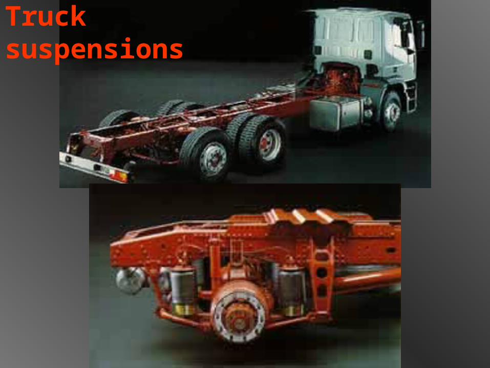
Truck suspensions
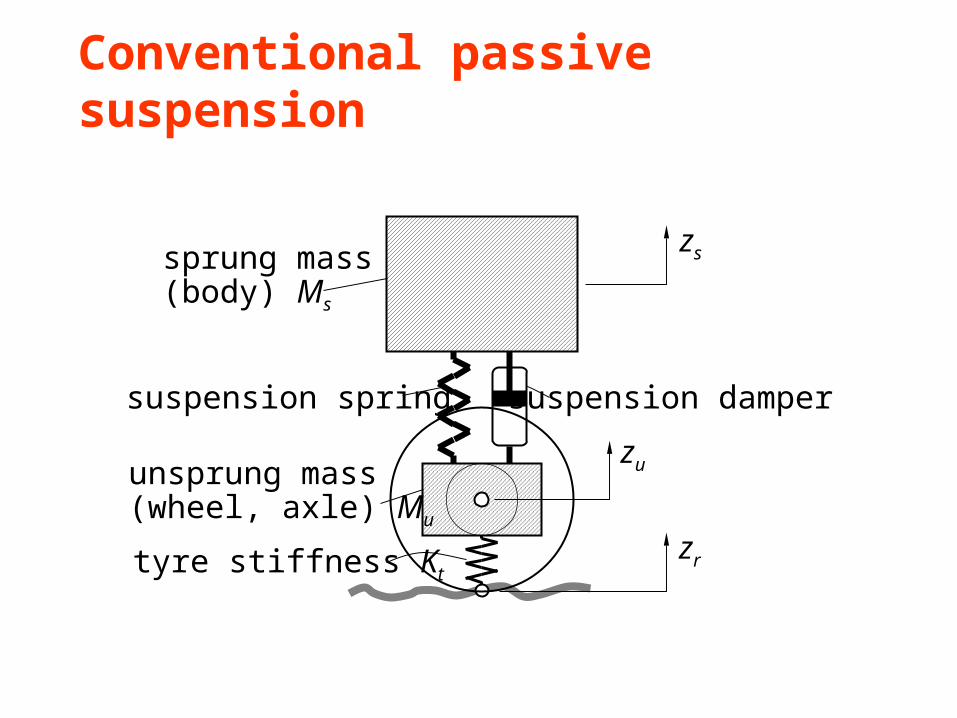
Conventional passive suspension
zs
zu
zr
suspension spring suspension damper
tyre stiffness Kt
sprung mass(body) Ms
unsprung mass(wheel, axle) Mu
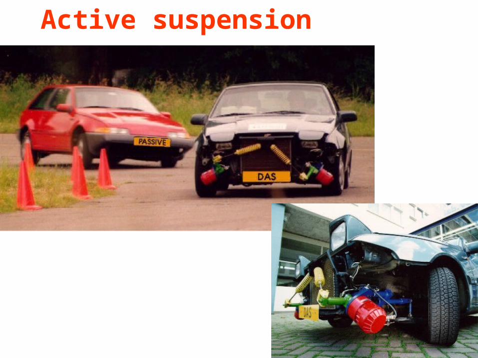
Active suspension
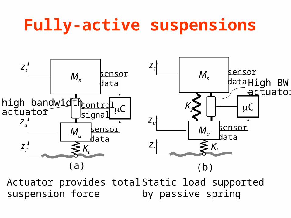
Fully-active suspensions
Ms
zs
zu
zr
C
Mu
Kt
high bandwidthactuator
controlsignal
sensordata
sensordata
(a)
Actuator provides totalsuspension force
Ms
zs
zu
zr
C
Mu
Kt
High BWactuator
sensordata
sensordata
Ks
(b)
Static load supportedby passive spring
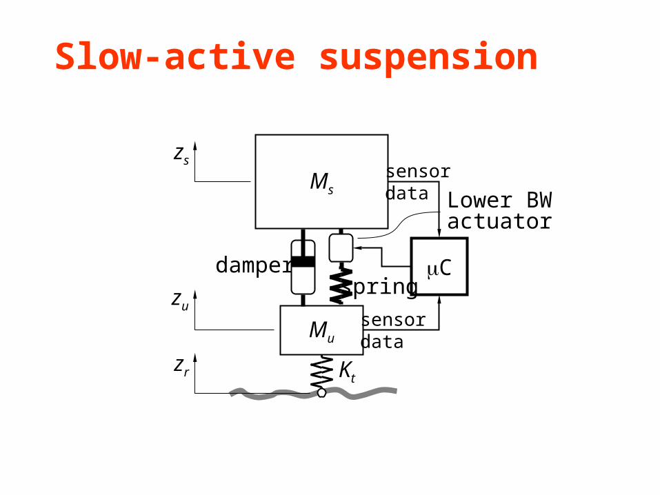
Slow-active suspension
Ms
zs
zu
zr
C
Mu
Kt
Lower BWactuator
sensordata
sensordata
springdamper
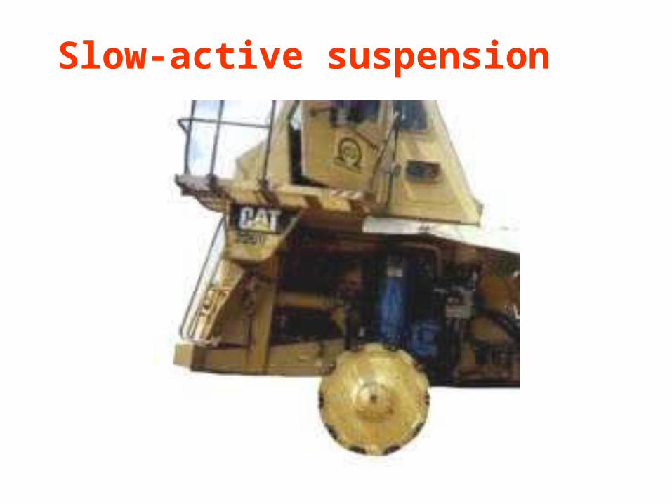
Slow-active suspension
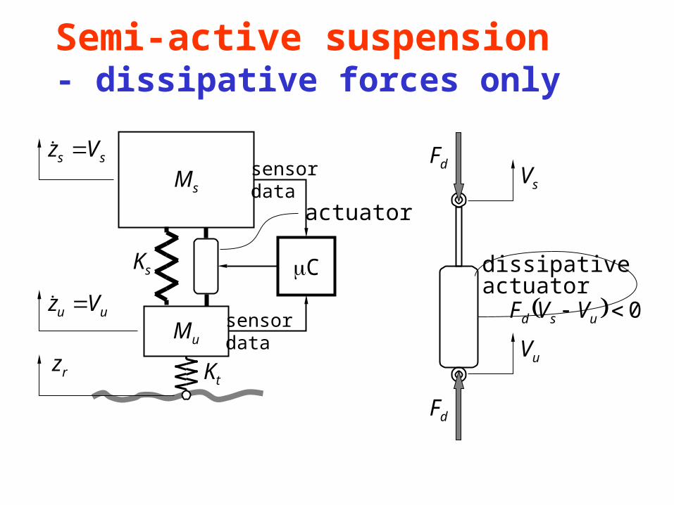
Semi-active suspension- dissipative forces only
Ms
C
Mu
Kt
actuator
sensordata
sensordata
Ks
ss Vz
uu Vz
zr
Fd
Fd
Vs
Vu
dissipativeactuator
0 usd VVF
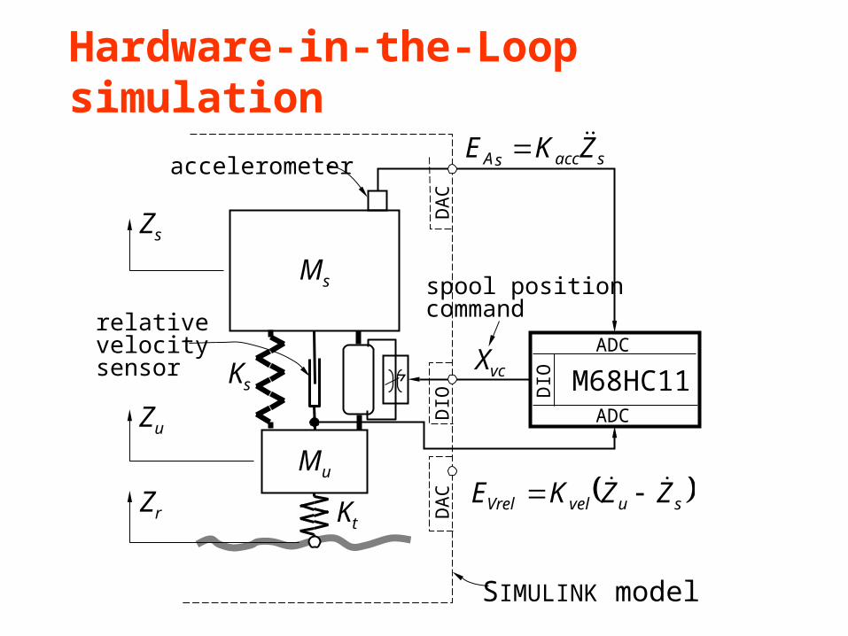
Hardware-in-the-Loop simulation
Ms
Mu
Kt
Ks
Zr
M68HC11ADC
DIO
ADC
DA
CD
AC
DIO
Zu
Zs
Xvc
saccsA ZKE
suvelVrel ZZKE
accelerometer
relativevelocitysensor
spool positioncommand
SIMULINK model
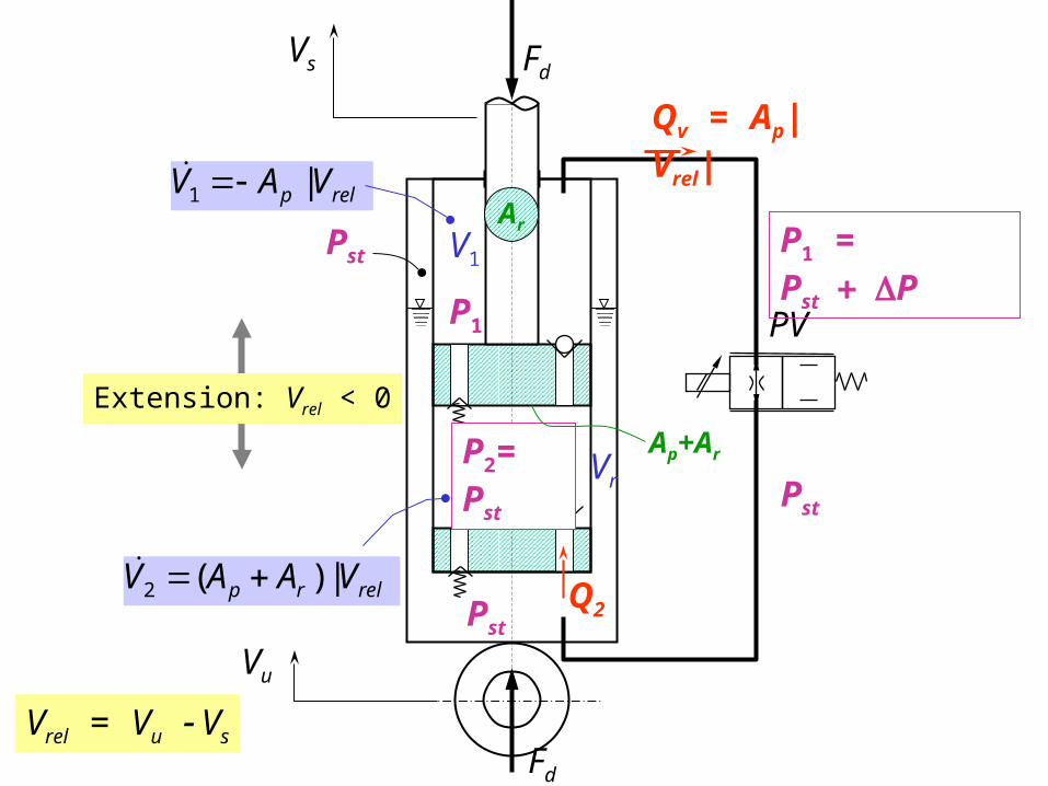
P2
Pst
V1
V2
PV
Vr
Fd
Fd
Q2
P1
P2= Pst
Vs
Extension: Vrel < 0
Qv = Ap|Vrel|
Pst
Vu
Pst
||1 relp VAV
||)(2 relrp VAAV
P1 = PstP
Vrel = Vu Vs
Ar
Ap+Ar
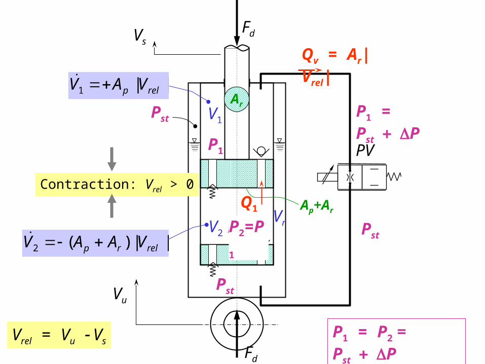
P2
Pst
V1
V2
PV
Vr
Fd
Fd
Q1
P1
Vs
Qv = Ar|Vrel|
Pst
Vu
Pst
||1 relp VAV
||)(2 relrp VAAV
P1 = PstP
Vrel = Vu Vs
Ar
Ap+Ar
Contraction: Vrel > 0
P1 = P2 = PstP
P2=P1
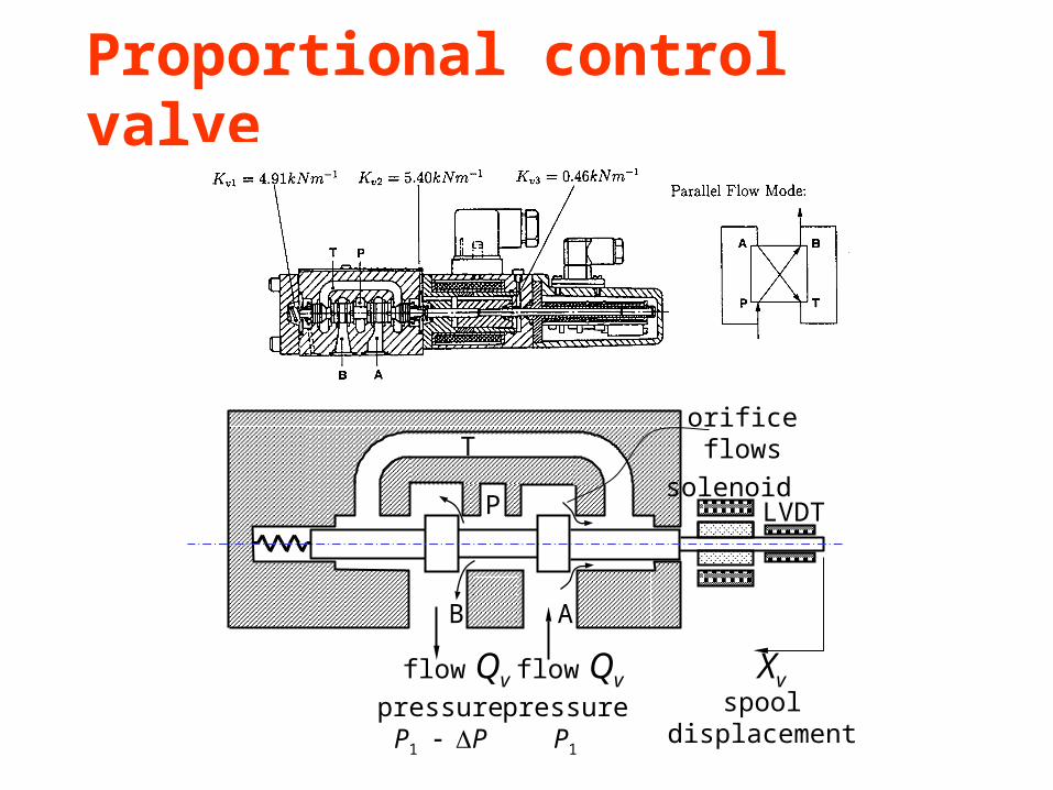
Proportional control valve
P
AB
flow Qv flow Qv
pressureP1 P
pressureP1
Xvspool
displacement
Torificeflows
solenoidLVDT
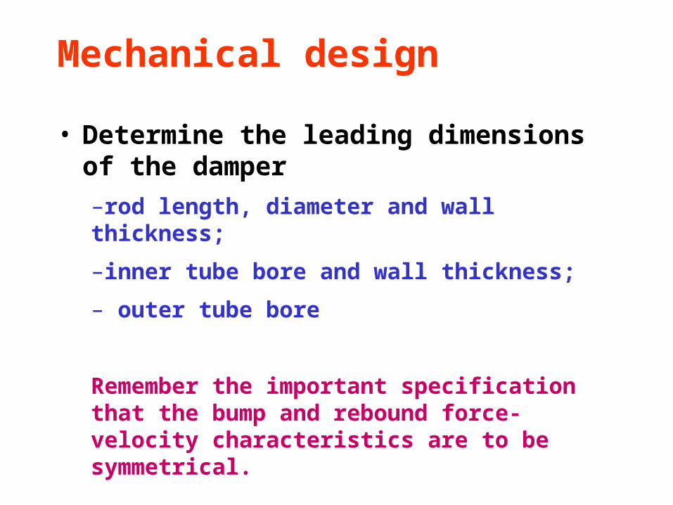
Mechanical design
• Determine the leading dimensions of the damper
–rod length, diameter and wall thickness;
–inner tube bore and wall thickness;
– outer tube bore
Remember the important specification that the bump and rebound force-velocity characteristics are to be symmetrical.
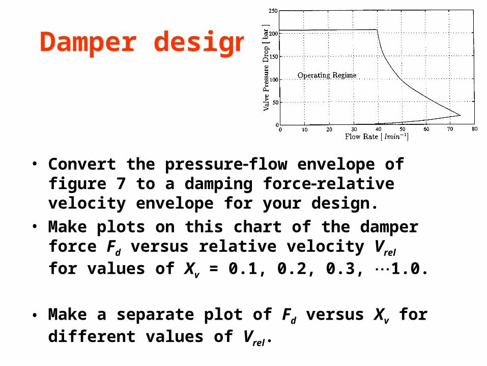
Damper design
• Convert the pressureflow envelope of figure 7 to a damping forcerelative velocity envelope for your design.
• Make plots on this chart of the damper force Fd versus relative velocity Vrel for values of Xv = 0.1, 0.2, 0.3, 1.0.
• Make a separate plot of Fd versus Xv for different values of Vrel.
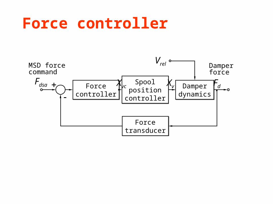
Force controller
Forcecontroller
Forcecontroller
Spoolposition
controller
Spoolposition
controller
DamperdynamicsDamper
dynamics
Forcetransducer
Forcetransducer
Xvc Xv FdFdsa
MSD forcecommand
Damperforce
Vrel
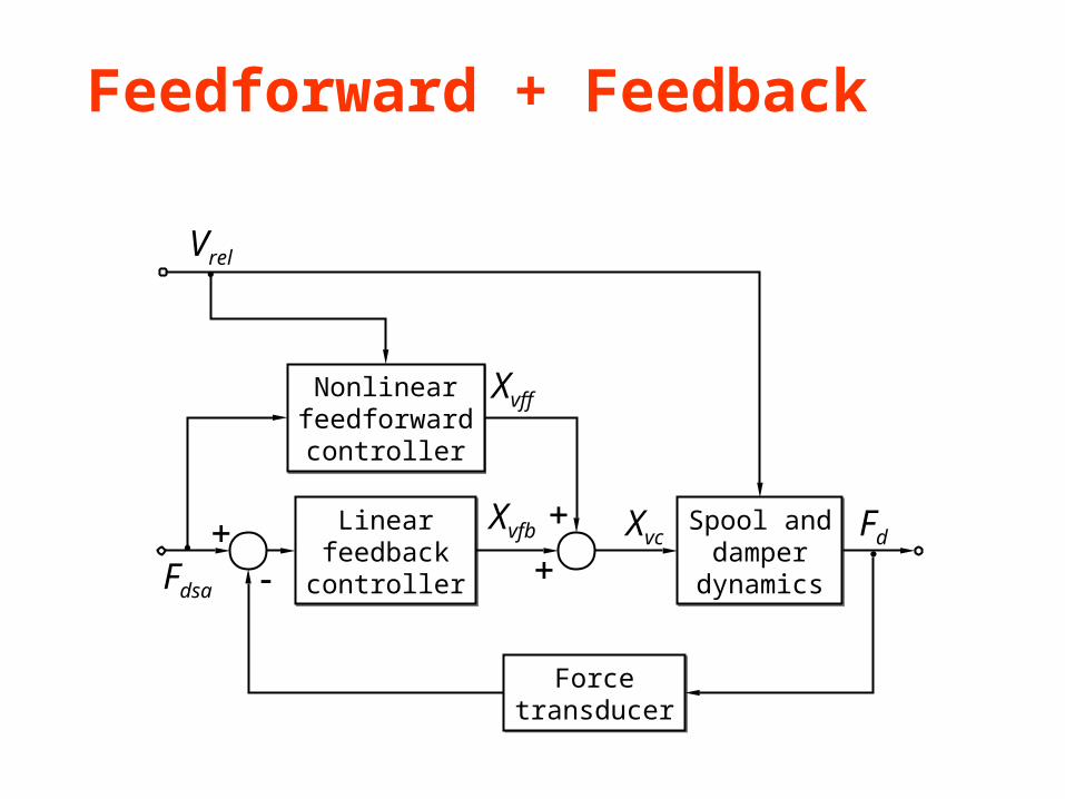
Feedforward + Feedback
Linearfeedbackcontroller
Linearfeedbackcontroller
Spool anddamper
dynamics
Spool anddamper
dynamics
Forcetransducer
Forcetransducer
Xvfb Xvc Fd
Fdsa
Vrel
Nonlinearfeedforward
controller
Nonlinearfeedforward
controller
Xvff
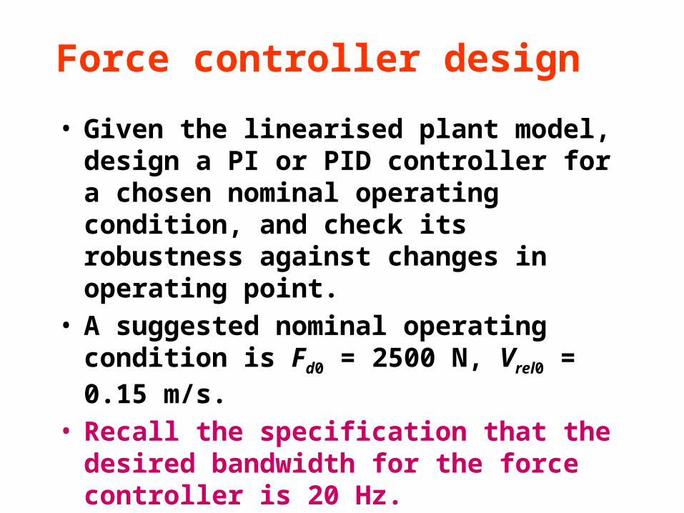
Force controller design
• Given the linearised plant model, design a PI or PID controller for a chosen nominal operating condition, and check its robustness against changes in operating point.
• A suggested nominal operating condition is Fd0 = 2500 N, Vrel0 = 0.15 m/s.
• Recall the specification that the desired bandwidth for the force controller is 20 Hz.
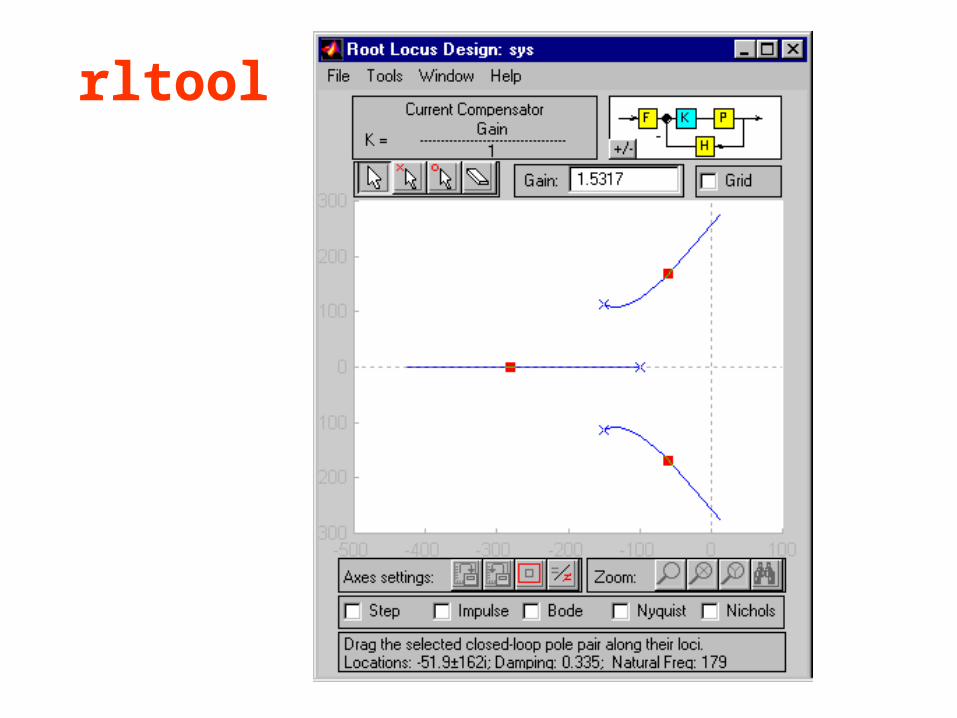
rltool
Alternative controller design
• Use the Ziegler-Nichols ‘ultimate sensitivity’ method to design a PI or PID controller.
• That is, initially set the integral and derivative gains to zero, and increase the proportional gain until the system oscillates on the point of instability.
• Then measure the ‘ultimate gain’ Ku and the ‘ultimate period’ Pu, and apply the tuning rules to obtain a first-cut set of values for the controller gains.
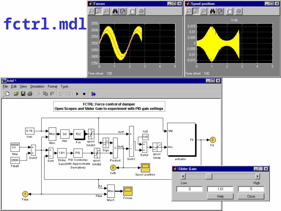
fctrl.mdl
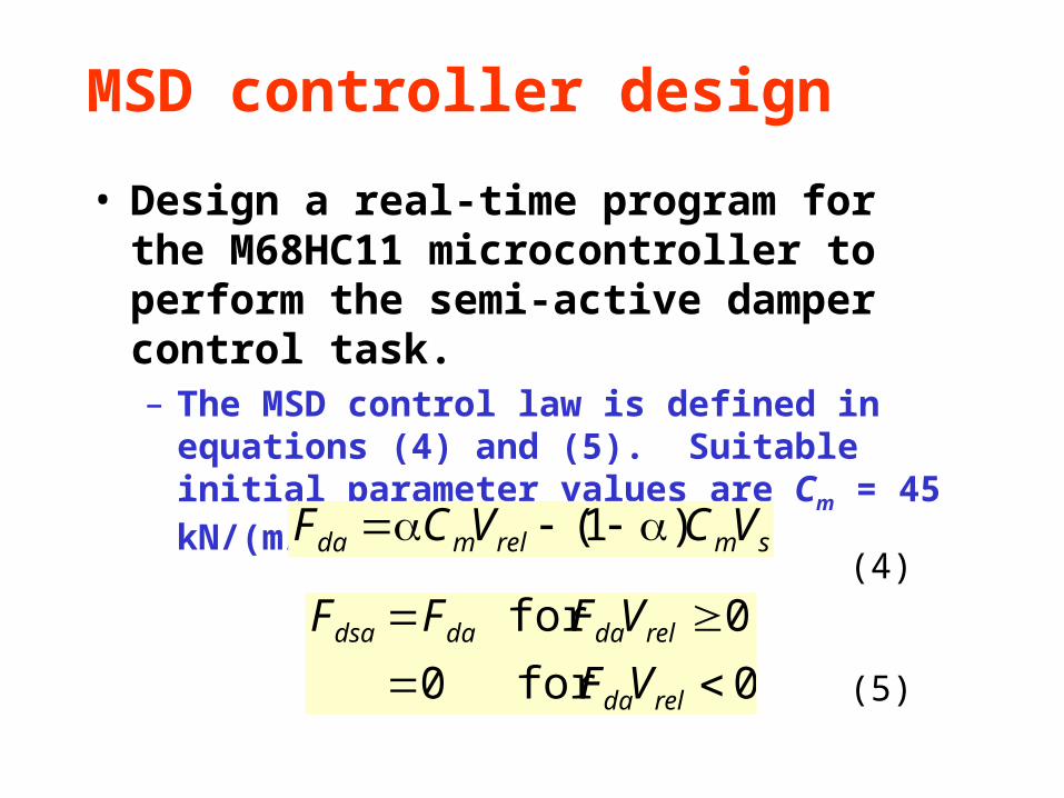
MSD controller design
• Design a real-time program for the M68HC11 microcontroller to perform the semi-active damper control task. – The MSD control law is defined in equations (4)
and (5). Suitable initial parameter values are Cm = 45 kN/(m/s) and = 0.2.
smrelmda VCVCF )1(
0for 0
0for
relda
reldadadsa
VF
VFFF(4)
(5)
Implementation
• Then implement your program in a hardware-in-the-loop simulation, using the SIMULINK model HiL_sys provided. – The roadway roughness input can be selected
to be deterministic (e.g., sinusoidal corrugations) or random (corresponding to a road profile that could be encountered on a main road at 70 km/h).
– Time histories of simulation variables will be written into the MATLAB workspace, so that the performance of the controller can be assessed.
Design tools provided
• SIMULINK model, SIM_sys– This is identical with HiL_sys, except that a
subsystem block M68HC11 is included as a representation of the microcontroller.
– You can modify this block to create your own SIMULINK representation of your controller code, to test its operation before attempting the HiL simulation.
• Ziegler-Nichols tuning tool fctrl
– invoke with fctrl_start
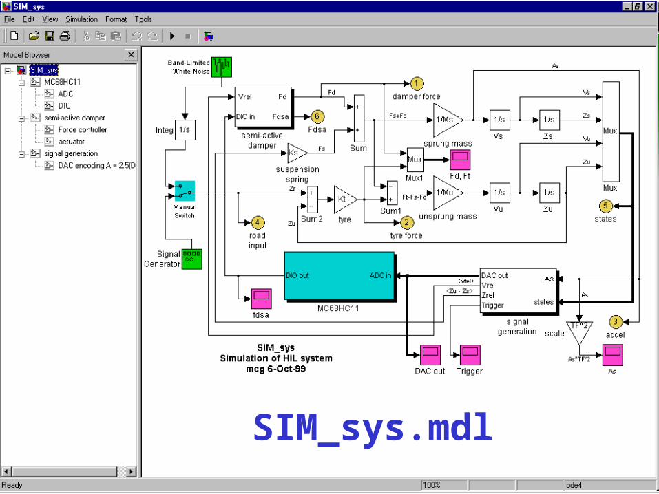
SIM_sys.mdl
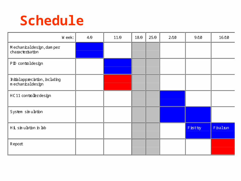
ScheduleWeek: 4/9 11/9 18/9 25/9 2/10 9/10 16/10
Mechanical design, dampercharacterisation
# # # # # # #
PID control design # # # # # # #
Initial appreciation, includingmechanical design
# # # # # # #
HC11 controller design # # # # # # #
System simulation # # # # # # #
HiL simulation in lab # # # # # First try Final run
Report # # # # # # #
PID controllers• PID = Proportional + Integral + Derivative
• Also known as "three-term controller"
• About 90% of all control loops are closed with some form of PID controller
• In this group of lectures we will find out:
– why PID controllers are used so often
– ways of "tuning" a PID controller
– how to deal with actuator saturation
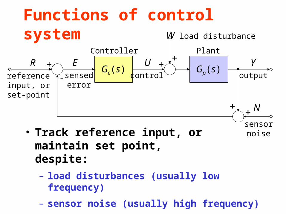
Functions of control system
• Track reference input, or maintain set point, despite:
– load disturbances (usually low frequency)
– sensor noise (usually high frequency)
• Achieve specified bandwidth, and transient response characteristics
Gc(s)Gc(s)
Controller
N
sensornoise
W load disturbance
Gp(s)Gp(s)
Plant
Ucontrol
Youtput
Rreferenceinput, orset-point
Esensed
error
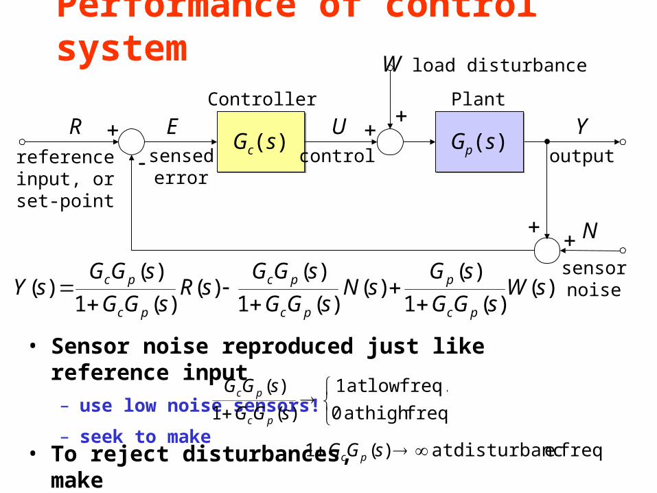
Performance of control system
• Sensor noise reproduced just like reference input
– use low noise sensors!
– seek to make
Gc(s)Gc(s)
Controller
N
sensornoise
W load disturbance
Gp(s)Gp(s)
Plant
Ucontrol
Youtput
Rreferenceinput, orset-point
Esensed
error
)()(1
)()(
)(1
)()(
)(1
)()( sW
sGG
sGsN
sGG
sGGsR
sGG
sGGsY
pc
p
pc
pc
pc
pc
freq. high at
freq. low at
0
1
)(1
)(
sGG
sGG
pc
pc
• To reject disturbances, make freq. edisturbanc at )(1 sGG pc
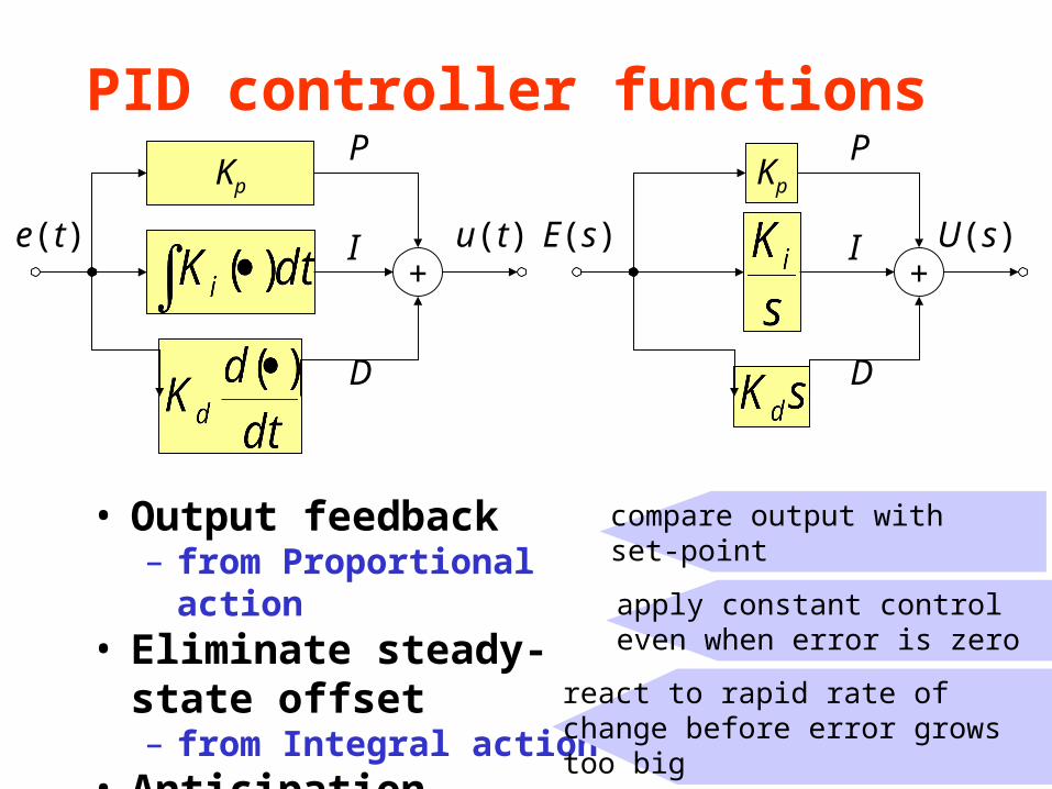
PID controller functions
• Output feedback– from Proportional action
• Eliminate steady-state offset– from Integral action
• Anticipation– from Derivative action
Kp
+
P
I
D
e(t) u(t)
Kp
+
P
I
D
E(s) U(s)
react to rapid rate of change before error grows too big
apply constant control even when error is zero
compare output withset-point
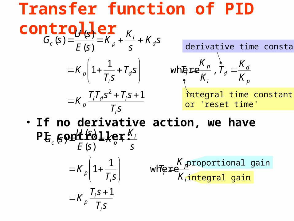
Transfer function of PID controller
sT
sTsTTK
K
KT
K
KTsT
sTK
sKs
KK
sEsU
sG
i
idip
p
dd
i
pid
ip
di
pc
1
, where1
1
)()(
)(
2
integral time constant,or 'reset time'
derivative time constant
• If no derivative action, we have PI controller:
sT
sTK
K
KT
sTK
s
KK
sEsU
sG
i
ip
i
pi
ip
ipc
1
where1
1
)()(
)(
proportional gain
integral gain
-8 -7 -6 -5 -4 -3 -2 -1 0 1 2-5
-4
-3
-2
-1
0
1
2
3
4
5
Real Axis
Imag
Axi
s
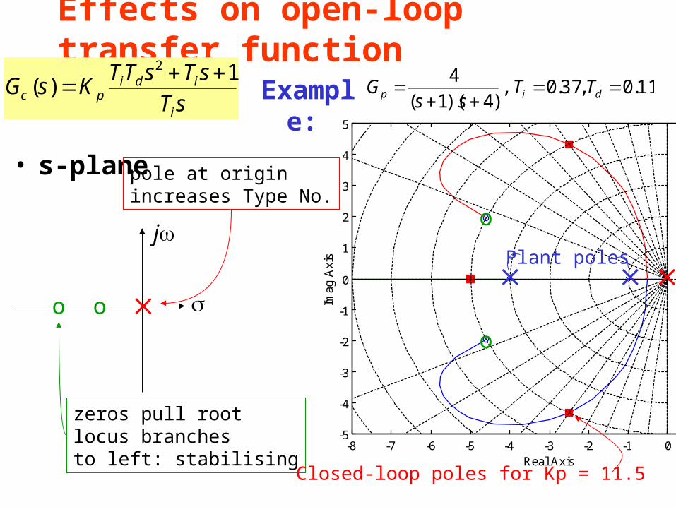
Effects on open-loop transfer function
• s-plane
j
oo
pole at originincreases Type No.
zeros pull root locus branchesto left: stabilising
o
o
Closed-loop poles for Kp = 11.5
Plant poles
Example:
11.0 ,37.0 ,)4)(1(
4
dip TTss
GsT
sTsTTKsG
i
idipc
1)(
2
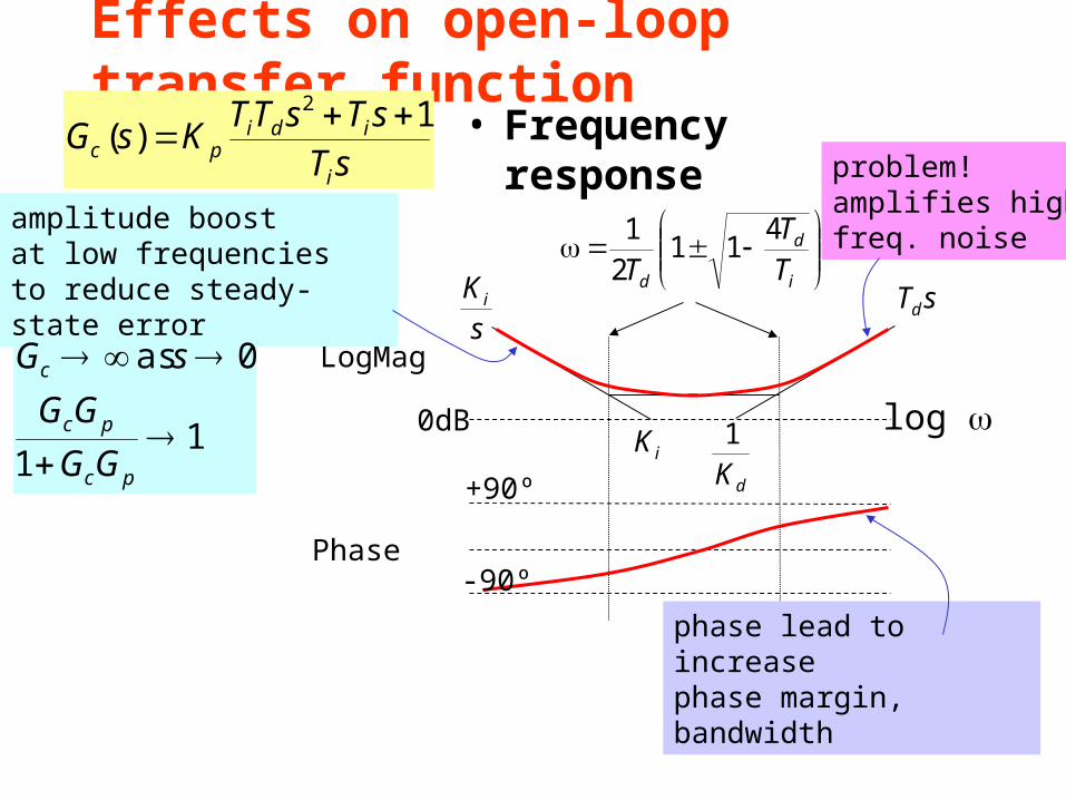
Effects on open-loop transfer function
• Frequency response
0dBiK
dK1 log
s
K i sTd
+90º
-90º
LogMag
Phase
i
d
d T
T
T
411
21
sT
sTsTTKsG
i
idipc
1)(
2
amplitude boostat low frequenciesto reduce steady-state error
phase lead to increasephase margin, bandwidth
11
0 as
pc
pc
c
GG
GG
sG
problem!amplifies highfreq. noise
Application of PID control• PID regulators provide reasonable control
of most industrial processes, provided performance demands not too high
• PI control generally adequate when plant/process dynamics are essentially 1st-order
– plant operators often switch D-action off: "dificult to tune"
• PID control generally OK if dominant plant dynamics are 2nd-order
• More elaborate control strategies needed if process has long time delays, or lightly-damped vibrational modes
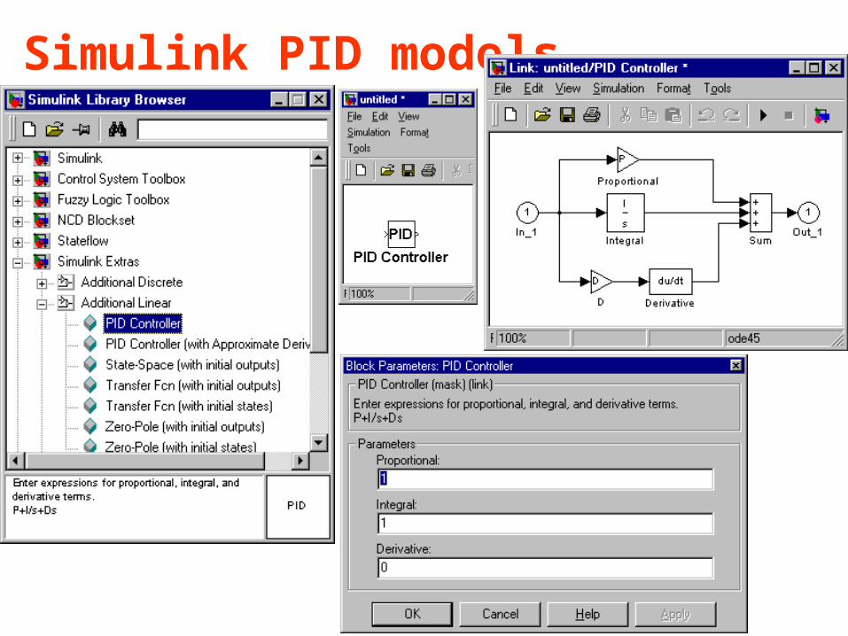
Simulink PID models
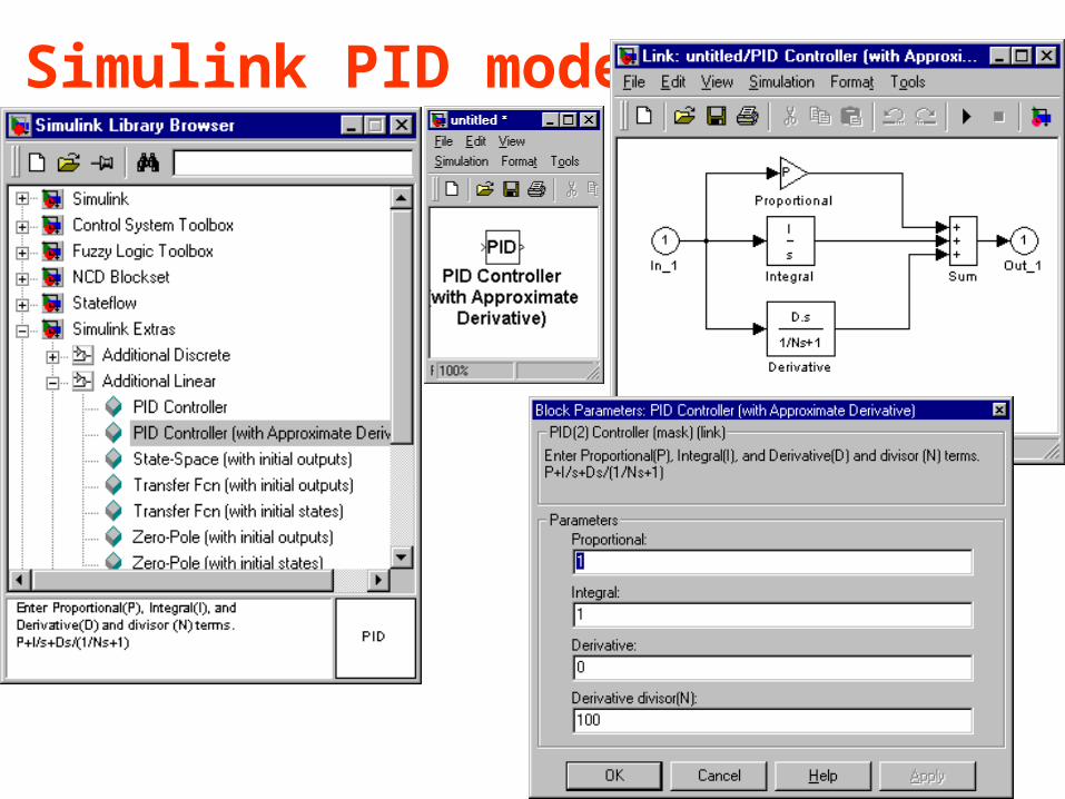
Simulink PID models


