Company Stock Price Reactions to the 2016 Election Shock: Trump, Taxes, and Trade* Forthcoming, Journal of Financial Economics First version: February 1, 2017 This version: August 17, 2017 Alexander F. Wagner 1 Richard J. Zeckhauser 2 Alexandre Ziegler 3 Abstract Donald Trump’s surprise election shifted expectations: corporate taxes would be lower and trade policies more restrictive. Relative stock prices responded appropriately. High-tax firms and those with large deferred tax liabilities (DTLs) gained; those with significant deferred tax assets from net operating loss carryforwards (NOL DTAs) lost. Domestically focused companies fared better than internationally oriented firms. A price contribution analysis shows that easily assessed consequences (DTLs, NOL DTAs, tax rates) were priced faster than more complex issues (net DTLs, foreign exposure). In sum, the analysis demonstrates that expectations about tax rates greatly impact firm values. JEL Classification: G12, G14, H25, O24 Keywords: Stock returns, event study, corporate taxes, trade policy, corporate interest payments, post-news drift, election surprise, market efficiency, price contribution analysis * We particularly thank an anonymous referee and Larry Summers for helpful comments. Wagner thanks the Swiss Finance Institute and the University of Zurich Research Priority Program Financial Market Regulation for financial support. Wagner is chairman of SWIPRA, and an independent counsel for PricewaterhouseCoopers. 1 Swiss Finance Institute – University of Zurich, CEPR, and ECGI. Address: University of Zurich, Department of Banking and Finance, Plattenstrasse 14, CH-8032 Zurich, Switzerland. Email: [email protected]. 2 Harvard University and NBER. Address: Harvard Kennedy School, 79 JFK Street, Cambridge, MA 02139, USA. Email: [email protected]. 3 University of Zurich. Address: University of Zurich, Department of Banking and Finance, Plattenstrasse 14, CH- 8032 Zurich, Switzerland. Email: [email protected].
Transcript
Company Stock Price Reactions to the 2016 Election Shock:
Trump, Taxes, and Trade*
Forthcoming, Journal of Financial Economics
First version: February 1, 2017
This version: August 17, 2017
Alexander F. Wagner1
Richard J. Zeckhauser2
Alexandre Ziegler3
Abstract
Donald Trump’s surprise election shifted expectations: corporate taxes would be lower and trade policies more restrictive. Relative stock prices responded appropriately. High-tax firms and those with large deferred tax liabilities (DTLs) gained; those with significant deferred tax assets from net operating loss carryforwards (NOL DTAs) lost. Domestically focused companies fared better than internationally oriented firms. A price contribution analysis shows that easily assessed consequences (DTLs, NOL DTAs, tax rates) were priced faster than more complex issues (net DTLs, foreign exposure). In sum, the analysis demonstrates that expectations about tax rates greatly impact firm values. JEL Classification: G12, G14, H25, O24 Keywords: Stock returns, event study, corporate taxes, trade policy, corporate interest payments, post-news drift, election surprise, market efficiency, price contribution analysis
* We particularly thank an anonymous referee and Larry Summers for helpful comments. Wagner thanks the Swiss Finance Institute and the University of Zurich Research Priority Program Financial Market Regulation for financial support. Wagner is chairman of SWIPRA, and an independent counsel for PricewaterhouseCoopers. 1 Swiss Finance Institute – University of Zurich, CEPR, and ECGI. Address: University of Zurich, Department of Banking and Finance, Plattenstrasse 14, CH-8032 Zurich, Switzerland. Email: [email protected]. 2 Harvard University and NBER. Address: Harvard Kennedy School, 79 JFK Street, Cambridge, MA 02139, USA. Email: [email protected]. 3 University of Zurich. Address: University of Zurich, Department of Banking and Finance, Plattenstrasse 14, CH-8032 Zurich, Switzerland. Email: [email protected].
1. Introduction The election of Donald J. Trump as the 45th President of the United States of America on
November 8, 2016 surprised most observers. The election’s unexpected outcome (on the
morning of Election Day, Trump’s chances were 17% on Betfair and 28% on FiveThirtyEight)
combined with the wide policy differences between the two candidates led to substantial
reactions on financial markets. Large price moves were recorded across asset classes, including
stocks, bonds, and exchange rates.
This paper focuses on the response of stock prices to the election in the short- and in the
longer run. Assessing the relative winners and losers among companies from the election is
interesting, given the sizable differences in the policies the two candidates favored in several
economically important areas. One major difference, a prime focus of this paper, lay in expected
corporate tax policy changes. While dividend taxes have changed frequently, leading to a large
literature on the effects of dividend taxes on stock prices (reviewed in Graham, 2003, and
Hanlon and Heitzman, 2010), the last major US federal corporate tax reform dates back to 1986.
Thus, although corporate finance theory suggests a first-order effect of corporate taxes on firm
value, it has not been possible recently to study the actual pricing of federal tax changes. The
2016 Presidential election provides a unique opportunity to conduct such an analysis because it is
rare in developed economies to have the combination of such a surprising outcome and such a
difference in tax policies between the candidates.1 We take advantage of these two
characteristics of the event to investigate first the impact of taxes on firm value, and second the
efficiency of stock price responses to potentially dramatic changes in both the corporate tax rate
and other important features of the tax system.
The 2016 Presidential election has unique advantages and disadvantages compared to events
analyzed in other papers examining stock price responses to changes or expectations about
changes in tax policy. In such events, such as the 2003 Dividend Tax Cut (Auerbach and Hassett,
2006, 2007; Amromin, Harrison, and Sharpe, 2008), the proposed policy change is usually
known with some precision and little else is involved during the event window; these are
1 There is a large general literature on the effect of elections on financial markets. For example, Niederhoffer, Gibbs, and Bullock (1970) consider Dow Jones Industrial Average responses to elections and nominating conventions. Moreover, a substantial literature studies the stock market development during Democratic and Republican administrations over the longer run. For example, Santa-Clara and Valkanov (2003) document a “presidential premium” (especially for large-cap stocks) during Democratic presidencies. Knight (2007) studies stock prices of 70 politically sensitive firms and election odds in a prediction market in the run-up to the Bush/Gore election of 2000.
1
advantages. A typical disadvantage is that the surprise of the event is low since the probability of
the policy passing is generally reasonably high. Moreover, the outcome if it does not pass is
unknown, as a modified policy may be adopted if the initial proposal fails. These advantages and
disadvantages are reversed in the case of the 2016 election. Trump’s election affected
expectations about many things besides corporate tax policy, a disadvantage, and as we discuss
below, the specific tax policy that would ultimately be implemented, if any, was uncertain.
However, the election surprise was large, an advantage, and the alternative policy – maintenance
relatively close to the status quo for corporate taxes under a Clinton presidency with a
Republican majority in the House – was reasonably clear.
Many policies, and in particular tax policies, require Congressional approval. Thus, rather
than Trump’s election per se, it is probably the fact that Republicans controlled both the
Presidency and Congress after the election that led investors to expect substantial corporate tax
reform to be much more likely than under alternative election outcomes. Either a Clinton
presidency and/or a Democratic majority in the Senate would probably have produced gridlock,
similar to the 2010-2016 period, making major policy changes unlikely. Nevertheless, it is
important to keep in mind that there were two Republican corporate tax plans going into the
election – one from the Trump campaign, and one from the House Republicans – and that they
differed on a number of dimensions. While the tax reform that will ultimately be implemented, if
any, will undoubtedly differ significantly from both plans, these two plans constitute the
preponderance of information on possible tax reform options that was available to investors at
the time of the election and thereafter. The one-page description of the Administration’s intended
plan on April 26, 2017 (The White House, 2017) provided an update. That intended plan
incorporated important elements from both the Trump-campaign plan and the House
Republicans’ plan. It is therefore useful to summarize those plans’ main elements to guide the
analysis conducted in this paper.
Among the noteworthy elements of Trump’s campaign plan (Trump, 2016) are: (i) a
reduction in the statutory corporate income tax rate to 15% from the current 35%; (ii) a one-time
deemed repatriation of corporate cash held overseas at a 10% tax rate, followed by an end to the
deferral of taxes on corporate income earned abroad (with the current combination of worldwide
2
taxation and foreign tax credits being maintained);2 and (iii) an election available to firms
engaged in manufacturing in the U.S. to immediately expense (rather than depreciate) capital
investment. However, firms that elected expensing would not be allowed to deduct interest
expenses.
The House Republicans’ tax plan (Republicans, 2016) contained the following elements: (i)
a reduction in the statutory corporate income tax rate to 20%; (ii) immediate expensing of
business investments in both tangible and intangible assets (with the exclusion of land); (iii) the
elimination of deductibility of net interest expense (although interest expense would be
deductible against interest income); (iv) the addition of an interest factor to net operating loss
(NOL) carryforward balances that compensates for inflation and a real return on capital,
associated with a removal of NOL carrybacks, and the introduction of an annual limitation on
NOL utilization equal to 90 percent of pre-NOL taxable income; (v) the introduction of border
adjustments that exempt exports and tax imports; (vi) a switch to a territorial taxation system;3
and (vii) the taxation of accumulated foreign earnings at a rate of 8.75% if held in cash or cash
equivalents and at 3.5% otherwise (with companies able to pay the resulting tax liability over an
eight-year period).
Thus, the two corporate tax plans agree on three critical elements: dramatic reduction in the
federal statutory rate from its current level of 35%, the expensing of capital expenditures with a
limitation on interest expense deductibility, and an announced intention to tax accumulated
foreign earnings. However, the plans differ on the issues of border adjustment, territorial versus
worldwide taxation, and NOL rules (which the Trump plan did not address). Importantly, some
aspects of both plans affect multinationals differently from purely domestic firms. Furthermore,
while Trump’s plan did not include a border adjustment tax, he had repeatedly promoted
introducing or increasing tariffs during the campaign, and hinted at other measures to protect
American industry. Whether a border adjustment tax constitutes a fundamentally different
approach to corporate taxation or a tariff is subject to debate. However one views this issue, a
central fact remains: trade and tax policy are closely intertwined and a differential impact of the
2 Under the current tax regime, firms are taxed on worldwide income but that tax can (with a few exceptions) be deferred until the foreign subsidiaries distribute the monies back to their US parent. When repatriating foreign profits, firms get a credit for the foreign taxes paid on that income. The end of deferral was mentioned in the original version of the Trump campaign tax plan (Trump, 2015) but not discussed in his revised plan (Trump, 2016); however, since the revised plan did not mention a switch to territorial taxation, it appears to be reasonable to assume that the worldwide taxation/foreign tax credit system would be maintained. 3 Under a territorial taxation system, dividends received from foreign subsidiaries are exempted from US taxation.
3
election on purely domestic firms and multinationals is to be expected. While we show this
differential impact, we are agnostic as to what extent it is driven by tax policy or trade policy.
Guided by the provisions of these plans, we investigate the differential performance of
Russell 3000 stocks along a number of tax-related dimensions to determine which factors
produced relative winners and relative losers among companies in the time period from the
election to the end of April 2017 (the one-hundred-day mark of the Presidency). These results
shed some light on the effect of expectations about tax policy on individual firms. In addition to
establishing what factors affected stock returns, we investigate the speed with which markets
processed information related to the different dimensions. Studying how rapidly these
expectations were incorporated into market prices is particularly informative in light of the
market upheaval right after the election results became known.4
We find strong evidence that expectations of a major corporate tax cut substantially
impacted the cross-section of stock returns. Specifically, firms with high effective tax rates (both
cash ETR and GAAP ETR)5 and large deferred tax liabilities benefited, while those with
deferred tax assets resulting from NOL carryforwards lost. The stock market’s reactions through
end of April 2017 also imply that expectations about the effects of the incoming administration’s
anticipated policies for internationally oriented firms were negative, perhaps reflecting fears of
retaliatory tariffs or trade barriers from other nations, perhaps reflecting expectations of an
unfavorable tax treatment for foreign earnings. Investors also downgraded companies with high
leverage and high interest expenses. By contrast, the level of capital expenditures did not affect
the cross-section of stock returns, suggesting that investors thus far think that expensing capital
investments is either unlikely to be implemented, or of secondary consequence.
4 While the changes of prices of some assets were consistent with what had been forecast if Trump were to win (e.g., the Mexican Peso, Latin American and Pacific Rim stock markets), others moved in the opposite direction (e.g., US stocks and Treasuries). This occurred even though the forecasts had a strong empirical foundation. For instance, in a study of asset price moves during the first Presidential debate on September 26, 2016, Wolfers and Zitzewitz (2016) find a strong positive relation between the odds of Clinton winning on Betfair and the returns on all major US equity index futures and a negative relation for Treasury futures. While stock index futures fell sharply on election night as the outcome of the election became known, stock markets finished up on the day following the election, and rallied strongly during the rest of the year and beyond. Treasuries rose sharply on election night but then declined significantly until year-end. 5 The cash ETR is the ratio of cash taxes paid (available as a separate disclosure at the bottom of the statement of cash flows) to pretax income. The GAAP ETR is the ratio of the provision for income taxes (the total income tax expense computed following GAAP rules reported in the income statement) to pretax income; its value is also disclosed separately in the notes to firms’ financial statements. Hanlon and Heitzman (2010) provide a detailed description of these measures and a discussion of their respective advantages.
4
All these findings hold whether data is used in any of three traditional forms: raw returns,
returns adjusting for market moves,6 and returns adjusting for the Fama-French size and value
factors. After controlling for size and value, corporate taxes explain somewhat less of abnormal
returns. As we show, this is the case because high-tax firms load more on these factors.
Interestingly, markets digested information on these various aspects at varying speeds. To
study the speed of price adjustment, we introduce the price contribution methodology commonly
used in the market microstructure literature to the empirical corporate finance literature.
Specifically, using daily cross-sectional regressions, we quantify the additional price impact of
the different variables on each of the first ten trading days after the election. In that time window,
no material new information regarding upcoming policies became known, making this period an
ideal setting to study the speed at which markets processed publicly available information. Of all
the variables considered, deferred tax liabilities affected returns fastest in terms of the first-day
price impact – 80% of their price impact occurred on the first day. Next fastest were deferred tax
assets from NOL carryforwards. Interestingly, net deferred tax liabilities (whose effect is
difficult to assess for reasons that we discuss in greater detail below) were slowest. The effects of
firm leverage, interest expense, foreign exposure, and both cash and GAAP ETRs were priced in
modestly on the first day. None exceeded 30% of its ten-day effect. Thus, like most of the
literature on price responses, we find evidence of delayed incorporation of public information
into prices.
While this price contribution analysis reveals how long it took prices to reach their ten-day
response, it does not measure the speed at which price uncertainty declined. To assess that speed,
we conduct an additional analysis for variances rather than for returns. Again, we find sizable
differences in the speeds at which prices along the different dimensions converged towards their
ten-day levels. Deferred tax liabilities and deferred tax assets from NOL carryforwards
converged most swiftly; net deferred tax liabilities converged the slowest. ETRs, leverage,
interest expense, and foreign exposure closed in at an intermediate pace.
This analysis presents intriguing evidence of the efficiency with which the market
responded, in particular differences in efficiency across dimensions. To demonstrate those
differences required a methodological innovation. To our knowledge, a price contribution
6 Since the stock market was up so dramatically, many relative losers actually gained in price, but not nearly so much as relative winners.
5
analysis, such as ours, has not been done for coefficients from a cross-section of stock price
reactions. This method has the potential to be employed in a range of other settings.7
The Internet Appendix shows that high-tax firms outperformed low-tax firms on days when
media coverage of tax reform was high (such as when the elements of tax reform were
announced on April 26, 2017), but that taxes played no role in explaining stock price reactions to
other salient non-tax-relevant events (such as the imposition of a travel ban to the US from a
group of countries).
In a separate section, we address a cluster of consequential happenings beyond the one-
hundred-day mark. In mid May 2017, in the wake of the firing of FBI Director Comey, President
Trump experienced a slew of adverse news stories about developments that sharply increased the
probability of impeachment and cut the probability of a tax cut, as indicated by prices on
political betting markets. All major US equity indices plunged on May 17. While not nearly as
dramatic an event as the surprise election, we find that the market interpreted these troubles as a
signal of a less likely, delayed and/or smaller tax cut, with high-tax firms strongly
underperforming low-tax firms.
In sum, beyond showing that stock prices reacted in the expected direction to Trump’s
election and his first one hundred days in office, the results also demonstrate the varying speeds
with which different aspects regarding corporate taxes and trade issues were reflected in prices.
Most broadly, this relatively clean natural experiment confirms that expectations about tax rates
greatly impact firm values.
2. Asset price responses to news If the market responds optimally to an election outcome, the change in the market price of
any asset will reflect both the difference in its expected discounted payoff between the two
possible outcomes and the ex ante probability that that outcome occurs. The advantage of
considering asset price changes is that they capture current expectations; the researcher need not
trace all the future changes to cash flows and discount rates separately (Schwert, 1981).
Formally, let Pn be the price of asset n prior to the 2016 election, and let Pn,C and Pn,T denote the
7 When examining the speed of pricing of a piece of news pertaining to a company, the corporate finance literature typically checks whether the drift over different horizons after some initial reaction can be explained by that variable, but does not differentiate between return and variance contribution, and does not compare the speed with which different pieces of news (or different exposures of firms to a given piece of news) get impounded into prices.
6
expected price of the asset conditional on Clinton and Trump winning, respectively. Let πC and
πT = 1 – πC be the probabilities of the two outcomes. Ignoring discounting over the short period
involved, and assuming that risk aversion is a minor factor,8 the asset’s price before the election
is given by
TnTCnCn PPP ,, ππ += . (1)
The price change for the asset given that Trump won is given by
)1)(( ,,, TCnTnnTnn PPPPP π−−=−=∆ . (2)
In words, the price change once the election results become known is the difference in prices
between the two outcomes, times the size of the election surprise, which in turn is one minus the
ex ante probability of Trump winning. For instance, had Trump’s election been certain ex ante,
there would not have been a price reaction on the day after the election. Scaling this expression
by the initial price, the return on the asset once the election results become known is given by
n
TCnTn
n
nTnn P
PPP
PPR
)1)(( ,,, π−−=
−= . (3)
Note that while the election surprise is the same for all assets, individual assets will respond
to the election outcome differently, depending on the sign and magnitude of the spread between
Pn,C and Pn,T for those assets. For assets that would have benefitted from a Clinton outcome
relative to Trump, Pn,C > Pn,T, with the inequality reversed for assets that would be helped by a
Trump outcome. To presage some of our findings, stocks reacted very differently to the outcome,
holding fixed the overall market reaction. By examining the cross-section of stock returns, we
can infer whether the incoming administration’s expected policies were viewed as favorable or
unfavorable for a particular firm or industry, and can then assess the extent and speed with which
markets incorporated differences between the candidates on different policy dimensions into
prices.
The 2016 Presidential election has two major advantages for an event study over events the
literature typically considers. First, there was a significant gap between the pre-election
probabilities and the election outcome. Clinton was the strong favorite on betting markets, in
polls, and on election-modeling websites. For instance, on November 7, the probability of
Clinton winning on Betfair was 83%, while on the day of the election, even the FiveThirtyEight
8 Risk aversion on overall market movements would, of course, be reflected in beta. Stocks expected to perform better in an unfavorable overall outcome would be priced higher and vice versa.
7
forecast, which was the major site that gave Trump the highest probability of winning, put the
Clinton odds between 71% and 72%. Second, there were major differences between the policies
favored by the two candidates. This combination explains why stock prices responded so
strongly.
As mentioned in the Introduction, the event also has two disadvantages: it affected
expectations about many things besides corporate tax policy, and the specific tax policy that
would be proposed was not yet known with precision.
Although the election outcome reduced uncertainty about firms’ prospects, substantial
uncertainties remained for a number of reasons. First, the elected candidate was expected to
backtrack on some pledges he made on the campaign trail, even some made repeatedly, or to
change his mind on intended policies or the strength with which he would pursue them. Second,
many policies would need Congressional approval. Although the Republicans controlled
Congress, their majority in the Senate was merely a slender two, and a number of Republican
senators disliked Trump and/or some of his policies. Thus, he might push policies, but Congress
might not approve. Accordingly, the specific design and perceived probabilities of various
policies being implemented remained subject to large shifts after the election results were
known. Thus, sizable relative asset-price reactions could be expected in the weeks and months
that followed. We therefore proceed in two steps: First, we illustrate which factors mattered
immediately and for the overall stock return of a company in the first one hundred days of
Trump’s administration. Second, we examine the first ten days after the election, when arguably
little shift in the perception of probabilities of implementation and the content of tax reform took
place. This approach allows a relatively pure analysis of the speed of information processing.
3. Data and empirical strategy Our empirical strategy regresses abnormal returns (ARs) on firm characteristics. Since
markets often need time to digest new information, and further information on the incoming
administration’s proposed policies became clearer only after the election, we consider different
sets of abnormal returns: those on the day after the election, the drift from two days after the
election to ten trading days (two business weeks) after the election, the cumulative returns
through year-end (with December 30 as the last trading day), and then through the end of two
two-month periods, until February 28 and April 28, 2017. These analyses shed light on both the
8
overall reaction and the speed with which the market reacted. We note that the end of April 2017
is a somewhat arbitrary end point, but the oft-cited one-hundred-days-in-office mark (which
occurred on the weekend, April 29, 2017) does make for a natural focus to assess the market’s
responses to the Trump Presidency.
Our sample includes the Russell 3000 constituents as of the day of the election.9 Together,
the index constituents represent roughly 98% of the U.S. equity market capitalization. We
exclude 142 companies whose initial stock prices were below US$5.
We obtain stock prices adjusted for splits and net dividends from Bloomberg. We conduct
all of our analyses using two sets of abnormal returns: one set calculated with respect to the
CAPM, and another employing the Fama-French three-factor model. To obtain CAPM-adjusted
returns, we first compute each stock’s market beta from an OLS regression of daily stock returns
in excess of the risk-free rate on the excess returns on the Russell 3000 total return index for the
period from September 30, 2015 to September 30, 2016 (estimation window).10 The risk-free
rate is the one-month T-bill rate.11 We then compute abnormal returns for all days surrounding
the November 8, 2016 election as the daily excess return on the stock minus beta times the
Russell 3000 excess return. To compute Fama-French-abnormal returns, we obtain daily data for
the market excess return, the size and value factor returns, and the riskless rate from Ken
French’s website. We then estimate each stock’s factor betas from an OLS regression of its
excess return on the market, size, and value factors over the estimation window. Finally, we
obtain each stock’s abnormal returns as its excess returns minus the sum of its factor exposures
times the factor returns. Throughout the paper, all returns are reported in percentage points.12
Fig. 1 plots some quantiles of the distributions of equally weighted CAPM-adjusted returns
around the election. It indicates substantial variability in the way different firms’ stock prices
9 The Russell 3000 actually had 2,966 members as of November 8, 2016. A number of firms leave the sample over time due to acquisitions (72 cases by April 28, 2017) and bankruptcy (one case in April 2017). 10 Data are available for the entire estimation window for 2,842 out of the 2,966 firms. The 124 other firms have a short return history, mostly because they result from spin-offs and met the index inclusion criteria soon after their first trade date. An example is Hewlett Packard Enterprise Company, which was spun off from HP Inc. on November 2, 2015 and entered the index on that same date. Beta for 117 of these firms is estimated using returns from the date the firm was first traded to September 30, 2016. The return history for the remaining seven firms begins after September 30, 2016, so no beta estimates and no abnormal returns are computed for them. 11 The results are virtually identical if we use the returns on the Russell 3000 price index instead of those on the total return index and/or the Federal Funds rate instead of the T-bill rate. 12 In any empirical analysis, there is the potential that extreme values – possibly due to transcription errors – distort results. Hence, we conduct additional analyses in Section 4.5 with abnormal returns winsorized or trimmed at the 1% and 99% levels. The results prove virtually the same, though statistical significance is often greater.
9
reacted. The positive average and median returns in the few days after the election were due to
the strong performance of small stocks. They notably outperformed large stocks during that
period (the returns on the Fama-French size factor during the three days after the election are
1.89%, 1.12%, and 2.51%). It is noteworthy (though hardly surprising) that the spreads of the
abnormal returns after the election greatly exceed those before. Interestingly, the spread in
abnormal returns remained elevated for about four trading days after the election. By November
15, however, that spread had fallen back to its pre-election level. This result suggests that the
markets needed about four trading days to digest the information associated with the election
outcome. We will return to this issue when we examine market efficiency in Section 5.
-2
0
2
4
Abno
rmal
retu
rns i
n %
Lower quartile Average Median Upper quartile
Nov 7 Nov 8(Election
Day)
Nov 11(Friday)
Nov 15 Nov 18(Friday)
Nov 22
Fig. 1. Abnormal stock returns around the election. This figure shows the equally weighted average, median, and quartiles of CAPM-adjusted returns the day before the election, the day of the election, and the ten trading days after the election.
We obtain explanatory variables mostly from Compustat Capital IQ, and use the most
current accounting data for all companies. For most companies, this means the December 31,
2015 data. However, several companies have fiscal years that end in other months. Thus, we
have 723 companies for which calendar year 2016 data are included.13 The cash effective tax rate
13 Where Compustat data are missing for the most recent year, we replace them with prior-year data. Even among the companies with December 31 as fiscal year end, in mid-February 2017 (the time of download of all public company financials from Compustat) there were already a few companies in Compustat with year-end 2016 data. It
10
(cash ETR) is computed as the percent cash taxes paid relative to current year pretax income
(adjusted for special items).14
When assessing the impact of taxes on the value of a stock, what matters to investors is the
amount in taxes that a company will be paying over several future years. Thus, one question that
arises in the context of our analysis is whether to use the ETR in the year just completed, or an
average rate computed over several years as the explanatory variable. Dyreng, Hanlon, and
Maydew (2008) show that effective tax rates vary substantially over time, and that one-year cash
ETRs are not very good predictors of long-run ETRs. Following their findings, we investigate
whether one-year or longer-term past ETRs are better able to predict future cash ETRs. While
future ETRs are indeed difficult to predict, we find that past one-year ETRs predict future one-
year ETRs better than do past ten-year ETRs (the average of a firm’s total cash taxes paid over a
ten-year period, divided by the sum of its total pretax income (excluding the effects of special
items) over the same ten-year period). Specifically, in data from 1986 to 2016, regressing next
year’s one-year ETR on the current one-year ETR (ten-year ETR) yields regression coefficients
of around 0.3 (0.2) and R2 values of about 20% (10%), depending on the exact implementation.
Therefore, we primarily use one-year ETRs in our analysis. Our main results also hold if the ten-
year ETRs rather than one-year ETRs are employed as explanatory variables, though they are
somewhat weaker for the longer-term return regressions.
The GAAP effective tax rate (GAAP ETR) is an alternative proxy for the tax rate. It uses tax
expenses, instead of cash taxes paid, as the numerator.15 Market value of equity (MVE), deferred
tax assets from net operating loss carryforwards (NOL DTA), deferred tax liabilities (DTL) and
net DTL are from Bloomberg.16, 17
is in principle conceivable that they adjusted their accounting after the election, but a robustness check reveals that using year-end 2015 data yields similar results. 14 As in Dyreng, Hanlon, Maydew, and Thornock (2017), when using this variable, we restrict the sample to those firms with positive pre-tax income (all but 659 companies) as well as a tax rate below 100% (all but 39 companies). The results are robust to not adjusting income for special items. 15 As with the cash ETR, we restrict the sample to firms with positive pre-tax income and a tax rate below 100%. 16 Compustat reports NOL carryforward balances in the field TLCF. However, prior literature has expressed concerns about the quality of Compustat’s NOL data (Mills, Newberry, and Novack, 2003). Our inspection of the data has revealed a few significant errors (amounts being off by a factor of one thousand). Moreover, cross-checking a small sample of data points by hand with 10-Ks reveals that Compustat includes tax loss carryforwards in foreign jurisdictions. The value of those components of tax loss carryforwards would not be directly affected by a US tax cut. However, these carryforwards may proxy for the degree of non-US activities of the company. 17 Deferred tax assets include several components besides DTAs from NOL carryforwards, such as foreign tax credit and R&D tax credit balances. Net deferred tax liabilities, which are defined as deferred tax liabilities minus deferred tax assets, therefore generally differ from DTL minus NOL DTA.
11
Table 1 Descriptive statistics.
This table presents descriptive statistics. The sample includes the Russell 3000 constituents as of November 8, 2016 with stock prices above US$5. Panel A summarizes returns data. Throughout the paper, all returns are reported in percentage points. AR indicates abnormal return, and CAR indicates cumulative abnormal return. CAPM-adjusted returns for all days from November 9, 2016 to April 28, 2017 are computed as the daily excess return on the stock minus beta times the Russell 3000 excess return, where beta is estimated on daily excess returns from September 30, 2015 to September 30, 2016. The risk-free rate is the 1-month T-bill rate. Fama-French-(FF-)adjusted returns are computed as the excess return on the stock minus the sum of its factor exposures times the factor returns, where the factor exposures are computed on daily market excess return, size, and value factor returns (obtained from Ken French’s website) from September 30, 2015 to September 30, 2016. Panel B summarizes firm characteristics. The following variables are taken from Compustat or are computed based on Compustat data (Compustat mnemonics in capitals in parentheses): Total Assets (AT), Percent revenue growth (100*(SALE-SALEt-1)/SALEt-1), Profitability (100*pretax income / assets = 100*(PI/AT)), Cash taxes paid in percent of current year pretax income, adjusted for special items (Cash ETR = 100*(TXPD/(PI-SPI))), Tax expenses in percent of current year pretax income (GAAP ETR = 100*(TXT/PI)), Percent profits from foreign activities (100*PIFO/PI), Foreign operations in percent of assets (100*abs(PIFO)/AT), Leverage (DLTT+DLC)/AT, Interest expenses in percent of assets (100*XINT/AT), Capital expenditures in percent of assets (100*CAPX/AT). The sources of additional variables are as follows: Indefinitely reinvested foreign earnings (IRFE) (which we divide by market value of equity) are obtained from Audit Analytics. Market value of equity (MVE), Deferred Tax Assets from net operating loss carryforwards (NOL DTA, which we divide by MVE), and Deferred Tax Liabilities (DTL) as well as Net DTL (both of which we also divide by MVE) are from Bloomberg. Percent revenue from foreign sources is from Bloomberg, supplemented by data computed from Compustat segment data. Percent foreign assets is computed from Compustat segment data. Panel A: Returns Obs Min P25 Mean Median P75 Max Std. Dev.Raw return on Nov 9 2785 -48.94 0.39 2.94 2.52 4.98 43.13 4.87CAPM-adjusted AR on Nov 9 2778 -50.18 -0.97 1.42 1.05 3.43 42.10 4.69Fama-French-adjusted AR on Nov 9 2778 -53.03 -2.37 -0.20 -0.42 1.65 42.07 4.65Cumulative return from Nov 9 to Dec 30 2768 -85.18 2.74 12.60 10.87 21.68 424.17 17.99CAR (CAPM-adjusted) from Nov 9 to Dec 30 2761 -86.24 -3.33 5.47 4.20 13.54 423.77 17.04CAR (FF-adjusted) from Nov 9 to Dec 30 2761 -82.74 -8.28 -0.09 0.06 7.88 352.65 16.84Cumulative return from Nov 9 to Feb 28 2746 -89.02 3.69 15.06 13.36 24.36 712.81 24.76CAR (CAPM-adjusted) from Nov 9 to Feb 28 2739 -90.77 -8.49 1.12 0.75 9.74 711.33 22.54CAR (FF-adjusted) from Nov 9 to Feb 28 2739 -88.99 -10.67 -0.79 -0.55 7.84 655.73 22.12Cumulative return from Nov 9 to April 28 2717 -90.89 3.87 16.38 14.94 27.41 446.25 26.56CAR (CAPM-adjusted) from Nov 9 to April 28 2710 -92.49 -9.88 1.09 0.77 11.55 322.43 22.74CAR (FF-adjusted) from Nov 9 to April 28 2710 -92.33 -12.14 -1.47 -0.93 9.40 304.16 22.30Loading on market excess returns (Beta) 2778 -2.57 0.76 1.02 0.98 1.23 4.28 0.42Loading on size factor returns 2778 -2.98 0.24 0.80 0.68 1.21 14.38 0.85Loading on value factor returns 2778 -11.36 -0.24 0.15 0.13 0.52 5.75 0.88 [continued on the following page]
12
[continued from previous page] Panel B: Firm characteristics Obs Min P25 Mean Median P75 Max Std. Dev.Market value of equity (US$ millions) 2767 35 573 8739 1654 4971 601439 30916Percent revenue growth 2719 -100.00 -3.10 17.90 4.59 15.86 3380.13 135.39Profitability 2782 -174.82 0.33 1.58 3.32 8.75 133.64 18.13Cash effective tax rate (ETR) in percent 1977 0.00 8.85 21.29 22.09 31.49 69.06 14.24GAAP effective tax rate (ETR) in percent 1948 0.00 22.59 28.30 31.53 36.44 67.55 12.58NOL DTA in percent of MVE 1344 0.00 0.33 4.51 1.37 4.60 58.11 7.91DTL in percent of MVE 1515 0.00 0.48 6.18 2.30 7.36 54.10 9.26Net DTL in percent of MVE 2238 -36.99 -1.03 -0.44 0.00 1.39 25.60 6.69Percent revenue from foreign sources 2086 0.00 0.00 24.75 14.87 43.02 100.00 28.10Percent profits from foreign activities 1066 0.00 7.34 33.91 24.52 56.35 100.00 30.15Foreign operations in percent of assets 1492 0.00 0.43 3.00 1.63 4.36 20.80 3.61Percent foreign assets 815 0.00 8.66 32.04 25.52 46.58 100.00 28.24IRFE in percent of MVE 1007 0.01 1.82 14.11 8.16 19.89 97.96 17.00Leverage 2758 0.00 0.06 0.25 0.22 0.39 0.94 0.22Interest expense in percent of assets 2321 0.00 0.34 1.33 1.08 1.97 6.93 1.24Capital expenditures in percent of assets 2495 0.00 0.77 3.73 2.33 5.07 27.48 4.36
Bloomberg also supplied the percentage of firm revenue from foreign sources. We
supplement these data with information from Compustat geographical segment data. Percent
foreign profits is from Compustat. As a proxy for production costs incurred abroad, we compute
the percentage of non-US assets in total assets from Compustat geographical segment data. Some
data on foreign components was unavailable for some firms. From Audit Analytics, we obtain
data for indefinitely reinvested foreign earnings18 (also known as “cash stashed abroad”) as of
May 2016, and we divide that number by market value of equity to obtain our proxy for cash
held abroad. All other variables are standard. Table 1 provides the details of the computations.
Especially for smaller firms, some of the explanatory variables (in particular ratios) take on
extreme values. We truncate the tax rates, the computed foreign exposure ratios, and the deferred
tax ratios at the 1% and 99% levels.
Before embarking on the empirical analysis, it is useful to reflect on the relative advantages
of using raw returns, CAPM-adjusted returns, or Fama-French-adjusted returns in our setting.
18 Recall that under the current US tax system, the taxation of foreign earnings is deferred until these earnings are repatriated back to the US. Accounting rules require the US parent to record a deferred tax expense and a corresponding deferred tax liability reflecting the incremental US tax (i.e., net of the credit for foreign taxes) that will be due on these earnings upon repatriation. An exception to this rule applies to earnings that the company does not intend to bring back to the US. In this case, Accounting Standards Codification Section 740-10-25 provides that the company must designate the earnings as indefinitely reinvested for accounting purposes, and no deferred tax liability (nor deferred tax expense) is recorded. The result is a lower tax expense, lower GAAP ETR, and higher after-tax income than if the designation were not made. While not all unremitted foreign earnings are designated as indefinitely reinvested, Graham, Hanlon, and Shevlin (2011) survey tax executives and find that more than half of the firms in their sample designate all of their unremitted earnings as indefinitely reinvested, and that three-fourths of all accumulated foreign earnings are declared indefinitely reinvested.
13
Conceptually, the purpose of using adjusted returns would be to eliminate the impact of factors
that are unrelated to the effects being investigated. Small stocks outperformed large stocks and
value stocks outperformed growth stocks during our sample period. However, this
outperformance could itself be driven by the new administration’s expected policies. As can be
seen in Fig. 2, firms with high loadings on the size and value factors have higher ETRs on
average. This finding suggests that in this particular time period, the superior performance of the
size and value factors was in part related to expected changes in tax policy.19
1520
25C
ash
ETR
in p
erce
nt
-.5 0 .5 1 1.5 2Loading on size factor returns
1520
25C
ash
ETR
in p
erce
nt
-1 -.5 0 .5 1 1.5Loading on value factor returns
Fig. 2. Binned scatter plots of loading on size (left panel) and value (right panel) factor returns against cash ETR. The factor loadings are computed by regressing daily firm excess returns on daily market excess return, size, and value factor returns (obtained from Ken French’s website) from September 30, 2015 to September 30, 2016. The plots control for Fama-French 30 industry fixed effects. The sample includes Russell 3000 firms.
In spite of the evidence in Fig. 2, taxes are obviously not the sole driver of the performance
of the size and value factors during our sample period; therefore, controlling for size and value is
arguably still appropriate. Nevertheless, it is important to keep in mind that to the extent that the
size and value returns are themselves driven by expected changes in tax policy, regressions using
Fama-French-adjusted returns will tend to understate the impact of taxes on stock returns. Put
differently, we would generally expect our results for tax rates to be stronger when using CAPM-
adjusted returns than when using Fama-French-adjusted returns.
19 Another way to look into these effects is to run daily cross-sectional regressions of raw returns on the cash ETR (and standard controls). The loadings extracted from these regressions are correlated 0.46 with the size (SMB) factor return, and 0.48 with the value (HML) factor return.
14
Of course, the same kind of reasoning could be applied to assess the appropriateness of
controlling for the market return itself, as market moves might reflect expected tax policy
changes.20 However, it turns out that while the correlation between the cash ETR and the
loadings on size and value is highly statistically significant (p < 0.01), the correlation between
the cash ETR and market beta is zero and completely insignificant (p = 0.77). Hence, using
CAPM-adjusted returns will not understate the impact of taxes on stock returns, and sizable
differences between the results using raw returns and CAPM-adjusted returns should not be
expected. We will document this for our first results and conduct the remainder of the analysis
using both CAPM-adjusted and Fama-French-adjusted returns.
4. Tax-related and other determinants of stock return reactions This section investigates the cross-section of stock price responses to the election outcome.
It examines the impact of various aspects of corporate taxation and related factors. It seeks to
determine which factors affected the cross-section of stock returns, both initially (on the day
after the election) and in the medium run (through year-end, to the end of February, and up
through Trump’s hundredth day in office). Considering different horizons is important for two
reasons. First, investors’ policy expectations surely change over time. Second, markets may need
time to digest information. Regarding policy expectation changes, it is worth noting that by the
end of April, no actual legislation had been initiated. The lack of actual policy achievements may
have negatively affected investor expectations of the likelihood that the originally anticipated
policy changes would actually happen. Moreover, casual observation suggests that around the
hundredth day in office, President Trump had much less potential to accomplish the major policy
changes he had targeted within a short time horizon. Additionally, it naturally gets harder and
harder to explain how policy expectations influence stock returns as the period stretches out –
since changes in company and industry factors also influence such returns. We will see that some
tax-related factors strongly impacted the cross-section of stock returns and had remarkable
explanatory power even for the more distant returns, while for other factors any effects subside
by the end of the sample period. After having established which factors significantly explain
20 The loadings extracted from daily cross-sectional regressions of raw returns on the cash ETR (and standard controls) are correlated 0.27 with daily market returns.
15
stock returns, we then examine, in Section 5, how quickly these factors were incorporated into
prices.
4.1. Corporate tax rates
Although the details of any future tax plan remain hazy, it is clear that President Trump
wants to cut corporate taxes significantly below their current 35% level. On April 26, 2017,
Treasury Secretary Mnuchin and President Trump reiterated the goal of a 15% corporate tax rate.
Given that the Republican majority in Congress, as well as many Democratic legislators, also
favor a reduction in the statutory rate, market participants arguably perceived a significant tax
cut as likely. Had Hillary Clinton won the election, corporate taxes might well have been
trimmed, but not cut nearly to the level that Trump has proposed on many occasions. (President
Obama had supported a much more modest cut to 28%.)
Given the surprisingly large expected reduction in corporate taxes due to Trump’s election,
companies currently paying higher taxes should have performed better once the results were
known. This prediction is borne out in the data. Table 2 shows the results of regressions of
individual stock returns on the cash ETR and controls. It reports regressions for raw returns
(panel A), CAPM-adjusted returns (panel B), and Fama-French-adjusted returns (panel C). The
overall results are very similar. Nevertheless, contrasting the outcomes is interesting.
As can be seen in Column (1) of Panel A, the market responded strongly to differences in
taxation across firms, and a substantial reaction had already taken place on the first day after the
election. Economically, this effect is sizable. The coefficient on cash ETR is 0.033. Given the
standard deviation of the cash ETR of 14.2 percentage points in this sample, a one standard
deviation greater effective tax rate is associated with a 0.47 percentage point (14.2*0.033)
increase in the raw returns on the day after the election, a bit less than 10% of a standard
deviation of the raw returns.
Columns (2) to (4) of Panel A show a strong and highly statistically significant association
between the cash ETR and the cumulative returns from November 9, 2016 both through year-end
and through the end of April 2017. Contrasting the values of the cash ETR coefficient in the
different columns suggests that while the market responded strongly on the first day, there was
substantial drift in the weeks and months that followed. Section 5 will elaborate on this finding.
Panel B shows results using CAPM-adjusted returns. A nearly identical picture to Panel A
emerges, in line with our observation at the end of Section 3 that given the lack of a significant
16
correlation between the cash ETR and market beta, one would not expect sizable differences
between the results using raw returns and CAPM-adjusted returns.
Finally, Panel C adjusts for companies’ exposure to the size and value factors. Again, the
association of the cash ETR and stock returns remains robust, both on the first day and in the
weeks and months following the election. Although the coefficients are somewhat smaller (as the
findings in Section 3 would suggest), they remain statistically and economically significant. For
example, a one standard deviation higher ETR is associated with around 6% of a standard
deviation higher Fama-French-adjusted returns through the end of April 2017, or 143 basis
points. The top row of Fig. 3 illustrates these results in binned scatter plots.
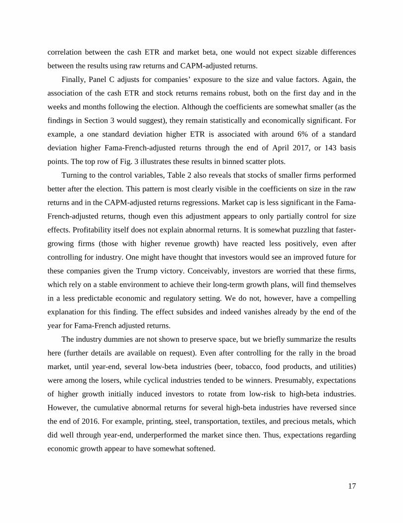
Turning to the control variables, Table 2 also reveals that stocks of smaller firms performed
better after the election. This pattern is most clearly visible in the coefficients on size in the raw
returns and in the CAPM-adjusted returns regressions. Market cap is less significant in the Fama-
French-adjusted returns, though even this adjustment appears to only partially control for size
effects. Profitability itself does not explain abnormal returns. It is somewhat puzzling that faster-
growing firms (those with higher revenue growth) have reacted less positively, even after
controlling for industry. One might have thought that investors would see an improved future for
these companies given the Trump victory. Conceivably, investors are worried that these firms,
which rely on a stable environment to achieve their long-term growth plans, will find themselves
in a less predictable economic and regulatory setting. We do not, however, have a compelling
explanation for this finding. The effect subsides and indeed vanishes already by the end of the
year for Fama-French adjusted returns.
The industry dummies are not shown to preserve space, but we briefly summarize the results
here (further details are available on request). Even after controlling for the rally in the broad
market, until year-end, several low-beta industries (beer, tobacco, food products, and utilities)
were among the losers, while cyclical industries tended to be winners. Presumably, expectations
of higher growth initially induced investors to rotate from low-risk to high-beta industries.
However, the cumulative abnormal returns for several high-beta industries have reversed since
the end of 2016. For example, printing, steel, transportation, textiles, and precious metals, which
did well through year-end, underperformed the market since then. Thus, expectations regarding
economic growth appear to have somewhat softened.
17
Table 2 Cash effective tax rates.
This table presents OLS regressions of individual stock returns on the cash ETR, firm characteristics, and Fama-French 30 industry fixed effects. Panel A uses raw returns, Panel B uses CAPM-adjusted returns, and Panel C uses Fama-French-adjusted returns. The time periods covered are November 9, 2016 (column 1), from November 9, 2016 to December 30, 2016 (column 2), from November 9, 2016 to February 28, 2017 (column 3), and from November 9, 2016 to April 28, 2017 (column 4). The sample includes Russell 3000 firms. T-statistics based on robust standard errors are shown in parentheses. *** p<0.01, ** p<0.05, * p<0.1.
(1) (2) (3) (4)Time period: Nov 9, 2016 Nov 9 - Dec 30 Nov 9 - Feb 28 Nov 9 - April 28Panel A:Cash ETR 0.033*** 0.105*** 0.092*** 0.110***
(3.70) (4.12) (2.83) (2.88)Ln(Market value of equity) -0.551*** -3.246*** -0.961*** -1.347***
Fig. 3. Binned scatter plots of cash ETR (top two panels) and GAAP ETR (bottom two panels) against CAPM-adjusted abnormal returns on November 9, 2016 (left panels) and CARs from November 9 to April 28, 2017 (right panels). The plots control for Fama-French 30 industry fixed effects. The sample includes Russell 3000 firms.
Table 3 and the bottom row of Fig. 3 display the results for the GAAP ETR in place of the
cash ETR. The GAAP ETR reflects the total tax expenses (rather than the cash taxes paid) that a
company records. Again, firms bearing a higher tax burden according to this measure responded
more positively, both for CAPM-adjusted returns and for Fama-French-adjusted returns.
However, as was the case for the cash ETR, and as our discussion at the end of Section 3
portends, the results for Fama-French-adjusted returns are somewhat weaker.
Table 3 suggests that the effect of the GAAP ETR on returns weakens somewhat at the
beginning of 2017 and subsides by the end of April.21 How can this finding be reconciled with
the fact that the effect of the cash ETR remains strong until the end of April? One possible
explanation for the difference between the influence of the cash ETR and the GAAP ETR on
long-run returns is that investors initially considered both ETR measures to be equivalent, but
over time, as they weighed the measures' respective advantages and disadvantages, they
21 As seen in the robustness tests in Section 4.5, when trimming returns, the effect is stronger through the end of April for Fama-French adjusted returns, suggesting that outliers help to account for the insignificant results in Table 3. Moreover, untabulated results show that when adjusting pre-tax income for special items also in the computation of the GAAP ETR (thus using the same denominator as for the cash ETR), the results are stronger and statistically significant for all periods considered.
19
concluded that the cash ETR better proxies future cash tax payments than does the GAAP ETR.
Although this might seem surprising at first sight, since cash taxes can include payments related
to earnings in different tax years, several empirical facts accord with this interpretation. First,
over the period from 1986 to 2016, past cash ETRs predict future cash ETRs better than do past
GAAP ETRs (regressing next year’s cash ETR on the current cash ETR (GAAP ETR) yields R2
values of about 32% (21%)). Second, unlike GAAP ETRs, cash ETRs are unaffected by book
accruals, such as the valuation allowance or the tax contingency reserve (Dyreng, Hanlon, and
Maydew, 2008). Third, there is empirical evidence that firms smooth GAAP ETRs and use the
tax expense to manage earnings (Dhaliwal, Gleason, and Mills, 2004). Future work should
explore in greater depth the long-run relevance of cash and GAAP ETR measures.
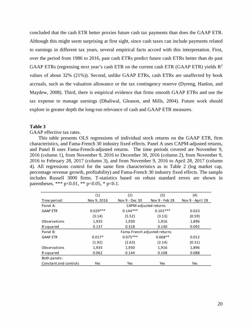
Table 3 GAAP effective tax rates.
This table presents OLS regressions of individual stock returns on the GAAP ETR, firm characteristics, and Fama-French 30 industry fixed effects. Panel A uses CAPM-adjusted returns, and Panel B uses Fama-French-adjusted returns. The time periods covered are November 9, 2016 (column 1), from November 9, 2016 to December 30, 2016 (column 2), from November 9, 2016 to February 28, 2017 (column 3), and from November 9, 2016 to April 28, 2017 (column 4). All regressions control for the same firm characteristics as in Table 2 (log market cap, percentage revenue growth, profitability) and Fama-French 30 industry fixed effects. The sample includes Russell 3000 firms. T-statistics based on robust standard errors are shown in parentheses. *** p<0.01, ** p<0.05, * p<0.1.
(1) (2) (3) (4)Time period: Nov 9, 2016 Nov 9 - Dec 30 Nov 9 - Feb 28 Nov 9 - April 28Panel A:GAAP ETR 0.029*** 0.144*** 0.101*** 0.023
4.2. Deferred tax liabilities and deferred tax assets from net operating loss carryforward
balances
Table 4 examines another set of tax-related consequences. On the one hand, firms with
substantial deferred tax assets (DTAs) arising from net operating loss (NOL) carryforward
balances (henceforth NOL DTAs) should underperform, since a tax cut reduces the present value
of the expected tax savings that these NOLs will provide, which reduces the value of the DTAs.
Note that while the impact of a reduction in the statutory tax rate is clearly negative (in relative
terms) for firms with NOL DTAs, the consequences of the NOL-specific provisions in the House
Republicans’ tax plan tug in both directions: the addition of interest to NOL balances is
beneficial; the introduction of stricter NOL utilization limits hurts. In any event, one would
expect the impact of these additional provisions to be dwarfed by the cut in the statutory rate.
Firms with (net) deferred tax liabilities (DTLs) should benefit: DTLs reflect estimates of
taxes payable in the future should current tax laws remain. If future rates are reduced, the present
value of these liabilities falls, and firm value rises. Table 4 shows that the market reacted in line
with these predicted effects, although the statistical significance of the results for the cash ETR is
weaker than in Table 2, probably because of the smaller number of available observations.
As Panels A and B reveal, the relation between NOL DTAs and abnormal returns is
negative. For CAPM-adjusted returns the effect doesn’t reach statistical significance on the first
day but is strongly significant by year-end. For Fama-French-adjusted returns, the effect is
already significant on the first day. Panels C and D show that (gross) deferred tax liabilities were
significantly positively associated with abnormal returns on November 9. For CAPM-adjusted
returns, the effect remains significant in the November 9 to year-end period and in the period
from November 9 to February 28.
Finally, as Panels E and F show, net DTLs were insignificant on the first day after the
election, but reached significance later on. Presumably, the large number of components in net
DTLs made it harder for market participants to assess their effect on firm value. This is intuitive:
net DTLs are defined as DTLs minus DTAs. While the consequences of a cut in the statutory rate
are relatively easy to assess for DTLs, DTAs include elements that make assessing the effect of a
change in the statutory rate a challenge. (For example, tax credit balances would not be affected,
but a change in the statutory rate would increase the probability that some of the balances cannot
21
be utilized before the expiration of the admissible carryforward period.) Section 5 investigates
differences in the speed of price adjustment among the different variables in detail.
Table 4 Deferred tax liabilities and NOLs.
This table presents OLS regressions of individual stock returns on deferred tax liabilities, NOLs, firm characteristics, and Fama-French 30 industry fixed effects. Panels A and B use deferred tax assets from NOL carryforwards in percent of equity market capitalization (market value of equity, MVE) as the key explanatory variable, Panels C and D use deferred tax liabilities in percent of MVE, and Panels E and F use net deferred tax liabilities in percent of MVE. Panels A, C, and E use CAPM-adjusted returns, while Panels B, D, and F use Fama-French-adjusted returns. The time periods covered are November 9, 2016 (column 1), from November 9, 2016 to December 30, 2016 (column 2), from November 9, 2016 to February 28, 2017 (column 3), and from November 9, 2016 to April 28, 2017 (column 4). All regressions control for the cash ETR and the same firm characteristics as in Table 2. The sample includes Russell 3000 firms. T-statistics based on robust standard errors are shown in parentheses. *** p<0.01, ** p<0.05, * p<0.1.
(1) (2) (3) (4)
Time period: Nov 9, 2016 Nov 9 - Dec 31 Nov 9 - Feb 28 Nov 9 - April 28Panel A:NOL DTA in percent of MVE -0.075 -0.155** -0.089 -0.267*
A number of the policies proposed at one point by President Trump or by Congress would
affect internationally oriented firms differently from domestically focused firms. Some would be
favorable to multinationals, while others would be costly to them, which makes theoretical
predictions on the likely overall impact difficult. This is best illustrated by the discussion around
the taxation of multinationals. Under the current tax regime, firms are taxed on worldwide
income but that tax (with the exception of so-called Subpart F income22) can be deferred until the
foreign subsidiaries remit the monies back to their US parent. When repatriating foreign profits,
firms get a credit for the foreign taxes paid on that income, but typically incur an extra tax cost
because the US corporate tax rate exceeds the tax rate in virtually all countries (so that credits
brought in with the distribution are usually lower than the incremental US tax before credits). A
switch to territorial taxation in accord with the House Republicans’ tax plan (Republicans, 2016)
would benefit multinationals compared to the current system. By contrast, Trump’s tax plan
originally proposed sticking to worldwide taxation albeit ending the deferral of taxes on
22 The Subpart F rules are one of the messiest areas of tax laws and regulations. Under these rules, certain types of income earned by a foreign subsidiary are taxable to the US parent in the year earned even if the foreign corporation does not distribute the income to its shareholder in that year. Broadly speaking, Subpart F income includes investment income such as dividends, interest, rents and royalties; income from the purchase or sale of personal property involving a related person; and income from the performance of services by or on behalf of a related person.
23
corporate income earned abroad (effectively treating all income as Subpart F income), which
would hurt multinationals. This is true ceteris paribus. If the US tax rate were lowered below
foreign rates, repatriation would no longer be associated with an extra tax cost. In his proposal of
April 26, 2017, the President ended up switching to territorial taxation. To the extent that market
participants had viewed this development as likely, foreign-oriented firms should have already
benefited right after the election, or perhaps starting in the weeks and months after the election as
the White House position, though perhaps not widely discussed, started to shift on the matter.
The repatriation of past earnings is another much-discussed policy issue at the intersection
of foreign operations and taxes. Commentators across the political spectrum have worried about
the tendency of US companies to “stash cash abroad”. Such stashing is attractive due to the extra
tax cost firms incur when repatriating foreign subsidiaries’ earnings, as discussed above. If a
partial tax holiday allowed companies to pay a much lower rate when repatriating foreign
earnings, investors might expect companies with cash held abroad to do better. In fact, this
expectation is mirrored in the fact that several years ago, Goldman Sachs compiled a thematic
basket, GSTHSEAS, containing the 50 companies in the S&P 500 with the largest cash positions
held in foreign subsidiaries. Importantly, however, it is not clear how exactly the election would
have affected companies with large unremitted foreign earnings. After all, although it was not
mentioned in her tax plan, a partial tax holiday on repatriated earnings was also widely expected
to occur had Hillary Clinton been elected President. Although Trump advocated a low headline
rate of 10%, he proposed taxing accumulated foreign earnings regardless of whether or not they
are repatriated (through a so-called deemed repatriation).23 Accordingly, the market reaction to
the election on that count would be driven not so much by expectations of a partial tax holiday as
such, but by the perceived difference in the holiday tax rate and the tax base between the two
candidates. Trump was likely to favor a lower rate than would Clinton but to be more aggressive
on the tax base by using the deemed repatriation construct.
A third area where taxes could affect multinationals differently than domestic firms is
through their impact on firms’ competitiveness. The House Republicans’ tax plan (Republicans,
2016) has been interpreted to help make US companies more competitive abroad. The basic
23 A different, but related question is what companies would do with the repatriated cash. Despite explicit prohibitions against the use of repatriated cash for repurchases, it appears that this is exactly what companies did use this cash for after the 2004 tax holiday (Dharmapala, Foley, and Forbes, 2011). Thus, an indirect effect leading to differential stock market reactions to repatriation could be due to differences in firms’ financial constraints.
24
thrust of the plan is that US companies would not pay tax on profits earned on overseas sales
anymore. Conversely, products, services and intangibles that are imported would be subject to
US tax regardless of where they are produced (“border adjustment”). [See Tax Foundation
(2016) for a description of the plan.] The Tax Foundation, however, dismisses the argument that
exporters would benefit from the plan. They write: “Of course, U.S. producers may think of this
as a subsidy for exports because they would not be taxed on sales overseas. But if businesses
were able to reduce the prices of their goods they sell overseas due to the border adjustment, this
would trigger a higher demand for dollars in order to purchase those goods. This higher demand
for dollars would increase the value of the dollar relative to foreign currencies and offset any
perceived trade advantage granted by the border adjustment.” Following this view, some market
observers have claimed that (expectations of) the plan’s enactment would lead to a substantial
appreciation of the dollar (which has, however, not happened during the period). President
Trump never endorsed the border adjustment idea, and it was not part of the proposal presented
by Secretary Mnuchin on April 26, 2017.
Finally, several factors not directly related to taxes might favor domestically focused stocks.
First, market participants may have higher expectations for US growth versus foreign growth.
Second, firms active abroad are more subject to the risk of trade retaliation from other countries.
In either case, firms with larger foreign presence would suffer. (Without further evidence, one
cannot distinguish between the two explanations, although the fact that many foreign stock
markets have performed as well as US markets since the election casts doubt on the theory that
differences in growth expectations favor more domestically oriented US firms.24) Third, Trump’s
proposed infrastructure plans would naturally benefit domestically focused firms. Fourth,
Trump’s expansionist fiscal intentions and the associated increase in inflation expectations are
likely to foster Fed rate hikes. In a number of speeches following the election, Federal Reserve
officials suggested that they might tighten policy faster if fiscal policy became more
expansionary.25 While higher inflation per se would hurt the dollar in the long run, the rate hikes
24 Between November 8, 2016 and April 28, 2017, the MSCI World ex USA total return (TR) index rose by 11.60%, the Stoxx Europe 600 TR index by 17.05%, the Nikkei 225 TR index by 12.82%, and the Russell 3000 TR index by 13.08%. 25 The minutes of the December 2016 FOMC meeting, which were released on January 4, 2017, for example, are in line with these statements made by Fed officials before year-end. The minutes state: “Many participants noted that there was currently substantial uncertainty about the size, composition, and timing of prospective fiscal policy changes, but they also commented that a more expansionary fiscal policy might raise aggregate demand above sustainable levels, potentially necessitating somewhat tighter monetary policy than currently anticipated.”
25
could initially strengthen it, hurting exporters.26 According to the minutes of the December 2016
FOMC meeting, “[s]urveys of market participants had indicated that revised expectations for
government spending and tax policy following the U.S. elections in early November were seen as
the most important reasons, among several factors, for the increase in longer-term Treasury
yields, the climb in equity valuations, and the rise in the dollar.”
Summarizing, policies that Trump has trumpeted could both hurt and help exporters and
firms with significant foreign operations, and it is not obvious whether hurt or help would
predominate.27 But investors through the stock market did take a view. Panels A and B of Table
5 and Fig. 4 suggest that investors strongly believed that domestically oriented companies would
be relatively advantaged: abnormal returns are significantly negatively related to the fraction of
revenues being earned outside the US. Interestingly, the negative relation between foreign
revenue and stock returns was strong not only on the day following the election, but persisted
and strengthened in the following days and weeks. Again, Section 5 will elaborate on the speed
of price adjustment. Table 5 also shows that from year-end through the end of April,
internationally oriented companies appear to have done somewhat better (though the difference
is not significant at conventional levels). This finding is consistent with, among other things, the
border adjustment tax becoming less and territorial taxation becoming more likely over time than
they seemed just after the election, or with the prospects for trade war diminishing. However, the
net effect, by the end of April, still was that domestically oriented companies had a strongly
significant advantage.
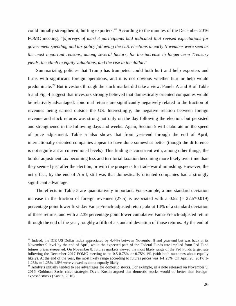
The effects in Table 5 are quantitatively important. For example, a one standard deviation
increase in the fraction of foreign revenues (27.5) is associated with a 0.52 (= 27.5*0.019)
percentage point lower first-day Fama-French-adjusted return, about 14% of a standard deviation
of these returns, and with a 2.39 percentage point lower cumulative Fama-French-adjusted return
through the end of the year, roughly a fifth of a standard deviation of those returns. By the end of
26 Indeed, the ICE US Dollar index appreciated by 4.44% between November 8 and year-end but was back at its November 9 level by the end of April, while the expected path of the Federal Funds rate implied from Fed Fund futures prices steepened. On November 8, futures markets viewed the most likely range of the Fed Funds target rate following the December 2017 FOMC meeting to be 0.5-0.75% or 0.75%-1% (with both outcomes about equally likely). At the end of the year, the most likely range according to futures prices was 1-1.25%. On April 28, 2017, 1-1.25% or 1.25%-1.5% were viewed as about equally likely. 27 Analysts initially tended to see advantages for domestic stocks. For example, in a note released on November 9, 2016, Goldman Sachs chief strategist David Kostin argued that domestic stocks would do better than foreign-exposed stocks (Kostin, 2016).
26
April, the effect had about halved, though it remained sizable, with a company with a one
standard deviation higher fraction of foreign revenues having experienced a 1.46 percentage
point lower cumulative return.
-4-3
-2-1
01
23
45
AR
on
Nov
9
0 20 40 60 80 100Percent foreign revenues
-4-3
-2-1
01
23
45
CA
R N
ov 9
to A
pril
28
0 20 40 60 80 100Percent foreign revenues
Fig. 4. Binned scatter plots of percent revenue from foreign sources against CAPM-adjusted abnormal returns on November 9, 2016 (left panel) and CARs from November 9 to April 28, 2017 (right panel). The plots control for Fama-French 30 industry fixed effects and the cash ETR. The sample includes Russell 3000 firms.
The remaining panels report similar results for other measures of foreign operations. The
share of profits due to foreign operations (Panels C and D) and the degree of foreign activity
(Panels E and F) are both negatively related to firms’ stock market performance, both
immediately after the election and through year-end. However, results available on request show
that they are significantly positively related to cumulative returns from January 3 (the year’s first
trading day) to April 28, consistent with the result seen for foreign revenues.
Some observers argued that the administration’s tax plan would hurt importers. On the other
hand, while foreign assets arguably proxy well for foreign production costs, such foreign
production might not lead to imports, and conversely companies may import significant amounts
of goods without owning production assets abroad. Overall, the fraction of non-US assets is
significantly negatively related to stock returns, though this was not reflected in the first-day
reaction; see Panels G and H. Here, the drift continued beyond year-end, indeed at least through
the end of April. We caution that the sample is relatively small for this last analysis.
27
Table 5 Foreign operations.
This table presents OLS regressions of individual stock returns on measures of foreign operations, firm characteristics, and Fama-French 30 industry fixed effects. Panels A, C, E, G, and I use CAPM-adjusted returns, Panels B, D, F, H, and J use Fama-French-adjusted returns. The time periods covered are November 9, 2016 (column 1), from November 9, 2016 to December 30, 2016 (column 2), from November 9, 2016 to February 28, 2017 (column 3), and from November 9, 2016 to April 28, 2017 (column 4). All regressions control for the cash ETR and the same firm characteristics as in Table 2. The sample includes Russell 3000 firms. T-statistics based on robust standard errors are shown in parentheses. *** p<0.01, ** p<0.05, * p<0.1.
(1) (2) (3) (4)Time period: Nov 9, 2016 Nov 9 - Dec 31 Nov 9 - Feb 28 Nov 9 - April 28Panel A:Percent revenue from foreign sources -0.014*** -0.069*** -0.065*** -0.048**
Let us turn to the issue of the repatriation of past earnings. Panels I and J of Table 5 reveal
that companies holding large amounts of cash in foreign subsidiaries in fact responded worse to
the Trump election. After controlling for foreign revenues (not shown), however, the effect turns
insignificant, suggesting that foreign cash holdings at least partly proxy for a firm’s overall
foreign activities.
It is difficult to parse among the possible explanations for the underperformance of
internationally oriented firms: fears of retaliatory tariffs or trade wars, expectations of the end of
the deferral of foreign source income, and concerns about the taxation of accumulated foreign
earnings. What is striking is that underperformance is found based on most of the measures of
foreign orientation that we consider.
29
4.4. Capital investment expensing and interest expense deductibility
Another tax-related proposal for making the US more competitive is to strengthen firms’
incentives to invest. Specifically, under the House Republicans’ tax plan, businesses would no
longer need to depreciate capital investments. Rather, they would be able to expense them fully
in the period that they are made. Thus, firms would be able to defer corporate income taxes,
which should lift their stock prices, with larger effects for firms making greater capital
expenditures relative to their size. To avoid a tax subsidy for debt-financed investment, the
House Republicans’ plan would no longer allow net interest expenses to be deducted. This would
hurt those firms with greater leverage (which generates value through the tax shield in place up
to now) and those with greater proportional interest expenses.
As expected, firms with substantial interest expenses reacted more negatively, as seen in
Panels A and B of Table 6. This result may not reflect any expectation regarding interest
deductibility being abolished; deductions also lose value when taxes are slashed. However, note
that we control for profitability, so at least part of the direct tax effect should be accounted for.
Panels C and D also reveal a negative relation between firm leverage and abnormal returns.
In results not presented, we find no significant relation between immediate or long-run
abnormal returns and CAPEX. (These regressions control for leverage and interest expenses. The
lack of such results is not surprising, as any benefit from immediate expensing would be offset to
some extent by the non-deductibility of interest, assuming the investments would have been
financed with bonds. The same results hold when not controlling for these variables.) Thus,
investors seemed to believe that either the Republicans’ proposed capital expenditure rule is
unlikely to have large effects, or that it is unlikely to be implemented.28
28 While the House Republicans’ plan removes interest deductibility for all firms and allows all firms to expense capital investments, Trump’s campaign plan (Trump, 2016) was to restrict the possibility to expense capital investment to manufacturers. These companies would be allowed to opt (once in three years) to expense, but would then give up the interest deduction. When confining the sample to the 583 firms with complete data in SIC codes 2000 to 3999 (manufacturing), the coefficient on capital expenditures varies in sign and is mostly insignificant in regressions like those in Table 6.
30
Table 6 Interest expense deductibility and leverage.
This table presents OLS regressions of individual stock returns on interest expenses, leverage, firm characteristics, and Fama-French 30 industry fixed effects. Panels A and C use CAPM-adjusted returns, Panels B and D Fama-French-adjusted returns. The time periods covered are November 9, 2016 (column 1), from November 9, 2016 to December 30, 2016 (column 2), from November 9, 2016 to February 28, 2017 (column 3), and from November 9, 2016 to April 28, 2017 (column 4). All regressions control for the cash ETR, foreign revenue, and the same firm characteristics as in Table 2. The sample includes Russell 3000 firms. T-statistics based on robust standard errors are shown in parentheses. *** p<0.01, ** p<0.05, * p<0.1.
(1) (2) (3) (4)Time period: Nov 9, 2016 Nov 9 - Dec 31 Nov 9 - Feb 28 Nov 9 - April 28Panel A:Interest expense in percent of assets -0.210** -1.043*** -0.468 -0.986*
This table presents OLS regressions of winsorized or trimmed individual stock returns on firm characteristics and Fama-French 30 industry fixed effects. The specifications used to investigate the impact of the different explanatory variables match those in Tables 2 – 6. Specifically, Panel A (cash ETR) uses the specification from Table 2, Panel B (GAAP ETR) that from Table 3, Panels C and D (NOL DTAs and DTLs) the specifications from Panels A to D in Table 4, Panels E and F (foreign revenue and profits) the specifications from Panels A to D in Table 5, and Panel G (interest expense) the specifications from Panels A and B in Table 6. Columns (1) to (4) show results when abnormal returns are winsorized at the 1% and 99% levels, and Columns (5) to (8) trim the observations with the 1% highest and lowest returns. Results are presented for both CAPM-adjusted returns (columns (1)-(2) and (5)-(6)) and Fama-French-adjusted returns (columns (3)-(4) and (7)-(8)). The time periods covered are November 9, 2016 (odd columns) and from November 9, 2016 to April 28, 2017 (even columns). The sample includes Russell 3000 firms. T-statistics based on robust standard errors are shown in parentheses. *** p<0.01, ** p<0.05, * p<0.1.
A potential concern regarding the analysis above is that extreme returns might confound our
inferences. We now briefly present summary results for our key findings when adjusting outlier
returns. Columns (1) to (4) of Table 7 show results when abnormal returns are winsorized at the
1% and 99% levels, and Columns (5) to (8) trim the observations with the 1% highest and lowest
returns. The specifications used to investigate the impact of the different explanatory variables
match those in Tables 2 to 6. Virtually the same findings emerge as before, though often with
higher statistical significance.
5. The speed of information processing: A price contribution analysis Section 4 reveals that firms’ effective tax rates, deferred tax assets from net operating loss
carryforwards, gross and net deferred tax liabilities, foreign operations, leverage, and interest
expenses each sizably impacted stock returns after the election. Furthermore, the market
responded immediately, with all but one variable starting to affect stock returns on the day
following the election. However, the results in Section 4 also show that for almost all variables,
the long-term response exceeded the short-term one, suggesting that markets needed some time
to digest information. This section examines the differential speeds with which the different
variables were incorporated into the cross-section of stock returns.
Although all variables are public information, such differential speeds would not be
surprising for several reasons. First, while some variables are included in firms’ financial
statements, others (such as information on foreign revenues) are sometimes harder to obtain.
Second, knowing the realization of a given variable for a particular firm is not enough: the likely
impact of policy changes on that firm’s prospects must then be assessed, and the complexity of
doing so differs across variables. For example, assessing the effect of gross deferred tax
liabilities appears relatively straightforward, since such liabilities reflect existing transactions
and already account for timing differences between financial and tax accounting. By contrast,
assessing the effect of net deferred tax liabilities would require further calculation: as mentioned
above, deferred tax assets include tax credits for which the effect of a change in the statutory rate
is less than obvious. Assessing the impact of foreign revenue on a particular firm is also quite
involved, particularly given that it is likely to reflect a combination of tax- and trade-related
effects, each of which is quite challenging to assess. For example, quantifying the impact of a
33
switch to territorial taxation or an end to the deferral of foreign taxes would require information
on a firm’s effective foreign tax rate in the different foreign tax credit limitation baskets.29
Similarly, the likelihood of both US trade restrictions and retaliation differs across countries, but
few firms provide a breakdown of foreign revenue by country.
To assess the speed at which the information from the different variables was incorporated
into prices, we adapt the price contribution (PC) methodology commonly used in the market
microstructure literature to our setting (see, e.g., Barclay and Hendershott, 2003). The goal is to
measure the fraction of the price impact of variable i on abnormal stock returns that have accrued
up to day t.
To simplify the exposition, we first discuss the analysis for market returns and then describe
its extension to our explanatory variables. For each trading day t, the cumulative price
contribution measure for the market return, MTtPC , , is simply the fraction of the cumulative
market return (up to a given end point T) that has accrued by the close of that trading day, i.e.,
T
tMTt R
RPC
,0
,0, = , (4)
where tR ,0 denotes the cumulative return from the election to trading day t.
Our innovation obtains a similar measure for our cross-sectional explanatory variables. To
secure it, on each trading day t we estimate the regression coefficients corresponding to each
variable i using cumulative stock and market returns from the election up to that day, it,0β . We
then compute the cumulative price contribution measure for each variable i, iTtPC , , using the
regression betas instead of returns, i.e.,
iT
iti
TtPC,0
,0, β
β= . (5)
By construction, 0,0 =iTPC and 1, =i
TTPC for all i, and iTtPC , provides a measure over time of
the share of the overall price move in the cross-section of stock returns associated with variable i
that has taken place by day t.
29 Separate limitations on foreign tax credit utilization apply to different categories of income, the main ones being general limitation income and passive income.
34
A similar analysis can be performed for variance to assess the timing of resolution of price
uncertainty related to each of the variables. The variance contribution for each trading day is the
square of the difference in the change in the cumulative market return or beta compared to the
previous trading day divided by the sum of such squares across all trading days. The cumulative
variance contribution is then computed as the sum of the daily variance contributions up to that
day. Formally, the cumulative variance contribution for the market return for day t, MTtVC , , is
given by
∑∑
= −
= −
−
−= T
s ss
t
s ssMTt
RR
RRVC
12
1,0,0
12
1,0,0,
)(
)(, (6)
where we use the convention that R0,0 = 0. Replacing R with βi yields the corresponding
expression for variable i, iTtVC , . Here, too, by construction, 0,0 =i
TVC and 1, =iTTVC for all i.
Before we present the results, it is useful to illustrate the difference between the two
measures. If the one-day response of two variables equals their T-day response but the first
settles after the first day and the second keeps moving around for several days, the price
contribution on the first day will be one for both variables, but variance contribution for the first
variable will exceed that for the second.
Fig. 5 shows how the CAPM-adjusted abnormal returns associated with each of the
variables in Section 4 and the market return accrued during the first ten trading days after the
election.30 All results are based on the specifications used in Tables 2 to 6. The upper panel
reports the cumulative price contributions, and the lower panel the cumulative variance
contributions. We differentiate between the first day and the following days.
Consider the upper panel first. As the figure shows, speeds of price adjustment differ
considerably across variables. Deferred tax liabilities (labeled “DTL / MVE” in the figure) and
deferred tax assets from NOL carryforwards (NOL DTAs) had the strongest first-day impact. For
example, the value of about 0.8 for deferred tax liabilities says that 80% of the impact of
deferred tax liabilities on returns that arose during the first ten trading days after the election was
already reflected in prices on the first day. ETRs, leverage, interest expense, and foreign
30 Of course, ten trading days is somewhat arbitrary. It is apparent from Fig. 1 that some information was processed during the first weekend, maybe because investors had some time to reflect on the implications of the election. Adding another week seems sensible. We thus round up to 10 days. Considering eight (i.e. up to Friday, November 18) or 12 trading days (i.e. up to Friday, November 25 since November 24 was the Thanksgiving holiday) yields similar patterns.
35
exposure were priced in modestly on the first day, all achieving less than 30% of their ten-day
effect. Starting on the second day, however, investors began to strongly impound these
characteristics into prices, quickly overtaking the extent to which NOL DTAs were priced. Net
DTLs were priced in the most slowly; they had virtually no impact on prices on the first day.
Thus, consistent with most of the literature on price responses, we find evidence public
information is incorporated into prices with a delay.
As prices respond to major information shocks along multiple dimensions, we should expect
some variables to overshoot. That is precisely what happened with deferred tax liabilities, the
variable that had the strongest relative first-day impact. By the second day it had overshot and by
the fourth it was 50% over; hence, it eventually reversed. Interestingly, the first-day move
associated with DTLs, and NOL DTAs also, was stronger than that in the overall market, while
from the second day onwards, the price contribution for most variables exceeded that of the
market.
The cumulative variance contributions in the bottom panel reveal a picture similar to that of
the price contributions. About 60% (over 70%) of the variability in the deferred tax liability
(NOL DTA) coefficient that took place during the first ten trading days occurred on the first day,
while none of the variability associated with net DTLs took place on the first trading day. The
market return showed an intermediate outcome, with roughly half of the variability occurring on
the first trading day. The cash ETR, GAAP ETR, and foreign revenue initially affected prices at
similar speeds, with 20% to 30% of the ten-day variability taking place on the first day. Looking
beyond the first day, most of the variability in the effect of both ETRs, gross DTLs, NOL DTAs,
leverage, and interest expense had essentially taken place by the second day, with the variance
contribution of all these variables reaching about 80% or more. By contrast, foreign revenue took
until the fourth day and net DTLs until the seventh day to get 80% reflected in prices.
Fig. 6 shows the results of similar computations when using Fama-French-adjusted returns
rather than CAPM-adjusted returns; the results are remarkably similar. The one notable
difference is that the impact of NOL DTAs on prices on the first day after the election is
somewhat smaller than for CAPM-adjusted returns.
In sum, the findings in this section reveal that from the first day market prices moved in the
appropriate, i.e., ten-day direction. (Net DTLs were a mild exception; they did not move on the
first day.) However, the market under-responded, since all movements from day one to day ten
36
(again with the exception of net DTLs) albeit in the same direction as the first-day moves, were
considerably greater. All eight variables are public information, yet they affected prices at
notably different speeds.
Fig. 5. Cumulative price and variance contribution using CAPM-adjusted returns. This figure shows the cumulative price (upper panel) and variance (lower panel) contributions of the different explanatory variables and of the market return during each of the ten trading days following the election. For the market return, the cumulative price contribution measures the fraction of the cumulative market return (up to a given end point T, here ten trading days) that has accrued by the close of day t. The cumulative price contribution for the different cross-sectional explanatory variables (the cash ETR, GAAP ETR, etc.) measures the share of the overall price move in the cross-section of stock returns associated with that variable that has taken place by day t. The cumulative variance contribution measures the share of the price uncertainty related to each of the variables that is resolved by day t. The sample includes Russell 3000 firms, and the computations are based on CAPM-adjusted returns.
37
Fig. 6. Cumulative price and variance contribution using Fama-French-adjusted returns. This figure shows the cumulative price (upper panel) and variance (lower panel) contributions of the different explanatory variables and of the market return during the ten trading days following the election. The computation of both measures is described in Fig. 5. The sample includes Russell 3000 firms, and the computations are based on Fama-French-adjusted returns.
6. Trump troubles and stock price movements: An out-of-sample test Events beyond its first hundred days have brought new troubles for the Trump Presidency.
The market in aggregate at least initially responded quite negatively to the news cycle
surrounding the firing of FBI Director Comey. On May 9, 2017, after the market close, news
broke that President Trump had fired Director Comey. While the official statement at first
indicated that he had been fired for mishandling the Hillary Clinton email probe, media outlets
quickly connected the firing to the fact that Mr. Comey had been supervising the investigation
into possible connections between the Trump campaign and Russia. On the following day, in a
meeting with Russian foreign minister Lavrov and Russian ambassador Kislyak, Trump said “I
38
just fired the head of the FBI” and added, referring to Comey: “He was crazy, a real nut job. I
faced great pressure because of Russia. That's taken off.” On May 16 (again after the market
close), news surfaced about the existence of a memo written by Comey following his meeting
with Trump on February 14. That memo stated that President Trump had tried to convince
Comey to drop the investigation against his former National Security advisor Flynn, saying, “I
hope you can let this go.” Some media accounts suggested that this represented obstruction of
justice, a serious offence. Stock index futures started dropping during overnight trading. On May
17, stock markets plunged, with the Russell 3000 falling 1.86%, its biggest drop in eight months.
On the evening of May 17, former FBI Director Robert Mueller was appointed as a special
counsel to oversee the Russia probe.
While far from being as consequential or surprising as the original event, the election, it is
worth exploiting this “beyond-study-period” event to test our conjecture that taxes matter greatly
to firm value. The market viewed the President as having gotten into trouble. Therefore, the
probability of tax reform being delayed, being smaller, or simply being shelved had increased.
Indeed, political betting markets showed that the probability of Trump’s impeachment or leaving
office before the end of his term had risen sharply and the probability of a corporate tax cut had
fallen substantially in this period.31 Reduced prospects for tax reform should be relatively bad
news for high-tax firms. Table 8 provides some support for this idea.
On May 10 (the first trading day after the Comey firing), high-tax firms reacted modestly
negatively (but not significantly so). On May 17 (the day of the big negative aggregate move),
high-tax firms lost significantly. Internationally oriented firms also lost on that day. This is
consistent with the fact that since the end of the year, these companies had actually been doing
relatively well, as mentioned in Section 4.3. Once again, this effect may be due to a combination
of factors, ranging from mere ripples (tax reform being delayed) to earthquakes (Trump losing
the Presidency).
31 For example, on PredictIt.org, the probability of Trump still being president at the end of 2018 dropped from 74% on May 8 to 56% on May 17, while Ladbrokes (2017) reports that Trump was, on May 17, odds-on to be impeached. Over the same period, the probability of the corporate tax rate being cut by the end of 2017 on PredictIt.org dropped from 58% to 36%.
39
Table 8 Trump Troubles.
This table presents OLS regressions of individual stock returns on firm characteristics and Fama-French 30 industry fixed effects. Panels A and C use CAPM-adjusted returns, Panels B and D Fama-French-adjusted returns. The event dates are May 10, 2017 (column 1) and May 17, 2017 (column 2). Panels A and B include the cash ETR. Panels C and D include, in addition, percent foreign revenue. All regressions include the standard controls (log market cap, revenue growth, profitability, and Fama-French 30 industry fixed effects). The sample includes Russell 3000 firms. T-statistics based on robust standard errors are shown in parentheses. *** p<0.01, ** p<0.05, * p<0.1.
(1) (2)
Days: May 10, 2017 May 17, 2017Panel A:Cash ETR -0.007 -0.017***
7. Conclusion The election of Donald J. Trump as the 45th President of the United States of America
surprised the nation and its investors. Expectations for significant tax reductions skyrocketed
given that Republicans would also control both houses of Congress. This study traces stock
market reactions from the day before the election through President Trump’s first hundred days
in office. It finds strong evidence that the cross-section of stock returns over this period reflects
40
expectations of a major corporate tax cut. Specifically, high tax-paying firms (as measured by
both the cash ETR and the GAAP ETR) and those with high deferred tax liabilities benefitted
substantially, while those with large deferred tax assets from NOL carryforwards
underperformed. Investors also downgraded companies with high leverage and high interest
expenses, due to the loss of deductibility under some prominent tax reform plans. By contrast,
investors think that plans to allow immediate expensing of capital investments are either unlikely
to be implemented, or of little consequence.
Stock prices show that investors are concerned about US companies with significant foreign
exposure. There are many possible explanations of internationally oriented firms’
underperformance: fears of retaliatory tariffs or trade wars, expectations of the end of the tax
deferral of foreign source income, and concerns about the taxation of accumulated foreign
earnings. Each by itself could contribute to the underperformance finding.
It is worth stressing that these significant relative stock movements have been
overwhelmingly due to changes in expectations about policies, not policy changes themselves,
since by the one-hundred-day mark no legislation had even been initiated on either tax policy or
fundamental foreign trade matters. Interestingly, markets digested information in the above-
mentioned factors influencing the differential performance of stocks at varying speeds. To
examine the important question of how quickly different types of information gets incorporated
into stock prices, we adapt the price contribution methodology commonly used in the
microstructure literature to our multidimensional setting. Specifically, rather than considering
returns on individual assets, we use the cross-section of stock price reactions over the ten days
after the election to assess the speed of price adjustment for each factor. To our knowledge, this
is the first time that coefficients from a cross-section of stock price reactions have been used to
measure the speed of information processing. We believe that this method can be fruitfully
employed in a range of other settings.
Specifically, we examine the major movements in stock prices in the first ten days after the
election, and determine how much of the movement due to the above factors had occurred by
each day. None of the eight factors exerted its full effect the first day; indeed all but one crept up
through the first three days. Deferred tax liabilities experienced the fastest impact, 80% of its
total on the first day. Next fastest were deferred tax assets from NOL carryforwards. As might be
expected, net deferred tax liabilities (whose effect is cumbersome to assess for reasons that we
41
discuss in the paper) were slowest. The positive impact of expected policy changes on firms with
high cash and GAAP ETRs, and their negative impact on high-leverage firms, firms with large
interest expenses, and internationally-oriented firms required several days to be reflected in
prices. Their one-day response equaled only about 30% of their ten-day response.
The Trump election and the early days of the Administration affected the relative health of
corporations, as reflected in their stock market reactions. This dramatic change in circumstances
is likely to spur additional work in the future study of empirical corporate finance topics. First,
there are surely additional dimensions that one can look at in the cross-section of stock returns.32
Second, company policy responses may also be observed, especially as regards investments and
perhaps even capital structure decisions. The choice to take losses (perhaps even “big baths”) can
also be a function of expected tax changes. For example, Warren Buffett indicated at Berkshire
Hathaway’s 2017 shareholder meeting that because realizing losses would offset Berkshire’s
other profits, this option would be more valuable while taxes remain high. As of the time of this
writing, whether the potential corporate tax reform envisioned by the current Administration will
be realized, and if so how adjusted, is unclear. Yet, as Hanlon and Hoopes (2014) point out (p.
123), in other cases, firms have responded to proposed changes to (dividend) tax law that
eventually did not materialize.
Substantial new information will unfold as the Trump Presidency progresses, particularly
since so few policies were actually implemented in the first hundred days. Expectations drove
price movements from the election to the hundred-day point. Expectations about policies may
not be realized. If not, relative prices can be expected to revert. The events of May, analyzed
above, provide a striking example of such a reversal. Trump's troubles, including the Russia
investigation, the failure to advance his agenda on health care reform, and the upheaval in the
White House staff, continued into the summer of 2017. If the market thought that these troubles
significantly dampened prospects for a sizable corporate tax cut, then the substantial
outperformance of high-tax firms since Election Day should decline. Whatever one’s politics, the
first period of the Trump Presidency lends confidence to one prediction: significant policy
surprises, and significant changes in company stock prices, lurk in the near- and not-so-near term
future.
32 For example, in a more recent study, Brown and Huang (2017) investigate how immediate stock price reactions to the 2016 election vary depending on executives’ access to President Obama.
42
References
Amromin, G., Harrison, P., Sharpe, S., 2008. How did the 2003 dividend tax cut affect stock prices? Financial Management 37, 625-646.
Auerbach, A.J., Hassett, K.A., 2006. Dividend taxes and firm valuation: new evidence. American Economic Review 96, 119-123.
Auerbach, A.J., Hassett, K.A., 2007. The 2003 dividend tax cut and the value of the firm: an event study. In: Auerbach, A.J., Hines, J., Slemrod, J. (Eds.) Taxing Corporate Income in the 21st Century. Cambridge University Press, New York, NY, pp. 93-126.
Barclay, M.J., Hendershott, T., 2003. Price discovery and trading after hours. Review of Financial Studies 16, 1041-1073.
Brown, J.R., Huang, J., 2017. All the President's friends: political access and firm value. Unpublished working paper. University of Illinois at Urbana-Champaign.
Dhaliwal, D.S., Gleason, C.A., Mills, L.F., 2004. Last-chance earnings management: using the tax expense to meet analysts' forecasts. Contemporary Accounting Research 21, 431-459.
Dharmapala, D., Foley, C.F., Forbes, K.J., 2011. Watch what I do, not what I say: the unintended consequences of the Homeland Investment Act. The Journal of Finance 66, 753-787.
Dyreng, S.D., Hanlon, M., Maydew, E.L., 2008. Long-run corporate tax avoidance. The Accounting Review 83, 61-82.
Dyreng, S.D., Hanlon, M., Maydew, E.L., Thornock, J.R., 2017. Changes in corporate effective tax rates over the past 25 years. Journal of Financial Economics Forthcoming
Graham, J., 2003. Taxes and corporate finance: a review. Review of Financial Studies 16, 1075-1129.
Graham, J., Hanlon, M., Shevlin, T., 2011. Real effects of accounting rules: evidence from multinational firms’ investment location and profit repatriation decisions. Journal of Accounting Research 49, 137-185.
Hanlon, M., Heitzman, S., 2010. A review of tax research. Journal of Accounting and Economics 50, 127-178.
Hanlon, M., Hoopes, J.L., 2014. What do firms do when dividend tax rates change? An examination of alternative payout responses. Journal of Financial Economics 114, 105-124.
Knight, B., 2007. Are policy platforms capitalized into equity prices? Evidence from the Bush/Gore 2000 Presidential Election. Journal of Public Economics 91, 389-409.
Kostin, D., 2016. US equity implications of a Trump Presidency. Goldman Sachs, downloadable at: http://www.zerohedge.com/news/2016-11-09/revisionism-arrives-goldman-says-trumps-victory-will-have-little-impact-market
Ladbrokes, 2017. Donald Trump now just 4/5 to be impeached in first term (May 17, 2017). URL http://news.ladbrokes.com/politics/american-politics/donald-trump-now-just-45-to-be-impeached-in-first-term.html
Mills, L.F., Newberry, K.J., Novack, G.F., 2003. How well do Compustat NOL data identify firms with U.S. tax return loss carryovers? Journal of the American Taxation Association 25, 1-17.
Niederhoffer, V., Gibbs, S., Bullock, J., 1970. Presidential elections and the stock market. Financial Analysts Journal 26, 111-113.
Republicans, 2016. A Better Way -- Tax Policy Paper (June 24, 2016). House Republicans, Washington, DC.
Santa-Clara, P., Valkanov, R., 2003. The Presidential puzzle: political cycles and the stock market. The Journal of Finance 58, 1841-1872.
Wolfers, J., Zitzewitz, E., 2016. What do financial markets think of the 2016 election? Unpublished working paper. University of Michigan and Dartmouth College.