+ All Categories
Home > Documents > TTA Report 1 - NRAO Library · • ETP — Energetic Transients and Pulsars; ... • ISM —...

TTA Report 1 - NRAO Library · • ETP — Energetic Transients and Pulsars; ... • ISM —...

Date post: 18-Apr-2018
Category:
Upload: vuongmien
View: 217 times
Download: 2 times
Share this document with a friend
80
COMMENTS ON PEER REVIEW AND RATING OF NRAO OBSERVING PROPOSALS Frederic R. Schwab, Dana S. Balser, and Gareth C. Hunt March 10, 2015 1. Introduction Recently we were asked to comment on the NRAO proposal peer review process, and to focus primarily on the scoring procedure reviewers are instructed to follow and the algorithm used for aggregation of the reviewers’ scores. In particular, we were asked to comment on the robustness of the score aggregation process—for example, sensitivity to imbalance between reviewers’ score distributions—and to compare our proposal scoring system with those used by other institutions and other observatories (e.g., ESO, Arecibo, HST, etc.) in order to provide assurance that our practice is not out of the mainstream. We begin by summarizing, in Section 2, the mechanics of the current review process for standard GBT, VLA, and VLBA proposals. There we describe the instructions provided to reviewers for scoring, the score normalization and averaging method that is used, and the peculiarities (particular the imbalance) of the distributions of reviewers’ observed raw score distributions for recent proposal review cycles. We continue with a discussion of possible deficiencies in our proposal scoring system and suggest a few simple remedies. In Section 3 we compare the NRAO process with what is in use at other observatories and at two federal agencies, NSF, and NIH. In Section 4 we discuss ranking, rating, and score aggregation methods that are based on pairwise score comparisons. In Section 5, we discuss two other methods that have appeared in recent literature, and in Section 6 we call attention to a recent paper advocating a distributed approach to telescope proposal peer review. Conclusions are given in Section 7, along with a few more comments and suggestions. 2. Description of the Review Process The NRAO Web pages give a useful overview of the review process, one intended both for reviewers and proposers. 1 Also, a comprehensive description of the gritty, technical details of the process is given in a memorandum by Bryan Butler [1], titled “Requirements for the PST for the New NRAO Proposal Evaluation and Time Allocation Process”, dated October 13, 2010. We include that memorandum here as Appendix A. Most of the details there are still current. This process pertains to proposals for use of North American NRAO facilities—the GBT, VLA, and VLBA. 1 See https://science.nrao.edu/observing/proposal-types . 1 TTA Report 1
Transcript

COMMENTS ON PEER REVIEW AND

RATING OF NRAO OBSERVING PROPOSALS

Frederic R. Schwab, Dana S. Balser, and Gareth C. Hunt

March 10, 2015

1. Introduction

Recently we were asked to comment on the NRAO proposal peer review process, and tofocus primarily on the scoring procedure reviewers are instructed to follow and the algorithmused for aggregation of the reviewers’ scores. In particular, we were asked to comment on therobustness of the score aggregation process—for example, sensitivity to imbalance betweenreviewers’ score distributions—and to compare our proposal scoring system with those usedby other institutions and other observatories (e.g., ESO, Arecibo, HST, etc.) in order toprovide assurance that our practice is not out of the mainstream.

We begin by summarizing, in Section 2, the mechanics of the current review process forstandard GBT, VLA, and VLBA proposals. There we describe the instructions provided toreviewers for scoring, the score normalization and averaging method that is used, and thepeculiarities (particular the imbalance) of the distributions of reviewers’ observed raw scoredistributions for recent proposal review cycles. We continue with a discussion of possibledeficiencies in our proposal scoring system and suggest a few simple remedies. In Section 3we compare the NRAO process with what is in use at other observatories and at two federalagencies, NSF, and NIH.

In Section 4 we discuss ranking, rating, and score aggregation methods that are based onpairwise score comparisons. In Section 5, we discuss two other methods that have appearedin recent literature, and in Section 6 we call attention to a recent paper advocating adistributed approach to telescope proposal peer review.

Conclusions are given in Section 7, along with a few more comments and suggestions.

2. Description of the Review Process

The NRAO Web pages give a useful overview of the review process, one intended bothfor reviewers and proposers.1

Also, a comprehensive description of the gritty, technical details of the process is givenin a memorandum by Bryan Butler [1], titled “Requirements for the PST for the NewNRAO Proposal Evaluation and Time Allocation Process”, dated October 13, 2010. Weinclude that memorandum here as Appendix A. Most of the details there are still current.This process pertains to proposals for use of North American NRAO facilities—the GBT,VLA, and VLBA.

1See https://science.nrao.edu/observing/proposal-types .

1

TTA Report 1

2.1. Overall Summary. Each observing proposal pertains to one of five instrumentalcategories:

• GBT — Green Bank Telescope;• VLA — Very Large Array;• VLBA — Very Long Baseline Array;• HSA — High-Sensitivity Array (utilizing the VLBA plus one or more among the

following: GBT, Effelsberg 100-m, Arecibo, the phased VLA); or• GMVA — Global 3 mm VLBI Array (utilizing the VLBA plus the GBT, Effelsberg,

Pico Veleta, Plateau de Bure, Onsala, Yebes, and Metsaehovi radio telescopes).

And each proposal is assigned to one of the eight science categories which are denoted bythe acronyms defined below:

• AGN — Active Galactic Nuclei;• EGS — Extragalactic Structure;• ETP — Energetic Transients and Pulsars;• HIZ — High Redshift and Source Surveys;• ISM — Interstellar Medium;• NGA — Normal Galaxies;• SFM — Star Formation; and• SSP — Sun, Stars, Planets, and Planetary Systems.

Associated with each science category is a six-member Science Review Panel (SRP). Eachpanel member is an expert in the subject discipline. One member is designated as the panelchairperson. Each panel member—except the chair—submits a score for each proposal,unless that member declares a conflict of interest. If one or more of those members areineligible, then the panel chair does submit a score—except in cases where the chair alsohas a conflict of interest. (The procedure for identifying conflicts of interest is specified in§3.12 of Appendix A.)

The HSA and GMVA proposals are—like the GBT, VLA, and standalone VLBAproposals—reviewed by the SRPs. The GMVA proposals are, however, also reviewed by aEuropean review panel and their time allocation is determined by a different process thanthat of the standard NRAO TAC. The time allocation process used for HSA proposals alsois different from the standard one.

There are two calls for proposals per year, for two six-month semesters, denoted Aand B. The nominal start dates for observing within a given semester is February 1 forSemester A and August 1 for Semester B. The proposal deadline for Semester A is thefirst of August of the preceding calendar year, and the deadline for Semester B is the firstof February (the precise date depends on whether the first day of the month falls on aweekend). Proposal cycle semesters are designated by three-character alphanumeric stringsof the form 12B, 13A, . . . to denote “2012 Semester B”, “2013 Semester A”, etc.

Review criteria which panel members are asked to consider are described in detailon the NRAO Science Review Panel Web page.2 Specific review criteria include scientificmerit, justification for any extra resources that are requested (as for GMVA and HSA pro-posals), qualifications of the project team, their publication record from any past proposalsubmissions, the possibility of acquiring more appropriate data than requested (say, from anexisting data archive), amount of resources requested vis-a-vis telescope time pressure, andstudent status, when relevant (e.g., whether a sidelight or a main focus of thesis research).

After all panel members have submitted their independently derived proposal scores,the entire SRP meets by teleconference for discussion, debate, and reconsideration of the

2See https://science.nrao.edu/observing/proposal-types/sciencereviewpanels .

2

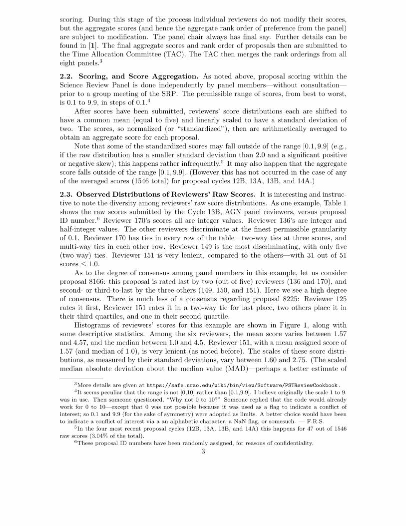
scoring. During this stage of the process individual reviewers do not modify their scores,but the aggregate scores (and hence the aggregate rank order of preference from the panel)are subject to modification. The panel chair always has final say. Further details can befound in [1]. The final aggregate scores and rank order of proposals then are submitted tothe Time Allocation Committee (TAC). The TAC then merges the rank orderings from alleight panels.3

2.2. Scoring, and Score Aggregation. As noted above, proposal scoring within theScience Review Panel is done independently by panel members—without consultation—prior to a group meeting of the SRP. The permissible range of scores, from best to worst,is 0.1 to 9.9, in steps of 0.1.4

After scores have been submitted, reviewers’ score distributions each are shifted tohave a common mean (equal to five) and linearly scaled to have a standard deviation oftwo. The scores, so normalized (or “standardized”), then are arithmetically averaged toobtain an aggregate score for each proposal.

Note that some of the standardized scores may fall outside of the range [0.1, 9.9] (e.g.,if the raw distribution has a smaller standard deviation than 2.0 and a significant positiveor negative skew); this happens rather infrequently.5 It may also happen that the aggregatescore falls outside of the range [0.1, 9.9]. (However this has not occurred in the case of anyof the averaged scores (1546 total) for proposal cycles 12B, 13A, 13B, and 14A.)

2.3. Observed Distributions of Reviewers’ Raw Scores. It is interesting and instruc-tive to note the diversity among reviewers’ raw score distributions. As one example, Table 1shows the raw scores submitted by the Cycle 13B, AGN panel reviewers, versus proposalID number.6 Reviewer 170’s scores all are integer values. Reviewer 136’s are integer andhalf-integer values. The other reviewers discriminate at the finest permissible granularityof 0.1. Reviewer 170 has ties in every row of the table—two-way ties at three scores, andmulti-way ties in each other row. Reviewer 149 is the most discriminating, with only five(two-way) ties. Reviewer 151 is very lenient, compared to the others—with 31 out of 51scores ≤ 1.0.

As to the degree of consensus among panel members in this example, let us considerproposal 8166: this proposal is rated last by two (out of five) reviewers (136 and 170), andsecond- or third-to-last by the three others (149, 150, and 151). Here we see a high degreeof consensus. There is much less of a consensus regarding proposal 8225: Reviewer 125rates it first, Reviewer 151 rates it in a two-way tie for last place, two others place it intheir third quartiles, and one in their second quartile.

Histograms of reviewers’ scores for this example are shown in Figure 1, along withsome descriptive statistics. Among the six reviewers, the mean score varies between 1.57and 4.57, and the median between 1.0 and 4.5. Reviewer 151, with a mean assigned score of1.57 (and median of 1.0), is very lenient (as noted before). The scales of these score distri-butions, as measured by their standard deviations, vary between 1.60 and 2.75. (The scaledmedian absolute deviation about the median value (MAD)—perhaps a better estimate of

3More details are given at https://safe.nrao.edu/wiki/bin/view/Software/PSTReviewCookbook .4It seems peculiar that the range is not [0,10] rather than [0.1,9.9]. I believe originally the scale 1 to 9.

was in use. Then someone questioned, “Why not 0 to 10?” Someone replied that the code would alreadywork for 0 to 10—except that 0 was not possible because it was used as a flag to indicate a conflict of

interest; so 0.1 and 9.9 (for the sake of symmetry) were adopted as limits. A better choice would have beento indicate a conflict of interest via a an alphabetic character, a NaN flag, or somesuch. — F.R.S.

5In the four most recent proposal cycles (12B, 13A, 13B, and 14A) this happens for 47 out of 1546raw scores (3.04% of the total).

6These proposal ID numbers have been randomly assigned, for reasons of confidentiality.

3

0 2 4 6 8 100.00

0.05

0.10

0.15

Reviewer 125

0 2 4 6 8 100.000.050.100.150.200.250.300.35

Reviewer 136

0 2 4 6 8 100.00

0.05

0.10

0.15

0.20

0.25

Reviewer 149

0 2 4 6 8 100.00

0.05

0.10

0.15

0.20

0.25

Reviewer 150

0 2 4 6 8 100.00.10.20.30.40.50.6

Reviewer 151

0 2 4 6 8 100.0

0.1

0.2

0.3

0.4

0.5

Reviewer 170

AGN Panel Raw Score Distributions, Cycle 13B H50 proposalsL

nr Mean Std Dev Skewness Kurtosis Median H-L Loc Scaled MAD Sn Qn

125 34 4.57 2.75 0.38 2.15 4.25 4.50 2.74 2.98 3.00136 25 3.20 1.77 0.85 3.42 3.00 3.00 1.48 1.86 2.10149 38 3.67 1.92 -0.01 2.34 3.85 3.70 1.85 2.03 2.02150 42 3.25 2.41 0.95 3.01 2.80 3.00 2.45 2.15 2.04151 48 1.57 1.62 1.97 6.68 1.00 1.25 0.82 0.83 1.03170 47 3.77 1.60 0.29 2.18 4.00 4.00 1.48 1.22 2.16

Figure 1. Histograms of Cycle 13B AGN proposal raw scores, by reviewer. The ordinate in each caserepresents the probability density.

the “typical” scale of a distribution such as Reviewer 151’s—varies between 0.82 and 2.74.)Three of the distributions (those of Reviewers 136, 150, and 151) show significant positiveskew.

Figures showing the raw score distributions from each of the eight review panels andthe four most recent proposal cycles (12B, 13A, 13B, and 14A) are given in Appendix B(Figures B-1 through B-8). Like Figure 1, these show for each panel/cycle pair (in columns 1through 6): the number of scores submitted by the given reviewer, the mean raw score,standard deviation, skewness, kurtosis, and median score. Columns 7 through 10 give a fewancillary statistics; these are defined in §2.4.

The reviewers’ raw score distributions shown in Appendix B are typically clusteredtoward the low end of the score range (i.e., higher ratings), and they often are positivelyskewed, with a few poor scores in the right-tail region. The average mean is 4.06 ± 0.85,the mean standard deviation is 1.85± 0.50, the mean skewness is 0.39± 0.48, and the meankurtosis is 2.63 ± 0.98. (For reference, the kurtosis of Gaussian, or normal distributionis equal to three; and for a normal distribution truncated at ±2.5σ about the mean thekurtosis is 2.6242.) Histograms of these statistics are shown in Figure 2. Table 2 liststhe number of proposals, by panel, for the four most recent proposal cycles. The typicalproposal is rated by five reviewers; out of the 1529 non-GMVA proposals, 17 were rated byonly two reviewers, 91 by three reviewers, 446 by four reviewers, 971 by five reviewers, andfour by six reviewers (the corresponding percentages are 1.1, 6.0, 29.2, 63.5, and 0.3).

Sometimes a reviewer’s score distribution is representative of a total ordering, or com-plete ranking of proposals, with no ties present. And sometimes reviewers appear to gradeon a curve. On the AGN Panel, Cycle 14A (see Figure B-1), Reviewer 149 has a scoredistribution which is exactly symmetric and contains no ties—in ascending order the 51

4

Cycle 13B, AGN Panel Raw Scores

— Reviewer 125 —

{8225} 0.1{8136} 0.5

{7943, 7965} 1.

{8193} 1.5{7939} 2.

{8051} 2.1{7905, 7924, 8055, 8164} 2.5

{7789} 3.

{7709, 7880} 3.5{7833, 8161, 8219} 4.

{7874, 7993, 8178} 4.5{7867} 4.8

{7827, 8176, 8231} 5.

{8249} 5.5{8061} 6.2{8025} 7.

{8247} 7.2{8172} 7.3

{8112, 8138} 8.

{7768, 7903, 8096} 8.5{7859, 8163} 9.9

— Reviewer 136 —

{7956, 8010, 8025} 1.

{7731, 7789, 8015} 1.5{7903, 7972, 8133, 8247} 2.

{7992, 8172, 8178} 2.5{7756, 8248, 8249} 3.

{8108, 8170} 3.5{7770, 7859, 7867, 7943, 7965, 8123} 4.

{8040} 5.

{7768, 8176} 6.

{8166} 8.

— Reviewer 149 —

{7874, 7993} 0.5{8161, 8219} 0.8{8112, 8193} 1.

{7709} 1.2{8108} 1.4

{7770, 7897} 2.

{7679} 2.5{8136} 2.8{8133} 3.

{7924} 3.2{7789} 3.3

{8015} 3.4{7992} 3.5{8055} 3.7{8170} 3.8{7965} 3.9{7880} 4.

{7903} 4.2{8040} 4.4{8225} 4.5{7833} 4.6{7905} 4.7{8138} 4.8

{8051, 8123} 4.9{8061} 5.

{7859} 5.2{8164} 5.3{7939} 5.5{8163} 5.7{7827} 6.

{8096} 6.5{8166} 7.

{8231} 8.

— Reviewer 150 —

{7993, 8010} 0.1{7874} 0.5

{7903, 7939, 7943, 8161, 8178, 8193, 8219, 8248} 1.

{8040} 1.2{8096} 1.5{7731} 1.8

{7897, 8136, 8164, 8247, 8249} 2.

{8138, 8170} 2.2{7827, 8025} 2.5

{7770, 8015, 8172} 2.8{7709, 8051} 3.

{7679} 3.1{8225} 3.2{8231} 3.5

{7924, 7992} 3.8{7833} 4.2{8055} 4.5

{7768, 8061, 8112} 5.

{7880} 5.2

{8176} 6.8{8123, 8133, 8166} 8.

{8163} 8.5{7905} 9.

— Reviewer 151 —

{8133, 8136} 0.1{7956, 8015} 0.2{7939, 7992} 0.3{7709, 8193} 0.4

{7768, 7770, 7827, 8096, 8108, 8112, 8164, 8170} 0.5{8055} 0.7

{7965, 8176} 0.8{7859, 8025} 0.9

{7731, 7789, 7874, 7880, 7972, 7993, 8123, 8138, 8247, 8248} 1.

{7756} 1.2{7833, 8178} 1.5

{8249} 1.6{7867, 7897, 7924, 8010, 8040, 8172} 2.

{8161, 8163, 8219} 2.5{7679, 7943} 3.

{7905, 8231} 4.

{8166} 5.5{8061, 8225} 7.

— Reviewer 170 —

{7874, 7993} 1.

{7709, 7789, 7833, 7992, 8010, 8055, 8133, 8161, 8178, 8219, 8231, 8247, 8248} 2.

{7897, 7903, 7924, 7956, 8108, 8136, 8225} 3.

{7731, 7756, 7768, 7770, 7859, 7867, 7905, 7939, 7943, 7965, 8015, 8025, 8123, 8164, 8193, 8249} 4.

{7827, 8170} 5.

{7679, 7880, 8061, 8096, 8112, 8138, 8163, 8172} 6.

{8040, 8166} 7.

Table

1.

Cycle

13B

,A

GN

pro

posa

lra

wsco

res,by

review

er.P

roposa

lID

num

bers

are

giv

enth

eleft-h

and

colu

mns,

and

the

corresp

ondin

gra

wsco

resin

the

right-h

and

colu

mns.

Multi-elem

ent

pro

posa

lID

listsco

rrespond

toa

multi-w

ay

tiefo

rth

egiv

ensco

re.N

ote

the

div

ersityam

ong

the

review

ers’perso

nalsco

redistrib

utio

ns.

The

quartile

valu

esfo

rth

esix

review

ersare:

Rev

iewer

125,

(2.5

,4.2

5,

7);

Rev

iewer

136,

(1.8

75,

3,

4);

Rev

iewer

149,

(2,

3.8

5,

4.9

);R

eview

er150,

(1.2

,2.8

,4.5

);R

eview

er151,

(0.5

,1,

2);

and

Rev

iewer

170,(2

,4,4.7

5).

5

0 2 4 6 8 100.0

0.1

0.2

0.3

0.4

0.5

0.6

Mean, All Raw Score Distributions

0 1 2 3 4 50.0

0.2

0.4

0.6

0.8

1.0

Std Dev, All Raw Score Distributions

-3 -2 -1 0 1 2 30.0

0.2

0.4

0.6

0.8

1.0

1.2

Skewness, All Raw Score Distributions

2 4 6 8 100.0

0.2

0.4

0.6

0.8

Kurtosis, All Raw Score Distributions

Figure 2. This Figure shows histograms of the mean, standard deviation, skewness, and kurtosis statisticsof all the reviewers’ raw score distributions combined for proposal semesters 12B, 13A, 13B, and 14A. Theaverage mean is 4.06 ± 0.85, the mean standard deviation is 1.85 ± 0.50, the mean skewness is 0.39 ± 0.48,and the mean kurtosis is 2.63± 0.98. Note that the distribution of the means is skewed to the left and thatof the skewnesses is skewed to the right.

scores are: a few scores separated in steps of 0.5, then a few separated by 0.3, then by0.2, then a bunch separated by 0.1, then the reverse of all that. Another example is ETPPanel Cycle 14A, Reviewer 114 (see Figure B-3). This score distribution, consisting of 21scores, is an exact fit (by Cramer–von Mises and Anderson–Darling tests) to a triangulardistribution over the range [0.5, 9.5]

2.4. Methodological Tools. In this section a few special methodological tools, suchas ancillary statistical measures, kernel density estimates, and “smooth” histograms aredescribed.

2.4.1. Hodges–Lehmann estimator. In the case of a skewed or fat-tailed distribution, thesample median might be viewed as better representative of the “most typical” value of anunderlying (or parent) distribution than the sample mean. A similar estimator, also basedon order statistics, is the so-called Hodges–Lehmann estimator of location [2]. This has asimple definition: it is the median of all the pairwise averages of x1, . . . , xn, i.e.,

med1≤i,j≤n

xi + xj

2. (1)

For independent samples from a continuous symmetric distribution, the H–L estimator is,in fact, an estimator of the population median. For fat-tailed distributions especially, ithas the advantage that it generally converges faster to the population median than doesthe sample median (i.e., it is often a more efficient estimator of the population medianthan the sample median itself). Also, the H–L estimator has a smooth influence function—i.e., if a sample value is varied continuously, this estimate of distribution centrality varies

6

AGN Panel

12B 13A 13B 14A Total

GBT 4 8 4 4 20VLA 33 16 24 31 104

VLBA�HSA 18 35 22 25 100GMVA 1 5 3 3 12Total 56 64 53 63 236

EGS Panel

12B 13A 13B 14A Total

GBT 13 15 11 22 61VLA 17 33 21 35 106

VLBA�HSA 3 0 1 2 6GMVA 0 0 0 0 0Total 33 48 33 59 173

ETP Panel

12B 13A 13B 14A Total

GBT 21 13 18 20 72VLA 26 23 21 30 100

VLBA�HSA 10 11 12 11 44GMVA 0 0 0 1 1Total 57 47 51 62 217

HIZ Panel

12B 13A 13B 14A Total

GBT 9 10 7 8 34VLA 35 34 42 51 162

VLBA�HSA 0 7 5 6 18GMVA 0 2 0 0 2Total 44 53 54 65 216

ISM Panel

12B 13A 13B 14A Total

GBT 19 25 22 26 92VLA 7 35 19 35 96

VLBA�HSA 2 0 1 0 3GMVA 0 0 0 0 0Total 28 60 42 61 191

NGA Panel

12B 13A 13B 14A Total

GBT 6 2 2 9 19VLA 22 39 30 35 126

VLBA�HSA 0 2 1 2 5GMVA 0 0 0 0 0Total 28 43 33 46 150

SFM Panel

12B 13A 13B 14A Total

GBT 13 12 11 2 38VLA 37 48 32 56 173

VLBA�HSA 4 4 2 3 13GMVA 0 0 0 0 0Total 54 64 45 61 224

SSP Panel

12B 13A 13B 14A Total

GBT 1 6 9 5 21VLA 19 25 25 24 93

VLBA�HSA 2 9 9 3 23GMVA 0 1 0 1 2Total 22 41 43 33 139

Table 2. Number of proposals, by panel, for recent review cycles 12B, 13A, 13B, and 14A. A total of1546 proposals underwent review: 357 for GBT, 960 for VLA, 212 for VLBA (including HSA), and 17 forGMVA time. The GMVA proposals are also reviewed by a European review panel; the final ranking for thiscategory of proposals, and the telescope time allocation, are done outside of the normal SRP and TAC.

continuously, unlike the sample median. Thus it can be viewed as a smooth version of themedian (see Rousseeuw and Croux (1993) [3]). Figure 3 (left) shows the distribution ofthe ratio of the mean score to H–L location estimate, including all reviewers’ raw scoredistributions for the four most recent proposal cycles.

2.4.2. Alternative measures of scale (or dispersion). Also for many non-Gaussian (e.g.,fat-tailed, skewed, or outlier-contaminated distributions) the standard deviation is an over-estimate of the “typical” dispersion of the distribution. The median absolute deviationabout the median value (the so-called MAD), scaled by a constant c, is commonly usedas an alternative measure of scale.7 However, the scaled MAD is only 37% efficient in thecase of the Gaussian distribution. Rousseeuw and Croux (1993) [3] define two alternativeauxiliary estimates of scale, which they term Sn and Qn, that achieve higher efficiency (58%and 81%, respectively) at the Gaussian distribution. Both of these are defined in terms of

7The value c = 1.4826 is chosen to make the scaled MAD asymptotically agree with the standarddeviation in the case of a Gaussian distribution.

7

0.90 0.95 1.00 1.05 1.10 1.15 1.20 1.250

5

10

15

20

Mean�H-L Location

0.6 0.8 1.0 1.2 1.4 1.6 1.80.0

0.5

1.0

1.5

2.0

2.5

3.0

Std. Dev.�Qn

Figure 3. At left is shown a histogram of the ratio of mean score to Hodges–Lehmann location estimate,including all reviewers’ raw score distributions for the four most recent proposal semesters. At right isshown the histogram of ratios of standard deviation to the Qn estimator of scale. The mean values of thesedistributions are 1.024 ± 0.043 and 1.035 ± 0.202, respectively.

order statistics on the set of pairwise absolute differences, {|xi − xj | ; i < j}.8,9 Like theMAD, the influence function for Sn has discontinuities—whereas the influence function forQn is smooth. Figure 3 (right) shows the distribution of the ratio of the standard deviationto Qn estimate of scale, including all reviewers’ raw score distributions for the four mostrecent proposal cycles.

2.4.3. Kernel density estimates and “smooth histograms”. We show in Figure 1 and Appen-dices B and C, in addition to the traditional histogram, a smooth curve representing someputative, underlying probability density function (PDF), for each of the given raw scoredistributions. These smooth curves are based on the so-called kernel density estimator, asdescribed by Silverman (1986) [4]. The method is easy to describe: Given data samplesx1, x2, . . . , xn, place a unit mass at the abscissa of each data sample, convolve the resultingsum of δ-distributions with a smooth, non-negative kernel (e.g., a Gaussian) of appropri-ately chosen width, and normalize so that the resulting smooth function integrates to unity.Expressed mathematically, the kernel density estimate is given by

f(x) =1

nh

n∑

i=1

K

(x − xi

h

), (2)

where K is the kernel function and h is the bandwidth.The plot of a kernel density estimate is sometimes referred to as a “smooth histogram”.

This is the terminology used in Mathematica. For the curves shown in this memorandum weuse the Mathematica implementation of kernel density estimates, with a Gaussian kernel.The kernel bandwidth is chosen adaptively. For bandwidth selection we choose, variously, amethod due to Scott—or another by Silverman—both are implemented within Mathematica.And for the traditional histogram, we select a bin width commensurate with the bandwidthof the adaptive kernel density estimate.

The smooth histogram resulting from a kernel density estimator has a major advantageover its traditional counterpart, in that the traditional histogram can be overly sensitive to

8Sn is defined via Sn = c lomedi{himedj |xi − xj |}, where lomed is the ⌊(n + 1)/2⌋th order statistic,himed is the (⌊n/2⌋ + 1)st order statistic, ⌊·⌋ denotes the greatest integer (or floor) function, and c =1.1926. Additionally, a bias correction is applied which, in the case of Gaussian-distributed data, makesthis estimator unbiased for small sample sizes.

9Qn is defined via the kth order statistic of pairwise differences: Qn = d {|xi − xj | ; i < j}(k), where

k =`

h

2

´

, h = ⌊n/2⌋ + 1, and d = 1.0483. A bias correction is applied, as in the case of Sn.

8

choice of origin—or choice of bin locations, in general.10 The smooth histogram is sensitiveto neither. The most powerful modern methods for tests of multi-modality are based onkernel density estimates [4]. One disadvantage of smooth histograms is that long-taileddistributional detail may not show up as well as with a traditional histogram (though adata-adaptive variable bandwidth choice, dependent on local density, may overcome thisdisadvantage).

2.4.4. Quantitative comparison of score distributions. Since the end product of panel reviewis a rank-ordered list of proposals based on final scores, quantitative rank-order comparisonsof score distributions (e.g., one reviewer vs. another, or one scoring method vs. another)are very apt. For lists of equal length, the Kendall τ and Spearman ρ measures of rankcorrelation are commonly used. Definitions for these vary slightly; we use the tie-correctedversions that are implemented in the standard Mathematica library. The ρ and τ valuescan vary over the range [−1, 1] (+1 if the rank orderings are identical, −1 if they are thereverse of each other, 0 for no association).

Langville and Meyer [5] introduce a modified Kendall τ which can be used for compar-ison of partial lists (e.g., top-k lists). The so-called Spearman weighted footrule is definedanalogously to Spearman’s ρ, but assigns higher weight to discrepancies at higher rankorders.

2.5. Comments and Recommendations. In this section we offer a few suggestions forminor modifications of the proposal scoring system.

1. Adjustment of scale of reviewers’ score distributions. In Appendix B we saw that thereviewers’ raw score distributions often are skewed. For such distributions, the standarddeviation tends to be an over-estimate of the typical spread between scores. Perhaps use ofthe scaled MAD, Sn, or Qn should be used for normalization of the score distributions, inlieu of the standard deviation. We would suggest the use of Qn, which is based on pairwisedifferences of scores, has high efficiency and a smooth influence function, and—unlike thestandard deviation or the MAD—is a scale estimate which does not depend on a priorestimate of location (e.g., mean or median).

If this change were made, however, there would be more occurrences of scores outsidethe range [0, 10] because the influence of scores in the tail of a narrow, skewed, raw scoredistribution would increase. One might prefer to truncate the distribution of normalizedscores to the [0, 10] range.

2. Shift of the reviewers’ score distributions. Likewise, we might consider use of the medianor the H–L location estimate of each reviewer’s score distribution—rather than the samplemean—for alignment of reviewers’ score distributions in the score normalization process.But we believe the effect would be relatively minor compared with that of Suggestion #1,given the nature of the ratio distributions shown in Figure 3.

3. Use of data from all cycles for score normalization. Each reviewer ordinarily serves fortwo years (four consecutive semesters). In Appendix B we see—for a given reviewer—afair degree of consistency between score distributions from consecutive semesters. Hencewe might consider normalizing over previous semesters, as well as the immediate one, forcalibrating reviewers’ scores. However, if reviewers were at some point to be given revisedscoring guidelines, this idea would certainly be ruled out (except for following semesters).

4. Normalization of panel chair’s score distribution. One should note that, because thepanel chair votes only when another member of the panel is conflicted, there often will be

10This can be especially the case if the data are quantized. (As they are, in our case.)

9

a paucity of scores from the panel chair, and therefore a relatively poorer calibration thanfor other reviewers. Incorporation of Suggestion #3 could help somewhat.

5. Should panel chairs always vote (except when conflicted)? If the panel chairs were tovote on all their panel’s proposals, then—obviously—there would be better calibration fortheir scores, and, typically, five or six reviewers per proposal, rather then four or five. Therationale for the current scheme is probably (1) that the panel chair should not have theadditional burden, beyond his or her organizational duties, of scoring every proposal, and(2) possibly, that the chair should not be given additional power. Whatever the rationale,we feel it ought to be elucidated somewhere.

6. Reviewer effort expended in resolving minor score differences. Some reviewers, in spiteof having a large number of proposals to review (50 or 60+ in some cases), produce rawscore distributions which are either completely free of tie scores—equivalent to a totalrank ordering of the proposals—or very nearly free of ties. It almost surely takes iterationto achieve this level of discrimination, and we do not believe it is worth the effort todiscriminate this finely between similarly ranked proposals. Reviewers perhaps should beinstructed not to worry about minor score differences—that differences with respect to theother panelists’ scores will likely overweigh the fine tuning of one’s own scores.

7. Point scale. Along this same vein of reasoning: if the point scale had coarsergranularity—e.g., permitting only integer, or integer and half-integer scores—then reviewerswould not be able to discriminate so finely as now between similarly ranked proposals,11

and this restriction could possibly reduce the reviewers’ exertion of effort, lessening theirburden.

8. Rating one’s own competence to review a given proposal. In some review systems,particularly for journal or conference paper refereeing, reviewers are asked to rate their ownlevel of expertise in scoring the assigned paper or proposal (perhaps on a coarse scale ofone to three). See Haenni (2008), [6]. These self-confidence levels can then be factored in,via appropriate weighting, when computing an aggregate score for each proposal. At firstglance, since we have eight expert SRP panels rather than one; our expectation might bethat every panel member is fully qualified to review every proposal. But perhaps this ideais worth consideration.

This could alleviate some of the burden on reviewers by relieving them of the need toagonize over score decisions in sub-specialty areas that they are not totally familiar with.It could lessen their embarrassment in the face-to-face panel review if they have been toosqueezed for time to fully research every proposal. Also it could alleviate, somewhat, theneed for score modifications in the SRP group meeting—and thus make the process moreeffective and objective, overall.

9. Grading on a curve. The current normalization scheme does not modify the shape of areviewer’s score distribution (recall that it only shifts and linearly stretches or shrinks it).A simple alternative would be to grade on a curve: i.e., to modify each reviewer’s scoredistribution to match the percentiles of some target distribution, say, a truncated normaldistribution with a mean of five and standard deviation equal to two.

Another possibility would to choose as the target distribution the mean raw scoredistribution, averaging over all reviewers in the panel. That way, the scores of a “typical”reviewer (say, with a mean near 4.0, a standard deviation near 1.85, the typical positiveskew, and few outliers) would be minimally altered. (See Section 5, below.)

11For example, if the scores were restricted to half-integer scores in the range [.5, 9.5], then there wouldbe only 19 distinct possible raw scores, as opposed to 99.

10

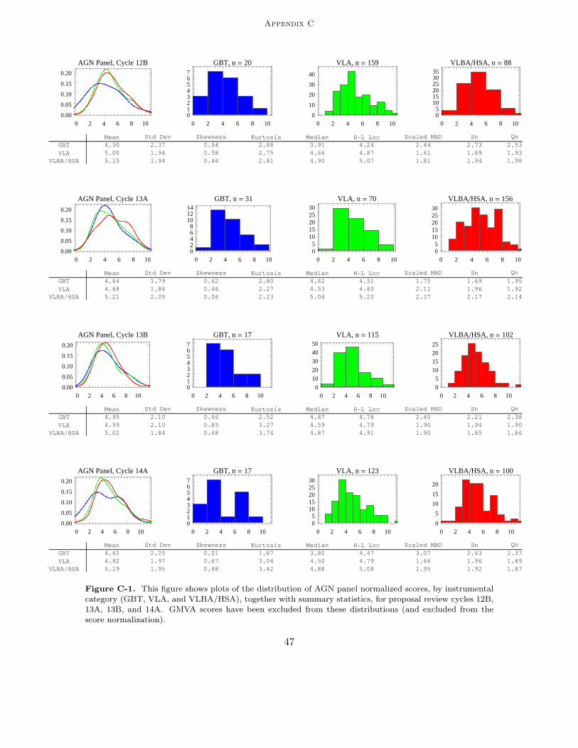
2.6. Discussion. At a recent NRAO scientific staff meeting, concerns were raised aboutthe appropriateness of proposal review combining all three instrumental categories (GBT,VLA, VLBA), as opposed to having separate review panels for each of these categories.The consolidated review is likely more economical than the alternative, and it is more inaccord with the prevailing “One Observatory” philosophy. But one might argue that eachinstrument ‘deserves’ its own dedicated review structure.12 A specific concern that wasraised was that, given the premier capabilities of the GBT for pulsar studies, meritoriousproposals for pulsar studies using unique capabilities of the VLA might be unfairly out-competed by GBT proposals in the consolidated review (within the ETP panel). In light ofthis we have taken a detailed look at the distribution of normalized scores, by instrument, forthe four most recent review cycles. Histograms of these distributions, along with summarystatistics, are shown in Appendix C. The cumulative distributions are shown in Appendix D,together with distributional two-sample test statistics (Kolmogorov–Smirnov, Cramer–vonMises, and Anderson–Darling P -values) showing pairwise comparisons: GBT vs. VLA, GBTvs. VLBA, and VLA vs. VLBA.

In Appendix E we compare, for each of the SRPs, the initial rank-order aggregatepreferences vs. the rank order after SRP meeting score adjustments. (Since only the ag-gregated scores are adjusted, as opposed to individual reviewers’ scores, c.d.f. comparisonslike those of Appendix D are not possible.) We were surprised by the large number of scoreadjustments and rather extreme rank-order excursions which are seen in some cases (e.g.,NGA panel, semester 13A).

3. Comparison with Procedures Used Elsewhere

[Note: We apologize that this section is incomplete. We will try to make an updatedversion available.]

European Southern Observatory. An ESO working group undertook a review of their pro-posal selection process in 2012. The group report, and an accompanying study of thegrowth of observing programs at ESO, were published in the December 2012 issue of theESO Messenger [15, 16]. Their review system includes thirteen panels, with six memberseach, to cover four science categories: Cosmology (three panels); Galaxies and Galactic Nu-clei (two panels); ISM, Star Formation, and Planetary Systems (four panels); and StellarEvolution (four panels). Proposals for all the ESO telescopes, at Paranal and LaSilla, aswell as APEX, are reviewed by the same panels. They review typically 1000 proposals persemester, with an average of approximately 70–80 proposals per panel. Their review processis structured similarly to ours. The rating scale is 1 to 5 (low is best), with a granularityof 0.1. The bottom 30% of proposals are “triaged” (i.e., not considered in the post-ratingpanel discussion).13

Additional details are given in [17]. One notable differences from the NRAO reviewprocess is that, in committee, revised scores for proposals are submitted by each reviewer,and this is done by formal written ballot. These scores then are averaged to arrive atthe group consensus (in contrast to the procedure in the NRAO SRPs, where there is noprescribed procedure for score adjustment). Also, apparently, separate votes are taken pertelescope.

ALMA. For ALMA proposals there are five science categories (Cosmology and the high-zuniverse; Galaxies and galactic nuclei; ISM, star formation and astrochemistry; Circum-

12Similar concerns have been raised concerning ESO proposal review. See [15].13However, according to [17] there is a mechanism by which a panel may request that a triaged

proposal be “resurrected”.

11

stellar disks, exoplanets, and solar system; and Stellar evolution and the Sun) [18]. Thereare eleven review panels (two for category 1; three each for categories 2 and 3; two forcategory 4; and one for category 5), with seven members per panel. Initially each proposalis rated by four reviewers. The range of scores is 1 to 10 (low score is best). Each reviewer’sraw score distribution is normalized to a common mean and variance. The last 30% aretriaged, and not considered further by the review committee. Otherwise, the initial scoresare taken as recommendations only. A final rank-ordering of proposals is arrived at byconsensus of the panel members.

Arecibo Observatory. Arecibo has a similar panel structure and similar review procedure.They use a scale of 1 to 9; high numerical score is best.

Hubble Space Telescope.

NOAO.

National Science Foundation and National Institutes of Health. Proposal review proce-dures in use at NSF are not uniform across the various divisions of the agency, accordingto Robert L. Dickman and William E. Howard III (private communication). Based oninformation from the Web, it appears that relatively more uniform procedures have beenadopted by NIH than by NSF.

According to Hal R. Arkes (2003) [20], in 1994 the GAO issued a report with anevaluation of the review procedures at NSF and NIH. With regard to NSF, the authorsof this report “were concerned that the stated criteria by which NSF proposals should beevaluated were not, in fact, the only criteria by which such proposals were evaluated. . . .[and] the GAO ‘stated that we found that unwritten or informal criteria were used by panelsat all three agencies’.” In the 1994–1995 time period, according to Arkes, both NSF andNIH were revamping their review processes, and he was involved with both efforts.

Arkes chose to examine one of the grant review processes, in which each reviewer (outof four, total) was asked to submit numerical scores on each of four specific criteria, and alsoto submit an overall score. He found, by regression analysis (for 70 proposals), that, whilethree out of four reviewers’ overall scores agreed with their scores on the individual criteria(R2 values between 0.80 and 0.95, accounting for a large proportion of the variance in theoverall ratings), one reviewer was not consistently using these four criteria in generating anoverall rating (R2 = 0.28).

Apparently, in the mid-90s NSF and NIH review panels were not generally using scorenormalization. Arkes suggested using z-scores, i.e., standardizing to normal distributionwith a mean of zero and a standard deviation equal to one. This is entirely equivalent toour normalization procedure.

His second suggestion was that proposals be “triaged” before panel discussion (similarlyto the ESO procedure), i.e., to generate “cut-off” scores, so that panelists would not needto discuss proposals that had no chance of funding.

His final suggestion was to use what he termed “disaggregated” reviewers’ ratings—i.e., have the reviewers score only on the the individual criteria, and not submit an overallscore—the argument being that this would make it more likely that solely official criteriawould be used.

The NSF rejected all three of his recommendations (including score normalization).NIH around this time period utilized a 150-point scoring system. Arkes cites psycho-

logical research studies which he said show that “if points on rating scales extend beyondapproximate seven”, rater reliability either drops or fails to increase. Other consultants, hesays, were also recommending that the scale be trimmed.

The only recommendation that NIH adopted was to explicitly request the reviewers12

to rate by each criterion. And they considered score normalization to be too difficult toimplement.

From current Web documentation we find that NIH now asks reviews to score on ascale of 1 to 9. They must provide both an overall impact score and scores on, typically,five specified criteria. The guidelines state specifically that the impact score is not intendedto be an average of criterion scores. Reviewers may modify their initial scores during thepanel review meeting.

4. Rating Aggregation Methods Based on Pairwise Score Comparisons

There is a great deal of current interest in rating and ranking methods, and a large,rapidly growing literature. A comprehensive survey on the subject is given by Amy N. Lang-ville and Carl D. Meyer in a book titled Who’s #1? The Science of Rating and Ranking,published by Princeton University Press in 2012 [5]. There the concentration is on algebraicand graph-theoretic methods (rather than classical or Bayesian statistical methods) whichare widely used today in fields such as sports team ranking, e-commerce (e.g., Amazon,Netflix, most major retailers), and information search and retrieval (e.g., Google).14 Algo-rithmic techniques based on the same theory as these can be used for aggregating the scoresof journal referees or proposal reviewers. On pp. 179–181 of Langville and Meyer there isan aside titled “Ranking NSF Proposals”. Below we will show the result of applying theirsuggested method to the AGN Panel, Cycle 13B reviewers’ scores.

The method they propose is based on the Perron–Frobenius theorem (which dates backto 1907–1912) on the eigenvalues of real, square, non-negative, irreducible15 matrices. Thefoundations for methods of this type were established around the early 1950s (see [7]): byJohn R. Seeley (1949); by T.-H. Wei (1952), a student of the famous statistician MauriceKendall at Cambridge University, in a Ph. D. dissertation titled The Algebraic Foundationsof Ranking Theory; and by Kendall (1955). The idea is that given n entities to compare andan n×n matrix M expressing by how much entity i is favored over entity j (or vice-versa),for all pairs i and j, the normalized eigenvector corresponding to the dominant eigenvalueof M provides the correct ranking. So, for each of m reviewers one can construct a squarematrix Mk of pairwise score differences; i.e., in row i column j of the matrix one has thescore differential |s(i) − s(j)|, if proposal i is rated above proposal j, and 0 otherwise.One normalizes each Mk by dividing by the sum of all entries. (It does not matter if thereviewer has not scored all proposals.) Then one forms the average of these matrices andfind the dominant eigenvector. Assuming the matrix is irreducible (which it will be unlessthe review assignments are inadequate) the Perron–Frobenius theorem guarantees that theelements of the dominant eigenvector will be non-negative. These elements then representthe aggregated scores of the reviewers, according to the theory of Wei et al.

Results using the Langville–Meyer method. Figure 4 shows a comparison between our usualmean standardized scores and the scores obtained using the Langville–Meyer formulationof the method above. The comparison is by means of bipartite score plots. Proposal IDnumbers are shown along the vertical axes. In general, the quartile memberships agreefairly well, but we were surprised by the number of relatively large jumps in rank (which weobserved also for other cycle/panel pairs). In the case of Proposal 8051, we see a jump fromthe third quartile to the first, and for Proposal 7756 we see a similarly large jump—bothof these proposals were rated by only three reviewers. In the first quartile, Proposal 7972

14Google’s CEO Larry Page (a computer scientist) has a net worth of around $31 billion, largely dueto the success of his PageRank algorithm which is at the heart of the Google search engine.

15The definition is somewhat technical.

13

jumps eight places higher in ranking—this proposal was rated by only two reviewers. ForCycle 13B, AGN, the distribution number of reviewers per proposal is as follows: just oneproposal had only two reviewers, three proposals had just three reviewers; seven proposalshad four reviewers, and thirty-nine proposals had five reviewers. The percentages are:2 reviewers, 2%; 3 reviewers, 6%; 4 reviewers, 14%; and 5 reviewers, 78%.

Results using a method due to Gleich and Lim. Another approach to the aggregation ofratings or scores is described by David Gleich and Lek-Heng Lim in [8] and Jiang et al. [9].We summarize the Gleich and Lim process as follows: They begin by noting a connectionto skew-symmetric matrices.16 Given a column vector of n scores s = (s1, . . . , sn)T , thematrix Y of pairwise score differences Yij = si − sj is skew-symmetric. Assuming Y 6= 0,Y is of rank two, since it can be written in the form

Y = s eT − e sT , (3)

where e is a column vector of n ones. Suppose one were given a measured version Y of thatmatrix, contaminated by noise and perhaps missing some elements. In that case, one could

solve for a low-rank, skew-symmetric approximation to Y which is, in some well-defined

sense,17 closest to Y. (We denote the kth individual reviewer’s pairwise score differencematrix by Y(k).)

This is an example of the so-called matrix completion problem, which is a bit of ahot topic these days, as it arises in contexts such as compressive sensing. Algorithms formatrix completion are discussed by Gleich and Lim in [8, Section 3]. They treat the specialproblem of matrix completion restricted to the class of skew-symmetric matrices. Supposewithin a panel we have m reviewers of n proposals, whose scores—or ratings—are given by

an m × n matrix R. We then can form an n × n matrix Y whose elements represent thearithmetic means of reviewers’ pairwise score differences, i.e.,

Yij =

∑m

k=1(Rki − Rkj)

# {k |both Rki and Rkj exist}, (4)

where #{·} denotes the cardinality of the given set,18 and in the case of a denominator

equal to 0, we set Yij = 0. In our case, Y is not an exact pairwise difference matrix becausenot all m reviewers review all proposals.

In Section 3.1 of their paper, Gleich and Lim use the singular value projection algorithm

of Jain et al. [10], to find a rank-2 skew-symmetric approximation Y which is nearest to

16An n × n real matrix M is skew-symmetric if M = −MT.17As measured, say, by a matrix norm.18Gleich and Lim include a few other possibilities: Rather than the arithmetic mean of score differ-

ences, one might choose the (log) geometric mean of score ratios; i.e.,

bYij =

Pmk=1(log Rki − log Rkj)

k |both Rki and Rkj exist¯ ;

or binary comparison, in which case, Y(k)i,j = sign(Rkj − Rki) and

bYi,j = Probk

(Rki > Rkj) − Probk

(Rki < Rkj) ;

or the logarithmic odds ratio, with bYij = logProbk (Rki ≥ Rkj)

Probk (Rki ≤ Rkj).

14

7679

7709

7731

7756

7768

7770

7789

7827

7833

7859

7867

7874

7880

7897

7903

7905

7924

7939

7943

7956

7965

7972

7992

7993

8010

8015

8025

8040

8051

8055

8061

8096

8108

8112

8123

8133

8136

8138

8161

8163

8164

8166

8170

8172

8176

8178

8193

8219

8225

8231

7679

77097731

7756

7768

7770

7789

7827

7833

7859

7867

7874

7880

7897

7903

7905

7924

7939

7943

7956

7965

7972

7992

79938010

8015

8025

8040

8051

8055

8061

8096

8108

8112

8123

8133

8136

8138

8161

8163

8164

8166

8170

8172

8176

8178

8193

8219

82258231

9.34758

2.97524

9.9

0.1

MStd Langville-Meyer

7679

7709

7731

7756

7768

7770

7789

7827

7833

7859

7867

7874

7880

7897

7903

7905

7924

7939

7943

7956

7965

7972

7992

7993

8010

8015

8025

8040

8051

8055

8061

8096

8108

8112

8123

8133

8136

8138

8161

8163

8164

8166

8170

8172

8176

8178

8193

8219

8225

8231

7679

77097731

7756

7768

7770

7789

7827

7833

7859

7867

7874

7880

7897

7903

7905

7924

7939

7943

7956

7965

7972

7992

79938010

8015

8025

8040

8051

8055

8061

8096

8108

8112

8123

8133

8136

8138

8161

8163

8164

8166

8170

8172

8176

8178

8193

8219

82258231

9.34758

2.97524

9.9

0.1

MStd Langville-Meyer

Figure 4. Comparison between mean standardized scores and scores obtained using the Langville–Meyeralgorithm [5, pp. 179 ff.] for the Cycle 13B, AGN Panel. In the plot at left, the vertical scale is linear, fromminimum score (top) to maximum (bottom). (The Langville–Meyer dominant eigenvector scores have beenscaled to the range [0.1, 9.9].) At right, the score distances are ignored; i.e., the comparison is solely byrank order. The first quartile scores are shown in green, the second in blue, etc. Dashed lines correspond

to inter-quartile jumps.

15

7679

7709

7731

7756

7768

7770

7789

7827

7833

7859

7867

7874

7880

7897

7903

7905

7924

7939

7943

7956

7965

7972

7992

7993

8010

8015

8025

8040

8051

8055

8061

8096

8108

8112

8123

8133

8136

8138

8161

8163

8164

8166

8170

8172

8176

8178

8193

8219

8225

8231

7679

7709

7731

7756

7768

7770

7789

7827

7833

7859

7867

7874

7880

7897

7903

7905

7924

7939

7943

7956

7965

79727992

7993

8010

8015

8025

8040

8051

8055

8061

8096

8108

8112

8123

8133

8136

8138

8161

8163

8164

8166

8170

8172

8176

8178

8193

8219

8225

8231

9.34758

2.97524

9.9

0.1

MStd Gleich-Lim

7679

7709

7731

7756

7768

7770

7789

7827

7833

7859

7867

7874

7880

7897

7903

7905

7924

7939

7943

7956

7965

7972

7992

7993

8010

8015

8025

8040

8051

8055

8061

8096

8108

8112

8123

8133

8136

8138

8161

8163

8164

8166

8170

8172

8176

8178

8193

8219

8225

8231

7679

7709

7731

7756

7768

7770

7789

7827

7833

7859

7867

7874

7880

7897

7903

7905

7924

7939

7943

7956

7965

7972

7992

7993

8010

8015

8025

8040

8051

8055

8061

8096

8108

8112

8123

8133

8136

8138

8161

8163

8164

8166

8170

8172

8176

8178

8193

8219

8225

8231

9.34758

2.97524

9.9

0.1

MStd Gleich-Lim

Figure 5. Comparison between mean standardized scores and scores obtained using the Gleich–Lim algo-rithm [8] for the Cycle 13B, AGN Panel. Here we see essentially identical memberships in the first quartile

(the only exception being proposals 7972 and 8178, which stay very close to the quartile boundary), andwe see identical memberships in the fourth quartile. There are two pairs of exchanges between the secondand third quartiles.

16

Y in the sense of the so-called nuclear norm. The nuclear norm is the matrix equivalentof the discrete ℓ1 vector norm. It is also known as the trace norm, or in physics a Ky-Fannorm. For a general real matrix A, the nuclear norm is simply the sum of the singularvalues of A; the singular values are equal to the square roots of the non-zero eigenvalues of

AT A. Given the minimum norm solution Y, the aggregate scores from the algorithm are

s = (1/n)Ye (which we rescale to cover the range [0,10]). A Matlab implementation of thisalgorithm can be found among the research codes available at David Gleich’s home page.19

We used our own Mathematica implementation.

Figure 5 shows a comparison between the mean standardized scores and scores obtainedusing the Gleich–Lim algorithm for the Cycle 13B, AGN Panel. Here we see rather lessextreme differences than in the comparison with Langville–Meyer scores (Fig. 4).

5. A Quadratic Programming Method and a Probabilistic

Score Normalization Algorithm for Score Aggregation

In this section we briefly describe two approaches from the recent literature on cali-brating and aggregating reviewers’ scores. These algorithms assume that high scores arebest, so we would need to additively invert the input raw scores (s 7→ 10 − s), and invertthe output aggregate scores as well.

5.1. The Method of Roos et al. Two interesting papers on calibrating the scores ofbiased reviewers were published in 2011 and 2012 by Roos et al., [11, 12]. These authorsfirst describe a standard linear modeling approach, referred to in the statistical literature,as two-way cross-classification in the analysis of variance (ANOVA), that can be solved bylinear least squares if all reviewers review all proposals. The score model

yij = µ + αi + βij + ǫij (5)

is additive, consisting of the overall mean score µ, the mean difference αi between thescores of reviewer i and µ, the mean difference βj between the scores of proposal j andµ, and a random error ǫij . The errors are assumed to be independent and identicallydistributed (i.i.d.). The solution parameters are the αi, which can be thought of as reviewerlenience parameters, and the βj , which are estimates of intrinsic proposal quality. Forranking n proposals it suffices to have estimates of the quality difference with respect toone chosen proposal, say βi−β1. For the imbalanced case, in which reviewers score differingsubsets of all proposals, a constrained least-squares solver is required, with the constraints∑

i αi = 0 and∑

j βj = 0. This algorithm is inadequate for our purposes, because it doesnot include a multiplicative scale factor.

The authors next describe a nonlinear model

yij = µ + γi(αi + βij + ǫi,j) (6)

which does include scale factors, the γi. With the substitution γi = 1/γi, the least-squaresobjective function becomes

i,j

(yij γi − µγi − αi − βj)2 . (7)

19URL: https://www.cs.purdue.edu/homes/dgleich/codes/

17

7679

7709

7731

7756

7768

7770

7789

7827

7833

7859

7867

7874

7880

7897

7903

7905

7924

7939

7943

7956

7965

7972

7992

7993

8010

8015

8025

8040

8051

8055

8061

8096

8108

8112

8123

8133

8136

8138

8161

8163

8164

8166

8170

8172

8176

8178

8193

8219

8225

8231

7679

7709

7731

7756

7768

7770

7789

7827

7833

7859

7867

7874

7880

7897

7903

7905

79247939

7943

7956

7965

7972

7992

79938010

8015

8025

8040

8051

8055

8061

8096

8108

8112

8123

8133

8136

8138

8161

8163

8164

8166

8170

8172

8176

8178

8193

8219

8225

8231

9.34758

2.97524

8.97151

2.48848

MStd Roos

7679

7709

7731

7756

7768

7770

7789

7827

7833

7859

7867

7874

7880

7897

7903

7905

7924

7939

7943

7956

7965

7972

7992

7993

8010

8015

8025

8040

8051

8055

8061

8096

8108

8112

8123

8133

8136

8138

8161

8163

8164

8166

8170

8172

8176

8178

8193

8219

8225

8231

7679

7709

7731

7756

7768

7770

7789

7827

7833

7859

7867

7874

7880

7897

7903

7905

79247939

7943

7956

7965

7972

7992

79938010

8015

8025

8040

8051

8055

8061

8096

8108

8112

8123

8133

8136

8138

8161

8163

8164

8166

8170

8172

8176

8178

8193

8219

8225

8231

9.34758

2.97524

8.97151

2.48848

MStd Roos

Figure 6. Comparison between mean standardized scores and scores obtained using the Roos quadraticprogramming algorithm [11] for the Cycle 13B, AGN Panel.

18

Defining a vector x = (β1, . . . , βn, γ1, . . . , γm, α1, . . . , αm), one ends up with the quadraticprogramming problem:

minimize1

2xT Qx

subject to Ax ≥ b ,(8)

where the n × n matrix Q and the constraint matrix A both derive from Equation 7 andthe condition that 1

m

∑γi = 1. The solution can be obtained using existing solvers for

bound-constrained quadratic programming. Roos et al. used the Matlab MINQ; we usedthe Mathematica FindMinimum (which is actually a general-purpose solver). The solutionis the maximum likelihood estimate if the ǫij are i.i.d. Gaussian. A sample result is shownin Figure 6.

.

5.2. Grading on a Curve: The Method of Fernandez, Vallet, andCastells. Fernandez et al. in 2006 published a paper [13] on the topic of probabilisticscore normalization for rank aggregation. Their method consists in precisely matching thepercentage points of each reviewer’s raw score distribution to those of some common targetdistribution, then arithmetically averaging the scores so obtained. Thus it can be thoughtof as an extreme form of “grading on a curve”.

In their own application, in information retrieval, these authors appear to have specificgrounds to favor one target distribution over another, which are not relevant to our ownapplication. However, it occurred to us that it might be interesting in our application toapply this method, choosing as target distribution the mean distribution of raw scores,averaging over all reviewers within the given SRP for the given semester. Our rationale isthat, in this case, the “typical” reviewer would see relatively less difference with respectto his or her initial scores.20 Another thought would be to choose as target distributiona parametrized, bounded distribution (covering the range [0,10]) with similar first fourmoments (mean, standard deviation, skewness, and kurtosis) to the mean score distributionshown in our Figure 2.

The mathematics of this method can be described succinctly: Let F denote the cu-mulative distribution (c.d.f.) of the target distribution, let F (−1) denote the inverse c.d.f.,and let Fr denote the empirical c.d.f. of the reviewer’s raw score distribution. Then thetransformation from raw score to normalized score is

snormalized = F (−1)(Fr(sraw)

). (9)

A sample result is shown in Figure 7.

6. A Proposal by Merrifield and Saari for Distributed Peer Review

We would like to call attention to a 2009 paper by Michael Merrifield and DonaldSaari [14] who advocate an alternative, distributed approach to peer review of telescopeproposals. (Merrifield has served as a member of the ESO proposal review committee.)Their approach would spread the task of proposal review across the user community byrequiring each PI to review a certain number, m, of other proposals. That number mightbe m = 10, for example. (For each additional proposal with the same PI, he or she wouldbe given another m review assignments.) Conflicts of interest would be declared, as usual,in which case alternate assignments would be made. The major advantages are:

(1) that no one would be burdened by the task of reviewing a very large number ofproposals;

20And be less likely to grumble.

19

(2) that the model is scalable: if the number of proposals increases, the number ofreview assignments, per reviewer, does not;

(3) that each proposal would be reviewed by the same number of reviewers—conflictsof interest would not reduce that number; and

(4) that instrument-by-instrument proposal review (GBT, VLA, and VLBA/HSA, eachseparately) would be more affordable than under the traditional review panel model.

Each PI would be required to perform his or her full list of assignments; failure to do sowould result in disqualification of the PI’s own proposal(s). Thus, the workload wouldbe distributed evenly, and, as the authors point out “there is a disincentive to taking thelottery-ticket approach to telescope applications.” And the views of the entire communitywould be taken into account. Consensus rank-order preferences would be assigned using arank-aggregation of the type discussed in Section 4 of this report. Various safeguards wouldbe built-in, in order to award good refereeing.

Brinks et al. [15] report that the ESO working group on ran a test on the method.NSF is sponsoring a pilot study within their Sensors and Sensing Systems program. ThePI on that study, George Hazelrigg, an NSF official, reports that the response to the initialcall for proposals was well-received (private communication).

7. Discussion

With regard to proposal scoring and score aggregation we conclude that:

(1) We are not out of the mainstream, with respect to the procedures used by otherobservatories and at the federal science agencies; however,

(2) Our score aggregation procedure is behind the current state of the art, as exempli-fied by the modern rating and ranking theories—developed by mathematicians andcomputer scientists—that are widely used in the corporate world.

In Section 2.5 we offered suggestions for minor modifications of the current score normal-ization and aggregation procedure. We believe these suggestions should be given carefulconsideration. However, we do not strongly advocate that the alternative score-aggregationprocedures discussed in Section 4 should be adopted. This is because the practical differ-ence from these might well be “in the noise,” in comparison to the score adjustments thatare made in the SRP Panel meetings. (We do note, however, that any of the alternativemethods would be an easy plug-in replacement for the current score-aggregation module.)

On the other hand, if the External Review Committee were to recommend that a higherdegree of reliance be placed on the initial, independently derived SRP scores, then thesemore “sophisticated” score-aggregation methods should be considered.

20

7679

7709

7731

7756

7768

7770

7789

7827

7833

7859

7867

7874

7880

7897

7903

7905

7924

7939

7943

7956

7965

7972

7992

7993

8010

8015

8025

8040

8051

8055

8061

8096

8108

8112

8123

8133

8136

8138

8161

8163

8164

8166

8170

8172

8176

8178

8193

8219

8225

8231

7679

7709

7731

7756

7768

7770

7789

7827

7833

7859

7867

7874

7880

7897

7903

7905

7924

7939

7943

7956

7965

7972

7992

7993

8010

8015

8025

8040

8051

8055

8061

8096

8108

8112

8123

8133

8136

8138

8161

8163

8164

8166

8170

8172

8176

8178

8193

8219

8225

8231

9.34758

2.97524

7.79674

1.14767

MStd MPSN

7679

7709

7731

7756

7768

7770

7789

7827

7833

7859

7867

7874

7880

7897

7903

7905

7924

7939

7943

7956

7965

7972

7992

7993

8010

8015

8025

8040

8051

8055

8061

8096

8108

8112

8123

8133

8136

8138

8161

8163

8164

8166

8170

8172

8176

8178

8193

8219

8225

8231

7679

7709

7731

7756

7768

7770

7789

7827

7833

7859

7867

7874

7880

7897

7903

7905

7924

7939

7943

7956

7965

7972

7992

7993

8010

8015

8025

8040

8051

8055

8061

8096

8108

8112

8123

8133

8136

8138

8161

8163

8164

8166

8170

8172

8176

8178

8193

8219

8225

8231

9.34758

2.97524

7.79674

1.14767

MStd MPSN

Figure 7. Comparison between mean standardized scores and scores obtained using the algorithm of

Section 5.2 (Fernandez et al. [13], “grading on a curve”) for the Semester 13B, AGN Panel proposals. Thetarget distribution is the distribution of mean scores including all panel members. There are no inter-quartilejumps.

21

References

[1] Bryan Butler, “Requirements for the PST for the new NRAO proposal evaluation and time allocationprocess”, Version 2.10, NRAO, October 13, 2010; included here as Appendix A.

[2] J. L. Hodges, Jr. and E. L. Lehmann, “Estimates of location based on ranks tests”, Ann. Math. Stat.,Vol. 34, No. 2, 1963, pp. 598–611.

[3] Peter J. Rousseeuw and Christophe Croux, “Alternatives to the median absolute deviation”, J. Amer.Stat. Assoc., Vol. 88, No. 424, 1273–1283.

[4] Bernard W. Silverman, Density Estimation for Statistics and Data Analysis, Monographs on Statisticsand Applied Probability 26, Chapman & Hall/CRC, 1986.

[5] Amy N. Langville and Carl D. Meyer, Who’s #1? The Science of Rating and Ranking, Princeton

University Press, 2012.[6] Rolf Haenni, “Aggregating referee scores: an algebraic approach”, preprint, 2008; available on the Web

at: www.iam.unibe.ch/ run/papers/haenni08e.pdf .[7] Sebastiano Vigna, “Spectral Ranking”, preprint Nov. 8, 2013; see arXiv:0912.0238v13 .[8] David F. Gleich and Lek-Heng Lim, “Rank aggregation via nuclear norm minimization”, preprint,

Feb. 23, 2011; see arXiv:1102.4821v1 .[9] Xiaoye Jiang, Lek-Heng Lim, Yuan Yao, and Yinyu Ye, “Part 1: Rank aggregation via Hodge Theory”,

NIPS Workshop on Advances in Ranking, Neural Information Processing Systems Foundation, Waikiki,

HI, Dec. 2009; also, arXiv:0811.1067v2 .[10] Raghu Meka, Prateek Jain, and Inderjit S. Dhilon, “Guaranteed rank minimization via singular value

projection”, preprint, 2009, arXiv:0909.5457 .[11] Magnus Roos, Jorg Rothe, and Bjorn Scheuermann, “How to calibrate the scores of biased review-

ers by quadratic programming”, in Proceedings of the Twenty-Fifth AAAI Conference on ArtificialIntelligence, 2011, pp. 255–260, Association for the Advancement of Artificial Intelligence.

[12] Magnus Roos, Jorg Rothe, Joachim Rudolph, Bjorn Scheuermann, and Dietrich Stoyan, “A statisticalapproach to calibrating the scores of biased reviewers: the linear vs. the nonlinear model”, in Sixth

Multidisciplinary Workshop on Advances in Preference Handling, 2012.[13] Miriam Fernandez, David Vallet, and Pablo Castells, “Probabilistic score normalization for rank aggre-

gation”, in Advances in Information Retrieval: 28th European Conference on IR Research, ECIR2006,Eds. M. Laimas et al., Lecture Notes in Computer Science, Vol. 2936, 2006, Springer Berlin/Heidelberg,pp. 553–556.

[14] Michael Merrifield and Donald Saari, “Telescope time without tears: a distributed approach to peerreview”, Astronomy and Geophysics, Vol. 50, Issue 4, Aug. 2009, pp. 4.16–4.20.

[15] Elias Brinks, Bruno Leibundgut, and Gautier Mathys, “Report of the ESO OPC Working Group”,

European Southern Observatory, The Messenger, Vol. 150, Dec. 2012, pp. 21–25.[16] Ferdinando Patat and Gaitee Hussain, “Growth of observing programs at ESO”, European Southern

Observatory, The Messenger, Vol. 150, Dec. 2012, pp. 17–20.[17] European Southern Observatory, ESO Period 90: A step-by-step guide for OPC & Panel members;

available on the Web at www.vt-2004.org/public/about-eso/.../opc/docs/P90 step-by-step.pdf .[18] Francoise Combes, “ALMA Proposal Review”, Observatoire de Paris, slide presentation dated 12 No-

vember 2013; see www.asa2013.sciencesconf.org/file/56031 .[19] National Science Foundation, “Dear Colleague Letter: Information to Principal Investigators (PIs)

Planning to Submit Proposals to the Sensors and Sensing Systems (SSS) Program October 1, 2013,

Deadline,” www.nsf.gov/publications/pub summ.jsp?ods key=nsf13096 .[20] Hal R. Arkes, “The non-use of psychological research at two federal agencies”, Psychological Sci.,

Vol. 14, 2003, pp. 1–6.[21] Neill Reid, “Behind the TAC Process”, Space Science Telescope Institute, Feb. 13, 2014.

22

Appendix A

23

Appendix A

24

Appendix A

25

Appendix A

26

Appendix A

27

Appendix A

28

Appendix B. Reviewers’ Raw Score Distributions

for Proposal Cycles 12B, 13A, 13B, and 14A

29

Appendix B

0 2 4 6 8 100.0

0.1

0.2

0.3

0.4

Reviewer 2

0 2 4 6 8 100.0

0.1

0.2

0.3

0.4

Reviewer 7

0 2 4 6 8 100.0

0.1

0.2

0.3

0.4

Reviewer 8

0 2 4 6 8 100.00

0.05

0.10

0.15

0.20

0.25

0.30

Reviewer 26

0 2 4 6 8 100.00

0.05

0.10

0.15

0.20

Reviewer 125

0 2 4 6 8 100.0

0.1

0.2

0.3

0.4

Reviewer 133

AGN Panel Raw Score Distributions, Cycle 12B H55 proposalsL

nr Mean Std Dev Skewness Kurtosis Median H-L Loc Scaled MAD Sn Qn

2 52 3.52 1.40 0.14 2.79 3.50 3.50 1.04 1.19 1.457 48 3.06 1.18 0.63 2.87 3.00 3.00 1.48 1.19 1.038 53 3.08 1.75 0.94 3.29 2.50 3.00 1.48 1.82 2.1626 17 3.62 1.68 0.38 2.12 3.50 3.50 2.22 1.89 2.05125 48 5.45 2.73 -0.02 2.36 5.00 5.40 2.22 2.98 2.88133 49 3.35 2.06 0.81 2.86 3.00 3.00 1.48 2.43 2.16

0 2 4 6 8 100.000.050.100.150.200.250.300.35

Reviewer 2

0 2 4 6 8 100.00

0.05

0.10

0.15

0.20

Reviewer 8

0 2 4 6 8 100.00

0.05

0.10

0.15

0.20

0.25

Reviewer 125

0 2 4 6 8 100.00

0.05

0.10

0.15

0.20

0.25

Reviewer 136

0 2 4 6 8 100.00

0.05

0.10

0.15

Reviewer 139

0 2 4 6 8 100.00

0.05

0.10

0.15

0.20

Reviewer 140

AGN Panel Raw Score Distributions, Cycle 13A H59 proposalsL

nr Mean Std Dev Skewness Kurtosis Median H-L Loc Scaled MAD Sn Qn

2 57 3.97 1.50 0.03 2.13 4.00 4.00 1.48 1.58 1.738 56 3.26 2.18 0.85 3.09 2.95 3.05 2.00 2.03 1.87125 46 4.46 2.41 -0.05 2.33 4.10 4.50 2.82 2.39 2.46136 17 5.12 2.50 0.06 1.74 4.00 5.00 2.97 2.52 2.05139 49 4.17 3.09 0.33 1.72 3.60 4.20 3.56 3.77 3.02140 32 5.33 2.50 -0.09 1.85 5.00 5.25 3.34 2.98 1.99

Figure B-1. This figure shows AGN panel reviewers’ raw score distributions for proposal cycles 12B, 13A,13B, and 14B. The mean, standard deviation, skewness, and kurtosis are given in tabular form, as are

the sample median and the Hodges–Lehmann robust/resistant estimates of distribution centrality. Besidesthe standard deviation, three other estimates of distribution scale are shown: the (scaled) median absolutedeviation (MAD) about the median, and the Sn and Qn scale estimators of Rousseeuw and Croux. GMVAproposal scores are excluded from these distributions. The ordinate in each case represents the probabilitydensity. (Continued on next page.)

30

Appendix B

0 2 4 6 8 100.00

0.05

0.10

0.15

Reviewer 125

0 2 4 6 8 100.000.050.100.150.200.250.300.35

Reviewer 136

0 2 4 6 8 100.00

0.05

0.10

0.15

0.20

0.25

Reviewer 149

0 2 4 6 8 100.00

0.05

0.10

0.15

0.20

0.25

Reviewer 150

0 2 4 6 8 100.00.10.20.30.40.50.6

Reviewer 151

0 2 4 6 8 100.0

0.1

0.2

0.3

0.4

0.5

Reviewer 170

AGN Panel Raw Score Distributions, Cycle 13B H50 proposalsL

nr Mean Std Dev Skewness Kurtosis Median H-L Loc Scaled MAD Sn Qn

125 34 4.57 2.75 0.38 2.15 4.25 4.50 2.74 2.98 3.00136 25 3.20 1.77 0.85 3.42 3.00 3.00 1.48 1.86 2.10149 38 3.67 1.92 -0.01 2.34 3.85 3.70 1.85 2.03 2.02150 42 3.25 2.41 0.95 3.01 2.80 3.00 2.45 2.15 2.04151 48 1.57 1.62 1.97 6.68 1.00 1.25 0.82 0.83 1.03170 47 3.77 1.60 0.29 2.18 4.00 4.00 1.48 1.22 2.16

0 2 4 6 8 100.0

0.1

0.2

0.3

0.4

Reviewer 136

0 2 4 6 8 100.00

0.05

0.10

0.15

0.20

Reviewer 149

0 2 4 6 8 100.0

0.1

0.2

0.3

0.4

Reviewer 150

0 2 4 6 8 100.0

0.1

0.2

0.3

0.4

Reviewer 151

0 2 4 6 8 100.0

0.1

0.2

0.3

0.4

Reviewer 170

AGN Panel Raw Score Distributions, Cycle 14A H60 proposalsL

nr Mean Std Dev Skewness Kurtosis Median H-L Loc Scaled MAD Sn Qn

136 21 2.95 1.42 0.87 2.80 2.50 2.75 1.48 1.25 1.04149 51 5.00 1.97 0.00 2.87 5.00 5.00 1.93 2.06 1.95150 53 4.62 2.02 0.53 3.29 4.50 4.50 1.48 1.82 2.16151 58 2.11 1.86 1.33 4.58 1.50 1.90 1.48 1.55 1.46170 57 4.54 2.16 0.28 1.85 4.00 4.50 1.48 2.42 2.17

Figure B-1 (Continued from previous page).

31

Appendix B

0 2 4 6 8 100.0

0.1

0.2

0.3

0.4

Reviewer 1

0 2 4 6 8 100.00

0.05

0.10

0.15

0.20

0.25

Reviewer 5

0 2 4 6 8 100.000.020.040.060.080.100.120.14

Reviewer 6

0 2 4 6 8 100.0

0.1

0.2

0.3

0.4

Reviewer 115

0 2 4 6 8 100.00

0.05

0.10

0.15

0.20

0.25

Reviewer 116

0 2 4 6 8 100.0

0.1

0.2

0.3

0.4

Reviewer 126

EGS Panel Raw Score Distributions, Cycle 12B H33 proposalsL

nr Mean Std Dev Skewness Kurtosis Median H-L Loc Scaled MAD Sn Qn

1 33 4.49 1.28 -0.08 3.02 4.50 4.50 1.04 1.23 1.075 33 4.95 1.63 -0.20 1.95 5.00 4.95 1.93 1.84 1.926 32 5.06 2.40 0.05 1.93 5.00 5.00 2.97 2.39 1.99115 27 2.89 1.78 0.67 2.87 3.00 2.50 1.48 2.47 2.11116 29 4.53 2.32 0.09 2.54 4.50 4.50 2.22 2.46 2.12126 10 2.35 0.94 0.35 2.13 2.25 2.25 1.11 1.19 0.81

0 2 4 6 8 100.0

0.2

0.4

0.6

0.8

Reviewer 1

0 2 4 6 8 100.00

0.05

0.10

0.15

Reviewer 5

0 2 4 6 8 100.00.10.20.30.40.50.6

Reviewer 115

0 2 4 6 8 100.00

0.05

0.10

0.15

0.20

Reviewer 116

0 2 4 6 8 100.0

0.1

0.2

0.3

0.4

0.5

Reviewer 126

0 2 4 6 8 100.00

0.05

0.10

0.15

0.20

0.25

0.30

Reviewer 138

EGS Panel Raw Score Distributions, Cycle 13A H48 proposalsL

nr Mean Std Dev Skewness Kurtosis Median H-L Loc Scaled MAD Sn Qn

1 41 4.42 0.99 0.49 4.00 4.20 4.35 0.59 0.61 0.865 41 4.56 2.31 -0.08 1.90 4.50 4.55 2.97 2.56 2.58115 46 4.28 1.44 0.13 2.33 4.00 4.25 1.48 1.79 2.05116 39 4.23 1.95 0.43 2.15 4.00 4.25 2.22 2.44 2.14126 16 3.41 1.11 -0.36 2.54 3.25 3.50 1.11 1.19 0.90138 39 3.96 1.71 0.25 2.42 4.00 4.00 1.48 1.83 2.14

Figure B-2. Like Figure B-1 except showing the EGS panel reviewers’ raw score distributions (Continuedon next page.)

32

Appendix B

0 2 4 6 8 100.00

0.05

0.10

0.15

0.20

0.25

Reviewer 115

0 2 4 6 8 100.00

0.05

0.10

0.15

0.20

0.25

Reviewer 116

0 2 4 6 8 100.0

0.2

0.4

0.6

0.8

Reviewer 126

0 2 4 6 8 100.00

0.05

0.10

0.15

0.20

Reviewer 138

0 2 4 6 8 100.00

0.05

0.10

0.15

0.20

0.25

Reviewer 145

0 2 4 6 8 100.00

0.05

0.10

0.15

0.20

0.25

Reviewer 146

EGS Panel Raw Score Distributions, Cycle 13B H33 proposalsL

nr Mean Std Dev Skewness Kurtosis Median H-L Loc Scaled MAD Sn Qn

115 33 4.05 2.01 0.11 1.52 4.00 4.00 2.97 2.45 2.13116 30 4.57 2.08 0.15 2.42 5.00 4.50 1.48 2.39 1.97126 8 3.69 1.85 0.86 2.43 3.00 3.25 0.74 1.20 1.49138 30 5.33 2.49 -0.13 1.76 5.00 5.25 3.71 2.98 2.96145 28 4.27 1.91 0.58 2.96 4.10 4.25 2.08 1.79 1.96146 30 4.80 2.17 0.43 2.19 4.75 4.75 2.22 2.39 1.97

0 2 4 6 8 100.00

0.05

0.10

0.15

0.20

0.25

Reviewer 115

0 2 4 6 8 100.00

0.05

0.10

0.15

0.20

0.25

0.30

Reviewer 116

0 2 4 6 8 100.00

0.05

0.10

0.15

Reviewer 126

0 2 4 6 8 100.000.050.100.150.200.250.30

Reviewer 138

0 2 4 6 8 100.00

0.05

0.10

0.15

0.20

0.25

Reviewer 145

0 2 4 6 8 100.00

0.05

0.10

0.15

0.20

Reviewer 146

EGS Panel Raw Score Distributions, Cycle 14A H59 proposalsL

nr Mean Std Dev Skewness Kurtosis Median H-L Loc Scaled MAD Sn Qn

115 58 4.06 1.88 0.27 2.27 3.60 4.00 2.08 1.79 2.09116 51 4.81 2.08 0.14 2.32 5.00 4.75 2.97 2.43 2.16126 11 4.77 2.03 0.05 2.08 5.00 4.75 1.48 2.60 1.97138 52 4.67 1.89 0.17 2.48 5.00 4.50 1.48 2.39 2.07145 56 3.36 2.23 0.96 3.68 3.00 3.25 2.22 2.39 2.08146 59 4.97 2.24 0.22 1.81 4.50 5.00 2.97 2.42 2.17

Figure B-2 (Continued from previous page).

33

Appendix B

0 2 4 6 8 100.000.050.100.150.200.250.300.35

Reviewer 31

0 2 4 6 8 100.00

0.05

0.10

0.15

0.20

0.25

0.30

Reviewer 51

0 2 4 6 8 100.00

0.05

0.10

0.15

0.20

Reviewer 53

0 2 4 6 8 100.00

0.05

0.10

0.15

0.20

0.25

Reviewer 54

0 2 4 6 8 100.00

0.05

0.10

0.15

0.20

0.25

Reviewer 114

ETP Panel Raw Score Distributions, Cycle 12B H57 proposalsL

nr Mean Std Dev Skewness Kurtosis Median H-L Loc Scaled MAD Sn Qn

31 28 5.84 1.32 0.06 1.80 6.00 5.75 1.48 1.67 0.9851 54 4.95 1.41 -0.13 2.32 5.05 4.95 1.63 1.67 1.4553 55 4.95 2.06 0.04 2.17 5.00 5.00 2.22 2.42 2.1754 54 3.56 2.08 1.02 3.53 3.00 3.50 1.48 1.79 2.08114 32 3.12 1.78 0.61 3.07 2.90 3.05 1.85 1.79 1.79

0 2 4 6 8 100.00

0.05

0.10

0.15

0.20

0.25

Reviewer 31

0 2 4 6 8 100.0

0.1

0.2

0.3

0.4

0.5

Reviewer 51

0 2 4 6 8 100.000.050.100.150.200.250.300.35

Reviewer 53

0 2 4 6 8 100.00

0.05

0.10

0.15

0.20

Reviewer 54

0 2 4 6 8 100.00

0.05

0.10

0.15

Reviewer 114

ETP Panel Raw Score Distributions, Cycle 13A H47 proposalsL

nr Mean Std Dev Skewness Kurtosis Median H-L Loc Scaled MAD Sn Qn

31 26 4.23 2.07 0.24 2.48 4.50 4.25 2.22 2.39 1.9451 46 3.60 0.91 0.06 2.44 3.65 3.60 1.11 1.07 0.8253 44 4.99 1.91 -0.31 2.25 5.50 5.00 1.85 1.79 2.0554 40 4.09 2.31 0.64 2.43 3.75 4.00 2.59 2.39 2.03114 32 4.93 2.44 0.04 2.38 5.00 5.00 2.89 2.39 2.18

Figure B-3. Like Figure B-1 except showing the ETP panel reviewers’ raw score distributions (Continuedon next page.)

34

Appendix B

0 2 4 6 8 100.0

0.1

0.2

0.3

0.4

Reviewer 31

0 2 4 6 8 100.000.050.100.150.200.250.300.35

Reviewer 53

0 2 4 6 8 100.00

0.05

0.10

0.15

0.20

Reviewer 114

0 2 4 6 8 100.0

0.1

0.2

0.3

0.4

0.5

Reviewer 162

0 2 4 6 8 100.0

0.2

0.4

0.6

0.8

Reviewer 163

0 2 4 6 8 100.00

0.05

0.10

0.15

0.20

0.25

Reviewer 164

ETP Panel Raw Score Distributions, Cycle 13B H51 proposalsL

nr Mean Std Dev Skewness Kurtosis Median H-L Loc Scaled MAD Sn Qn

31 25 2.61 1.62 1.12 3.73 2.00 2.50 1.48 1.24 1.0553 45 4.77 1.91 0.25 2.39 4.50 4.75 2.22 1.83 2.15114 33 4.50 2.16 0.42 2.61 4.20 4.40 2.08 2.08 2.13162 33 4.09 1.77 0.75 2.63 4.00 4.00 1.48 1.23 2.13163 44 3.29 0.61 -0.27 2.58 3.30 3.30 0.59 0.72 0.61164 41 3.58 1.96 0.46 2.19 3.50 3.50 2.22 2.19 2.15

0 2 4 6 8 100.000.050.100.150.200.250.30

Reviewer 53

0 2 4 6 8 100.00

0.05

0.10

0.15

0.20

0.25

Reviewer 114

0 2 4 6 8 100.0

0.1

0.2

0.3

0.4

Reviewer 162

0 2 4 6 8 100.0

0.2

0.4

0.6

0.8

Reviewer 163

0 2 4 6 8 100.00

0.05

0.10

0.15

0.20

Reviewer 164

0 2 4 6 8 100.00

0.05

0.10

0.15

0.20

0.25

Reviewer 186

ETP Panel Raw Score Distributions, Cycle 14A H61 proposalsL

nr Mean Std Dev Skewness Kurtosis Median H-L Loc Scaled MAD Sn Qn

53 28 4.25 1.51 0.19 3.13 4.00 4.25 1.48 1.19 1.96114 42 5.00 1.88 0.00 2.51 5.00 5.00 1.78 1.91 2.04162 39 4.15 1.90 0.96 2.72 3.50 4.00 1.48 1.22 1.07163 57 2.57 0.69 0.98 3.93 2.50 2.50 0.59 0.61 0.65164 46 4.31 2.20 -0.19 1.91 4.70 4.40 2.89 2.50 2.26186 58 4.12 1.98 0.11 1.80 3.80 4.10 2.67 2.39 2.09

Figure B-3 (Continued from previous page).

35

Appendix B

0 2 4 6 8 100.00

0.05

0.10

0.15

Reviewer 39

0 2 4 6 8 100.0

0.1

0.2

0.3

0.4

0.5

Reviewer 40

0 2 4 6 8 100.0

0.1

0.2

0.3

0.4

0.5

0.6

Reviewer 89

0 2 4 6 8 100.00

0.05

0.10

0.15

0.20

0.25

Reviewer 117

0 2 4 6 8 100.00

0.05

0.10

0.15

0.20

Reviewer 118

0 2 4 6 8 100.0

0.1

0.2

0.3

0.4

Reviewer 129

HIZ Panel Raw Score Distributions, Cycle 12B H44 proposalsL

nr Mean Std Dev Skewness Kurtosis Median H-L Loc Scaled MAD Sn Qn

39 37 4.66 2.65 0.05 1.76 4.50 4.75 3.71 3.06 3.2140 38 4.51 1.60 0.36 2.84 4.50 4.50 1.48 1.19 2.0289 8 4.25 1.83 0.67 2.08 3.50 4.00 1.11 1.20 1.49117 40 3.84 1.72 0.10 2.20 3.65 3.78 2.00 1.79 2.03118 40 4.98 2.57 -0.08 1.90 5.00 5.00 2.97 2.98 3.04129 43 5.12 1.16 0.00 2.21 5.00 5.00 1.48 1.22 1.08

0 2 4 6 8 100.00

0.05

0.10

0.15

0.20

0.25

Reviewer 39

0 2 4 6 8 100.0

0.1

0.2

0.3

Reviewer 40

0 2 4 6 8 100.00

0.05

0.10

0.15

0.20

0.25

0.30

Reviewer 89

0 2 4 6 8 100.000.050.100.150.200.250.30

Reviewer 117

0 2 4 6 8 100.000.050.100.150.200.250.300.35

Reviewer 118

0 2 4 6 8 100.00.10.20.30.40.50.6

Reviewer 129

HIZ Panel Raw Score Distributions, Cycle 13A H51 proposalsL

nr Mean Std Dev Skewness Kurtosis Median H-L Loc Scaled MAD Sn Qn

39 40 4.65 1.77 -0.24 2.15 5.00 4.75 1.85 1.79 2.0340 43 4.62 1.26 0.05 2.29 4.50 4.65 1.48 1.58 1.0889 11 4.91 1.81 -0.39 2.07 5.00 5.00 1.48 2.60 1.97117 50 3.28 1.31 0.01 2.43 3.50 3.25 1.48 1.19 1.03118 50 3.34 2.03 0.64 2.35 3.00 3.25 2.22 2.39 2.06129 51 4.92 1.12 0.00 2.49 5.00 5.00 1.48 1.21 1.08

Figure B-4. Like Figure B-1 except showing the HIZ panel reviewers’ raw score distributions (Continuedon next page.)

36

Appendix B

0 2 4 6 8 100.0

0.1

0.2

0.3

0.4

Reviewer 89

0 2 4 6 8 100.000.050.100.150.200.250.300.35

Reviewer 117

0 2 4 6 8 100.00

0.05

0.10

0.15

0.20

Reviewer 118

0 2 4 6 8 100.0

0.1

0.2

0.3

0.4

0.5

0.6

Reviewer 129

0 2 4 6 8 100.0

0.1

0.2

0.3

0.4

Reviewer 154

0 2 4 6 8 100.00.10.20.30.40.50.60.7

Reviewer 155

HIZ Panel Raw Score Distributions, Cycle 13B H54 proposalsL

nr Mean Std Dev Skewness Kurtosis Median H-L Loc Scaled MAD Sn Qn

89 5 6.40 2.07 -0.97 2.48 7.00 7.00 1.48 1.61 1.88117 54 2.80 1.21 0.07 2.22 3.00 2.75 1.48 1.19 1.04118 52 4.13 2.45 0.34 2.09 4.00 4.00 2.97 2.98 2.07129 54 4.91 1.00 0.49 2.16 4.85 4.90 1.26 1.19 1.04154 49 3.55 1.94 0.74 2.91 3.00 3.50 1.48 1.21 2.16155 4 3.83 2.53 0.95 2.14 2.90 3.20 1.11 1.71 1.71

0 2 4 6 8 100.0

0.1

0.2

0.3

0.4

0.5

0.6

Reviewer 117

0 2 4 6 8 100.0

0.1

0.2

0.3

0.4

Reviewer 118

0 2 4 6 8 100.0

0.1

0.2

0.3

0.4

Reviewer 129

0 2 4 6 8 100.00

0.05

0.10

0.15

0.20

Reviewer 154

0 2 4 6 8 100.0

0.2

0.4

0.6

Reviewer 155

0 2 4 6 8 100.00

0.05

0.10

0.15

0.20

Reviewer 183

HIZ Panel Raw Score Distributions, Cycle 14A H65 proposalsL

nr Mean Std Dev Skewness Kurtosis Median H-L Loc Scaled MAD Sn Qn

117 62 2.79 1.03 -0.03 1.87 3.00 2.75 1.48 1.19 1.05118 21 2.95 1.88 0.93 2.80 2.50 2.75 1.48 1.87 2.08129 63 4.97 1.10 -0.25 2.83 5.00 5.00 1.19 1.21 1.09154 65 3.83 2.54 0.56 2.24 3.00 3.75 2.97 2.42 2.18155 56 4.54 1.07 -0.13 3.19 4.50 4.50 0.74 1.19 1.04183 45 4.43 2.40 0.43 2.25 4.00 4.25 2.97 2.43 2.15

Figure B-4 (Continued from previous page).

37

Appendix B

0 2 4 6 8 100.0

0.2

0.4

0.6

0.8

Reviewer 28

0 2 4 6 8 100.00

0.05

0.10

0.15

0.20

0.25

Reviewer 42

0 2 4 6 8 100.0

0.1

0.2

0.3

0.4

0.5

Reviewer 43

0 2 4 6 8 100.00

0.05

0.10

0.15

Reviewer 45

0 2 4 6 8 100.0

0.1

0.2

0.3

0.4

0.5

Reviewer 46

0 2 4 6 8 100.00

0.05

0.10

0.15

0.20

0.25

Reviewer 77

ISM Panel Raw Score Distributions, Cycle 12B H28 proposalsL

nr Mean Std Dev Skewness Kurtosis Median H-L Loc Scaled MAD Sn Qn

28 5 4.80 2.17 0.28 2.36 5.00 5.00 1.48 1.61 1.8842 26 4.92 1.90 0.04 1.83 5.00 5.00 2.97 2.39 1.9443 25 3.94 1.32 1.08 4.79 4.00 3.75 1.48 1.24 1.0545 27 4.55 2.31 0.01 2.09 4.50 4.50 2.22 2.47 2.1146 28 3.48 1.18 0.68 2.48 3.00 3.50 0.74 1.19 0.9877 27 4.65 1.75 0.50 2.44 4.50 4.50 2.22 1.85 2.11

0 2 4 6 8 100.00

0.05

0.10

0.15

0.20

0.25

0.30

Reviewer 28

0 2 4 6 8 100.0

0.1

0.2

0.3

0.4

Reviewer 42

0 2 4 6 8 100.0

0.1

0.2

0.3

0.4

Reviewer 43

0 2 4 6 8 100.0

0.1

0.2

0.3

0.4

Reviewer 45

0 2 4 6 8 100.00.10.20.30.40.50.6

Reviewer 46

0 2 4 6 8 100.00

0.05

0.10

0.15

0.20

0.25

0.30

Reviewer 77

ISM Panel Raw Score Distributions, Cycle 13A H60 proposalsL

nr Mean Std Dev Skewness Kurtosis Median H-L Loc Scaled MAD Sn Qn

28 16 4.78 1.68 0.27 2.23 4.75 4.75 1.85 2.39 1.8042 52 4.52 1.78 0.62 3.23 4.00 4.50 1.48 2.39 2.0743 57 4.41 1.53 0.57 2.98 4.00 4.25 1.48 1.21 1.0845 53 4.57 1.69 0.30 2.41 4.00 4.50 1.48 2.43 2.1646 60 3.95 1.51 1.01 3.61 3.50 3.75 1.11 1.19 1.0477 49 5.13 1.92 0.30 2.03 5.00 5.00 2.97 2.43 2.16

Figure B-5. Like Figure B-1 except showing the ISM panel reviewers’ raw score distributions (Continuedon next page.)

38

Appendix B

0 2 4 6 8 100.000.050.100.150.200.250.30

Reviewer 156

0 2 4 6 8 100.00

0.05

0.10

0.15

0.20

Reviewer 157

0 2 4 6 8 100.00

0.05

0.10

0.15

0.20

0.25

Reviewer 158

0 2 4 6 8 100.000.050.100.150.200.250.30

Reviewer 159

0 2 4 6 8 100.00

0.05

0.10

0.15

0.20

Reviewer 160

0 2 4 6 8 100.00

0.05

0.10

0.15

0.20

Reviewer 168

ISM Panel Raw Score Distributions, Cycle 13B H42 proposalsL

nr Mean Std Dev Skewness Kurtosis Median H-L Loc Scaled MAD Sn Qn

156 34 4.10 1.80 0.70 2.84 4.00 4.00 1.48 1.79 2.00157 41 2.86 1.89 0.41 2.45 3.00 2.75 1.48 2.44 2.15158 39 3.50 1.87 0.40 1.95 3.00 3.50 2.22 2.44 2.14159 42 4.25 1.83 1.06 3.63 3.80 4.00 1.48 1.43 1.63160 23 5.07 2.45 -0.08 1.59 5.00 5.00 2.97 3.10 2.09168 19 5.01 2.72 -0.19 1.85 5.00 5.00 2.97 3.63 3.93

0 2 4 6 8 100.000.050.100.150.200.250.30

Reviewer 156

0 2 4 6 8 100.000.020.040.060.080.100.120.14

Reviewer 157

0 2 4 6 8 100.0

0.1

0.2

0.3

0.4

Reviewer 158

0 2 4 6 8 100.00

0.05

0.10

0.15

0.20

0.25

Reviewer 159

0 2 4 6 8 100.00

0.05

0.10

0.15

0.20

Reviewer 168

0 2 4 6 8 100.0

0.1

0.2

0.3

0.4

Reviewer 184

ISM Panel Raw Score Distributions, Cycle 14A H61 proposalsL

nr Mean Std Dev Skewness Kurtosis Median H-L Loc Scaled MAD Sn Qn

156 59 4.68 1.69 0.08 2.15 4.50 4.75 2.22 1.82 2.17157 61 4.72 2.87 0.07 1.74 4.50 4.75 3.71 3.03 3.26158 24 3.31 1.67 0.97 3.19 3.00 3.00 1.48 1.19 0.96159 54 5.47 1.93 0.14 2.44 5.50 5.50 1.93 1.91 1.87168 19 5.42 2.76 -0.19 1.80 5.00 5.50 2.97 3.76 4.14184 47 3.80 1.42 0.88 4.11 4.00 3.75 1.48 1.70 1.08

Figure B-5 (Continued from previous page).

39

Appendix B

0 2 4 6 8 100.0

0.1

0.2

0.3

0.4

0.5

Reviewer 34

0 2 4 6 8 100.000.050.100.150.200.250.30

Reviewer 35

0 2 4 6 8 100.00.10.20.30.40.50.60.7

Reviewer 36

0 2 4 6 8 100.0

0.1

0.2

0.3

0.4

0.5

Reviewer 119

0 2 4 6 8 100.00

0.05

0.10

0.15

0.20

0.25

Reviewer 120

0 2 4 6 8 100.00

0.05

0.10

0.15

0.20

Reviewer 121

NGA Panel Raw Score Distributions, Cycle 12B H28 proposalsL

nr Mean Std Dev Skewness Kurtosis Median H-L Loc Scaled MAD Sn Qn

34 26 3.71 1.33 0.89 3.05 3.50 3.60 1.26 1.19 1.1635 26 4.29 1.96 0.17 2.14 4.25 4.25 1.85 2.39 1.9436 10 3.35 1.52 0.76 3.04 3.00 3.20 1.11 1.19 1.61119 23 4.53 1.46 0.70 3.19 4.00 4.40 1.19 1.24 1.47120 26 4.46 2.09 0.26 2.89 4.65 4.40 2.00 2.39 1.94121 27 4.21 2.14 0.12 2.16 4.00 4.25 2.22 2.47 2.11

0 2 4 6 8 100.0

0.1

0.2

0.3

0.4

Reviewer 34

0 2 4 6 8 100.00

0.05

0.10

0.15

0.20

Reviewer 35

0 2 4 6 8 100.000.050.100.150.200.250.300.35

Reviewer 36

0 2 4 6 8 100.0

0.2

0.4

0.6

0.8

Reviewer 119

0 2 4 6 8 100.000.050.100.150.200.250.300.35

Reviewer 120

0 2 4 6 8 100.00

0.05

0.10

0.15

0.20

Reviewer 121

NGA Panel Raw Score Distributions, Cycle 13A H43 proposalsL

nr Mean Std Dev Skewness Kurtosis Median H-L Loc Scaled MAD Sn Qn

34 27 3.91 1.54 -0.18 2.90 4.00 4.00 1.48 1.85 1.6935 43 4.09 2.15 -0.13 2.22 4.00 4.00 2.97 2.44 2.1536 15 3.32 1.47 0.12 1.94 3.50 3.25 1.48 1.90 2.03119 35 5.33 1.03 0.67 2.73 5.00 5.25 0.74 0.86 1.07120 39 4.57 1.94 -0.22 2.38 5.00 4.60 1.78 1.95 1.93121 41 6.28 2.04 -0.24 2.01 6.50 6.25 2.22 2.44 2.15

Figure B-6. Like Figure B-1 except showing the NGA panel reviewers’ raw score distributions (Continuedon next page.)

40

Appendix B

0 2 4 6 8 100.00

0.05

0.10

0.15

0.20

Reviewer 39

0 2 4 6 8 100.0

0.1

0.2

0.3

0.4

0.5

Reviewer 119

0 2 4 6 8 100.00

0.05

0.10

0.15

0.20

0.25

Reviewer 120

0 2 4 6 8 100.00

0.05

0.10

0.15

0.20

0.25

Reviewer 121

0 2 4 6 8 100.00

0.05

0.10

0.15

0.20

0.25

Reviewer 152

0 2 4 6 8 100.00

0.05

0.10

0.15

0.20

Reviewer 153

NGA Panel Raw Score Distributions, Cycle 13B H33 proposalsL

nr Mean Std Dev Skewness Kurtosis Median H-L Loc Scaled MAD Sn Qn

39 13 3.88 2.06 0.41 2.30 3.50 3.75 2.22 2.56 2.01119 25 4.31 1.15 0.38 2.33 4.50 4.25 1.48 1.24 1.05120 31 4.39 1.40 -0.10 2.01 4.50 4.40 1.93 1.60 1.49121 31 4.21 2.13 0.45 2.29 4.00 4.00 2.22 2.46 2.13152 29 4.51 1.49 0.10 1.80 4.50 4.45 1.63 1.85 1.70153 31 4.88 2.82 0.26 1.86 4.70 4.85 3.41 3.32 2.98

0 2 4 6 8 100.00

0.05

0.10

0.15

Reviewer 39

0 2 4 6 8 100.00.10.20.30.40.50.6

Reviewer 119

0 2 4 6 8 100.0

0.1

0.2

0.3

0.4

Reviewer 120

0 2 4 6 8 100.000.050.100.150.200.250.300.35

Reviewer 121

0 2 4 6 8 100.0

0.1

0.2

0.3

0.4

0.5

Reviewer 152

0 2 4 6 8 100.00

0.05

0.10

0.15

Reviewer 153

NGA Panel Raw Score Distributions, Cycle 14A H46 proposalsL

nr Mean Std Dev Skewness Kurtosis Median H-L Loc Scaled MAD Sn Qn

39 27 4.26 2.44 -0.06 1.69 4.50 4.25 2.97 3.08 2.11119 30 3.74 1.18 0.87 2.74 3.20 3.60 0.89 0.83 0.99120 41 4.64 1.59 -0.15 2.65 4.70 4.70 1.33 1.59 1.50121 41 3.43 1.48 0.09 2.11 3.50 3.50 1.48 1.83 1.07152 35 4.46 1.37 0.24 1.76 4.30 4.50 1.78 1.59 1.50153 45 4.77 2.74 0.17 1.88 4.00 4.75 2.97 3.04 3.02

Figure B-6 (Continued from previous page).

41

Appendix B

0 2 4 6 8 100.0

0.1

0.2

0.3

0.4

Reviewer 78

0 2 4 6 8 100.00

0.05

0.10

0.15

0.20

0.25

Reviewer 122

0 2 4 6 8 100.00

0.05

0.10

0.15

Reviewer 123

0 2 4 6 8 100.0

0.1

0.2

0.3

0.4

0.5

0.6

Reviewer 124

0 2 4 6 8 100.00

0.05

0.10

0.15

0.20

Reviewer 134

SFM Panel Raw Score Distributions, Cycle 12B H54 proposalsL

nr Mean Std Dev Skewness Kurtosis Median H-L Loc Scaled MAD Sn Qn

78 54 4.37 1.47 0.11 2.21 4.00 4.50 1.48 1.19 2.08122 37 3.68 1.92 0.52 2.35 3.00 3.50 1.48 2.44 2.14123 37 4.22 2.86 0.35 2.07 4.00 4.15 3.56 3.18 3.00124 50 4.37 1.51 0.77 3.46 4.00 4.25 1.48 1.19 1.03134 46 4.37 2.35 0.33 1.96 4.25 4.25 3.04 2.86 2.46

0 2 4 6 8 100.000.050.100.150.200.250.30

Reviewer 30

0 2 4 6 8 100.0

0.1

0.2

0.3

0.4

Reviewer 48

0 2 4 6 8 100.000.050.100.150.200.250.30

Reviewer 78

0 2 4 6 8 100.0

0.1

0.2

0.3

0.4

Reviewer 122

0 2 4 6 8 100.00

0.05

0.10

0.15

0.20

Reviewer 123

0 2 4 6 8 100.0

0.1

0.2

0.3

0.4

Reviewer 124

SFM Panel Raw Score Distributions, Cycle 13A H64 proposalsL

nr Mean Std Dev Skewness Kurtosis Median H-L Loc Scaled MAD Sn Qn

30 30 4.28 1.83 0.34 2.51 4.00 4.25 1.48 1.79 1.9748 59 3.00 1.41 0.26 2.49 3.00 3.00 1.48 1.21 1.0978 61 4.15 1.32 0.09 2.31 4.20 4.15 1.48 1.33 1.30122 60 3.28 1.73 0.43 2.16 3.00 3.25 1.85 1.79 2.09123 45 4.01 2.15 0.46 2.88 4.00 3.90 2.08 2.19 2.15124 48 4.05 2.13 1.06 3.20 3.50 3.75 1.48 1.79 1.85

Figure B-7. Like Figure B-1 except showing the SFM panel reviewers’ raw score distributions (Continuedon next page.)

42

Appendix B

0 2 4 6 8 100.0

0.1

0.2

0.3

0.4

Reviewer 122

0 2 4 6 8 100.000.020.040.060.080.100.120.14

Reviewer 123

0 2 4 6 8 100.0

0.1

0.2

0.3

0.4

Reviewer 124

0 2 4 6 8 100.000.050.100.150.200.250.30

Reviewer 161

0 2 4 6 8 100.0

0.1

0.2

0.3

0.4

Reviewer 169

0 2 4 6 8 100.0

0.1

0.2

0.3

Reviewer 173

SFM Panel Raw Score Distributions, Cycle 13B H45 proposalsL

nr Mean Std Dev Skewness Kurtosis Median H-L Loc Scaled MAD Sn Qn

122 34 3.09 1.31 1.21 4.48 3.00 3.00 1.04 1.19 1.00123 40 4.12 2.76 0.45 2.17 3.70 4.00 2.97 2.98 2.84124 42 3.50 1.62 1.31 5.19 3.40 3.30 1.33 1.19 1.22161 35 3.31 1.69 0.15 1.61 3.00 3.25 2.22 1.84 2.14169 11 2.60 1.92 1.60 4.89 2.50 2.50 1.93 1.69 2.56173 40 2.85 2.07 1.17 3.32 2.00 2.50 1.48 1.19 2.03

0 2 4 6 8 100.0

0.1

0.2

0.3

0.4

Reviewer 122

0 2 4 6 8 100.00

0.05

0.10

0.15

Reviewer 123

0 2 4 6 8 100.00

0.05

0.10

0.15

0.20

0.25

0.30

Reviewer 161

0 2 4 6 8 100.00.10.20.30.40.50.60.7

Reviewer 169

0 2 4 6 8 100.0

0.1

0.2

0.3

0.4

0.5

Reviewer 173

0 2 4 6 8 100.0

0.1

0.2

0.3

0.4

0.5

0.6

Reviewer 185

SFM Panel Raw Score Distributions, Cycle 14A H61 proposalsL

nr Mean Std Dev Skewness Kurtosis Median H-L Loc Scaled MAD Sn Qn

122 41 3.88 1.48 0.88 3.93 4.00 3.75 1.48 1.83 1.07123 54 4.34 2.41 0.18 2.08 4.35 4.30 2.82 2.62 2.49161 31 3.34 1.92 0.33 1.86 3.00 3.50 2.97 2.46 2.13169 15 4.00 1.13 -0.30 2.50 4.00 4.00 1.48 1.27 2.03173 57 2.51 1.57 1.30 4.42 2.00 2.25 1.48 1.21 1.08185 53 2.46 1.39 1.40 4.38 2.00 2.25 0.74 1.21 1.08

Figure B-7 (Continued from previous page).

43

Appendix B

0 2 4 6 8 100.00

0.05

0.10

0.15

0.20

Reviewer 11

0 2 4 6 8 100.0

0.1

0.2

0.3

0.4

Reviewer 12

0 2 4 6 8 100.0

0.1

0.2

0.3

0.4

Reviewer 25

0 2 4 6 8 100.00

0.05

0.10

0.15

0.20

0.25

Reviewer 74

0 2 4 6 8 100.00

0.05

0.10

0.15

0.20

0.25

0.30

Reviewer 105

0 2 4 6 8 100.000.020.040.060.080.100.120.14

Reviewer 113

SSP Panel Raw Score Distributions, Cycle 12B H22 proposalsL

nr Mean Std Dev Skewness Kurtosis Median H-L Loc Scaled MAD Sn Qn

11 22 3.20 2.46 0.80 2.08 2.25 2.75 1.70 1.79 1.8912 18 2.46 1.82 0.74 2.45 2.00 2.25 1.48 1.79 1.8325 12 4.02 1.57 0.08 3.04 4.00 4.00 1.11 1.19 1.6974 16 4.03 2.10 -0.18 1.91 4.25 4.00 2.37 2.39 2.33105 19 3.13 1.79 0.18 1.64 3.00 3.00 2.97 2.50 2.07113 19 5.27 3.22 -0.23 1.65 6.00 5.25 4.45 3.76 3.10

0 2 4 6 8 100.0

0.1

0.2

0.3

0.4

0.5

Reviewer 11

0 2 4 6 8 100.0

0.2

0.4

0.6

0.8

Reviewer 12

0 2 4 6 8 100.000.050.100.150.200.250.30

Reviewer 25

0 2 4 6 8 100.000.050.100.150.200.250.30

Reviewer 105

0 2 4 6 8 100.000.050.100.150.200.250.300.35

Reviewer 113

0 2 4 6 8 100.0

0.1

0.2

0.3

0.4

Reviewer 137

SSP Panel Raw Score Distributions, Cycle 13A H40 proposalsL

nr Mean Std Dev Skewness Kurtosis Median H-L Loc Scaled MAD Sn Qn

11 39 1.68 1.10 0.77 2.43 1.50 1.50 1.48 1.22 1.0712 36 2.03 1.64 2.48 10.51 1.50 1.75 0.74 1.19 1.0025 8 3.88 1.38 0.15 1.79 3.75 3.88 1.85 1.80 1.49105 39 3.14 1.98 0.77 2.54 2.50 3.00 2.22 1.83 2.14113 38 3.66 2.63 0.90 2.78 2.60 3.45 1.70 1.91 2.02137 36 3.81 1.62 1.10 4.32 3.50 3.75 1.11 1.19 2.01

Figure B-8. Like Figure B-1 except showing the SSP panel reviewers’ raw score distributions (Continuedon next page.)

44

Appendix B

0 2 4 6 8 100.0

0.1

0.2

0.3

Reviewer 25

0 2 4 6 8 100.000.050.100.150.200.250.300.35

Reviewer 105

0 2 4 6 8 100.00

0.05

0.10

0.15

0.20

Reviewer 113

0 2 4 6 8 100.00

0.05

0.10

0.15

0.20

0.25

Reviewer 137

0 2 4 6 8 100.0

0.1

0.2

0.3

0.4

Reviewer 147

0 2 4 6 8 100.00

0.05

0.10

0.15

0.20

Reviewer 148

SSP Panel Raw Score Distributions, Cycle 13B H43 proposalsL

nr Mean Std Dev Skewness Kurtosis Median H-L Loc Scaled MAD Sn Qn

25 11 4.33 1.43 0.66 2.43 4.00 4.25 1.48 1.30 1.38105 40 3.06 2.24 1.20 4.19 2.00 3.00 1.48 1.19 2.03113 41 4.13 2.55 0.39 2.53 3.80 3.80 1.78 2.93 2.58137 41 4.39 1.99 0.59 2.51 4.00 4.50 1.48 2.44 2.15147 38 4.87 1.47 0.40 3.08 5.00 4.75 1.48 1.79 1.01148 40 3.91 2.92 0.67 2.29 3.25 3.65 2.59 2.98 2.84

0 2 4 6 8 100.0

0.1

0.2

0.3

0.4

0.5

Reviewer 105

0 2 4 6 8 100.00

0.05

0.10

0.15

Reviewer 137

0 2 4 6 8 100.000.050.100.150.200.250.300.35

Reviewer 147

0 2 4 6 8 100.0

0.2

0.4

0.6

0.8

Reviewer 180

0 2 4 6 8 100.0

0.1

0.2

0.3

0.4

Reviewer 181

SSP Panel Raw Score Distributions, Cycle 14A H32 proposalsL

nr Mean Std Dev Skewness Kurtosis Median H-L Loc Scaled MAD Sn Qn

105 32 2.56 1.75 1.29 4.21 2.00 2.50 1.48 1.19 1.99137 32 4.56 2.24 0.12 1.89 4.25 4.50 2.59 2.39 1.99147 32 4.91 1.43 -0.23 1.98 5.00 5.00 1.48 1.79 1.99180 32 2.47 0.75 1.48 4.93 2.25 2.35 0.52 0.60 0.60181 32 2.28 1.50 0.76 3.00 2.00 2.18 1.48 1.19 1.39

Figure B-8 (Continued from previous page).

45

Appendix C. Distribution of Normalized Scores, by Instrument,

for Proposal Review Cycles 12B, 13A, 13B, and 14A

46

Appendix C

0 2 4 6 8 100.00

0.05

0.10

0.15

0.20

AGN Panel, Cycle 12B

0 2 4 6 8 1001234567

GBT, n = 20

0 2 4 6 8 100

10

20

30

40

VLA, n = 159

0 2 4 6 8 1005

101520253035

VLBA�HSA, n = 88

Mean Std Dev Skewness Kurtosis Median H-L Loc Scaled MAD Sn Qn

GBT 4.30 2.37 0.54 2.88 3.91 4.24 2.44 2.73 2.53VLA 5.00 1.94 0.58 2.75 4.66 4.87 1.61 1.89 1.93

VLBA�HSA 5.15 1.94 0.46 2.81 4.90 5.07 1.81 1.94 1.98

0 2 4 6 8 100.00

0.05

0.10

0.15

0.20

AGN Panel, Cycle 13A

0 2 4 6 8 1002468

101214

GBT, n = 31

0 2 4 6 8 1005

1015202530

VLA, n = 70

0 2 4 6 8 1005

1015202530

VLBA�HSA, n = 156

Mean Std Dev Skewness Kurtosis Median H-L Loc Scaled MAD Sn Qn

GBT 4.64 1.79 0.62 2.80 4.62 4.51 1.75 1.69 1.95VLA 4.68 1.86 0.46 2.27 4.53 4.60 2.11 1.96 1.92

VLBA�HSA 5.21 2.05 0.06 2.23 5.04 5.20 2.37 2.17 2.14

0 2 4 6 8 100.00

0.05

0.10

0.15

0.20

AGN Panel, Cycle 13B

0 2 4 6 8 1001234567

GBT, n = 17

0 2 4 6 8 100

10

20

30

40

50VLA, n = 115

0 2 4 6 8 1005

10152025

VLBA�HSA, n = 102

Mean Std Dev Skewness Kurtosis Median H-L Loc Scaled MAD Sn Qn

GBT 4.95 2.10 0.66 2.52 4.87 4.78 2.40 2.21 2.38VLA 4.99 2.10 0.85 3.27 4.59 4.79 1.90 1.94 1.90

VLBA�HSA 5.02 1.84 0.68 3.74 4.87 4.91 1.90 1.85 1.86

0 2 4 6 8 100.00

0.05

0.10

0.15

0.20

AGN Panel, Cycle 14A

0 2 4 6 8 1001234567

GBT, n = 17

0 2 4 6 8 1005

1015202530

VLA, n = 123

0 2 4 6 8 100

5

10

15

20

VLBA�HSA, n = 100

Mean Std Dev Skewness Kurtosis Median H-L Loc Scaled MAD Sn Qn

GBT 4.42 2.25 0.01 1.87 3.80 4.47 3.07 2.63 2.37VLA 4.92 1.97 0.67 3.04 4.50 4.79 1.66 1.96 1.89

VLBA�HSA 5.19 1.95 0.68 3.42 4.88 5.08 1.95 1.92 1.87

Figure C-1. This figure shows plots of the distribution of AGN panel normalized scores, by instrumentalcategory (GBT, VLA, and VLBA/HSA), together with summary statistics, for proposal review cycles 12B,13A, 13B, and 14A. GMVA scores have been excluded from these distributions (and excluded from the

score normalization).

47

Appendix C

0 2 4 6 8 100.00

0.05

0.10

0.15

0.20

EGS Panel, Cycle 12B

0 2 4 6 8 1005

10152025

GBT, n = 64

0 2 4 6 8 1005

10152025

VLA, n = 85

0 2 4 6 8 100123456

VLBA�HSA, n = 15

Mean Std Dev Skewness Kurtosis Median H-L Loc Scaled MAD Sn Qn

GBT 5.02 1.83 -0.11 2.78 5.32 5.03 1.83 1.88 1.81VLA 5.17 2.03 0.18 2.09 5.01 5.16 2.38 2.12 2.16

VLBA�HSA 3.93 2.00 0.40 3.28 4.23 3.79 1.41 2.06 1.87

0 2 4 6 8 100.00

0.05

0.10

0.15

0.20

EGS Panel, Cycle 13A

0 2 4 6 8 100

5

10

15

20GBT, n = 73

0 2 4 6 8 1005

1015202530

VLA, n = 149

0 2 4 6 8 10-1.0

-0.5

0.0

0.5

1.0

VLBA�HSA, n = 0

Mean Std Dev Skewness Kurtosis Median H-L Loc Scaled MAD Sn Qn

GBT 4.94 1.79 0.26 2.38 4.76 4.90 2.07 1.89 1.82VLA 5.03 2.07 0.17 2.55 4.76 4.99 2.07 2.18 2.21

VLBA�HSA

0 2 4 6 8 100.00

0.05

0.10

0.15

EGS Panel, Cycle 13B

0 2 4 6 8 100

5

10

15

20

GBT, n = 55

0 2 4 6 8 100

10

20

30

40VLA, n = 100

0 2 4 6 8 100.00.51.01.52.02.53.0

VLBA�HSA, n = 4

Mean Std Dev Skewness Kurtosis Median H-L Loc Scaled MAD Sn Qn

GBT 4.70 1.83 0.36 2.09 4.45 4.68 1.97 2.12 1.89VLA 5.22 2.00 0.19 2.17 5.18 5.18 2.51 2.20 2.09

VLBA�HSA 3.65 2.42 0.49 1.64 3.11 3.65 2.00 2.90 2.90

0 2 4 6 8 100.00

0.05

0.10

0.15

EGS Panel, Cycle 14A

0 2 4 6 8 100

5

10

15

20

GBT, n = 109

0 2 4 6 8 1005

1015202530

VLA, n = 168

0 2 4 6 8 100

1

2

3

4

VLBA�HSA, n = 10

Mean Std Dev Skewness Kurtosis Median H-L Loc Scaled MAD Sn Qn

GBT 5.02 1.83 0.43 2.94 5.02 4.95 1.99 1.96 1.96VLA 5.05 2.06 0.29 2.31 4.82 5.00 2.31 2.28 2.15

VLBA�HSA 3.96 2.07 0.83 2.39 3.28 3.70 1.71 1.78 1.72

Figure C-2. Like Figure C-1 except showing the EGS panel normalized score distributions by instrument.

48

Appendix C

0 2 4 6 8 100.00

0.05

0.10

0.15

ETP Panel, Cycle 12B

0 2 4 6 8 1005

1015202530

GBT, n = 81

0 2 4 6 8 100

5

10

15

20

25VLA, n = 102

0 2 4 6 8 1002468

1012

VLBA�HSA, n = 40

Mean Std Dev Skewness Kurtosis Median H-L Loc Scaled MAD Sn Qn

GBT 4.63 1.92 0.35 3.40 4.31 4.59 1.91 1.89 2.02VLA 5.10 1.93 0.15 1.91 4.99 5.07 2.23 2.26 1.99

VLBA�HSA 5.50 2.14 0.52 2.45 5.16 5.36 2.22 2.29 2.01

0 2 4 6 8 100.00

0.05

0.10

0.15

ETP Panel, Cycle 13A

0 2 4 6 8 100

5

10

15

GBT, n = 52

0 2 4 6 8 100

5

10

15

20VLA, n = 92

0 2 4 6 8 1002468

101214

VLBA�HSA, n = 44

Mean Std Dev Skewness Kurtosis Median H-L Loc Scaled MAD Sn Qn

GBT 4.93 2.14 0.47 2.40 4.97 4.80 2.48 2.52 2.12VLA 5.00 1.92 0.00 2.54 5.01 5.01 2.32 2.10 2.00

VLBA�HSA 5.09 1.94 -0.18 2.07 5.45 5.14 2.44 2.05 2.10

0 2 4 6 8 100.00

0.05

0.10

0.15

0.20

ETP Panel, Cycle 13B

0 2 4 6 8 100

5

10

15

20GBT, n = 84

0 2 4 6 8 100

5

10

15

20

25VLA, n = 95

0 2 4 6 8 1002468

1012

VLBA�HSA, n = 42

Mean Std Dev Skewness Kurtosis Median H-L Loc Scaled MAD Sn Qn

GBT 4.76 1.82 0.45 3.03 4.67 4.68 1.53 1.87 1.85VLA 5.24 1.94 0.41 2.03 4.90 5.18 2.15 2.05 1.84

VLBA�HSA 4.95 2.32 0.25 2.65 4.89 4.87 2.32 2.67 2.38

0 2 4 6 8 100.00

0.05

0.10

0.15

0.20

ETP Panel, Cycle 14A

0 2 4 6 8 1005

101520253035

GBT, n = 97

0 2 4 6 8 100

5

10

15

20

25VLA, n = 126

0 2 4 6 8 100

5

10

15

VLBA�HSA, n = 47

Mean Std Dev Skewness Kurtosis Median H-L Loc Scaled MAD Sn Qn

GBT 5.04 2.02 0.34 2.89 4.88 4.99 2.10 2.11 2.09VLA 5.03 2.01 0.33 2.38 4.82 4.96 2.16 2.01 2.12

VLBA�HSA 4.83 1.87 0.45 2.90 4.53 4.75 1.76 1.81 1.86

Figure C-3. Like Figure C-1 except showing the ETP panel normalized score distributions by instrument.

49

Appendix C

0 2 4 6 8 100.00

0.05

0.10

0.15

0.20

HIZ Panel, Cycle 12B

0 2 4 6 8 100

5

10

15

20GBT, n = 38

0 2 4 6 8 1005

101520253035

VLA, n = 168

0 2 4 6 8 10-1.0

-0.5

0.0

0.5

1.0

VLBA�HSA, n = 0

Mean Std Dev Skewness Kurtosis Median H-L Loc Scaled MAD Sn Qn

GBT 4.97 1.77 0.48 2.68 4.80 4.89 1.38 1.85 1.74VLA 5.01 2.02 0.04 2.10 4.98 4.99 2.28 2.10 2.15

VLBA�HSA

0 2 4 6 8 100.00

0.05

0.10

0.15

HIZ Panel, Cycle 13A

0 2 4 6 8 100

5

10

15

GBT, n = 44

0 2 4 6 8 1005

101520253035

VLA, n = 166

0 2 4 6 8 1002468

1012

VLBA�HSA, n = 35

Mean Std Dev Skewness Kurtosis Median H-L Loc Scaled MAD Sn Qn

GBT 4.84 2.05 0.37 2.51 4.84 4.74 2.04 2.22 2.06VLA 5.09 1.91 0.02 2.19 5.29 5.10 2.39 2.12 1.98

VLBA�HSA 4.76 2.24 0.11 2.56 4.27 4.81 2.33 2.28 2.37

0 2 4 6 8 100.00

0.05

0.10

0.15

0.20

HIZ Panel, Cycle 13B

0 2 4 6 8 100

5

10

15

GBT, n = 28

0 2 4 6 8 1005

1015202530

VLA, n = 166

0 2 4 6 8 1002468

10

VLBA�HSA, n = 24

Mean Std Dev Skewness Kurtosis Median H-L Loc Scaled MAD Sn Qn

GBT 4.38 1.85 0.73 2.56 3.73 4.30 1.90 1.65 1.67VLA 5.09 1.98 0.28 2.28 5.08 5.04 2.15 2.29 2.09

VLBA�HSA 5.10 2.05 0.70 2.71 4.62 4.92 1.60 1.98 1.91

0 2 4 6 8 100.00

0.05

0.10

0.15

HIZ Panel, Cycle 14A

0 2 4 6 8 100

5

10

15

GBT, n = 40

0 2 4 6 8 100

10

20

30

40

50VLA, n = 242

0 2 4 6 8 1002468

101214

VLBA�HSA, n = 30

Mean Std Dev Skewness Kurtosis Median H-L Loc Scaled MAD Sn Qn

GBT 5.02 2.37 0.27 2.60 4.64 4.93 2.13 2.45 2.29VLA 5.05 1.87 0.16 2.27 4.93 5.03 2.16 2.13 1.98

VLBA�HSA 4.54 2.29 0.18 2.57 4.00 4.47 2.27 2.23 2.24

Figure C-4. Like Figure C-1 except showing the HIZ panel normalized score distributions by instrument.

50

Appendix C

0 2 4 6 8 100.00

0.05

0.10

0.15

0.20

ISM Panel, Cycle 12B

0 2 4 6 8 100

10

20

30

40

GBT, n = 95

0 2 4 6 8 1002468

101214

VLA, n = 33

0 2 4 6 8 10012345

VLBA�HSA, n = 10

Mean Std Dev Skewness Kurtosis Median H-L Loc Scaled MAD Sn Qn

GBT 4.99 1.98 0.47 2.85 4.96 4.92 2.05 2.06 1.99VLA 5.24 2.00 0.32 2.14 5.08 5.19 2.24 2.14 2.27

VLBA�HSA 4.26 1.58 0.38 2.33 4.22 4.21 1.79 1.61 1.94

0 2 4 6 8 100.00

0.05

0.10

0.15

0.20

ISM Panel, Cycle 13A

0 2 4 6 8 100

10

20

30

40

GBT, n = 121

0 2 4 6 8 100

10

20

30

40

50VLA, n = 166

0 2 4 6 8 10-1.0

-0.5

0.0

0.5

1.0

VLBA�HSA, n = 0

Mean Std Dev Skewness Kurtosis Median H-L Loc Scaled MAD Sn Qn

GBT 5.26 2.16 0.50 2.47 4.86 5.13 2.53 2.13 2.26VLA 4.81 1.83 0.52 3.06 4.46 4.74 1.93 1.81 1.72

VLBA�HSA

0 2 4 6 8 100.00

0.05

0.10

0.15

ISM Panel, Cycle 13B

0 2 4 6 8 100

5

10

15

20

GBT, n = 104

0 2 4 6 8 1005

101520253035

VLA, n = 90

0 2 4 6 8 100.00.51.01.52.02.53.0

VLBA�HSA, n = 4

Mean Std Dev Skewness Kurtosis Median H-L Loc Scaled MAD Sn Qn

GBT 4.67 1.91 0.64 2.82 4.47 4.54 2.02 2.13 1.87VLA 5.38 1.97 0.30 2.39 5.07 5.35 2.18 2.18 2.03

VLBA�HSA 4.91 2.59 1.07 2.27 3.90 4.00 0.74 1.13 1.13

0 2 4 6 8 100.00

0.05

0.10

0.15

ISM Panel, Cycle 14A

0 2 4 6 8 100

5

10

15

20

25GBT, n = 110

0 2 4 6 8 1005

1015202530

VLA, n = 154

0 2 4 6 8 10-1.0

-0.5

0.0

0.5

1.0

VLBA�HSA, n = 0

Mean Std Dev Skewness Kurtosis Median H-L Loc Scaled MAD Sn Qn

GBT 4.82 1.82 0.17 2.28 4.71 4.79 1.90 1.95 1.94VLA 5.13 2.08 0.31 2.52 4.93 5.07 2.46 2.22 2.18

VLBA�HSA

Figure C-5. Like Figure C-1 except showing the ISM panel normalized score distributions by instrument.

51

Appendix C

0 2 4 6 8 100.00

0.05

0.10

0.15

0.20

NGA Panel, Cycle 12B

0 2 4 6 8 1002468

101214

GBT, n = 29

0 2 4 6 8 1005

10152025

VLA, n = 109

0 2 4 6 8 10-1.0

-0.5

0.0

0.5

1.0

VLBA�HSA, n = 0

Mean Std Dev Skewness Kurtosis Median H-L Loc Scaled MAD Sn Qn

GBT 4.51 1.59 0.15 2.03 4.27 4.50 2.16 1.95 1.69VLA 5.13 2.04 0.41 2.59 4.81 5.03 1.80 2.09 2.05

VLBA�HSA

0 2 4 6 8 100.00

0.05

0.10

0.15

NGA Panel, Cycle 13A

0 2 4 6 8 100

1

2

3

4

GBT, n = 8

0 2 4 6 8 100

10

20

30

40VLA, n = 182

0 2 4 6 8 1001234567

VLBA�HSA, n = 10

Mean Std Dev Skewness Kurtosis Median H-L Loc Scaled MAD Sn Qn

GBT 4.61 2.80 0.19 1.98 4.91 4.46 3.22 4.02 2.89VLA 4.98 1.89 -0.02 2.44 4.92 4.98 2.04 2.00 2.02

VLBA�HSA 5.74 2.70 -0.41 1.67 6.55 5.63 2.79 2.64 2.93

0 2 4 6 8 100.000.050.100.150.200.250.30

NGA Panel, Cycle 13B

0 2 4 6 8 10012345

GBT, n = 10

0 2 4 6 8 1005

10152025

VLA, n = 145

0 2 4 6 8 100

1

2

3

4

VLBA�HSA, n = 5

Mean Std Dev Skewness Kurtosis Median H-L Loc Scaled MAD Sn Qn

GBT 4.66 1.64 0.32 1.89 4.33 4.66 1.41 1.69 1.85VLA 5.06 2.00 0.17 2.03 4.94 5.04 2.32 2.11 2.12

VLBA�HSA 3.91 1.17 0.49 2.52 3.87 3.87 0.40 0.51 0.60

0 2 4 6 8 100.00

0.05

0.10

0.15

0.20

NGA Panel, Cycle 14A

0 2 4 6 8 100

5

10

15

GBT, n = 37

0 2 4 6 8 1005

1015202530

VLA, n = 172

0 2 4 6 8 100

1

2

3

4

VLBA�HSA, n = 10

Mean Std Dev Skewness Kurtosis Median H-L Loc Scaled MAD Sn Qn

GBT 4.81 1.72 0.20 2.60 4.77 4.77 1.78 1.88 1.81VLA 5.13 2.01 0.14 2.02 5.08 5.11 2.61 2.33 2.12

VLBA�HSA 3.45 1.68 0.13 2.00 3.53 3.48 1.79 1.79 2.00

Figure C-6. Like Figure C-1 except showing the NGA panel normalized score distributions by instrument.

52

Appendix C

0 2 4 6 8 100.00

0.05

0.10

0.15

SFM Panel, Cycle 12B

0 2 4 6 8 100

5

10

15

20

GBT, n = 47

0 2 4 6 8 1005

101520253035

VLA, n = 160

0 2 4 6 8 1001234567

VLBA�HSA, n = 17

Mean Std Dev Skewness Kurtosis Median H-L Loc Scaled MAD Sn Qn

GBT 5.00 1.92 0.23 2.17 4.60 4.97 2.00 1.89 2.25VLA 5.02 1.97 0.34 2.20 4.51 4.95 1.98 1.93 2.05

VLBA�HSA 4.84 2.38 1.17 4.00 4.51 4.51 1.98 2.13 2.55

0 2 4 6 8 100.00

0.05

0.10

0.15

0.20

SFM Panel, Cycle 13A

0 2 4 6 8 100

5

10

15

20

GBT, n = 56

0 2 4 6 8 100

102030405060

VLA, n = 227

0 2 4 6 8 1001234567

VLBA�HSA, n = 20

Mean Std Dev Skewness Kurtosis Median H-L Loc Scaled MAD Sn Qn

GBT 4.99 2.06 0.49 2.34 4.99 4.90 2.37 2.35 2.03VLA 4.99 1.95 0.37 2.61 4.77 4.92 1.86 1.97 1.99

VLBA�HSA 5.17 2.18 0.70 2.47 4.73 4.93 2.24 2.02 2.37

0 2 4 6 8 10 120.000.050.100.150.200.25

SFM Panel, Cycle 13B

0 2 4 6 8 100

5

10

15

GBT, n = 49

0 2 4 6 8 100

10

20

30

40VLA, n = 143

0 2 4 6 8 100

1

2

3

4

VLBA�HSA, n = 10

Mean Std Dev Skewness Kurtosis Median H-L Loc Scaled MAD Sn Qn

GBT 5.69 2.38 0.75 2.74 5.24 5.51 2.57 2.41 2.18VLA 4.68 1.76 0.90 3.42 4.18 4.51 1.43 1.59 1.62

VLBA�HSA 6.25 1.37 -0.22 2.35 6.24 6.24 1.35 1.49 1.52

0 2 4 6 8 10 120.00

0.05

0.10

0.15

0.20

SFM Panel, Cycle 14A

0 2 4 6 8 10 120123456

GBT, n = 10

0 2 4 6 8 10 120

102030405060

VLA, n = 227

0 2 4 6 8 10 1202468

10

VLBA�HSA, n = 14

Mean Std Dev Skewness Kurtosis Median H-L Loc Scaled MAD Sn Qn

GBT 4.90 2.20 0.41 1.69 4.35 4.81 2.60 2.26 2.44VLA 5.01 1.91 0.76 3.44 4.65 4.86 1.77 1.74 1.71

VLBA�HSA 4.97 2.94 1.04 2.72 3.72 4.41 1.71 1.50 1.82

Figure C-7. Like Figure C-1 except showing the SFM panel normalized score distributions by instrument.

53

Appendix C

0 2 4 6 8 100.00.10.20.30.40.5

SSP Panel, Cycle 12B

0 2 4 6 8 100

1

2

3

4

GBT, n = 5

0 2 4 6 8 100

5

10

15

20VLA, n = 91

0 2 4 6 8 100123456

VLBA�HSA, n = 10

Mean Std Dev Skewness Kurtosis Median H-L Loc Scaled MAD Sn Qn

GBT 2.43 0.73 -1.34 3.06 2.62 2.62 0.28 0.31 0.35VLA 5.06 1.87 0.32 2.16 4.84 5.01 2.14 2.04 1.98

VLBA�HSA 5.72 2.22 -0.37 1.73 6.33 5.74 2.76 2.67 2.16

0 2 4 6 8 10 120.000.050.100.150.200.25

SSP Panel, Cycle 13A

0 2 4 6 8 10 1202468

10

GBT, n = 30

0 2 4 6 8 10 1205

1015202530

VLA, n = 121

0 2 4 6 8 10 120

5

10

15

20

VLBA�HSA, n = 45

Mean Std Dev Skewness Kurtosis Median H-L Loc Scaled MAD Sn Qn

GBT 5.37 2.48 1.35 4.99 4.77 5.05 2.60 2.28 1.90VLA 4.76 1.91 1.15 3.83 4.12 4.49 1.66 1.51 1.68

VLBA�HSA 5.39 1.70 0.67 2.43 4.86 5.31 1.50 1.45 1.47

0 2 4 6 8 100.00

0.05

0.10

0.15

0.20

SSP Panel, Cycle 13B

0 2 4 6 8 100

5

10

15

20

GBT, n = 43

0 2 4 6 8 1005

1015202530

VLA, n = 124

0 2 4 6 8 100

5

10

15

20VLBA�HSA, n = 44

Mean Std Dev Skewness Kurtosis Median H-L Loc Scaled MAD Sn Qn

GBT 4.81 1.90 0.77 2.76 4.05 4.73 2.05 1.76 1.65VLA 5.04 1.97 0.40 2.38 4.74 4.96 2.31 2.15 1.98

VLBA�HSA 5.08 2.11 1.13 4.02 4.73 4.84 1.74 1.88 1.86

0 2 4 6 8 100.00

0.05

0.10

0.15

0.20

SSP Panel, Cycle 14A

0 2 4 6 8 100

2

4

6

8

GBT, n = 25

0 2 4 6 8 1005

1015202530

VLA, n = 120

0 2 4 6 8 1001234567

VLBA�HSA, n = 15

Mean Std Dev Skewness Kurtosis Median H-L Loc Scaled MAD Sn Qn

GBT 5.57 2.19 0.78 3.28 5.35 5.39 1.91 2.52 2.25VLA 4.97 1.92 0.63 3.11 4.58 4.87 1.93 1.84 1.83

VLBA�HSA 4.28 1.91 0.65 2.21 3.79 4.10 1.65 2.09 1.79

Figure C-8. Like Figure C-1 except showing the SSP panel normalized score distributions by instrument.

54

Appendix D. Comparisons of Cumulative Distributions

of Normalized Scores, by Instrument, Including

Distributional Two-Sample Test Statistics

55

Appendix D

0 2 4 6 8 100.0

0.2

0.4

0.6

0.8

1.0

AGN Panel, Cycle 12B CDFs

0 2 4 6 8 100.0

0.2

0.4

0.6

0.8

1.0

AGN Panel, Cycle 13A CDFs

0 2 4 6 8 100.0

0.2

0.4

0.6

0.8

1.0

AGN Panel, Cycle 13B CDFs

0 2 4 6 8 100.0

0.2

0.4

0.6

0.8

1.0

AGN Panel, Cycle 14A CDFs

Comparison of AGN Panel GBT HblueL and VLA HgreenL Normalized Score Distributions

nGBT nVLA

Kolmogorov-Smirnov

P-value

Cramer-von Mises

P-value

Anderson-Darling

P-value

AGN,12B 20 159 0.1573 0.1102 0.0609AGN,13A 31 70 0.8131 0.8658 0.9478AGN,13B 17 115 0.9971 0.7588 0.9953AGN,14A 17 123 0.6601 0.2640 0.2258

Comparison of AGN Panel GBT HblueL and VLBA�HSA HredL Normalized Score Distributions

nGBT nVLBA�HSA

Kolmogorov-Smirnov

P-value

Cramer-von Mises

P-value

Anderson-Darling

P-value

AGN,12B 20 88 0.1074 0.0903 0.0434AGN,13A 31 156 0.1818 0.0981 0.1383AGN,13B 17 102 0.7916 0.6432 0.7900AGN,14A 17 100 0.1544 0.1062 0.0696

Comparison of AGN Panel VLA HgreenL and VLBA�HSA HredL Normalized Score Distributions

nVLA nVLBA�HSA

Kolmogorov-Smirnov

P-value

Cramer-von Mises

P-value

Anderson-Darling

P-value

AGN,12B 159 88 0.8631 0.7407 0.8766AGN,13A 70 156 0.1872 0.0564 0.0698AGN,13B 115 102 0.6146 0.5187 0.5271AGN,14A 123 100 0.4843 0.3952 0.4723

Figure D-1. The plots above show the empirical cumulative distribution functions of AGN panel nor-malized scores—categorized by instrument (GBT, blue; VLA, green; and VLBA/HSA, red)—for proposalreview cycles 12B, 13A, 13B, and 14A. The tabulated statistics represent probabilities for the hypothesis

of identical distributions for GBT versus VLA scores, GBT versus VLBA/HSA scores, and VLA versusVLBA/HSA, according to three standard statistical tests. GMVA scores have been excluded.

56

Appendix D

0 2 4 6 8 100.0

0.2

0.4

0.6

0.8

1.0

EGS Panel, Cycle 12B CDFs

0 2 4 6 8 100.0

0.2

0.4

0.6

0.8

1.0

EGS Panel, Cycle 13A CDFs

0 2 4 6 8 100.0

0.2

0.4

0.6

0.8

1.0

EGS Panel, Cycle 13B CDFs

0 2 4 6 8 100.0

0.2

0.4

0.6

0.8

1.0

EGS Panel, Cycle 14A CDFs

Comparison of EGS Panel GBT HblueL and VLA HgreenL Normalized Score Distributions

nGBT nVLA

Kolmogorov-Smirnov

P-value

Cramer-von Mises

P-value

Anderson-Darling

P-value

EGS,12B 64 85 0.4290 0.4971 0.4262EGS,13A 73 149 0.8991 0.8376 0.7230EGS,13B 55 100 0.4101 0.1792 0.1712EGS,14A 109 168 0.7306 0.6384 0.4143

Comparison of EGS Panel GBT HblueL and VLBA�HSA HredL Normalized Score Distributions

nGBT nVLBA�HSA

Kolmogorov-Smirnov

P-value

Cramer-von Mises

P-value

Anderson-Darling

P-value

EGS,12B 64 15 0.0263 0.0396 0.0435EGS,13A 73 0 Undefined Undefined UndefinedEGS,13B 55 4 0.2917 Undefined 0.0466EGS,14A 109 10 0.0946 0.0473 0.0298

Comparison of EGS Panel VLA HgreenL and VLBA�HSA HredL Normalized Score Distributions

nVLA nVLBA�HSA

Kolmogorov-Smirnov

P-value

Cramer-von Mises

P-value

Anderson-Darling

P-value

EGS,12B 85 15 0.0752 0.0461 0.0332EGS,13A 149 0 Undefined Undefined UndefinedEGS,13B 100 4 0.2553 Undefined 0.0471EGS,14A 168 10 0.1210 0.0480 0.0745

Figure D-2. Like Figure D-1, but comparing EGS panel score distributions.

57

Appendix D

0 2 4 6 8 100.0

0.2

0.4

0.6

0.8

1.0

ETP Panel, Cycle 12B CDFs

0 2 4 6 8 100.0

0.2

0.4

0.6

0.8

1.0

ETP Panel, Cycle 13A CDFs

0 2 4 6 8 100.0

0.2

0.4

0.6

0.8

1.0

ETP Panel, Cycle 13B CDFs

0 2 4 6 8 100.0

0.2

0.4

0.6

0.8

1.0

ETP Panel, Cycle 14A CDFs

Comparison of ETP Panel GBT HblueL and VLA HgreenL Normalized Score Distributions

nGBT nVLA

Kolmogorov-Smirnov

P-value

Cramer-von Mises

P-value

Anderson-Darling

P-value

ETP,12B 81 102 0.2484 0.1830 0.1485ETP,13A 52 92 0.5656 0.5837 0.5916ETP,13B 84 95 0.2175 0.2109 0.1368ETP,14A 97 126 0.9433 0.9454 0.9685

Comparison of ETP Panel GBT HblueL and VLBA�HSA HredL Normalized Score Distributions

nGBT nVLBA�HSA

Kolmogorov-Smirnov

P-value

Cramer-von Mises

P-value

Anderson-Darling

P-value

ETP,12B 81 40 0.2546 0.1221 0.0742ETP,13A 52 44 0.7489 0.6901 0.6982ETP,13B 84 42 0.7748 0.4237 0.4375ETP,14A 97 47 0.8532 0.7182 0.7892

Comparison of ETP Panel VLA HgreenL and VLBA�HSA HredL Normalized Score Distributions

nVLA nVLBA�HSA

Kolmogorov-Smirnov

P-value

Cramer-von Mises

P-value

Anderson-Darling

P-value

ETP,12B 102 40 0.6052 0.5143 0.3130ETP,13A 92 44 0.7589 0.7883 0.8951ETP,13B 95 42 0.6177 0.4271 0.2398ETP,14A 126 47 0.6832 0.7386 0.7911

Figure D-3. Like Figure D-1, but comparing ETP panel score distributions.

58

Appendix D

0 2 4 6 8 100.0

0.2

0.4

0.6

0.8

1.0

HIZ Panel, Cycle 12B CDFs

0 2 4 6 8 100.0

0.2

0.4

0.6

0.8

1.0

HIZ Panel, Cycle 13A CDFs

0 2 4 6 8 100.0

0.2

0.4

0.6

0.8

1.0

HIZ Panel, Cycle 13B CDFs

0 2 4 6 8 100.0

0.2

0.4

0.6

0.8

1.0

HIZ Panel, Cycle 14A CDFs

Comparison of HIZ Panel GBT HblueL and VLA HgreenL Normalized Score Distributions

nGBT nVLA

Kolmogorov-Smirnov

P-value

Cramer-von Mises

P-value

Anderson-Darling

P-value

HIZ,12B 38 168 0.7403 0.5268 0.5643HIZ,13A 44 166 0.3694 0.4244 0.5740HIZ,13B 28 166 0.0325 0.0546 0.0928HIZ,14A 40 242 0.5261 0.3714 0.3977

Comparison of HIZ Panel GBT HblueL and VLBA�HSA HredL Normalized Score Distributions

nGBT nVLBA�HSA

Kolmogorov-Smirnov

P-value

Cramer-von Mises

P-value

Anderson-Darling

P-value

HIZ,12B 38 0 Undefined Undefined UndefinedHIZ,13A 44 35 0.9262 0.8711 0.9473HIZ,13B 28 24 0.1904 0.2050 0.2221HIZ,14A 40 30 0.8862 0.6955 0.7201

Comparison of HIZ Panel VLA HgreenL and VLBA�HSA HredL Normalized Score Distributions

nVLA nVLBA�HSA

Kolmogorov-Smirnov

P-value

Cramer-von Mises

P-value

Anderson-Darling

P-value

HIZ,12B 168 0 Undefined Undefined UndefinedHIZ,13A 166 35 0.6558 0.4051 0.4678HIZ,13B 166 24 0.9683 0.5376 0.9306HIZ,14A 242 30 0.1351 0.1253 0.1531

Figure D-4. Like Figure D-1, but comparing HIZ panel score distributions.

59

Appendix D

0 2 4 6 8 100.0

0.2

0.4

0.6

0.8

1.0

ISM Panel, Cycle 12B CDFs

0 2 4 6 8 100.0

0.2

0.4

0.6

0.8

1.0

ISM Panel, Cycle 13A CDFs

0 2 4 6 8 100.0

0.2

0.4

0.6

0.8

1.0

ISM Panel, Cycle 13B CDFs

0 2 4 6 8 100.0

0.2

0.4

0.6

0.8

1.0

ISM Panel, Cycle 14A CDFs

Comparison of ISM Panel GBT HblueL and VLA HgreenL Normalized Score Distributions

nGBT nVLA

Kolmogorov-Smirnov

P-value

Cramer-von Mises

P-value

Anderson-Darling

P-value

ISM,12B 95 33 0.7974 0.7170 0.8098ISM,13A 121 166 0.1011 0.1491 0.1021ISM,13B 104 90 0.0247 0.0117 0.0122ISM,14A 110 154 0.5387 0.4232 0.3475

Comparison of ISM Panel GBT HblueL and VLBA�HSA HredL Normalized Score Distributions

nGBT nVLBA�HSA

Kolmogorov-Smirnov

P-value

Cramer-von Mises

P-value

Anderson-Darling

P-value

ISM,12B 95 10 0.5209 0.2875 0.4848ISM,13A 121 0 Undefined Undefined UndefinedISM,13B 104 4 0.8291 Undefined 0.6542ISM,14A 110 0 Undefined Undefined Undefined

Comparison of ISM Panel VLA HgreenL and VLBA�HSA HredL Normalized Score Distributions

nVLA nVLBA�HSA

Kolmogorov-Smirnov

P-value

Cramer-von Mises

P-value

Anderson-Darling

P-value

ISM,12B 33 10 0.4572 0.3248 0.3418ISM,13A 166 0 Undefined Undefined UndefinedISM,13B 90 4 0.2282 Undefined 0.2915ISM,14A 154 0 Undefined Undefined Undefined

Figure D-5. Like Figure D-1, but comparing ISM panel score distributions.

60

Appendix D

0 2 4 6 8 100.0

0.2

0.4

0.6

0.8

1.0

NGA Panel, Cycle 12B CDFs

0 2 4 6 8 100.0

0.2

0.4

0.6

0.8

1.0

NGA Panel, Cycle 13A CDFs

0 2 4 6 8 100.0

0.2

0.4

0.6

0.8

1.0

NGA Panel, Cycle 13B CDFs

0 2 4 6 8 100.0

0.2

0.4

0.6

0.8

1.0

NGA Panel, Cycle 14A CDFs

Comparison of NGA Panel GBT HblueL and VLA HgreenL Normalized Score Distributions

nGBT nVLA

Kolmogorov-Smirnov

P-value

Cramer-von Mises

P-value

Anderson-Darling

P-value

NGA,12B 29 109 0.4710 0.2928 0.2599NGA,13A 8 182 0.4290 0.2700 0.2479NGA,13B 10 145 0.7742 0.5216 0.6761NGA,14A 37 172 0.3631 0.3474 0.3868

Comparison of NGA Panel GBT HblueL and VLBA�HSA HredL Normalized Score Distributions

nGBT nVLBA�HSA

Kolmogorov-Smirnov

P-value

Cramer-von Mises

P-value

Anderson-Darling

P-value

NGA,12B 29 0 Undefined Undefined UndefinedNGA,13A 8 10 0.5242 0.4272 0.4437NGA,13B 10 5 0.9191 Undefined 0.7310NGA,14A 37 10 0.1760 0.0493 0.0260

Comparison of NGA Panel VLA HgreenL and VLBA�HSA HredL Normalized Score Distributions

nVLA nVLBA�HSA

Kolmogorov-Smirnov

P-value

Cramer-von Mises

P-value

Anderson-Darling

P-value

NGA,12B 109 0 Undefined Undefined UndefinedNGA,13A 182 10 0.1252 0.0759 0.0531NGA,13B 145 5 0.2007 Undefined 0.2137NGA,14A 172 10 0.0558 0.0184 0.0066

Figure D-6. Like Figure D-1, but comparing NGA panel score distributions.

61

Appendix D

0 2 4 6 8 100.0

0.2

0.4

0.6

0.8

1.0

SFM Panel, Cycle 12B CDFs

0 2 4 6 8 100.0

0.2

0.4

0.6

0.8

1.0

SFM Panel, Cycle 13A CDFs

0 2 4 6 8 100.0

0.2

0.4

0.6

0.8

1.0

SFM Panel, Cycle 13B CDFs

0 2 4 6 8 10 120.0

0.2

0.4

0.6

0.8

1.0

SFM Panel, Cycle 14A CDFs

Comparison of SFM Panel GBT HblueL and VLA HgreenL Normalized Score Distributions

nGBT nVLA

Kolmogorov-Smirnov

P-value

Cramer-von Mises

P-value

Anderson-Darling

P-value

SFM,12B 47 160 0.9947 0.9157 0.9871SFM,13A 56 227 0.6970 0.6930 0.8354SFM,13B 49 143 0.0392 0.0161 0.0075SFM,14A 10 227 0.7517 0.0248 0.6252

Comparison of SFM Panel GBT HblueL and VLBA�HSA HredL Normalized Score Distributions

nGBT nVLBA�HSA

Kolmogorov-Smirnov

P-value

Cramer-von Mises

P-value

Anderson-Darling

P-value

SFM,12B 47 17 0.8763 0.7218 0.7565SFM,13A 56 20 0.8917 0.8749 0.9564SFM,13B 49 10 0.1852 0.1286 0.1341SFM,14A 10 14 0.9479 0.8382 0.8738

Comparison of SFM Panel VLA HgreenL and VLBA�HSA HredL Normalized Score Distributions

nVLA nVLBA�HSA

Kolmogorov-Smirnov

P-value

Cramer-von Mises

P-value

Anderson-Darling

P-value

SFM,12B 160 17 0.8693 0.5574 0.8180SFM,13A 227 20 0.9527 0.5790 0.8578SFM,13B 143 10 0.0041 0.0012 0.0020SFM,14A 227 14 0.2615 0.0153 0.0543

Figure D-7. Like Figure D-1, but comparing SFM panel score distributions.

62

Appendix D

0 2 4 6 8 100.0

0.2

0.4

0.6

0.8

1.0

SSP Panel, Cycle 12B CDFs

0 2 4 6 8 10 120.0

0.2

0.4

0.6

0.8

1.0

SSP Panel, Cycle 13A CDFs

0 2 4 6 8 100.0

0.2

0.4

0.6

0.8

1.0

SSP Panel, Cycle 13B CDFs

0 2 4 6 8 100.0

0.2

0.4

0.6

0.8

1.0

SSP Panel, Cycle 14A CDFs

Comparison of SSP Panel GBT HblueL and VLA HgreenL Normalized Score Distributions

nGBT nVLA

Kolmogorov-Smirnov

P-value

Cramer-von Mises

P-value

Anderson-Darling

P-value

SSP,12B 5 91 0.0004 Undefined 0.0002SSP,13A 30 121 0.3669 0.2538 0.3615SSP,13B 43 124 0.4491 0.4973 0.6232SSP,14A 25 120 0.4148 0.2947 0.3522

Comparison of SSP Panel GBT HblueL and VLBA�HSA HredL Normalized Score Distributions

nGBT nVLBA�HSA

Kolmogorov-Smirnov

P-value

Cramer-von Mises

P-value

Anderson-Darling

P-value

SSP,12B 5 10 0.0040 Undefined 0.0044SSP,13A 30 45 0.4471 0.4685 0.3129SSP,13B 43 44 0.5701 0.6004 0.7310SSP,14A 25 15 0.1240 0.0822 0.0600

Comparison of SSP Panel VLA HgreenL and VLBA�HSA HredL Normalized Score Distributions

nVLA nVLBA�HSA

Kolmogorov-Smirnov

P-value

Cramer-von Mises

P-value

Anderson-Darling

P-value

SSP,12B 91 10 0.3515 0.2725 0.3378SSP,13A 121 45 0.0356 0.0108 0.0098SSP,13B 124 44 0.9465 0.8579 0.7471SSP,14A 120 15 0.3027 0.1393 0.1487

Figure D-8. Like Figure D-1, but comparing SSP panel score distributions.

63

Appendix E. Comparisons of Initial Rank-Order Aggregate

Preferences vs. Rank Order after SRP Score Adjustments

64

Appendix E

2470

4714

6389

6406

6447

6465

6470

6494

6507

6510

6512

6520

6524

6543

65536556

6575

6581

6588

6589

6593

65956597

6598

6606

6620

6658

6662

6663

66706687

6690

6693

6696

6726

67286754

67686771

6776

6787

6790

6793

6794

6795

6798

6800

6801

6808

6812

6813

6815

6820

6828

6869

2470

4714

6389

6406

6447

6465

6470

6494

6507

6510

6512

6520

6524

6543

6553

6556

6575

6581

6588

6589

6593

6595

6597

6598

6606

6620

6658

6662

6663

66706687

6690

6693

6696

6726

6728

6754

6768

6771

6776

6787

6790

6793

6794

6795

67986800

6801

6808

6812

6813

6815

6820

6828

6869

7.74982

1.9123

7.75

1.91

MStd TAC

6997

7008

7020

7056

7066

7078

7079

7088

7094

7098

7109

7115

7118

7120

7121

7127

7130

7152

7153

7157

7176

7179

7212

7236

7253

7255

7256

7277

7323

7324

7327

7369

7374

73977398

7400

7411

7421

7425

7440

7452

7466

7470

7476

74797497

7508

75107512

7514

7520

7523

7524

7532

7535

7565

7582

7597

7598

6997

7008

70207056

7066

7078

7079

7088

7094

7098

7109

7115

7118

7120

7121

7127

7130

71527153

7157

7176

7179

7212

7236

7253

7255

7256

7277

7323

7324

7327

7369

7374

73977398

7400

7411

7421

7425

7440

7452

7466

7470

7476

7479

7497

7508

75107512

7514

7520

7523

7524

7532

7535

7565

7582

7597

7598

8.34999

1.7613

8.35

1.5

MStd TAC

7679

7709

7731

7756

7768

7770

7789

7827

7833

7859

7867

7874

7880

7897

7903

7905

7924

7939

7943

7956

7965

7972

7992

7993

8010

8015

8025

8040

8051

8055

8061

8096

8108

8112

8123

8133

8136

8138

8161

8163

8164

8166

8170

8172

8176

8178

8193

8219

8225

8231

7679

7709

7731

7756

7768

7770

7789

7827

7833

7859

7867

7874

7880

7897

7903

7905

7924

7939

7943

7956

7965

7972

7992

7993

8010

8015

8025

8040

8051

8055

8061

8096

8108

8112

8123

8133

8136

8138

8161

8163

8164

8166

8170

8172

8176

8178

8193

8219

8225

8231

9.50472

2.98367

9.5

2.

MStd TAC

8357

8382

8429

8433

8440

8441

8446

84548479

8482

8499

8512

8518

8543

8561

8572

8579

8580

8609

8610

8612

8617

8624

8656

8662

8672

8714

8728

8731

8739

8743

8747

8757

8763

8769

8774

8778

8801

88268829

8832

8835

8841

8847

8858

8862

8872

8874

8881

8898

8909

8921

8943

8945

89538970

8973

8988

9010

9021

8357

8382

8429

8433

8440

8441

8446

8454

8479

8482

8499

8512

8518

8543

8561

8572

8579

8580

8609

8610

8612

8617

8624

8656

8662

8672

8714

8728

8731

8739

8743

8747

8757

8763

8769

8774

87788801

8826

8829

8832

8835

8841

8847

8858

8862

8872

8874

8881

8898

8909

8921

8943

8945

89538970

8973

8988

9010

9021

7.99405

1.96587

7.99405

1.96587

MStd TAC

AGN,12B AGN,13A AGN,13B AGN,14A

ð of proposals 55 59 50 60ð of score adjustments 15 20 19 22

percent changed 27.3 33.9 38.0 36.7Kendall Τ 0.867 0.854 0.811 0.700Spearman Ρ 0.954 0.948 0.910 0.816

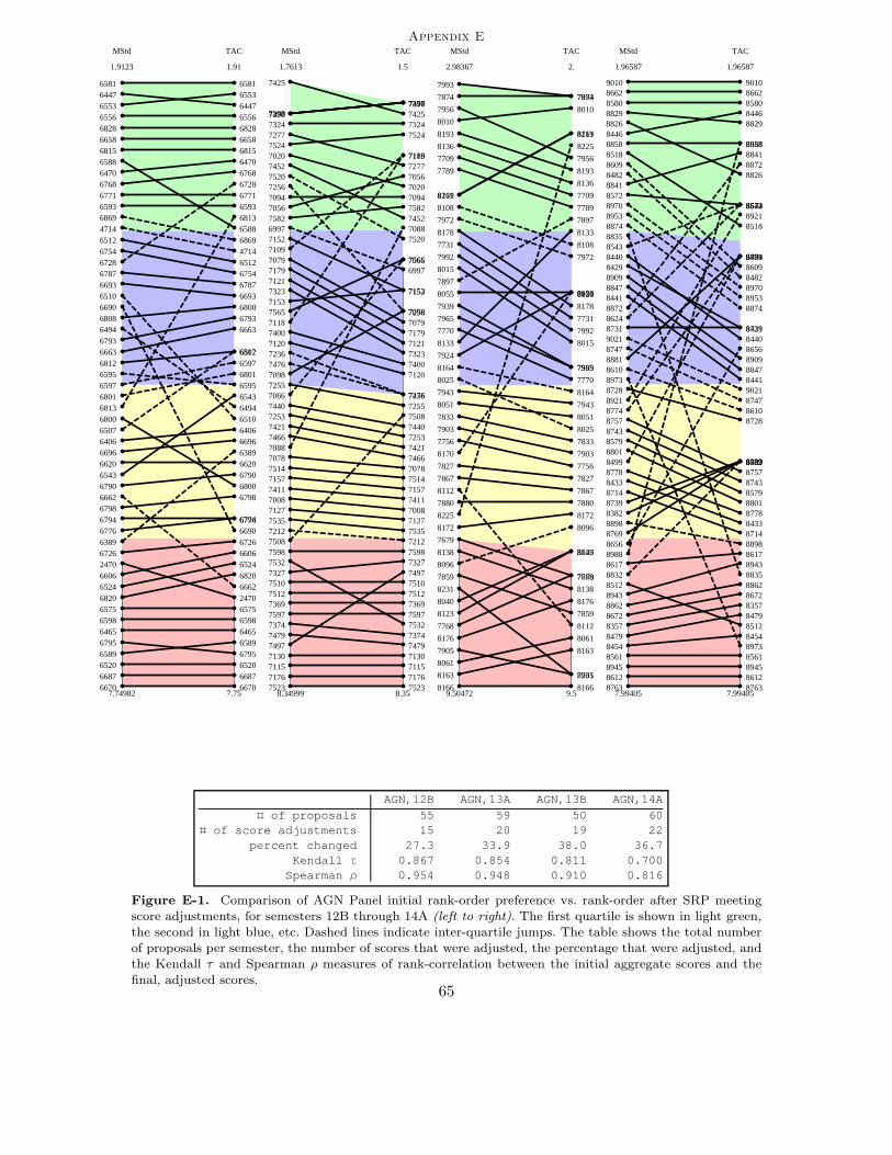
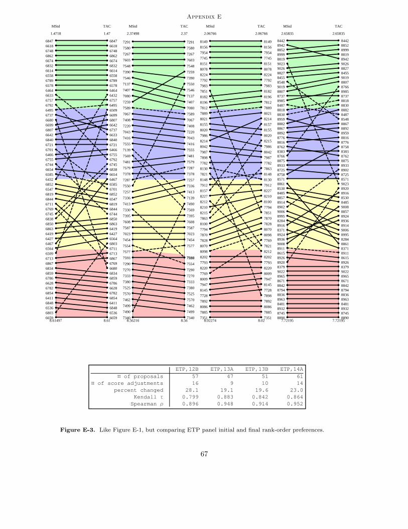
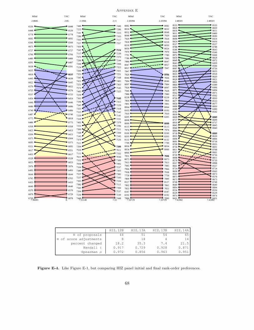
Figure E-1. Comparison of AGN Panel initial rank-order preference vs. rank-order after SRP meeting

score adjustments, for semesters 12B through 14A (left to right). The first quartile is shown in light green,the second in light blue, etc. Dashed lines indicate inter-quartile jumps. The table shows the total numberof proposals per semester, the number of scores that were adjusted, the percentage that were adjusted, andthe Kendall τ and Spearman ρ measures of rank-correlation between the initial aggregate scores and thefinal, adjusted scores.

65

Appendix E

6342

6417

6421

6431

6439

6441

6458

6489

6515

6518

6522

6548

6555

6560

6568

6571

6580

6601

6647

6650

6667

6668

6700

6707

6783

6799

6805

6816

6837

6853

6855

6865

6877

6342

6417

6421

6431

6439

6441

6458

6489

6515

6518

6522

6548

6555

6560

6568

6571

6580

6601

6647

6650

6667

6668

6700

6707

6783

6799

6805

6816

6837

6853

6855

6865

6877

8.46667

2.89947

8.47

2.9

MStd TAC

6401

6988

6990

6998

7006

7007

7034

7046

7063

7070

7071

7075

7076

7089

7140

7159

7160

7164

7166

7198

7210

7217

7224

7238

7268

7302

7313

7326

7366

7388

7392

7420

7434

7436

7447

7472

7474

7477

7480

7504

7515

7530

7538

7540

7547

7556

7567

7610

6401

6988

6990

6998

7006

7007

7034

7046

7063

7070

7071

7075

7076

7089

7140

7159

7160

7164

7166

7198

7210

7217

7224

7238

7268

7302

7313

7326

7366

7388

7392

7420

7434

7436

7447

7472

7474

7477

7480

7504

7515

7530

7538

7540

7547

7556

7567

7610

7.90915

1.77027

7.91

1.77

MStd TAC

7719

7729

7743

7754

7773

7787

7790

7823

7830

7855

7871

7922

7930

7931

7953

7973

7978

7994

7999

8004

8014

8026

8027

8030

8035

8060

8072

8104

8141

8162

8174

8175

8191

7719

7729

7743

7754

7773

7787

7790

7823

7830

7855

7871

7922

7930

7931

7953

7973

7978

7994

7999

8004

8014

8026

8027

8030

8035

8060

8072

8104

8141

8162

8174

8175

8191

8.32458

2.70189

8.32

2.7

MStd TAC

7950

8358

8392

8405

8423

84538465

8468

8483

8495

8498

8500

8507

8547

8552

8558

8559

8560

8591

8595

8613

8619

8622

8631

8633

8634

8663

8666

8680

8696

8700

8705

8715

8727

8738

8740

8744

8746

8753

87598761

8793

8798

8815

8817

8864

8879

8889

8934

8937

8950

8951

8979

89828989

8992

8994

9002

9003

7950

8358

8392

8405

8423

84538465

8468

8483

8495

8498

8500

8507

8547

8552

8558

8559

8560

8591

8595

8613

8619

8622

8631

8633

8634

8663

8666

8680

8696

8700

8705

8715

8727

8738

8740

8744

8746

8753

87598761

8793

8798

8815

8817

8864

8879

8889

8934

8937

8950

8951

8979

8982

8989

8992

8994

9002

9003

9.20168

2.38068

9.2

2.38068

MStd TAC

EGS,12B EGS,13A EGS,13B EGS,14A

ð of proposals 33 48 33 59ð of score adjustments 5 4 2 15

percent changed 15.2 8.3 6.1 25.4Kendall Τ 0.938 0.980 0.989 0.817Spearman Ρ 0.981 0.998 0.999 0.894

Figure E-2. Like Figure E-1, but comparing EGS panel initial and final rank-order preferences.

66

Appendix E

6411

64196427

6432

6464

6466

6467

6495

6509

6536

6547

6558

6564

6578

6585

6614

6618

6628

6633

6642

6654

6659

6674

66806699

6701

6711

6713

6721

6737

6744

6745

6748

6755

6757

6769

6782

6786

6789

6792

6803

6807

6819

6832

6834

6838

6840

6844

6847

6848

6850

6852

6854

6859

6862

6863

6867

6411

64196427

64326464

6466

6467

64956509

6536

6547

6558

6564

6578

6585

6614

6618

6628

6633

6642

6654

6659

6674

6680

6699

6701

67116713

6721

6737

6744

6745

6748

6755

6757

6769

6782

6786

6789

6792

6803

6807

6819

6832

6834

6838

6840

6844

6847

6848

6850

6852

6854

6859

6862

6863

6867

8.61497

1.4718

8.61

1.47

MStd TAC

7023

7043

7067

7080

7137

7139

7220

7257

7259

7267

7270

7287

7290

7291

7330

7333

7336

7340

7378

7380

7390

7395

7407

7408

7413

7416

7454

7462

7481

7490

7499

7525

7546

7548

7550

7554

7555

7569

7570

7577

7579

7580

7587

7589

7593

7603

7608

7023

7043

7067

7080

7137

7139

7220

7257

7259

7267

7270

7287

7290

7291

7330

7333

7336

7340

7378

7380

7390

7395

7407

7408

7413

7416

7454

7462

7481

7490

7499

7525

7546

7548

7550

7554

7555

7569

7570

7577

7579

7580

7587

7589

7593

7603

7608

8.56216

2.37498

8.56

2.37

MStd TAC

7351

7728

7745

7769

7782

7792

7793

7794

7812

7821

7828

7851

7863

7870

7885

7889

7892

7898

7912

7947

7954

7983

7986

7987

8009

8020

8021

8042

8070

8078

8086

8098

8100

8130

8145

8148

8149

8151

8155

8156

8157

8182

8196

8202

8210

8212

8214

8215

8220

8224

8227

8.02274

2.06766

8.02

2.06766

MStd TAC

8284

8371

8379

8383

8442

8455

8481

8485

8487

8530

8548

8571

8615

8671

8725

8737

8745

8758

8762

8766

8776

8794

8807

8816

8818

8819

8827

8830

8836

8842

8852

8857

8861

8867

8875

8882

8890

8892

8902

8911

8914

8916

8920

8924

8926

8932

8933

8936

8942

8959

8963

8965

8985

8995

8999

9006

9008

9019

9022

90239026

8284

8371

8379

8383

8442

8455

8481

8485

8487

8530

8548

8571

8615

8671

8725

8737

8745

8758

8762

8766

8776

8794

8807

8816

8818

8819

8827

8830

8836

8842

8852

8857

8861

8867

8875

8882

8890

8892

8902

8911

8914

89168920

8924

8926

8932

8933

8936

8942

8959

8963

8965

8985

8995

8999

9006

9008

9019

9022

9023

9026

7.72195

2.65835

7.72195

2.65835

MStd TAC

ETP,12B ETP,13A ETP,13B ETP,14A

ð of proposals 57 47 51 61ð of score adjustments 16 9 10 14

percent changed 28.1 19.1 19.6 23.0Kendall Τ 0.799 0.883 0.842 0.864Spearman Ρ 0.896 0.948 0.914 0.952

Figure E-3. Like Figure E-1, but comparing ETP panel initial and final rank-order preferences.

67

Appendix E

5976

6358

6375

6423

6433

6445

6446

6448

6453

6454

6480

6486

6487

6493

6504

6526

6528

6537

6551

6566

6570

6576

6591

6617

6635

6638

6640

6644

6653

6675

6686

6692

6695

6706

6725

6727

6729

6740

6765

6775

6778

6818

6822

6878

5976

6358

6375

6423

6433

6445

6446

6448

6453

6454

6480

6486

6487

6493

6504

6526

6528

6537

6551

6566

6570

6576

6591

6617

6635

6638

6640

6644

6653

6675

6686

6692

6695

6706

6725

6727

6729

6740

6765

6775

6778

6818

6822

68787.96001

2.8845

8.

2.85

MStd TAC

7036

7104

7111

7117

7141

7145

7154

7163

7168

7196

7204

7223

7229

7230

7231

7237

7239

7244

7251

7266

7286

7296

7300

7303

7315

7318

7325

7332

7343

7345

7353

7363

7370

7379

7382

7389

7394

7430

7431

7446

7448

7483

7492

7511

7526

7537

7542

7545

7557

7574

7611 7036

7104

7111

7117

7141

7145

7154

7163

7168

7196

7204

7223

7229

7230

7231

7237

7239

7244

7251

7266

7286

7296

7300

7303

7315

7318

7325

7332

7343

7345

7353

7363

7370

7379

7382

7389

7394

7430

7431

7446

7448

7483

7492

7511

7526

7537

7542

7545

7557

7574

7611

7.55148

2.1066

7.55

2.11

MStd TAC

7758

77807791

7799

7800

7818

7822

7826

7831

7847

7862

7864

7886

7890

7891

7910

7913

7928

7929

7938

7946

7966

7970

7974

7980

7984

7985

8008

80248032

8046

8047

8048

8050

80548056

8057

8064

8066

8073

8082

8097

8099

8103

8115

8127

8132

8160

81878192

8203

8205

8218

8228

7758

7780

7791

7799

7800

7818

7822

7826

7831

7847

7862

7864

7886

7890

7891

7910

7913

7928

7929

7938

7946

7966

7970

7974

7980

7984

7985

8008

8024

8032

8046

8047

8048

8050

8054

8056

8057

8064

8066

8073

8082

8097

8099

8103

8115

8127

8132

8160

81878192

8203

8205

8218

8228

7.50729

2.20394

7.50729

2.20394

MStd TAC

8346

8389

8400

8416

8424

8431

8444

8459

8490

8494

8496

8513

8527

8529

8533

8542

8556

8557

8562

8563

8578

8584

8620

8630

8640

8643

8655

8661

8673

8677

8690

8691

8699

8707

8708

8717

8718

8720

8724

8726

8756

8768

8788

8811

8820

8821

8828

8845

8849

8850

8866

8873

8884

8894

8910

8918

8935

8939

8940

8971

8972

8974

8997

8998

9011

8346

8389

8400

84168424

8431

8444

8459

8490

84948496

8513

8527

8529

8533

8542

8556

8557

8562

8563

8578

8584

8620

8630

8640

8643

8655

8661

8673

8677

8690

8691

86998707

8708

8717

8718

8720

8724

8726

8756

8768

8788

8811

8820

8821

8828

8845

8849

8850

8866

8873

8884

8894

8910

8918

8935

8939

8940

8971

8972

8974

8997

8998

9011

7.42082

2.48501

7.42082

2.48501

MStd TAC

HIZ,12B HIZ,13A HIZ,13B HIZ,14A

ð of proposals 44 51 54 65ð of score adjustments 8 18 4 14

percent changed 18.2 35.3 7.4 21.5Kendall Τ 0.917 0.729 0.928 0.871Spearman Ρ 0.972 0.856 0.963 0.951

Figure E-4. Like Figure E-1, but comparing HIZ panel initial and final rank-order preferences.

68

Appendix E

6377

6404

6418

6425

6430

6434

6438

6463

6482

6517

6584

6592

6611

6613

6619

6626

6630

6648

6673

6676

6717

6759

6760

6770

6823

6826

6827

6833

6377

6404

6418

6425

6430

6434

6438

6463

6482

6517

6584

6592

6611

6613

6619

6626

6630

6648

6673

6676

6717

6759

6760

6770

6823

6826

6827

6833

7.31157

3.67871

7.31

3.68

MStd TAC

6708

6983

7013

7017

7030

7058

7068

7082

70837110

7116

7123

7155

7167

7170

7171

7186

7225

7233

7234

7248

7271

7272

7281

7288

7295

7298

7299

7301

7322

7328

7337

73417346

7362

7371

7381

7393

7401

7403

74047422

7442

7449

7451

7458

7461

74657468

7484

7485

7491

7493

7495

7507

7519

7522

7528

7543

7578

6708

6983

7013

7017

7030

7058

7068

7082

70837110

71167123

7155

7167

7170

7171

7186

7225

7233

7234

7248

7271

7272

7281

7288

7295

7298

7299

7301

7322

7328

7337

7341

7346

7362

7371

7381

7393

7401

7403

7404

7422

7442

7449

7451

7458

7461

74657468

7484

7485

7491

7493

7495

7507

7519

7522

7528

7543

7578

7.99198

2.45612

7.99

2.46

MStd TAC

6895

7765

7795

7796

7807

7813

7819

7820

7832

7844

7848

7872

7881

7901

7917

7949

7952

7975

7995

8001

8003

8019

8038

8039

8043

8083

8085

8088

8091

8095

8106

8109

8128

8137

8142

8194

8217

8221

8222

8226

8229

8236

6895

7765

7795

7796

7807

7813

7819

7820

7832

7844

7848

7872

7881

7901

7917

7949

7952

7975

7995

8001

8003

8019

8038

8039

8043

8083

8085

8088

8091

8095

8106

8109

8128

8137

8142

8194

8217

8221

8222

8226

8229

8236

8.05029

2.50949

8.05

2.51

MStd TAC

8380

8436

8448

8456

8462

8464

84718486

8504

8505

8581

8583

8596

8600

8602

8606

8611

8623

8627

8637

8647

8648

8651

8659

8664

8678

8685

8701

8702

8703

8710

8734

8741

8742

87558764

8765

87708773

8800

8803

8823

8838

8839

8855

8876

8883

8886

8887

8888

8891

8904

8922

8923

8930

8938

8962

8980

9005

9013

9020

8.22937

2.35615

8.23

2.36

MStd TAC

ISM,12B ISM,13A ISM,13B ISM,14A

ð of proposals 28 60 42 61ð of score adjustments 7 9 6 5

percent changed 25.0 15.0 14.3 8.2Kendall Τ 0.889 0.950 0.887 0.879Spearman Ρ 0.968 0.991 0.946 0.916

Figure E-5. Like Figure E-1, but comparing ISM panel initial and final rank-order preferences.

69

Appendix E

6413

6416

6452

6484

6501

6511

6523

6530

6532

6541

6559

6562

6573

6577

6582

6590

6610

6623

6624

6646

6694

6739

6741

6785

6821

6836

6839

6849

6413

6416

6452

6484

6501

6511

6523

6530

6532

6541

6559

6562

6573

6577

6582

6590

6610

6623

6624

6646

6694

6739

6741

6785

6821

6836

6839

6849

9.17861

2.8066

9.18

2.56

MStd TAC

7033

7045

7060

7095

7106

7114

7119

7126

7129

7178

7183

7199

7205

7209

7213

7214

7228

7240

7245

7276

7279

7292

7293

7314

7334

7338

7347

7377

7387

7418

7424

7426

7427

7432

7433

7489

7516

7518

7563

7566

7573

7581

7601

7033

7045

7060

7095

7106

7114

7119

7126

7129

7178

7183

7199

7205

7209

7213

7214

7228

7240

7245

7276

7279

7292

7293

7314

7334

7338

7347

7377

7387

7418

7424

7426

7427

7432

7433

7489

7516

7518

7563

7566

7573

7581

7601

7.5521

3.15706

7.61

2.04

MStd TAC

7714

7771

7779

7786

7810

7815

7835

7846

7849

7852

7868

7878

7879

7884

7887

7894

7923

7948

7991

7996

8058

8059

8062

8071

8102

8116

8122

8129

8144

8159

8165

8197

8216

7714

7771

7779

7786

7810

7815

7835

7846

7849

7852

7868

7878

7879

7884

7887

7894

7923

7948

7991

7996

8058

8059

8062

8071

8102

8116

8122

8129

8144

8159

8165

8197

8216

7.65997

2.7323

7.66

2.73

MStd TAC

8381

8409

8410

8412

8414

8421

8434

8435

8447

8469

8473

8474

8510

8522

8523

8524

8532

8535

8546

8549

8550

8565

8601

8628

8646

8665

8669

8674

8675

8723

8806

8824

8825

8837

8844

8846

8863

8869

8878

8897

8905

8906

8955

8958

8996

9004

8381

8409

8410

8412

8414

8421

8434

8435

8447

8469

8473

8474

8510

8522

8523

8524

8532

8535

8546

8549

8550

8565

8601

8628

8646

8665

8669

8674

8675

8723

8806

8824

8825

8837

8844

8846

8863

8869

8878

8897

8905

8906

8955

8958

8996

9004

7.7146

2.71469

7.71

2.71

MStd TAC

NGA,12B NGA,13A NGA,13B NGA,14A

ð of proposals 28 43 33 46ð of score adjustments 11 42 6 6

percent changed 39.3 97.7 18.2 13.0Kendall Τ 0.796 0.491 0.871 0.953Spearman Ρ 0.910 0.668 0.948 0.988

Figure E-6. Like Figure E-1, but comparing NGA panel initial and final rank-order preferences.

70

Appendix E

6380

6415

64246457

6468

6472

6497

6498

6499

6502

6505

6519

6521

6529

6533

6542

65446554

6563

6587

6594

6596

6600

6605

6612

6627

6631

6636

664566526679

6681

6682

66856689

6691

6697

6709

6715

6722

6723

6731

6742

6746

6747

6753

6764

6784

6809

6835

6858

6861

6864

6868

6380

6415

64246457

6468

6472

6497

6498

6499

6502

6505

6519

6521

6529

6533

6542

6544

6554

6563

6587

6594

6596

6600

6605

6612

6627

6631

6636

6645

66526679

6681

6682

6685

6689

6691

6697

6709

6715

6722

6723

6731

6742

6746

6747

6753

6764

6784

6809

6835

6858

6861

6864

6868

8.25841

2.74157

8.26

2.74

MStd TAC

6975

7004

7010

7024

7065

7069

7087

7099

7108

7112

7125

7132

7135

7146

7149

7158

7173

7180

7197

7203

7211

7216

7221

7249

7252

7254

7258

7261

7289

7304

7309

7358

7365

7367

7368

7386

7391

7396

7405

7409

7412

7435

7437

7443

7450

7457

7459

7460

7464

7467

7498

7500

7501

7502

7509

7521

7531

7551

7552

7553

7584

7585

7588

7602

6975

7004

7010

7024

7065

7069

7087

7099

7108

7112

7125

7132

71357146

7149

71587173

7180

7197

7203

7211

7216

7221

7249

7252

7254

7258

7261

7289

7304

7309

7358

7365

7367

7368

7386

7391

7396

7405

7409

7412

7435

7437

7443

7450

7457

7459

7460

7464

7467

7498

750075017502

7509

7521

75317551

7552

7553

7584

7585

7588

7602

7.96979

1.84243

7.97

1.84

MStd TAC

7645

7715

7717

7742

7746

7755

7760

7762

7772

7775

7778

7857

7873

7876

7893

7896

7900

7908

7909

7932

7940

7942

7957

7962

7963

7969

7989

8005

8013

8017

8028

8033

8034

8045

8052

8084

8089

8090

8150

8153

8167

8173

8183

8198

8207

7645

7715

7717

7742

7746

7755

7760

7762

7772

7775

7778

7857

7873

7876

7893

7896

7900

7908

7909

7932

7940

7942

7957

7962

7963

7969

7989

8005

8013

8017

8028

8033

8034

8045

8052

8084

8089

8090

8150

8153

8167

8173

8183

8198

8207

8.13459

2.77213

8.13

2.77213

MStd TAC

6579

8356

8376

8403

8437

8458

8477

8478

8492

8501

8519

8541

8569

8582

8585

8588

8590

8592

8597

8603

8604

8607

8618

8621

8626

8635

8638

8645

8653

8657

8676

8688

8693

86978704

8722

8729

8730

8748

8789

8797

8805

8822

8831

8833

8854

8865

8871

8885

8899

8903

8912

8927

8929

8941

8949

8956

8961

8977

8991

9015

6579

8356

8376

8403

8437

8458

8477

8478

8492

8501

8519

8541

8569

8582

85858588

8590

8592

8597

8603

8604

8607

8618

8621

8626

8635

8638

8645

8653

8657

8676

8688

8693

86978704

8722

8729

8730

8748

8789

8797

8805

8822

8831

8833

8854

8865

8871

8885

8899

8903

8912

8927

8929

8941

8949

8956

8961

8977

8991

9015

7.38227

2.73355

7.38227

2.5

MStd TAC

SFM,12B SFM,13A SFM,13B SFM,14A

ð of proposals 54 64 45 61ð of score adjustments 21 20 13 7

percent changed 38.9 31.2 28.9 11.5Kendall Τ 0.804 0.926 0.857 0.910Spearman Ρ 0.903 0.986 0.954 0.964

Figure E-7. Like Figure E-1, but comparing SFM panel initial and final rank-order preferences.

71

Appendix E

6357

6395

6422

6451

6455

6481

6514

6552

6567

6629

6639

6678

6719

6749

6779

6791

6802

6804

6817

6846

6871

6874

6357

6395

6422

6451

6455

6481

6514

6552

6567

6629

6639

6678

6719

6749

6779

6791

6802

6804

6817

6846

6871

6874

7.56198

2.43282

7.56

2.43

MStd TAC

6461

6492

6999

7031

7057

7061

7084

7085

7093

7122

7206

7227

7241

7246

7307

7311

7335

7348

7355

7357

7359

7361

7364

7375

7384

7406

7438

7439

7455

7456

7469

7471

7513

7564

7568

7595

7599

7600

7606

7607

6461

6492

6999

7031

7057

7061

7084

7085

7093

7122

7206

7227

7241

7246

7307

7311

7335

7348

7355

7357

7359

7361

7364

7375

7384

7406

7438

7439

7455

7456

7469

7471

7513

7564

7568

7595

7599

7600

7606

7607

7.73063

2.91602

7.73

2.92

MStd TAC

6918

7747

7749

7763

7767

7784

7808

7839

7865

7882

7895

7918

7941

7988

7998

8000

8006

8011

8012

8036

8053

8065

8074

8077

8079

8081

8087

8093

8110

8118

8131

8134

8139

8181

8184

8185

8200

8201

8209

8223

8230

8232

8233

6918

7747

7749

7763

7767

7784

7808

7839

7865

7882

7895

7918

7941

7988

7998

8000

8006

8011

8012

8036

8053

8065

8074

8077

8079

8081

8087

8093

8110

8118

8131

8134

8139

8181

8184

8185

8200

8201

8209

8223

8230

8232

82339.62126

2.3081

9.62

2.31

MStd TAC

8452

8467

8489

8497

8506

8515

8516

8517

8539

8589

8599

8608

8614

8629

8658

8660

8712

8760

8781

8787

8808

8843

8895

8907

8925

8931

8944

8947

8969

8976

8983

9025

8452

8467

8489

8497

8506

8515

8516

8517

8539

8589

8599

8608

8614

8629

8658

8660

8712

8760

8781

8787

8808

8843

8895

8907

8925

8931

8944

8947

8969

8976

8983

90258.02685

2.69349

8.03

2.69

MStd TAC

SSP,12B SSP,13A SSP,13B SSP,14A

ð of proposals 22 40 43 32ð of score adjustments 5 10 5 0

percent changed 22.7 25.0 11.6 0.0Kendall Τ 0.879 0.871 0.901 1.000Spearman Ρ 0.957 0.940 0.944 1.000

Figure E-8. Like Figure E-1, but comparing SSP panel initial and final rank-order preferences.

72

Appendix F

0 2 4 6 8 100.0

0.2

0.4

0.6

0.8

1.0

Score, s

Frac

tion

Adj. Linearized Score CDFs, Cycle 12B

0 2 4 6 8 100.0

0.2

0.4

0.6

0.8

1.0

Score, s

Frac

tion

Adj. Linearized Score CDFs, Cycle 13A

0 2 4 6 8 100.0

0.2

0.4

0.6

0.8

1.0

Score, s

Frac

tion

Adj. Linearized Score CDFs, Cycle 13B

0 2 4 6 8 100.0

0.2

0.4

0.6

0.8

1.0

Score, s

Frac

tion

Adj. Linearized Score CDFs, Cycle 14A

Figure F-1. These plots show the cumulative distributions of adjusted, linearized SRP aggregate scores,by instrument. GBT proposal scores are shown in blue, VLA scores in green, and VLBA/HSA scores in red.

73

Appendix F

Adjusted, Linearized Score CDFs, AGN Panel

0 2 4 6 8 10

0.0

0.2

0.4

0.6

0.8

1.0

12B, AGN

0 2 4 6 8 10

0.0

0.2

0.4

0.6

0.8

1.0

13A, AGN

0 2 4 6 8 10

0.0

0.2

0.4

0.6

0.8

1.0

13B, AGN

0 2 4 6 8 10

0.0

0.2

0.4

0.6

0.8

1.0

14A, AGN

Adjusted, Linearized Score CDFs, EGS Panel

0 2 4 6 8 10

0.0

0.2

0.4

0.6

0.8

1.0

12B, EGS

0 2 4 6 8 10

0.0

0.2

0.4

0.6

0.8

1.0

13A, EGS

0 2 4 6 8 10

0.0

0.2

0.4

0.6

0.8

1.0

13B, EGS

0 2 4 6 8 10

0.0

0.2

0.4

0.6

0.8

1.0

14A, EGS

Figure F-2. The cumulative distributions of adjusted, linearized SRP aggregate scores, by instrument, forthe AGN and EGS panls. (Continued on next page.)

74

Appendix F

Adjusted, Linearized Score CDFs, ETP Panel

0 2 4 6 8 10

0.0

0.2

0.4

0.6

0.8

1.0

12B, ETP

0 2 4 6 8 10

0.0

0.2

0.4

0.6

0.8

1.0

13A, ETP

0 2 4 6 8 10

0.0

0.2

0.4

0.6

0.8

1.0

13B, ETP

0 2 4 6 8 10

0.0

0.2

0.4

0.6

0.8

1.0

14A, ETP

Adjusted, Linearized Score CDFs, HIZ Panel

0 2 4 6 8 10

0.0

0.2

0.4

0.6

0.8

1.0

12B, HIZ

0 2 4 6 8 10

0.0

0.2

0.4

0.6

0.8

1.0

13A, HIZ

0 2 4 6 8 10

0.0

0.2

0.4

0.6

0.8

1.0

13B, HIZ

0 2 4 6 8 10

0.0

0.2

0.4

0.6

0.8

1.0

14A, HIZ

Figure F-2 (Continued). The cumulative distributions of adjusted, linearized SRP aggregate scores, byinstrument, for the ETP and HIZ panels. (Continued on next page.)

75

Appendix F

Adjusted, Linearized Score CDFs, ISM Panel

0 2 4 6 8 10

0.0

0.2

0.4

0.6

0.8

1.0

12B, ISM

0 2 4 6 8 10

0.0

0.2

0.4

0.6

0.8

1.0

13A, ISM

0 2 4 6 8 10

0.0

0.2

0.4

0.6

0.8

1.0

13B, ISM

0 2 4 6 8 10

0.0

0.2

0.4

0.6

0.8

1.0

14A, ISM

Adjusted, Linearized Score CDFs, NGA Panel

0 2 4 6 8 10

0.0

0.2

0.4

0.6

0.8

1.0

12B, NGA

0 2 4 6 8 10

0.0

0.2

0.4

0.6

0.8

1.0

13A, NGA

0 2 4 6 8 10

0.0

0.2

0.4

0.6

0.8

1.0

13B, NGA

0 2 4 6 8 10

0.0

0.2

0.4

0.6

0.8

1.0

14A, NGA

Figure F-2 (Continued). The cumulative distributions of adjusted, linearized SRP aggregate scores, byinstrument, for the ISM and NGA panels. (Continued on next page.)

76

Appendix F

Adjusted, Linearized Score CDFs, SFM Panel

0 2 4 6 8 10

0.0

0.2

0.4

0.6

0.8

1.0

12B, SFM

0 2 4 6 8 10

0.0

0.2

0.4

0.6

0.8

1.0

13A, SFM

0 2 4 6 8 10

0.0

0.2

0.4

0.6

0.8

1.0

13B, SFM

0 2 4 6 8 10

0.0

0.2

0.4

0.6

0.8

1.0

14A, SFM

Adjusted, Linearized Score CDFs, SSP Panel

0 2 4 6 8 10

0.0

0.2

0.4

0.6

0.8

1.0

12B, SSP

0 2 4 6 8 10

0.0

0.2

0.4

0.6

0.8

1.0

13A, SSP

0 2 4 6 8 10

0.0

0.2

0.4

0.6

0.8

1.0

13B, SSP

0 2 4 6 8 10

0.0

0.2

0.4

0.6

0.8

1.0

14A, SSP

Figure F-2 (Continued). The cumulative distributions of adjusted, linearized SRP aggregate scores, byinstrument, for the SFM and SSP panels. (Continued on next page.)

77

Appendix F

0 2 4 6 8 100.0

0.2

0.4

0.6

0.8

1.0

12B, ETP Pulsar Proposal PDFs

0 2 4 6 8 100.0

0.2

0.4

0.6

0.8

1.0

12B, ETP Pulsar Proposal CDFs

0 2 4 6 8 100.0

0.2

0.4

0.6

0.8

1.0

13A, ETP Pulsar Proposal PDFs

0 2 4 6 8 100.0

0.2

0.4

0.6

0.8

1.0

13A, ETP Pulsar Proposal CDFs

0 2 4 6 8 100.0

0.2

0.4

0.6

0.8

1.0

13B, ETP Pulsar Proposal PDFs

0 2 4 6 8 100.0

0.2

0.4

0.6

0.8

1.0

13B, ETP Pulsar Proposal CDFs

0 2 4 6 8 100.00

0.05

0.10

0.15

0.20

0.25

0.30

14A, ETP Pulsar Proposal PDFs

0 2 4 6 8 100.0

0.2

0.4

0.6

0.8

1.0

14A, ETP Pulsar Proposal CDFs

Figure F-3. Comparison of linearized, adjusted score distributions for ETP pulsar proposals, by instru-ment. GBT proposal scores are shown in blue, VLA scores in green, and VLBA/HSA scores in red. Comparewith Figure F-4.

78

Appendix F

0 2 4 6 8 100.0

0.2

0.4

0.6

0.8

1.0

12B, ETP Triggered Proposal PDFs

0 2 4 6 8 100.0

0.2

0.4

0.6

0.8

1.0

12B, ETP Triggered Proposal CDFs

0 2 4 6 8 100.00

0.05

0.10

0.15

0.20

0.25

0.30

13A, ETP Triggered Proposal PDFs

0 2 4 6 8 100.0

0.2

0.4

0.6

0.8

1.0

13A, ETP Triggered Proposal CDFs

0 2 4 6 8 100.0

0.2

0.4

0.6

0.8

1.0

13B, ETP Triggered Proposal PDFs

0 2 4 6 8 100.0

0.2

0.4

0.6

0.8

1.0

13B, ETP Triggered Proposal CDFs

0 2 4 6 8 100.0

0.1

0.2

0.3

0.4

0.5

14A, ETP Triggered Proposal PDFs

0 2 4 6 8 100.0

0.2

0.4

0.6

0.8

1.0

14A, ETP Triggered Proposal CDFs

Figure F-4. Comparison of linearized, adjusted score distributions for ETP triggered proposals, by in-strument. GBT proposal scores are shown in blue, VLA scores in green, and VLBA/HSA scores in red.Compare with Figure F-3.

79

0.3 0.4 0.5 0.6 0.7 0.8

1

2

3

4

5

6

AGN,12B 0.544 0.621 0.598 0.681 0.579 0.555AGN,13A 0.638 0.672 0.700 0.549 0.670 0.670AGN,13B 0.564 0.699 0.691 0.647 0.494 0.665AGN,14A 0.550 0.535 0.672 0.568 0.557EGS,12B 0.493 0.638 0.680 0.613 0.660 0.520EGS,13A 0.594 0.669 0.685 0.633 0.625 0.507EGS,13B 0.684 0.616 0.563 0.671 0.520 0.640EGS,14A 0.576 0.565 0.617 0.629 0.632 0.586ETP,12B 0.574 0.571 0.585 0.594 0.705ETP,13A 0.683 0.597 0.632 0.634 0.740ETP,13B 0.513 0.575 0.702 0.575 0.660 0.599ETP,14A 0.582 0.676 0.600 0.589 0.605 0.608HIZ,12B 0.683 0.666 0.563 0.561 0.560 0.578HIZ,13A 0.561 0.633 0.600 0.526 0.565 0.512HIZ,13B 0.583 0.606 0.682 0.577 0.629 0.250HIZ,14A 0.587 0.691 0.642 0.652 0.579 0.552ISM,12B 0.583 0.497 0.583 0.376 0.556 0.681ISM,13A 0.617 0.609 0.661 0.620 0.636 0.638ISM,13B 0.585 0.545 0.626 0.583 0.617 0.456ISM,14A 0.579 0.570 0.458 0.579 0.622 0.575NGA,12B 0.544 0.577 0.740 0.659 0.686 0.624NGA,13A 0.610 0.682 0.580 0.603 0.553 0.264NGA,13B 0.464 0.631 0.606 0.742 0.721 0.610NGA,14A 0.560 0.600 0.587 0.581 0.552 0.588SFM,12B 0.669 0.706 0.586 0.617 0.540SFM,13A 0.702 0.622 0.674 0.688 0.673 0.602SFM,13B 0.673 0.545 0.639 0.641 0.533 0.688SFM,14A 0.511 0.608 0.594 0.518 0.585 0.650SSP,12B 0.665 0.605 0.639 0.773 0.611 0.489SSP,13A 0.616 0.651 0.813 0.617 0.525 0.634SSP,13B 0.783 0.712 0.488 0.618 0.440 0.539SSP,14A 0.598 0.725 0.625 0.566 0.605

Figure F-5. The table above shows modified Borda counts for each reviewer in each of the eight SRPs,

for semesters 12B, 13A, 13B, and 14A. This is for comparison of individual reviewers’ preliminary scoreswith the SRP average, normalized preliminary scores. These correspond to the Qprelim values in Table 1,Line 1 of Neill Reid’s Memorandum [21]. (We cannot compute the Qfinal scores, as he has done, becauseour panelists do not individually submit revised proposal scores; but rather they agree by acclamation ona consensus score for each proposal.) Also shown is a smooth histogram of the entire list of Qinitial values.The mean value, 0.605 ± 0.075, is very close to that of [21].

80


Recommended