313 MARCH 2008 AMERICAN METEOROLOGICAL SOCIETY | THE COSMIC/FORMOSAT-3 MISSION THE COSMIC/FORMOSAT-3 MISSION Early Results Early Results BY R. A. ANTHES, P. A. BERNHARDT , Y. CHEN, L. CUCURULL, K. F. DYMOND, D. ECTOR, S. B. HEALY , S.-P. HO, D. C. HUNT , Y.-H. KUO, H. LIU, K. MANNING, C. MCCORMICK, T. K. MEEHAN, W. J. RANDEL, C. ROCKEN, W. S. SCHREINER, S. V. SOKOLOVSKIY, S. SYNDERGAARD, D. C. T HOMPSON, K. E. T RENBERTH, T.-K. WEE, N. L. Y EN, AND Z. ZENG The COSMIC radio occultation mission represents a revolution in atmospheric sounding from space, with precise, accurate, and all-weather global observations useful for weather, climate, and space weather research and operations. 1 For simplicity we will refer to the mission as COSMIC in this paper. T he global positioning system (GPS) radio-occultation (RO) limb-sounding technique for sounding Earth’s atmosphere was demonstrated by the proof-of-concept GPS Meteorology (GPS/MET) experiment in 1995–97 (Ware et al. 1996). Following GPS/MET, additional missions, that is, the Challenging Minisatellite Payload (CHAMP; Wickert et al. 2001) and the Satellite de Aplicaciones Cientificas-C (SAC-C; Hajj et al. 2004), have confirmed the potential of RO sounding of the ionosphere, stratosphere, and troposphere. At 0140 UTC 15 April 2006, six microsatellites were launched into a circular, 72° inclination orbit at an altitude of 512 km from Vandenberg Air Force Base, California (Cheng et al. 2006). The mission is a collaborative project of the National Space Organization (NSPO) in Taiwan and the University Corporation for Atmospheric Research (UCAR) in the United States. The mission is called the Constellation Observing System for Meteorology, Ionosphere, and Climate (COSMIC) in the United States and the Formosa Satellite Mission 3 (FORMOSAT-3) in Taiwan. 1 All satellites began delivering useful data within days FIG. 1. Schematic diagram illustrating radio occultation of GPS signals. [Figure courtesy of NSPO.]
Transcript
313MARCH 2008AMERICAN METEOROLOGICAL SOCIETY |
THE COSMIC/FORMOSAT-3 MISSIONTHE COSMIC/FORMOSAT-3 MISSION Early Results Early Results
BY R. A. ANTHES, P. A. BERNHARDT, Y. CHEN, L. CUCURULL, K. F. DYMOND, D. ECTOR, S. B. HEALY, S.-P. HO, D. C. HUNT, Y.-H. KUO, H. LIU, K. MANNING, C. MCCORMICK, T. K. MEEHAN, W. J. RANDEL, C. ROCKEN, W. S. SCHREINER, S. V. SOKOLOVSKIY, S. SYNDERGAARD, D. C. THOMPSON, K. E. TRENBERTH, T.-K. WEE, N. L. YEN, AND Z. ZENG
The COSMIC radio occultation mission represents a revolution in atmospheric sounding from space, with precise, accurate, and all-weather global observations useful for weather,
climate, and space weather research and operations.
1 For simplicity we will refer to the mission as COSMIC in this paper.
T he global positioning system (GPS) radio-occultation (RO) limb-sounding technique
for sounding Earth’s atmosphere was demonstrated by the proof-of-concept GPS
Meteorology (GPS/MET) experiment in 1995–97 (Ware et al. 1996). Following
GPS/MET, additional missions, that is, the Challenging Minisatellite Payload (CHAMP;
Wickert et al. 2001) and the Satellite de Aplicaciones Cientificas-C (SAC-C; Hajj et al.
2004), have confirmed the potential of RO sounding of the ionosphere, stratosphere, and
troposphere.
At 0140 UTC 15 April 2006, six microsatellites were launched into a circular, 72°
inclination orbit at an altitude of 512 km from Vandenberg Air Force Base, California
(Cheng et al. 2006). The mission is a collaborative project of the National Space Organization
(NSPO) in Taiwan and the University Corporation for Atmospheric Research (UCAR) in the
United States. The mission is called the Constellation Observing System for Meteorology,
Ionosphere, and Climate (COSMIC) in the United States and the Formosa Satellite Mission
3 (FORMOSAT-3) in Taiwan.1 All satellites began delivering useful data within days
FIG. 1. Schematic diagram illustrating radio occultation of GPS signals. [Figure courtesy of NSPO.]
314 MARCH 2008|
after the launch (Anthes 2006). This paper sum-
marizes the mission and the early scientific results,
with emphasis on the radio-occultation part of the
mission.
The primary payload of each COSMIC satellite is
a GPS radio-occultation receiver developed by the
National Aeronautics and Space Administration’s
(NASA’s) Jet Propulsion Laboratory (JPL). By
measuring the phase delay of radio waves from
GPS satellites as they are occulted by the Earth’s
atmosphere (Fig. 1), accurate and precise vertical
profiles of the bending angles of radio wave trajec-
tories are obtained in the ionosphere, stratosphere,
and troposphere. From the bending angles, profiles
of atmospheric refractivity are obtained. The
procedures used to obtain stratospheric and tropo-
spheric bending angle and refractivity profiles from
the raw phase and amplitude data for the COSMIC
mission are described by Kuo et al. (2004).
The radio-occultation method for obtaining atmo-
spheric soundings is summarized by Kursinski et al.
(1997) and in a special issue of Terrestrial, Atmospheric
and Oceanic Sciences (2000, Vol. 1, hereafter TAO).
TAO also describes the RO method; the application of
RO to weather, climate, and ionospheric research; and
the COSMIC mission. The refractivity N is a function
of temperature (T; K), pressure (p; hPa), water vapor
pressure (e; hPa), and electron density (ne; number of
electrons per cubic meter),
(1)
In (1), ƒ is the frequency of the GPS carrier signal
(Hz).
The refractivity profiles can be used to derive
profiles of electron density in the ionosphere,
temperature in the stratosphere, and temperature and
water vapor in the troposphere. The RO technique
and its history, which starts with the exploration
of Mars in the 1960s and was later applied to other
planets, are described by Yunck et al. (2000).
The COSMIC satellites also carry two other
payloads, which were developed by the Naval Research
Laboratory (NRL). The tiny ionospheric photometer
(TIP) monitors the intensity of emissions that result
from the recombination of oxygen ions with electrons
at ionospheric altitudes; the observed intensities can
be converted to electron density in the ionosphere.
The TIP measurements can monitor the electron
density depletions associated with ionospheric
bubbles that are frequently associated with radio
frequency scintillation. The nadir-pointing coherent
electromagnetic radio tomography (CERTO) tri-band
beacon (TBB) permits ionospheric observations
by measuring the phase differences at two or three
frequencies using ground-based receivers. Data
from the TBB receivers can be used to retrieve the
satellite-to-ground total electron content, to allow for
high-resolution tomography of the electron density
distribution, and to monitor phase and amplitude
scintillations induced in radio waves propagating
through the ionosphere. Together with the RO
observations, these instruments will contribute
observations of electron density of unprecedented
horizontal and vertical resolution to the operational
and research space weather communities.
While the primary scientific goal of COSMIC is
to demonstrate the value of near-real-time (NRT)
RO observations in operational numerical weather
prediction (NWP), some interesting scientific results
from COSMIC that are relevant for climate and other
atmospheric studies have already been obtained. This
paper summaries some of these results and also serves
to inform the scientific community about the avail-
ability of COSMIC data for research and operations.
The observations may be obtained free of charge
upon registration on the Web site of the Taiwan
AFFILIATIONS: ANTHES, ECTOR, HUNT, KUO, ROCKEN, SCHREINER, SOKOLOVSKIY, SYNDERGAARD, WEE, AND ZENG—University Corporation for Atmospheric Research, Boulder, Colorado; BERNHARDT AND DYMOND—Naval Research Laboratory, Washington, D.C.; CHEN, LIU, MANNING, RANDEL, AND TRENBERTH—National Center for Atmospher-ic Research, Boulder, Colorado; CUCURULL—University Corporation for Atmospheric Research, Boulder, Colorado, and Joint Center for Satellite Data Assimilation, Washington, D.C.; HO—University Corporation for Atmospheric Research, and National Center for Atmospheric Research, Boulder, Colorado; HEALY—European Cen-tre for Medium-Range Weather Forecasts, Reading, United King-dom; MCCORMICK—Broad Reach Engineering, Golden, Colorado;
MEEHAN—Jet Propulsion Laboratory, Pasadena, California; THOMPSON—Utah State University, Logan, Utah; YEN—Na-tional Space Organization, Hsin-Chu, TaiwanCORRESPONDING AUTHOR: Ying-Hwa Kuo, UCAR, P.O. Box 3000, Boulder, CO 80307E-mail: [email protected]
The abstract for this article can be found in this issue, following the table of contents.DOI:10.1175/BAMS-89-3-313
(at http://tacc.cwb.gov.tw; also available through
the UCAR Web site at www.cosmic.ucar.edu/). The
UCAR COSMIC Data Analysis and Archival Center
(CDAAC) processes the COSMIC data into neutral
atmospheric profiles and ionospheric products.
The atmospheric profiles are being distributed in
NRT to international weather centers via the Global
Telecommunication System (GTS) from CDAAC
through the National Oceanic and Atmospheric
Administration/National Environmental Satellite,
Data, and Information Service (NOAA/NESDIS).
Raw data and processed data products can also be
downloaded from the CDAAC and TACC Web sites,
which include convenient data-mining and visualiza-
tion tools.
Immediately after launch the six satellites were
orbiting very close to each other at the initial altitude
of 512 km. During the first 17 months following
launch the satellites were gradually dispersed into
their final orbits at ~800 km, with a separation angle
between neighboring orbital planes of 30° longitude.
The current and near-final orbital configuration
is giving global coverage of approximately 2,000
soundings per day, distributed nearly uniformly in
local solar time. During the first few months, however,
the close proximity of the satellites permitted a
unique opportunity to obtain independent soundings
very close (within tens of kilometers or less) to each
other, allowing for new estimates of the precision of
the RO sounding technique. During the first year,
the clusters of closely collocated (in space and time)
COSMIC soundings are supporting case studies of
mesoscale atmospheric phenomena, such as gravity
waves, fronts, and tropical cyclones.
The next sections describe some of the early results
from COSMIC. We first present results using the
open-loop tracking technique, which eliminates many
of the problems affecting early GPS RO missions, such
as GPS/MET and CHAMP, which used phase-locked-
loop (PLL) tracking. We then show some results from
several studies illustrating the impact of COSMIC
observations on regional and global models. Next,
we show how COSMIC data are useful for climate
research and monitoring. We conclude with some
results from the ionospheric applications.
OPEN-LOOP TRACKING AND PROFILING THE ATMOSPHERIC BOUNDARY LAYER. Open-loop tracking technique. In previous RO missions,
such as GPS/MET, CHAMP, and SAC-C (until 2005),
the radio signals were recorded in the so-called PLL
mode, that is, the phase of the RO signal was mod-
eled (projected ahead) by extrapolating the previously
extracted phase. The PLL tracking, routinely applied
in GPS and other receivers, is known to be an optimal
tracking technique for single-tone signals with
sufficient signal-to-noise ratio (SNR). However, this
technique often fails in the moist lower troposphere
because multipath propagation causes strong phase
and amplitude fluctuations. This results in significant
errors of the extrapolation-based phase model, the
loss of SNR, and ultimately the loss of the lock on
the signal. For these reasons, PLL tracking, in many
cases, does not allow deep penetration of the retrieved
profiles into the moist lower troposphere and,
especially, below the top of the atmospheric boundary
layer (ABL). In addition to these problems, the PLL
tracking, which requires sufficient SNR to lock on
the signal, cannot be applied for rising occultations.
An alternative open-loop (OL) tracking, that is,
raw sampling of the complex signal, was applied to
planetary occultations (Lindal et al. 1983). However,
without a signal model, the OL tracking required a
very high sampling rate substantially exceeding the
Nyquist limit (defined by the RO signal frequency
bandwidth). The application of raw sampling for
routine RO sounding of the Earth’s atmosphere from
satellites is technically not feasible.
To overcome these problems, a model-based OL
tracking technique was developed for use in the moist
troposphere for both setting and rising occultations
(Sokolovskiy 2001). In OL tracking the receiver model
does not use feedback (i.e., the signal recorded at
an earlier time), but is based instead on a real-time
navigation solution and an atmospheric bending
angle model.2 The model-based OL technique allows
tracking of complicated RO signals under low SNR,
sampling at a rate close to the Nyquist limit, tracking
of both setting and rising occultations, and penetra-
tion of the retrieved profiles below the top of the
ABL. The OL tracking was implemented and tested
for the first time by JPL in the SAC-C RO receiver in
2005, and the RO signals were successfully inverted
(Sokolovskiy et al. 2006a). For the first time OL
tracking is being routinely applied on COSMIC.
The largest difference between results from OL
and PLL tracking is seen in the tropics, where the RO
signal structure is most complicated because of the
multipath propagation of radio waves. Figure 2 shows
a statistical comparison of CHAMP- and COSMIC-
retrieved refractivities (between 30°S and 30°N) to
2 The receiver frequency model is used only for noise filtering
and is not used in the postprocessing of the RO signals; thus,
it does not directly affect the inversion results.
316 MARCH 2008|
the European Centre for Medium-Range Weather
Forecasts (ECMWF) global analysis in the tropics for
yeardays 240–265 in 2006. Black and red lines show
mean deviation and standard deviation around the
mean (both as a fraction of the mean refractivity).
Blue lines show penetration, that is, the fraction of the
total number of occultation profiles inverted down to
a certain altitude. Before the inversion, the CHAMP
raw signals were subject to screening for obvious
PLL tracking errors (Kuo et al. 2004) and truncation.
The truncation basically removes the portions of
the retrieved RO profiles with strong refractivity
gradients that cause the PLL tracking errors. The
conservative nature of the screening results in a trade-
off between the depth of penetration and PLL errors.
There is no screening of the OL signals, and thus all
of the COSMIC RO profiles are equally represented
in the statistics. In the process of the inversion, the
cutoff altitude for each retrieved profile is determined
based on the amplitude of the signal transformed to
impact parameter representation by the full spectrum
inversion (FSI; Jensen et al. 2003) used by CDAAC.
Although discussion of the cutoff algorithm is beyond
the scope of this paper, it is important that the same
algorithm is applied for both PLL and OL data. It is
seen from Fig. 2 that OL tracking results in signifi-
cantly deeper penetration below 8 km and a reduc-
tion of the negative N bias in the lower troposphere
(below ~2 km). The negative N bias in the lower
troposphere has been the subject of research for a
number of years (Rocken et
al. 1997). Possible reasons
for the negative N bias are
i) tracking errors under
low SNR (Ao et al. 2003;
Beyerle et al. 2006), ii) the
presence of superrefrac-
tion induced by strong
refractivity gradients on
top of the ABL (Sokolovskiy
2003; Ao et al. 2003; Xie
et al. 2006), iii) an insuffi-
cient tracking depth of RO
signals (Sokolovskiy 2003),
and iv) bias of the ancillary
data used for comparison.
We believe that reduction
of the N bias with the use
of OL tracking is caused by
the reduction of tracking
errors and by an increase
of the tracking depth.
The remaining negative
N bias below ~2 km in Fig. 2 may be related to atmo-
spheric propagation effects, such as superrefraction.
Biases in the ECMWF analyses, especially water
vapor (Simmons et al. 2007), could also contribute to
the difference. Further improvement of the accuracy
of signal modeling in next-generation RO receivers
(and an increase of the antenna gain) will help verify
this hypothesis. The negative N bias between 2 and
3 km may be related to the inadequate resolution
of the sharp top of the ABL by the analysis (as can
be seen in Fig. 5, discussed later). Finally, the small
positive N bias of CHAMP compared to COSMIC
between ~2 and 8 km (where CHAMP substantially
loses penetration) is consistent with the bias found
with the simulations of the PLL tracking (applied in
CHAMP receiver) by Beyerle et al. (2006).
The penetration of the RO-retrieved profiles to
the Earth’s surface depends on a number of factors,
such as inversion algorithms, receiver signal-
tracking algorithms, terrain, vertical structure of
the refractivity profile, receiver antenna gain, and
azimuth of the occulted GPS with respect to the
receiving antenna boresight. In order to give a quan-
titative estimate of COSMIC RO penetration over
the oceans, where terrain is not a factor, Fig. 3 shows
penetration of about 1,000 setting (solid lines) and
rising (dashed lines) occultations over the tropics (red
lines) and at high latitudes (blue lines). On average,
about 70% of occultations penetrate below 1 km in
the tropics and about 90% at high latitudes. Although
FIG. 2. Statistical comparison of CHAMP and COSMIC RO-retrieved refrac-tivities between 30°S and 30°N to ECMWF global analyses for 28 Aug–22 Sep 2006. The mean deviation (black lines) and ± std dev around the mean (red lines), and the percentage of retrieved profiles that penetrated to a given altitude (blue lines) are shown.
317MARCH 2008AMERICAN METEOROLOGICAL SOCIETY |
theoretically there is no difference between the OL
tracking of rising and setting occultations, the slight
difference in penetration reflects the difference of
the accuracy of the receiver models for rising and
setting occultations in the COSMIC receivers. The
RO penetration can be improved and the differences
between the tropics and high latitudes and between
rising and setting occultations can be reduced by
improving the accuracy of the receiver model and
increasing antenna gain in future missions.
Detecting the atmospheric boundary layer. The ABL
is the lowermost atmospheric layer directly affected
by Earth’s surface. Commonly, the boundary
between this turbulently mixed layer and the stably
stratified atmosphere above is characterized by a
temperature inversion and the decrease of relative
and absolute humidity, especially in the moist tropics
and subtropics. The top of the ABL is sharper and
horizontally more homogeneous in the subtropics,
where it is often called a trade wind inversion, than
in the tropics and over oceans compared to land.
The depth of the ABL is an important parameter for
numerical weather prediction and climate models.
Figure 4 shows an example of a radiosonde profile
of temperature and partial pressure of water vapor
and the corresponding refractivity profile in the
case of a sharp top of the ABL (based on Fig. 1 in
Sokolovskiy et al. 2006b). It is seen that the top of
the ABL corresponds to a strong negative gradient
in refractivity. This gradient produces significant
multipath propagation, resulting in large tracking
errors or the loss of lock in RO receivers operating in
PLL mode. Thus, monitoring subtropical and tropical
ABL is almost impossible with PLL tracking. With OL
tracking, the sharp top of the ABL can be determined
from the inverted refractivity profile (Sokolovskiy
et al. 2006b).
Figure 5 illustrates two examples of the bending
angle and refractivity profiles in the subtropics
inverted from COSMIC RO signals down to the
ocean surface compared to a 21-level ECMWF
pressure analysis archived at the National Center for
Atmospheric Research (NCAR). The top of the ABL
manifests itself in the profile of the bending angle,
which is a “rawer” (lower level) observed product,
more distinctly than in refractivity. It is important
to note that the use of radio holographic inversion
methods, such as the FSI, allows sub-Fresnel vertical
resolution of about 60 m (Gorbunov et al. 2004).
Such high vertical resolution is not achievable by
satellite nadir-viewing instruments. Thus, RO data
can contribute significant information about the
ABL depth to atmospheric models. It is seen that the
coarse model analysis, while tending to reproduce the
ABL, is not resolving its top. Routine use of a higher-
resolution 91-level ECMWF analysis is currently
being tested at CDAAC.
As seen from Fig. 5, the altitude corresponding to
the largest bending angle change can be used as an es-
timate of the ABL depth. However, in some cases this
altitude may correspond not to the top of the ABL, but
to the top of a cloud layer or other inversion above the
ABL. The latter information is also potentially useful
for atmospheric models. With the large number of oc-
cultations, COSMIC is able to provide global maps of
FIG. 3. Penetration of COSMIC rising and setting occul-tations to mean sea level over the ocean in the tropics and at high latitudes.
FIG. 4. Temperature, water vapor, and refractivity profiles in the lowest 4 km of the atmosphere, based on a radiosonde (2 Jan 2002; 15.97°S, 5.70°W) showing typical structure of the ABL (Sokolovskiy et al. 2006b).
318 MARCH 2008|
the ABL and cloud layer depths. An example of such a
map is shown in Fig. 6 for 17–30 September 2006. The
results are based on occultations that penetrate to at
least 0.5 km above sea level and for which the maxi-
mum change in bending angle within a 0.3-km-height
interval exceeds 0.01 rad. The color of each data
point indicates the altitude of the maximum change
of bending angles. It is seen that well-defined tops of
the ABL by the above criteria occur most often in the
subtropics and, especially, more in southern rather
than in northern latitudes
(this is to be expected for
September). Lower heights
of the ABL occur toward
the western coasts of South
America and Africa. The
intertropical convergence
zone (ITCZ) has signifi-
cantly fewer occultations
that show a well-defined
top of the ABL; this is re-
lated to general upward
motion and convection in
the ITCZ. It is interesting
to note that some areas,
where there are few sharp
vertical gradients (e.g., the
western equatorial Pacific),
are regions of frequent
cyclogenesis. This suggests
that RO data can be useful
for monitoring conditions
favoring or accompanying
cyclogenesis. COSMIC will
allow the study of the global
climatology of the ABL,
which is not possible with
passive nadir-viewing satel-
lite instruments because of
insufficient vertical resolu-
tion. It is important to note
that such studies will com-
prise not only latitudinal–
longitudinal and seasonal
ABL variations, but also
diurnal variations, because
COSMIC provides uni-
form coverage in local solar
time.
PRECISION OF GPS RO MEASUREMENTS. As noted above, during the
first few months after launch, the COSMIC satellites
were orbiting in close proximity. This afforded the
opportunity to compare soundings from indepen-
dent instruments and platforms, and thereby obtain
estimates of the precision of the RO observations.
Figure 7a shows a pair of “dry” temperature profiles
retrieved from RO soundings obtained on 3 August
2006 from two satellites that were separated by about
1 km, and a corresponding temperature profile from
the National Centers for Environmental Prediction
FIG. 5. Examples of COSMIC RO-retrieved bending angle and refractivity profiles in the subtropics, showing the sharp ABL top compared to ECMWF analyses.
FIG. 6. Map of COSMIC profiles for 17–30 Sep 2006 that reveal sharp tops of the ABL or cloud top. Color code shows the height (km) of the ABL.
319MARCH 2008AMERICAN METEOROLOGICAL SOCIETY |
(NCEP) Global Forecast System (GFS) model. “Dry”
temperatures are computed from the observed refrac-
tivity under the assumption that water vapor pres-
sure is zero in Eq. (1). The difference between “dry”
temperature and actual (kinetic) temperature in a RO
retrieval is due to the presence of water vapor. The two
independent soundings in Fig. 7a agree closely, even
in the lower troposphere where significant small-scale
variability exists due to layers of water vapor. The dif-
ferences between the two collocated soundings and
the GFS model are significant at some levels above 14
km, and are likely due to gravity waves that are pres-
ent in the RO observations but not the GFS model.
In the lowest 6 km the differences are largely due to
the presence of water vapor.
Figure 7b shows water vapor profiles obtained from
the same RO pair that produced the “dry” temperature
soundings in Fig. 7a. The water vapor profiles were
generated with a one-dimensional variational data
assimilation (1DVAR) algorithm using the NCEP
GFS model as the first guess. Although less effective
than either three- or four-dimensional variational
data assimilation methods in optimally combining
GPS RO measurements with NWP background and
other independent observations, the computationally
cheaper 1DVAR assimilates RO-retrieved profiles at
the full vertical resolution provided by the RO. Healy
and Eyre (2000) and Palmer et al. (2000) provided
overviews of the 1DVAR method and some specific
issues pertinent to GPS RO.
Very good agreement can
be seen in the pairs of RO
water vapor profiles. Again,
this close agreement does
not represent the accuracy
of RO water vapor retrievals
bec au se ma ny er rors ,
including model tempera-
ture errors, are common
to both profiles, but it does
indicate the precision of the
technique in terms of water
vapor pressure.
Although it is interesting
to look at a few pairs of
soundings, it is important
to look at the statistics of
many comparisons. During
the first seven months of
the COSMIC operation,
we collected over 2,500
pairs of RO soundings from
FM-3 and FM-4 with the
tangent points separated by less than 10 km. The
average time difference between soundings that
occur within 10 km of each other is 18 s. The statistics
of the differences in refractivities for the pairs are
shown in Fig. 8 as a function of height. The blue line
FIG. 7. (a) Vertical profiles of “dry” temperature (blue and red lines) from two independent receivers on separate COSMIC satellites (FM-3 and FM-4) on 3 Aug 2006. The satellites were approximately 5 s apart, which corresponds to a distance separation at the ray tangent point of about 1 km. The soundings are at 21.8°S, 32.9°W. The black line (GFS) is the NCEP analysis of temperature interpolated to the time and location of the COSMIC soundings. (b) Same as in (a), but for water vapor pressure profiles computed from the refractivities using a 1D variational data assimilation scheme. The red and blue lines are difficult to distinguish because they coincide so closely.
FIG. 8. Difference of pairs of GPS RO measurements (FM3-FM4) with tangent point separation less than 10 km. Mean difference shown by red line; standard deviations of the differences shown by green lines. The blue line shows the number of pairs of nearby soundings as a function of height.
320 MARCH 2008|
indicates the number of pairs. The red line shows
the mean difference; as expected, it is close to zero.
The green lines show the standard deviations of the
differences plotted around the mean. The standard
deviations are smallest between about 8 and 20 km.
This shows that the GPS RO observations have the
highest precision in this altitude range, where the
standard deviation is about 0.2% (e.g., equivalent to
~0.5°C in temperature). It is important to recognize
that even with only a 10-km separation, there can
still be significant real meteorological variability;
this variability contributes to the standard devia-
tions of the differences in pairs of soundings. In the
lower troposphere, the standard deviation is larger,
reaching 1% at 1 km. We suspect that this is related
to RO retrieval errors resulting from uncorrelated
noise between different occultations and consider-
ably larger natural variability in the real atmosphere,
primarily associated with small-scale variations in
water vapor and clouds. The increase of the standard
deviation above 20 km is most likely associated with
the residual errors of the ionospheric calibration.
Next, to study the impact of atmospheric vari-
ability on the RO precision estimates, we define a
Precision Parameter of the Upper Troposphere and
Lower Stratosphere (PPUTLS), which is defined
by the mean standard deviation of refractivity dif-
ferences, expressed as a percent, between 10- and
20-km altitude. We stratify the PPUTLS as a function
of tangent point separation distance and latitude.
In Fig. 9 the value of 100 on the x axis means that
the separation distance of pairs must be 100 km
or less. We collected 533 pairs globally that have a
separation distance of less than 5 km; for these pairs
the PPUTLS value is 0.10%, which is equivalent to
0.25°C in temperature. Radiosondes typically have
a precision of about 0.5°C (WMO 1996). Thus, the
COSMIC RO observations globally are about two
times more precise than radiosonde observations.
One notices that the precision parameter increases
rapidly as the tangent point separation increases from
1 to 5 km. This indicates that atmospheric turbulent
motion and variability start to become significant.
The PPUTLS stays at about 0.2% from 20 to about
100 km, and then increases steadily. This increase
reflects the effects of mesoscale and synoptic-scale
atmospheric variations.
If we compare the Northern with the Southern
Hemisphere polar regions, we find that PPUTLS
is higher in the Southern than in the Northern
Hemisphere, particularly for tangent point separa-
tions of 200 km or greater. This is because these data
were collected during the Northern Hemisphere
summertime, and the winter (Southern) hemisphere
tends to have more horizontal variability. These
results show that the true atmospheric variability
significantly affects the precision estimates when the
two soundings are separated by a distance greater
than about 100 km.
FORECAST IMPACT AND ERROR STUDIES. Impact on global forecast models. Several international
centers are testing the impact of COSMIC data
on operational NWP. ECMWF performed a data
impact study by assimilating the COSMIC GPS RO
bending angle profiles into the ECMWF operational
NWP system from 14 September to 25 November
2006, using the observation operator described
by Healy and Thépaut (2006). In a conservative
approach, with the primary aim of reducing upper-
tropospheric and stratospheric temperature errors,
they used only data from setting occultations above
4 km. Nevertheless, COSMIC data
produced a large, positive impact on
stratospheric temperature forecasts
in the Southern Hemisphere out to
10 days, even in the presence of all
of the other data used operationally.
Figure 10 shows fractional change in
the root-mean-square (RMS) fit to
radiosonde temperature measure-
ments at 100 hPa in the Southern
Hemisphere, over the day-1 to
day-10 forecast range. The frac-
tional change in the RMS is defined
as (1 – RMSGPSRO
/RMSOPS
), where
RMSOPS
is the RMS fit achieved in
operations (i.e., without GPS RO),
and RMSGPSRO
is the RMS fit when FIG. 9. The variation of the PPUTLS with latitude and tangent point separation distance.
321MARCH 2008AMERICAN METEOROLOGICAL SOCIETY |
the COSMIC data are assimilated in addition to other
observations. A positive value indicates a positive
impact. The COSMIC data reduced the fractional
100-hPa temperature RMS errors by 11% for the
12-h forecasts over the Southern Hemisphere, which
is an extremely large signal. The corresponding
improvement in the standard deviation of the 12-h
forecast errors was 5%, showing that assimilating
the RO measurements reduced both the random
and systematic temperature errors. Results over
the tropics and Northern Hemisphere are also very
encouraging. Based on these test results, ECMWF
began using the COSMIC data (setting occultations
only above 4 km) operationally on 12 December 2006.
Currently, ECMWF is performing additional impact
studies with COSMIC data from both setting and
rising occultations down to the surface.
The Nat iona l Ocea nic a nd At mospher ic
Administration/National Weather Service (NOAA/
NWS) has developed, tested, and incorporated the
necessary components to assimilate GPS RO profiles
from the COSMIC mission into its next-generation
NCEP Global Data Assimilation System. These
components include different forward operators
to simulate the observations from model variables
and associated tangent linear and adjoint models,
quality control algorithms, error characteriza-
tion models, data-handling and data-decoding
procedures, and verification and impact evaluation
techniques (Cucurull et al. 2007). Recent impact
studies have shown significant improvement on the
anomaly correlation scores for the 500-hPa geopo-
tential heights in both the Northern and Southern
Hemispheres with the use of COSMIC data (Fig. 11).
In addition, a significant reduction
of the stratospheric RMS error and
bias in temperature is found for all
latitudes when COSMIC profiles
are used in the assimilation system.
As a result of the positive impact of
COSMIC on top of the observations
used operationally, COSMIC data
were incorporated into operations
at NCEP, along with the imple-
mentation of the new Global Data
Assimilation System [Gridpoint
Statistical Interpolation/Global
Forecast System (GSI/GFS)] on
1 May 2007.
Identif ication of errors in Antarctic regional model forecasts. Antarctica
is a data-sparse region. Even though
it is bigger than the continental United States, it has
very limited surface and upper-air observations. In the
summer, there are about a dozen radiosonde stations,
mostly around the periphery of the continent, with
one radiosonde station at the South Pole. In the winter,
the number of radiosonde stations is reduced by half.
Moreover, because it is permanently covered by snow
and ice, the retrieval of satellite radiance observations
is also very challenging and subject to significant
uncertainties. As a result, models usually perform
FIG. 10. Fractional reduction of 100-hPa RMS temperature errors in the Southern Hemisphere, verified against radiosonde observations, as a result of assimilation of COSMIC soundings. Positive values represent improvement in terms of RMS errors. The vertical bars represent the 95% confidence interval.
FIG. 11. Average anomaly correlation coefficients for 500-hPa forecasts in the Northern Hemisphere using the NCEP GFS system with and without the assimila-tion of COSMIC data for the month of Nov 2006. Both forecasts used all other observations normally used in the NCEP operational system for this month. The results are filtered to represent the structures with total wavenumbers 1–20.
322 MARCH 2008|
poorly over this part of the world (Bromwich and
Cassano 2000). Because of this lack of observations,
we have only very limited knowledge of model perfor-
mance and systematic biases. The COSMIC soundings
provide an opportunity to evaluate state-of-the-art
mesoscale models over the Antarctic. K. W. Manning
and Y.-H. Kuo (2007, unpublished manuscript) used
the COSMIC soundings collected during the period
from 1 July to 1 September 2007 to evaluate the fore-
casts of the Weather Research and Forecasting (WRF)
model, which is being tested for the implementation
into the Antarctic Mesoscale Prediction System
(AMPS; Powers et al. 2003). Figure 12 shows the WRF
model’s 48–60-h forecast error at 0.5 km above the
surface in terms of refractivity, averaged for the period
from 1 July to 1 September 2007. It is apparent that
there was a systematic model error over the Antarctic
and its surrounding area, with negative refractiv-
ity errors (except for the polar plateau over eastern
Antarctica). According to Eq. (1), this implies that the
model is systematically too warm over the Antarctic
and its surrounding area at 500 m above the surface.
A comparison with the sea ice coverage (Fig. 12, left)
shows that the area with negative model refractivity
errors corresponds very closely with that of the sea ice
distribution. This close relationship suggests that the
WRF model’s treatment of the sea ice (and the stable
ABL) requires improvement. We also note the sub-
stantial positive refractivity errors over the middle and
subtropical latitudes on the outer edge of the model
domain. The reasons are not yet known; however, they
can be related to an overestimation in the prediction
of water vapor over these regions. In any event, these
results show that the COSMIC observations are useful
for providing information on model errors.
Impact on forecasts of Tropical Storm Ernesto (2006). Tropical cyclones form and spend most of their
life over tropical oceans, where observations of the
moisture field assume critical importance in forecast
models (Foley 1995). COSMIC observations provide
information on the tropospheric moisture and tem-
perature structure and, thus, have great potential to
improve tropical cyclone predictions.
Y. Chen et al. (2007, unpublished manuscript) per-
formed a set of 5-day numerical forecasts of Hurricane
Ernesto (2006) using the WRF model. Ernesto
originated from an easterly wave that exited Africa
on 18 August 2006. Figure 13a shows an infrared
satellite image of Ernesto at 0000 UTC 26 August as it
moved into the central Caribbean Sea and intensified
to tropical storm strength. In a forecast that did not
use GPS observations, the WRF model was simply
initialized from the NCEP GFS analysis at 0600 UTC
FIG. 12. (a) The sea ice (blue color) surrounding Antarctica for the period from 1 Jul through 1 Sep 2007; and (b) the WRF 48–60-h forecast refractivity errors at 0.5 km above the surface in units of refractivity, averaged during this period, as verified against COSMIC soundings. Negative errors (blue colors) are associated with ice and positive errors (red colors) are over open water and land.
323MARCH 2008AMERICAN METEOROLOGICAL SOCIETY |
23 August to produce a 5-day forecast.
In the GPS experiment, 15 COSMIC
RO soundings collected during a
6-h period from 0300 to 0900 UTC
23 August were assimilated into the
initial fields using a deterministic
ensemble filter (Anderson 2001) that
are part of NCAR’s community Data
Assimilation Research Testbed facil-
ity (online at www.image.ucar.edu/DAReS/DART/). A 5-day determinis-
ment that can meet the stringent climate monitoring
requirements of 0.5-K accuracy and 0.04 K decade–1
stability (Ohring et al. 2005).
Because the fundamental observation is a mea-
surement of time, RO is a promising technique for
climate monitoring. Atomic clocks can measure time
with unequaled accuracy and stability. During an
occultation, the GPS receiver measures the change
in the f light time of the signal transmitted by the
occulted GPS satellite. The clocks aboard the GPS
FIG. 13. (a) Infrared satellite photo for 0000 UTC 26 Aug 2006. Tropical Storm Ernesto is located near the center between South America and Puerto Rico. (b) Vertically integrated cloud water mixing ratio for the no GPS experiment, which only uses the NCEP global analysis as the initial conditions. This is a 66-h forecast. (c) Same as in (b), but with assimilation of 15 COSMIC soundings.
324 MARCH 2008|
transmitters remain synchronized to the most stable
atomic clocks on the ground. The clock in the GPS
receiver on the COSMIC low-Earth orbiter (LEO)
is synchronized, using the signals from up to 10
nonocculted GPS transmitters in view and is thus
tied to the stable ground-based GPS time as well.
Therefore, an extremely accurate measurement of
the signal flight time with long-term stability can be
achieved. From this time measurement we compute
the delay caused by the neutral atmosphere, and from
this delay atmospheric profiles are derived. These
profiles are theoretically expected to have the accu-
racy and stability required for climate applications.
They are also expected to be mission independent,
implying that results from COSMIC, or any RO
mission, can be compared directly to results from RO
missions launched many decades from now.
Comparison of GPS RO soundings from dif ferent missions. For verification of the claim of mission
independence we compared profiles from the
COSMIC and CHAMP missions. Figure 14 (based
on Fig. 7 in Ho et al. 2008) shows such a comparison
for 80 pairs of “dry temperature” profiles that were
obtained within 200 km and 1.5 h of each other in
September and October 2006, but within 60°S–60°N.
Although the data sample is not large, the results
show that the mean temperature difference in the
height range from 5 to 40 km is not significantly dif-
ferent from zero (as indicated by the standard error
of the mean difference).3 These results support the
claim of mission independence of RO temperature
soundings in the 5–40-km height range.
Figure 15 shows a time series of temperature
anomalies at 100 hPa for a subtropical latitude
band of 20°–30°S from multiple missions, including
SAC-C, CHAMP, and COSMIC. The temperature
anomalies were computed by subtracting the monthly
averages (computed for the entire 5.5-yr span) from
the individual RO temperature measurements of
the corresponding months. Figure 15 shows that
there is no obvious change or jump in temperature
anomalies between the missions, for example, when
the COSMIC observations are added in 2006. This
result supports the expectation that the properties of
different RO observations are consistent and indepen-
dent of mission, as was also shown in Fig. 14.
The COSMIC constellation, after full deployment
into six orbital planes separated by 30°, continuously
sample all local times. This is especially important
for establishing a climate record, because it largely
eliminates aliasing of the diurnal cycle and removes
diurnal cycle biases.
While the expectations for RO as a global climate-
monitoring technique are high, there are several issues
that still require further investigation to ensure that
all systematic errors are fully understood. Computing
the delay caused by the neutral atmosphere requires
that we know the geometric distance between the LEO
and the GPS satellite, and especially its rate of change,
very accurately. Accurate orbit estimation and good
knowledge of the receiving and transmitting antenna
phase patterns are required. Furthermore, the iono-
spheric effect on the signal delay must be corrected.
This is done by use of the dual-frequency GPS data
(Kuo et al. 2004). Both the orbit determination and the
ionospheric correction have errors. A careful analysis
of these and other errors was presented by Kursinski
et al. (1997). We presently expect that with state-of-
the-art data processing, all errors affecting RO can
3 The significant differences between CHAMP and COSMIC
“dry” temperatures below 5 km are consistent with the dif-
ferences between CHAMP and COSMIC refractivities dis-
cussed in section 2a (Fig. 2). Also, the number of comparisons
substantially decreases below 5 km, so contribution of the
sampling errors may not be insignificant.
FIG. 14. Comparison statistics (mean: red; standard error of the mean: horizontal black lines superimposed on the mean; std dev: blue; sample number of compared soundings: solid black line) of 80 CHAMP and COSMIC profiles that were collocated within 200 km and 90 min from 1 Sep to 31 Oct 2006, within 60°S–60°N.
325MARCH 2008AMERICAN METEOROLOGICAL SOCIETY |
be kept below the 0.5-K accuracy and 0.04 K decade–1
stability level in the height range of 8–25 km above
the surface. Below about 8 km (this height depends
on latitude), the effect of atmospheric water vapor
complicates the use of the observations for climate
research. Above 25 km, residual ionospheric and
small systematic orbit determination errors can, while
still entirely acceptable for use in weather models,
introduce RO profile errors that may exceed the strict
climate monitoring requirements.
Compar ison of GPS RO soundings wi th AMSU measurement. While RO observations will establish
a climate record by themselves, they can also be very
useful for assessing the quality of the observations
from other sensors, like the Microwave Sounding
Unit (MSU) and Advanced Microwave Sounding Unit
(AMSU) in the 8–25-km height range. For example,
Ho et al. (2007) found that MSU/AMSU from both
Remote Sensing System, Inc. (RSS), and University
of Alabama at Huntsville (UAH) channel 4 strato-
spheric retrievals in the Antarctic lower stratosphere
in winter were biased high relative to temperatures
derived from GPS RO measurements.
Accurate, consistent, and stable observations from
different satellites are crucial for climate change
detection. However, even with accurate prelaunch
calibrations in laboratories against known sources
of radiant energy, MSU and
AMSU instrument charac-
terization may still change
after launch because of strong
vibration during the launch
and the extreme environ-
ment in orbit. Even with con-
tinuous on-orbit calibration
for each satellite instrument,
on-orbit dri f t errors and
intersatellite biases are still
obvious (Karl et al. 2006). The
processing assumptions by
different groups (e.g., Christy
et al. 2003; Mears et al. 2003),
along with the inadequacies
in the observations, result in
structural uncertainties that
contribute to differences in
the temperature records in
the stratosphere and tropo-
sphere and between surface
and tropospheric temperature
trends. To construct consistent
datasets from different satel-
lite missions, we need to have an independent dataset
free of on-orbit drift errors and satellite-to-satellite
biases to intercalibrate measurements from different
satellite missions (Trenberth et al. 2006).
To demonstrate the usefulness of COSMIC data
to intercalibrate measurements from similar instru-
ments but on different satellites, we convert COSMIC
temperatures to equivalent AMSU channel 9 bright-
ness temperatures (Tb) and compare these to the
AMSU Tb from NOAA-15 (N15) and NOAA-18 (N18).
The contribution of AMSU channel 9 is mainly from
the upper troposphere to the lower stratosphere (peak
at 110 hPa). COSMIC temperature profiles are pro-
vided as input to an AMSU forward model to obtain
the COSMIC-equivalent Tb. The comparisons are
shown in Fig. 16 (based on Fig. 5 of Ho et al. 2008).
The collocated AMSU Tb N15 and N18 occur within
30 min and 0.5° latitude of the COSMIC soundings.
Figure 16 shows that synthetic COSMIC Tb is highly
correlated with that from both N15 (correlation coef-
ficient 0.99) and N18 (correlation coefficient 0.998),
and with small standard deviations to the means of
COSMIC–N15 (0.97 K) and COSMIC–N18 (0.95 K),
respectively. However, because N15 and N18 are on
different orbits, the shift of sensor temperature owing
to on-orbit heating/cooling of satellite components
(Christy et al. 2003) varies, and there are intersatellite
offsets that can be identified by the COSMIC Tb. The
FIG. 15. The RO temperature record from three missions. The vertical lines are composed of dots representing individual soundings, CHAMP (green), SAC-C (red), and COSMIC (black) minus the overall monthly average temperature. The average temperature for a given month minus the average for that month over the entire time series (blue line) and the total number of occultations per month (red line) are shown.
326 MARCH 2008|
tight fit of COSMIC Tb to N15 and N18 Tb demon-
strates the usefulness of COSMIC data to calibrate, in
this case, both N15 and N18, which suffer from dif-
ferent orbit-drift effects and sensor sensitivity decay
of the AMSU instruments with time. The uniform
global and temporal coverage from COSMIC after
its final deployment allows intercalibration of micro-
wave and infrared satellite data from both LEO and
geostationary satellites against COSMIC data.
Observations of the tropopause. The global tropopause
has received considerable attention for problems in
dynamic meteorology and stratosphere–troposphere
coupling, and for potential as an indicator of climate
variability and change (Santer et al. 2003; Seidel
and Randel 2006). The accurate, high vertical
resolution temperature profiles from RO afford a
unique opportunity to observe tropopause struc-
ture and variability, and COSMIC is providing this
information on a global scale (with a substantially
higher resolution and global coverage than is avail-
able with other data). As an example, Fig. 17 shows
the temperature of the tropical cold-point tropo-
pause during 20–30 December 2006, derived from
COSMIC occultations over 10°N–10°S, and includes
a comparison of the same diagnostic calculated from
NCEP–NCAR reanalysis data (Kalnay et al. 1996).
Both datasets show the well-known structure of tro-
popause temperature minima over the Indonesian
region, overlying the area of the strongest tropi-
cal convection (Highwood and Hoskins 1998).
There is an overall warm bias to the NCEP results,
primarily because of the lower vertical resolution of
the analyses in the region of the sharp cold point.
However, beyond this mean difference, the COSMIC
data show substantially enhanced variability in the
FIG. 17. Temperatures (red +) at the cold-point tropopause derived from all COSMIC temperature retrievals over 10°N–S for 20–30 Dec 2006. Each point represents one sounding, and the red line indicates the average longitudinal structure. The black line denotes the cold-point tropopause average derived from NCEP reanalysis data for the same time period, with individual points (black +) sampled identically to the COSMIC data.
FIG. 16. Comparison of COSMIC-simulated AMSU Ch9 Tbs and (a) NOAA-15 AMSU Ch9 Tbs and (b) NOAA-18 AMSU Ch9 Tbs for Sep 2006.
327MARCH 2008AMERICAN METEOROLOGICAL SOCIETY |
individual measurements compared to that of the
NCEP data. Previous analyses of tropical RO data
have shown that this variability is realistic and
associated with large- and small-scale waves near the
tropical tropopause, tied to transient tropical con-
vection (Randel et al. 2003; Randel and Wu 2005).
Capturing this variability is key for understanding
problems such as dehydration and cirrus cloud
formation near the tropopause (Jensen and Pfister
2004), and for understanding the impact of deep
convection on the tropopause region. The resolu-
tion and sampling of COSMIC provide a novel tool
for monitoring tropopause variability, quantifying
the relevant physical mechanisms, and measuring
potential long-term changes.
IONOSPHERIC RESEARCH AND SPACE WEATHER. The GPS receivers on board the
COSMIC satellites also generate a massive amount
of ionospheric data that are inverted into vertical
electron density profiles and total electron content
(TEC) along GPS–COSMIC radio links. These data,
together with the complementary TIP and TBB data,
are valuable for evaluation of ionospheric models and
use in space weather data assimilation systems.
Electron density prof iles and total electron content. The RO electron density profiles from COSMIC are
processed as described in Schreiner et al. (1999),
Syndergaard et al. (2006),
and Lei et al. (2007). Lei
et al. (2007) also show some
of the first comparisons
made between COSMIC-
derived electron density
profiles and those mea-
sured by incoherent scatter
radars (ISR) at Millstone
Hi l l in Massachuset t s
and Jicamarca in Peru.
Generally, the COSMIC
profiles agree well with the
ISR measurements. During
the first few months of the
mission, COSMIC gener-
ated many collocated iono-
spheric profiles that have
been used to establish the
precision of RO measure-
ments in the ionosphere
(Schreiner et al. 2007). As
the satellites slowly spread
apar t , they prov ided a
unique opportunity for studies of ionospheric vari-
ability from space. As an example, Fig. 18 shows
the retrievals of five electron density profiles from
five different COSMIC satellites at times when the
satellites were closely following each other. The five
occultations happened within several minutes of each
other around local noon at the northwest slope of the
northern crest of the equatorial anomaly. The occul-
tations of FM3 and FM4 happened almost at the same
place and time. The retrieved profiles from these
two occultations are nearly identical and serve as an
example of the high degree of repeatability of the GPS
ionospheric measurements from different platforms.
The profiles measured at four different times exhibit
an increase in the height of the peak density as time
progresses, and also a shift in location toward lower
latitudes. It is not clear whether the change in peak
height is a true temporal effect or merely a result of
the slightly different locations of observations. One
possible way to separate the temporal and spatial
effects in the COSMIC occultation data is to compare
the vertical information from RO with the data from
the two other COSMIC instruments, TIP and TBB.
These instruments can be used to locate horizontal
structures such as traveling ionospheric disturbances
(TIDs) and ambient density gradients at night and
over TBB ground stations. The nonzero values of elec-
tron density below 80-km altitude in Fig. 18 (where
the density in theory should be almost zero) give an
FIG. 18. Five profiles of electron density measured on 26 Aug 2006. The five GPS occultations are observed minutes apart by five different COSMIC satellites flying in almost identical orbit planes while receiving signals from the same GPS satellite (PRN 14). The insert map shows the locations of the occultations as well as the contours of the vertical TEC (1016 m–2) at 1330 UTC obtained from the Jet Propulsion Laboratory high-resolution global ionospheric maps. The colored lines on the map indicate the tangent point trajectories for the occultations and the dot on each trajectory indicates the location where the tangent point altitude is at the F peak of each profile.
328 MARCH 2008|
indication of the uncertainty of the profile retrievals.
This uncertainty is caused by horizontal gradients
not presently taken into account in the inversion of
the occultation data.
Dual-frequency GPS observations can be used
to determine TEC (Hajj et al. 2000). The mea-
surements of TEC along GPS–COSMIC links are
potentially valuable for data assimilation into iono-
spheric models, like the JPL/University of Southern
California Global Assimilative Ionospheric Model
(JPL/USC GAIM) (Wang et al. 2004) and the Utah
State University Global Assimilation of Ionospheric
Measurement model (USU GAIM) (Schunk et al.
2004). Figure 19 shows the
GPS–COSMIC transiono-
spheric radio links (i.e.,
radio links with negative
elevation angles relative to
the horizontal) for a period
of just 100 min on 4 March
2007. In addition to the
negative elevation angle
measurements, COSMIC
also measures the TEC at
positive elevation angles up
to 90° on the aft antennas
and up to 30° on the for-
ward antennas. As the satel-
lites moved into their final
orbits at 800 km by the end
of 2007, the global coverage
within a 100-min period
became more uniform.
Many research groups run-
ning space weather models
have begun to assimilate
the TEC data. Early results
have been presented at vari-
ous scientific meetings, and
publications are expected
in the near future.
F i g u r e 2 0 s h ow s a
comparison of COSMIC-
retrieved electron density
with that of the USU Gauss–
Markov GAIM (Scherliess
et al. 2006). For the com-
parison of the peak electron
density at the F2 layer, the
correlation coefficient is as
high as 0.92. However, the
corresponding correlation
coefficient for the compari-
son of the height of the peak electron density is only
0.6. In general, we find that the USU GAIM shows
a systematic high bias for the height of the F2 peak
electron density. This is understandable, because most
of the ionospheric observations (e.g., from ground-
based GPS receivers) that were assimilated by GAIM
for this study do not contain much vertical gradient
information, and therefore, the height is reflecting the
underlying ionospheric model. These results clearly
show that the COSMIC data will be very useful for
improving ionospheric data assimilation and forecast
modeling and will make a significant contribution to
space weather studies.
FIG. 19. GPS–COSMIC transionospheric radio links below COSMIC orbit altitudes for a period of 100 min (approximately one orbit revolution for each satellite) centered on 1400 UTC 4 Mar 2007. Adjacent links within the same occultation are plotted one minute apart although the data are sampled at 1 Hz. The colors indicate the same COSMIC FM numbers as in Fig. 18, but with the addition of FM-5 (yellow).
FIG. 20. Comparison of COSMIC-retrieved electron density with that of the USU Gauss–Markov GAIM model. The left panel shows the peak electron density (NmF2) of COSMIC profiles compared with the GAIM peak electron density taken at the location where the tangent point altitude is at the F peak of each COSMIC profile. The right panel shows a comparison of the corresponding peak heights (hmF2). The data were collected during the first week of COSMIC measurements (21–28 Apr 2006).
329MARCH 2008AMERICAN METEOROLOGICAL SOCIETY |
TIP and TBB measurements. The TIP and TBB pay-
loads on COSMIC are also providing exciting new
data. Figure 21 shows an example of TIP observa-
tions (Dymond et al. 2000). The TIP observes the
ionosphere only at night, because the day airglow is
contaminated by molecular emissions that are not of
ionospheric origin. Global scans of 1356-Å radiation,
produced by the natural decay of the ionosphere
by recombination of ions and electrons, show the
equatorial anomaly arcs, which are represented by
the green- to red-colored traces. The thin line across
the image indicates the geomagnetic equator. The
equatorial arcs are symmetrically distributed about
the magnetic equator. The separation of the arcs is
determined by the strength of the daytime eastward
electric field and the zonal wind field near 100-km
altitude. The changing separation seen in the figure
is an indicator of the variability of the electric field
and zonal wind fields that drive ionospheric dynam-
ics. Latitudinal variations in the intensity of the arcs
are driven by the presence of meridional thermo-
spheric winds. The variation of the arc intensities
with longitude is a good indicator of the variability
of the meridional wind field. Additionally, the TIP
data show the presence of the ionospheric deple-
tions (sharply decreasing intensities) associated with
equatorial spread F or radio frequency scintillation.
Regions showing depletions are indicated in Fig. 21.
The TIP instruments directly measure the horizontal
electron density gradient. This gradient informa-
tion can be used to correct
the GPS RO retrievals, in
regions where the electron
density gradient is large,
to produce more accurate
electron density profiles
(Dymond et al. 2000).
The CERTO TBB on
COSMIC is used to trans-
mit signals to ground-
based receivers (Bernhardt
et al. 2000; Bernhardt and
Siefring 2006) and to a re-
ceiver in low-Earth orbit
(Bernhardt et al. 2006).
Ionospheric-relative TEC
along COSMIC to ground
links is determined from
t he d i f ferences in t he
phase between the VHF
(150.012 MHz) and UHF
(400.032 MHz) frequen-
cies of the CERTO TBB
with a typical precision of 0.05 1016 m–2. The VHF
and UHF frequencies plus the L-band frequency
(1,066.752 MHz) are used to measure ionospheric
radio scintillations by monitoring phase and ampli-
tude variations at the receiver. A chain of receivers
deployed along the east coast of Asia through Taiwan
has been receiving COSMIC TBB signals and pro-
viding TEC and scintillation data since its launch.
Another established north–south chain in Alaska has
also been recording TEC data from COSMIC. Since
late 2006, receivers were set up at Lima, Peru; Are-
cibo, Puerto Rico; New York; Massachusetts; Texas;
Florida; and other locations in both South and North
America. On 8 March 2007, the Naval Research Lab-
oratory’s Computerized Ionospheric Scintillation and
Tomography Receiver in Space (CITRIS) was launched
into a 560-km-altitude orbit with a 35° inclination. CI-
TRIS is designed to receive the COSMIC TBB signals
for satellite-to-satellite measurements of ionospheric
TEC and radio scintillations (Bernhardt and Siefring
2006; Bernhardt et al. 2006).
Samples of the line-of-sight TEC from the COSMIC
satellites to a ground station are shown in Fig. 22. The
data for this figure were obtained at night from the
Patrick Air Force Base in Florida using a CERTO
beacon receiver provided by the U.S. Air Force as
part of the network that supports the RADCAL,
GFO, and DMSP/F15 satellites. As the COSMIC
satellite passes over the ground receiver, horizon-
to-horizon measurements of the TEC are obtained.
FIG. 21. Global scans of the 1356 Å radiation from the TIP instruments. TIP data are collected only on the night side. The magnetic equator is the wavy white line passing across the middle of the figure. The equatorial anomaly arcs can be seen as the green–red colored traces symmetrically distributed about the magnetic equator. Two regions showing ionospheric density depletions (intensity sharply decreases) associated with radio frequency scintillation are visible. The TIP instruments show some sensitivity to city lights; for example, the small-scale increases in intensity (indicated in figure) correspond with the locations of large cities.
330 MARCH 2008|
The blue regions to the east before midnight and to
the south near midnight outline regions of extremely
low relative TEC. Several ionospheric campaigns that
involve CERTO beacon signals from COSMIC were
conducted in late 2006 organized by the Air Force
Research Laboratory. These and other COSMIC TBB
data will be incorporated with COSMIC TEC data
from the GPS receivers to improve electron density
profiles (Bernhardt 2005). In addition, the nighttime
ionosphere will be investigated with the COSMIC
CERTO/TBB and TIP instruments to provide cross-
calibration and high-resolution (10 km) multinstru-
ment tomography (Dymond et al. 2006).
SUMMARY AND CONCLUSIONS. The joint
Taiwan–U.S. COSMIC/FORMOSAT-3 mission
is providing a powerful demonstration of radio
occultation, in particular, and of the remote-sensing
applications of microsatellite constellations in
general. Currently (September 2007), about 2,000
high-quality soundings are being retrieved daily
on a global basis. These data are being provided to
global weather prediction centers
in near–real time and are being
tested for their impact on weather
forecasts. The data are available to
researchers free of charge, and over
480 scientists from all over the world
have registered to use the data.
The RO soundings using a new
open-loop (OL)-tracking technique
in the troposphere are significantly
improved over previous soundings
from satellites using the phase-
locked loop (PLL) technique. The
negative refractivity bias in the
lower troposphere present in earlier
RO missions using PLL tracking
is significantly reduced, and the
fraction of soundings reaching
to within 1 km of Earth’s surface
is greatly increased. We estimate
conservatively that about 70% of
the COSMIC soundings penetrate
below 1 km over the sea surface in
the tropics, with about 90% reaching
this depth in high latitudes. This is
not a fundamental limit of the RO
technique, and it is expected to be
improved in the future. The OL
technique also permits rising as well
as setting occultations. For the first
time, RO has shown a consistent
ability to profile the vertical structure of the atmo-
spheric boundary layer.
During the first few months after launch, several
of the satellites orbited within a few tens of kilometers
of each other. This afforded an unprecedented
opportunity to compare RO soundings from different
platforms and instruments. These comparisons
have verified the expected high precision of RO
soundings; the precision of individual profiles in the
upper troposphere/lower stratosphere is equivalent
to about 0.05°C.
The RO observations have already shown a sig-
nificant, positive impact on the global forecasts;
significant, positive impacts on individual fore-
casts of tropical cyclones; and identified systematic
errors in model forecasts over the Antarctica. The
COSMIC observations have supported the claims of
high-precision, unbiased, and consistent (repeatable)
observations from different instruments, platforms,
and missions, all of which are important character-
istics for producing accurate and stable long-term
climate data records. Consequently, the potential
FIG. 22. Samples of relative (with respect to the smallest observed value), slant-path TEC data from Patrick AFB, Florida, based on CERTO–TBB transmissions at 150.012 and 400.032 MHz from COSMIC FM-1, FM-5, and FM-6. The data were taken on 21 Dec 2006, from 0251 to 0719 UTC. The position of the satellite relative to the ground station is displayed in terms of azimuth and zenith angle. The TEC data are taken near 0000 LT when the variations in slant TEC show irregular structures.
331MARCH 2008AMERICAN METEOROLOGICAL SOCIETY |
exists for COSMIC and other RO data to calibrate
the climate record in the free atmosphere.
COSMIC data have been compared to data from the
Advanced Microwave Sounding Unit (AMSU) from
NOAA-15 and NOAA-18. We find that the COSMIC
and AMSU data are highly correlated (~0.99 or higher)
with standard deviations to the mean between 0.95
and 0.97. The COSMIC data are capable of identifying
intersatellite offsets between NOAA-15 and NOAA-18,
which demonstrate the value of RO observations in
the intercalibration of satellite data.
The COSMIC mission has generated many iono-
spheric vertical profiles of electron density and total
electron content (TEC) along COSMIC–GPS links.
The ionospheric profiles have already been compared
to ground-based data and show potential for studying
ionospheric gradients and dynamics. The profiles
are also useful in evaluating ionospheric models and
data assimilation systems. It is anticipated that the
TEC data will soon be assimilated into space weather
models on a regular basis.
The other two instruments on the COSMIC
satellites, TIP and TBB, are also providing exciting
new observations. The TIP instrument is routinely
collecting data at night, and observes the equatorial
anomaly arcs and other density anomalies through
measurements of 1356-Å radiation. The TBB enables
observations from the line-of-sight TEC and scintil-
lations between the COSMIC satellites and ground
stations. The data from these instruments comple-
ment the ionospheric observations from the GPS
receivers and could be used to improve the retrieval
of electron density profiles at night and over TBB
ground stations.
All in all, the results from the COSMIC mission
are exceeding expectations. We look forward to many
more scientific results as researchers around the
world explore the power of these observations.
AC K NOWLE DG M E NTS . Ma ny people , too
numerous to mention, contributed over the past decade
to the COSMIC mission. We thank the National Space
Organization and National Science Council in Taiwan for
their primary sponsorship of the mission. We thank Jay
Fein of the National Science Foundation for his leader-
ship role throughout the project. COSMIC is sponsored
in the United States by NSF, NASA, NOAA, the Air Force
Office of Scientific Research, the Office of Naval Research,
and the Space Test Program. We acknowledge especially
NASA and JPL for their leadership role in providing the
GPS receivers and associated firmware, and for radio-
occultation science, in general. The work presented in
this paper has been supported in part by a number of NSF
grants, including NSF/ATM-0410014, NSF/ATM-9908671,
NSF/INT-0129369, NSF/OPP-0230361.
REFERENCESAnderson, J. L., 2001: An ensemble adjustment Kalman
filter for data assimilation. Mon. Wea. Rev., 129,
2884–2903.
Anthes, R. A., 2006: COSMIC away! UCAR Quarterly,
Spring 2006, 2–3. [Available online at www.ucar.
edu/communications/quarterly/spring06/president.
jsp.]
Ao, C. O., T. K. Meehan, G. A. Hajj, A. J. Mannucci, and
G. Beyerle, 2003: Lower troposphere refractivity bias
in GPS occultation retrievals. J. Geophys. Res., 108,
4577, doi:10.1029/2002RS002800.
Bernhardt, P. A., 2005: Eye on the ionosphere. GPS
Solutions, 9, 174–177.
—, C. L. Siefring, 2006: New satellite-based sys-
tems for ionospheric tomography and scintillation
region imaging. Radio Sci., 41, RS5S23, doi:10.1029/
2005RS003360.
—, C. Selcher, S. Basu, G. Bust, and S. C. Reising,
2000: Atmospheric studies with the Tri-Band Beacon
instrument on the COSMIC constellation. Terr.
Atmos. Oceanic Sci., 11, 291–312.
—, C. L. Siefring, I. J. Galysh, T. F. Rodilosso, D. E.
Koch, T. L. MacDonald, M. R. Wilkens, and G. Paul
Landis, 2006: Ionospheric applications of the scintil-
lation and tomography receiver in space (CITRIS)
used with the DORIS radio beacon network. J.
Geodesy, 80, 473–485.
Beyerle, G., T. Schmidt, J. Wickert, S. Heise, M.
Rothacher, G. König-Langlo, and K. B. Lauritzen,
2006: Observations and simulations of receiver-
induced refractivity biases in GPS radio occulta-
tion. J. Geophys. Res., 111, D12101, doi:10.1029/
2005JD006673.
Bromwich, D. H., and J. J. Cassano, 2000: Recom-
mendations to the National Science Foundation
from the Antarctic Weather Forecasting Workshop,
BPRC Miscellaneous Series M-420, 48 pp. [Available
from Byrd Polar Research Center, The Ohio State
University, 1090 Carmack Rd., Columbus, OH
43210-1002.]
Cheng, C.-Z., Y.-H. Kuo, R. A. Anthes, and L. Wu,
2006: Satellite constellation monitors global and
space weather. Eos, Trans. Amer. Geophys. Union,
87, 166–167.
Christy, J. R., R. W. Spencer, W. B. Norris, W. D.
Braswell, and D. E. Parker, 2003: Error estimates of
Version 5.0 of MSU/AMSU bulk atmospheric tem-
peratures. J. Atmos. Oceanic Technol., 20, 613–629.
332 MARCH 2008|
Cucurull, L., J. C. Derber, R. Treadon, and R. J. Purser,
2007: Assimilation of Global Positioning System
radio occultation observations into NCEP’s Global
Data Assimilation System. Mon. Wea. Rev., 135,
3174–3193.
Dymond, K. F., J. B. Nee, and R. J. Thomas, 2000:
The tiny ionospheric photometer: An instru-
ment for measuring ionospheric gradients for the
COSMIC constellation. Terr. Atmos. Oceanic Sci.,
11, 273–290.
—, S. E. McDonald, C. Coker, P. A. Bernhardt, and
C. A. Selcher, 2006: Simultaneous inversion of total
electron content and UV radiance data to produce
F region electron densities. Radio Sci., 41, RS6S19,
doi:10.1029/2005RS003363.
Foley, G., 1995: Observations and analysis of tropical
cyclones. Global Perspective on Tropical Cyclones,
WMO/TD 693, 1–20.
Goody, R., J. Anderson, and G. North, 1998: Testing
climate models: An approach. Bull. Amer. Meteor.
Soc., 79, 2541–2549.
Gorbunov, M. E., H.-H. Benzon, A. S. Jensen, M. S.
Lohmann, and A. S. Nielsen, 2004: Comparative
analysis of radio occultation processing approaches
based on Fourier integral operators. Radio Sci., 39,
RS6004, doi:10.1029/2003RS002916.
Hajj, G. A., L. C. Lee, X. Pi, L. J. Romans, W. S. Schreiner,
P. R. Straus, and C. Wang, 2000: COSMIC GPS
ionospheric sensing and space weather. Terr. Atmos.
Oceanic Sci., 11, 235–272.
—, and Coauthors, 2004: CHAMP and SAC-C
atmospheric occultation results and intercom-
parisons. J. Geophys. Res., 109, D06109, doi:10.1029/
2003JD003909.
Healy, S., and J. Eyre, 2000: Retrieving temperature,
water vapour and surface pressure information from
a refractive-index profiles derived by radio occulta-
tion: A simulation study. Quart. J. Roy. Meteor. Soc.,
126, 1661–1683.
—, and J.-N. Thépaut, 2006: Assimilation experiments
with CHAMP GPS radio occultation measurements.
Quart. J. Roy. Meteor. Soc., 132, 605–623.
Highwood, E. J., and B. J. Hoskins, 1998: The tropical tro-
popause. Quart. J. Roy. Meteor. Soc., 124, 1579–1604.
Ho, S.-P., Y.-H. Kuo, Z. Zeng, and T. Peterson, 2007: A
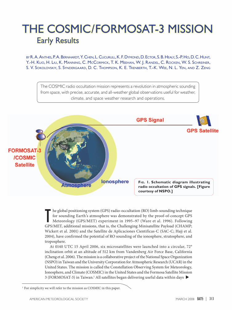
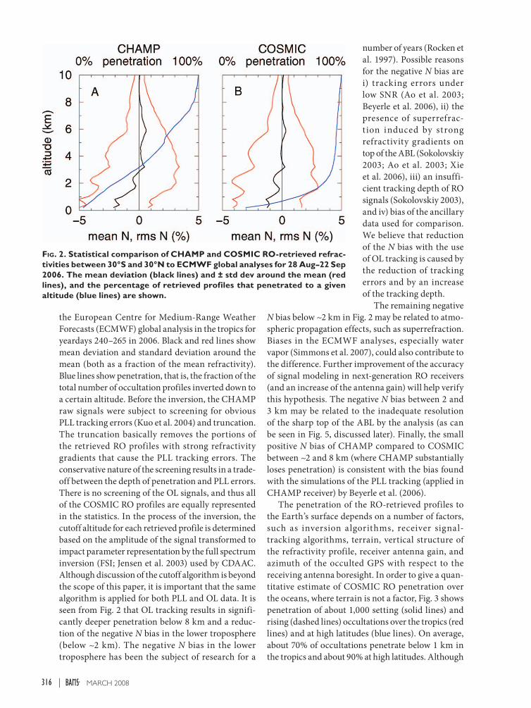
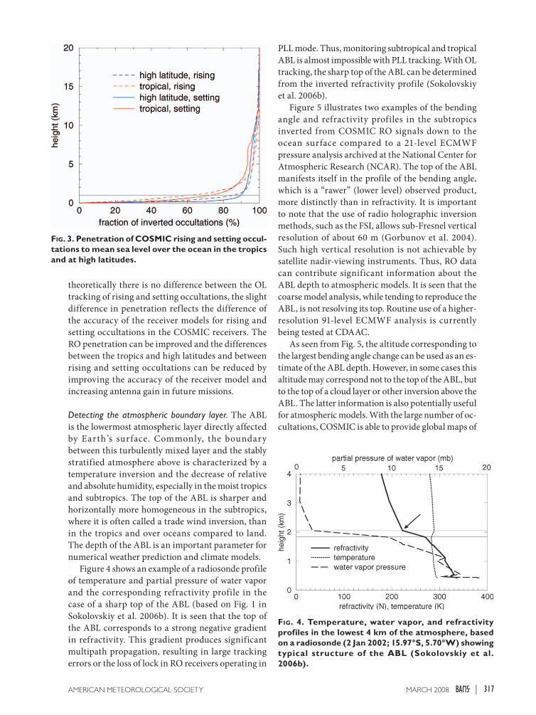
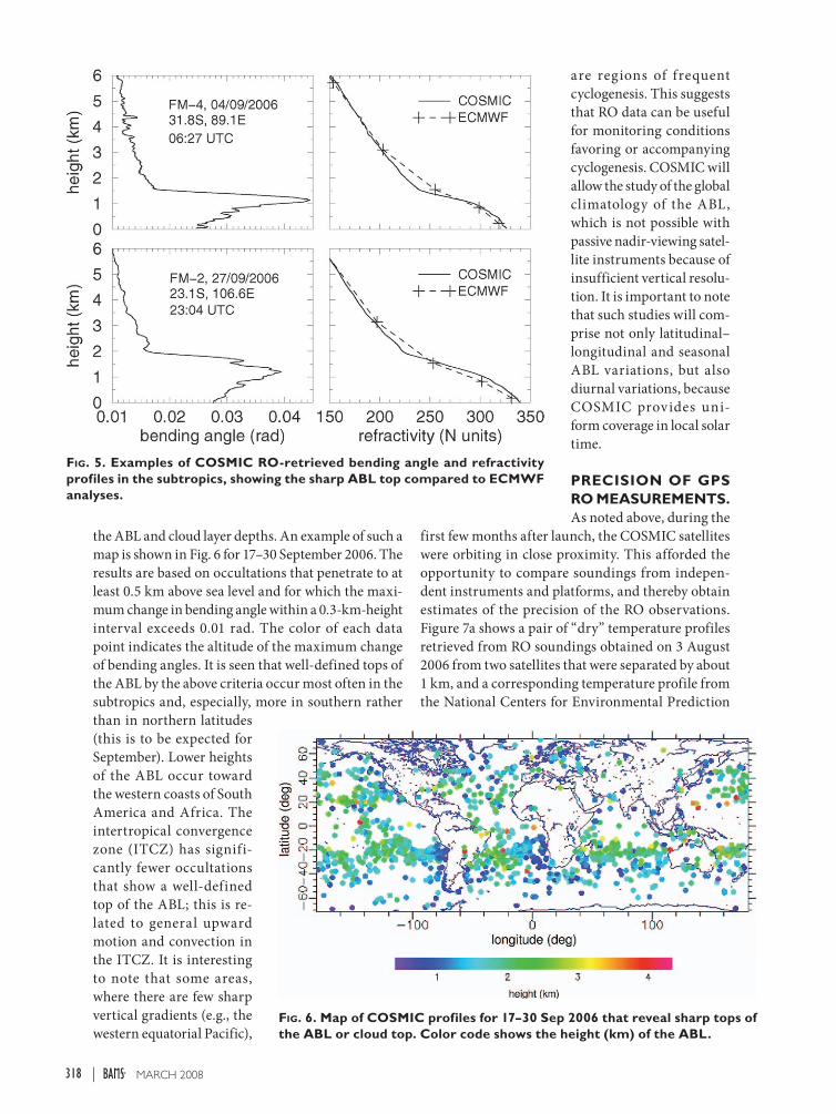
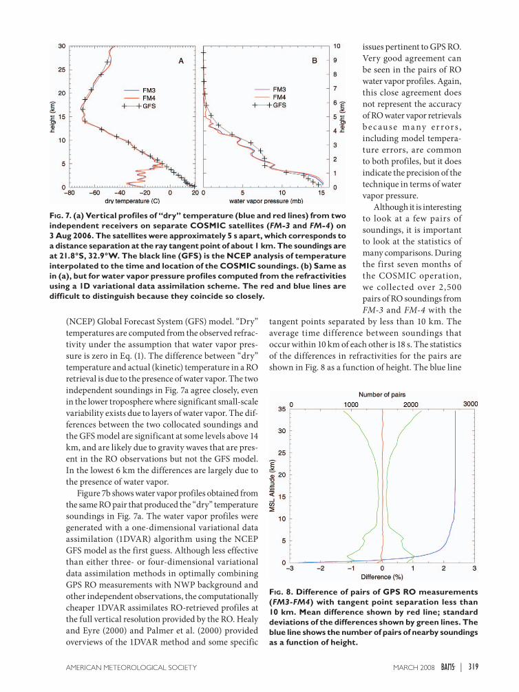
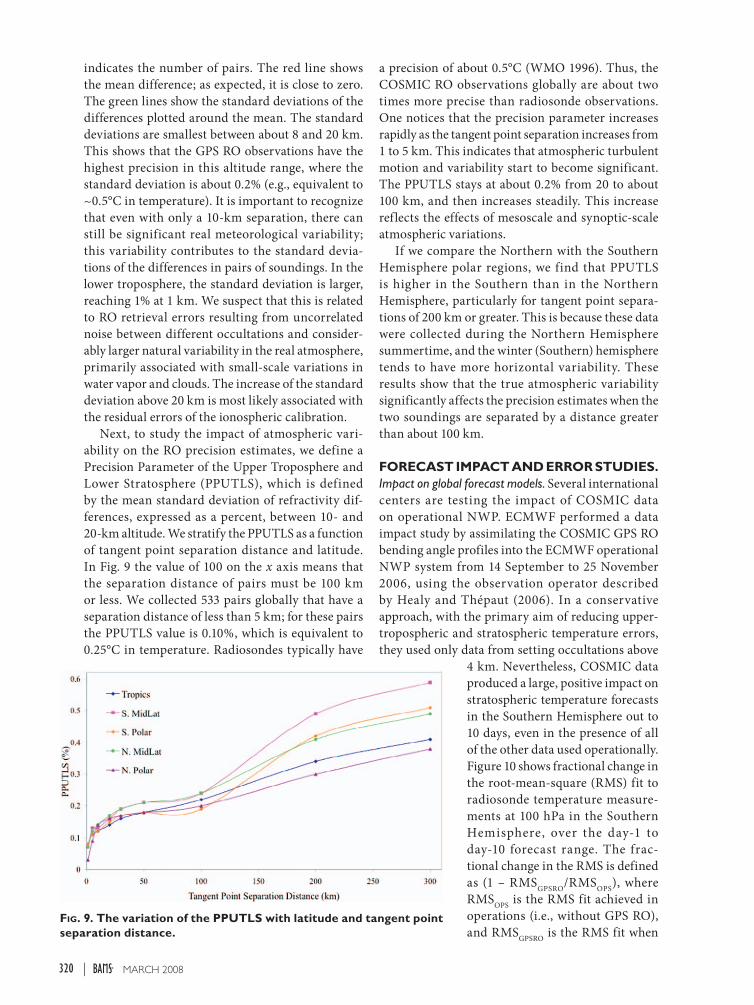
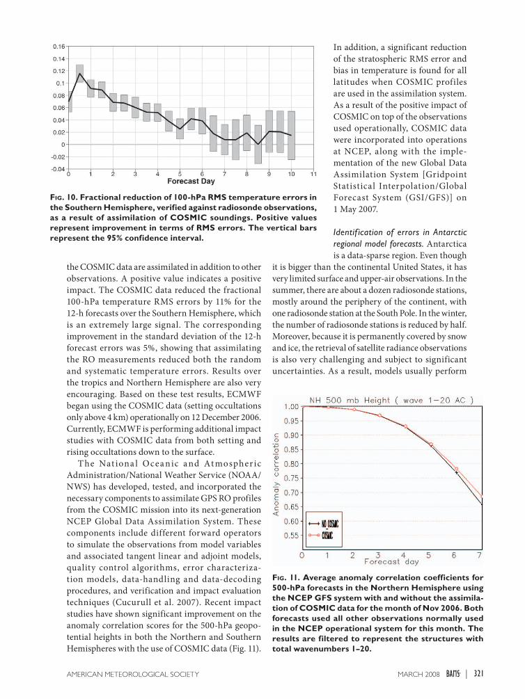
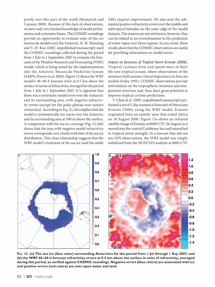
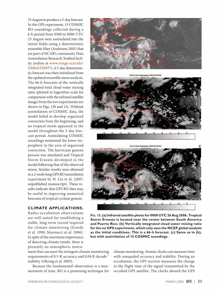
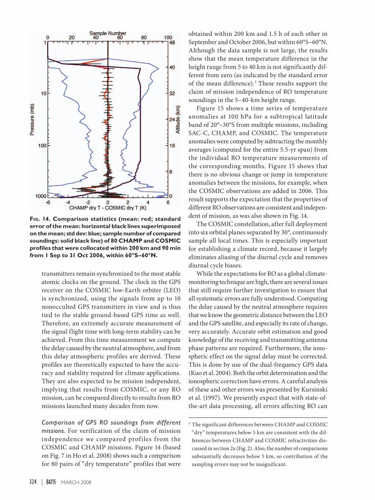
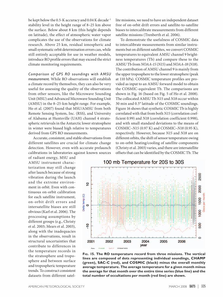
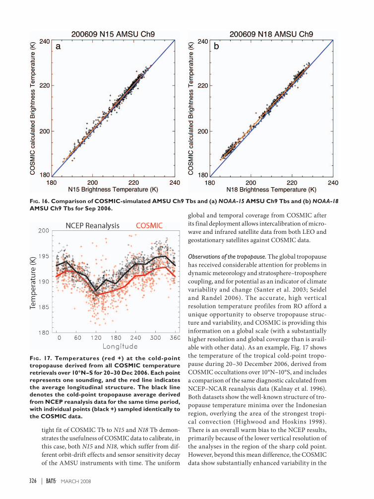
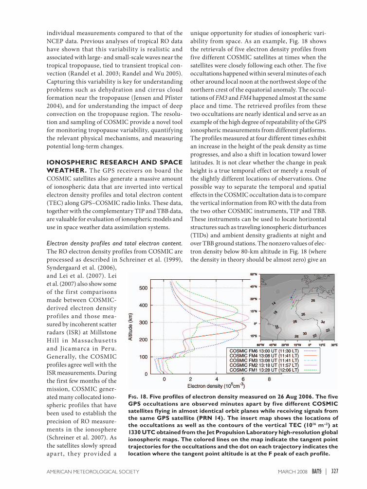
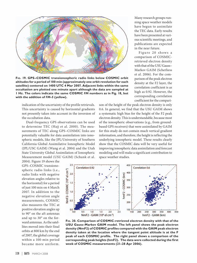
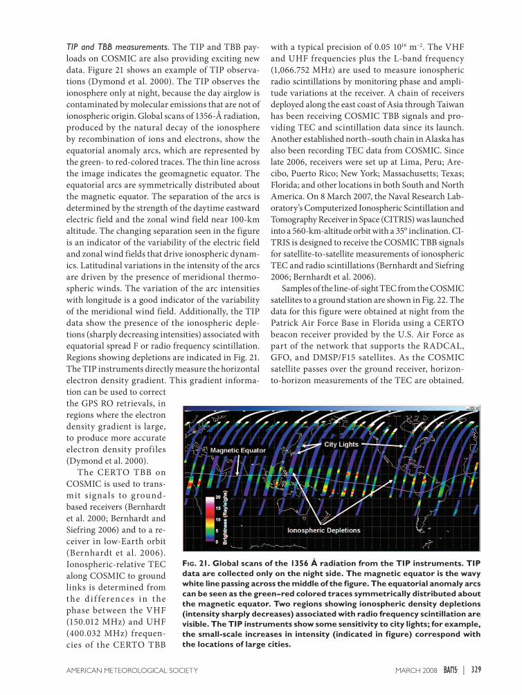
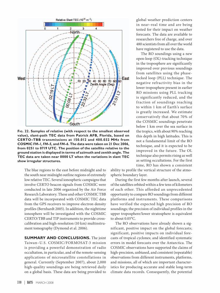
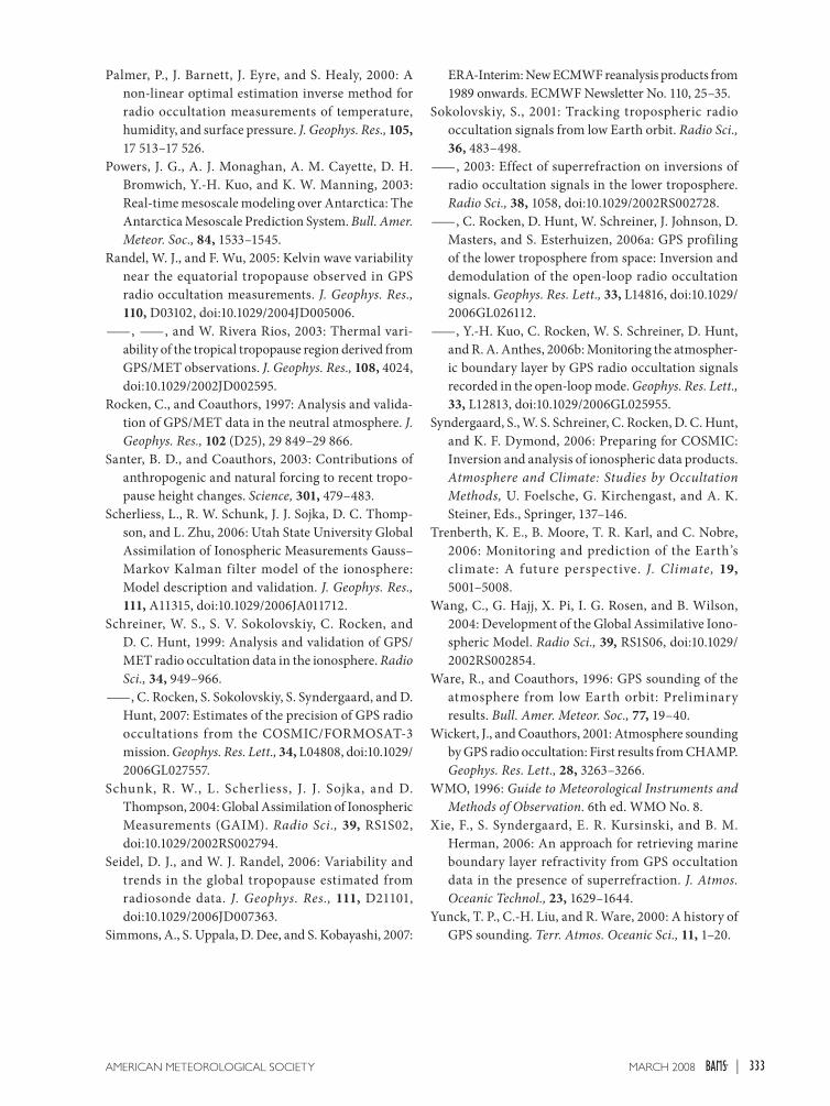
![FORMOSAT-7/COSMIC-2 Neutral Atmosphere Provisional …...FORMOSAT-7/COSMIC-2 Neutral Atmosphere Provisional Data Release 1 References [1] Chen et al., Typhoon Predictions with GNSS](https://static.documents.pub/doc/80x56/5f3c9640d375b5758f36914a/formosat-7cosmic-2-neutral-atmosphere-provisional-formosat-7cosmic-2-neutral.jpg)


