Turbo and LDPC Codes: Implementation, Simulation, and...

1

Turbo and LDPC Codes:Implementation, Simulation,

and Standardization

June 7, 2006

Matthew ValentiRohit Iyer SeshadriWest Virginia UniversityMorgantown, WV [email protected]

6/7/2006Turbo and LDPC Codes

2/133

Tutorial OverviewChannel capacityConvolutional codes – the MAP algorithm

Turbo codes– Standard binary turbo codes: UMTS and cdma2000– Duobinary CRSC turbo codes: DVB-RCS and 802.16

LDPC codes– Tanner graphs and the message passing algorithm– Standard binary LDPC codes: DVB-S2

Bit interleaved coded modulation (BICM)– Combining high-order modulation with a binary capacity

approaching code.EXIT chart analysis of turbo codes

3:15 PMIyer Seshadri

4:30 PMValenti

1:15 PMValenti

2


3/133

Software to Accompany TutorialIterative Solution’s Coded Modulation Library (CML) is a library for simulating and analyzing coded modulation.Available for free at the Iterative Solutions website:– www.iterativesolutions.com

Runs in matlab, but uses c-mex for efficiency.Supported features:– Simulation of BICM

• Turbo, LDPC, or convolutional codes.• PSK, QAM, FSK modulation.• BICM-ID: Iterative demodulation and decoding.

– Generation of ergodic capacity curves (BICM/CM constraints).– Information outage probability in block fading.– Calculation of throughput of hybrid-ARQ.

Implemented standards:– Binary turbo codes: UMTS/3GPP, cdma2000/3GPP2.– Duobinary turbo codes: DVB-RCS, wimax/802.16.– LDPC codes: DVB-S2.


4/133

Noisy Channel Coding TheoremClaude Shannon, “A mathematical theory of communication,” Bell Systems Technical Journal, 1948.Every channel has associated with it a capacity C.– Measured in bits per channel use (modulated symbol).

The channel capacity is an upper bound on information rate r.– There exists a code of rate r < C that achieves reliable communications.

• Reliable means an arbitrarily small error probability.

3


5/133

Computing Channel CapacityThe capacity is the mutual information between the channel’s input X and output Y maximized over all possible input distributions:

C I X Y

p x y p x yp x p y

dxdy

p x

p x

=

=RST

UVWzzmax ( ; )

max , log ( , )( ) ( )

( )

( )

k p

a f 2


6/133

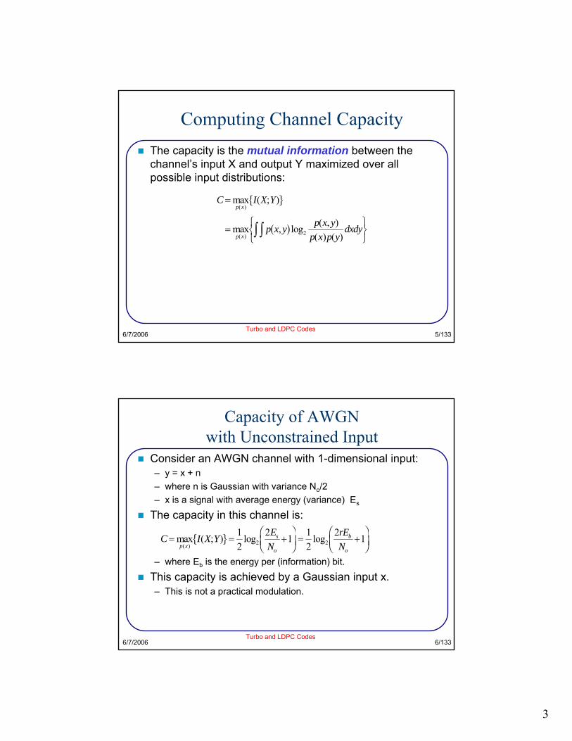
Capacity of AWGNwith Unconstrained Input

Consider an AWGN channel with 1-dimensional input:– y = x + n– where n is Gaussian with variance No/2– x is a signal with average energy (variance) Es

The capacity in this channel is:

– where Eb is the energy per (information) bit.

This capacity is achieved by a Gaussian input x.– This is not a practical modulation.

C I X Y EN

rENp x

s

o

b

o

= = +FHGIKJ = +

FHG

IKJmax ( ; ) log log

( )k p 1

22 1 1

22 12 2

4


7/133

Capacity of AWGN withBPSK Constrained Input

If we only consider antipodal (BPSK) modulation, then

and the capacity is:

X s= ± E

C I X Y

I X Y

H Y H N

p y p y dy eN

p x

p x p

o

=

=

= −

= −

=

−∞

∞z

max ;

;

( ) ( )

log ( ) log

( )

( ): /

a fl qa f

a f b g

1 2

2 212

π

maximized whentwo signals are equally likely

This term must be integrated numerically with

p y p y p y p p y dY X N X N( ) ( ) ( ) ( ) ( )= ∗ = −−∞

∞z λ λ λ

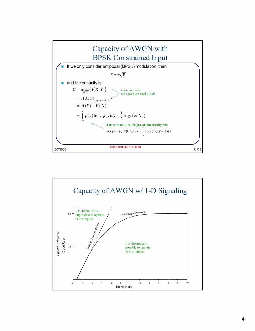
Capacity of AWGN w/ 1-D Signaling

0 1 2 3 4 5 6 7 8 9 10-1-2

0.5

1.0

Eb/No in dB

BPSK Capacity Bound

Cod

e R

ate

r

Shan

non

Capa

city

Boun

d

Spec

tral E

ffici

ency

It is theoreticallypossible to operatein this region.

It is theoreticallyimpossible to operatein this region.

5

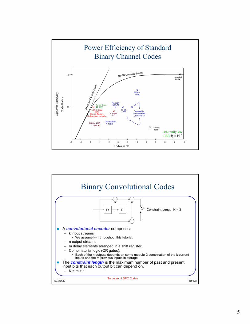
Power Efficiency of StandardBinary Channel Codes

Mariner1969

Turbo Code1993

Galileo:BVD1992Galileo:LGA

1996

Pioneer1968-72

Voyager1977

OdenwalderConvolutionalCodes 1976

0 1 2 3 4 5 6 7 8 9 10-1-2

0.5

1.0

Eb/No in dB

BPSK Capacity Bound

Cod

e R

ate

r

Shan

non

Capa

city

Boun

d

UncodedBPSK

IS-951991

Iridium1998

510−=bP

Spec

tral E

ffici

ency

arbitrarily lowBER:

LDPC Code2001

Chung, Forney,Richardson, Urbanke


10/133

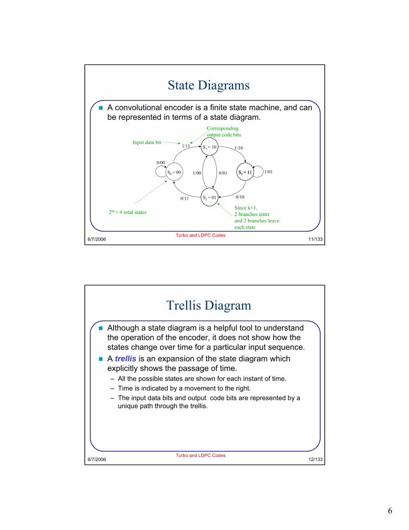
Binary Convolutional Codes

A convolutional encoder comprises:– k input streams

• We assume k=1 throughout this tutorial.– n output streams– m delay elements arranged in a shift register.– Combinatorial logic (OR gates).

• Each of the n outputs depends on some modulo-2 combination of the k current inputs and the m previous inputs in storage

The constraint length is the maximum number of past and present input bits that each output bit can depend on.– K = m + 1

Constraint Length K = 3D D

6


11/133

State DiagramsA convolutional encoder is a finite state machine, and can be represented in terms of a state diagram.

S3 = 11

S2 = 01

S1 = 10

S3 = 11S0 = 00

1/11 1/10

0/11 0/10

1/01

0/00

0/011/00

Input data bit

Corresponding output code bits

2m = 4 total statesSince k=1, 2 branches enter and 2 branches leaveeach state


12/133

Trellis DiagramAlthough a state diagram is a helpful tool to understand the operation of the encoder, it does not show how the states change over time for a particular input sequence.A trellis is an expansion of the state diagram which explicitly shows the passage of time.– All the possible states are shown for each instant of time.– Time is indicated by a movement to the right.– The input data bits and output code bits are represented by a

unique path through the trellis.

7

S0

S3

S2

S1

0/00

1/11

1/10

0/01

1/01

0/10

1/000/11

i = 0 i = 6i = 3i = 2i = 1 i = 4 i = 5

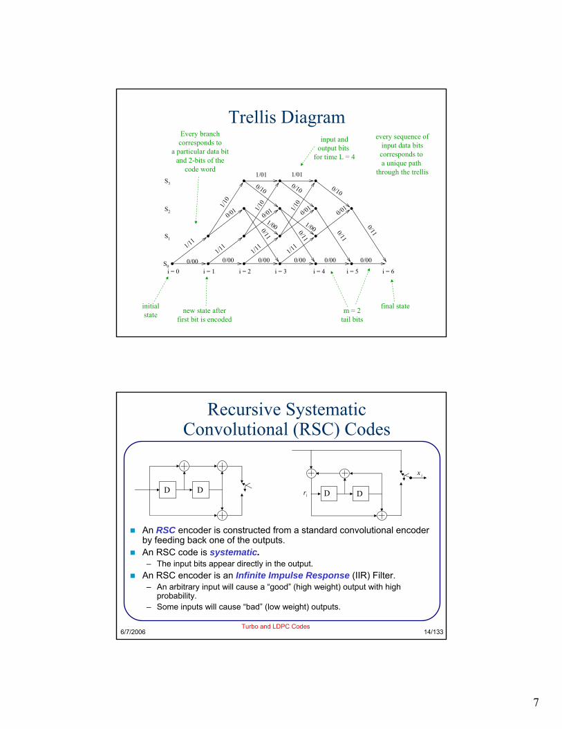
Trellis Diagram

initialstate

Every branchcorresponds to

a particular data bitand 2-bits of the

code word

new state afterfirst bit is encoded

final statem = 2tail bits

1/10

1/10

1/11 1/11 1/11

0/00 0/00 0/00 0/00 0/000/11

0/11

0/11

1/00

0/01 0/010/01

0/10 0/10

every sequence ofinput data bitscorresponds to a unique path

through the trellis1/01

input andoutput bits

for time L = 4


14/133

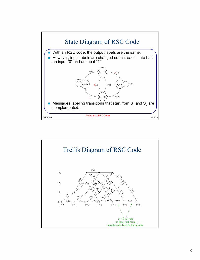
Recursive Systematic Convolutional (RSC) Codes

An RSC encoder is constructed from a standard convolutional encoder by feeding back one of the outputs.An RSC code is systematic.– The input bits appear directly in the output.

An RSC encoder is an Infinite Impulse Response (IIR) Filter. – An arbitrary input will cause a “good” (high weight) output with high

probability.– Some inputs will cause “bad” (low weight) outputs.

D D

ix

irD D

8


15/133

State Diagram of RSC CodeWith an RSC code, the output labels are the same.However, input labels are changed so that each state has an input “0” and an input “1”

Messages labeling transitions that start from S1 and S2 are complemented.

S3 = 11

S2 = 01

S1 = 10

S3 = 11S0 = 00

1/11 0/10

1/11 0/10

1/01

0/00

1/010/00

S0

S3

S2

S1

0/00

1/11

0/10

1/01

1/01

0/10

0/001/11

i = 0 i = 6i = 3i = 2i = 1 i = 4 i = 5

Trellis Diagram of RSC Code

m = 2 tail bitsno longer all-zeros

must be calculated by the encoder

0/10

0/10

1/11 1/11 1/11

0/00 0/00 0/00 0/00 0/00

1/11

1/11

1/11

0/00

1/01 1/011/01

0/10 0/10

9


17/133

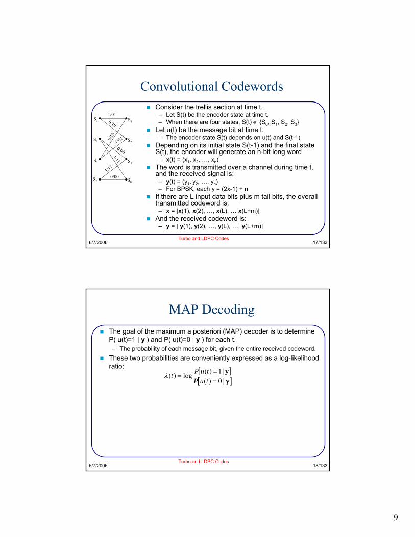
Convolutional CodewordsConsider the trellis section at time t.– Let S(t) be the encoder state at time t.– When there are four states, S(t) ∈ {S0, S1, S2, S3}

Let u(t) be the message bit at time t.– The encoder state S(t) depends on u(t) and S(t-1)

Depending on its initial state S(t-1) and the final state S(t), the encoder will generate an n-bit long word– x(t) = (x1, x2, …, xn)

The word is transmitted over a channel during time t, and the received signal is:– y(t) = (y1, y2, …, yn)– For BPSK, each y = (2x-1) + n

If there are L input data bits plus m tail bits, the overall transmitted codeword is:– x = [x(1), x(2), …, x(L), … x(L+m)]

And the received codeword is:– y = [ y(1), y(2), …, y(L), …, y(L+m)]

0/10

1/11

0/00

1/11

1/01

0/10

S0

S1

S2

S3

S0

S1

S2

S3

1/01

0/00


18/133

MAP DecodingThe goal of the maximum a posteriori (MAP) decoder is to determine P( u(t)=1 | y ) and P( u(t)=0 | y ) for each t.– The probability of each message bit, given the entire received codeword.

These two probabilities are conveniently expressed as a log-likelihood ratio: [ ]

[ ]yy

|0)(|1)(log)(

==

=tuPtuPtλ

10


19/133

Determining Message Bit Probabilitiesfrom the Branch Probabilities

Let pi,j(t) be the probability that the encoder made a transition from Si to Sj at time t, given the entire received codeword.– pi,j(t) = P( Si(t-1) Sj(t) | y )– where Sj(t) means that S(t)=Sj

For each t,

The probability that u(t) = 1 is

Likewise

p 1,3

p 0,1

p0,0

p2,0

p 1,2

p3,2

p3,3

p2,1

S0

S1

S2

S3

S0

S1

S2

S3

1)|)()1(( =→−∑→ ji SS

ji tStSP y

( )∑=→

→−==1:

|)()1()|1)((uSS

jiji

tStSPtuP yy

( )∑=→

→−==0:

|)()1()|0)((uSS

jiji

tStSPtuP yy


20/133

Determining the Branch Probabilities

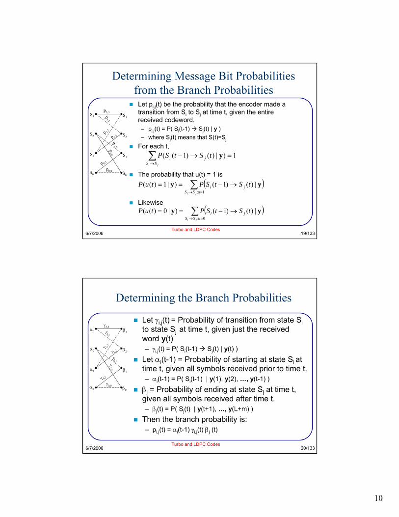
Let γi,j(t) = Probability of transition from state Sito state Sj at time t, given just the received word y(t)– γi,j(t) = P( Si(t-1) Sj(t) | y(t) )

Let αi(t-1) = Probability of starting at state Si at time t, given all symbols received prior to time t.– αi(t-1) = P( Si(t-1) | y(1), y(2), …, y(t-1) )

βj = Probability of ending at state Sj at time t, given all symbols received after time t.– βj(t) = P( Sj(t) | y(t+1), …, y(L+m) )

Then the branch probability is:– pi,j(t) = αi(t-1) γi,j(t) βj (t)

γ 1,3

γ 0,1

γ0,0

γ2,0

γ 1,2

γ3,2

α0

α1

α2

α3

β0

β1

β2

β3

γ3,3

γ2,1

11


21/133

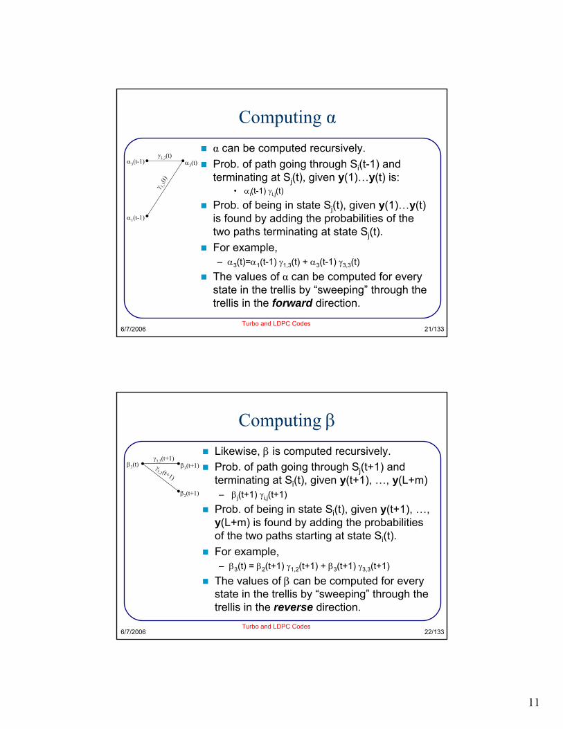
Computing αα can be computed recursively.Prob. of path going through Si(t-1) and terminating at Sj(t), given y(1)…y(t) is:

• αi(t-1) γi,j(t)

Prob. of being in state Sj(t), given y(1)…y(t) is found by adding the probabilities of the two paths terminating at state Sj(t). For example,– α3(t)=α1(t-1) γ1,3(t) + α3(t-1) γ3,3(t)

The values of α can be computed for every state in the trellis by “sweeping” through the trellis in the forward direction.

γ 1,3(t)

α1(t-1)

α3(t-1) α3(t)γ3,3(t)


22/133

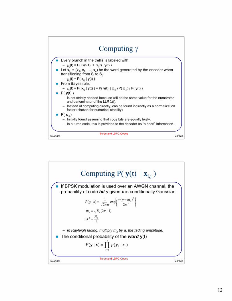
Computing βLikewise, β is computed recursively.Prob. of path going through Sj(t+1) and terminating at Si(t), given y(t+1), …, y(L+m)– βj(t+1) γi,j(t+1)

Prob. of being in state Si(t), given y(t+1), …, y(L+m) is found by adding the probabilities of the two paths starting at state Si(t). For example,– β3(t) = β2(t+1) γ1,2(t+1) + β3(t+1) γ3,3(t+1)

The values of β can be computed for every state in the trellis by “sweeping” through the trellis in the reverse direction.

γ3,2 (t+1)

β3(t)

β2(t+1)

β3(t+1)γ3,3(t+1)

12


23/133

Computing γEvery branch in the trellis is labeled with:– γi,j(t) = P( Si(t-1) Sj(t) | y(t) )

Let xi,j = (x1, x2, …, xn) be the word generated by the encoder when transitioning from Si to Sj.– γi,j(t) = P( xi,j | y(t) )

From Bayes rule,– γi,j(t) = P( xi,j | y(t) ) = P( y(t) | xi,j ) P( xi,j ) / P( y(t) )

P( y(t) )– Is not strictly needed because will be the same value for the numerator

and denominator of the LLR λ(t).– Instead of computing directly, can be found indirectly as a normalization

factor (chosen for numerical stability)P( xi,j )– Initially found assuming that code bits are equally likely.– In a turbo code, this is provided to the decoder as “a priori” information.


24/133

Computing P( y(t) | xi,j ) If BPSK modulation is used over an AWGN channel, the probability of code bit y given x is conditionally Gaussian:

– In Rayleigh fading, multiply mx by a, the fading amplitude.The conditional probability of the word y(t)

2

)12(

2)(exp

21)|(

02

2

2

NxEm

myxyP

sx

x

=

−=⎭⎬⎫

⎩⎨⎧ −−

=

σ

σσπ

∏=

=n

iii xypP

1

)|()|( xy

13


25/133

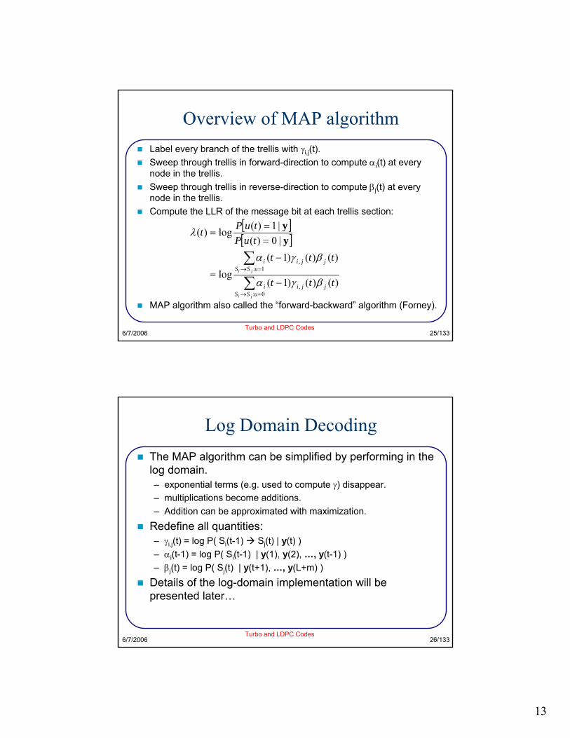
Overview of MAP algorithmLabel every branch of the trellis with γi,j(t).Sweep through trellis in forward-direction to compute αi(t) at every node in the trellis.Sweep through trellis in reverse-direction to compute βj(t) at every node in the trellis.Compute the LLR of the message bit at each trellis section:

MAP algorithm also called the “forward-backward” algorithm (Forney).

[ ][ ]

∑

∑

=→

=→

−

−

=

==

=

0:,

1:,

)()()1(

)()()1(log

|0)(|1)(log)(

uSSjjii

uSSjjii

ji

ji

ttt

ttttuPtuPt

βγα

βγα

λyy


26/133

Log Domain DecodingThe MAP algorithm can be simplified by performing in the log domain.– exponential terms (e.g. used to compute γ) disappear.– multiplications become additions.– Addition can be approximated with maximization.

Redefine all quantities:– γi,j(t) = log P( Si(t-1) Sj(t) | y(t) )– αi(t-1) = log P( Si(t-1) | y(1), y(2), …, y(t-1) )– βj(t) = log P( Sj(t) | y(t+1), …, y(L+m) )

Details of the log-domain implementation will be presented later…

14


27/133

Parallel Concatenated Codeswith Nonuniform Interleaving

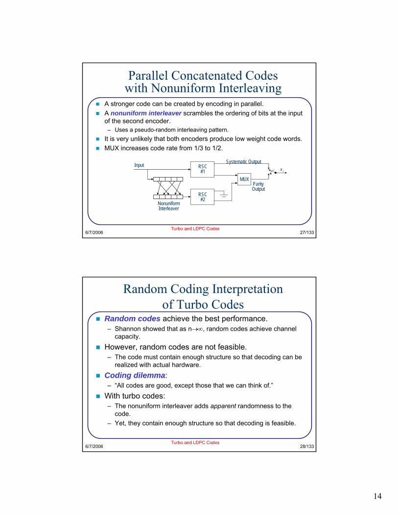
A stronger code can be created by encoding in parallel.A nonuniform interleaver scrambles the ordering of bits at the input of the second encoder.– Uses a pseudo-random interleaving pattern.

It is very unlikely that both encoders produce low weight code words.MUX increases code rate from 1/3 to 1/2.

RSC#1

RSC#2

NonuniformInterleaver

MUX

Input

ParityOutput

Systematic Outputix


28/133

Random Coding Interpretationof Turbo Codes

Random codes achieve the best performance.– Shannon showed that as n→∞, random codes achieve channel

capacity.

However, random codes are not feasible.– The code must contain enough structure so that decoding can be

realized with actual hardware.

Coding dilemma:– “All codes are good, except those that we can think of.”

With turbo codes:– The nonuniform interleaver adds apparent randomness to the

code.– Yet, they contain enough structure so that decoding is feasible.

15


29/133

Comparison of a Turbo Codeand a Convolutional Code

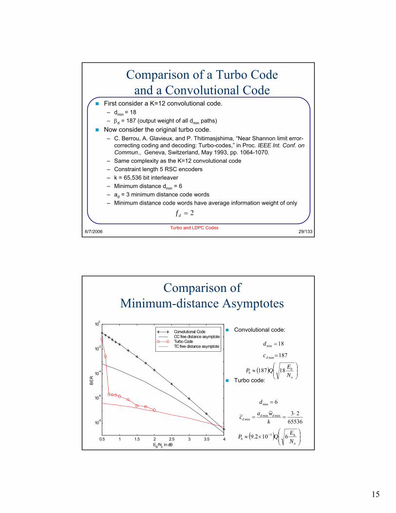
First consider a K=12 convolutional code.– dmin = 18– βd = 187 (output weight of all dmin paths)

Now consider the original turbo code.– C. Berrou, A. Glavieux, and P. Thitimasjshima, “Near Shannon limit error-

correcting coding and decoding: Turbo-codes,” in Proc. IEEE Int. Conf. on Commun., Geneva, Switzerland, May 1993, pp. 1064-1070.

– Same complexity as the K=12 convolutional code– Constraint length 5 RSC encoders– k = 65,536 bit interleaver– Minimum distance dmin = 6– ad = 3 minimum distance code words– Minimum distance code words have average information weight of only

f d = 2

0.5 1 1.5 2 2.5 3 3.5 4

10-8

10-6

10-4

10-2

100

Eb/No in dB

BE

R

Convolutional Code CC free distance asymptoteTurbo Code TC free distance asymptote

Comparison of Minimum-distance Asymptotes

Convolutional code:

Turbo code:

( ) ⎟⎟⎠

⎞⎜⎜⎝

⎛≈

o

bb N

EQP 18187

( ) ⎟⎟⎠

⎞⎜⎜⎝

⎛×≈ −

o

bb N

EQP 6102.9 5

187min =dc

18min =d

6min =d

6553623~~ minmin

min⋅

==kwac dd

d

16


31/133

The Turbo-PrincipleTurbo codes get their name because the decoder uses feedback, like a turbo engine.

0.5 1 1.5 210-7

10-6

10-5

10-4

10-3

10-2

10-1

100

Eb/No in dB

BE

R

1 iteration

2 iterations

3 iterations6 iterations

10 iterations

18 iterations

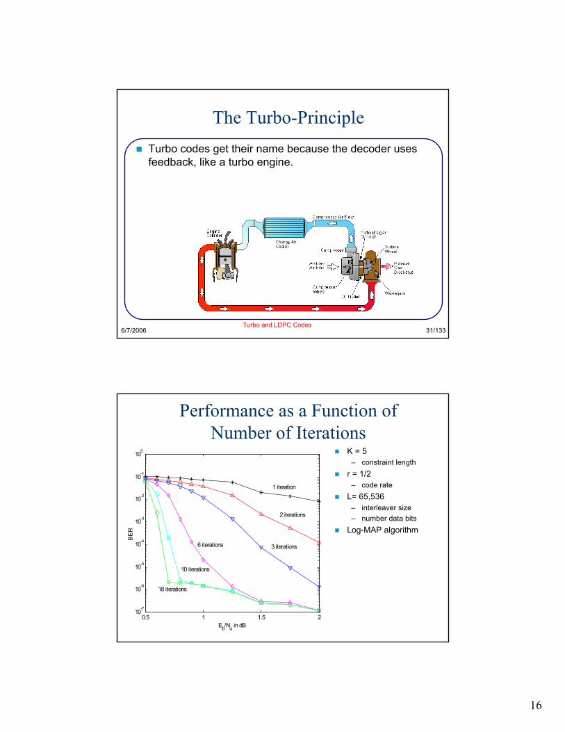
Performance as a Function of Number of Iterations

K = 5– constraint length

r = 1/2– code rate

L= 65,536 – interleaver size– number data bits

Log-MAP algorithm

17


33/133

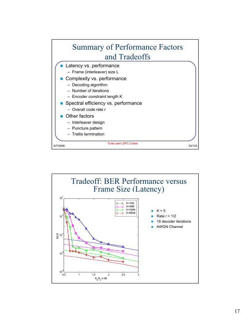
Summary of Performance Factors and Tradeoffs

Latency vs. performance– Frame (interleaver) size L

Complexity vs. performance– Decoding algorithm– Number of iterations– Encoder constraint length K

Spectral efficiency vs. performance– Overall code rate r

Other factors– Interleaver design– Puncture pattern– Trellis termination

0.5 1 1.5 2 2.510

-7

10-6

10-5

10-4

10-3

10-2

10-1

Tradeoff: BER Performance versus Frame Size (Latency)

K = 5Rate r = 1/218 decoder iterationsAWGN Channel

0.5 1 1.5 2 2.5 310

-8

10-6

10-4

10-2

100

Eb/No in dB

BE

R

K=1024 K=4096 K=16384K=65536

18


35/133

Characteristics of Turbo CodesTurbo codes have extraordinary performance at low SNR.– Very close to the Shannon limit.– Due to a low multiplicity of low weight code words.

However, turbo codes have a BER “floor”.– This is due to their low minimum distance.

Performance improves for larger block sizes.– Larger block sizes mean more latency (delay).– However, larger block sizes are not more complex to decode.– The BER floor is lower for larger frame/interleaver sizes

The complexity of a constraint length KTC turbo code is the same as a K = KCC convolutional code, where:– KCC ≈ 2+KTC+ log2(number decoder iterations)

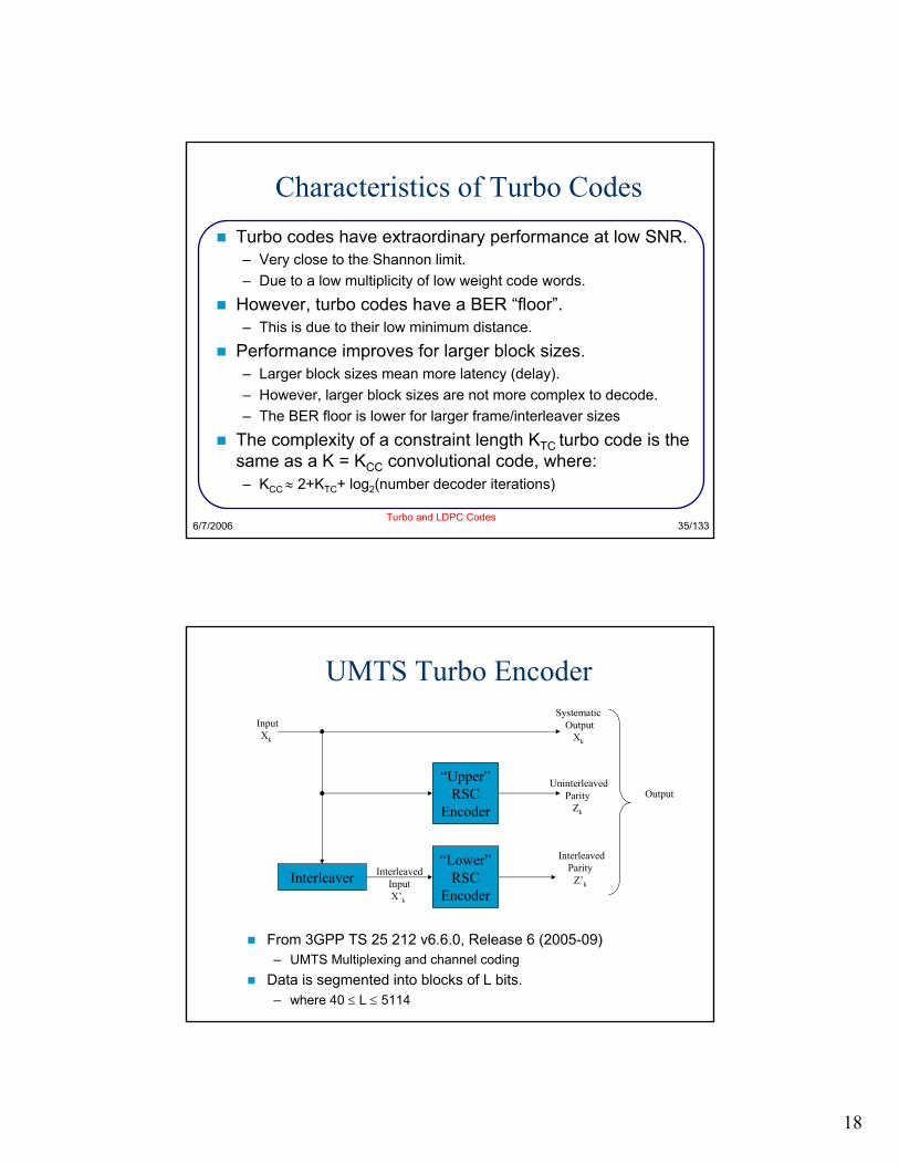
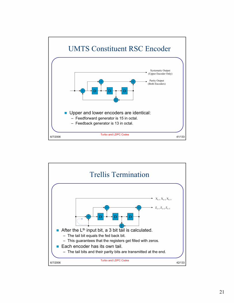
UMTS Turbo Encoder

From 3GPP TS 25 212 v6.6.0, Release 6 (2005-09)– UMTS Multiplexing and channel coding

Data is segmented into blocks of L bits. – where 40 ≤ L ≤ 5114

“Upper”RSC

Encoder

“Lower”RSC

EncoderInterleaver

Systematic Output

Xk

UninterleavedParity

Zk

InterleavedParity

Z’k

InputXk

InterleavedInputX’k

Output

19


37/133

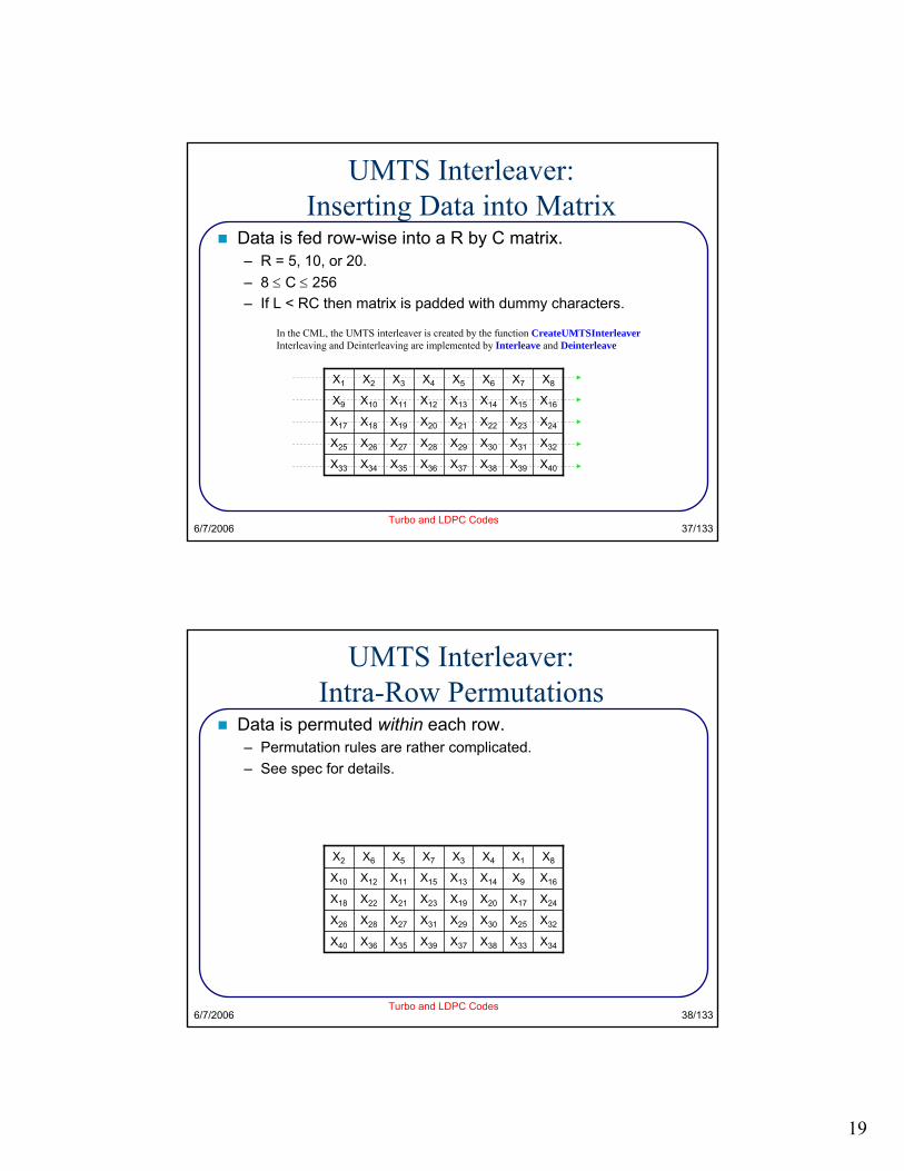
UMTS Interleaver:Inserting Data into Matrix

Data is fed row-wise into a R by C matrix.– R = 5, 10, or 20.– 8 ≤ C ≤ 256– If L < RC then matrix is padded with dummy characters.

X40X39X38X37X36X35X34X33

X32X31X30X29X28X27X26X25

X24X23X22X21X20X19X18X17

X16X15X14X13X12X11X10X9

X8X7X6X5X4X3X2X1

In the CML, the UMTS interleaver is created by the function CreateUMTSInterleaverInterleaving and Deinterleaving are implemented by Interleave and Deinterleave


38/133

UMTS Interleaver:Intra-Row Permutations

Data is permuted within each row.– Permutation rules are rather complicated.– See spec for details.

X34X33X38X37X39X35X36X40

X32X25X30X29X31X27X28X26

X24X17X20X19X23X21X22X18

X16X9X14X13X15X11X12X10

X8X1X4X3X7X5X6X2

20


39/133

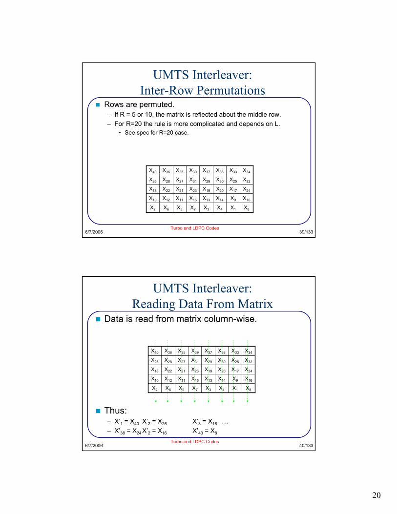
UMTS Interleaver:Inter-Row Permutations

Rows are permuted.– If R = 5 or 10, the matrix is reflected about the middle row.– For R=20 the rule is more complicated and depends on L.

• See spec for R=20 case.

X8X1X4X3X7X5X6X2

X16X9X14X13X15X11X12X10

X24X17X20X19X23X21X22X18

X32X25X30X29X31X27X28X26

X34X33X38X37X39X35X36X40


40/133

UMTS Interleaver:Reading Data From Matrix

Data is read from matrix column-wise.

Thus:– X’1 = X40 X’2 = X26 X’3 = X18 …– X’38 = X24 X’2 = X16 X’40 = X8

X8X1X4X3X7X5X6X2

X16X9X14X13X15X11X12X10

X24X17X20X19X23X21X22X18

X32X25X30X29X31X27X28X26

X34X33X38X37X39X35X36X40

21


41/133

UMTS Constituent RSC Encoder

Upper and lower encoders are identical:– Feedforward generator is 15 in octal.– Feedback generator is 13 in octal.

D D D

Parity Output(Both Encoders)

Systematic Output(Upper Encoder Only)


42/133

Trellis Termination

After the Lth input bit, a 3 bit tail is calculated.– The tail bit equals the fed back bit.– This guarantees that the registers get filled with zeros.

Each encoder has its own tail.– The tail bits and their parity bits are transmitted at the end.

D D D

XL+1 XL+2 XL+3

ZL+1 ZL+2 ZL+3

22


43/133

Output Stream FormatThe format of the output steam is:

X1 Z1 Z’1 X2 Z2 Z’2 … XL ZL Z’L XL+1 ZL+1 XL+2 ZL+2 XL+3 ZL+3 X’L+1 Z’L+1 X’L+2 Z’L+2 X’L+3 Z’L+3

L data bits andtheir associated2L parity bits

(total of 3L bits)

3 tail bits forupper encoder

and their3 parity bits

3 tail bits forlower encoder

and their3 parity bits

Total number of coded bits = 3L + 12

Code rate: r LL

=+

≈3 12

13


44/133

Channel Modeland LLRs

Channel gain: a– Rayleigh random variable if Rayleigh fading– a = 1 if AWGN channel

Noise– variance is:

BPSKModulator

{0,1} {-1,1}

a n2

2σ

a

ry

⎟⎟⎠

⎞⎜⎜⎝

⎛≈

⎟⎟⎠

⎞⎜⎜⎝

⎛=

o

b

o

b

NE

NEr 2

3

2

12σ

23


45/133

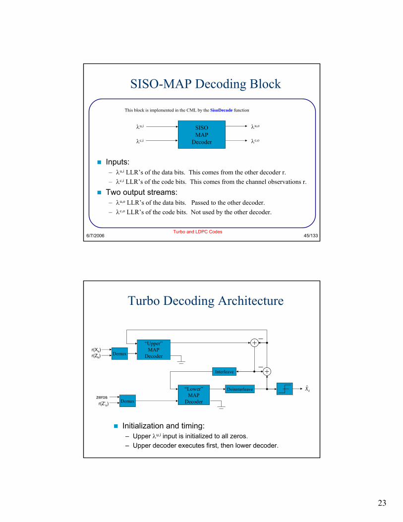
SISO-MAP Decoding Block

Inputs:– λu,i LLR’s of the data bits. This comes from the other decoder r.– λc,i LLR’s of the code bits. This comes from the channel observations r.

Two output streams:– λu,o LLR’s of the data bits. Passed to the other decoder.– λc,o LLR’s of the code bits. Not used by the other decoder.

SISOMAP

Decoder

This block is implemented in the CML by the SisoDecode function

λu,i

λc,i

λu,o

λc,o

Turbo Decoding Architecture

“Upper”MAP

Decoderr(Xk)r(Zk)

“Lower”MAP

Decoderr(Z’k)

Initialization and timing:– Upper λu,i input is initialized to all zeros.– Upper decoder executes first, then lower decoder.

$Xk

Interleave

Deinnterleave

Demux

zerosDemux

24

0 0.2 0.4 0.6 0.8 1 1.2 1.4 1.6 1.8 210

-7

10-6

10-5

10-4

10-3

10-2

10-1

100

Eb/No in dB

BE

R

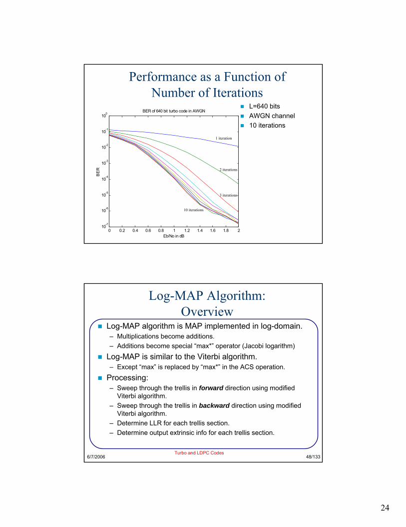
BER of 640 bit turbo code in AWGN

Performance as a Function of Number of Iterations

L=640 bitsAWGN channel10 iterations

1 iteration

2 iterations

3 iterations

10 iterations


48/133

Log-MAP Algorithm:Overview

Log-MAP algorithm is MAP implemented in log-domain.– Multiplications become additions.– Additions become special “max*” operator (Jacobi logarithm)

Log-MAP is similar to the Viterbi algorithm.– Except “max” is replaced by “max*” in the ACS operation.

Processing:– Sweep through the trellis in forward direction using modified

Viterbi algorithm.– Sweep through the trellis in backward direction using modified

Viterbi algorithm.– Determine LLR for each trellis section.– Determine output extrinsic info for each trellis section.

25


49/133

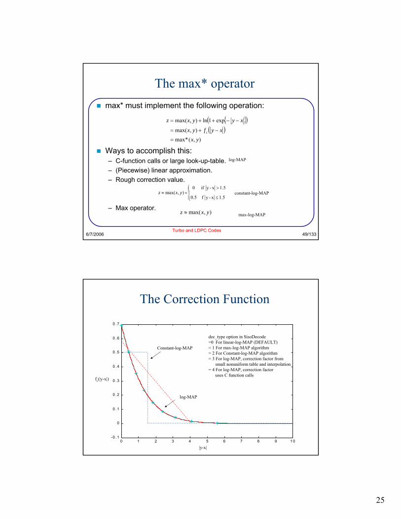
The max* operatormax* must implement the following operation:

Ways to accomplish this:– C-function calls or large look-up-table.– (Piecewise) linear approximation.– Rough correction value.

– Max operator.

{ }( )( )

),(max*),max(

exp1ln),max(

yxxyfyx

xyyxz

c

=

−+=

−−++=

),max( yxz ≈

⎪⎩

⎪⎨⎧

≤

>+≈

5.1x-y f5.0

5.1x-y if0),max( yxz

log-MAP

constant-log-MAP

max-log-MAP

0 1 2 3 4 5 6 7 8 9 1 0-0 .1

0

0 .1

0 .2

0 .3

0 .4

0 .5

0 .6

0 .7

The Correction Function

Constant-log-MAP

log-MAP

|y-x|

fc(|y-x|)

dec_type option in SisoDecode=0 For linear-log-MAP (DEFAULT)= 1 For max-log-MAP algorithm = 2 For Constant-log-MAP algorithm= 3 For log-MAP, correction factor from

small nonuniform table and interpolation= 4 For log-MAP, correction factor

uses C function calls

26


51/133

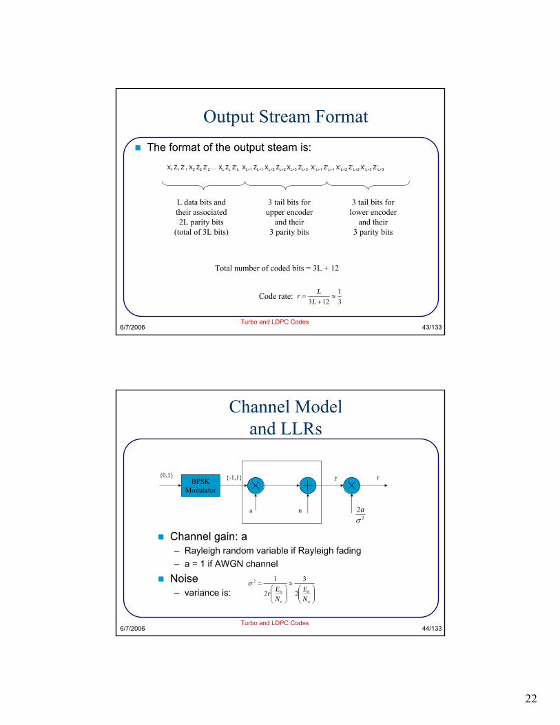
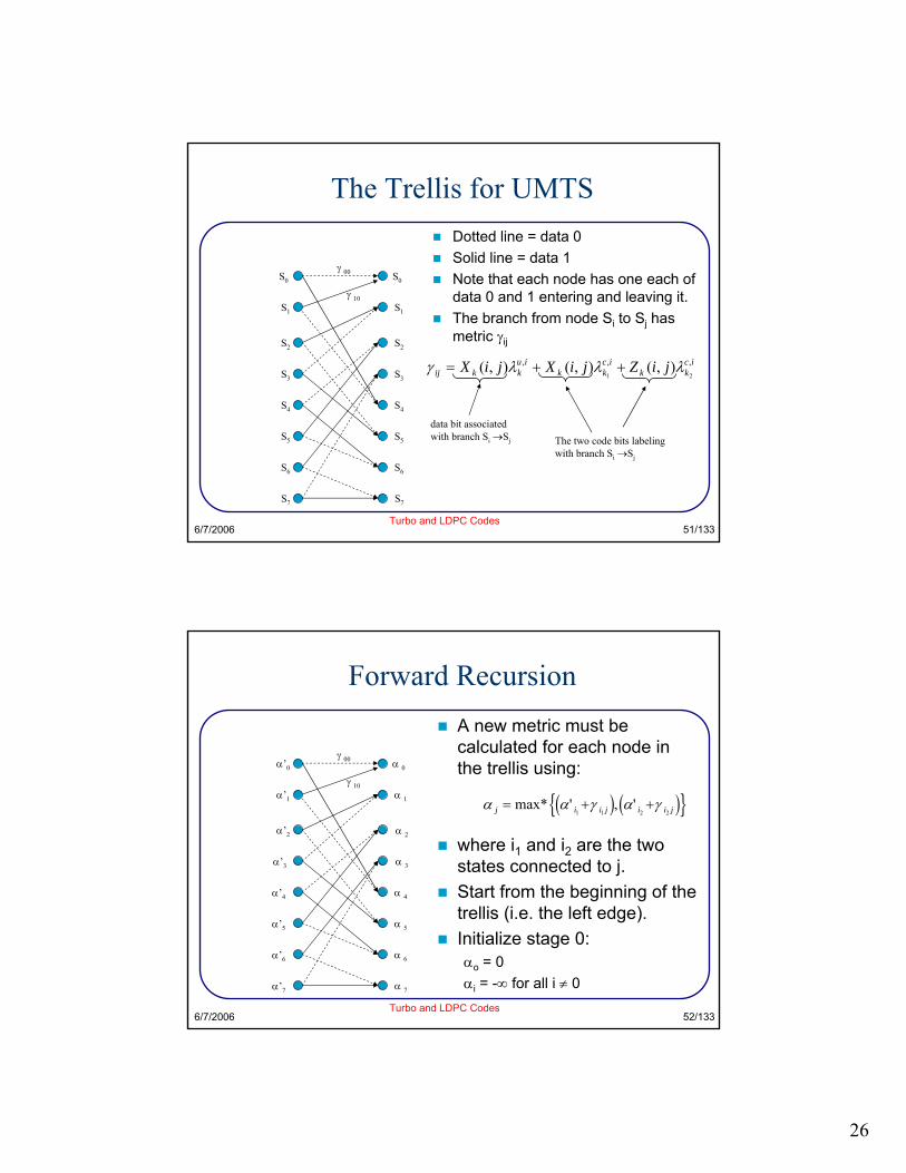
The Trellis for UMTSDotted line = data 0Solid line = data 1Note that each node has one each of data 0 and 1 entering and leaving it.The branch from node Si to Sj has metric γij

S0

S1

S2

S3

S4

S5

S6

S7

S0

S1

S2

S3

S4

S5

S6

S7

γ 00

γ 10

ickk

ickk

iukkij jiZjiXjiX ,,,

21),(),(),( λλλγ ++=

data bit associatedwith branch Si →Sj The two code bits labeling

with branch Si →Sj


52/133

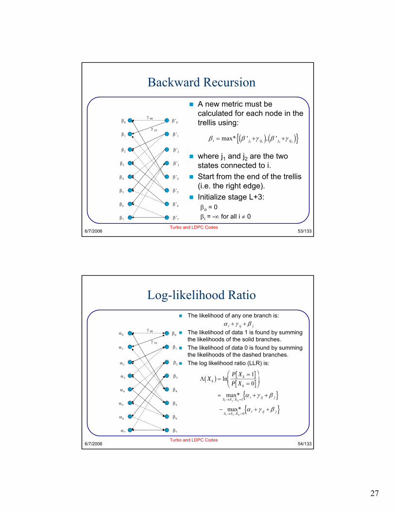
Forward RecursionA new metric must be calculated for each node in the trellis using:

where i1 and i2 are the two states connected to j.Start from the beginning of the trellis (i.e. the left edge).Initialize stage 0:αo = 0αi = -∞ for all i ≠ 0

α’0

α’1

α’2

α 0

α 1

α 2

α 3

α 4

α 5

α 6

α 7

γ 00

γ 10

α’3

α’4

α’5

α’6

α’7

α α γ α γj i i j i i j= + +max* ' , '1 1 2 2d i d io t

27


53/133

Backward RecursionA new metric must be calculated for each node in the trellis using:

where j1 and j2 are the two states connected to i.Start from the end of the trellis (i.e. the right edge).Initialize stage L+3:βo = 0βi = -∞ for all i ≠ 0

β0

β1

β2

β’0

β’1

β’2

β’3

β’4

β’5

β’6

β’7

γ 00

γ 10

β3

β4

β5

β6

β7

β β γ β γi j ij j ij= + +max* ' , ' 1 1 2 2d i d io t


54/133

Log-likelihood RatioThe likelihood of any one branch is:

The likelihood of data 1 is found by summing the likelihoods of the solid branches.The likelihood of data 0 is found by summing the likelihoods of the dashed branches.The log likelihood ratio (LLR) is:

α0

α1

α2

β0

β1

β2

β3

β4

β5

β6

β7

γ 00

γ 10

α3

α4

α5

α6

α7

α γ βi ij j+ +

Λ XP XP Xk

k

k

S S X i ij j

S S X i ij j

i j k

i j k

b g

n sn s

===

FHG

IKJ

= + +

− + +

→ =

→ =

ln

max*

max*

:

:

10

1

0

α γ β

α γ β

28


55/133

Memory IssuesA naïve solution:– Calculate α’s for entire trellis (forward sweep), and store.– Calculate β’s for the entire trellis (backward sweep), and store.– At the kth stage of the trellis, compute λ by combining γ’s with stored α’s

and β’s .A better approach:– Calculate β’s for the entire trellis and store.– Calculate α’s for the kth stage of the trellis, and immediately compute λ by

combining γ’s with these α’s and stored β’s .– Use the α’s for the kth stage to compute α’s for state k+1.

Normalization:– In log-domain, α’s can be normalized by subtracting a common term from

all α’s at the same stage.– Can normalize relative to α0, which eliminates the need to store α0– Same for the β’s


56/133

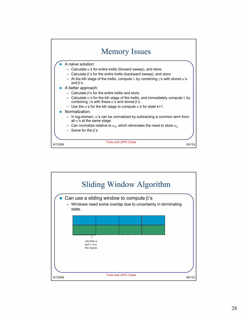
Sliding Window AlgorithmCan use a sliding window to compute β’s– Windows need some overlap due to uncertainty in terminating

state.

assume these statesare equally likely

use thesevalues for β

calculate αand λ overthis region.

initialization region

29


57/133

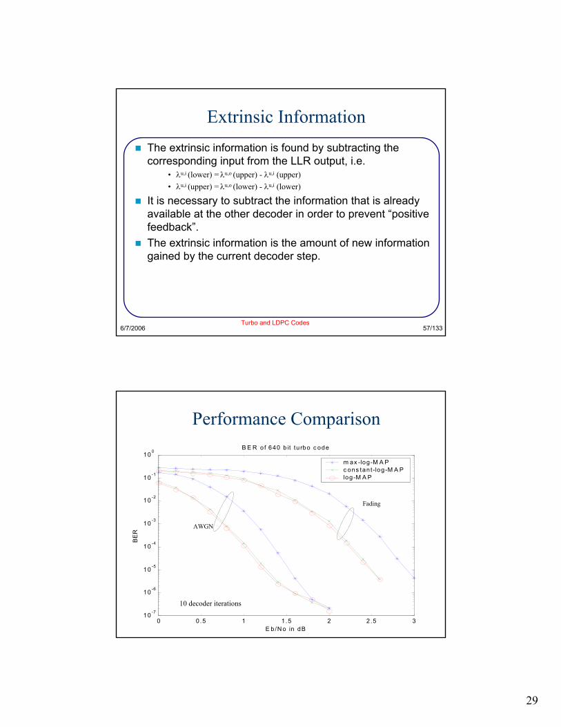
Extrinsic InformationThe extrinsic information is found by subtracting the corresponding input from the LLR output, i.e.

• λu,i (lower) = λu,o (upper) - λu,i (upper)• λu,i (upper) = λu,o (lower) - λu,i (lower)

It is necessary to subtract the information that is already available at the other decoder in order to prevent “positive feedback”.The extrinsic information is the amount of new information gained by the current decoder step.

Performance Comparison

0 0.5 1 1.5 2 2.5 310 -7

10 -6

10 -5

10 -4

10 -3

10 -2

10 -1

10 0

E b/N o in dB

BE

R

B E R o f 640 b it tu rbo c ode

m ax -log-M A P c ons tant-log-M A Plog-M A P

10 decoder iterations

Fading

AWGN

30


59/133

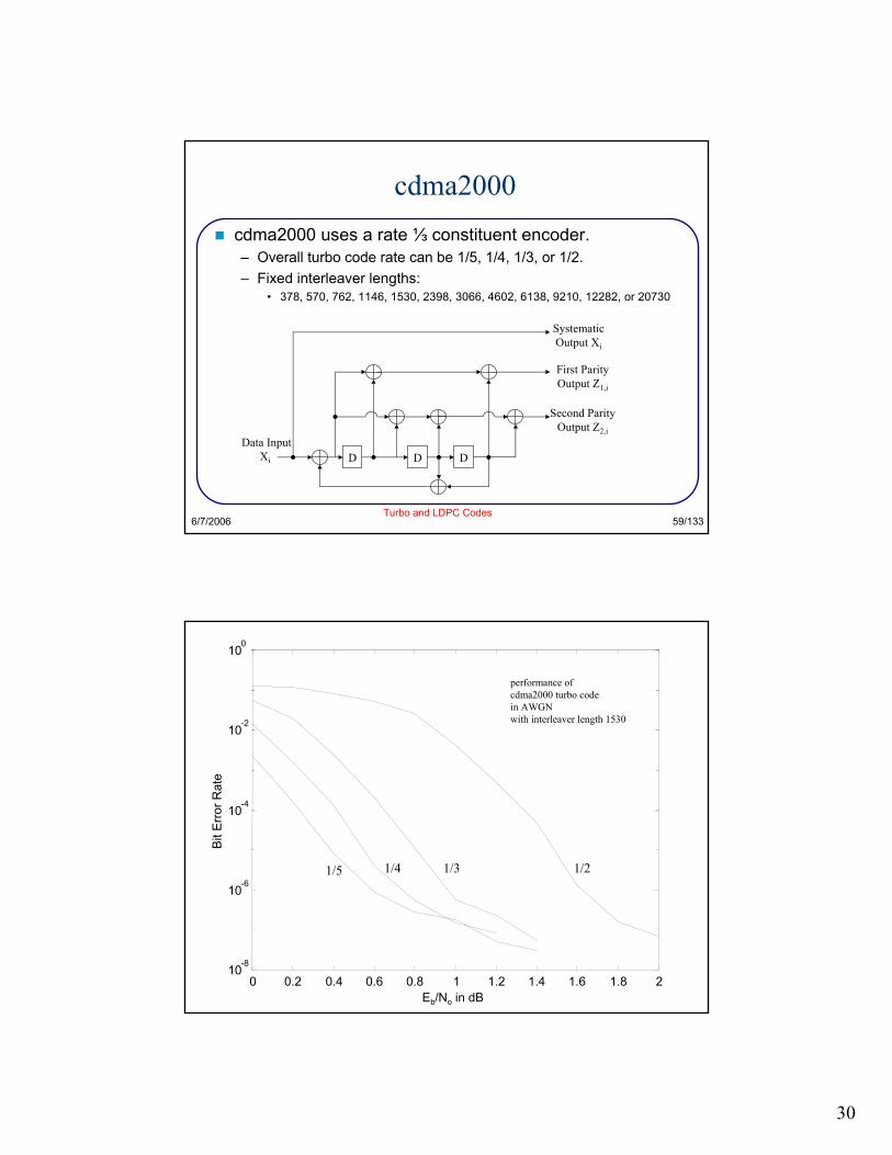
cdma2000cdma2000 uses a rate ⅓ constituent encoder.– Overall turbo code rate can be 1/5, 1/4, 1/3, or 1/2.– Fixed interleaver lengths:

• 378, 570, 762, 1146, 1530, 2398, 3066, 4602, 6138, 9210, 12282, or 20730

D D D

First Parity Output Z1,i

Systematic Output Xi

Data InputXi

Second Parity Output Z2,i

0 0.2 0.4 0.6 0.8 1 1.2 1.4 1.6 1.8 210-8

10-6

10-4

10-2

100

Eb/No in dB

Bit

Erro

r Rat

e

1/21/31/41/5

performance ofcdma2000 turbo codein AWGNwith interleaver length 1530

31


61/133

Circular Recursive Systematic Convolutional (CRSC) Codes

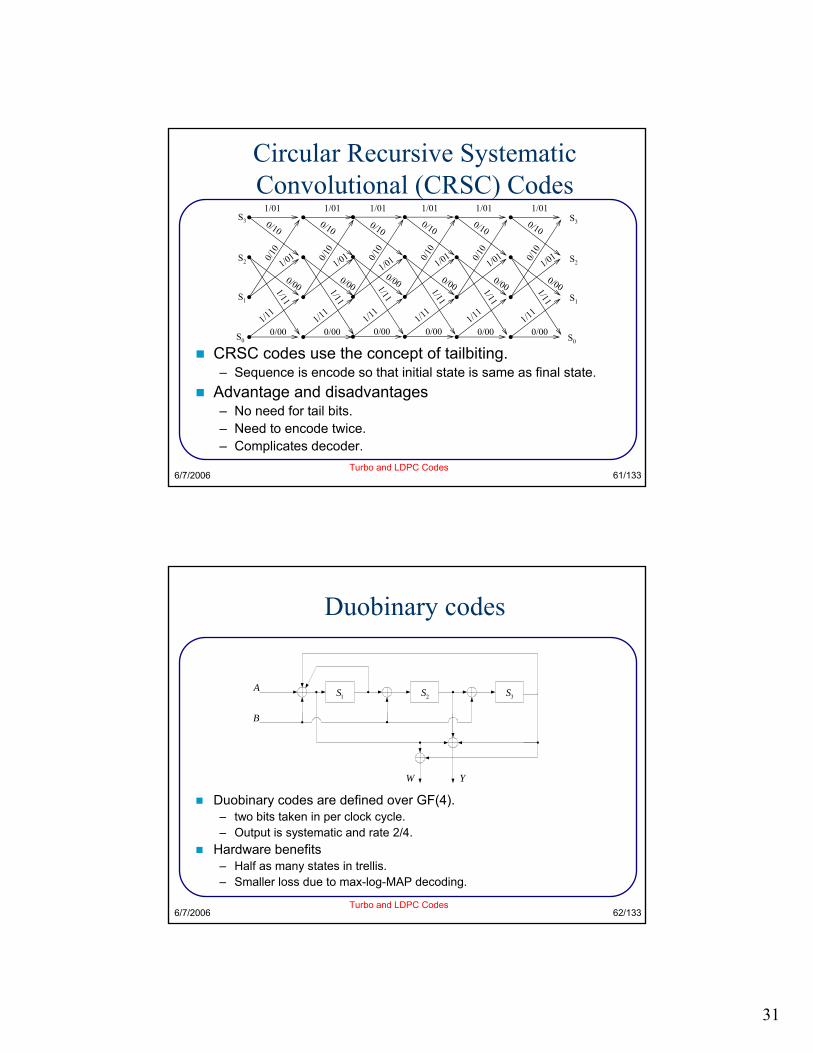
CRSC codes use the concept of tailbiting.– Sequence is encode so that initial state is same as final state.

Advantage and disadvantages – No need for tail bits.– Need to encode twice.– Complicates decoder.

S0

S3

S2

S1

1/01

0/10

0/001/11

0/10

0/10

1/11 1/11

0/00 0/00

1/11

0/00

1/01 1/01

0/10

0/10

1/11

0/001/11

0/00

1/01

0/10

0/10

1/11

0/00

1/110/00

1/01

0/10

0/10

1/11

0/00

1/11

0/00

1/01

0/10

0/10

1/11

0/00

1/11

0/00

1/01

0/10

S0

S3

S2

S1

1/01 1/01 1/011/011/01


62/133

Duobinary codes

Duobinary codes are defined over GF(4).– two bits taken in per clock cycle.– Output is systematic and rate 2/4.

Hardware benefits– Half as many states in trellis.– Smaller loss due to max-log-MAP decoding.

1S 2S 3S

W Y

A

B

32


63/133

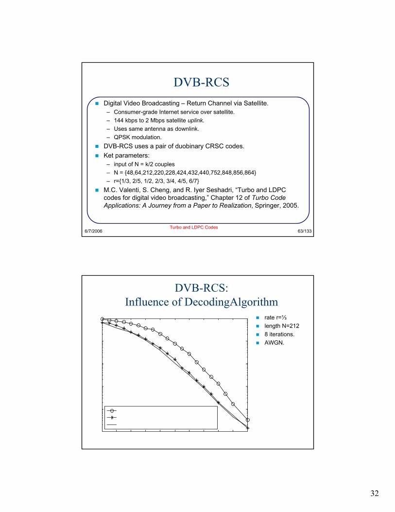
DVB-RCSDigital Video Broadcasting – Return Channel via Satellite.– Consumer-grade Internet service over satellite.– 144 kbps to 2 Mbps satellite uplink.– Uses same antenna as downlink.– QPSK modulation.

DVB-RCS uses a pair of duobinary CRSC codes.Ket parameters:– input of N = k/2 couples– N = {48,64,212,220,228,424,432,440,752,848,856,864}– r={1/3, 2/5, 1/2, 2/3, 3/4, 4/5, 6/7}

M.C. Valenti, S. Cheng, and R. Iyer Seshadri, “Turbo and LDPC codes for digital video broadcasting,” Chapter 12 of Turbo Code Applications: A Journey from a Paper to Realization, Springer, 2005.

DVB-RCS: Influence of DecodingAlgorithm

rate r=⅓length N=2128 iterations.AWGN.

33

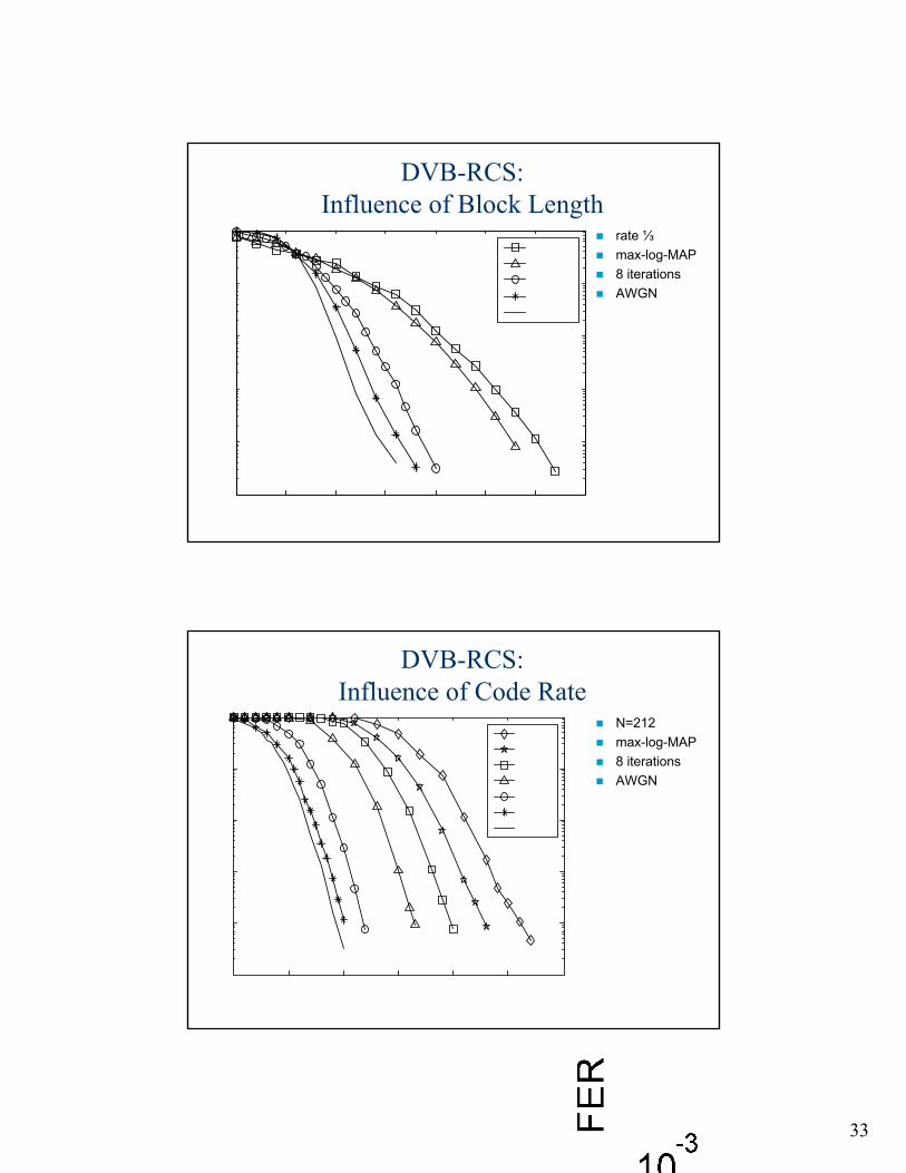
DVB-RCS:Influence of Block Length

rate ⅓max-log-MAP8 iterationsAWGN

DVB-RCS:Influence of Code Rate

N=212max-log-MAP8 iterationsAWGN

34


67/133

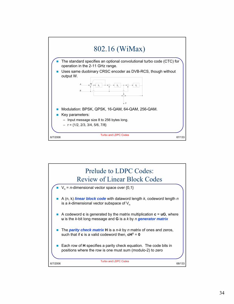
802.16 (WiMax)The standard specifies an optional convolutional turbo code (CTC) for operation in the 2-11 GHz range.Uses same duobinary CRSC encoder as DVB-RCS, though without output W.

Modulation: BPSK, QPSK, 16-QAM, 64-QAM, 256-QAM.Key parameters:– Input message size 8 to 256 bytes long.– r = {1/2, 2/3, 3/4, 5/6, 7/8}

1S 2S 3S

Y

A

B


68/133

Prelude to LDPC Codes:Review of Linear Block Codes

Vn = n-dimensional vector space over {0,1}

A (n, k) linear block code with dataword length k, codeword length nis a k-dimensional vector subspace of Vn

A codeword c is generated by the matrix multiplication c = uG, where u is the k-bit long message and G is a k by n generator matrix

The parity check matrix H is a n-k by n matrix of ones and zeros, such that if c is a valid codeword then, cHT = 0

Each row of H specifies a parity check equation. The code bits in positions where the row is one must sum (modulo-2) to zero

35


69/133

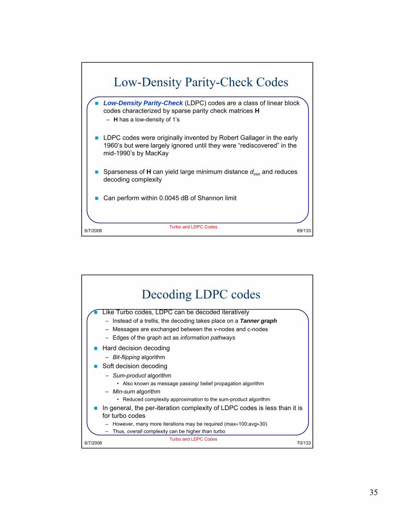
Low-Density Parity-Check CodesLow-Density Parity-Check (LDPC) codes are a class of linear block codes characterized by sparse parity check matrices H– H has a low-density of 1’s

LDPC codes were originally invented by Robert Gallager in the early 1960’s but were largely ignored until they were “rediscovered” in the mid-1990’s by MacKay

Sparseness of H can yield large minimum distance dmin and reduces decoding complexity

Can perform within 0.0045 dB of Shannon limit


70/133

Decoding LDPC codesLike Turbo codes, LDPC can be decoded iteratively– Instead of a trellis, the decoding takes place on a Tanner graph– Messages are exchanged between the v-nodes and c-nodes– Edges of the graph act as information pathways

Hard decision decoding– Bit-flipping algorithm

Soft decision decoding– Sum-product algorithm

• Also known as message passing/ belief propagation algorithm– Min-sum algorithm

• Reduced complexity approximation to the sum-product algorithm

In general, the per-iteration complexity of LDPC codes is less than it is for turbo codes

– However, many more iterations may be required (max≈100;avg≈30)– Thus, overall complexity can be higher than turbo

36


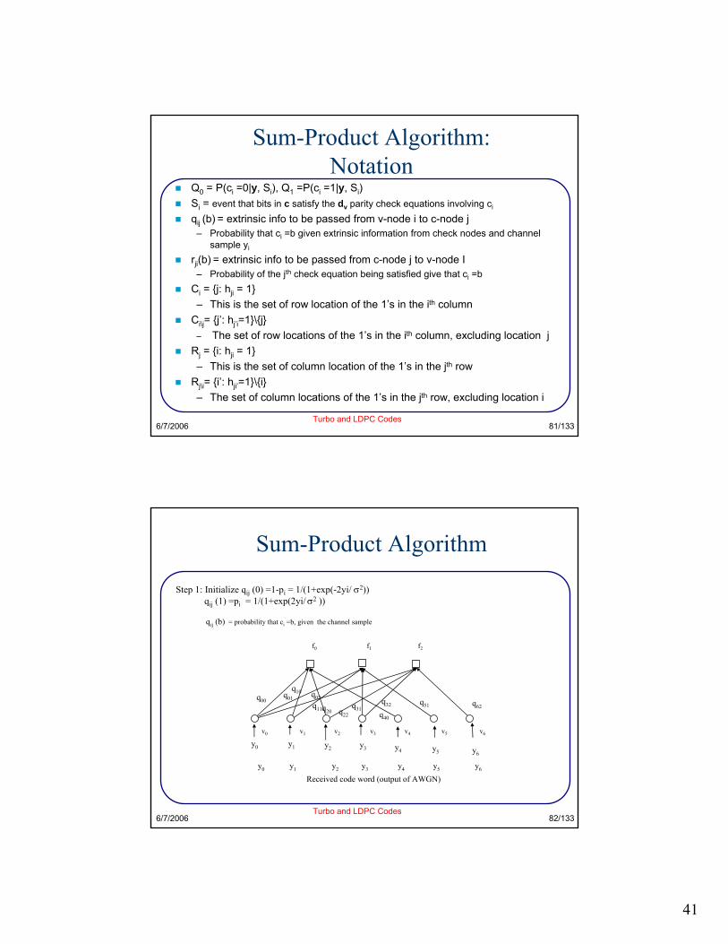
71/133

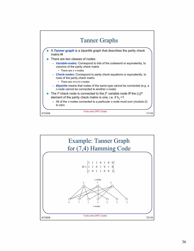
Tanner GraphsA Tanner graph is a bipartite graph that describes the parity check matrix HThere are two classes of nodes:– Variable-nodes: Correspond to bits of the codeword or equivalently, to

columns of the parity check matrix• There are n v-nodes

– Check-nodes: Correspond to parity check equations or equivalently, to rows of the parity check matrix

• There are m=n-k c-nodes– Bipartite means that nodes of the same type cannot be connected (e.g. a

c-node cannot be connected to another c-node)The ith check node is connected to the jth variable node iff the (i,j)th

element of the parity check matrix is one, i.e. if hij =1– All of the v-nodes connected to a particular c-node must sum (modulo-2)

to zero


72/133

Example: Tanner Graphfor (7,4) Hamming Code

⎥⎥⎥

⎦

⎤

⎢⎢⎢

⎣

⎡=

100110101010110010111

H

f0 f1 f2

v0 v1 v2 v3 v4 v5 v6

v-nodes

c-nodes

37


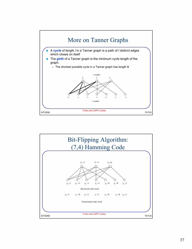
73/133

More on Tanner GraphsA cycle of length l in a Tanner graph is a path of l distinct edges which closes on itselfThe girth of a Tanner graph is the minimum cycle length of the graph.– The shortest possible cycle in a Tanner graph has length 4

f0 f1 f2

v0 v1 v2 v3 v4 v5 v6

v-nodes

c-nodes


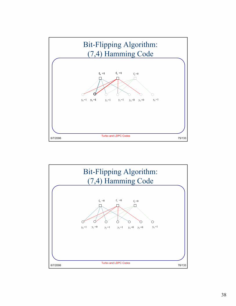
74/133

Bit-Flipping Algorithm:(7,4) Hamming Code

f1 =1

y0 =1 y1 =1 y2 =1 y3 =1 y4 =0 y5 =0 y6 =1

c0 =1 c1 =0 c2 =1 c3 =1 c4 =0 c5 =0 c6 =1

f2 =0

Transmitted code word

Received code word

f0 =1

38


75/133


y0 =1 y2 =1 y3 =1 y6 =1y4 =0 y5 =0y1 =1

f2 =0f0 =1 f1 =1


76/133


y0 =1 y2 =1 y3 =1 y6 =1y4 =0 y5 =0y1 =0

f2 =0f0 =0 f1 =0

39


77/133

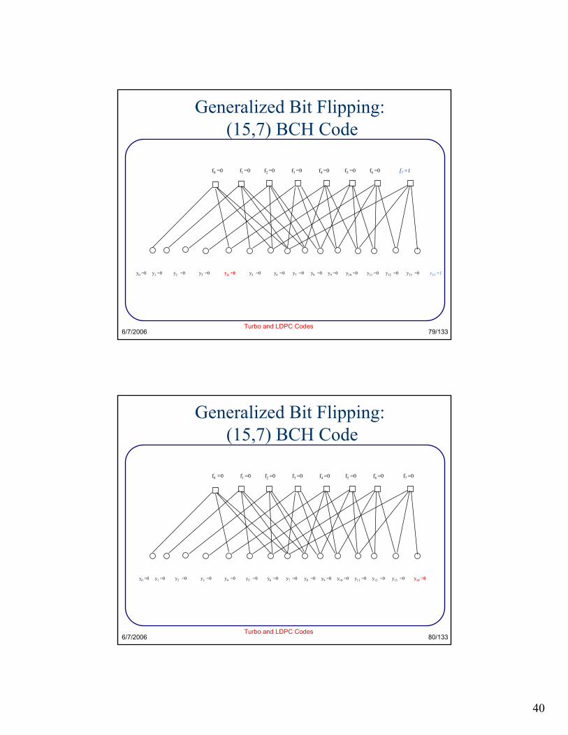
Generalized Bit-Flipping Algorithm

Step 1: Compute parity-checks– If all checks are zero, stop decoding

Step 2: Flip any digit contained in T or more failed check equations

Step 3: Repeat 1 to 2 until all the parity checks are zero or a maximum number of iterations are reached

The parameter T can be varied for a faster convergence


78/133

Generalized Bit Flipping:(15,7) BCH Code

f0 =1 f1 =0 f2 =0 f3 =0 f4 =1 f5 =0 f6 =0 f7 =1

Transmitted code word

c0 =0 c1 =0 c2 =0 c3 =0 c4 =0 c5 =0 c6 =0 c7 =0 c8 =0 c9 =0 c10 =0 c11 =0 c12 =0 c13 =0 c14 =0

y0 =0 y1 =0 y2 =0 y3 =0 y4 =1 y5 =0 y6 =0 y7 =0 y8 =0 y9 =0 y10 =0 y11 =0 y12 =0 y13 =0 y14 =1

Received code word

40


79/133


f0 =0 f1 =0 f2 =0 f3 =0 f4 =0 f5 =0 f6 =0 f7 =1



80/133


f0 =0 f1 =0 f2 =0 f3 =0 f4 =0 f5 =0 f6 =0 f7 =0


41


81/133

Sum-Product Algorithm:Notation

Q0 = P(ci =0|y, Si), Q1 =P(ci =1|y, Si)Si = event that bits in c satisfy the dv parity check equations involving ci

qij (b) = extrinsic info to be passed from v-node i to c-node j– Probability that ci =b given extrinsic information from check nodes and channel

sample yi

rji(b) = extrinsic info to be passed from c-node j to v-node I– Probability of the jth check equation being satisfied give that ci =b

Ci = {j: hji = 1} – This is the set of row location of the 1’s in the ith column

Ci\j= {j’: hj’i=1}\{j}– The set of row locations of the 1’s in the ith column, excluding location j

Rj = {i: hji = 1} – This is the set of column location of the 1’s in the jth row

Rj\i= {i’: hji’=1}\{i}– The set of column locations of the 1’s in the jth row, excluding location i


82/133

Sum-Product Algorithm

Step 1: Initialize qij (0) =1-pi = 1/(1+exp(-2yi/ σ2))qij (1) =pi = 1/(1+exp(2yi/ σ2 ))

Received code word (output of AWGN)y0 y1 y2 y3 y4 y5 y6

f0 f1 f2

v0 v1 v2 v3 v4 v5 v6

y0 y1 y2 y3 y4 y5 y6

q00q01 q02

q10

q22

q32

q40

q62q11q20q31

q51

qij (b) = probability that ci =b, given the channel sample

42


83/133

Sum-Product Algorithm

f0

v0 v1 v2 v3 v4 v5 v6

f1

r23

Step 2: At each c-node, update the r messages ( )\

''

1 1(0) 1 2 (1)2 2

(1) 1 (0)j i

ji i ji R

ji ji

r q

r r∈

= + −

= −

∏

r00 r01

r02 r03r26

f2

r22r20r10

r11

r13

r15

rji (b) = probability that jth check equation is satisfied given ci =b


84/133

Sum-Product Algorithm( )

( )\

\

''

''

(0) (1 ) (0)

(1) ( ) (1)i j

i j

ij ij i j ij C

ij ij i j ij C

q k p r

q k p r

∈

∈

= −

=

∏

∏

( )

( )

(0) (1 ) (0)

(1) ( ) (1)i

i

i ij i jij C

i ij i jij C

Q k p r

Q k p r∈

∈

= −

=

∏

∏

Step 3: Update qij (0) and qij (1)

f0 f1 f2

v0 v1 v2 v3 v4 v5 v6

y0 y1 y2 y3 y4 y5 y6

q00 q01q02

Make hard decision

1 if (1) 0.5ˆ

0 otherwisei

i

Qc

≥⎧= ⎨

⎩

q10q62q51q40q31

q32

q20 q22q11

43


85/133

Halting CriteriaAfter each iteration, halt if:

This is effective, because the probability of an undetectable decoding error is negligible

Otherwise, halt once the maximum number of iterations is reached

If the Tanner graph contains no cycles, then Qi converges to the true APP value as the number of iterations tends to infinity

0Hc =Tˆ


86/133

Sum-Product Algorithm in Log Domain

The sum-product algorithm in probability domain has two shortcomings– Numerically unstable – Too many multiplications

A log domain version is often used for practical purposes

LLR of the ith code bit (ultimate goal of algorithm)

qij = log (qij(0)/qij(1))extrinsic info to be passed from v-node i to c-node j

rji = log(rji(0)/rji(1))extrinsic info to be passed from c-node j to v-node I

( 0 | , )log

( 1| , )i i

ii i

P c y SQ

P c y S⎛ ⎞=

= ⎜ ⎟⎜ ⎟=⎝ ⎠

44


87/133

Sum-Product Decoder (in Log-Domain)

Initialize:– qij = λi = 2yi/σ2 = channel LLR value

Loop over all i,j for which hij = 1– At each c-node, update the r messages:

– At each v-node update the q message and Q LLR:

– Make hard decision:

( )⎟⎟⎠

⎞⎜⎜⎝

⎛⎟⎟⎠

⎞⎜⎜⎝

⎛= ∑∏

∈∈ ijij Riji

Rijijir

\\ ''

'' βφφα

jiiij

Cjjiii

rQq

rQi

−=

+= ∑∈

λ

⎩⎨⎧ <

=otherwise0

0 if1ˆ i

i

Qc


88/133

Sum-Product Algorithm:Notation

αij = sign( qij )βij = | qij |φ(x) = -log tanh(x/2) = log( (ex+1)/(ex-1) )= φ-1(x)

0 1 2 3 4 5 60

1

2

3

4

5

6

x

φ(x)

45


89/133

Min-Sum AlgorithmNote that:

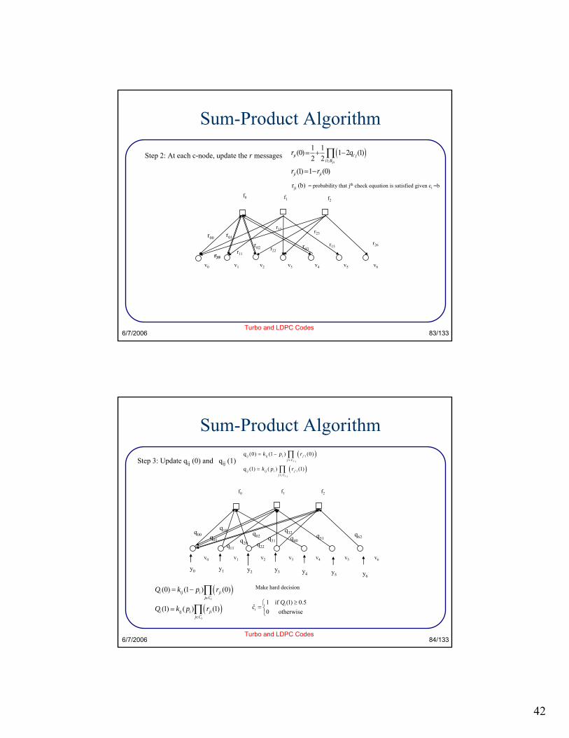
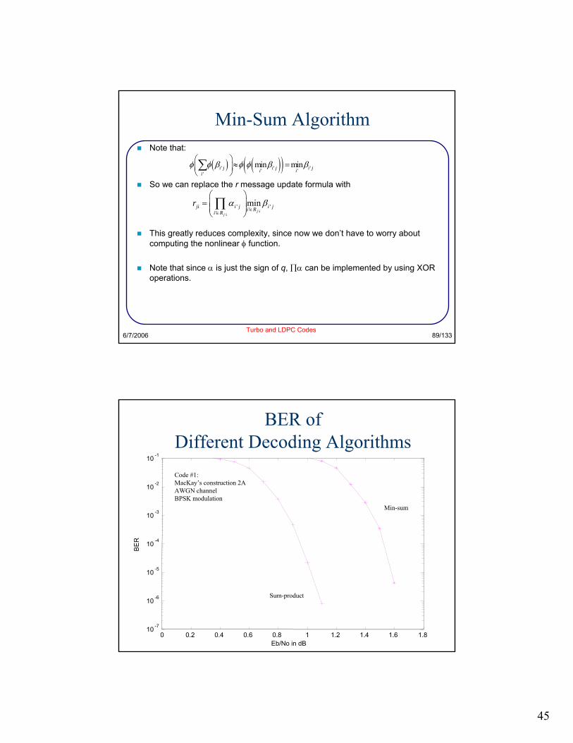
So we can replace the r message update formula with

This greatly reduces complexity, since now we don’t have to worry about computing the nonlinear φ function.

Note that since α is just the sign of q, ∏α can be implemented by using XOR operations.

( ) ( )( )' ' '' ''

min mini j i j i ji ii

φ φ β φ φ β β⎛ ⎞ ≈ =⎜ ⎟⎝ ⎠∑

\\

' '''

minj i

j i

ji i j i ji Ri R

r α β∈

∈

⎛ ⎞= ⎜ ⎟⎜ ⎟

⎝ ⎠∏

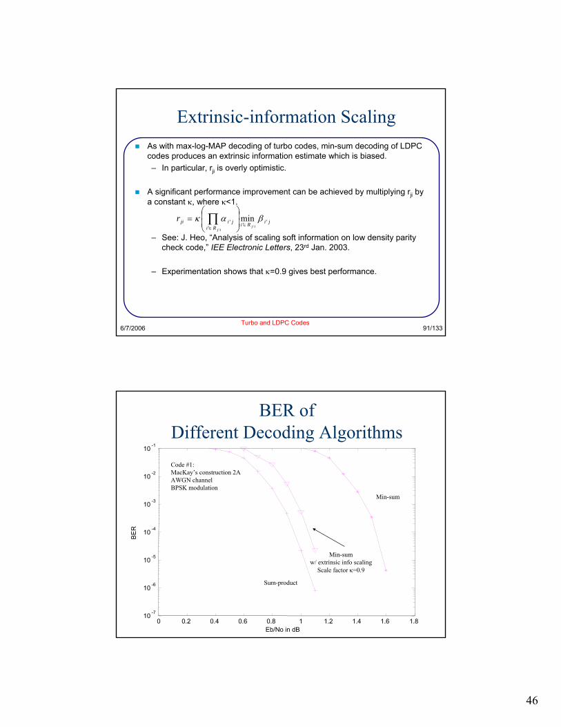
BER of Different Decoding Algorithms

0 0.2 0.4 0.6 0.8 1 1.2 1.4 1.6 1.810 -7

10 -6

10 -5

10 -4

10 -3

10 -2

10 -1

Eb/No in dB

BE

R

Min-sum

Sum-product

Code #1:MacKay’s construction 2AAWGN channelBPSK modulation

46


91/133

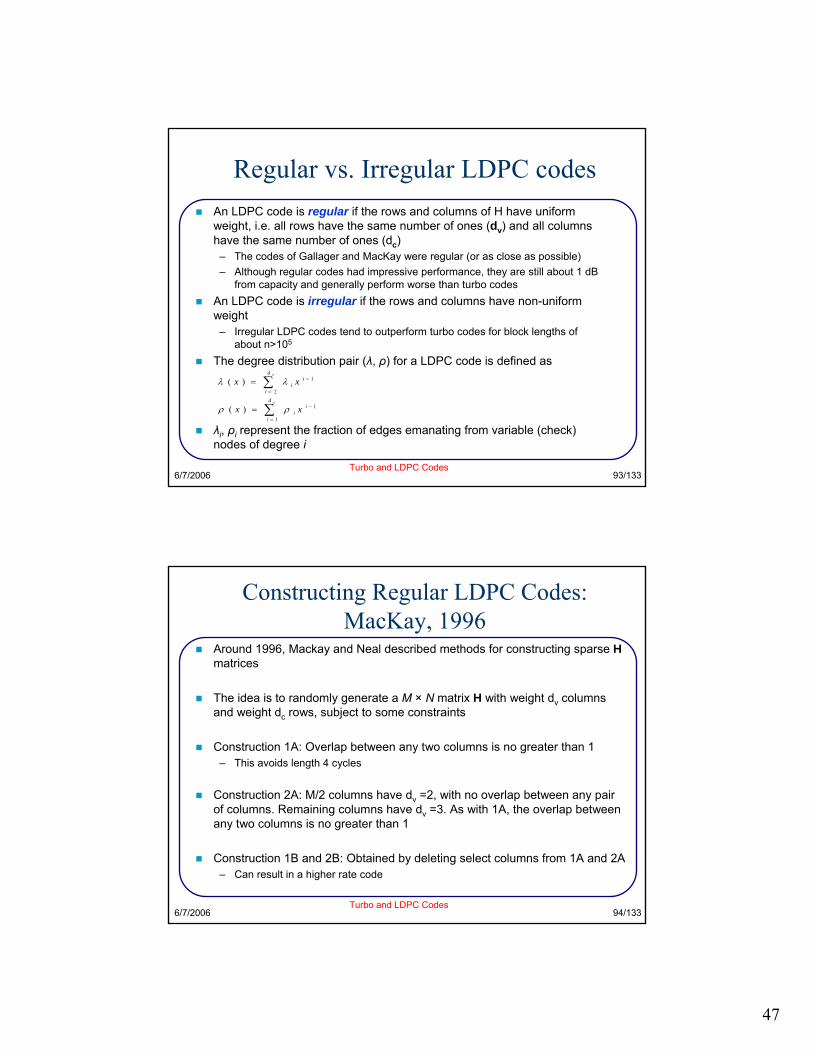
Extrinsic-information ScalingAs with max-log-MAP decoding of turbo codes, min-sum decoding of LDPC codes produces an extrinsic information estimate which is biased.– In particular, rji is overly optimistic.

A significant performance improvement can be achieved by multiplying rji by a constant κ, where κ<1.

– See: J. Heo, “Analysis of scaling soft information on low density parity check code,” IEE Electronic Letters, 23rd Jan. 2003.

– Experimentation shows that κ=0.9 gives best performance.

jiRiRijiji

ijij

r ''''

\\

min βακ∈

∈⎟⎟⎠

⎞⎜⎜⎝

⎛= ∏

BER of Different Decoding Algorithms

0 0.2 0.4 0.6 0.8 1 1.2 1.4 1.6 1.810 -7

10 -6

10 -5

10 -4

10 -3

10 -2

10 -1

Eb/No in dB

BE

R

Min-sum

Min-sumw/ extrinsic info scaling

Scale factor κ=0.9

Sum-product

Code #1:MacKay’s construction 2AAWGN channelBPSK modulation

47


93/133

Regular vs. Irregular LDPC codesAn LDPC code is regular if the rows and columns of H have uniform weight, i.e. all rows have the same number of ones (dv) and all columns have the same number of ones (dc)

– The codes of Gallager and MacKay were regular (or as close as possible)– Although regular codes had impressive performance, they are still about 1 dB

from capacity and generally perform worse than turbo codesAn LDPC code is irregular if the rows and columns have non-uniform weight

– Irregular LDPC codes tend to outperform turbo codes for block lengths of about n>105

The degree distribution pair (λ, ρ) for a LDPC code is defined as

λi, ρi represent the fraction of edges emanating from variable (check)nodes of degree i

1

2

1

1

( )

( )

v

c

di

ii

di

ii

x x

x x

λ λ

ρ ρ

−

=

−

=

=

=

∑

∑


94/133

Constructing Regular LDPC Codes:MacKay, 1996

Around 1996, Mackay and Neal described methods for constructing sparse Hmatrices

The idea is to randomly generate a M × N matrix H with weight dv columns and weight dc rows, subject to some constraints

Construction 1A: Overlap between any two columns is no greater than 1– This avoids length 4 cycles

Construction 2A: M/2 columns have dv =2, with no overlap between any pair of columns. Remaining columns have dv =3. As with 1A, the overlap between any two columns is no greater than 1

Construction 1B and 2B: Obtained by deleting select columns from 1A and 2A– Can result in a higher rate code

48


95/133

Constructing Irregular LDPC Codes:Luby, et. al., 1998

Luby et. al. (1998) developed LDPC codes based on irregular LDPC Tanner graphsMessage and check nodes have conflicting requirements– Message nodes benefit from having a large degree– LDPC codes perform better with check nodes having low degrees

Irregular LDPC codes help balance these competing requirements– High degree message nodes converge to the correct value quickly– This increases the quality of information passed to the check nodes,

which in turn helps the lower degree message nodes to convergeCheck node degree kept as uniform as possible and variable node degree is non-uniform– Code 14: Check node degree =14, Variable node degree =5, 6, 21, 23

No attempt made to optimize the degree distribution for a given code rate


96/133

Density Evolution:Richardson and Urbanke, 2001

Given an irregular Tanner graph with a maximum dv and dc, what is the best degree distribution?

– How many of the v-nodes should be degree dv, dv-1, dv-2,... nodes?– How many of the c-nodes should be degree dc, dc-1,.. nodes?

Question answered using Density Evolution– Process of tracking the evolution of the message distribution during belief

propagation

For any LDPC code, there is a “worst case” channel parameter called the threshold such that the message distribution during belief propagation evolves in such a way that the probability of error converges to zero as the number of iterations tends to infinity

Density evolution is used to find the degree distribution pair (λ, ρ) that maximizes this threshold

49


97/133

Density Evolution:Richardson and Urbanke, 2001

Step 1: Fix a maximum number of iterations

Step 2: For an initial degree distribution, find the threshold

Step 3: Apply a small change to the degree distribution– If the new threshold is larger, fix this as the current distribution

Repeat Steps 2-3

Richardson and Urbanke identify a rate ½ code with degree distribution pair which is 0.06 dB away from capacity

– “Design of capacity-approaching irregular low-density parity-check codes”, IEEE Trans. Inf. Theory, Feb. 2001

Chung et.al., use density evolution to design a rate ½ code which is 0.0045dB away from capacity

– “On the design of low-density parity-check codes within 0.0045 dB of the Shannon limit”, IEEE Comm. Letters, Feb. 2001


98/133

More on Code ConstructionLDPC codes, especially irregular codes exhibit error floors at high SNRsThe error floor is influenced by dmin

– Directly designing codes for large dmin is not computationally feasibleRemoving short cycles indirectly increases dmin (girth conditioning)

– Not all short cycles cause error floorsTrapping sets and Stopping sets have a more direct influence on the error floorError floors can be mitigated by increasing the size of minimum stopping sets

– Tian,et. al., “Construction of irregular LDPC codes with low error floors”, in Proc. ICC, 2003

Trapping sets can be mitigated using averaged belief propagation decoding– Milenkovic, “Algorithmic and combinatorial analysis of trapping sets in structured

LDPC codes”, in Proc. Intl. Conf. on Wireless Ntw., Communications and Mobile computing, 2005

LDPC codes based on projective geometry reported to have very low error floors

– Kou, “Low-density parity-check codes based on finite geometries: a rediscovery and new results”, IEEE Tans. Inf. Theory, Nov.1998

50


99/133

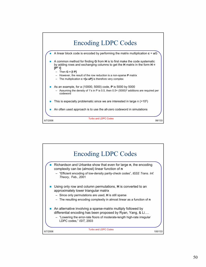
Encoding LDPC CodesA linear block code is encoded by performing the matrix multiplication c = uG

A common method for finding G from H is to first make the code systematic by adding rows and exchanging columns to get the H matrix in the form H = [PT I]

– Then G = [I P]– However, the result of the row reduction is a non-sparse P matrix– The multiplication c =[u uP] is therefore very complex

As an example, for a (10000, 5000) code, P is 5000 by 5000– Assuming the density of 1’s in P is 0.5, then 0.5× (5000)2 additions are required per

codeword

This is especially problematic since we are interested in large n (>105)

An often used approach is to use the all-zero codeword in simulations


100/133

Encoding LDPC CodesRichardson and Urbanke show that even for large n, the encoding complexity can be (almost) linear function of n– “Efficient encoding of low-density parity-check codes”, IEEE Trans. Inf.

Theory, Feb., 2001

Using only row and column permutations, H is converted to an approximately lower triangular matrix – Since only permutations are used, H is still sparse– The resulting encoding complexity in almost linear as a function of n

An alternative involving a sparse-matrix multiply followed by differential encoding has been proposed by Ryan, Yang, & Li…. – “Lowering the error-rate floors of moderate-length high-rate irregular

LDPC codes,” ISIT, 2003

51


101/133

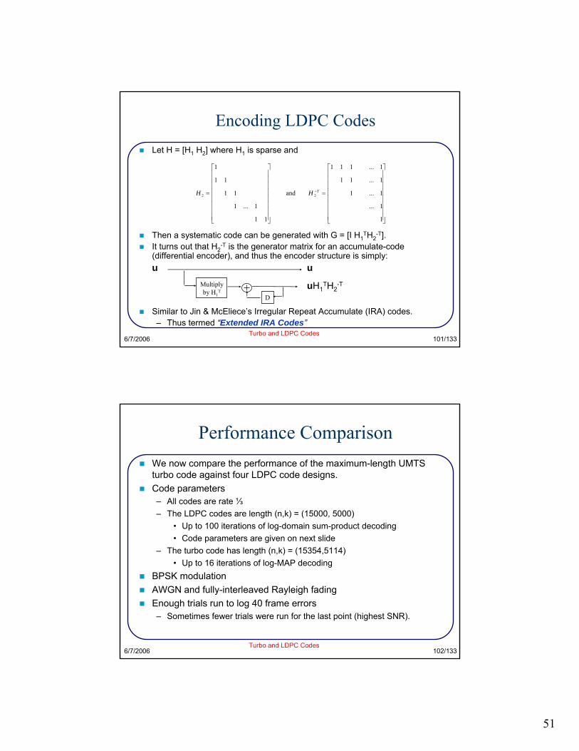
Encoding LDPC CodesLet H = [H1 H2] where H1 is sparse and

Then a systematic code can be generated with G = [I H1TH2

-T].It turns out that H2

-T is the generator matrix for an accumulate-code (differential encoder), and thus the encoder structure is simply:u u

uH1TH2

-T

Similar to Jin & McEliece’s Irregular Repeat Accumulate (IRA) codes.– Thus termed “Extended IRA Codes”

⎥⎥⎥⎥⎥⎥⎥⎥

⎦

⎤

⎢⎢⎢⎢⎢⎢⎢⎢

⎣

⎡

=

⎥⎥⎥⎥⎥⎥⎥⎥

⎦

⎤

⎢⎢⎢⎢⎢⎢⎢⎢

⎣

⎡

= −

1

1...

1...1

1...11

1...111

and

11

1...1

11

11

1

22THH

Multiplyby H1

T

D


102/133

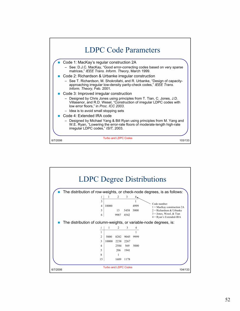
Performance ComparisonWe now compare the performance of the maximum-length UMTS turbo code against four LDPC code designs.Code parameters– All codes are rate ⅓– The LDPC codes are length (n,k) = (15000, 5000)

• Up to 100 iterations of log-domain sum-product decoding• Code parameters are given on next slide

– The turbo code has length (n,k) = (15354,5114)• Up to 16 iterations of log-MAP decoding

BPSK modulationAWGN and fully-interleaved Rayleigh fadingEnough trials run to log 40 frame errors– Sometimes fewer trials were run for the last point (highest SNR).

52


103/133

LDPC Code ParametersCode 1: MacKay’s regular construction 2A– See: D.J.C. MacKay, “Good error-correcting codes based on very sparse

matrices,” IEEE Trans. Inform. Theory, March 1999.Code 2: Richardson & Urbanke irregular construction– See T. Richardson, M. Shokrollahi, and R. Urbanke, “Design of capacity-

approaching irregular low-density parity-check codes,” IEEE Trans. Inform. Theory, Feb. 2001.

Code 3: Improved irregular construction– Designed by Chris Jones using principles from T. Tian, C. Jones, J.D.

Villasenor, and R.D. Wesel, “Construction of irregular LDPC codes with low error floors,” in Proc. ICC 2003.

– Idea is to avoid small stopping setsCode 4: Extended IRA code– Designed by Michael Yang & Bill Ryan using principles from M. Yang and

W.E. Ryan, “Lowering the error-rate floors of moderate-length high-rate irregular LDPC codes,” ISIT, 2003.


104/133

LDPC Degree DistributionsThe distribution of row-weights, or check-node degrees, is as follows:

The distribution of column-weights, or variable-node degrees, is:

454299876500054581354999100004

134321i

117816891518

19412065500056925844

2267223810000399999045828250002

114321i

Code number:1 = MacKay construction 2A2 = Richardson & Urbanke3 = Jones, Wesel, & Tian4 = Ryan’s Extended-IRA

53

BER in AWGN

Code #1:Mackay 2A

Code #4:IRA

Code #2:R&U

Code #3:JWT

turbo

BPSK/AWGN Capacity:-0.50 dB for r = 1/3

0 0.2 0.4 0.6 0.8 1 1.210

-7

10-6

10-5

10-4

10-3

10-2

10-1

Eb/No in dB

BER


106/133

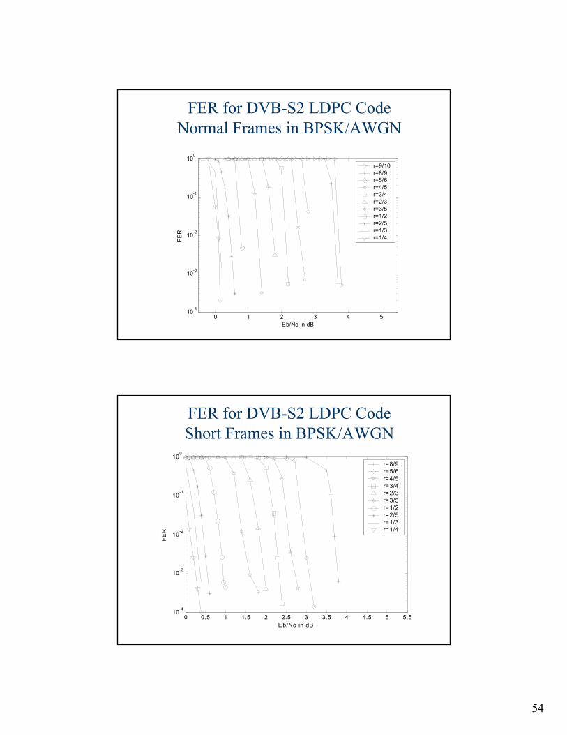
DVB-S2 LDPC CodeThe digital video broadcasting (DVB) project was founded in 1993 by ETSI to standardize digital television services

The latest version of the standard DVB-S2 uses a concatenation of an outer BCH code and inner LDPC code

The codeword length can be either n =64800 (normal frames) or n =16200 (short frames)

Normal frames support code rates 9/10, 8/9, 5/6, 4/5, 3/4, 2/3, 3/5, 1/2, 2/5, 1/3, 1/4

– Short frames do not support rate 9/10DVB-S2 uses an extended-IRA type LDPC code

Valenti, et. al, “Turbo and LDPC codes for digital video broadcasting,” Chapter 12 of Turbo Code Application: A Journey from a Paper to Realizations, Springer, 2005.

54

FER for DVB-S2 LDPC Code Normal Frames in BPSK/AWGN

0 1 2 3 4 510-4

10-3

10-2

10-1

100

Eb/No in dB

FER

r=9/10r=8/9r=5/6r=4/5r=3/4r=2/3r=3/5r=1/2r=2/5r=1/3r=1/4

FER for DVB-S2 LDPC CodeShort Frames in BPSK/AWGN

0 0.5 1 1.5 2 2.5 3 3.5 4 4.5 5 5.510

-4

10-3

10-2

10-1

100

Eb/No in dB

FER

r=8/9r=5/6r=4/5r=3/4r=2/3r=3/5r=1/2r=2/5r=1/3r=1/4

55


109/133

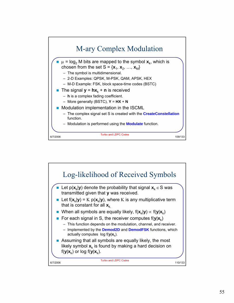
M-ary Complex Modulationµ = log2 M bits are mapped to the symbol xk, which is chosen from the set S = {x1, x2, …, xM}– The symbol is multidimensional.– 2-D Examples: QPSK, M-PSK, QAM, APSK, HEX– M-D Example: FSK, block space-time codes (BSTC)

The signal y = hxk + n is received– h is a complex fading coefficient.– More generally (BSTC), Y = HX + N

Modulation implementation in the ISCML– The complex signal set S is created with the CreateConstellation

function.– Modulation is performed using the Modulate function.


110/133

Log-likelihood of Received SymbolsLet p(xk|y) denote the probability that signal xk ∈S was transmitted given that y was received.Let f(xk|y) = Κ p(xk|y), where Κ is any multiplicative term that is constant for all xk.

When all symbols are equally likely, f(xk|y) ∝ f(y|xk) For each signal in S, the receiver computes f(y|xk)– This function depends on the modulation, channel, and receiver.– Implemented by the Demod2D and DemodFSK functions, which

actually computes log f(y|xk).

Assuming that all symbols are equally likely, the most likely symbol xk is found by making a hard decision on f(y|xk) or log f(y|xk).

56


111/133

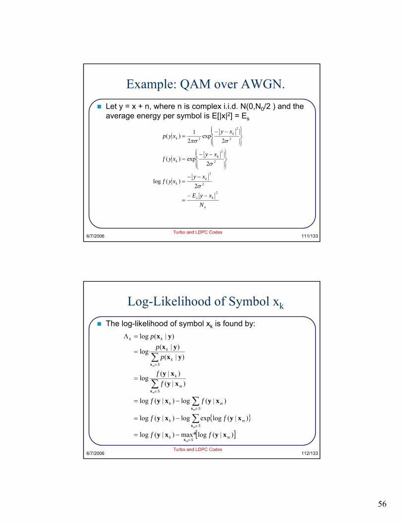
Example: QAM over AWGN.Let y = x + n, where n is complex i.i.d. N(0,N0/2 ) and the average energy per symbol is E[|x|2] = Es

o

ks

kk

kk

kk

NxyE

xyxyf

xyxyf

xyxyp

2

2

2

2

2

2

2

2

2)(log

2exp)(

2exp

21)(

−−=

−−=

⎪⎭

⎪⎬⎫

⎪⎩

⎪⎨⎧ −−

=

⎪⎭

⎪⎬⎫

⎪⎩

⎪⎨⎧ −−

=

σ

σ

σπσ


112/133

Log-Likelihood of Symbol xk

The log-likelihood of symbol xk is found by:

{ }

[ ])|(logmax*)|(log

)|(logexplog)|(log

)|(log)|(log

)|()|(

log

)|()|(

log

)|(log

mSk

Smk

Smk

Sm

k

Sk

k

kk

ff

ff

ff

ff

pp

p

m

m

m

m

m

xyxy

xyxy

xyxy

xyxy

yxyx

yx

x

x

x

x

x

∈

∈

∈

∈

∈

−=

−=

−=

=

=

=Λ

∑

∑

∑

∑

57

The max* function

0 1 2 3 4 5 6 7 8 9 10-0.1

0

0.1

0.2

0.3

0.4

0.5

0.6

0.7

|y-x|

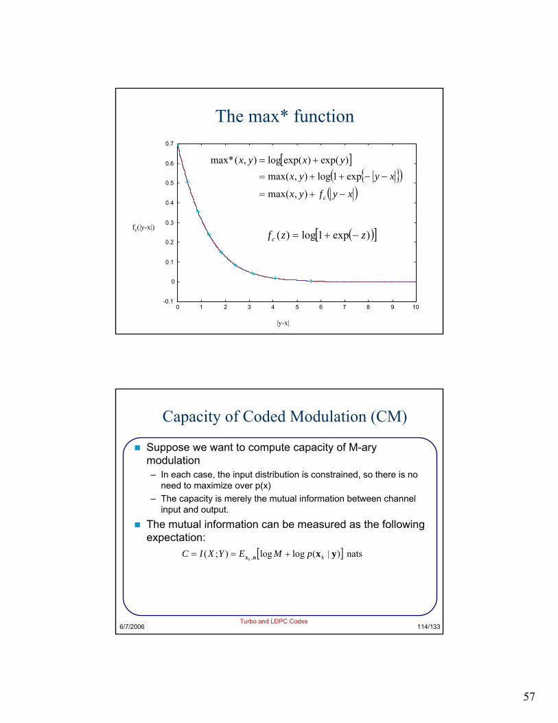
fc(|y-x|) ( )[ ])exp1log)( zzfc −+=

[ ]{ }( )

( )xyfyx

xyyxyxyx

c −+=

−−++=

+=

),max(

exp1log),max()exp()exp(log),(max*


114/133

Capacity of Coded Modulation (CM)

Suppose we want to compute capacity of M-arymodulation – In each case, the input distribution is constrained, so there is no

need to maximize over p(x)– The capacity is merely the mutual information between channel

input and output.

The mutual information can be measured as the following expectation:

[ ] nats )|(loglog);( , yxnx kpMEYXICk

+==

58


115/133

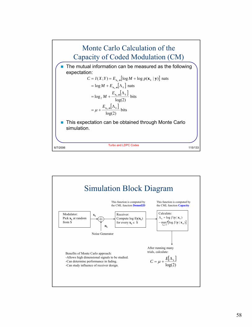
Monte Carlo Calculation of the Capacity of Coded Modulation (CM)

The mutual information can be measured as the following expectation:

This expectation can be obtained through Monte Carlo simulation.

[ ][ ]

[ ]

[ ]bits

log(2)

bits log(2)

log

nats log

nats )|(loglog);(

,

,2

,

,

k

k

k

k

k

k

k

k

E

EM

EM

pMEYXIC

Λ+=

Λ+=

Λ+=

+==

nx

nx

nx

nx yx

µ

Simulation Block Diagram

Modulator:Pick xk at randomfrom S

xk

nk

Noise Generator

Receiver:Compute log f(y|xk)for every xk ∈ S

Calculate:

After running many trials, calculate:

[ ])2log(

kEC

Λ+= µ

Benefits of Monte Carlo approach:-Allows high dimensional signals to be studied.-Can determine performance in fading.-Can study influence of receiver design.

[ ])|(logmax*)|(log

mS

kk

ff

m

xyxy

x ∈−

=Λ

This function is computed by the CML function Capacity

This function is computed by the CML function Demod2D

59

-2 0 2 4 6 8 10 12 14 16 18 200

1

2

3

4

5

6

7

8

Eb/No in dB

Cap

acity

(bits

per

sym

bol)

2-D U

nconst

rained

Capacity

256QAM

64QAM

16QAM

16PSK

8PSK

QPSK

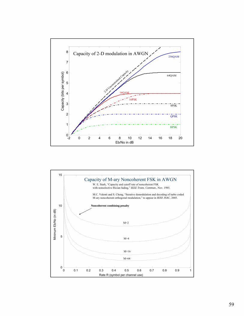
Capacity of 2-D modulation in AWGN

BPSK

Capacity of M-ary Noncoherent FSK in AWGNW. E. Stark, “Capacity and cutoff rate of noncoherent FSKwith nonselective Rician fading,” IEEE Trans. Commun., Nov. 1985.

M.C. Valenti and S. Cheng, “Iterative demodulation and decoding of turbo coded M-ary noncoherent orthogonal modulation,” to appear in IEEE JSAC, 2005.

0 0.1 0.2 0.3 0.4 0.5 0.6 0.7 0.8 0.9 10

5

10

15

Rate R (symbol per channel use)

Min

imum

Eb/

No

(in d

B)

M=2

M=4

M=16

M=64

Noncoherent combining penalty

60

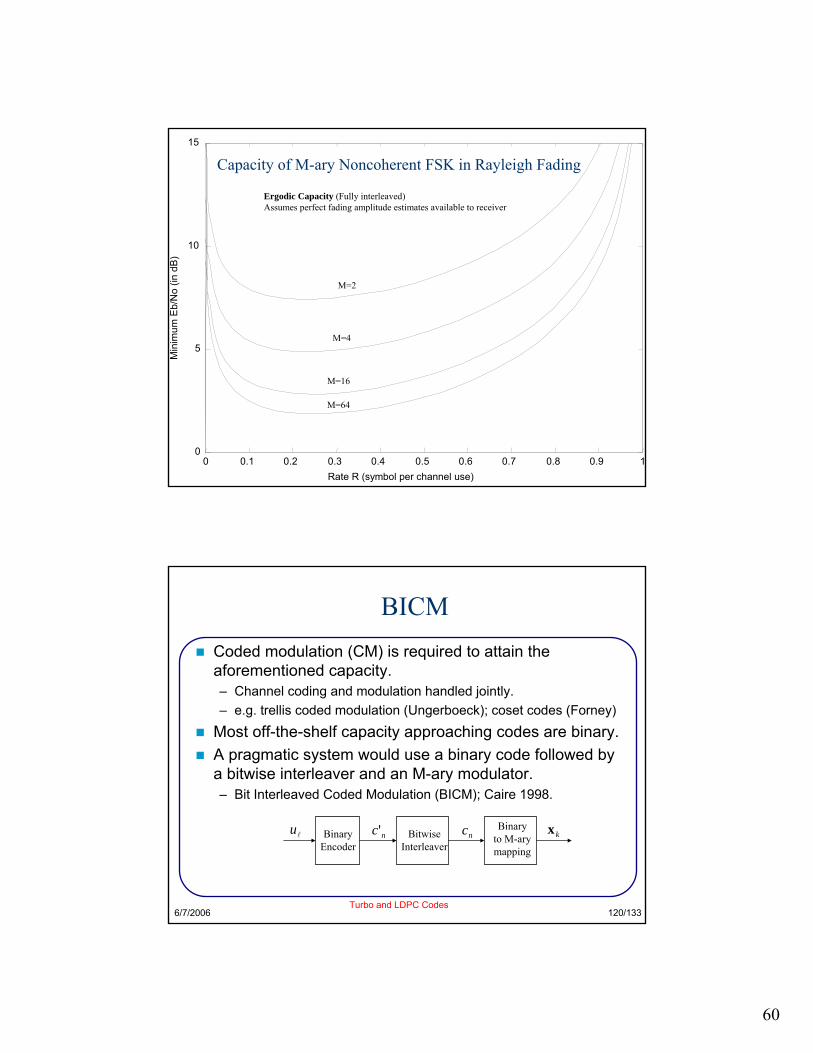
Ergodic Capacity (Fully interleaved)Assumes perfect fading amplitude estimates available to receiver

M=2

M=4

M=16

M=64

0 0.1 0.2 0.3 0.4 0.5 0.6 0.7 0.8 0.9 10

5

10

15

Rate R (symbol per channel use)

Min

imum

Eb/

No

(in d

B)

Capacity of M-ary Noncoherent FSK in Rayleigh Fading


120/133

BICMCoded modulation (CM) is required to attain the aforementioned capacity.– Channel coding and modulation handled jointly.– e.g. trellis coded modulation (Ungerboeck); coset codes (Forney)

Most off-the-shelf capacity approaching codes are binary.A pragmatic system would use a binary code followed by a bitwise interleaver and an M-ary modulator.– Bit Interleaved Coded Modulation (BICM); Caire 1998.

BinaryEncoder

BitwiseInterleaver

Binaryto M-arymapping

lu nc' nc kx

61


121/133

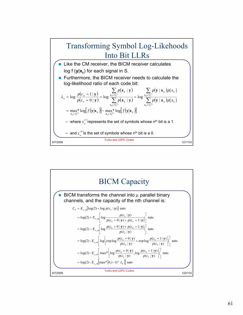
Transforming Symbol Log-LikehoodsInto Bit LLRs

Like the CM receiver, the BICM receiver calculates log f (y|xk) for each signal in S.Furthermore, the BICM receiver needs to calculate the log-likelihood ratio of each code bit:

– where represents the set of symbols whose nth bit is a 1.

– and is the set of symbols whose nth bit is a 0.

( )( )

( )

( )

( )

( )

( )[ ] ( )[ ]kS

kS

Skk

Skk

Sk

Sk

n

nn

ff

xpp

xpp

p

p

cpcp

nknk

nk

nk

nk

nk

xyxy

xy

xy

yx

yx

yy

xx

x

x

x

x

logmax*logmax*

][|

][|log

|

|log

|0|1

log

)0()1(

)0(

)1(

)0(

)1(

∈∈

∈

∈

∈

∈

−=

====

=∑

∑

∑

∑λ

)1(

nS

)0(

nS


122/133

BICM CapacityBICM transforms the channel into µ parallel binary channels, and the capacity of the nth channel is:

[ ]

{ }[ ] nats )1(,0max*-)2log(

nats )|(

)|1(log,

)|()|0(

logmax*-)2log(

nats )|(

)|1(logexp

)|()|0(

logexplog-)2log(

nats )|(

)|1()|0(log)2log(

nats )|1()|0(

)|(log)2log(

nats )|(log)2log(

,

,

,

,

,

,

kc

c

k

k

k

kc

k

k

k

kc

k

kkc

kk

kc

kck

k

n

n

n

n

n

n

E

cpcp

cpcp

E

cpcp

cpcp

E

cpcpcp

E

cpcpcp

E

cpEC

λ−=

⎥⎦

⎤⎢⎣

⎡

⎭⎬⎫

⎩⎨⎧ ==

=

⎥⎦

⎤⎢⎣

⎡

⎭⎬⎫

⎩⎨⎧ =

+=

=

⎥⎦

⎤⎢⎣

⎡ =+=−=

⎥⎦

⎤⎢⎣

⎡=+=

+=

+=

n

n

n

n

n

n

yy

yy

yy

yy

yyy

yyy

y

62


123/133

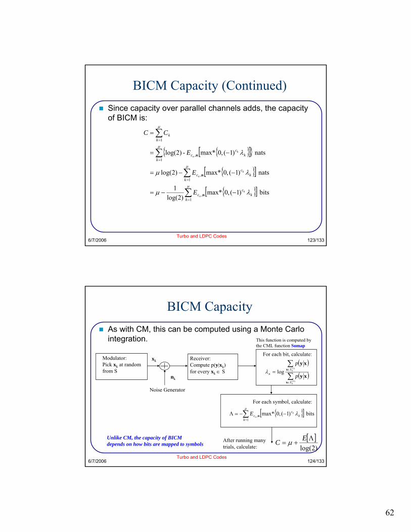
BICM Capacity (Continued)Since capacity over parallel channels adds, the capacity of BICM is:

{ }[ ]{ }

{ }[ ]

{ }[ ] bits )1(,0max*)2log(

1

nats )1(,0max*)2log(

nats )1(,0max*-log(2)

1,

1,

1,

1

∑

∑

∑

∑

=

=

=

=

−−=

−−=

−=

=

µ

µ

µ

µ

λµ

λµ

λ

kk

cc

kk

cc

kk

cc

kk

k

n

k

n

k

n

E

E

E

CC

n

n

n


124/133

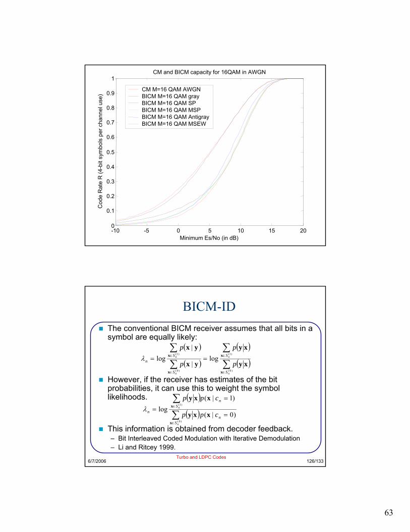
BICM CapacityAs with CM, this can be computed using a Monte Carlo integration.

Modulator:Pick xk at randomfrom S

xk

nk

Noise Generator

Receiver:Compute p(y|xk)for every xk ∈ S

For each bit, calculate:

After running many trials, calculate:

[ ])2log(

Λ+=

EC µUnlike CM, the capacity of BICMdepends on how bits are mapped to symbols

( )

( )∑

∑

∈

∈=

)0(

)1(

log

n

n

S

Sn p

p

x

x

xy

xyλ

For each symbol, calculate:

{ }[ ] bits )1(,0max*1

,∑=

−−=Λµ

λk

kc

ck

nE n

This function is computed by the CML function Somap

63

-10 -5 0 5 10 15 200

0.1

0.2

0.3

0.4

0.5

0.6

0.7

0.8

0.9

1

Cod

e R

ate

R (4

-bit

sym

bols

per

cha

nnel

use

)

Minimum Es/No (in dB)

CM and BICM capacity for 16QAM in AWGN

CM M=16 QAM AWGNBICM M=16 QAM grayBICM M=16 QAM SPBICM M=16 QAM MSPBICM M=16 QAM AntigrayBICM M=16 QAM MSEW


126/133

BICM-IDThe conventional BICM receiver assumes that all bits in a symbol are equally likely:

However, if the receiver has estimates of the bit probabilities, it can use this to weight the symbol likelihoods.

This information is obtained from decoder feedback.– Bit Interleaved Coded Modulation with Iterative Demodulation– Li and Ritcey 1999.

( )

( )

( )

( )∑

∑

∑

∑

∈

∈

∈

∈ ==

)0(

)1(

)0(

)1(

log|

|log

n

n

n

n

S

S

S

Sn p

p

p

p

x

x

x

x

xy

xy

yx

yxλ

( )

( )∑

∑

∈

∈

=

=

=

)0(

)1(

)0|(

)1|(log

n

n

Sn

nS

n cpp

cpp

x

x

xxy

xxyλ

64


127/133

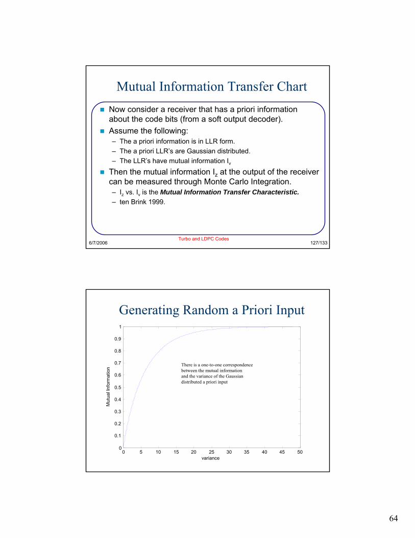
Mutual Information Transfer ChartNow consider a receiver that has a priori information about the code bits (from a soft output decoder).Assume the following:– The a priori information is in LLR form.– The a priori LLR’s are Gaussian distributed.– The LLR’s have mutual information Iv

Then the mutual information Iz at the output of the receiver can be measured through Monte Carlo Integration.– Iz vs. Iv is the Mutual Information Transfer Characteristic.– ten Brink 1999.

Generating Random a Priori Input

0 5 10 15 20 25 30 35 40 45 500

0.1

0.2

0.3

0.4

0.5

0.6

0.7

0.8

0.9

1

variance

Mut

ual I

nfor

mat

ion

There is a one-to-one correspondencebetween the mutual informationand the variance of the Gaussiandistributed a priori input

65

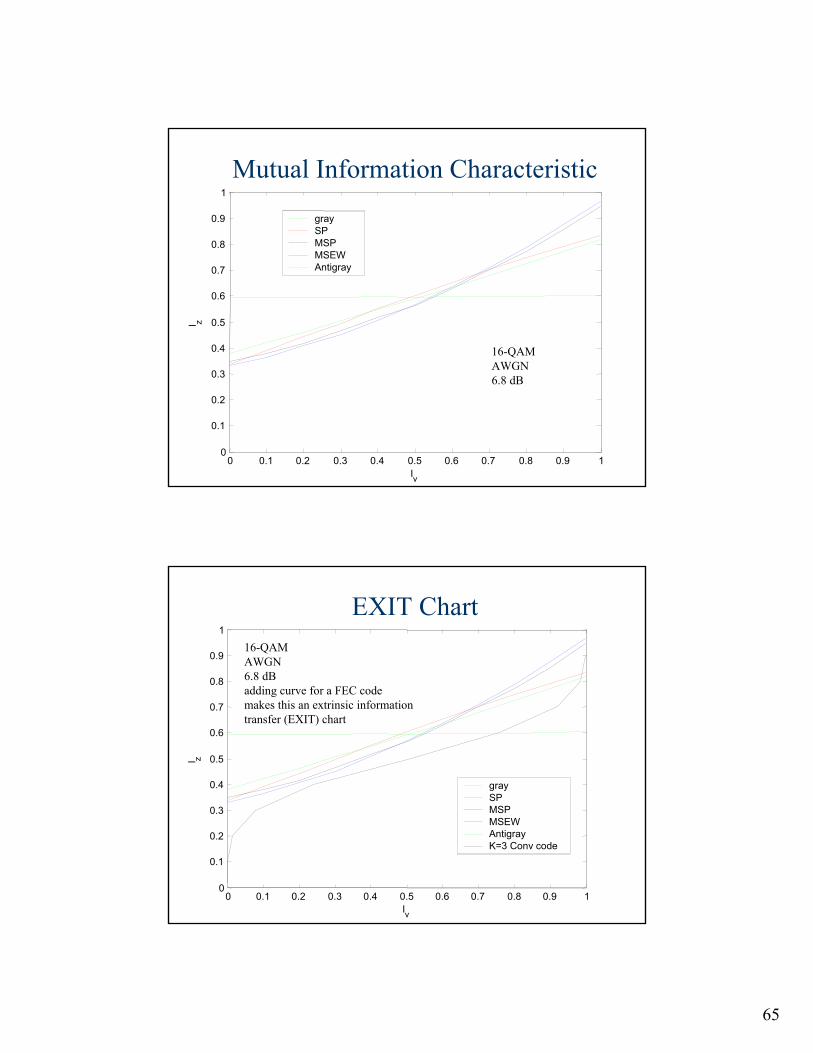
Mutual Information Characteristic

0 0.1 0.2 0.3 0.4 0.5 0.6 0.7 0.8 0.9 10

0.1

0.2

0.3

0.4

0.5

0.6

0.7

0.8

0.9

1

Iv

I z

graySPMSPMSEWAntigray

16-QAMAWGN6.8 dB

EXIT Chart

0 0.1 0.2 0.3 0.4 0.5 0.6 0.7 0.8 0.9 10

0.1

0.2

0.3

0.4

0.5

0.6

0.7

0.8

0.9

1

Iv

I z

graySPMSPMSEWAntigrayK=3 Conv code

16-QAMAWGN6.8 dBadding curve for a FEC codemakes this an extrinsic informationtransfer (EXIT) chart

66

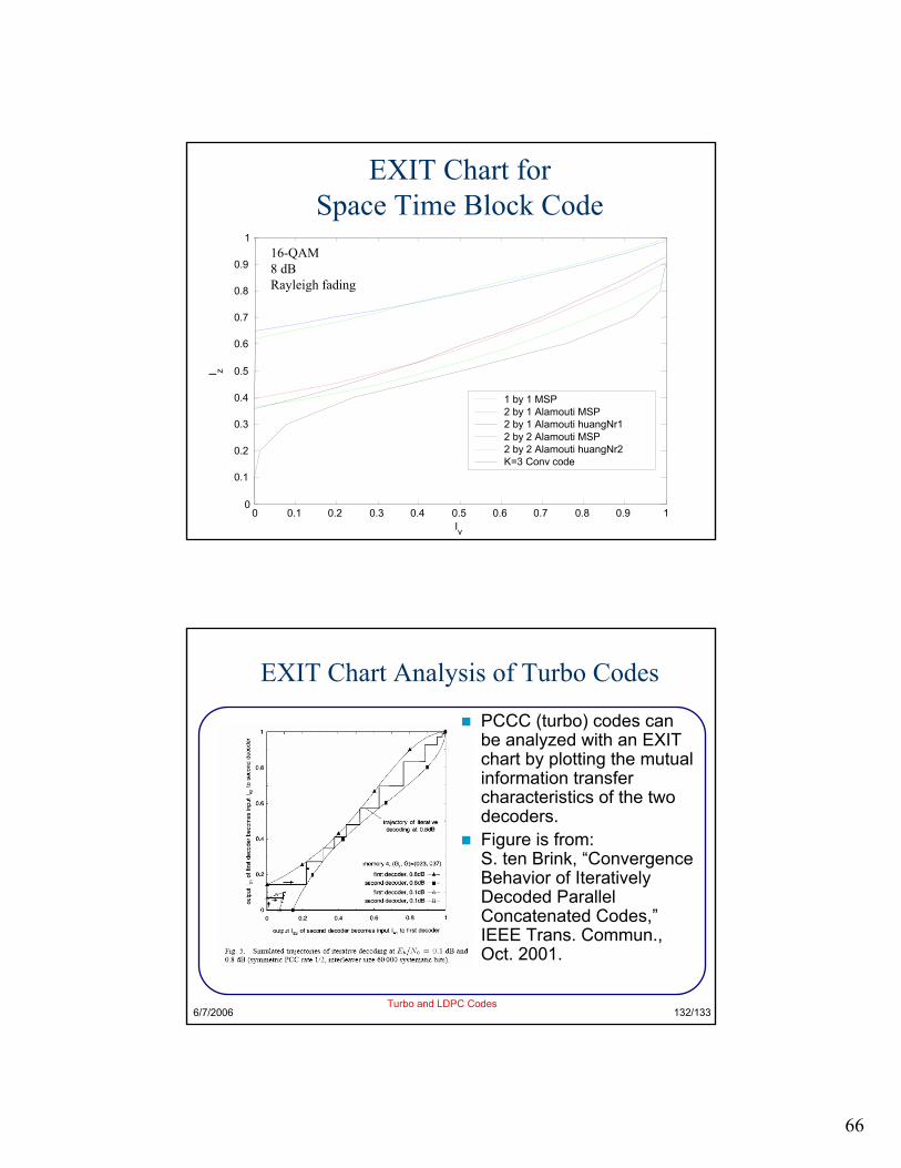
EXIT Chart for Space Time Block Code

0 0.1 0.2 0.3 0.4 0.5 0.6 0.7 0.8 0.9 10

0.1

0.2

0.3

0.4

0.5

0.6

0.7

0.8

0.9

1

Iv

I z

1 by 1 MSP2 by 1 Alamouti MSP2 by 1 Alamouti huangNr12 by 2 Alamouti MSP2 by 2 Alamouti huangNr2K=3 Conv code

16-QAM8 dBRayleigh fading


132/133

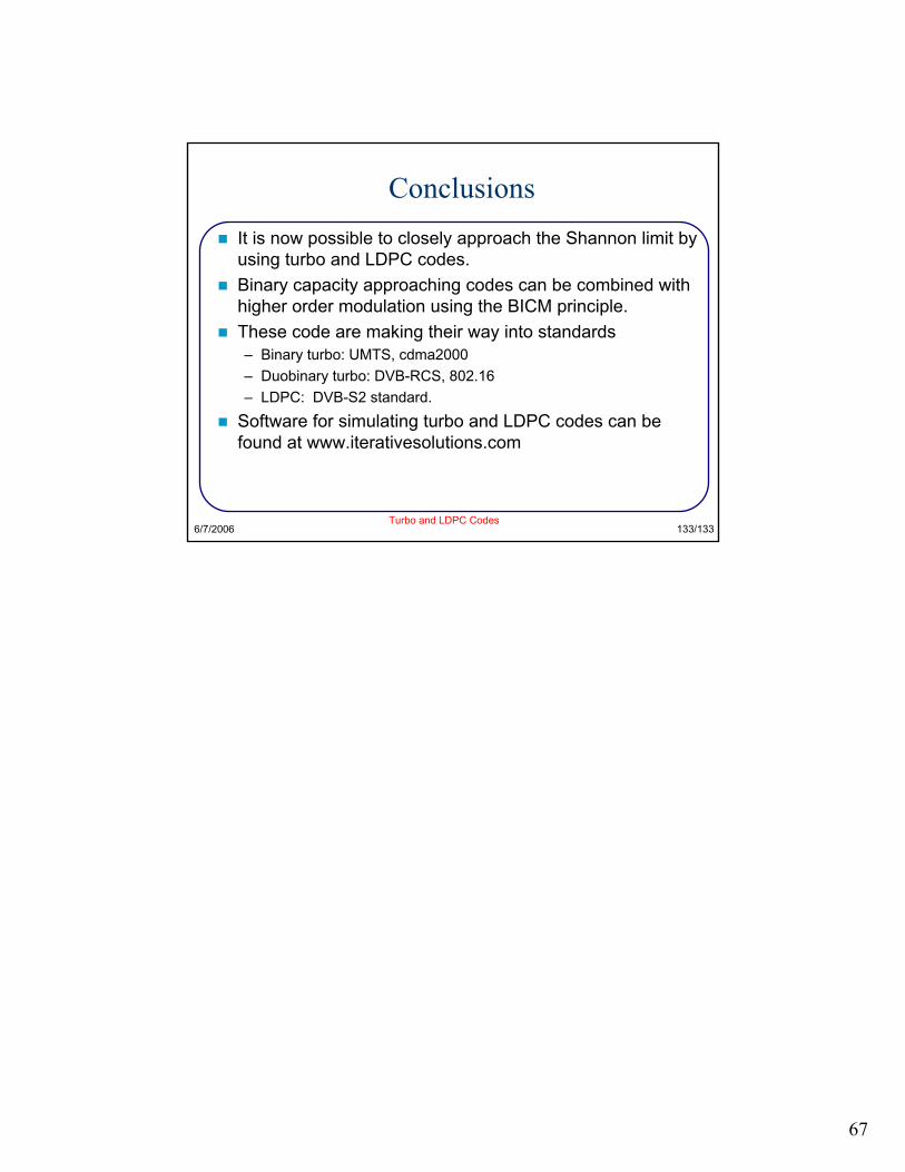
EXIT Chart Analysis of Turbo Codes

PCCC (turbo) codes can be analyzed with an EXIT chart by plotting the mutual information transfer characteristics of the two decoders.Figure is from:S. ten Brink, “Convergence Behavior of Iteratively Decoded Parallel Concatenated Codes,” IEEE Trans. Commun., Oct. 2001.

67


133/133

ConclusionsIt is now possible to closely approach the Shannon limit by using turbo and LDPC codes.Binary capacity approaching codes can be combined with higher order modulation using the BICM principle.These code are making their way into standards– Binary turbo: UMTS, cdma2000 – Duobinary turbo: DVB-RCS, 802.16– LDPC: DVB-S2 standard.

Software for simulating turbo and LDPC codes can be found at www.iterativesolutions.com

Date post:	02-Sep-2019
Category:	Documents
Upload:	others
View:	32 times
Download:	0 times

Turbo and LDPC Codes: Implementation, Simulation, and...

Documents