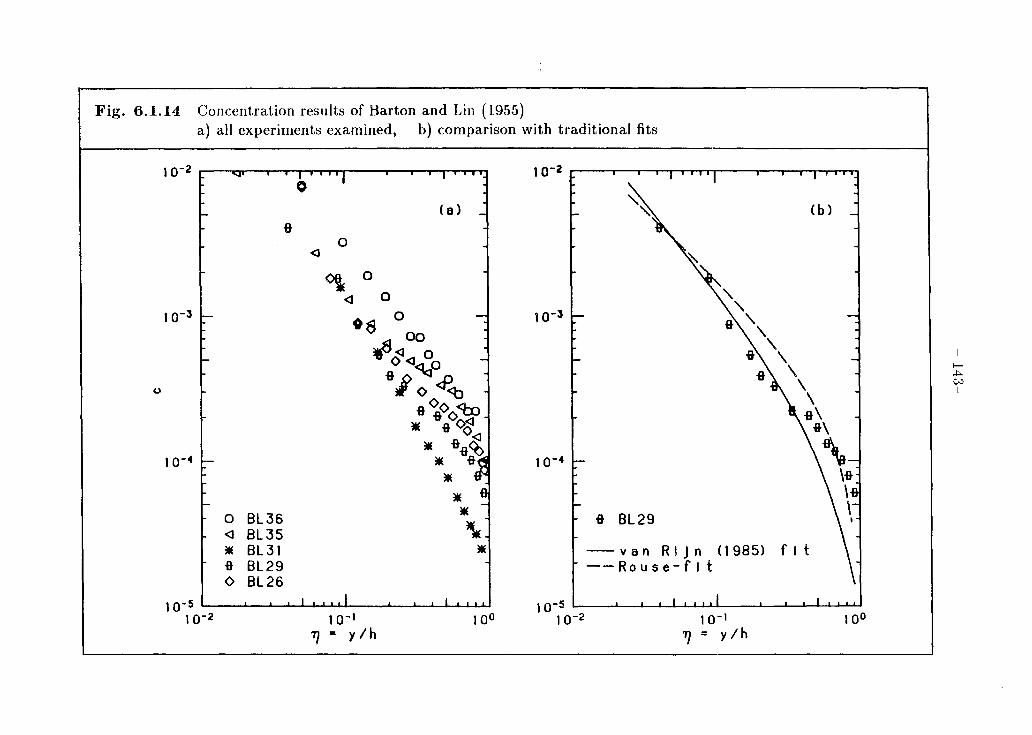
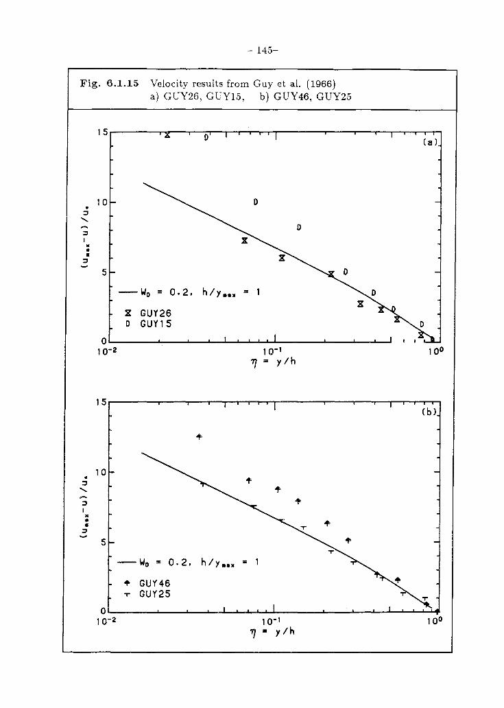
Page 1
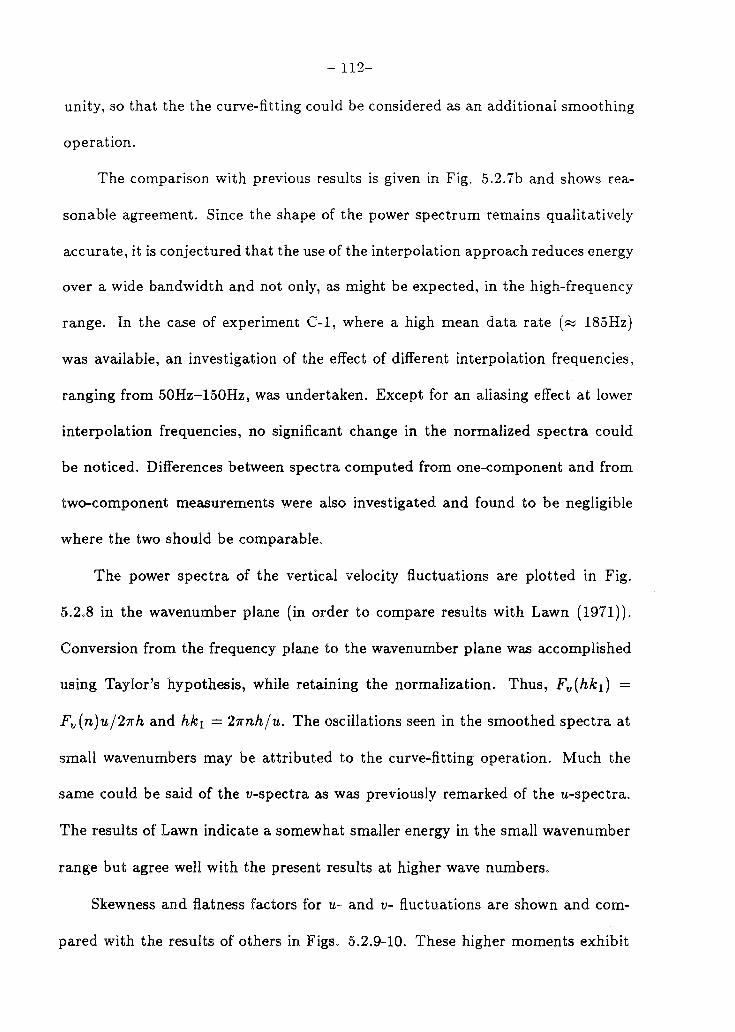
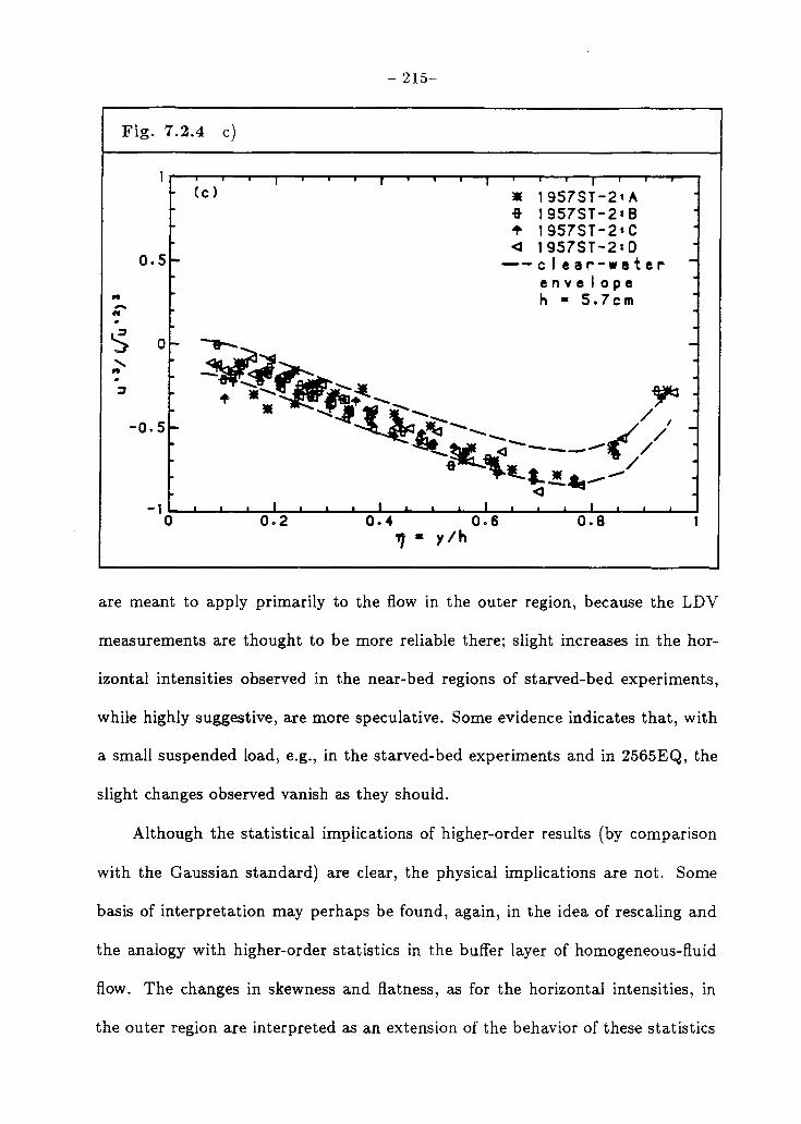
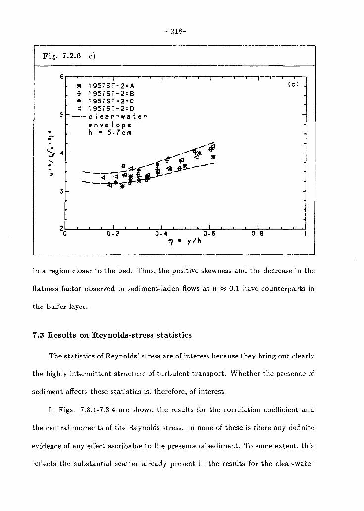
TURBULENCE AND TURBULENT TRANSPORT IN
SEDIMENT-LADEN OPEN-CHANNEL FLOWS
by
Dennis Anthony Lyn
W. M. Keck Laboratory of Hydraulics and Water Resources Division of Engineering and Applied Science
CALIFORNIA INSTITUTE OF TECHNOLOGY
Pasadena, California
Report No. KH-R-49 December 1986
Page 2
Turbulence and Turbulent Transport . In
Sediment-laden
Open-Channel Flows
by
Dennis Anthony Lyn
Project Supervisor:
Norman H. Brooks J ames Irvine Professor of
Environmental and Civil Engineering
Supported by
The National Science Foundation (Grants CEE-7920311, MSM-8611127) James Irvine Professorship
W. M. Keck Laboratory of Hydraulics and Water Resources. Division of Engineering and Applied Science
California Institute of Technology Pasadena, California
Report No. KH-R-49 December 1986
Page 3
- ll-
Copyright ©1986 by Dennis A. Lyn
All rights reserved
Page 4
- 111-
Acknowledgements
A number of people have contributed, directly or indirectly, to the work re
ported here. Prof. N.H. Brooks, my ad visor, suggested the general field of sedi
ment transport as an impossible area of research, instantly seducing the innocent,
and generally allowed me the freedom to go on my own wild goose chases. Vito
Vanoni provided constant encouragement even when he was not, perhaps, in total
agreement with all of my ideas. Jim Skjelbreia, Dimitri Papantoniou, and Panos
Papanicolaou helped signally in the areas involving instrumentation, data acquisi
tion and computing hardware. The presence of Peter Goodwin, my co-conspirator
in sediment-transport intrigues, substantiated my suspicion that somebody else
besides myself was still interested in sediment-transport research. Cathy van In
gen got me started on the nuts-and-bolts of experimental work, and bequeathed
the essential data acquisition software. Comments on an early draft of some of
the ideas in Chap. 3 by Profs. D. Coles and J. Imberger were also useful. The
general critique of Prof. J. List should also be acknowledged. The artisans of
the Hydraulics Lab shops, Elton Daly, Rich Eastvedt, Joe Fontana, and Leonard
Montenegro, facilitated experimental work, not only by their technical prowess,
but also by their agreeable character. Jeff Zeit, my fellow Canadian, introduced
me to the beauties of TEX, thereby delaying the completion of this document by,
at least, a couple of years.
A possibly harrowing experience was made certainly bearable, at times plea
surable, by those with whom I came into daily contact (in addition to those already
noted above): Joan (pronounced Jo-anne) Mathews, Rayma Harrison, Gunilla
Hastrup, Bob Koh, Jin Jwang Wu, Liyuan Liang, Chi Kin Ting, Imad Hannoun,
and of course my office mates, the departed Pratim Biswas and the still (and for
Page 5
- IV-
some time to come) present Kit Yin Ng (pronounced ?).
Financial support [or the work reported here was provided by the National Sci
ence Foundation through grant CEE-7920311 until 1983, and grant MSM-8611127
for 1986, and by discretionary funds from the James Irvine Professorship. The au
thor received personal support during the period 1981-82 in the form of a Haagen
Smit/Tyler Fellowship, and during the period 1982-85 from the National Science
and Engineering Research Council of Canada in the form of post-graduate fellow
ships. This report is essentially identical to the thesis submitted by the author in
September, 1986 in partial fulfillment o[ the requirements for the degree of Doctor
of Philosophy.
Lastly, I would like to dedicate this work to my mother, whose example of
stoicism and perseverance stood me in good stead during the frustrations of re
search.
This report was submitted to the California Institute of Technology in December 1986 as a thesis in partial fulfillment of the require~ents for the degree of Doctor of Philosophy in Environmental Engineering Science.
Page 6
Table of contents
Abstract . .
List of tables
List of figures
Notation
1. Introduction
- v-
viii
ix
.x
xv
1
2. Background and Literature Review 6
2.1 A review of previous theoretical work . 6 2.1.1 Uniform fully developed open-channel flow without sediment . 6 2.1.2 Sediment-laden flows: the mean-velocity profile . 8 2.1.3 Sediment-laden flows: the mean-concentration profile 15
2.2 Experimental results
2.2.1 Mean-field results 2.2.2 Results on the fluctuating velocity-field
2.3 Summary . . . . . . . . . . .
3. Similarity and Sediment-laden flows
3.0 Introduction . . . . . . . . . .
3.1 The conventional matching argument
3.2 A generalization of the conventional matching argument
3.3 Another approach to a generalized matching argument
3.4 Implications for sediment-laden flows
3.4.0 Introduction . . . . . . . . . 3.4.1 Similarity hypotheses and implications 3.4.2 A wake-component in the concentration profile 3.4.3 An inner length scale for sediment-laden flows
20
20 22
24
25
25
26
28
33
35
35 35 39 41
Page 7
- Vl-
3.4.4 Concentration scales . . . . . . . 3.4.5 Starved-bed flows and higher-order statistics
3.5. Summary and implications for experiments
4. Experimental details
4.1 Experimental apparatus . . 4.1.1 The open-channel flume 4.1.2 The sediment sampler . 4.1.3 The laser-Doppler-velocimeter (LDV) system
4.2 Experimental considerations .
4.2.1 Experimental constraints 4.2.2 Sand-grain characteristics 4.2.3 Starved-bed experiments 4.2.4 Clear-water experiments 4.2.5 Instrumentation and statistical considerations
4.3 Experimental procedure . . .
4.3.1 Procedural considerations 4.3.2 Experimental preliminaries 4.3.3 Velocity and concentration measurements
5. Clear-water results . .
5.0 Introduction . . .
5.1 Mean profiles
5.1.1 Stress profiles 5.1.2 Velocity profiles 5.1.3 Summary: Mean quantities
5.2 Higher-order statistics
5.2.1 Stability of statistics and averaging times 5.2.2 Higher-order u- and v- statistics 5.2.3 Higher-order Reynolds stress statistics 5.2.4 Summary: Higher-order statistics
6. Experimental results: Mean profiles
6.0 Introduction . . . . . . .
6.1 Equilibrium-bed experiments
6.1.1 Stress profiles 6.1.2 Velocity profiles 6.1.3 Concentration profiles 6.1.4 Previous experimental results 6.1.5 Discussion: Mean profiles in equilibrium-bed experiments
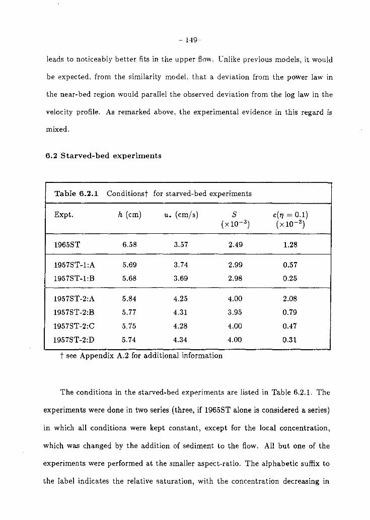
6.2 Starved-bed experiments ............. . 6.2.1 Mean profiles in starved-bed experiments .... . 6.2.2 Discussion: Mean profiles in starved-bed experiments
46 50 52
54
54 54 56 57
69
69 73 76 76 77
81
81 83 85
87
87
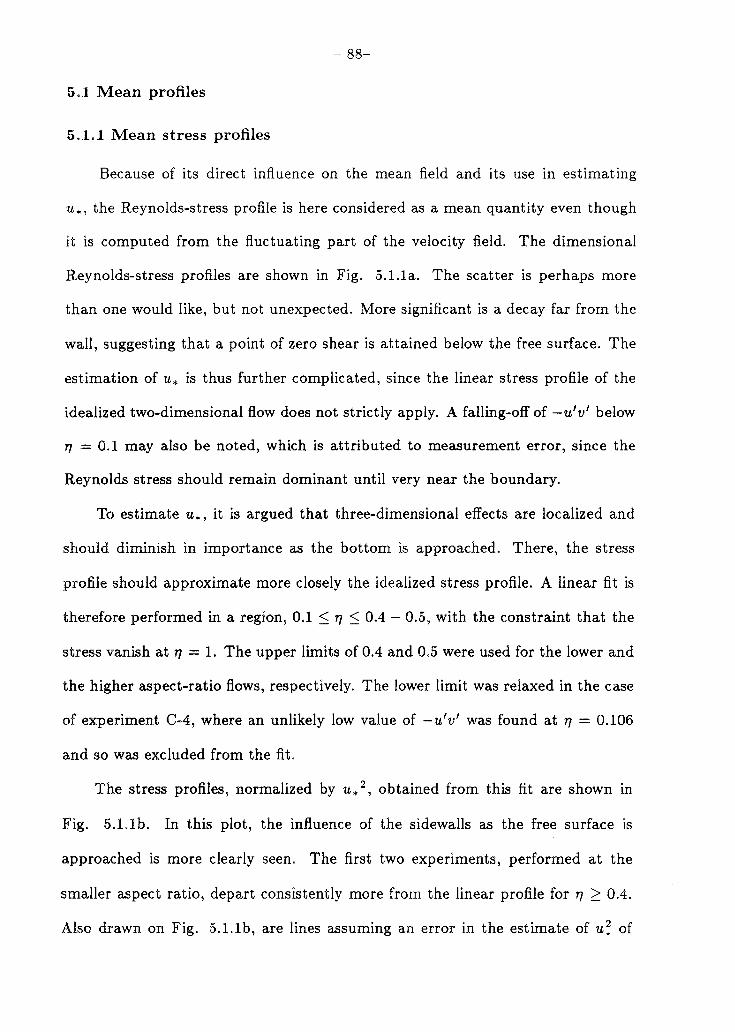
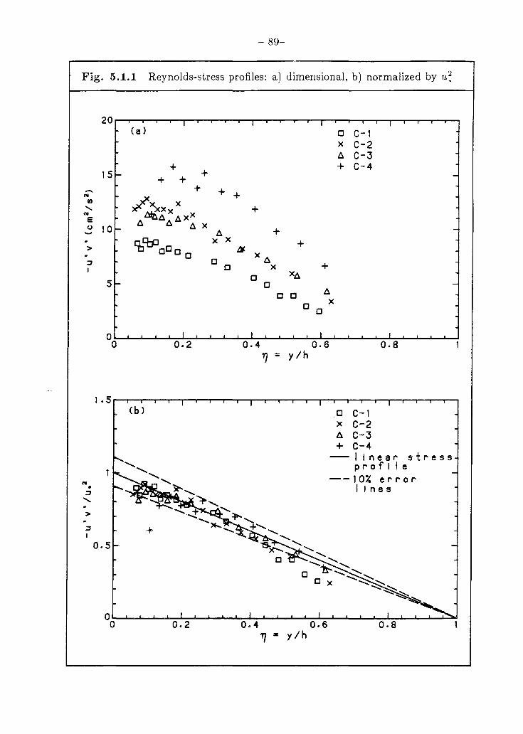
88
88 90
.100
.100
.100 · 101
116 · 116
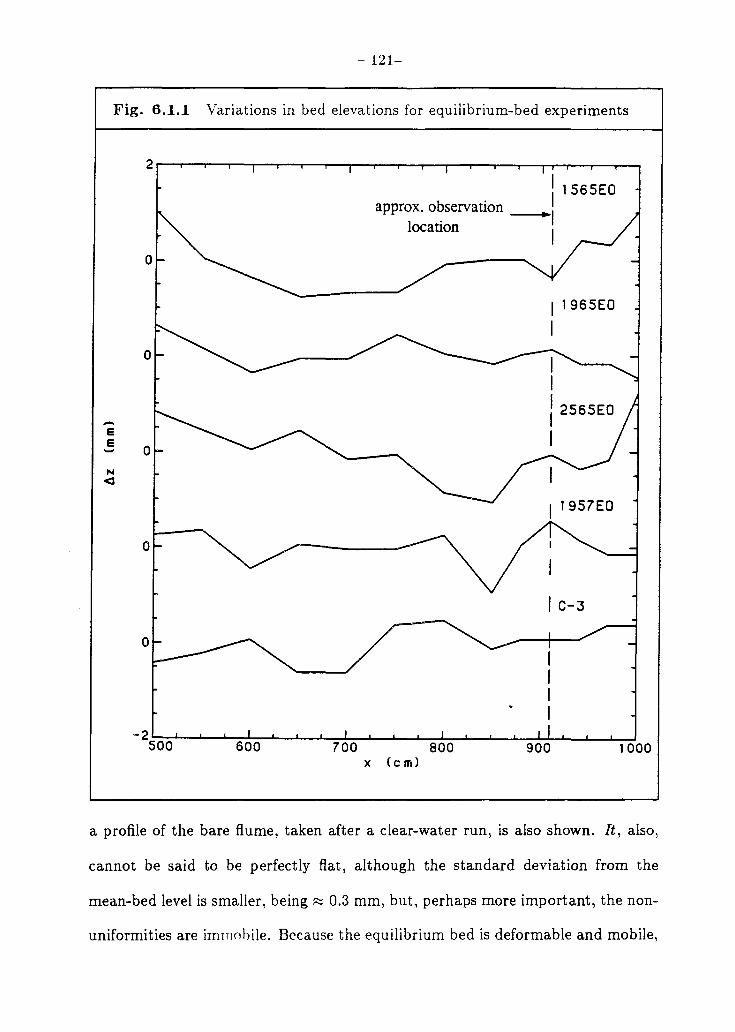
121
· 120
· 120
· 122 · 125 · 133 · 137 .146
· 149 150
· 157
Page 8
- Vll-
6.3 A more specific model ..... < • • • • • • •
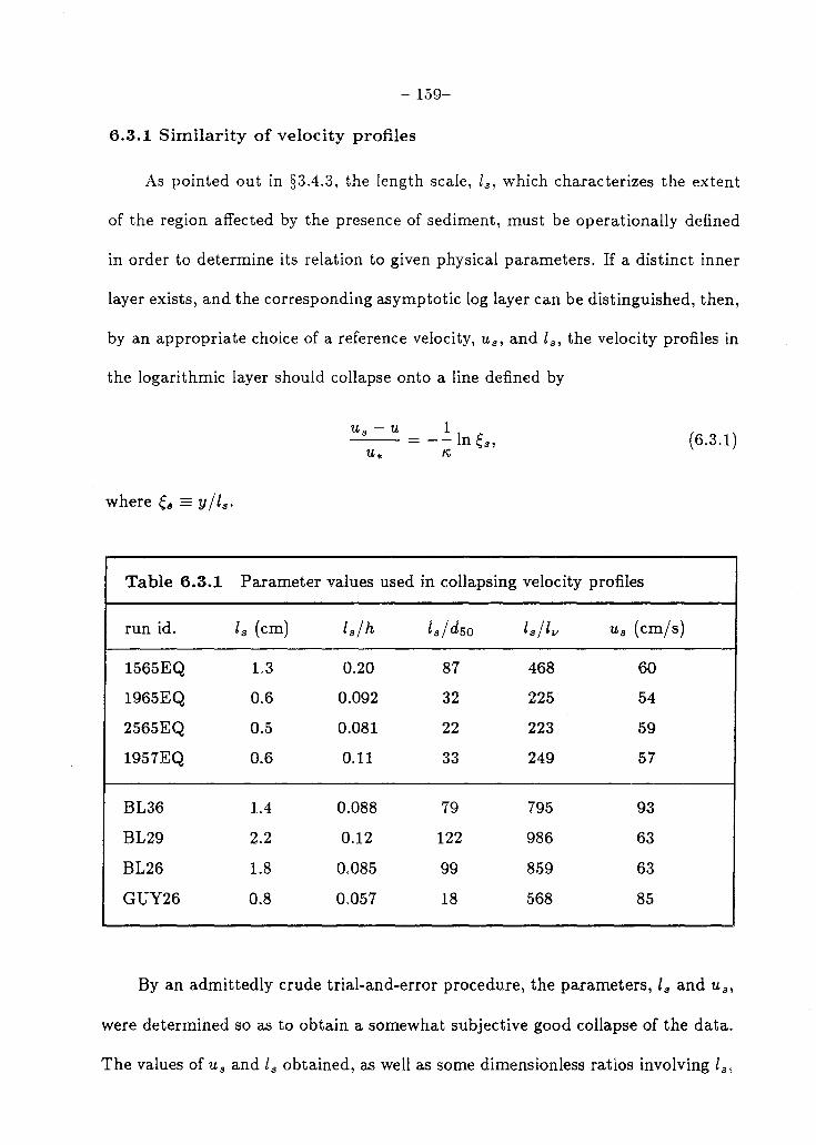
6.3.1 Similarity of velocity profiles . . . . . . . . . 6.3.2 A generalized similarity of concentration profiles
6.4 Results on flow resistance . . . . 6.4.1 Comparison of friction factors 6.4.2 Friction and the velocity profile 6.4.3 Discussion: flow resistance in sediment-laden flows
6.5 Summary
7. Turbulence characteristics
7.0 Introduction . . . . .
7.1 Second-order one-point statistics 7.1.1 Turbulence intensities . . . 7.1.2 Power spectra of velocity fluctuations 7.1.3 Discussion: Second-order one-point statistics
7.2 Higher-order u- and v- statistics
7.3 Results on Reynolds stress statistics
7.4 Summary
8. Summary
8.1 Experimental results . . . . 8.2 Interpretations of experimental results
8.2.1 The traditional model . . . . . 8.2.2 Models based on a stratified-flow analogy 8.2.3 The proposed similarity model
8.3 Open questions ....... .
References
Appendices
A.1 Quadrant analysis A.2 Gross flow characteristics
158 159 166
· 172 · 172 · 175
178
· 179
181
· 181
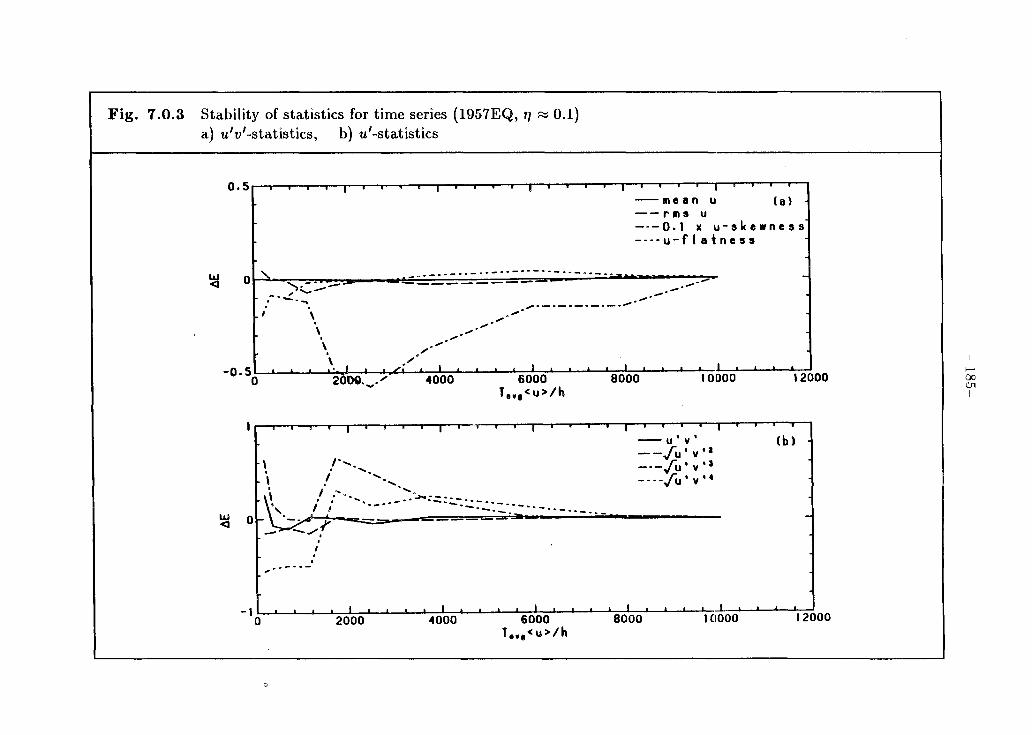
· 186 · 186 · 194 .200
.208
· 218
.226
227
.227
.228
.228
.229
.229
.232
233
.238
.242
Page 10
- viii-
Abstract
Some aspects of turbulence in sediment-laden open-channel flows are exam
ined. A conceptual model based on similarity hypotheses rather than the tradi
tional mixing-length closures is proposed. It is argued that, over a wide range
of laboratory conditions, the main effect of the suspended sediment on the flow
is confined to a layer near the bed. If such a distinct layer can be discerned,
then this is separated from the outer flow by an inertial subregion in which the
mean-velocity profile is approximately logarithmic, with an associated von Karman
constant of ~ 0.4, i.e., the same value as in single-phase flows. It is further shown
that power-law profiles may be derived from general similarity arguments and
asymptotic matching. These implications contrast with those of previous models
in which changes in the mean-velocity profile are supposed to occur throughout
the flow or primarily in the flow far from the bed. Length and concentration scales
appropriate to sediment-laden flows are suggested.
An experimental study was also undertaken. Both the saturated case, in
which a sand bed was present, and the unsaturated case, in which a sand bed
was absent, were investigated. The study was restricted to nominally flat beds,
composed of three well sorted sands (median grain diameters ranged from 0.15
mm to 0.24 rnm). A two-component laser-Doppler-velocimetry system was used
for velocity measurements. Suction sampling was used to measure local mean
concentrations. The major points of the conceptual model are supported by the
experimental results. Higher-order statistics of the velocity field were found to
exhibit little evidence of any effect on the outer flow, supporting the view that
the effect of the suspended sediment is felt primarily in the inner region. This
contrasts with the predictions of recent models that propose an analogy between
sediment-laden flows and weakly stable density-stratified flows.
Page 12
Table
4.1.1
4.2.1
4.2.2
5.0.1
5.1.1
5.1.2
5.2.1
6.1.1
6.1.2
6.1.3
6.2.1
6.3.1
7.1.1
A.2.1
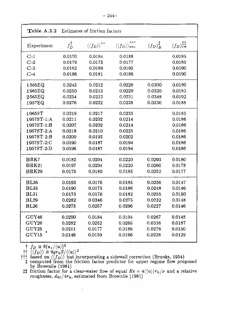
A.2.2
- lX-
List of Tables
LDV system characteristics ............................. .
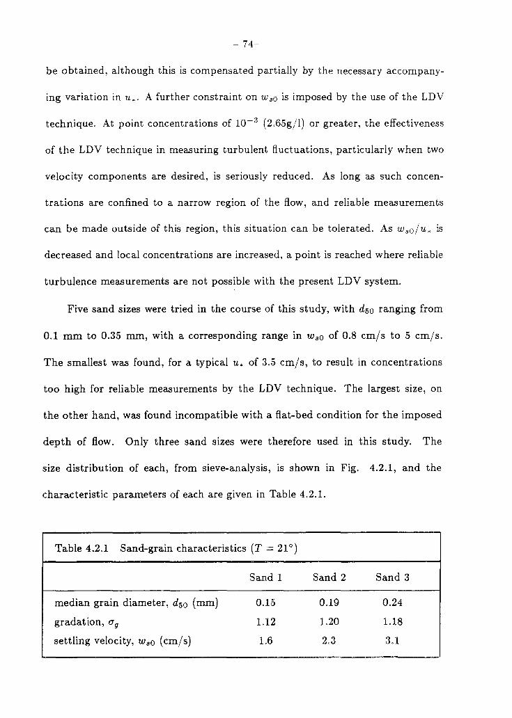
Sand-grain characteristics ............................... .
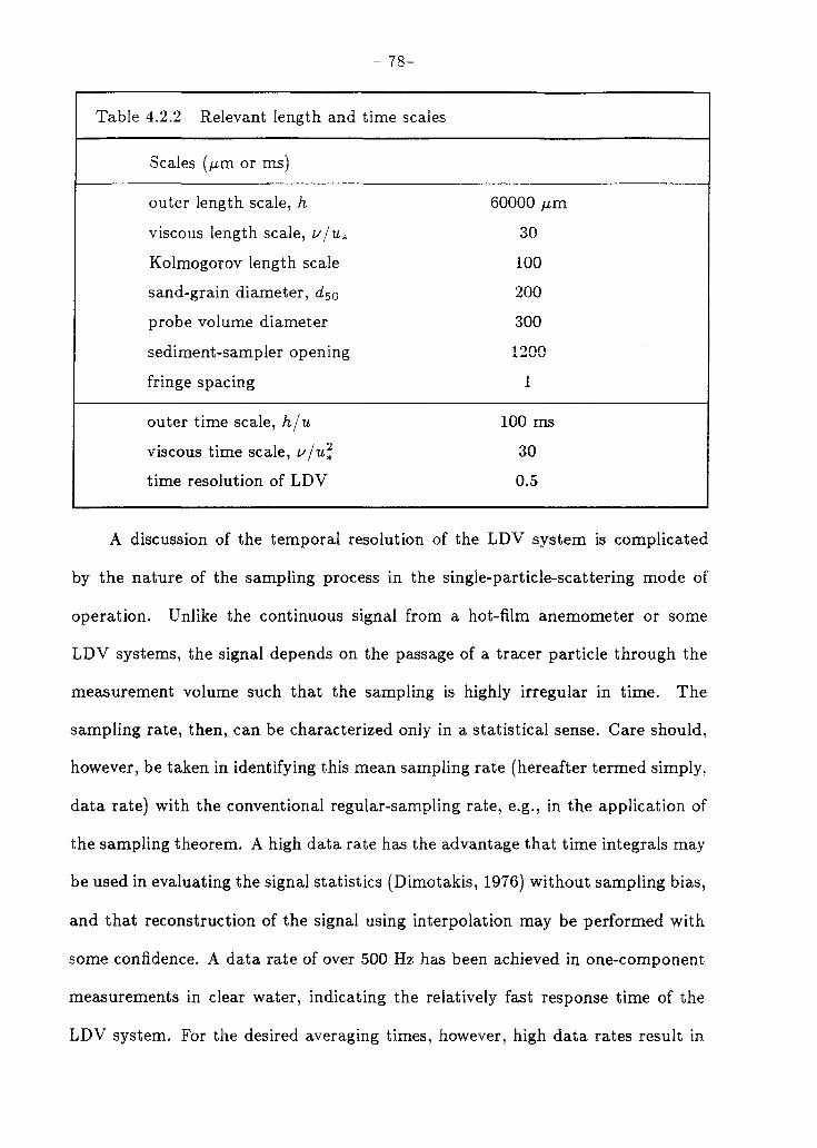
Relevant length and time scales ......................... .
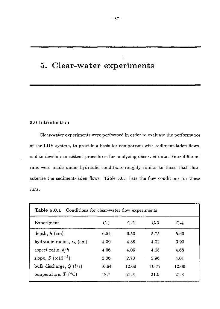
Conditions for clear-water flow experiments ............. .
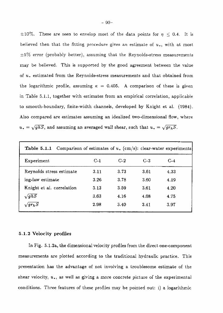
Comparison of estimates of u*: clear-water experiments ..
Computed flow parameters for clear-water experiments
Characteristics of original and interpolated records: clear-water experiments ................................. .
Conditions for equilibrium-bed experiments ............. .
Comparison of estimates of u* (cm/s) ................... .
Conditions for some previous equilibrium-bed experiments
Conditions for starved-bed experiments ................. .
Parameter values used to collapse velocity results ....... .
Characteristics of original and interpolated records ...... .
Summary of flow characteristics: sediment-laden flows ... .
Estimates of friction factors ............................. .
Page
70
74
78
87
90
101
110
122
124
138
149
159
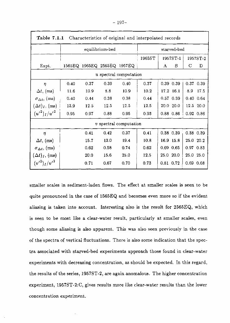
197
243
244
Page 13
- x-
List of figures
Figure Page
2.1.1 Definition sketch ................................................. 7
2.1.2 The Einstein-Chien correlation for Ks (from Vanoni, 1977) ........ 11
4.1.1 Schematic diagram of open-channel flume ........................ 55
4.1.2 Schematic diagram of sediment-sampler .......................... 57
4.1.3 Schematic diagram of LDV system............................... 59
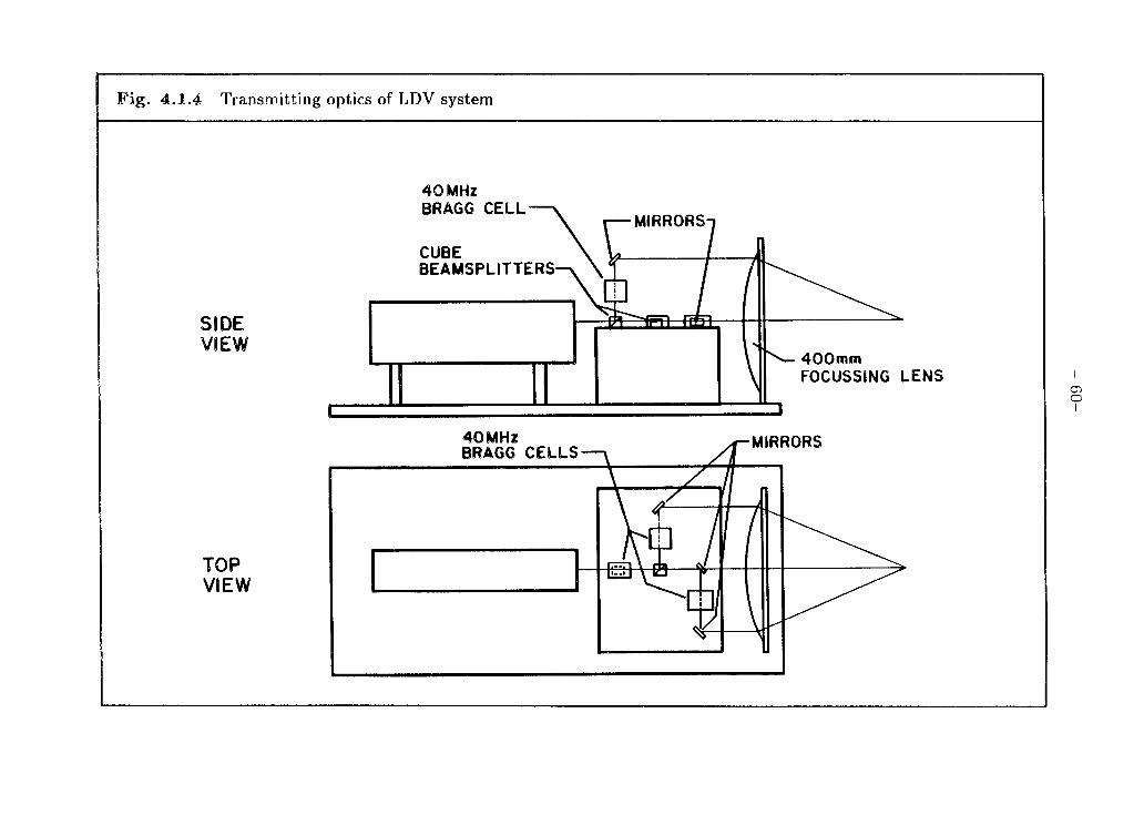
4.1.4 Transmitting optics of LDV system .............................. 60
4.1.5 Configuration of laser beams. ..... . . ..... . .. .. . .. . .. . .. . . . .. . . . . . 62
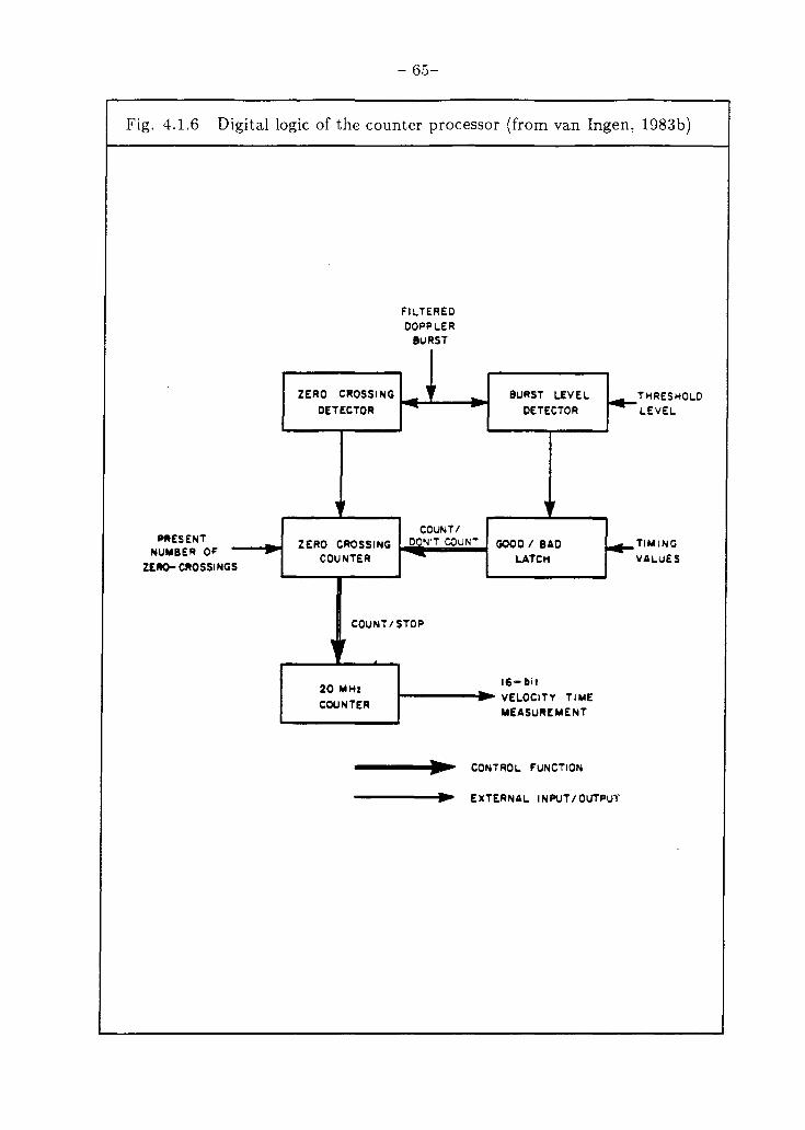
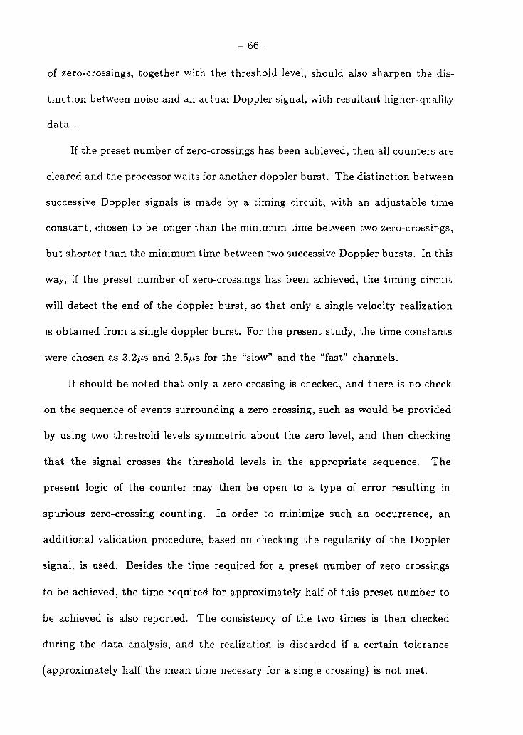
4.1.6 Digital logic of the counter-processor (from van Ingen, 1983b) .... 65
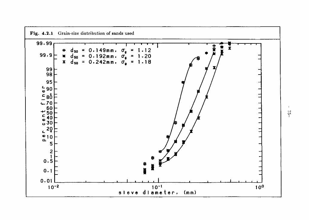
4.2.1 Grain-size distribution of sands used ......... , ... , .......... , . . . . . 75
5.1.1 Reynolds stress profiles: a) dimensional, b) normalized by u;...... 89
5.1.2 a) Dimensional velocity profiles, b) Consistency of I-component, 2-component, pitot-tube results .. 91
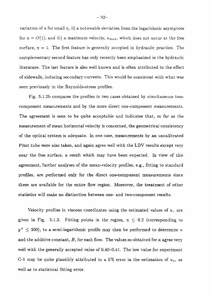
5.1.3 Velocity profiles in viscous coordinates. . . . . . . . . . . . . . . . . . . . . . . . . . . . 93
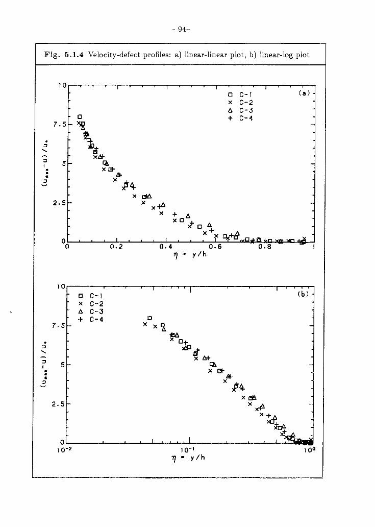
5.1.4 Velocity-defect profiles: a) linear-linear plot, b) linear-log plot.. .. . 94
5.1.5 Velocity-defect profiles, distinguished by aspect ratios: a) b/h = 4.0, b) b/h = 4.7 ........................................ 95
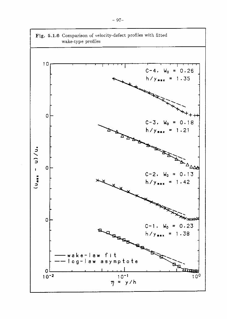
5.1.6 Comparison of velocity-defect profiles with fitted wake-type profiles. . . . . . . . . . . . . . . . . . . . . . . . . . . . . . . . . . . . . . . . . . . . . . . . 97
5.1.7 Mean vertical velocity profiles: a) relative to u, b) relative to u... .. 99
5.2.1 Example of a time series of velocity measurements (from C-2 at TJ = 0.38) ........................................... 102
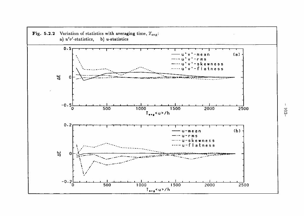
5.2.2 Variation of statistics with averaging time, Tavg
a) u'v'-statistics, b) u- statistics.................................. 103
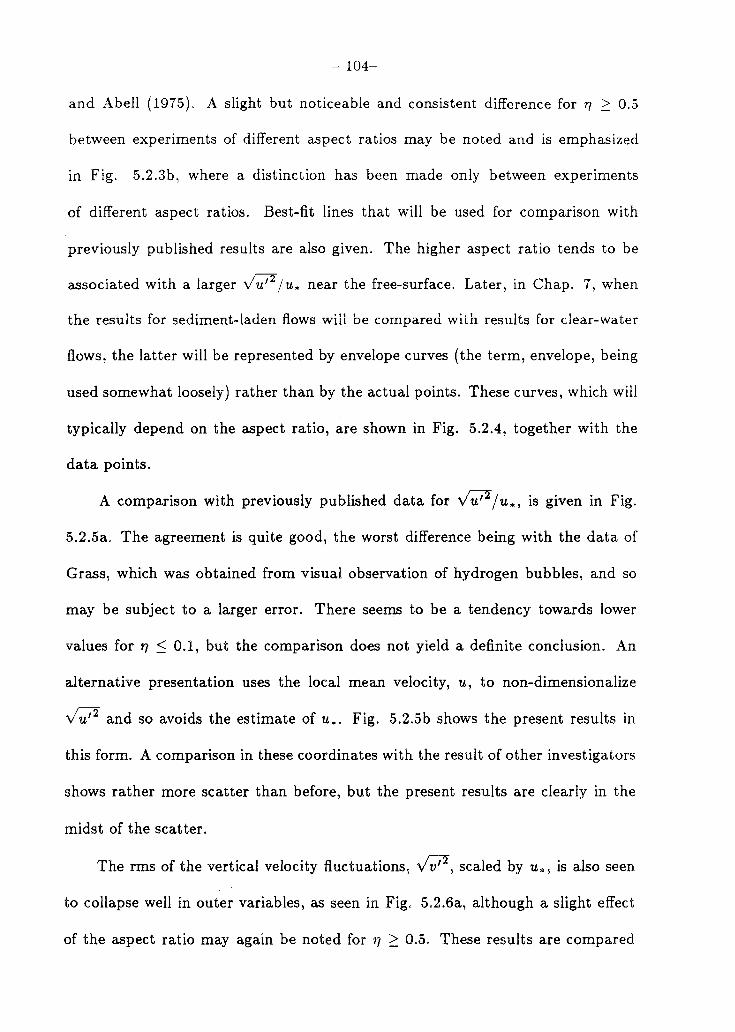
5.2.3 Horizontal turbulence intensities, distinguished by a) experiments, b) aspect ratios. . . . . . . . . . . . . . . . . . . . . . . . . . . . . . . . . .. 105
5.2.4 Envelope of results for horizontal intensities: a) b/h = 4.0, b) b/h = 4.7 ........................................ 106
Page 14
- xi-
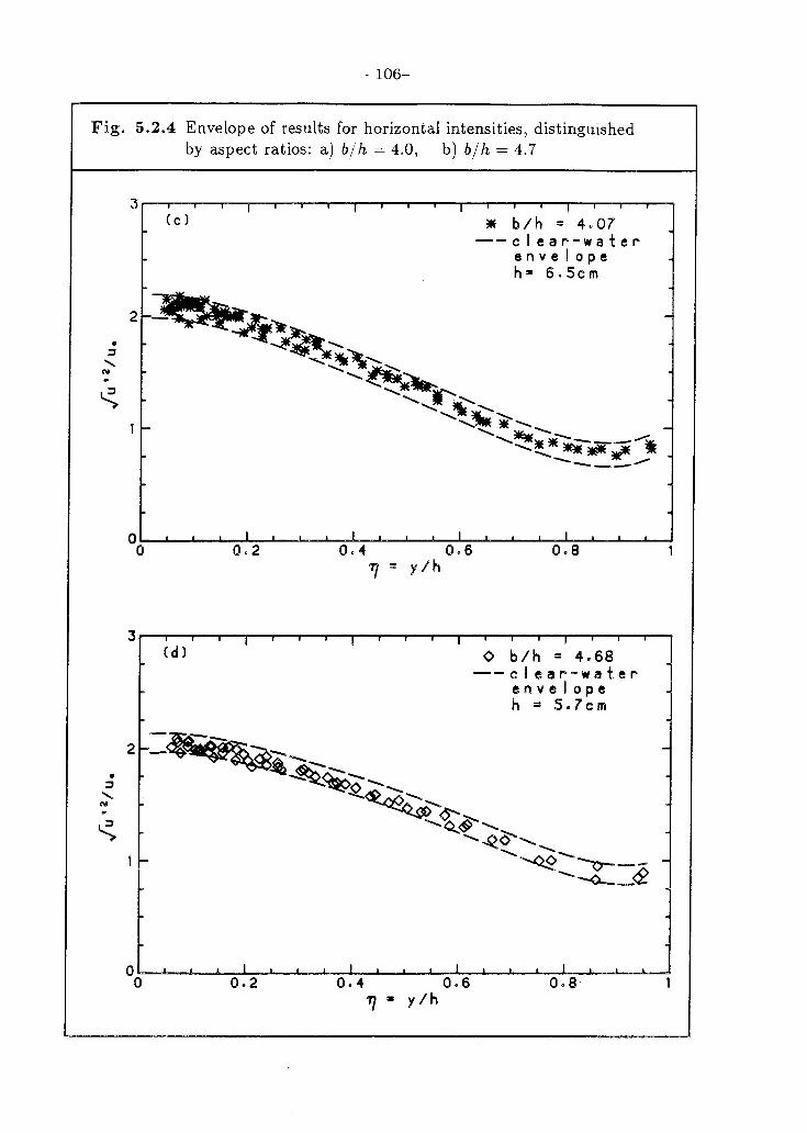
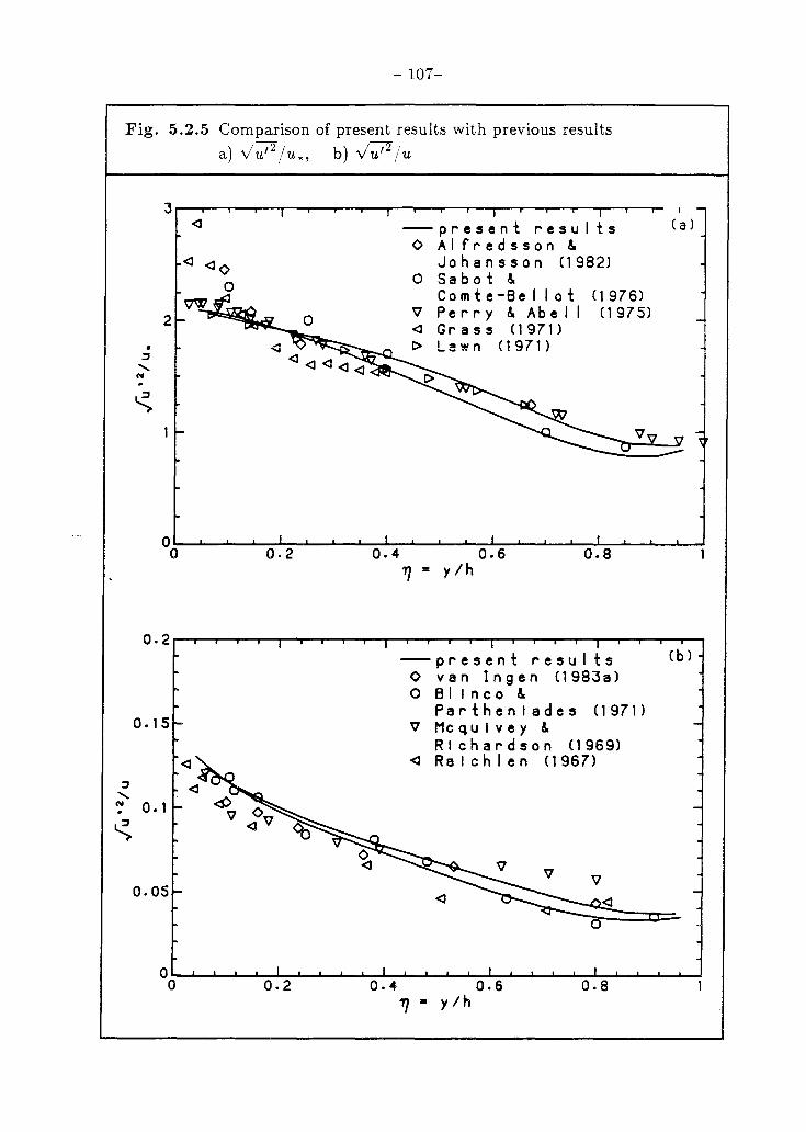
5.2.5 Comparison of present results with previous results
a)v;;J2ju., b)v;;J2ju ............................................ 107
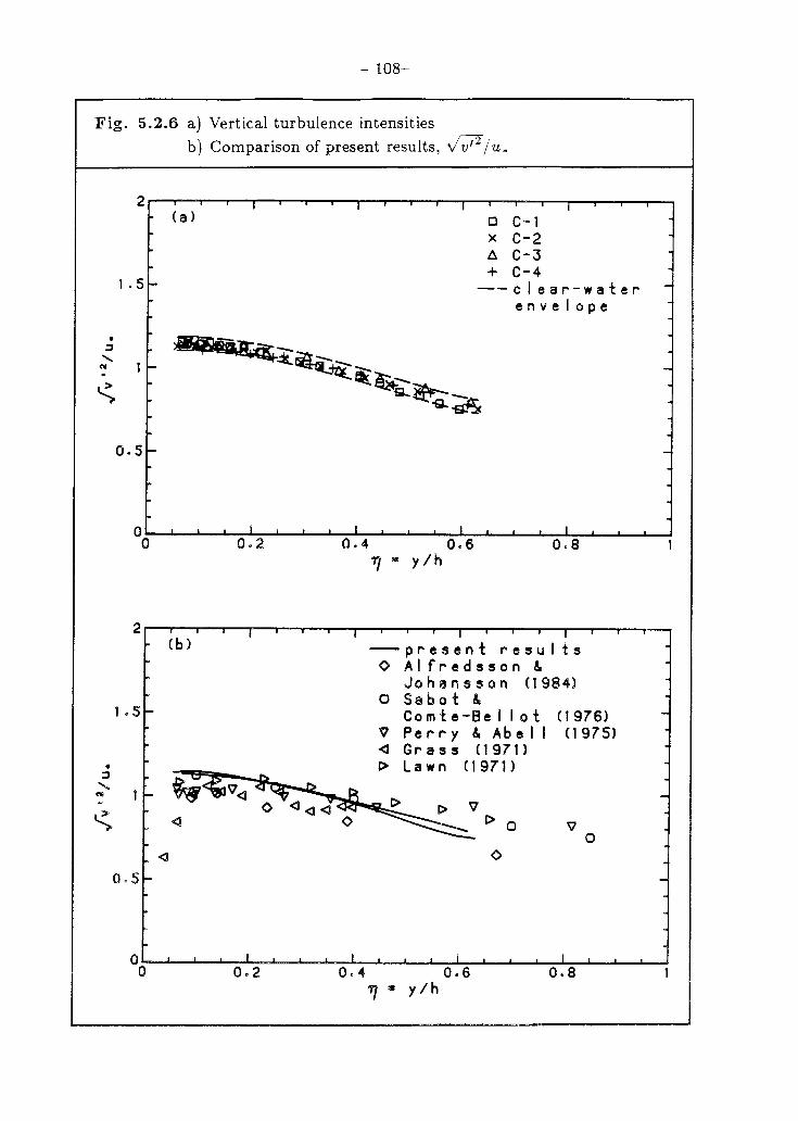
5.2.6 a) Vertical turbulence intensities
b) Comparison with previous results, yf;liju. .................... 108
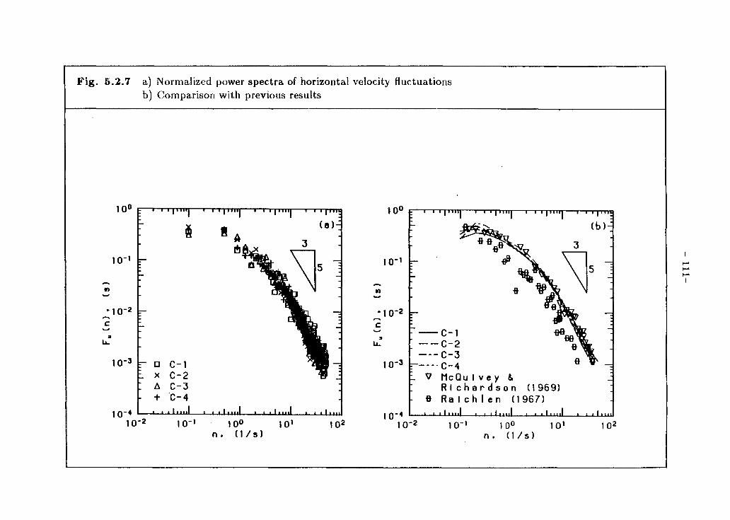
5.2.7 a) Normalized power spectra of horizontal velocity fluctuations b) Comparison with previous results.............................. 111
5.2.8 a) Normalized power spectra of vertical velocity fluctuations b) Comparison with previous results. . . . . . . . . . . . . . . . . . . . . . . . . . . . .. 113
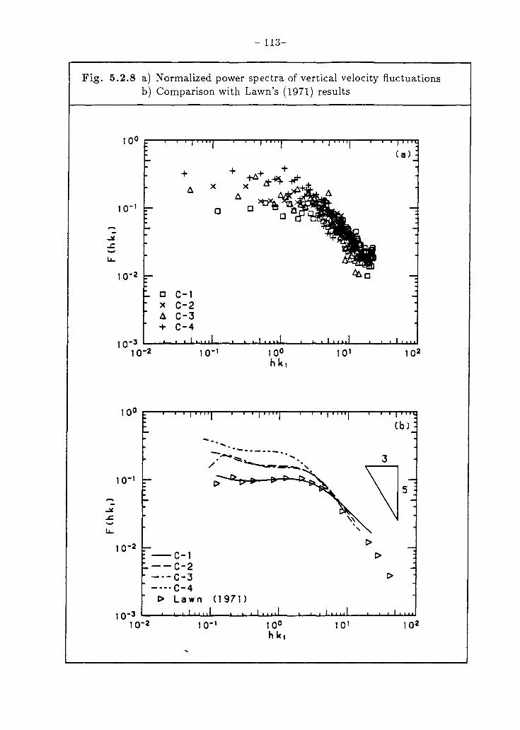
5.2.9 Skewness of a) horizontal, b) vertical velocity fluctuations ........ 114
5.2.10 Flatness of a) horizontal, b) vertical velocity fluctuations ......... 115
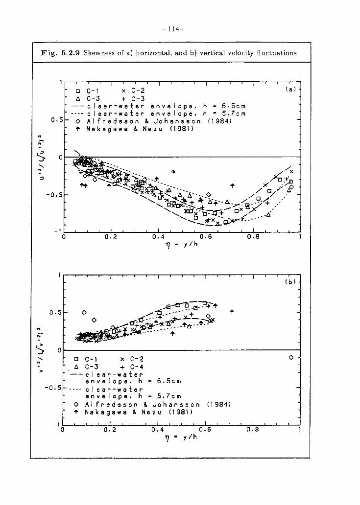
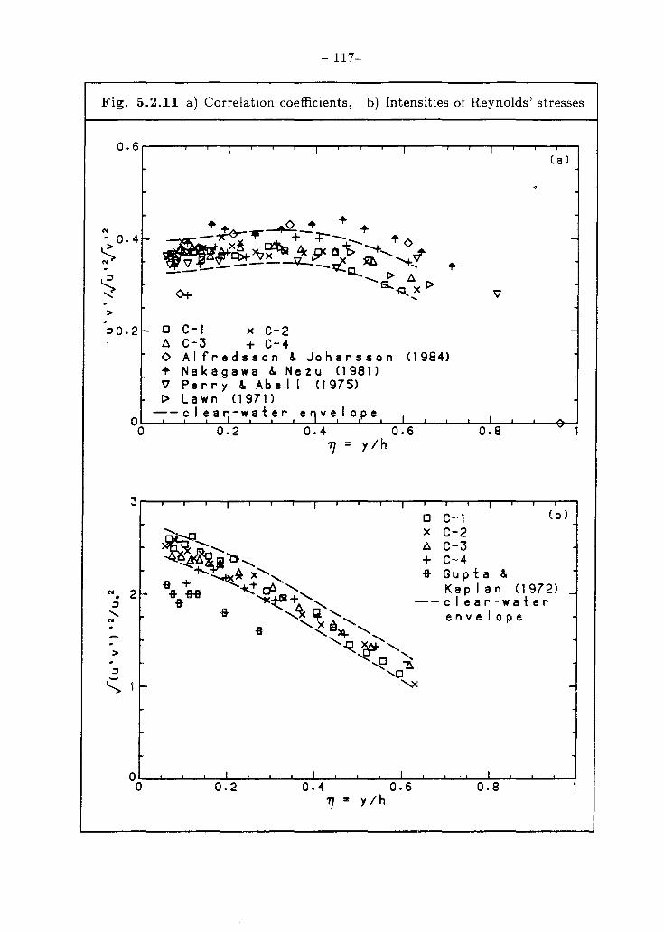
5.2.11 a) Correlation coefficients, b) Intensities of Reynolds stresses ..... , 117
5.2.12 a) Skewness and b) flatness of Reynolds stresses........ ..... .. . .. 118
6.1.1 Variations in bed elevations for equilibrium-bed experiments. . . . .. 121
6.1.2 Reynolds stress profiles: a) dimensional, b) normalized by u: 123
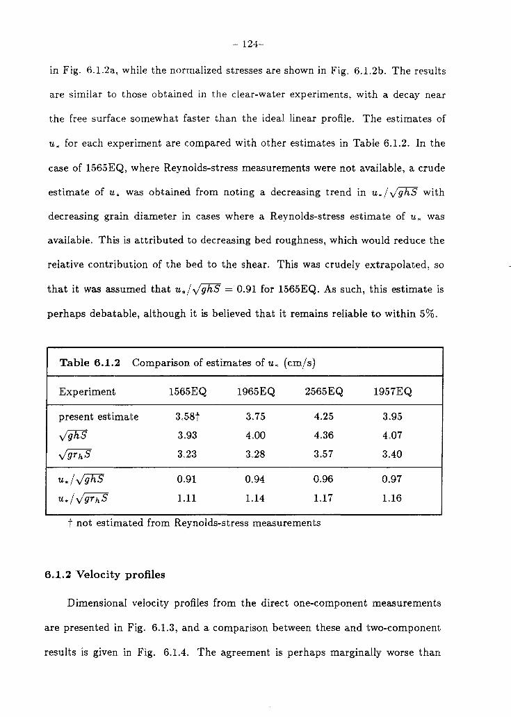
6.1.3 Dimensional velocity profiles a) 1957EQ, 2565EQ, b) 1565EQ, 1965EQ ........................ 152
6.1.4 Comparison of velocity profiles obtained by I-component and 2-component measurements.................................. 126
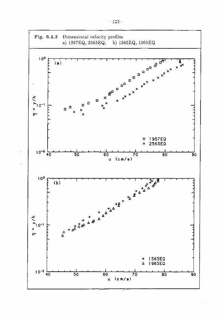
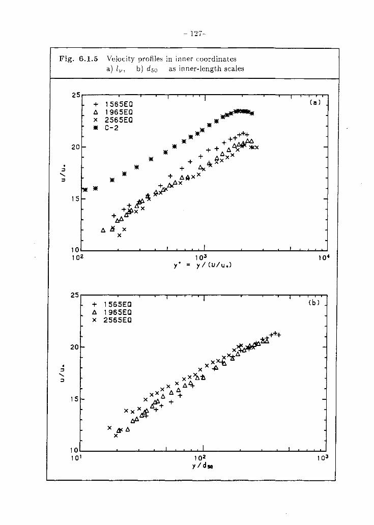
6.1.5 Velocity profiles in inner coordinates a) lv, b) dso as inner length scales................................ 127
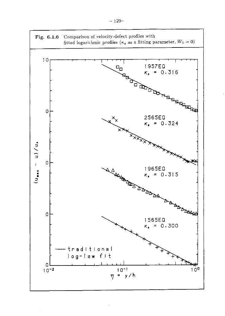
6.1.6 Comparison of velocity-defect profiles with fitted logarithmic profiles (1<;8 as a fitting parameter, Wo = 0) ..... 129
6.1.7 Comparison of velocity-defect profiles with fitted wake-type profiles (Wo as fitting parameter j 1<;8 = 1<;) •••••••• 130
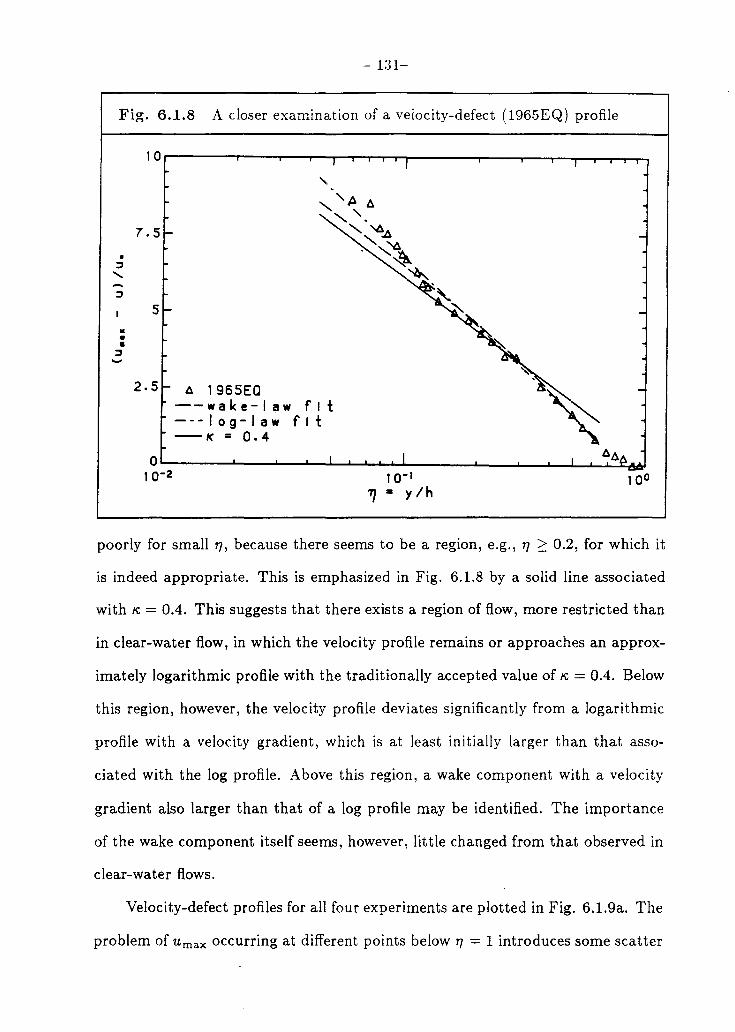
6.1.8 A closer examination of a velocity-defect (1965EQ) profile......... 131
6.1.9 Velocity-defect profiles a) all experiments, b) only 1565EQ and 1965EQ .................. 132
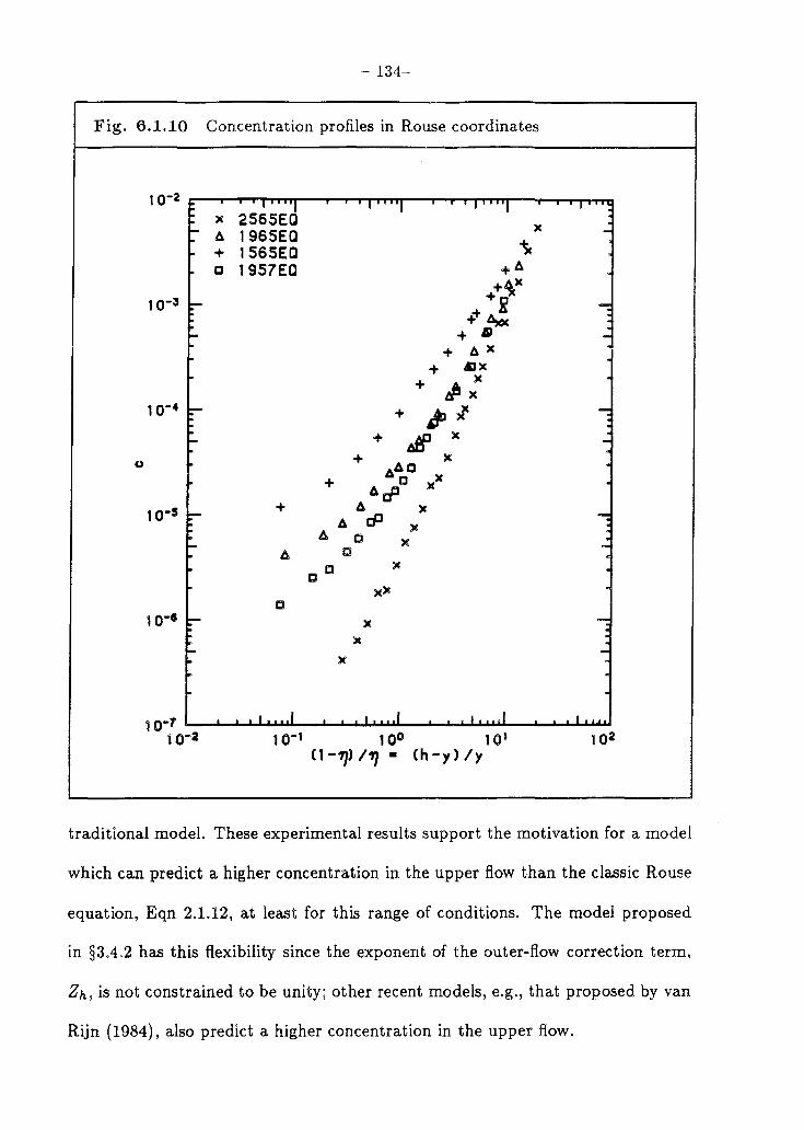
6.1.10 Concentration profiles in Rouse coordinates... .. . . . . . . . . . . ... . . . .. 134
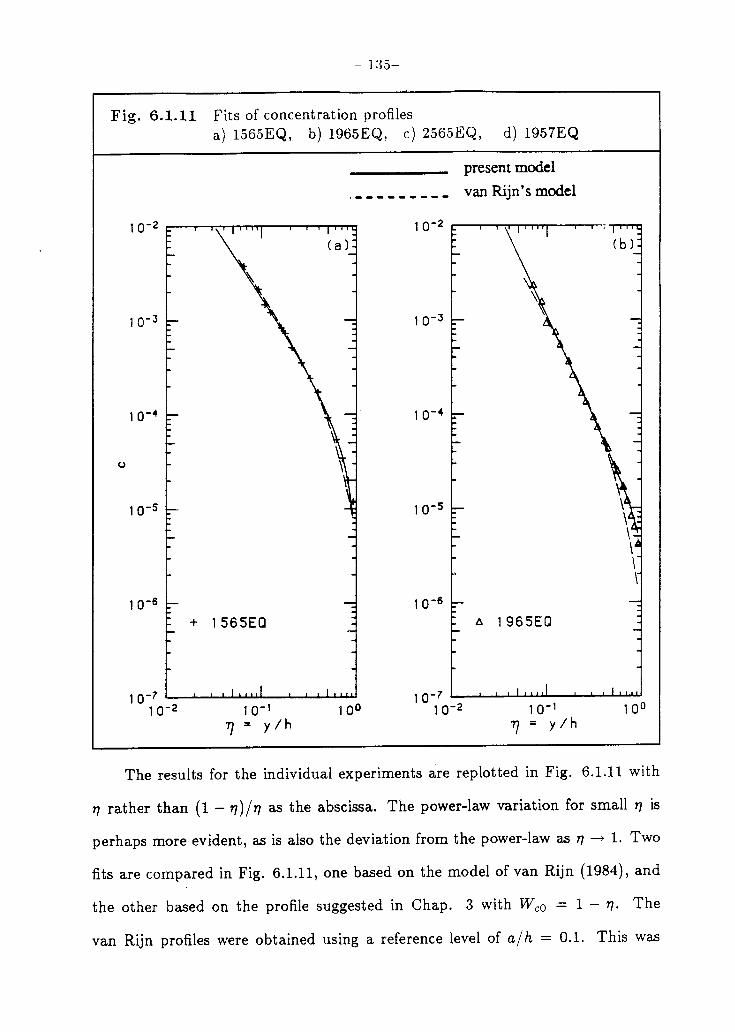
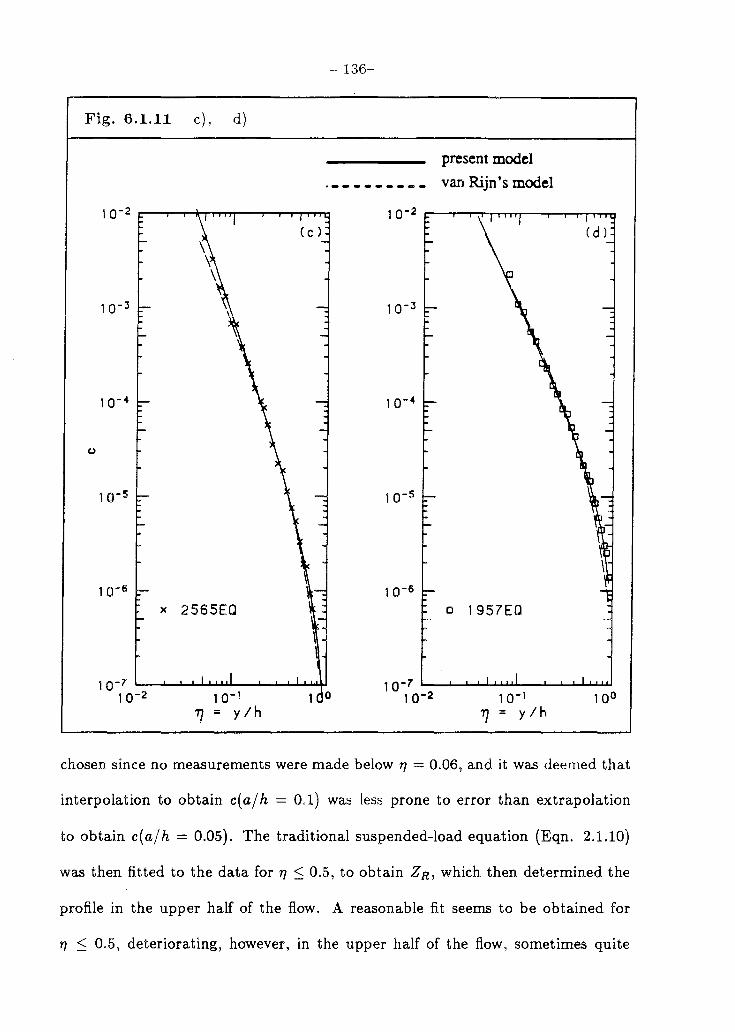
6.1.11 Fits of concentration profiles a) 1565EQ, b) 1965EQ, ..................................... '"'" 135 c) 2565EQ, d) 1957EQ ....................... '" .. .. . .. .. .. .. .. ... 136
6.1.12 Results of Brooks (1954) ................ " ..... ..... .. ....... ..... 140
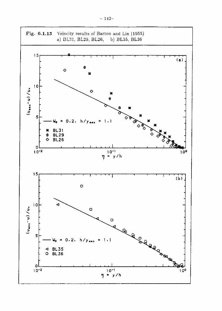
6.1.13 Velocity results of Barton and Lin (1955) a) BL31, BL29, BL26, b) BL35, BL36 ............................ 142
6.1.14 Concentration results of Barton and Lin (1955) a) all experiments examined, b) comparison with traditional fits... 143
6.1.15 Velocity results from Guy et al. (1966) a) GUY26, GUY15, b) GUY46, GUY25 .......................... 145
Page 15
- xii-
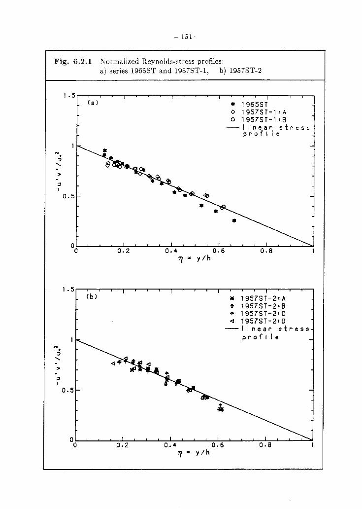
6.2.1 Reynolds stress profiles: a) series 1965ST and 1957ST-1, b) 1957ST-2...................................................... 151
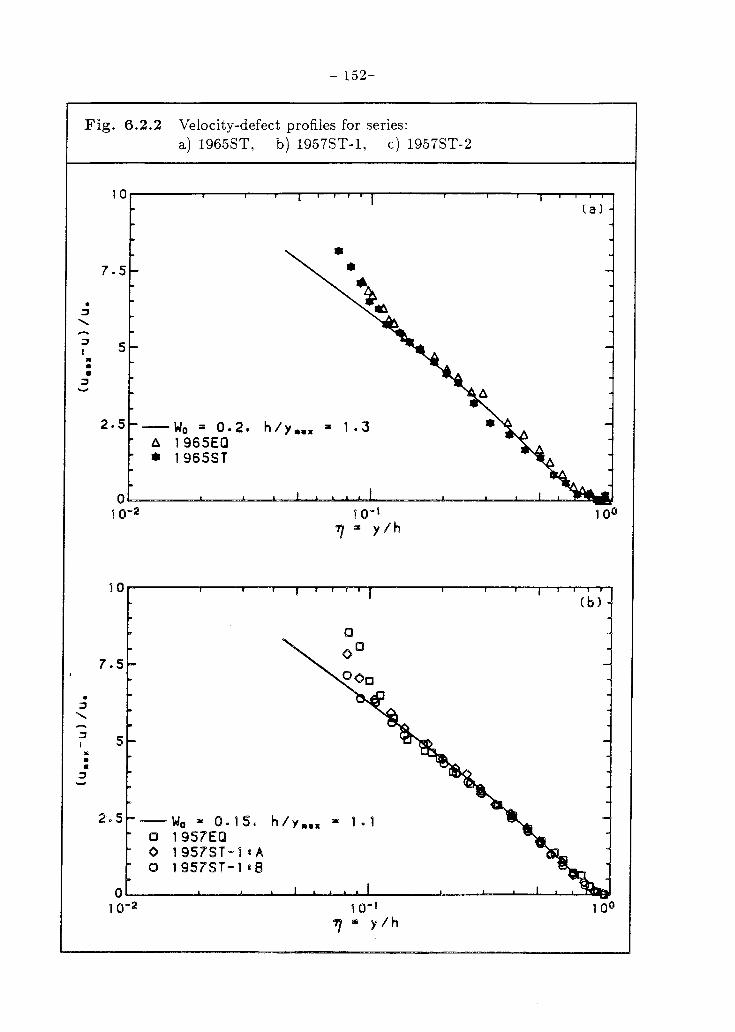
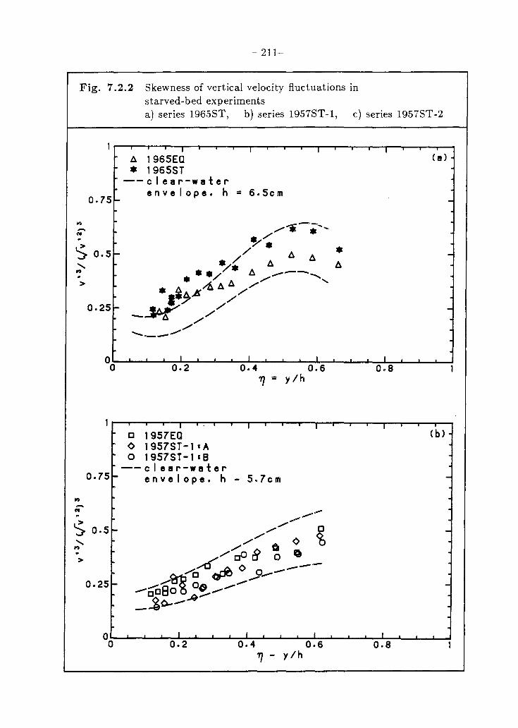
6.2.2 Velocity-defect profiles for series: a) 1965ST, b) 1957ST-1, ......................................... 152 c) 1957ST-2 ..................................................... 153
6.2.3 Concentration profiles for starved-bed experiments ............... 154
6.2.4 Results of Vanoni (1946)........ . . ..... . .. .. . . . .. . . . . . . ... .. . .. ... 156
6.3.1 Velocity profiles of equilibrium-bed experiments, (ls as length scale) a) present results, b) previous results. . . . . . . . . . . . . . . . . . . . . . . . . . . .. 160
6.3.2 Velocity-defect profiles in which no inner layer was discerned ..... 161
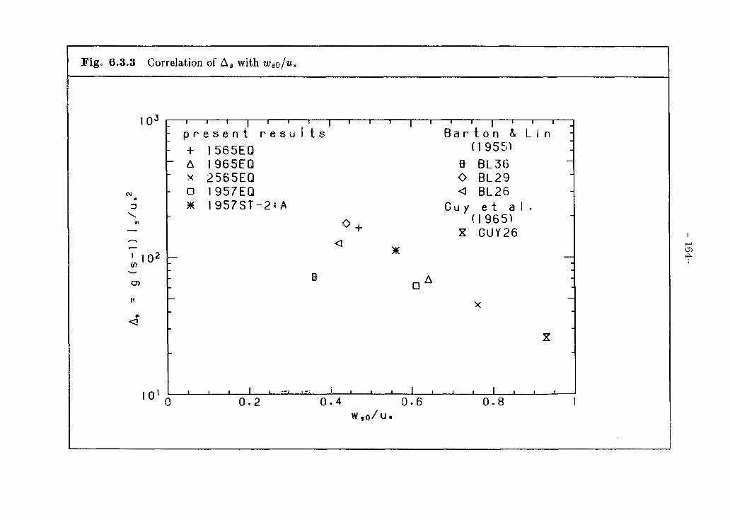
6.3.3 Correlation of ~s with wso/u..................................... 164
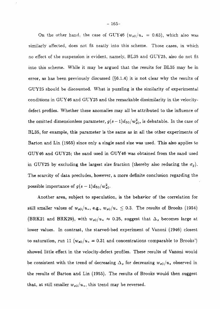
6.3.4 Similarity plot of concentration profiles a) present results, b) results of Barton and Lin (1955) ............ 168
6.3.5 Correlation of C8 with wso/u. .. . .... . . . . .... . .... . .. . ... . .. .... . .. 169
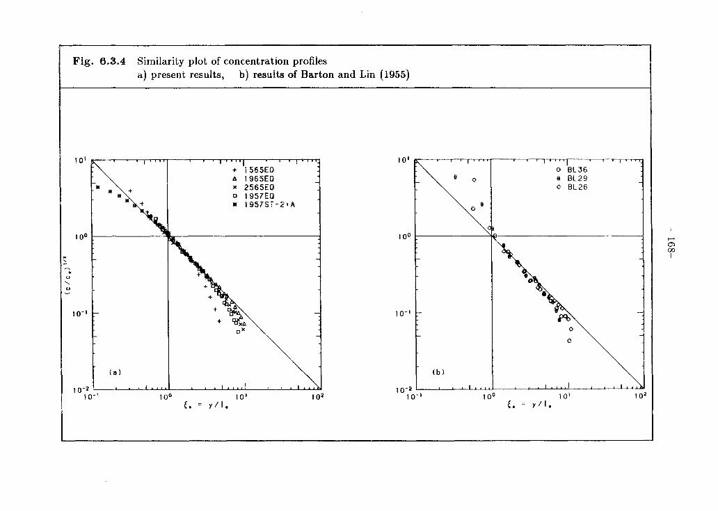
6.3.6 Correlation of Z with wso/u.. . .... . . . ..... . . . .. . ... . . .. . .. . .. .. ... 170
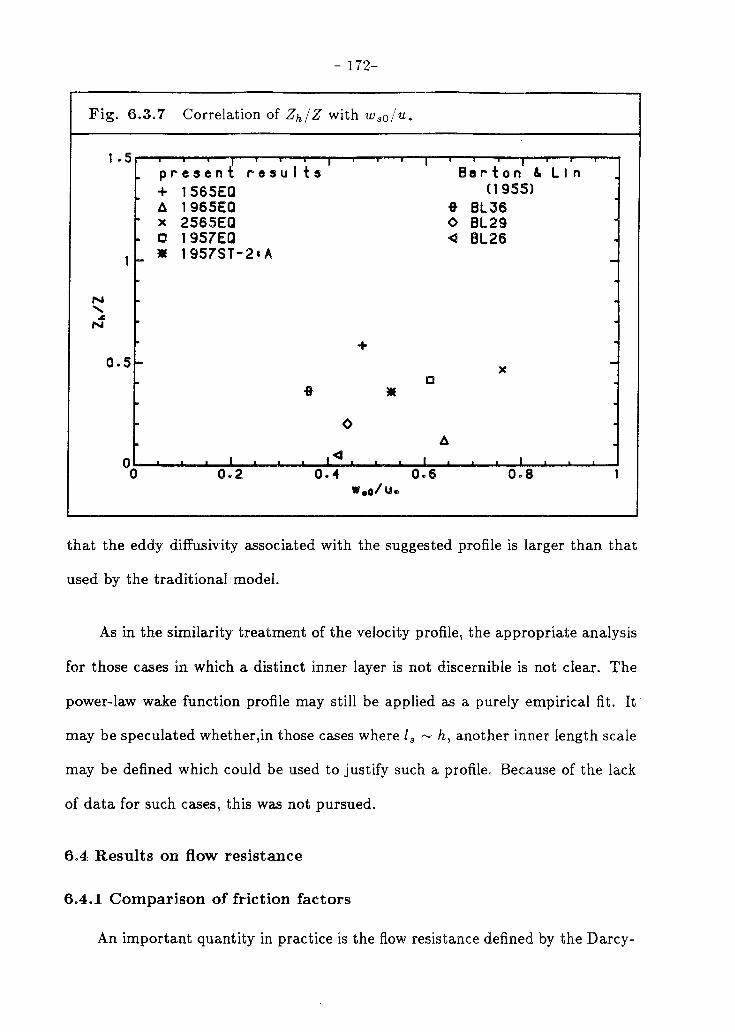
6.3.7 Correlation of Zh/ Z with w 8o/u. ....................... .......... 172
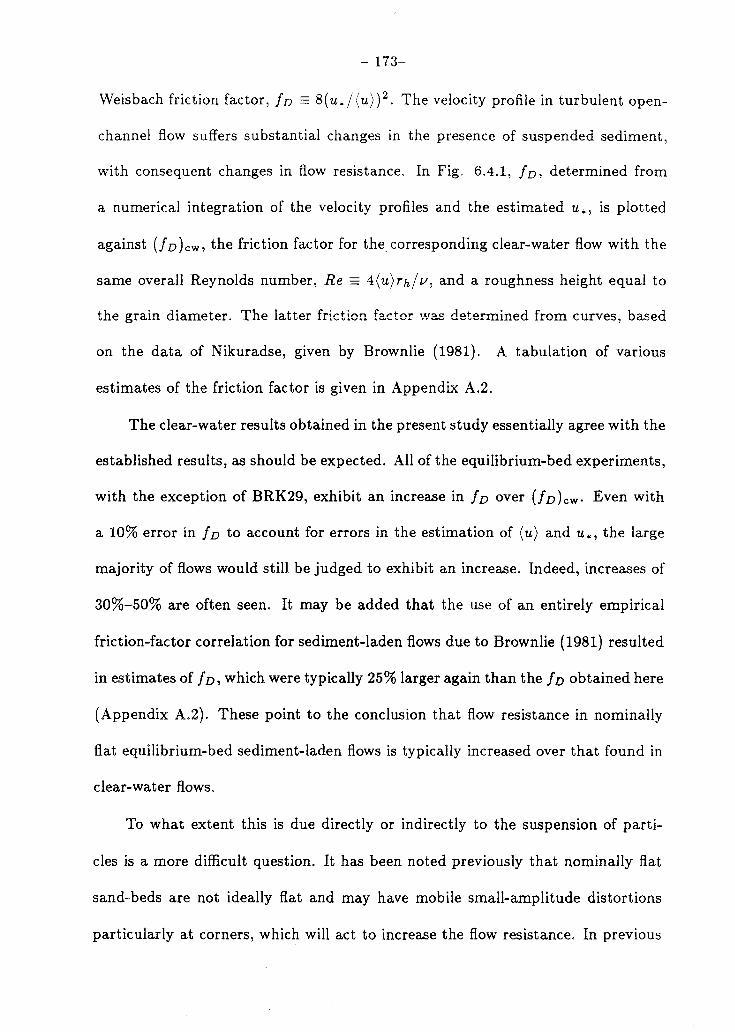
6.4.1 Comparison of flow resistance..................................... 174
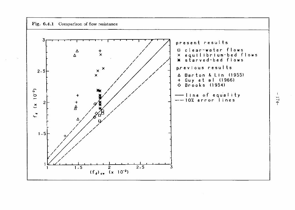
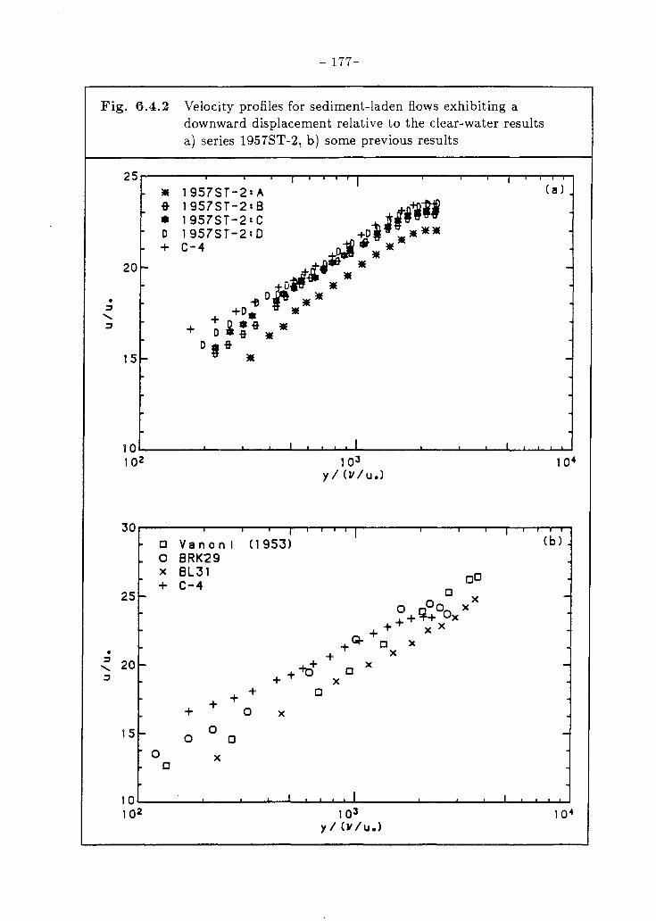
6.4.2
7.0.1
7.0.2
Velocity profiles for sediment-laden flows exhibiting a downward displacement relative to the clear-water results: a) series 1957ST-2, b) some previous results ...................... .
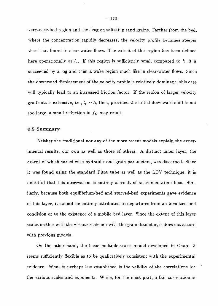
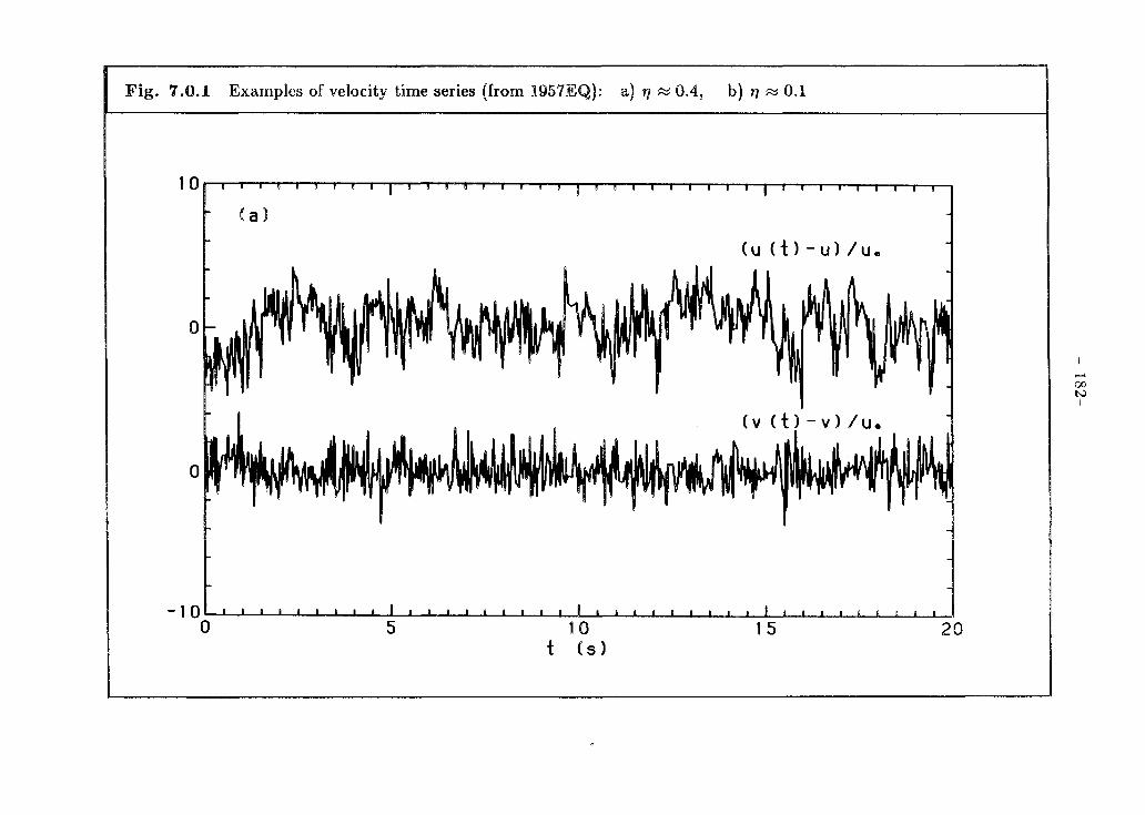
Example of velocity time series (from 1957EQ) a) T'J ~ 0.4, ...................................................... . b)T'J~0.1 ••••••••••••••••••••••••••••••••••••••••••••••• •••••••••
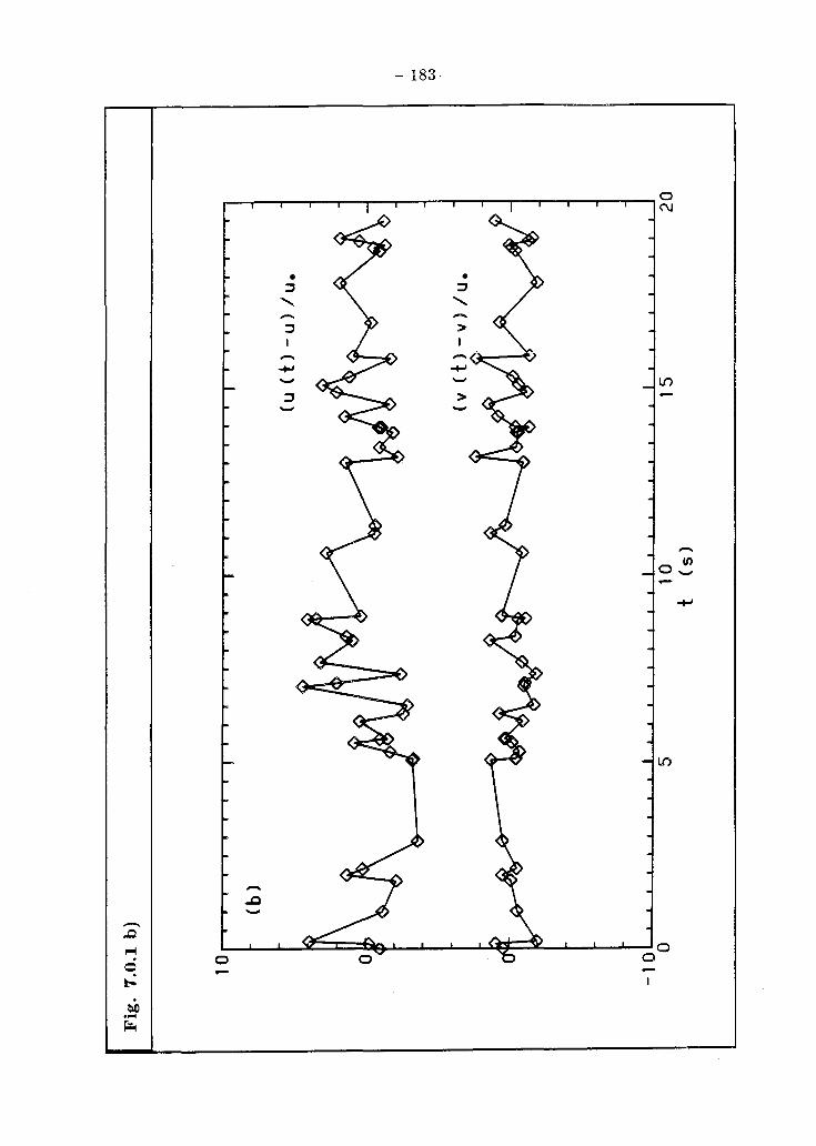
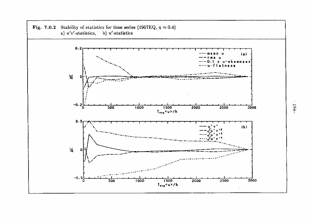
Stability of statistics for time series (1957EQ, T'J ~ 0.4) a) u'v'-statistics, b) u'-statistics ................................. .
177
182 183
184
7.0.3 Stability of statistics for time series (1957EQ, T'J ~ 0.1) a) u'v'-statistics, b) u'-statistics .................................. 185
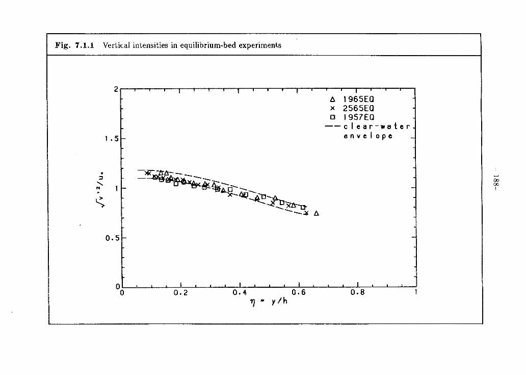
7.1.1 Vertical intensities in equilibrium-bed experiments ............... 188
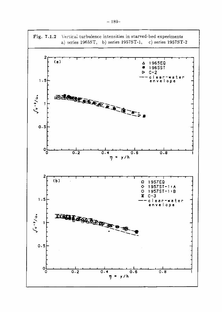
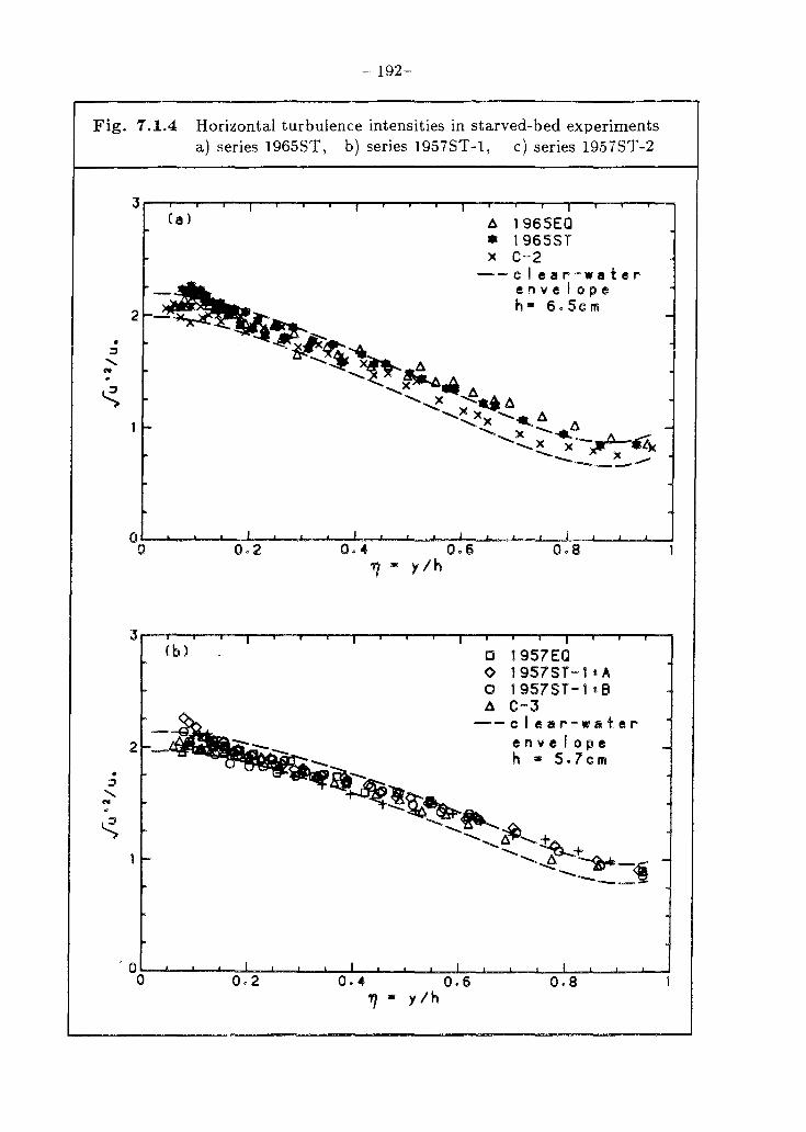
7.1.2 Vertical turbulence intensities in starved-bed experiments a) series 1965ST, b) series 1957ST-1, ............................. 189 c) series 1957ST-2 ............................................... 190
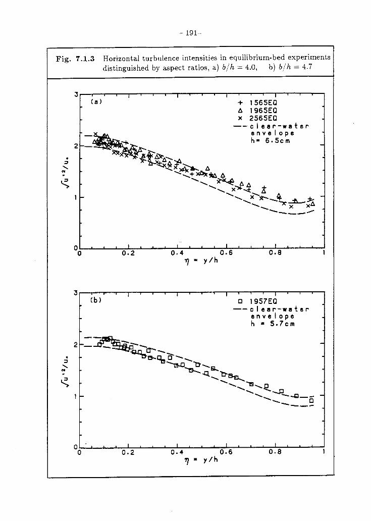
7.1.3 Horizontal turbulence intensities in equilibrium-bed experiments distinguished by aspect ratios, a) b/h = 4.0, b) b/h = 4.7 .......... 191
Page 16
- xiv-
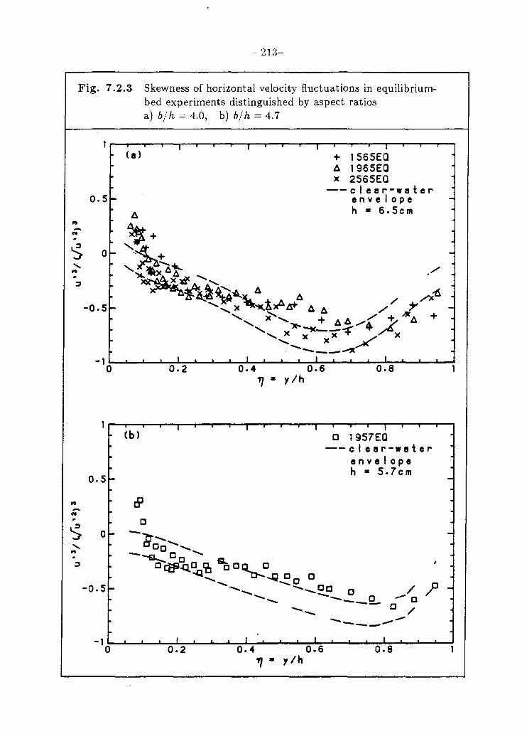
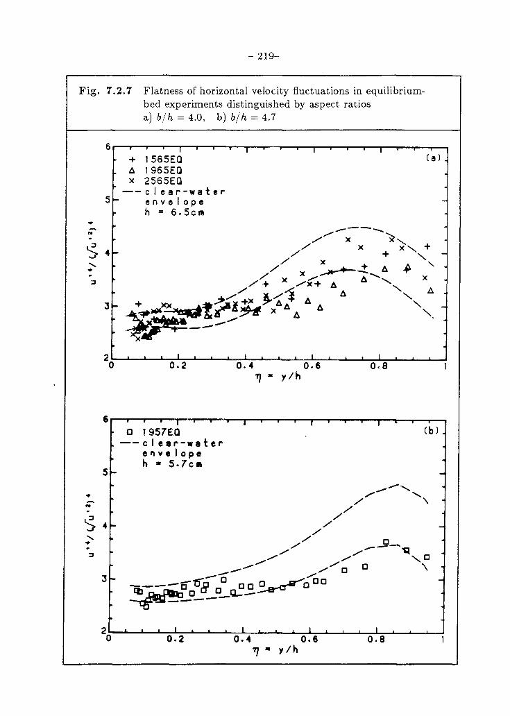
7.2.7 Flatness of horizontal velocity fluctuations in equilibriumbed experiments distinguished by aspect ratios a) b/h = 4.0, b) b/h = 4.7 ........................................ 219
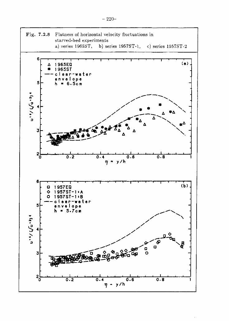
7.2.8 Flatness of horizontal velocity fluctuations in starved-bed experiments a) series 1965ST, b) series 1957ST-l, ............................. 220 c) series 1957ST-2....... ......................................... 221
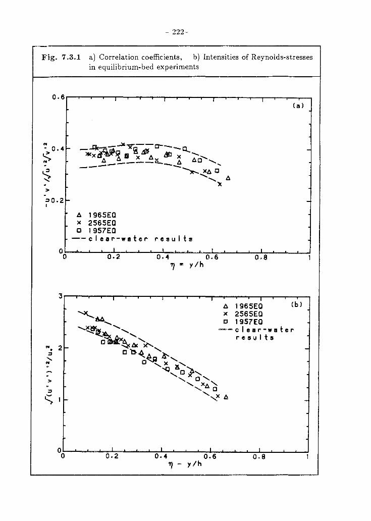
7.3.1 a) Correlation coefficients, b) Intensities of Reynolds stresses in equilibrium-bed experiments. . . . . . . . . . . . . . . . . . . . . . . . . . . . . . . . . .. 222
7.3.2 a) Correlation coefficients, b) Intensities of Reynolds stresses in starved-bed experiments.. . . . . . . . . . . . . . . . . . . . . . . . . . . . . . . . . . . . .. 223
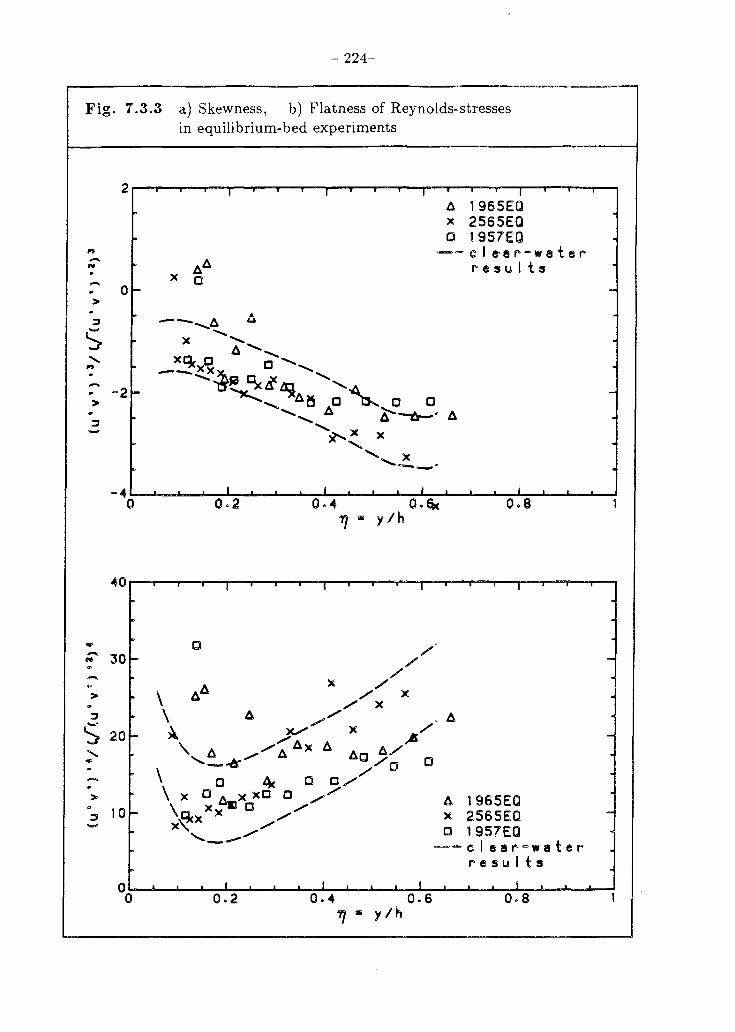
7.3.3 a) Skewness, b) Flatness of Reynolds stresses in equilibrium-bed experiments. . . . . . . . . . . . . . . . . . . . . . . . . . . . . . . . . .. 224
7.3.4 a) Skewness, b) Flatness of Reynolds stresses in starved-bed experiments. . . . . . . . . . . . . . . . . . . . . . . . . . . . . . . . . . . . . .. 225
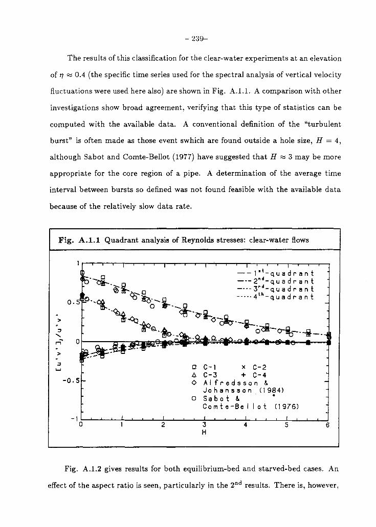
A.I.1 Quadrant analysis of Reynolds stresses: clear-water flows.. . ..... .. 239
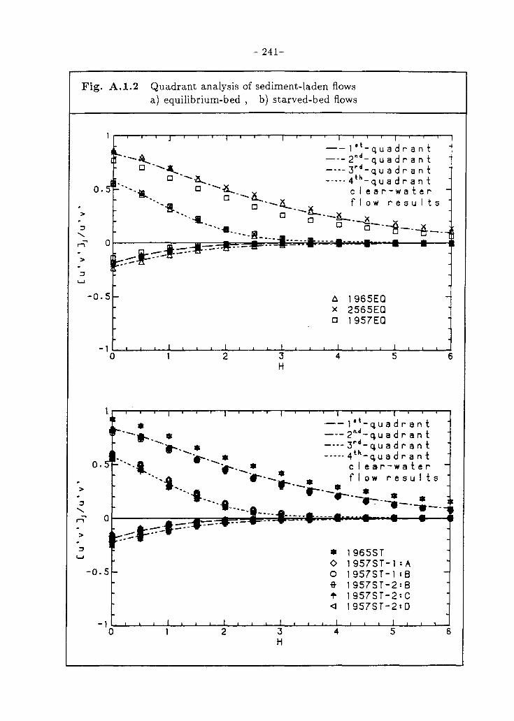
A.I.2 Quadrant analysis of Reynolds stresses: sediment-laden flows a) equilibrium-bed, b) starved-bed flows.......................... 241
Page 17
F
Fr
Fu, Fv
11 , 12 g
h
H
J
k
kl
lK
lm
ls
Lv Lc
Ls
£,
n
P
PI, Ps
Q q ..
r
Th
- XVl-
same as (U D)), but incorporating a sidewall correction (Brooks, 1954)
friction factor for equilibrium-bed upper regime flows predicted from a formula of Brownlie (1981)
friction factor for a corresponding clear-water flow with the same Re = 4(u)rh/v and relative roughness, d5o / 4rh
general outer similarity solution
Froude number, (u) / y'gh
normalized power spectrum of horizontal and vertical velocity fluctuations
general relations between dimensional variables
gravitational constant
depth of flow
hole size, used in quadrant analysis (appendix A.1)
quadrant (1,2,3,or 4) in u' - v' plane
characteristic height of roughness elements
one-dimensional wavenumber related to the frequency, n, by k1 = 21rn/u
general inner length scale
Kolmogorov length scale, (v 3 / c) 1/4
mixing-length
inner length scale specific to sediment-laden flows
viscous length scale, v / tL ..
length scale implicit in bulk Richardson number of Coleman (1981), u:/ g( s - I)eo
Monin-O boukhov length scale defined by Itakura and Kishi (1980), U~/K,W8g(S - 1)(e)
general outer length scale
frequency coordinate of power spectrum
local mean pressure
power parameters used in Einstein-Chien correlation
bulk discharge of flow
constant boundary heat flux in the atmospheric surface layer
general dependent variable
hydraulic radius
Page 18
- XVlll-
V(U'V,),2 root mean square of the Reynolds stress fluctuations
(u'v,),3 /( V(u'v,),2)3 skewness of the Reynolds stress fluctuations
(u'v,),4/( V(u 1v,),2)4 flatness of the Reynolds stress fluctuations
v mean vertical velocity
ii' instantaneous vertical velocity
V;;;Z root mean square of vertical velocity fluctuations
v,3/ (V~/~)3 skewness of the vertical velocity fluctuations
v,4 / (Vv'~)4 flatness of the vertical velocity fluctuations
...(;;;i2 root mean square of the lateral velocity fluctuations
Ws settling velocity of sediment in a turbulent suspension
WsO settling velocity of an isolated particle in a stagnant fluid, defined by a standard drag curve
Wo wake coefficient for the velocity profile
We general wake function for the concentration profile
WeO restricted wake function for the concentration profile
x streamwise coordinate
Y vertical coordinate
Ymax point at which the maximum mean velocity, umqx ,
occurs
vertical coordinate scaled by the viscous length scale, y/lv
deviations from the mean bed elevation
exponent in the concentration power-law
Rouse exponent in suspended-load profile
exponent in the wake-component of the concentration profile
Greek symbols
dimensionless parameter important in both the inner and outer region with respect to the velocity profile
dimensionless parameters important only in either the inner or the outer region with respect to the velocity profile
Page 19
'"Y
Lls
€s
C
<P, <PI, <P2 IC, IC s
.AI, >'2 , .A
l/
17
IT
IT h , ITs
(p)
(};.j
r
e es ;:; ;:; -, -00
- xix-
dimensionless parameters important only in either the inner or the outer region with respect to the concentration profile
dimensionless parameter important in both the inner and the outer region with respect to the concentration profile
reciprocal of the turbulent Schmidt number used in traditional eddy-diffusivity models of vertical turbulent transport
ratio of outer to inner length scales, .c / l non-dimensionalized sediment inner length scale, 9 (s -
1)ls/u;
eddy-diffusivity of vertical sediment transport
rate of dissipation of turbulent kinetic energy
general functions of a single variable von Karman constant in clear-water and in sediment-
laden flows
exponents used in the matching argument
kinematic viscosity
outer coordinate
general function of wso/u.
general dimensionless relation for the outer and inner scales
density of water, the sediment, and the mixture
density of the water-sediment mixture at the bed and at the elevation, Y = Ymax (used by Coleman (1981))
depth-averaged density of the suspension
dummy variable
geometric standard deviation of grain-size distribution
standard deviation of the time interval between velocity realizations
the angles at which the laser beams intersect at the probe volume
mean local shear stress
inner coordinate
inner coordinates specific to sediment-laden flows
general and asymptotic functional form of correlation for ~s
Page 21
- 1-
1. Introduction
Suspended particles are found in large-scale turbulent geophysical flows. In
many cases, these particles are of no dynamic significance and the turbulence may
be studied independently of the presence of particles. In some cases, notably in
flows in natural alluvial channels, the presence of suspended particles may exert
a sufficiently strong influence on the flow so as to invalidate its treatment as a
passive contaminant. The present work is aimed at examining more closely the
interaction between a mostly dilute suspension of sediment with the turbulent flow
that transports it. Although the interest is mainly fundamental, this work may
have implications for solutions to practical problems in the hydraulics of rivers,
reservoirs and estuaries.
Sediment-laden flows pose several problems, A rigorous characterization of
multiphase flows is difficult. Their diluteness has raised questions concerning the
justification of the traditional continuum description. On the other hand, a kinetic
description would seem to present overwhelming difficulties. Compounding the
difficulty of treating two phases is the turbulent nature of the flow. A modest aim
would be a reliable description of the mean field such as has been achieved for
the classic shear flows of a homogeneous fluid, Two coupled fields, the velocity
Page 22
- 2-
and the concentration fields, must be considered. This coupling has traditionally
been underemphasized even though it must be important if it is believed that the
presence of suspended sediment has any significant effect on the turbulent flow.
Although its heterogeneity is due to the presence of two phases, the sediment-
laden flow, with its vertical variation of sediment concentration, has motivated
a recurring analogy to a weakly stable density-stratified flow. Such an analogy
is attractive in its intuitive appeal and offers the possibility of exploiting a large
literature on stably-stratified turbulent flows.
The concept of asymptotic similarity has been central in the development of
useful solutions to problems in turbulent flows but has found little or no system-I
atic application to sediment-laden flows. This may be partly explained by the
historical dominance of mixing-length models, carried over from single-phase flow
problems. Of probably equal importance, however, is that such solutions are most
naturally found in simple flows with a limited number of well-defined length and
velocity scales. Sediment-laden flows are not simple in that appropriate scales are
not known, or are thought to be too many in number to be reduceable to any
simple form. In spite of this, a similarity approach has the advantage of being
rather general because it avoids detailed dynamic considerations. This may be
particularly desirable in the case of a two-phase flow in which even the correct
balance equations may be in dispute.
A number of fundamental questions are prompted by the different aspects of
sediment-laden flows. In view of the uncertainties regarding continuum assump-
tions and the correct equations of motion, can a macroscopic, as against a kinetic,
formulation be developed to describe the mean fields? It will be argued that a
similarity approach may provide a basis for a macroscopic description which does
Page 23
- 3-
not rely on detailed physical models. Also, because it is a turbulent wall-bounded
flow, the question of its similarities to and differences from the more well-known
homogeneous-fluid flows may be raised. Of particular interest in this regard is the
multiple-scales nature that is known to be important for homogeneous-fluid flows.
The possibility of a tractable model offered by the analogy to density-stratified
flows raises the further question: to what extent, if any, is such an analogy valid
for sediment-laden flows? This study will focus on these three questions.
The difficulties posed by sediment-laden flows are not confined to the theo
retical or conceptual plane; experimental problems are many, particularly where
information regarding the fluctuating field is concerned. Traditional probes such
as are used in hot-film-anemometry must be physically delicate in order to satisfy
frequency-response requirements. Sediment-laden flows, however, present a harsh
environment for which a more robust probe is necessary. In this study, the more
recently established laser-Doppler velocimetry (LDV) technique is used. Its opti
cal probe is immune to physical wear, incurs no calibration drift, and is capable
of an adequate frequency response. Problems of interpretation of data due to the
presence of particles other than tracer particles do accompany this use of the LDV
technique. The pragmatic approach taken here has been to interpret the measure
ments, keeping in mind a possible reduced reliability in regions of high sediment
concentration. In such regions, the LDV technique is severely limited in any case
because of the attenuation of both incident and scattered light.
In view of the coupled nature of the problem, it would be desirable exper
imentally to treat the velocity and the concentration fields on an equal footing.
Unfortunately, the availability of more sophisticated velocity-measuring instru
ments results in a disproportionate amount of information on the velocity field
Page 24
- 4-
compared to the concentration field. An additional problem associated with the
concentration field is the ill-defined nature of fluctuating quantities, a consequence
of the uncertainties of the continuum description. This study, in common with pre
vious studies, is limited then to the mean concentration field, which is determined
by the traditional suction-sampling technique.
Although it is hoped that this work has implications for river hydraulics, it
examines a rather idealized flow. Only flows uniform in the streamwise direction,
at least over the working section, are considered. These include both flows in
which a sand bed exists in equilibrium with the suspension, i.e., equilibrium-bed
flows, and flows in which no such sand bed exists, i.e., starved-bed flows. As
interest is on the effect of suspended sediment on turbulence, the equilibrium-bed
experiments are restricted to beds that are nominally flat. Although natural sands
are used in the experiments, the sands are well sorted, and thus highly uniform in
size distribution compared to that typically found in natural channels. The size
range is also above that in which cohesion between particles would be important,
so that effects of cohesion are not considered.
A critical review of the traditional and the more recent approaches to describ
ing the mean fields is given in Chap. 2. A conceptual framework for thinking about
the mean fields in sediment-laden flows is developed in Chap. 3. The ideas of mul
tiple scales, asymptotic matching, and similarity are crucial in this development.
Appropriate length, velocity, and concentration scales are suggested.
A description of the apparatus and instrumentation used in the experimental
part of this work may be found in Chap. 4. Results of sieve analyses of the sand
grains used are also presented. Experimental design is discussed in terms of the
type of experiments performed, the constraints limiting the range of experimental
Page 25
- 5-
conditions obtainable, and the statistical requirements for representative turbu
lence characteristics. The procedure followed in performing experiments is also
outlined.
Experimental results are presented and discussed in Chaps. 5-7. Both the
mean and the fluctuating fields of clear-water flows, i.e., those with no suspended
sediment, are considered first. These results form the basis for comparison with
results in sediment-laden flows. The results for the mean fields in sediment-laden
flows are then considered with interest being centered on the range of validity of the
various proposed models. Finally, the fluctuating velocity field, as characterized
by its statistics, is examined.
Page 26
- 6-
2. Background and literature review
2.1 A review of previous theoretical work
2.1.1 Uniform fully developed open-channel flow without sediment
Consider a steady, turbulent, open-channel, gravity-driven flow of depth, h,
uniform in the mean-flow direction (the x-direction), over a smooth surface of
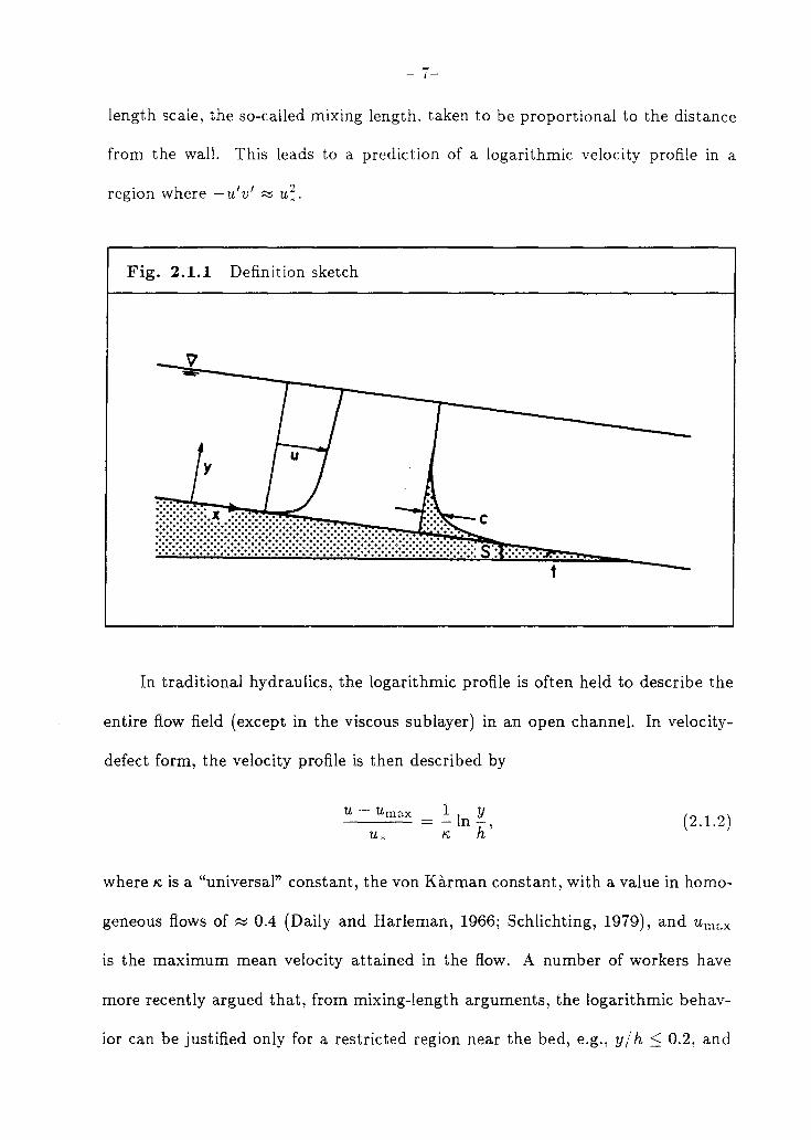
infinite extent, inclined at a slope, S. A definition sketch is given in Fig. 201.1.
The longitudinal momentum equation reduces to
r(y} du -- = -u'v' + 1/- = u:(l - y/h), Pw dy
(201.1)
where r(y) / Pw is the shear stress, -u'v' is the Reynolds stress, 1/ is the kinematic
viscosity, u. is the shear velocity, h is the depth of flow, and Pw is the density
of water. For convenience, time-averaged quantities will not be denoted with an
overbar. In the bulk of the flow, where viscous effects are negligible, the shear
stress is primarily carried by the Reynolds stresses, which should then follow a
linear profile. The classical solution to the closure problem posed by Eqn. 2.1.1 is
the mixing-length hypothesis of Prandtl. This hypothesis relates the fluctuating
velocites, iL' and v', and their correlation, to the mean-velocity gradient and a
Page 27
- 7-
length scale, the so-called mixing length, taken to be proportional to the distance
from the wall. This leads to a prediction of a logarithmic velocity profile in a
region where -u'v' ~ u:.
Fig. 2.1.1 Definition sketch
v -
{~~~~ ~~ ~ ~ ~ ~ ~~ ~ ~ ~~~ ~ ~~~? ~~} ~~ ~ ~ ~~ ~~ ~ ~} ~ ~ ~ ~ ~ ~ ~ ~ ~~ ~~ ~ ~ ~~ ~ ~ ~ ~:~: ~: ~: ~:::~: ~ ~ ~ ;~;:;::::: S·: .:.:.: ..... 1
In traditional hydraulics, the logarithmic profile is often held to describe the
entire flow field (except in the viscous sublayer) in an open channel. In velocity-
defect form, the velocity profile is then described by
U - U max 1 Y = -In
K., h' (2.1.2)
where K., is a "universal" constant, the von Karman constant, with a value in homo-
geneous flows of ~ 0.4 (Daily and Harleman, 1966; Schlichting, 1979), and U max
is the maximum mean velocity attained in the flow. A number of workers have
more recently argued that, from mixing-length arguments; the logarithmic behav-
ior can be justified only for a restricted region near the bed, e.g., y / h :::; 0.2, and
Page 28
- 8-
that, for y / h ~ 0.2, a correction to the logarithmic function is necessary. Cole-
man and Alonso (1983) suggested the use of the wake-function that was originally
proposed by Coles (1956) to describe turbulent boundary-layer flow. Eqn. 2.1.2
would therefore be revised to
U - U max 1[ Y 2(?TY)] = ~ In h - 2Wocos 2h ' (2.1.3)
where Wo is the wake coefficient, which should be constant for sediment-free open-
channel flows. In the next chapter, an alternate approach, based on multiple scales
and asymptotic matching, as distinct from mixing-length arguments, is discussed.
2.1.2 Sediment-laden flows: the mean-velocity profile
Eqn. 2,1.1 is only approximately true for sediment-laden flows, Mean-
momentum balance requires that
(2.1.4)
where Pm(Y) is the local mean density of the fluid-sediment mixture at an eleva-
tion, y, and g is the gravitational constant. In terms of the local mean volume
concentration, c(y) (by which we shall always mean the volume of sediment per
volume of mixture), Pm may be expressed as
Pm(Y) = (1 - c(y))Pw + Psc(y), (2.1.5)
Pw and Ps being the densities of the water and the sediment respectively. Integra-
tion of Eqn. 2.1.4, with Eqn. 2.1.5 and the boundary condition, r(h) = 0, leads
to an expression for the local stress
r(y) (Y) fh - = gh8 1 - h + g(s - 1)8 c(y)dy, Pw y
(2.1.6)
Page 29
- 9-
where s is the relative density of the sediment. The local stress in sediment
laden flows is seen to be greater than the corresponding clear-water flows of the
same Sand h by a contribution due to the presence of sediment. The maximum
value of the latter is seen to be g(s - l)Sh(c), where (c) == Uoh c(y)dy)jh is the
depth-averaged concentration. In most cases, (c) « 1, and the correction to the
clear-water stress profile due to the presence of sediment can be neglected, as IS
done hereafter.
Vanoni(1946) observed that, although the distribution of mean velocity in
sediment-laden open-channel flows could be described by Eqn. 2.1.2, the value of
'" necessary to agree with the estimated u*, to be denoted by "'s, was significantly
smaller than that found in clear-water flows. Vanoni speculated that this was
due to damping of turbulence by the presence of suspended sediment. A similar
speculation in a related context is found in Saffman(1962), in a study of the
hydrodynamic stability of dusty gases. That the logarithmic profile still seemed
applicable was interpreted as some justification for a mixing-length model. The
apparent reduction in '" would then be interpreted as implying a reduced mixing
length or a reduction in the scales of turbulent motion.
Einstein and Chien (1955) proposed a heuristic correlation, based on energy
arguments, to predict the variation of "'s. This involved the ratio of the mean
power required to maintain the sediment in suspension, Ps , to the overall power
expended by the flow, PI' The former is found to be
Ps = wsg(s - l)(c)h, (2.1. 7)
where Ws is a characteristic settling velocity of the turbulent suspension. The
power expended by the flow is
'PI = gh(u)S, (2.1.8)
Page 30
- 10-
where (u; == Uohu(y)dy)/h is the depth-averaged velocity. It is noted that the
ratio, Ps/P!, is proportional to the parameter, (Rs), defined as (Rs) == g(s
l)ws(c)h/u~. This may therefore be interpreted as a suspension Richardson num
ber based on depth-averaged quantities, analogous to that used in characterizing
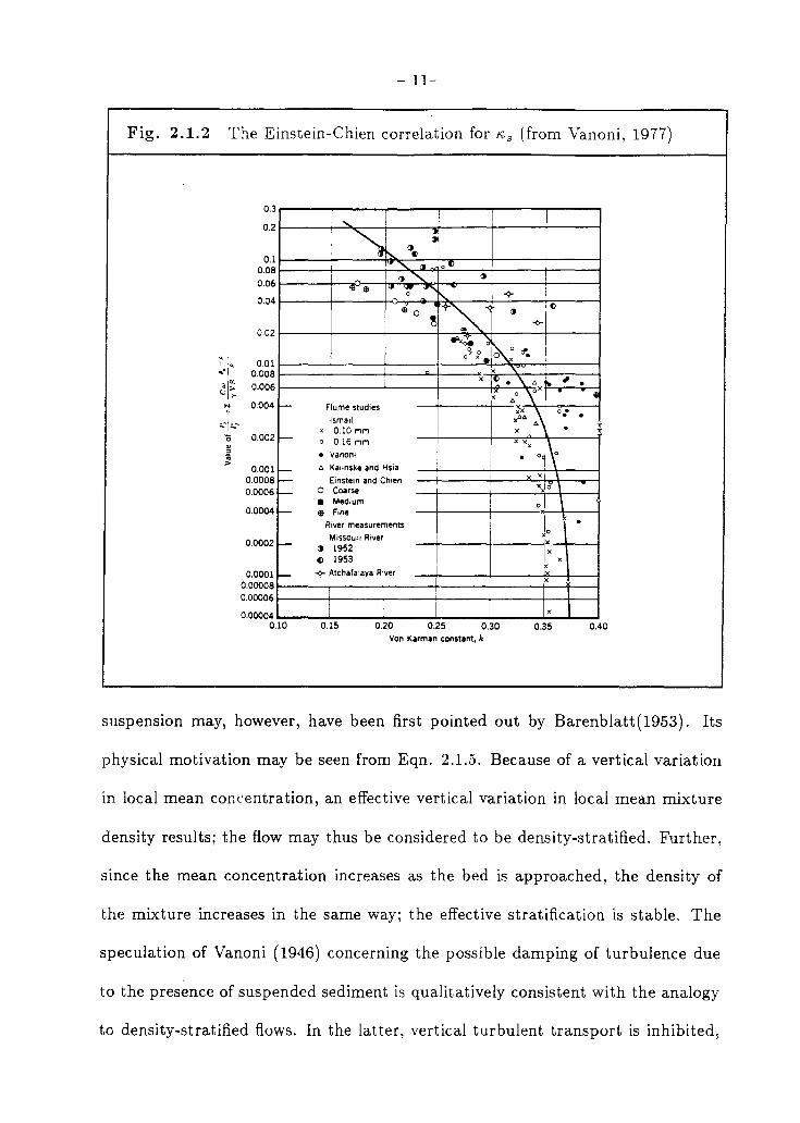
density-stratified flows. The correlation is reproduced in Fig. 2.1.2. Although
a crude trend may be discerned, a large scatter is evident, with values of P s / Pf
differing by an order of magnitude being associated with the same value of I'i., (or
l'i.,s in our notation). Although the quality of the data is uncertain, the fact that
l'i.,s attained values less than 0.2, nevertheless, indicates that a significant effect is
due to the presence of sediment. In the development of this correlation, however,
the appropriateness of a variable l'i.,s or even Eqn. 2.1.2 was not questioned. A
possible explanation for the large scatter is that, at least in some of these flows,
Eqn. 2.1.2 was inadequate.
If the traditional approach is considered as more than an empirical fitting
procedure, then it implies a qualitative view of the effects of sediment on the
turbulent flow. Since the log law is presumed valid throughout the flow, a reduction
in the von Karman constant affects the velocity profile throughout the flow. The
effects of the sediment, according to the tradit ional view, are global in nature.
In the western literature, the possible importance of a buoyancy effect was
already pointed out by Barton and Lin (1955). They noted that the Einstein-Chien
parameter, although not originally intended as such, could be interpreted as a
Richardson number. The meteorological analogy also inspired the analysis of Hino
(1963), who developed an analytical expression for the variation of l'i.,s from mixing
length concepts. The explicit analogy between thermal stratification and sediment
Page 31
- 11-
Fig. 2.1.2 The Einstein-Chien correlation for "'s (from Vanoni, 1977)
0.3
" 0.2
~ ~ I I
1 0.1 I ~ ~tl
0.08 .:-.. .Jl. 0" 0.06 ()' ()I
.. e 1- ";" "'r-. ~ 0.04
<Do ~r~~i ()
()
-1-0.02
:t~~ ~. I
~ IQ. 0.01 ~'I 0.008 ....0. x , I~\~
x () • "\ " ,
0.006 ~x ~o \x .
i ... 0.004 I- Flume studies ~ ~ " 0.- .
Ism.,1 ,,06 '-·I .. ~ 6 x 0.10 mm x
"0 0.002 I- 0 0.16 mm x Xx
01\ '" ~ • Vanont ;; . >
'" Kalinske and Hsia 0.001 t-0.0008 I- Einstein and Chien " x
0.0006 t- O Coarse x 10' \
• Medium 0 \ 0.0004 t- $ Fine
River measurements 10 0.0002 t-
MiSSOUri River
I: x (J 1952 tl 1953
x 0.0001 t- -1- Atchalalaya River
0.00008 x
0.00006 I
0.00004 0.10 0.15 0.20 0.25 0.30 0.35 0.40
Von Karman constlnt, k
suspensIOn may, however, have been first pointed out by Barenblatt(1953). Its
physical motivation may be seen from Eqn. 2.1.5. Because of a vertical variation
in local mean concentration, an effective vertical variation in local mean mixture
density results; the flow may thus be considered to be density-stratified. Further,
since the mean concentration increases as the bed is approached, the density of
the mixture increases in the same way; the effective stratification is stable. The
speculation of Vanoni (1946) concerning the possible damping of turbulence due
to the presence of suspended sediment is qualitatively consistent with the analogy
to density-stratified flows. In the latter, vertical turbulent transport is inhibited,
Page 32
- 12-
leading to a reduction in the scales of turbulent motion and a larger mean-velocity
gradient for given U x '
The explicit use of the Monin-Oboukhov formalism to describe particulate
turbulent flows appears in Monin and Yaglom (1971), Lumley (1976) and Itakura
and Kishi (1980), albeit with rather different definitions for the Monin-Oboukhov
length scale. Itakura and Kishi (1980) studied specifically open-channel flows with
alluvial sands and suggested that an appropriate Monin-Oboukhov scale would be
Ls == u~/[Kwsg(s-l)(c)l. The relation to the Einstein-Chien parameter is evident.
The log-linear velocity-defect profile proposed by Itakura and Kishi, based on their
Monin-Oboukhov approach, may be viewed simply as the use of a linear wake
function.
The straightforward application of the Monin-Oboukhov theory to sediment
laden open-channel flows faces several criticisms. The original theory was based
on constant, externally imposed momentum and scalar fluxes. The importance of
these assumptions lies in the possibility, for non-constant fluxes, of defining length
scales other than La, e.g., a local length scale based on dcldy, thereby invalidating
the simple similarity hypothesis that the mean profiles are functions only of (y I L s).
Since the momentum flux varies linearly with distance from the wall, the possible
importance of the depth, h, particularly if hi Ls ~ 0(1), as is often the case,
cannot be discounted. In the case of the sediment flux, this criticism has greater
force because of the large gradients often observed in sediment-concentration pro
files. An attendant difficulty is the definition of an appropriate Monin-Oboukhov
length scale. The wall heat flux, q*, in the atmospheric surface layer is assumed
externally imposed and constant. For the sediment-laden flow, little is known of
the concentration at the boundary; indeed, this is generally internally determined.
Page 33
- 13-
The use of \c) as a characteristic concentration may have little justification, since
the deviation of c(y) from (c) may be quite large. In this connection, Vanoni and
Nomicos (1960) argued that the Einstein-Chien parameter should be modified by
replacing (c) with a concentration close to the bed. This debate raises the question
of appropriate concentration scales in sediment-laden flow.
In contrast to the traditional view, the Monin-Oboukhov interpretation re
tains the universality of K and accounts for the deviation from the log profile by a
correction term, linear in Y/ L 8 • A similar argument has been advanced by Cole
man (1981), who proposed that the effects of suspended-sediment may be better
parametrized using the wake-function of Eqn. 2.1.4. Whereas in homogeneous
fluid flows, the wake-coefficient, Wo, has a constant value, say 0.2 in open-channel
flows, it may, according to Coleman, vary in sediment-laden flows. A correlation is
proposed between this coefficient and a gross flow Richardson number, defined as
Rc == gYmax(PO - PYm"J/(p)u;, where Ymax is the elevation where the maximum
velocity is found, Po and PYlllax are the mixture densities at Y = 0 and Y = Ymax,
and (p) is the depth-averaged mixture density. Of some practical relevance in the
use of this correlation is the difficulty in obtaining an accurate estimate of Po,
or equivalently, the concentration, co, at the bed. Coleman obtained estimates
by simple extrapolation, a dubious procedure in view of the large concentration
gradients near the bed.
Two conceptual points may be raised. The wake-coefficient characterizes
what may be termed the outer flow, i.e., the region where the wake function is
non-negligible. It is, however, correlated with a hybrid parameter, essentially
Ymax/LC = Ymax/(u:/g(s - l)co) in the context of sands, made up of an outer
length scale, Ymax, and a concentration scale, co, more characteristic of the inner
Page 34
- 14-
region. The resemblance to the Einstein-Chien parameter as modified by Vanoni
and Nomicos (1960) should be noted. This hybrid parameter may be justified if Co
is the only concentration scale, much as U x is the only velocity scale. This remark
is clarified in the following chapter. The second point is related and concerns the
magnitude of Ric. As estimated by Coleman from his starved-bed experiments,
these attain values up to 200. If Ric is interpreted in analogy to density-stratified
flows, such large magnitudes indicate extremely stable flows, in which turbulence
should be practically extinguished. This is evidently not the case, as shear must
remain important in order to sustain the suspension. The relation to the first point
is seen in that one reason for the large magnitudes is the use of Co as a concentration
scale. Alternate scales, e.g., (c), would result in much smaller values of Ric.
Conceptually, both the approach of Itakura and Kishi (1980) and that of
Coleman (1981) are identical, differing only in the specific wake functions and the
specific correlations (or equivalently, length scales) used. They both argue that, in
the region, y / Ls ~ 1 or y / Lc ~ 1 (presumably, y / h ~ 1 also), boundary shear
dominates and the effects of stratification are negligible, with the result that the
flow in this region should resemble a clear-water flow. In particular, the velocity
gradients in this region should be the same for both clear-water and sediment-laden
flows if u* is constant. Only in the outer region, y/L s = 0(1} or y/Lc = 0(1)
(and y/h = 0(1)}, are the effects of stratification felt. The effects of sediment
may therefore be considered localized in that they should be observed only in the
outer region.
Whether the velocity profile is best represented by a pure log law with Ks < K,
or with a log-wake law (where the wake function may be either linear or cos 2)
with a variable wake-co(lfficient, is still being debated. In spite of some qualitative
Page 35
- 15-
similarity such as the idea of turbulence damping, the traditional and the more
recent approaches ultimately diverge. The former's use of a pure log law with a
variable Ks implies a view in which the structure of turbulence is changed radically
throughout the flow. In the latter's view, the suspension affects primarily the outer
flow, such that, near the bed, where the wake function is insignificant, the structure
of turbulence remains essentially unchanged from that of a clear-water flow.
2.1.3 Sediment-laden flows: the mean-concentration profile
The mean-concentration profile is also to be determined in the sediment-laden
flow problem. The traditional view has not been seriously challenged. This view
has been based on the equation,
-c'v' + w c - 0 s - , (2.1.9)
found, for example, in Monin and Yaglom(1971), LumleY(1976) , and Vanoni(1977).
One interpretation of this equation is that it expresses the balance between the
net turbulent upward flux of sediment and the downward flux due to gravitational
settling.
The difference is noted between Eqn. 2.1.9 and the equation governing the
temperature field in the atmospheric surface layer, i.e., the problem for which
the Monin-Oboukhov theory was originally developed. In that case, the relevant
equation is
T ' , - v = q~, (2.1.10)
where T' is the fluctuating temperature. Whereas Eqn. 2.1.10 provides an unam-
biguous temperature scale because q* is constant, Eqn. 2.1.9 provides no intrinsic
scale for c. Further, the relevant momentum equation is -u'v' = u: (i.e., the same
Page 36
- 16-
as Eqn. 2.1.1 for y / h « 1). The similarity between momentum and temperature
equations suggests that the mean-velocity and temperature profiles are similar, as
indeed they are found to be. In the contrasting case of sediment-laden flows, the
difference between the concentration equation, Eqn. 2.1.9, and the momentum
equation, Eqn. 2.1.1, points to a radical difference between concentration and
velocity profiles. The difference in the structure of the governing equations is an
indication that sediment-laden flows may differ substantially from flows treated
by the Monin-Oboukhov theory.
The closure problem posed by Eqn. 2.1.9 may be resolved by a mixing-length
hypothesis (Lumley, 1976; Vanoni, 1977). Unlike the model for the velocity profile,
namely, -u'v' = {lmdu/ dy)2 = u;, where 1m = KsY is the mixing length, the model
traditionally used for the concentration profile is the somewhat inconsistent
_ ' '-!3 (1 dU)2 dc/dy c v - s m dy du/ dy
2 dc/dy = !3su.(l - y/h) / '
U", KsY (2.1.11)
where !3s is the reciprocal of a turbulent Schmidt number. Thus, the actual stress
profile, rather than the constant stress profile of the velocity model, is used. It
may be noted that some have suggested, on empirical grounds, using the actual
stress profile for the velocity model also (Montes and Ippen, 1971; Bradshaw, 1976;
Schlichting, 1979). The result of the traditional model is the Rouse suspended-load
equation (Rouse, 1937);
c (l- Y/h a/h )ZR
y/h 1-a/h ' (2.1.12)
where the Rouse parameter is defined as ZR == ws/ !3sKU", , and Ca is a reference
concentration at an elevation, y = a, where a is often taken to be a = O.OSh. Like
Page 37
- 17-
the log law, this solution cannot be valid at y = 0, since it predicts an infinite
concentration. A satisfactory answer to the question of the lower limit of validity of
Eqn. 2.1.12 has yet to be given, the most well-known being perhaps the suggestion
of Einstein (1950) that this should be within a few grain-diameters from the bed.
It has been implicitly recognized that Eqn. 2.1.12 does not adequately agree
with experimental results. In practice, it is used mainly to describe the profile in
the lower part of the flow, it being argued that the sediment concentration, and
hence the error, is often negligible in the upper part of the flow. Nevertheless,
more recent work that have emphasized the the two-layer nature of the problem
may be seen as attempts to improve on the traditional model. Constant eddy
diffusivities in the outer flow have been recommended by Coleman (1969) and van
Rijn (1984) on purely empirical grounds. The latter proposed a composite eddy
diffusivity in which the traditional eddy diffusivity is used below y / h = 0.5, and a
constant eddy-diffusivity is used above, with the constraint that it be continuous
at y / h = 0.5. Thus, in the upper half of the flow, the maximum eddy diffusivity
of the traditional model is used. If the estimated Z R for the van Rijn model and
the traditional model are the same, the former predicts larger concentrations in
the upper half of the flow than the latter. In the van Rijn model, the reference
level is distinct from the dividing line between the inner and the outer flow and is
situated near the bed.
A multiple-scales model may also be approached via scaling arguments. It
has been argued (Batchelor, 1965; Lumley, 1976; McTigue, 1981) that, near the
bed, the only relevant velocity scale is u., and the only relevant length scale is
y. The eddy-diffusivity of vertical sediment transport, Es , must then scale ·like
Es ,..., u",y, with the result that the solution near the bed is a power law. Note
Page 38
- 18-
that Eqn. 2.1.12 reproduces this in the limit, y/h« 1. McTigue(1981)' following
Batchelor(1965), suggested further that the only relevant scale in the outer flow
is h. Thus, Es ,....., u~h, i.e., a constant eddy diffusivity.
The analogy with density-stratified flows, previously emphasized in connec
tion with the velocity profile, has not yet had any significant impact on the
treatment of the concentration profile. Itakura and Kishi (1980), in their Monin
Oboukhov approach, simply used an eddy diffusivity based on their suggested
velocity profile. This seems contrary to the spirit of the similarity approach of
the original Monin-Oboukhov theory, in which the temperature profile is obtained
with an argument parallel to that used to obtain the velocity profile, without
invoking any eddy-diffusivity models.
A more thorough going interpretation in terms of the stratified-flow analogy
is found in the theory of Barenblatt(1979) (also cited in Monin and Yaglom, 1971).
This differs in several respects from the traditional approach and motivates some
of the ideas to be developed in the next chapter. A system of five equations,
including Eqn. 2.1.9 and a turbulent kinetic energy balance in which the stratified
flow analogy is explicitly made, is examined. The analysis is limited to the case
where the flow has absorbed the maximum possible amount of sediment. A general
solution to the system is not sought; rather, it is asked whether and under what
conditions self-similar solutions are possible. Such solutions are found possible
provided ws/ ",u .. < 1 (note "', and not "'s, is used in this criterion). The self
similar velocity profile is found to be logarithmic with what may be interpreted as
an effectively reduced "'s, while the corresponding concentration profile is a power
law profile with exponent, -1. It is argued that these are the only possible self
similar solutions. These solutions imply that the self-similar state is characterized
Page 39
- 19-
by a constant flux Richardson number, [g(s - l)c'v'JI[u'v'(du/dy)]. A constant
flux Richardson number is also found in flows treated by the standard Monin
Oboukhov theory; these are, however, highly stable rather than weakly stable
flows.
As a heuristic balance equation, Eqn. 2.1.9 may be satisfactory; whether it can
be justified more rigorously has been questioned. In an experimental study using
the LDV technique, van Ingen(19S1) was prompted to ask whether any physical
meaning can be attached to the correlation, -C'V ' , representing the net upward
turbulent flux of sediment. This questions the blithe acceptance of the continuum
assumption. Hinze(1972) notes that this assumption places severe restrictions on
a problem; in particular, the average separation distance between particles should
be at least an order of magnitude smaller than the Kolmogorov length scale,
lK = (V3/e)1/4, where e is the rate of turbulent kinetic energy dissipation. The
additional assumption of diluteness imposes even more severe restrictions. Since
the typical sand-grain diameter is of the order of or greater than 1 K, the continuum
assumption in sediment-laden flows of rivers should not be taken lightly.
Over what length scales is it possible to define a concentration? LumleY(1976)
estimates that, for an accuracy of 10% in the definition of a local particle density,
3000 particles in a characteristic volume are necessary. For a fairly high concen
tration of 0.005, and a grain diameter of 0.15mm, this requires a characteristic
volume of ~ 1cm3 . In the laboratory where lK -- O.lmm, the length scale over
which a concentration can be defined is significantly larger than lK. Because the
fluctuating concentration field can be defined only on scales much larger than the
significant scales of the fluctuating velocity field, the correlation, -C'V' , has ques
tionable physical meaning in the context of alluvial sediment-laden flows. Thus,
Page 40
- 20-
the effort, made for example by mixture theorists (Drew, 1975; McTigue, 1981),
to derive equations like Eqn. 2.1.7 using continuum-type assumptions in which
correlations between concentration and velocity fluctuations appear, seems inap
propriate for this particular class of problems. The difficulty may be avoided, as in
the approach of Batchelor (1965), who started directly from a gradient-transport
model without reference to any correlations. The gradient-transport assumption
is, however, itself not above question.
2.2 Experimental results
2.2.1 Mean-field results
In the literature on open-channel flows without sediment, the limitations of
the purely logarithmic velocity profile and the necessity for a wake-type correction
have become increasingly apparent. The specific wake-function of Coles (1971)
appears to be gaining wide acceptance. There is wide scatter, however, in the
reported values of the Wo, ranging from 0 to 0.25 in experiments of Nezu and
Rodi (1986), and from 0 to 0.48 in results examined by Coleman and Alonso
(1983) .
In the investigation of the velocity profile in sediment-laden flows, a number
of experimentally-related factors contribute to the controversy between traditional
and recent approaches. An accurate estimate of the wall shear, independent of
any assumptions about the velocity profile, is complicated by a finite width and by
differences in the roughness of the bed and the sidewalls. Since the determination
of K (or Ks) depends on u*, this introduces error in the estimate of K, Exper
imental procedure plays a role also in that, a velocity profile is often obtained
from a relatively small number of points (8-12). The performance of the standard
Page 41
- 21-
instrument, the pitot-static probe, in proximity to solid boundaries has also been
a source of doubt.
The criticism of Coleman (1981) with respect to the early practice of fitting
a logarithmic curve to the entire flow is justified. Re-examination of the early
work reported, e.g., by Vanoni(1946) and Vanoni and Nomicos (1960), shows that
measurements made very near the bed were weighted less in the fitting of the
logarithmic profile. If these had been given more weight, the estimates of /\'$ would
be typically revised upwards. In a re-examination of some data of Vanoni (1946),
Coleman determined a/\,= 0.5 by fitting the logarithmic curve to the near-bed
measurements in both a clear-water and a sediment-laden flow. In their defense,
this early practice may reflect an implicit judgement of the reliability of near-bed
measurements, which, from the high value of /\, found for even a clear-water flow,
may be well founded. The justice of Coleman's criticism does not necessarily
invalidate the traditional hypothesis, although it certainly throws doubt on it.
The experiments on which Coleman(1981) based his wake-function correla
tion may, in turn, be criticized for the small width-to-depth ratio of 2. Three
dimensional effects due to the sidewalls may be important. Such effects would
be of greatest importance in the outer flow, precisely the region in which it is
claimed that the effects of the suspension are primarily felt. Two points may,
however, be noted. The aspect ratio was kept approximately constant in all of
his experiments, so that the effects of the sidewalls should be approximately the
same in all the experiments, unless these effects depend strongly on sediment con
centration. Also, the few near-bed measurements, which should be less influenced
by three-dimensional effects, indicated a value of /\, ~ 0.4, which was independent
of sediment concentration. Nevertheless, the reliability of near-bed measurements
Page 42
- 22-
with a pitot-tube and the statistical significance of a logarithmic fit over two or
three points is questionable.
Although less controversy has surrounded the concentration profile, similar
experimental problems exist. The traditional suction-sampling technique intro
duces a sampler into the flow. In an equilibrium-bed flow, the reliability of near
bed measurements is uncertain because of possible local local scour of the bed
induced by the sampler. Even in starved-bed flows where this is not a problem,
measurements cannot be made at the bed because of the finite size of the sampler.
The accuracy in measuring local mean concentration that may be expected of such
a technique is, perhaps at best, 10%, compared to an accuracy of perhaps 1% in a
mean-velocity measurement. The tedious procedure has probably also contributed
to the fact that fewer data are available on point concentrations.
As noted earlier, it has been traditional practice to place more weight on
near-bed measurements in trying to apply the Rouse equation, Eqn. 2.1.10. This
may have again reflected concern about the reliability of measuring the small
concentrations in this region, and also possible effects of a slight non-uniformity of
the grain-size distribution. The evidence presented in support of the more recent
approaches has been rather meager. Both Itakura and Kishi (1980) and McTigue
(1981) gave a comparison of theory and experiment for only a single experiment.
The experimental evidence regarding the mean profiles may therefore be con
sidered inconclusive with both traditional and recent approaches open to criticism.
The possibility should not be ruled out, particularly with respect to the velocity
profile, that both approaches may be valid, each for a different range of conditions.
2.2.2 Results on the fluctuating velocity-field
One of the earliest studies of the fluctuating velocity field was reported by
Elata and Ippen (1961), who used an impact-tube pressure transducer to measure
Page 43
- 23-
longitudinal velocity fluctuations in a flow transporting neutrally buoyant particles
of a single size. They reported a decrease in "'8 (which has since been questioned
by Coleman (1981)), and an increase in turbulence intensity with increasing par
ticle concentration. They, therefore, disputed the speculation of Vanoni (1946)
that the presence of sediment damped turbulence, and suggested that the struc
ture of turbulence was altered by the presence of the additional solid surface of
the sediment. The major effect was, nevertheless, obtained in flows with volume
concentrations (up to 0.3) an order of magnitude or more larger than those to be
considered in the present work. Particle-particle interactions would undoubtedly
be of more significance in their work. These experiments could also be criticized
for the non-uniformity of the flow.
Smaller concentrations, up to 0.03, of slightly negatively buoyant particles
were again studied by Bohlen (1969), who measured the three velocity compo
nents in a silicone-oil, open-channel flow using hot wire probes. While his results
showed the same trend with increasing concentration as those of Elata and Ippen
(1961), the magnitudes of the measured intensities may be questioned. Typically,
as the wall is approached, the following scaling is usually found: v;;J2 / u,. '" 2,
~/U,. > ~/u* '" 1. Bohlen's data, including a particle-free flow, conSIS
tently showed all turbulence intensities to be less than u",.
The LDV technique offers an alternative that avoids the difficulties of intro
ducing a physical probe into the !low. The work of van Ingen (1981,1983a) investi
gated a sediment-laden, open-channel flow with a predominantly fiat equilibrium
bed. A single sand size was used, and only the longitudinal velocity component
was measured. A slight increase in ~ / u, compared with clear-water flow, was
observed. It was cautioned, however, that the slight increase in ~/u might
Page 44
- 24-
not be statistically significant in view of the scatter in results reported by other
workers. Tsuji and Morikawa (1982) used a single-component LDV technique also
in studying air flow in a pipe, with a suspension of particles of two sizes. They did
not, however, analyze velocities in terms of the log-law. Longitudinal turbulence
intensities relative to the bulk mean speed, v;J2 / (u), were found to decrease with
increasing concentration of small particles, d = O.2mm (pipe diameter, 30.5mm),
and to increase for large particles, d = 3.4mm. The implications of this study for
the present work are not clear in view of two essential differences between particu
late airflow in a pipe and sediment-laden open-channel flows, namely, the density
ratio and the geometry.
2.3 Summary
Both the traditional and the more recent approaches to the description of
the two mean ~elds and to the interpretation of experimental results are open
to criticism. The recent more explicit analogy to density-stratified flows in the
treatment of the velocity profile has been discussed. A trend away from a reliance
on the the mixing-length closures towards the adoption of an approach based more
on similarity ideas may be seen in the application of the Monin-Oboukhov theory
and, to a lesser extent, in the wake-coefficient correlation.
In contrast, both the traditional and the more recent treatments of the con
centration profile remain tied to a vertical balance equation, whose conceptual
foundations have been questioned. The stratified-flow analogy has been seen to
have had little impact. This asymmetry in the conceptual approach to the descrip
tion of the two mean fields may be attributed to the traditional implicit decoupling
of the velocity from the concentration field. In the next chapter, an attempt is
made to follow more systematically and thoroughly a similarity approach, which
treats the two mean fields in parallel but different ways.
Page 45
- 25-
3. Similarity and sediment-laden flows
3.0 Introduction
The preceding review highlighted the controversies surrounding the descrip
tion of the mean fields. To clarify some of these issues and to develop an alternative
conceptual framework for thinking about sediment-laden flows, a discussion of the
concepts of self-similarity, multiple scales, and asymptotic matching is given. The
similarity approach to wall-bounded turbulent shear flows can be formalized in an
argument originally given by Izakson (1937) and Millikan (1939). An outline of
the conventional argument, following Tennekes and Lumley (1980), is given. Since
the concepts of multiple scales and asymptotic matching are important in homo
geneous flows, it is natural to ask to what extent they apply to sediment-laden
flows. If these concepts may be applied to the velocity profile in sediment-laden
flows, how do they apply to the concentration profile? A naive generalization of
the conventional matching argument to the case of the concentration profile con
cludes that the profile follows a logarithmic law 0 This is contrary to experimental
evidence. A more appropriate generalization is developed such that asymptotic
matching may result in either a power law or a log law. A two-stage similarity
model for sediment-laden flows is then developed, using this generalization.
Page 46
- 26-
The discussion regarding sediment-laden flows is restricted to a simplified
case. Unless otherwise specified, a suspension in equilibrium with a sand bed is
assumed. The bed itself, though deformable, is assumed to be flat and statistically
stationary, and to be composed of sand grains perfectly uniform in density and size.
Temperature effects are not considered. All variables are assumed homogeneous
in the streamwise direction.
3.1 The conventional matching argument
A general law of the wall may be expressed as
(3.1.1)
where y+ == y/lv, Lv == v/u*, and O:i is a dimensionless parameter, relevant only
in the inner region, e.g., a roughness Reynolds number, Rek == k/lv, k being the
characteristic height of the roughness element. Similarly, a general velocity-defect
law is considered, namely,
u - U max (3.1.2)
where TJ == Y / h, and 0: 0 is a dimensionless parameter relevant only in the outer
region, e.g., the bulk Richardson number proposed by Coleman (1981). Following
Tennekes and Lumley (1980) and the standard practice in multiple-scales analysis
(Kevorkian and Cole, 1981), we consider the inner variable, y+, and the outer
variable, TJ, to be essentially independent. An asymptotic matching of the velocity
gradients is then proposed. From Eqn. 3.1.1,
du
dy
u. df
z: dy+' (3.1.3)
Page 47
while from Eqn. 3.1.2,
du
dy
- 27-
u.dF h d17'
(3.1.4)
In an intermediate region, y+ -----+ 00, 17 -> 0, Eqns. 3.1.3-3.1.4 are assumed to
match asymptotically, such that
(3.1.5)
Multiplication by y /u* then reveals
dF + df 17 d17 = Y dy+' (3.1.6)
For given parameters, a o and ai, the two sides of Eqn. 3.1.6 (which should, strictly
speaking, be interpreted as an asymptotic relation) depend on different variables
and so must be equal to a constant, independent of 17 or y+. This matching con-
stant, traditionally denoted by 1/ I'i-, is independent of either aa or ai, since these
are relevant only in their respective regions. In this limited analysis, the matching
constant is universal in the sense that the asymptotic limit, Re", == h/lv --jo 00, has
been taken in obtaining the constant, such that it must be independent of Re".
The matching solution in the intermediate region, tv « y « h, is obtained by
integrating Eqn. 3.1.6 to give, in inner coordinates,
(3.1.7)
where the constant of integration, B i , may depend on ai, but not on Re",. Simi-
larly, in outer coordinates, the matching solution is expressed as
(3.1.8)
Page 48
- 28-
Although the above analysis considered the special case where the inner length
scale is ll/' nothing in the analysis depends on this choice. The same result would
be obtained for any other inner scale, l, provided that the disparity in scales exists.
Further, the matching constant should remain the same. Consider a case where
lv « l « h, and matching occurs in l « y « h, with a matching constant,
1/ /\,'. If l decreases, the matching constant does not vary. In the asymptotic
limit, where l/lv ~ 0(1), matching can be obtained with either y+ or y/l as the
inner coordinate, so that the matching constant must be the same, i.e., 1/ /\'. A
familiar example is the case of flow over a fully rough surface, in which case, k is
the appropriate inner scale rather than lv, and a /\, ~ 0.4 still characterizes the
logarithmic velocity profile.
What conclusions can be drawn in a case where a dimensionless parameter, &,
that is relevant in both inner and outer regions exists? The above matching anal
ysis can still be applied but a "universal" matching constant cannot be deduced.
The possibility that the matching constant varies with this parameter cannot be
excluded.
3.2 A generalization of the conventional matching argument
The traditional approach to describing the mean-concentration profile has
been based on the balance equation, Eqn. 2.1.9, and an eddy-diffusivity modeL
Since similarity laws are familiar in the context of the velocity field, can such sim
ilarity concepts provide an alternative framework for discussing the concentration
profile? In particular, are there equivalents to the law of the wall and the velocity
defect law for the concentration field? Can a matching argument be found to de
duce a plausible concentration profile in some matching region? The conventional
Page 49
- 29-
matching argument is not restricted to the velocity field but can be applied to any
dependent variable. A straightforward application of the conventional matching
argument with concentration instead of velocity as the dependent variable yields
a logarithmic profile for the concentration profile in the intermediate matching
region. This is not a trivial result, since the temperature field in a weakly stable
atmospheric surface layer, as treated by the Monin-Oboukhov theory, exemplifies
this result. Such a logarithmic behavior is not observed in sediment-concentration
profiles. The conventional matching can, however, be formally generalized in a
heuristic manner such that it admits not only log-law profiles but also power-law
profiles in the matching region.
Assume that two disparate length scales, land £, exist and are important in
two distinct flow regions, i) yjl = 0(1), yj £ « 1, and ii) yjl ~ 1, yj £ = 0(1).
A general inner law for a dependent variable, r, may be expressed formally as
(3.2.1)
where r * is an appropriate scale. An outer law can be similarly expressed as
(3.2.2)
The scale, r * is assumed to be common to both regions (like u *). As in the con-
ventional argument, the variables, ~ == y I land", == y 1£, are treated as essentially
independent in the asymptotic limit, £Il -+ 00. With a view to matching the
gradient, Eqns. 3.2.1-3.2.2 may be differentiated with respect to y to give
dr [la! 1 ail (3.2.3) - = r. T a~ + £ aTl ' dy
and
dr [1 aF 1 aFl (3.2.4) dy = r. T a~ + £. a", .
Page 50
- 30-
These are to be matched in an intermediate region, e -+ 00, ry -+ 0, such that
1al 1al 1aF laF I a~ ~ L ary = I a~ + L ary . (3.2.5)
Multiplication by y converts this asymptotically valid equation to a relation ex-
pressible in terms of only ~ and ry, i.e.,
(3.2.6)
The conventional argument relies on the separability of both sides of Eqn. 3.2.6;
both I and F should be such that the operation, T<I>, where T == ~a/a~ + rya/ary,
results in a separation of variables. If this were the case, then division by the
appropriate factor would result in an equation of expressions, each of which is
dependent on its own variable and so must be constant. A class of particular
solutions which may be useful is found where I (or F) is itself separable; i.e.,
I = Id~)h(ry)· (3.2.7)
This results in
(3.2.8)
From this, it is clear that the separability condition is that
(3.2.9)
where Al is an undetermined constant, with the simple solution
(3.2.10)
Instead, therefore, of the general relations, Eqns. 3.2.1-3.2.2, we assume that
!...- = ryAl <I>r(e) , r~
(3.2.11)
!...- = E"' 2 <I>2(ry). r.
(3.2.12)
Page 51
- 31-
The form of Eqns. 3.2.11-3.2.12 was chosen such that the special case treated by
the conventional argument is included when Al = A2 = O. The matching condition,
Eqn. 3.2.5, then results in
(3.2.13)
where C 1 is the matching constant. The general equation to be satisfied by ~1
and ~2 is of the form
(3.2.14)
In the special case where Al = A2 = 0, the classical result is obtained. The general
solution of Eqn. 3.2.14 is
(3.2.15)
where C~ = CI/(Al + A2)' In the overlap layer, the profile may, therefore, be
expressed in terms of inner coordinates as
(3.2.16)
This may be put in more insightful form by defining a new scale for the inner
region, re = r. (1/ £) .. 1 j and denoting (AI + A2) as A, with the more compact
result,
In a similar fashion, with the additional definition, r" _ r .. (£. / l) .. 2, the outer-
solution form of the profile in the overlap layer is
r I).. - = C l l1 + C3 •
r" (3.2.18)
Page 52
- 32-
Not surprisingly, the form of Eqn. 3.2.18 is similar to the classic log law with the
substitution of the power-law for the log-law. A significant difference, however, is
that, rather than having a common scale, as first assumed, for both the inner and
outer layer, two disparate scales are found to be necessary. Since the dependent-
variable scales must satisfy the relation,
(3.2.19)
and it is assumed that I ~ ;::" these must be disparate scales, unless>.. = 0, as in
the conventional argument.
The development, though formal and heuristic, is quite general in that it does
not depend on any particular inner or outer scales but requires only that the inner
scale and the outer scale are disparate. Moreover, although the discussion has been
in the context of wall-bounded flows, it may be applied much more generally. Thus,
results for the downstream evolution of free turbulent flows such as buoyant jets,
as well as for other wall-bounded turbulent flows, such as a turbulent boundary
layer on the verge of separation, may be viewed from this general perspective. The
classic logarithmic profile is thus seen as a special degenerate case in which only
a single velocity scale is relevant for both inner and outer regions, imbedded in a
much broader range of profiles.
The remarks previously made in the context of the log-law profile should also
apply to the power-law profile. In particular, if a dimensionless parameter, /3, is
relevant in both inner and outer regions, then all of the the constants involved
in the profile, including the exponent, >.., may vary with this parameter. It is
implied here that any such dimensionless parameter must remain finite in the limit,
f. / I ~ 1. In this connection, the power-law profile may be interpreted generally
Page 53
- 33-
as an example of what Barenblatt and Z'eldovich (1972) have termed "self-similar
solutions of the second kind" (also Barenblatt, 1979). The exponent, A, may be
regarded as an eigenvalue in the sense that only for certain values of A can the
inner and outer solutions, which are determined by the boundary conditions, be
matched. In cases where closed equations can be investigated analytically, e.g., the
Guderley solution of the blast-wave problem in gas dynamics (Whitham, 1974),
the eigenvalue aspect of A is revealed clearly. In that example, A is seen to possess
a continuous spectrum that depends on the ratio of specific heat capacities, a
dimensionless parameter relevant on both sides of the singular characteristic.
3.3 Another approach to a generalized matching argument
Another approach to the conventional argument, closer to the original treat-
ment, is preferred by some workers. This approach, exemplified by that taken in
Monin and Yaglom (1971), may also be used to obtain an equivalent generalized
matching argument. Although it leads to a less general result, it is convenient to
assume, from the start, a disparity in scales. We begin, therefore, with
~ = f{E), Te r
- = F{rl) , Try
(3.3.1)
(3.3.2)
and ask under what conditions these can be matched? In the overlap region, r is
assumed to match, so that
(3.3.3)
where "I == £/1. Letting
(3.3.4)
Page 54
- 34-
gives a functional equation for g,f, and F,
g(J)f(rrd - F(l7) = O. (3.3.5)
Taking the derivative with respect to /, we obtain
(3.3.6)
Multiplication by / reveals the possibility of separation of variables such that
xJ'(x) = A f(x) , (3.3.7)
where A is the separation constant, and the group, 17/, has been relabelled as x.
The solution of Eqn. 3.3.7 results in a power law as expected. Note, however, that
there is no additive constant, differing from the previously obtained result. This
is a consequence of the assumption of disparate scales from the beginning.
Eqn. 3.3.7 for f may be expressed in terms of the original variables, rand y,
as
~ dr = A. r dy
(3.3.8)
A familiar physical argument in the context of the velocity profile and the log law
is that there exists a region in which y is the only relevant length scale. From the
perspective of multiple scales, this may be more precisely stated as the existence of
a region, 1 « y « .£. In the case of a power law, we may say that, in addition, in
this same region, r itself is the only relevant scale, or more precisely, r e « r « r 77'
Eqn. 3.3.8 is then interpreted as an extension of the familiar scaling argument
rather than arising from a matching argument.
Page 55
- 35-
3.4 Implications for sediment-laden flows
3.4.0 Introduction
It has been shown that a power-law profile with a variable exponent, as well
as the conventional logarithmic profile, may be deduced from general assumptions
regarding the existence of similarity laws and of disparate scales. The Rouse
suspended-load equation, Eqn. 2.1.12, tends asymptotically, as rJ --+ 0, to
--ZR C"'rJ , (3.4.1)
i.e., a power law with a variable exponent. This suggests that the arguments of the
preceding sections may be used to obtain a description of the mean-concentration
profile without appealing to either a vertical balance equation, a mixing-length or
an eddy-diffusivity hypothesis. Can similarity concepts provide a flexible alterna, tive as the basis of a conceptual framework? What assumptions are necessary for
such an approach to give plausible results? An answer to this question is developed
in two stages. Basic similarity hypotheses are stated in the first stage and their
implications developed. At this stage, specific physical content is minimized by
not specifying length and concentration scales. The implications remain general
and compatible with a variety of more specific physical models. At the second
stage, we consider two specific models as embodied in part£cuiar choices of length
and concentration scal~s, one corresponding to the analogy to stably stratified
flows, and the other motivated from a more general dimensional analysis.
3.4.1 Similarity hypotheses and implications
The following basic hypotheses are made:
HI. A two-layer structure exists in which an lllner region of extent, is, can be
distinguished from an outer region, whose scale is the depth of flow, h.
Page 56
- 36-
H2. As far as the velocity profile is concerned,
a) a single common velocity scale, u., characterizes both the inner and the
outer regions, and
b) no dimensionless parameter is relevant in the outer region.
H3. As far as the concentration profile is concerned,
a) two disparate concentration scales, Cs and Ch, exist, and
b) a dimensionless parameter,~, is relevant in both the inner and the outer
reglOns.
H4. In each region, asymptotic similarity In the inner and the outer variables
prevails.
In mathematical form, these may be stated in terms of inner similarity laws;
U - = f(es; (Xi), U",
(3.4.2)
C A
- = g( es; {3, (3i), Cs
(3.4.3)
and of outer similarity laws;
U - U max (3.4.4)
(3.4.5)
From these fairly general yet restrictive hypotheses, what can be deduced?
If it is believed that the presence of sediment may noticeably affect the velocity
profile, then, from HI, it must be concluded that Is cannot be either 1/,1 or d50 •
Otherwise, the velocity profile would be essentially identical to the clear-water
case. This does not preclude the possibility that ILl or, more likely, d50 j may
be important in some region of the flow, e.g., very near the bed. The two-layer
Page 57
- 37-
assumption applies to the region of flow that we are interested in and which we
can investigate experimentally. It supposes then that other possible length scales
are much smaller than is. We also leave open the possibility that, under certain
conditions, the extent of the inner region may grow so as to render the inner region
indistinguishable from the outer region. This region of extent, is, may be loosely
interpreted as that to which the effects of the presence of sediment are confined.
The possibility of a power-law velocity profile is eliminated by H2a, which
argues in favor of a logarithmic profile with an associated von Karman constant
of::::= 0.4, i.e., the same as in clear-water flows. It should be emphasized that, as is
made clear in the matching argument, such a profile is asymptotically approximate
for lsi h ~ I and should be observed only in a limited intermediate region, ls ~
y ~ h. If cases exist where ls '" h, then these simple hypotheses are no longer
sufficient to give a definite result; a logarithmic profile mayor may not be observed.
From H2b, it is deduced that the wake component of the velocity profile remains
the same as in clear-water flows. This is a simplifying hypothesis, which may be
relaxed.
The existence of two disparate concentration scales allows the possibility of a
power-law profile, as argued in the preceding sections. As in the case of the velocity
profile, such an asymptotic profile should be found only in a intermediate region.
The assumption in HI that only two length scales, is and h, are important in the
region under consideration implies that the inner length scales of the velocity and
the concentration profiles are the same. This may be motivated by the belief in a
strong coupling between the the mean- velocity and concentration fields. It may
also be viewed as a weak form of a Reynolds analogy between vertical sediment
and momentum transport. The existence of a dimensionless parameter, ~, that is
Page 58
- 38-
relevant in both inner and outer regions for the concentration profile only permits
the possibility of an exponent that may vary with this parameter.
From fairly general hypotheses, fairly definite conclusions have been drawn.
To some extent, these hypotheses were tailored to fit qualitative experimental
evidence. The description of the concentration profile by a power law with a
variable exponent, deduced from our hypotheses, has essentially reproduced the
traditional result in the asymptotic case, r] « 1, or that based on a direct eddy
diffusivity model with Es '" u,..y. In the case of the velocity profile, however, the
conclusions drawn differ significantly from those of previous approaches. It has
been argued that the effects of the presence of sediment may be confined to a
layer near the bed, of extent ls' The traditional model argues that these effects
are observed throughout the depth of flow. The more recent models based on the
stratified-flow analogy argue that these effects are primarily found in the outer
region of the flow. Although it can reproduce some old results, the proposed
approach is distinct from previous approaches. It is also more flexible in that it
recognizes the possibility of cases where effects of sediment may be felt throughout
the flow (Ls ,...., h).
Whether the hypotheses on which the similarity approach is based are any
less questionable or any more fruitful than previous hypotheses may be debated.
What we consider to be the advantages are that
i) there is no reliance on balance equations whose justification is questionable;
ii) there is no reliance on mixing-length or eddy-diffusivity hypotheses;
iii) the velocity and the concentration fields are treated in parallel as befits a
coupled problem, with no priority being assigned to the velocity field, the
Page 59
- 39-
coupling between the two fields appearing in a general way, in that a common
inner length scale is assumed;
iv) the assumptions, implicit in simple mixing-length models, and thus often over
looked, are clarified, e.g., the limited extent of the region where a logarithmic
profile should be observed, and
v) the use of a similarity treatment imbeds the sediment-laden flow problem in a
general scheme which has been used to treat a large number of other turbulent
flows.
3.4.2 A wake component in the concentration profile
The term "wake component" is a misnomer in the context of open-channel
velocity profiles because the strict analogy with a wake flow in the outer region
fails. More generally, the wake component may be interpreted, and is so inter
preted throughout this work, as reflecting the effect of the bounding free surface.
The spatial extent of such an effect is uncertain; experimentally, it is found in
clear-water flows that, above, say rJ = 0.2, the effect is noticeable in the velocity
profile. Because the origin of such an effect, as interpreted here, is so general, it
seems highly likely that a wake effect will be observed in sediment-laden flows.
Indeed, we have previously argued that, where lsi h « 1, the wake component for
the velocity field will remain largely unchanged in importance from that found in
clear-water flows.
Consistent with its presence in velocity profiles, a wake effect must also be con
sidered a possibility in the concentration profile. The matching argument makes
explicit that the power-law can be justified only for rJ « 1, and, presumably, be
comes increasingly invalid as rJ ---+ 1. The adoption of a constant eddy diffusivity
in the outer region may be viewed as an attempt to characterize better the wake
Page 60
- 40-
component. Instead of the traditional reliance on eddy diffusivity concepts, and
the use of the vertical-balance equation, a simpler approach, more consistent with
similarity concepts, is proposed. This is the use of a wake function for the con-
centration profile also, therefore paralleling the treatment of the velocity profile.
It is suggested that a general profile, valid for the matching and the outer regions,
be of the form,
C Z A
--rl- W(rl· a ) -'f "C\'"fJ"
Ch (3.4.6)
where We (17; ~) satisfies the asymptotic conditions,
as 17 -+ 0, (3.4.7)
as 17-1. (3.4.8)
This last condition, based on the grounds that the concentration should vanish at
the free surface, may be debated but is adopted for convenience. Eqn. 3.4.6 can
be expressed in a more suggestive form by taking the logarithm,
log c - log Ch 1 (A) Z = -log 17 + Z log We 17; (J . (3.4.9)
By analogy with the treatment of mean-velocity profiles, it IS proposed that a
useful form of the concentration wake function, We, may be
(3.4.10)
where the restricted wake function, W eO , is independent of the parameter, ~, and
Zh plays the role of a wake coefficient. Beyond this level of simplification, the
choice of Wco is arbitrary within the above asymptotic constraints. A particularly
Page 61
- 41-
simple choice of Wco that allows easy comparison with the traditional result IS
proposed; namely,
W co =(l-ry). (3.4.11)
Our general profile, valid for y / ls » 1, may be expressed as
C _ -z(l )Zh --ry -ry. Ch
(3.4.12)
This is seen to differ from the traditional suspended-load equation in at least two
important respects. A concentration scale with some physical significance replaces
the simple reference concentration. Secondly, the traditional model would insist
that Zh == Z, while the present approach permits the two exponents to differ. A
non-dimensional eddy diffusivity may be associated with the profile, Eqn. 3.4.12;
namely,
(3.4.13)
If Z is identified with Z R, the factor in square brackets distinguishes the present
from the traditional eddy diffusivity. Depending on whether Zh/ Z < 1 or Zh/ Z >
1, the former will be larger or smaller than the latter.
An alternate choice of Wco is such that
log Wco = ry, (3.4.14)
which leads to an exponential decay in the outer region and is consistent with a
constant eddy diffusivity in that region. This does not satisfy the condition given
by Eqn. 3.4.8.
3.4.3 An inner length scale for sediment-laden flows
It should be emphasized again that the above results rest on comparatively
few physical assumptions because the length scale, i Sl the concentration scales, Cs
Page 62
- 42-
and Ch, and the parameter, {3, have yet to be specified. In the present study, we
will not be concerned with the dimensionless parameters, D:i, {3i, since these are of
secondary importance. The above basic similarity structure is therefore compatible
with a variety of more specific physical models. The validity or invalidity of any
of the more detailed physical assumptions does not affect the validity of the basic
structure. To obtain more specific results, however, more specific assumptions,
which will determine the scales, are necessary.
Two familiar inner length scales for sediment-laden flows have been implicitly
or explicitly suggested by previous workers, namely, the viscous scale, Lv (Itakura
and Kishi, 1980; Coleman, 1985), and the grain diameter, dso (Einstein, 1950;
Elata and Ippen, 1961). The viscous scale is not peculiar to sediment-laden flows
and needs no further comment. As a possible inner scale, the grain diameter
presents a number of different aspects. At the simplest level, it provides a rough
ness height, which, again, is not peculiar to sediment-laden flows. It is also associ
ated with the concept of bed-load transport put forward by Einstein (1950), who
argued that a transitional layer with thickness scaled by dso exists between the
bed and the suspension. The grain diameter should thus be interpreted in terms
of a saltation height, characterizing the elevation to which a saltating particle
rises. Yet another interpretation of dso as length scale was offered by Elata and
Ippen (1961), in their study with neutrally buoyant particles. They argued that
neutrally buoyant suspended particles are capable of directly affecting turbulence
primarily at scales that are comparable to the particle size. Since typical grain
sizes are of the same order of magnitude as or larger than the Kolmogorov scale,
there would exist a range of scales within which interaction between sand grains
and turbulence may occur. Moreover, since smaller scales become more important
Page 63
- 43-
as the bed is approached, the effect of suspended particles should be primarily in
the flow near the bed. Another inner length scale, which was suggested by Cole
man (1969), may also be mentioned. It is the displacement thickness of the actual
sediment-laden channel flow. The motivation for this suggestion was not given and
the displacement thickness may be regarded as an ad hoc empirical scale. Even in
the theory of turbulent boundary layers where this length scale is of more use, it
is considered more of an outer scale than an inner scale being defined in terms of
an integral over the entire boundary layer.
Our viewpoint is closest in spirit to that of Elata and Ippen, which focuses
on the effect on turbulence and is consistent with a multiple-scales interpretation
of wall-bounded turbulent shear flows. We argue, however, that, in the case of
sedimenting particles with a non-negligible settling velocity, it is not clear that the
grain diameter remains the only important physical parameter, since the settling
velocity may be equally important or perhaps even dominant. Indeed, we have
already concluded from our basic similarity model that if the presence of sediment
does markedly affect the velocity profile, then dso cannot be identical to is.
A general relation between the physical parameters relevant in the inner region
may be expressed as
(3.4.15)
where is may be considered the dependent variable and the other parameters are
independent, externally imposed variables. It has been assumed that h is irrel
evant in the inner region, and so has been excluded from consideration. More
convenient forms of Eqn. 3.4.15 may be obtained by replacing one of the indepen
dent parameters by other equivalent parameters. In particular, since the standard
Page 64
- 44-
drag curve for a single sphere, falling under gravity at its terminal settling ve-
locity, WsO, in a stagnant flow, relates the parameters, g(s - 1), d50 , £/, and WsO,
then the latter may be substituted in Eqn. 3.4.15 for any of the other three. The
motivation for such a substitution stems from the use of a settling velocity, Wa
(to be distinguished from waO), in the traditional treatment of the concentration
profile. The inclusion of WaO in the "basis" parameters allows an easy comparison
with the traditional result. Because WaO is defined from the standard drag curve,
it unambiguously characterizes the particle and the fluid and is independent of the
flow. Its use as a "basis" parameter thus avoids the conceptual problem, encoun-
tered in previous approaches based on the flux of settling particles (e.g., in the
use of Eqn. 2.1.9), of determining the actual settling velocity, W a , in a turbulent
suspenSIOn. The latter would, strictly speaking, vary with local concentration as
well as on the turbulence intensity (at least).
In the case where la ::;p lv, it is reasoned that a more appropriate represent a-
tion of Eqn. 3.4.15 is
(3.4.16)
Viscous effects are thus assumed to be important in this inner region only insofar
as they affect the grains, and not as they arise from the bottom boundary. From
dimensional considerations, Eqn. 3.4.16 may be expressed as
= g(s - l)la =;::; (wao g(s - 1)d50 ) 6. a - 2 ~ , 2 .
U", U. WaO (3.4.17)
This grouping was chosen in order to separate in 5, the effects of the flow, as
chara.cterized by u"', and the effects of the particle, as characterized by dso and
Page 65
- 45-
WsO. For constant dso and WaO, then, it is expected that 6. a will depend solely on
Can Eqn. 3.4.17 be simplified in asymptotic cases? As wao/u .. becomes large,
there will no longer be any sediment in suspension and, presumably, no effect
will be observed in the mean-velocity field. This suggests that La ~ 0 in such a
case, and other length scales, such as dso or Lv, that are the relevant inner scales
for sediment-free flows regain their importance. At the other extreme, the case
where W aO / u. ~ 0 is complicated by questions of saturation (is the suspension
in equilibrium with the bed?) and of possible changes in the basic nature of the
flow (are there non-Newtonian effects?). An intermediate case, in which wao/u.
remains finite but La » dso , may, however, be of interest. It is reasonable to
hypothesize that, in this case, dso ceases to be a relevant parameter in the region,
y/la 2: 0(1). This permits the simplification of Eqn. 3.4.17 to
~ (Wao) 6. a =:::'00 ~ , (3.4.18)
or, in terms of ls, to
(3.4.19)
Not surprisingly, perhaps, ls, as defined by Eqn. 3.4.19, resembles the length
scales previously defined by Itakura and Kishi (1980) and implicitly by Coleman
(1981). One significant difference is that a concentration scale is not explicitly
involved in Eqn. 3.4.19. For a suspension in equilibrium with a sand bed, the
mean-concentration field is internally determined by hydraulic and grain parame-
ters. This differs from the stably stratified atmospheric surface layer, where a heat
flux is externally imposed. The appropriate length scale for equilibrium-bed flows
should be definable entirely in terms of hydraulic and grain parameters. In this
Page 66
- 46-
respect, is resembles more closely a length scale that was proposed by Monin and
Yaglom (1971), who omitted, however, any dependence on the settling velocity.
The approaches of Itakura and Kishi (1980), Coleman (1981), and Monin
and Yaglom (1971) are all associated with the simple analogy to weakly stable,
density-stratified flows. Their respective length scales should be interpreted as
length scales above which the effects of stratification become important. The fact
that the first two involve a concentration scale is characteristic of the stratified
flow analogy. In contrast, the length scale, is, is interpreted, by hypothesis, as a
scale, below which the effects of the sediment are confined.
The difficulty for experimental work in this formulation lies in that the length
scale is here defined only in terms of an unknown function, 8 or 8 00 , This contrasts
with familiar length scales, e.g., LI/ = v/u*, or the roughness height, k, which are
known functions of known parameters. The unknown function must be determined
from experiments. This determination presumes, however, an operational defini
tion of ls, such as the point at which the velocity-defect profile begins to deviate
from the velocity-defect profile for clear-water experiments. The precision of such
an operational definition is likely to be less than satisfactory.
3.4.4 Concentration scales
Various choices for inner and outer concentration scales would be consistent
with the basic similarity model of §3A.1. We first examine the implication based
on the analogy to density-stratified flows. This implication is found to be too
restrictive to describe the range of experimental results. This choice is, therefore,
abandoned in favor of a more general model.
The effects of stratification are associated with buoyancy. In particular cases,
the buoyancy flux or gradient may be a more convenient parameter. The local
Page 67
- 47-
buoyancy or submerged weight in a sediment-laden flow is g(8 - l)c. A character-
istic buoyancy for the outer or the inner region may be expressed as 9 (8 - 1) Ch or
g(8 - l)c s , where Ch and Cs are concentration scales for the outer and the inner
regions. A distinctive feature of the analogy to stratified flows is seen to be the
grouping of the reduced gravity, g(8 - 1), and a characteristic concentration into a
single term, e.g., g(8 - l)Ch. If the buoyancy flux is taken as the more convenient
parameter, such a grouping necessarily arises also.
On dimensional grounds, the stratified-flow analogy leads, therefore, to the
following scaling for the outer region,
(3.4.20)
where it has been assumed that 1/ and d50 are of no direct importance. If the
stronger assumptions, Ch '" u*/wso, WsO ,...., w s , and Ch '" (c) are made, then
this scaling may be used to motivate the Einstein-Chien (1955) parameter, and
by extension, the Monin-Oboukhov scale proposed by Itakura and Kishi (1980).
These previous approaches implicitly assume a single concentration scale. In the
multiple-scales context, the scaling provides a possible definition of an outer con-
centration scale, namely,
u* C WsO 2 ()
Ch = g(8 _ l)h h ---;;:- . (3.4.21)
An inner concentration scale may be symmetrically defined by
_ u~ C WaO 2 ()
Cs - g( 8 _ l)Ls a ---;;:- , (3.4.22)
where La may be defined generally, though not necessarily, by Eqn. 3.4.17. If these
scalings are appropriate, then it might be expected that Ch and ca are 0(1) if
Page 68
- 48-
Wso/u. = 0(1). A matching of the scales in an overlap region requires, according
to the condition, Eqn. 3.2.19, that
C~) -1 (3.4.23)
Eqn. 3.4.23 may also be obtained if it is assumed that Ch ,..., cs rather than the
stronger assumption that each is separately 0 (1).
A power-law matching is therefore consistent with scales motivated by a
stratified-flow analogy only if the exponent is -1. This may also be concluded from
a more direct dimensional argument. If it is assumed that the mean-concentration
profile is determined by the parameters, g(s - l)c, y, u*' and WsO, then a dimen-
sional argument gives
2 ( ) U" WsO g(s - l)c = -IT - . y u*
(3.4.24)
As emphasized in §3.3, implicit in this dimensional scaling argument is the as-
sumption that Ls ~ y ~ h, implying that the only relevant length scales are y and
u;IT/g(s-l)c. This result was previously obtained by Barenblatt (1979), following
a more elaborate line of reasoning. To the extent that this simple stratified-flow
analogy is accepted in the description of the mean-velocity profile, it is inconsistent
to accept a power-law variation near the bed with an exponent different from -1,
as was proposed by Itakura and Kishi (1980) in their Monin-Oboukhov approach.
A concentration profile varying precisely with y-l is rarely observed in the
laboratory. A possible explanation is that the conditions obtaining in typical lab-
oratory flows do not satisfy the Barenblatt (1979) criterion, i.e., Ws/IW* < 1, for
the existence of srlf-similar solutions. A practical difficulty in assessing Baren
blatt's result is that his analysis assumes a constant-stress layer or, equivalently,
an infinitely deep flow in which the effect of an outer length scale is everywhere
Page 69
- 49-
negligible. In a flow of finite depth, the self-similar power-law profile, like the
log-law profile, is expected to be valid only in an intermediate region. The opera-
tional definition of this intermediate region, which may not be of large extent, may
therefore influence the determination of the exponent. Nevertheless, some experi-
mental results, e.g., Brooks (1954), indicate that a -1 power law is not necessarily
observed even when the Barenblatt criterion is satisified.
Two choices are possible: i) abandoning the simple analogy to stratified-flows,
or ii) abandoning the possibility of a self-similar solution. The simple analogy to
stratified-flows is abandoned as the less drastic course. The stratified-flow analogy
is characterized by the grouping of g(8 - 1) and c into a single group, g(8 - l)c;
more generally, these parameters may be considered as two independent groups.
This may be motivated on general grounds by the hypothesis that the presence
of particles may affect the flow by other more important means besides buoyancy.
Dimensional reasoning, then, gives for the concentration scales,
IT ( 9 (8 - 1) h w SO) _
h 2' Ch, - 0, U'" U.
(3.4.25)
IT ( 9 (8 - 1) is W SO) - 0
s 2' Cs , -. U. U'"
(3.4.26)
By itself, this takes us no further than before. Are there, however, concentration
scales definable from these dimensionless groups that would be consistent with
a more general power-law profile? Since the choice of Eqns. 3.4.21-3.14.22 led
to Eqn. 3.4.23 and the -1 power law, another choice may be thereby motivated;
namely,
U'" C WsO [
2 ()]Z g(8 - l)h h ~ ,
(3.4.27)
Cs = U. C WsO [
2 ()]Z g(8 - 1)l8 s u. '
(3.4.28)
Page 70
- 50-
where the exponent, Z, can depend only on a dimensionless parameter which IS
relevant in both the inner and outer flow regions, This choice of concentration
scales is consistent with a power-law profile with a variable exponent, Z, since the
ratio of Ch and Cs gives
-'"'-< (3.4.25)
Already, in the original Eqns. 3.4.21-3.4.22, as well as in the revised Eqns. 3.4.27-
3.4.28, it has been assumed that the dimensionless parameter, W80/U~, is relevant
in both inner and outer regions. It is proposed, then, that the exponent, Z, is a
function of this parameter only; i.e.,
Z = Z(~) = Z (::0) , (3.4.29)
In the intermediate region, the above scales imply a concentration profile of the
form,
u" E WsO [
2 ( )]Z g(s - l)y u"
(3.4.30)
It may also be noted that the simple asymptotic expression for ls, Eqn. 3.4.18,
leads to a corresponding asymptotic form for CSl namely,
(3.4.31)
3.4.5 Starved-bed flows and higher-order statistics
A subtle assumption that has not been stressed is that the suspension is sat-
urated, being in equilibrium with a sand bed. The notion of saturation should
be interpreted with reference to a specific sand grain. The fact that the mean
fields are internally determined by the hydraulic and the grain parameters in the
equilibrium case simplifies the problem, It permits the elimination of, at least,
Page 71
- 51-
one additional parameter which would be necessary to characterize the degree of
unsaturation in a starved-bed regime where a sand-bed is not present. Indeed,
what parameter, if only one is necessary, would be most appropriate is an inter
esting question which seems not to have been explicitly posed before. Given the
parameters necessary for determining the saturated case, i.e., u~, h, Wso, dso , and
g(s -1), what is the minimum information necessary to determine the unsaturated
case? A possible answer is a point concentration at a reference location. Should,
then, the reference location be fixed, e.g., at Tl = a or at Tl = 0.05, or should
it vary with flow parameters, e.g. at is, the inner-length scale under equilib
rium conditions? Another possibility is the depth-averaged concentration. In the
Monin-Oboukhov approach of Itakura and Kishi (1980) and the wake-coefficient
approach of Coleman (1981) applied to starved-bed flows, it is implicitly assumed
that only a single additional parameter is necessary, e.g., the depth-averaged con
centration, (c), or the bed concentration, co. Although it seems likely that one
concentration measurement may determine a concentration scale, it is uncertain
that it will determine concentration scales. It is seen, then, that the starved-bed
case may be more complicated conceptually than the equilibrium case, opening a
whole host of questions which have not been examined before.
Similarity hypotheses should also, strictly speaking, apply to higher-order
statistics of a turbulent flow. Typically, however, these tend to exhibit more scatter
and less similarity. Although this may be attributed to the greater experimental
error associated with estimates of higher-order statistics, it may also be speculated
that the requirements, in terms of the appropriate dimensionless number, e.g.,
the Reynolds number, may be more stringent. Even if only a very approximate
similarity is achieved in the higher-order statistics, the concept of multiple scales
Page 72
- 52-
and the associated idea of rescaling may still be important in interpreting higher
order statistics. To some extent, these higher-order statistics, particularly the
turbulence intensities, may be used to support the similarity hypotheses. In the
less controversial case of homogeneous flows, it is now generally accepted that u.
is the sole velocity scale in the problem, even though historically there may have
been debate about this. That the turbulence intensities, and hence the turbulent
kinetic energy, scale with u .. or u:, may be interpreted as giving further support
to the hypothesis that u .. is the only velocity scale in the problem. If, in sediment
laden flows, it is also found that intensities scale with u .. , the same interpretation
may be applied.
3.5 Summary and implications for experiments
A new conceptual model, based on similarity hypotheses rather than on tra
ditional mixing-length closures, has been developed. It has been shown that the
conventional matching argument used to deduce a logarithmic profile may be gen
eralized to deduce a power law profile. This generalization allows the parallel
treatment of velocity and concentration profiles entirely from general similarity
hypotheses, without invoking a vertical balance equation. In addition to the purely
procedural novelty, the suggested similarity model can reproduce traditional re
sults, and has some novel implications for the velocity profile. It assumes that
there is an inner region near the bed of extent, Is, which is scaled neither by Lv nor
dso , where the effect of sediment is largely confined. Thus, in the region, y » ls,
the velocity-defect profile should be identical to that found in clear-water flows.
If there exists a distinct region, Is « y « h, then the velocity profile in this
region should be logarithmic with a von Karman constant of ~ 004, the same as
Page 73
- 53-
in clear-water flows. In approximately the same region, the concentration profile
should be described by a power law with a possibly varying exponent. Like the
velocity profile, the concentration profile should also exhibit a wake component,
reflecting the effect of the free-surface boundary. These general implications are
all experimentally testable.
Although definite conclusions can be drawn from the basic similarity model,
it does not completely characterize the mean profiles because it does not specify
length and concentration scales. It is, therefore, compatible with a variety of more
detailed physical assumptions, which would be embodied in specific choices of these
scales. Scales based on the simple analogy to density-stratified flows were found to
lead to results that were too restrictive. This analogy was therefore abandoned in
favour of more general scales obtained from a more general dimensional analysis.
These were, however, found only in terms of unknown functions which must be
experimentally determined. The physical model also implies that the exponents,
characterizing the asymptotic power law and the concentration wake function,
should be correlated only with the ratio, w sO / u*"
Page 74
- 54-
4. Experimental details
4.1 Experimental apparatus
4.1.1 The open-channel flume
The experiments were carried out in an open-channel flume, shown in Fig.
4.1.1, approximately 13m (40ft) long and 26.67cm (lO.Sin) wide. Discharge is cir
culated by an axial-flow pump with variable-speed drive through a 1O.2cm (4in)
diameter return pipe. A calibrated venturi section in the return pipe was used to
measure the bulk flow rate. The flume is mounted on a tiltable truss such that
its slope may be continuously varied. Observations were taken at a section ~ gm
from the channel entrance, where glass windows permitted the use of the laser
Doppler-velocimetry (LDV) technique. The flume bottom was found initially to
exhibit slight but measurable and localized non-uniformities, which were reflected
in departures from strictly uniform flow conditions. This was attributed to modi
fications made to the flume truss in order to accommodate the carriage on which
the LDV system was mounted. Adjusting mounting screws partially corrected
these but tended to introduce new slight non-uniformities.
Page 75
Fig. 4.1.1 Schematic diagram of open-channel flume
t 40 ft. - - ----1 =======~oIo' ==== ---- ._-..... - ---<i-- '
[ JDk1P I
PLAN
16
FLUME lOin. It 10.5 in. It 40 fI.
FLOOR LEVEL ELEVATION
RAILS FOR ~ 1------- -10.5 in. --1 CARRIAGE I ;.( I __ LEGEND
CD VARI-DRIVE MOTOR ® 4 -1000 WATT HEATERS
® CIRCULATING PUMP @ INLET SECTION
@ 2 - 8000 WATT HEATERS @ BAFFLES
~ FIXED PIVOT SUPPORT @ SURFACE DAMPING BOARD
TRANSPARENT TUBE ~ INSTRUMENT CARRIAGE
~ 4X3IN.VENTURI METER RAILS FOR CARRIAGE
SlOPE GAGE @ OBSERVATiON WINDOW
® ADJUSTABlE JACK SUPPORT ® OUTLET SECTION
10 ...... 15.3 1 _ _ ____10 lin.
__ --. _ ....::::::; ______ L __ -----.r'iF'-- -
SECTION A-A
CJl CJl I
Page 76
- 56-
The bare flume is not perfectly smooth but rather is covered by an epoxied
layer of fine sand, estimated to be of diameter, 0.15mm, or less. The flume sidewalls
had no such layer and so were smoother, although some roughness stemmed from
uneven or cracking paint. A slight flow disturbance could be noted at the junctions
of the smooth glass windows and the sidewalls. In order to reduce entrance effects,
coarse rectangular grids were placed horizontally in the vertical portion of the inlet
box. A short (:::::: 6cm in length) honeycomb section at the entrance was used to
straighten the flow. In some cases, this was raised from the bottom in order not
to inhibit bed-load transport. Free-surface disturbances near the channel entrance
due to the honeycomb were damped by placing a coarse wire mesh horizontally
at approximately the level of the free surface. Another coarse wire mesh, placed
vertically, was used as a downstream control, after which the flow fell freely into
the outlet box. In cases where the downstream control was found unnecessary
for achieving nominally uniform flow over the working section, it was removed
altogether. Precision rails ran the length of the flume such that an instrument
carriage carrying a point gauge could be freely moved along the flume.
4.1.2 The sediment sampler
Measurements of local concentration were made by the conventional suction
sampling procedure, in which a fixed quantity (here, 1 litre) of the suspension is
drawn off isokinetically from the flow. The sampler is a 0.25 in o.d., 0.18 in i.d.,
brass tube bent at right angles, with a flattened tip, as shown in Fig. 4.1.2. The
dimensions of the flattened tip were small enough so that a reasonable spatial
resolution was obtained and yet large enough that, for the sand sizes investigated,
I.e., up to 0.25 mm, sand grains were not inhibited from entering the sampler. The
sampler is mounted on the instrument carriage and can be vertically positioned
Page 77
- 57-
to within 0.2 mm. A siphon arrangement, using 0.3 in tygon tubing, was used to
provide the appropriate suction. Because of the possibility of deposition of sand
in the siphon system, care was taken to minimize the length of tubing used and to
maintain the tubing at a steep inclination by having the sampling bottle as near
to the sampler as possible.
Fig. 4.1.2 Schematic diagram of the sediment sampler
~---- 66.6 mm ----~
4.6 mm Ld.
brass tubing
15.6 T 1.1; mm
« » f
4.1.3 The laser-Doppler velocimeter (LDV) system
The basic LDV system, shown schematically in Fig. 4.1.3, used in this study
was originally developed by van Ingen (1981) for use in sediment-laden flows. It
is operated in the so-called real-fringe (or differential-doppler or single-particle-
scattering) mode, since this allows the possibility of analyzing the doppler burst
due to a single scattering particle, whether tracer or sediment. Its components
may be divided into three subsections: 1) the transmitting optics, 2) the receiving
optics, and 3) the electronic signal-processing system. The first was substantially
Page 78
- 58-
modified in detail from the original system used by van Ingen in order that two
component measurements could be made. The other subsections suffered only
minor, if any, changes.
A schematic diagram of the transmitting optics is shown in Fig. 4.1.4. A 200
mW Lexel argon-ion laser, model 75.-2, tuned to the single green line (wavelength,
514.5 nm), is the light source. The beam from the laser is passed through two
cube beamsplitters to produce three beams of differing intensities, one of which is
perpendicular to the plane formed by the other two. Each beam is then frequency
shifted by passage through its own Bragg cell (oscillation frequency, ~ 40MHz),
then steered by means of a coated mirror in the desired direction. The resulting,
nominally parallel, beams form a right isosceles triangle with its base horizontal,
the length of each side being adjustable within certain limits. Parallelism was
checked by directing the beams at a distant target (~ 40 m) and seeing that
the distance between beams remained, within tolerance, constant at any section.
van Ingen (1981) found that the typically elongated probe volume of the LDV
system was susceptible to noise in sediment-laden flows and recommended the use
of large (~ 20°) intersection angles. For measurements on the flume centerline,
such angles implied large beam separations, and, if a single focussing lens is to be
used, a very large lens. Indeed, the beam separation at the base of the isosceles
triangle actually used was ~ 18 cm. The three-beam configuration was chosen in
order to allow measurements closer to the bottom without compromising on the
large intersection angles. The upper beam is masked if only the horizontal velocity
component is to be measured.
The three parallel beams hit the convex face of a plano-convex lens (400 mm
focal length, 250 mm diameter) at points equidistant from the axis of the lens,
Page 79
- 59-
Fig. 4.1.3 The laser-Doppler velocimetry system
RCA
HIGH VOLTAGE POWER SUPPLY SIGNAL
.---+---4 P ~() (' I=' S~ I N r. I ELECTRON Ie S I 11/60
PHOTOMULTIPLIER ----+-...... LASER-LINE 514.5mm FILTER TUBE
RECEIVING OPTICS CARRIER PLATE
TRANSMITTING OPTICS CARRIER PLATE---~
200JLm PINHOLE
--+--- t20mm COLLECTING LEN
DIRECTION OF
FLOW
FLUME WINDOWS
TRANSMITTING OPTICS
Page 80
Fig. 4.1.4 Transmitting optics of LDV system
SIDE VIEW
TOP VIEW
40MHz
BRAGG CELL~ 1
CUBE }? I M BEAMSPLITTERS",-
40MHz BRAGG CELLS
~ ··400mm
FOCUSSING LENS O'l o I
Page 81
- 61-
and are thus focused to a common focal volume. The system is also designed
such that the three beams travel approximately equal optical path lengths. Slight
adjustments were made to the mirrors to improve the coincidence of the beams
at the crossing. Fig. 4.1.5 is a diagram of the resulting beam configuration.
The approximately ellipsoidal common focal volume is estimated to have a minor
diameter of ~ 0.33 mm. The basic intersection angle, 013 , between beams 1 and
3, was measured to be 24.12° ± 0.10° in air. The angles, 012 , and 023 , were then
determined from the geometry to be 18.06° ±0.08°. In the flow, these angles would
be reduced to 17.00° and 12.76° because of the larger refractive index of water.
The major diameter of the probe volume was, therefore, estimated to be ~ 2.2mm.
In this configuration, the three pairs of beams can measure the instantaneous
velocities, u (beams 1 and 3), (u+v)/v'2 (beams 1 and 2), and (u-v)/v'2 (beams 2
and 3). In this study, only the latter two are used when both velocity components
are desired, while only the first is used when only the horizontal component is
measured. A comparison of the u-statistics determined from two-component and
one-component measurements offers a check on the geometrical consistency of the
optical system.
The light scattered by the passage of particles (both sand grains and tracers)
through the probe volume is collected by a single 120 mm focal length, 100 mm
diameter plano-convex lens, with its convex face towards the beam intersection.
Its optical axis is aligned so that it coincides with that of the transmitting lens.
For two-component measurements, this results in a direction of collection oblique
to the two pairs of beams involved and therefore a loss in light-collection efficiency.
For measurements close to the flume bottom, a significant fraction of the collecting
Page 82
- 62-
Fig. 4.1.5 Configuration of laser beams
probe volume
beam 1 beam 3
AI
flow
lens is further masked from the probe volume by the flume, contributing further
to a reduction in light collected. The collecting lens is focused onto a photomul-
tiplier module, consisting of a 200",m pinhole, which acts as a spatial filter, a
O.5145",m laser-line filter, and the photocathode of an RCA8645 photomultiplier
tube (PMT). The unscattered laser beams are masked. The distances between the
probe volume and the collecting lens and between the latter and the pinhole were
adjusted to give a good signal. A magnification, estimated to be ~ 1.2, was thus
obtained.
Both transmitting and receiving optics were mounted on a special carriage,
consisting of an aluminium box beam supported by four precision screw jacks, all
of which passed beneath the flume structure. The jacks are manually driven and
permit vertical positioning of the probe volume, accurate to within O.2mm. The
jacks themselves are supported by vibration isolators, Firestone Model IX84D Air
Mount, to isolate the optical system from floor vibrations due primarily to the
recirculating pump.
Page 83
- 63-
The PMT output is directly coupled to a preamplifier, constructed at the base
of the PMT. A further consequence of large intersection angles used is the large
frequencies (including the Bragg shift) encountered (0.4-1.3 MHz). The preampli
fier used previously by van Ingen (1981,1983b) was found inadequate for this wide
frequency range, and was replaced by another developed by D. Lang. Although
the new preamplifier showed a marked improvement in performance and was found
adequate for the present purposes, a gradual rolloff at frequencies beyond ~ 800
kHz was noted. When two velocity components are to be measured simultane
ously, the frequency shift resulting from each of the three Bragg cells is chosen
such that three distinct frequencies are detected by the PMT, corresponding to
the three pairs of beams. Only two of the three provide independent information.
The frequencies are isolated by mean of analogue band-pass filtering, using high
roll-off (24db/octave) Kronhite infinitely variable filters, model 3202.
Because of the use of electronic filtering for isolation (rather than, e.g., op
tical separation), it is necessary for the frequencies to be widely separated. The
large magnitudes of the frequencies, as well as the roll-off characteristics of the
preamplifier, however, restricted the choice of frequencies. It was finally decided
to choose frequency shifts such that, under typical flow conditions, the frequencies
present in the signal were ~ 0.6 MHz, ~ 1.2 MHz, and ~ 1.8 MHz. The highest
frequency, which suffered the most from preamplifier rolloff, was not used. Some
difficulty was encountered in isolating the 1.2 Mhz signal, because its amplitude
tended to be one-half or less of the 0.6 MHz signal. The use of two sets of filters
in series was found necessary to obtain a reasonable 1.2 Mhz signal, while only
one was used for the 0.6 Mhz signal. In the case of one-component measurements,
interference effects were not an issue. Moreover, since only a single frequency is
Page 84
- 64-
to be measured, the constraint due to the frequency response of the preamplifier
is relaxed. The chosen frequency shift for one-component measurements resulted
in frequencies of ~ 1 MHz. The signal-to-noise ratio achieved in both cases was
typically 15-20 db in the clear-water experiments.
The filtered signal serves as input to a counter processor whose basic logic is
shown schematically in Fig. 4.1.6, taken from van Ingen (1983b) to which refer-
ence is made for more details than are given below. The processor logic was aiwed
at i) distinguishing Doppler signals from noise, ii) determining the frequency of
the Doppler signal, and iii) distinguishing between individual successive Doppler
signals. A threshold level for the signal amplitude, below which a signal is consid
ered to be noise, provides a first-level distinction between a valid Doppler signal
and noise. The threshold level may also be used in a secondary role as a means of
controlling the data rate by changing the effective measuring volume, since large
amplitude signals are associated with the comparatively rarer passage of particles
through the central portion of the probe volume.
The frequency of the Doppler signal is determined by measuring the time
required for a preset number of zero-crossings to occur, given that the signal am
plitude remains above the threshold level. A limitation on the accuracy of the
measurement is the clock frequency, which, in the present system, was 20 Mhz.
Because of the high frequencies involved, the use of a faster clock was considered.
This would, however, have meant that a large number of other components of the
electronic system that could not operate reliably at much faster clock rates would
have to be replaced. The other means of increasing accuracy, that of specifying
a larger number of zero-crossings, was used instead. The use of a larger number
Page 85
- 65-
Fig. 4.1.6 Digital logic of the counter processor (from van Ingen, 1983b)
~ESENT NUMBER OF •
Z£M>- C"OSSINGS
FILTEREO DOPPLER
BURST
ZERO CROSSI NG DETECTOR .... f-L--~
BURST LEVEL
DETECTOR
COUNT/ ZERO CROSSING DON'T COUNT GOOD / BAD
COUNTER ~ LATCH
COUNT/STOP
20 MHz
COUNTER
IS-bit
1-----... _ VELOCITY TIME
MEASUREMENT
CONTROL. FUNCTION
~THRESHOLO I~ LEVEL
~TIMING VALUES
EXTERNAL INPUT/OUTPuT
Page 86
- 66-
of zero-crossings, together with the threshold level, should also sharpen the dis
tinction between noise and an actual Doppler signal, with resultant higher-quality
data.
If the preset number of zero-crossings has been achieved, then all counters are
cleared and the processor waits for another doppler burst. The distinction between
successive Doppler signals is made by a timing circuit, with an adjustable time
constant, chosen to be longer than the minimum time between two zero-crossings,
but shorter than the minimum time between two successive Doppler bursts. In this
way, if the preset number of zero-crossings has been achieved, the timing circuit
will detect the end of the doppler burst, so that only a single velocity realization
is obtained from a single doppler burst. For the present study, the time constants
were chosen as 3.2J,Ls and 2.5J,Ls for the "slow" and the "fast" channels.
It should be noted that only a zero crossing is checked, and there is no check
on the sequence of events surrounding a zero crossing, such as would be provided
by using two threshold levels symmetric about the zero level, and then checking
that the signal crosses the threshold levels in the appropriate sequence. The
present logic of the counter may then be open to a type of error resulting in
spurious zero-crossing counting. In order to minimize such an occurrence, an
additional validation procedure, based on checking the regularity of the Doppler
signal, is used. Besides the time required for a preset number of zero crossings
to be achieved, the time required. for approximately half of this preset number to
be achieved is also reported. The consistency of the two times is then checked
during the data analysis, and the realization is discarded if a certain tolerance
(approximately half the mean time necesary for a single crossing) is not met.
Page 87
- 67-
In addition to the signal from which Doppler frequencies are obtained, another
signal is derived from the raw signal by low-pass filtering at 10 kHz. This provides
information concerning the pedestal of the Doppler burst, which depends on the
intensity of the scattered light reaching the photocathode. As such, the passage
through the measuring volume of sand grains, which are typically two orders of
magnitude larger than tracer particles, should be associated with large pedestal
amplitudes. These are compared to a number (here, four) of reference voltages,
using a comparator circuit, and so may be placed in any of five size classes, the
boundaries of which are defined by the reference voltages. This should provide a
method of distinguishing between sand grains and tracer particles.
In practice, it was found that a sharp distinction could not be made. A wide
variation of pedestal amplitudes was observed even under clear-water conditions.
Unfortunately, much the same variation was observed in sediment-laden flows.
This may be attributed, to some extent, to the attenuation both of the laser
beams and the scattered light in a suspension. This also introduced a further
complication since the vertical variation in sediment concentration resulted in
a vertical variation in attenuation. Another source of vertical variation is the
masking effect as either of the two boundaries, i.e., the free surface or the bed,
is approached, since the collecting angle of the receiving lens may be significantly
reduced. Further problems arise from the possibility of sand grains grazing the
measurement volume and also, perhaps, from the irregular shape of sand grains,
which may provide multiple small scattering sites rather than the single large site
usually considered in idealized LDV studies.
Because of these many uncertainties, which do not seem susceptible to definite
calibration, it was decided that the comparator circuit be used to minimize the
Page 88
- 68-
contamination of tracer-particle data by sand-grain data rather than to detect sand
grains. From the five pedestal-amplitude classes obtained with the four reference
voltages (chosen as 0.4 V, 0.8 V, 1.2 V, 1.6 V), only the class of the smallest
amplitude, i.e, those below 0.4 V, was used for computing turbulence statistics.
These reference voltages were used uniformly for all experiments. This was done
since there seemed little rational basis for any alternative scheme, Further, it may
be argued that the great majority of velocity realizations will be due to the tracer
particles. The computed statistics will therefore not be especially sensitive to an
occasional error in mistaking a sand grain for a tracer particle. On the other hand,
if information on grain velocities is wanted, then the smaller sample of sand-grain
velocity realizations will be very sensitive to contamination from tracer-particle
velocities.
The above considerations apply, in general, to each individual channel sepa
rately. For two-component measurements, the signals of the two components must
satisfy the requirements, e.g., the threshold level, simultaneously. In this sense,
the conditions for the two-component measurements are more stringent and result
typically in a reduced data rate. Zero crossings for two-component measurements
were chosen as 41/80 and 17/32 (where the first number gives that used in the
validation procedure as a regularity check and the second number gives that used
in actual determination of the doppler frequency), corresponding to the high and
the low frequencies to be measured. A 25/48 zero crossing was specified for one
component measurements. This may be compared to the 5/8 scheme, quoted in
standard references (Drain, 1980; Durst et al., 1981). Besides the increased count
ing accuracy, two other reasons for setting a larger number of zero crossings may
be cited. The use of the pedestal to distinguish between tracer particles and sand
Page 89
- 69-
grains should be more effective if the particle passes through the central portion
of the measuring volume. Setting a large number of zero-crossings should aid,
then, in minimizing the contamination of fluid-velocity measurements by grain
velocity measurements. Moreover, the large frequency shifts, 900 kHz and 300
kHz, used to obtain widely separated doppler frequencies, artificially inflated the
actual Doppler frequencies of ~ 300 kHz. The fluctuating part of the measure
ment; which is one of the main concerns of this study, forms a relatively small
part of the measurement, and greater than usual counting accuracy is necessary
to capture this.
The processor is digitally interfaced with a PDP-ll/60 minicomputer. The
results of the counter for each individual realization are transmitted digitally using
a true handshake process. Each realization is made up of three (one-component
measurement) or five (two-component measurement) words, consisting of the times
for the check and the actual zero-crossings for each component, as well as the time
of measurement. These are written on to either an RL05 removable disk or a DSD
880 fixed disk in 1024-word buffers.
A summary of the LDV characteristics is given in Table 4.1.1.
4.2 Experimental considerations
4.2.1 Experimental constraints
The modelling of the natural river in all its complexity is beyond the scope of
laboratory investigation and undesirable, since interpretation of results is greatly
complicated. Since attention is to be focused on the effect of suspended sedi
ment on turbulence, this study is restricted to cases where the so-called "flat-bed"
Page 90
- 70-
Table 4.1.1 LDV system characteristics
beams 1-2 beams 1-3 beams 2-3
probe volume diameter (flm) 328 328 328
probe volume length (mm) 3 2 3
intersection angle in water (0) 12.76 17.00 12.76
fringe spacing (flm) 1.16 0.88 1.16
frequency shift difference, 2-comp (MHz) 0.3 1.2 0.9 c ___ •• ___ .. _t.:C4- -l:a:' ______ 1 ____ (~,ru_, ('\ e:: uey'ueu\.,y ;:)lUlu UlueU::!!I. .. e, l.-\.,VUljJ ~lnl.l.LJ) - V.V -
number of zero crossings, 2-comp 17/32 - 41/80
number of zero crossings, l-comp - 25/48 -
regime is achieved. In the case of unsaturated or "starved-bed" flows, where an
equilibrium sand bed does not exist, this restriction is automatically satisfied,
since the bed is the flume bottom, which may be considered flat. Where a sand
bed does exist, the flat-bed regime is achieved only under a rather narrow range
of experimental conditions. The flatness of a bed should, however, be considered
in relation to the other length scales of the problem. If the amplitude of the bed
forms is sufficiently small relative to the depth of flow, and their horizontal extent
is sufficiently long, it is usually classified as a flat-bed flow even if small departures
from the ideal flat bed can be measured.
While restriction of the study to the starved-bed cases is convenient in prac-
tice, and, thus, has often been the case, the study of the equilibrium or saturation
cases is attractive for several reasons. As mentioned previously, the existence of
a saturation point, where local concentration cannot be exogenously increased for
given hydraulic and grain parameters, distinguishes equilibrium sediment-laden
flows from the type of density-stratified shear flows treated by the classic Monin-
Oboukhov theory. This saturation limit seems then to be physically significant
Page 91
- 71-
in light of attempts to exploit the analogy with density-stratified flows. The con
ceptual simplicity of the equilibrium-bed case relative to the starved-bed case,
discussed previously, also argues for an examination of the former.
A related question about sta.rved-bed cases concerns its characterization. The
existence of a saturation point suggests that the description of a starved-bed case
be given in terms of, or relative to, the saturated case. If the latter is known,
then this presents no problem. However, since little is known quantitatively of
the saturated case, its investigation seems necessary. Finally, it should not be
forgotten that the equilibrium case does occur naturally, although only under a
relatively narrow range of conditions for a flat bed. It might even be argued that,
for certain conditions, the results for a flat bed may be applicable qualitatively,
and, perhaps, with simple modifications, quantitatively, to beds that are not flat.
The decision to deal solely with flat beds, both in equilibrium and starved-bed
cases, placed one type of restriction on possible experimental conditions; another
restriction involved the depth of flow, particularly in relation to the width of the
flume. A major criticism of the work of Coleman (1981) was the small width-to
depth ratio (b/ h) of 2 that was used. Other well-known experiments, e.g., Brooks
(1954) (b/h = 3-4), Einstein and Chien (1955) (b/h = 2-4), have been performed
with rather small aspect ratios in order that a larger number of measurements
can be made at smaller relative depths, y / h. This advantage is counterbalanced,
however, by the possible importance of three-dimensional effects, such as secondary
currents, which may complicate the experimental results and their interpretation.
Unfortunately, it is not clear, in general, what minimum width-to-depth ratio is
necessary to obviate three-dimensional effects on measurements on the centerline
of the flume. This issue is particularly unclear in the case of flows with a sidewall
Page 92
- 72-
roughness different from the bottom roughness, as would be the case with an
equilibrium bed. Further, the effect of sidewalls should decrease as the free surface
recedes. It was decided somewhat arbitrarily to perform experiments only with
aspect ratios greater than or equal to 4, thereby giving a maximum depth of
;::; 6.6 cm. Such a depth (or smaller) accommodates a reasonable number of
measurements without being obviously open to the criticism of too small an aspect
ratio. Although the use of wider flume would have helped in this regard, it would
also have aggravated the problem of the attenuation of the laser beams and the
scattered light in the suspension, and probably, the noise in the Doppler signals.
To facilitate interpretation of results, particularly in problems where the rel
evant dimensionless groups are controversial, it is desirable to vary only a single
parameter and keep all others constant in any specific experiment. The above
restrictions, however, render this goal infeasible. For example, if a flat bed is
achieved with given shear velocity, u., and depth, h, as well as with given grain
size, dso , then it is highly unlikely that, with the same u. and h, but larger dso ,
the bed will remain flat. In general, u'" must also be increased as dso is increased.
It may also happen that, for sufficiently large dso , a flat bed may not be achievable
if h is to be kept constant. A similar result is also likely to occur if hand dso are to
be kept constant, while u .• is increased. The range of conditions under which a flat
bed can be achieved has been examined in Hill et al. (1969) and, somewhat more
fully, in Vanoni (1974), and some crude empirical results are available. Because
of the constraints on the depth, and because it is relatively easy to maintain and
verify a constant depth, the other parameters were varied rather than the depth.
Nevertheless, experiments were conducted at two different depths, h ~ 6.5cm,
and h ~ 5.7cm, with respective aspect ratios of 4 and 4.7.
Page 93
- 73-
These depths were also satisfactory with respect to other considerations. De
position of sand in the return pipe at the low bulk-flow rates associated with
small depths did not pose any problems. The entrance length for turbulent, open
channel flows is usually given in terms of the depth of flow (Yalin and Karahan,
1981). In the case of equilibrium beds, it was found that the bed itself had a
substantial associated entrance length, typically at least 4m, which was necessary
before it approached its asymptotic equilibrium. As such, the relevant origin with
respect to the full development of turbulence should then be the beginning of
the equilibrium bed, rather than the actual channel entrance. While the ratio of
the distance to the observation point from the channel entrance to the depth, for
h = 6.5cm, was greater than 140, which is more than adequate, the ratio of the
distance to the observation point from the beginning of the equilibrium bed was
more like 70, which is perhaps just adequate.
4.2.2 Sand-grain characteristics
In practice, it is convenient to vary d50 and find the appropriate u* to achieve
a flat bed rather than vice versa. While u. may be varied continuously, sands are
only available at discrete levels of d50 . It has also been argued that the important
characteristic of a sand grain, at least in relation to suspension effects, may be the
settling velocity, WsO, rather than d50 , and the important parameter is the ratio,
wso/u •. A further advantage of varying d50 rather than u. is the wider variation
in wso/u. obtainable, since WsO is relatively sensitive to d50 . On the other hand,
because the concentration profile also depends sensitively on wso/u*, care should
be taken to obtain a dense, in addition to wide, variation in wso/u ... The inevitable
gradation in even well sorted natural sands limits, however, the denseness that can
Page 94
- 74-
be obtained, although this is compensated partially by the necessary accompany-
ing variation in u*_ A further constraint on WaO is imposed by the use of the LDV
technique. At point concentrations of 10-3 (2.65g/1) or greater, the effectiveness
of the LDV technique in measuring turbulent fluctuations, particularly when two
velocity components are desired, is seriously reduced. As long as such concen-
trations are confined to a narrow region of the flow, and reliable measurements
can be made outside of this region, this situation can be tolerated. As wao/u. is
decreased and local concentrations are increased, a point is reached where reliable
turbulence measurements are not possible with the present LDV system.
Five sand sizes were tried in the course of this study, with dso ranging from
0.1 mm to 0.35 mm, with a corresponding range in WaO of 0.8 cm/s to 5 cm/s.
The smallest was found, for a typical u'" of 3.5 cm/s, to result in concentrations
too high for reliable measurements by the LDV technique. The largest size, on
the other hand, was found incompatible with a flat-bed condition for the imposed
depth of flow. Only three sand sizes were therefore used in this study. The
size distribution of each, from sieve-analysis, is shown in Fig. 4.2.1, and the
characteristic parameters of each are given in Table 4.2.1.
Table 4.2.1 Sand-grain characteristics (T = 21°)
Sand 1 Sand 2 Sand 3
median grain diameter, dso (mm) 0.15 0.19 0.24
gradation, ag 1.12 1.20 1.18
settling velocity, WaO (cm/s) 1.6 2.3 3.1
Page 95
Fig. 4.2.1
99.99 I
99.91-
99 9a 95
'- 90 4)
caD <.-70
60 ....... 50 c 40 ~30 '- 29 4)10 0..
5
2 1
0.5
O. 1
Grain-size distribution of sands used
1$1 dso = 0.149mm. (1', =
• dso = 0.192mm. u. = , X dso = 0.242mm. (1', =
1 • 1 2 1 .20 1 • 1 8
III
III I I
0.01~, ~ ____ ~ ____ ~~ __ ~~~~~ ______ ~ ____ ~.~ __ L-~~~ 10-2 10-1 10°
5 I eve diameter. (mm)
--l (.Jl
I
Page 96
- 76-
4.2.3 Starved-bed experiments
In addition to experiments with beds in equilibrium with the suspension,
starved-bed experiments were also performed. These served the double purpose
of further studying the effect of the suspension on turbulence characteristics and
also of examining the approach to equilibrium. Because of the latter aim, the
majority of the starved-bed experiments were performed under approximately the
same conditions as the equilibrium-bed experiments. Starved-bed experiments
were restricted to only a single sand size, the 0.19 mm sand. Equilibrium-bed
experiments were performed first so that the results for these were used to guide
the choice of the degrees of saturation at which the starved-bed experiments were
performed. In one set of starved-bed experiments, conditions were used under
which an equilibrium bed had not been previously achieved. This set, investigat
ing the approach to equilibrium under high-transport conditions, was limited by
the degree of saturation at which reliable results could be obtained by the LDV
technique.
4.2.4 Clear-water experiments
Flows without sediment, Le., clear-water flows, were also studied for several
reasons. The performance of the LDV system, under the "ideal" conditions af
forded by such flows, in measuring turbulence characteristics can be checked since
an abundant literature describing results in homogeneous wall-bounded flows ex
ists and may be used as a basis for comparison. In particular, the logarithmic
velocity profile is well established and a value of 0.4 for the von Karman con
stant, /\', is generally accepted. Not aU uncertainties, however, originate from the
instrumentation. Because the width-to-depth ratios used were rather marginal,
questions were raised as to its effect. Whether or not this effect is exacerbated
Page 97
- 77-
by the presence of suspended sediment is debatable, but some indication of its
general effect may be investigated using clear-water flows alone. The questions
concerning the wake component in open-channel flows and the magnitude of the
wake coefficient and the expected scatter, have not yet been definitively settled
in the literature. With regard to higher-order turbulence statistics, while a great
many studies of the horizontal turbulence intensities may be found, relatively
few give any information on the statistics of vertical motion, and fewer still on
even higher-order statistics which may be of interest, such as the intensity of the
Reynolds stresses. Even in published results, some scatter exists, which may be
attributed to differences in instrumentation or in flow conditions. It may be argued
that a more precise evaluation of the effect of suspended sediment on turbulence
is made from a comparison of results from clear-water flows and sediment-laden
flows under approximately the same flow conditions and obtained by the same
instrumentation. Thus, the clear-water flows studied approximated the conditions
of the sediment-laden flows.
4.2.5 Instrumentation and statistical considerations
The resolution of an instrument limits the scope of the investigation. As has
already been noted, the probe diameter of the LDV system is ~ O.3mm for the
minor axes and ~ 2mm for the major axis. Although these may be reduced by
the use of beam expanders, it is not clear that a reduction in probe volume would
be advantageous in sediment-laden flows, with sand-sizes larger than the minor
diameter. For the flows studied, estimates of the turbulence scales are listed in
Table 4.2.2.
Page 98
- 78-
Table 4.2.2 Relevant length and time scales
Scales (/.lm or ms)
outer length scale, h 60000/.lm
viscous length scale, 1I / u. 30
Kolmogorov length scale 100
sand-grain diameter, d50 200
probe volume diameter 300
sediment-sampler opening 1<)nn -L"vv
fringe spacing 1
outer time scale, h/u 100 IDS
viscous time scale, lI/u; 30
time resolution of LDV 0.5
A discussion of the temporal resolution of the LDV system is complicated
by the nature of the sampling process in the single-particle-scattering mode of
operation. Unlike the continuous signal from a hot-film anemometer or some
LDV systems, the signal depends on the passage of a tracer particle through the
measurement volume such that the sampling is highly irregular in time. The
sampling rate, then, can be characterized only in a statistical sense. Care should,
however, be taken in identifying this mean sampling rate (hereafter termed simply,
data rate) with the conventional regular-sampling rate, e.g., in the application of
the sampling theorem. A high data rate has the advantage that time integrals may
be used in evaluating the signal statistics (Dimotakis, 1976) without sampling bias,
and that reconstruction of the signal using interpolation may be performed with
some confidence. A data rate of over 500 Hz has been achieved in one-component
measurements in clear water, indicating the relatively fast response time of the
LDV system. For the desired averaging times, however, high data rates result in
Page 99
- 79-
large amounts of data and an increased computational burden. More important,
while such data rates may be achievable in clear-water flows, drastically lower rates
are achieved in the noisier sediment-laden flows. In some such flows, data rates as
low as 1 Hz were accepted. Data rates were, then, not limited by the LDV system
itself but by the control parameters, e.g., threshold levels and the number of zero
crossings. Since clear-water results are to be compared with sediment-laden flows,
and since the spatial resolution is relatively coarse, high data rates were considered
inappropriate and so more modest data-rate goals were specified.
Although it has been found in clear-water flows that relatively little energy
resides in scales with frequencies beyond 25Hz (Raichlen, 1967; Blinco and Parthe
niades, 1971), the low data rates obtainable in sediment-laden flows limit the use
fulness of spectral analysis. The irregular sampling, besides presenting problems
in statistical bias to be discussed below, also renders a direct use of the fast Fourier
transform (FFT) impossible, so that, if this is to be used, the data must be in
terpolated to obtain a regularly sampled record. In this work, spectral estimates
are obtained from the raw, irregularly sampled record, linearly interpolated at a
frequency somewhat below the mean data rate, using the FFT algorithm. These
estimates should, therefore, be interpreted with some circumspection.
More emphasis has been placed on statistics, such as central moments, which
are not constrained by the sampling theorem or the availability of a fast algorithm.
To obtain stable statistical estimates, however, a sufficient length of record must
be taken. In this regard, the analogy between a continuous time series with an
integral scale and a sequence of independent random events is helpful (Lumley and
Panofsky (1964); George, Jr., 1978). The integral scale provides a time scale, and
points separated by more than two integral scales may be regarded as independent
Page 100
- 80-
events. As such, the familiar rule that the error in the estimate varies inversely
as the square root of the number of independent measurements may be adapted.
From this simple analysis, the length of record required for the estimate of the
Reynolds stress to be within 5% of the actual Reynolds stress (assuming only
statistical errors) is "-' 3200 integral time scales. This is based on an estimate
of the rms of the Reynolds stress, which is typically 200% of the mean. In the
present study where the outer time scale, taken to be the same as the integral
scale, is ,....., 0.1 s, this implies a length of record of,....., 320 s. This may be compared
to the length of record required for the same error in the estimate of the mean
velocity which by the same analysis is found to be ,..., 2 s (assuming an rms of
15% of the mean). These estimates assumed that at least one point is sampled in
each independent segment, i.e., a data rate of at least 5 Hz. At lower data rates,
each point is independent and the requirement should be given in terms of the
total number of points in the sample. For the example of the Reynolds stress,
1600 points would be deemed necessary. This discussion of averaging times has
implicitly assumed regular sampling. The situation with irregular sampling is less
clear but should not drastically change the estimates.
Associated with the question of irregular sampling is the problem of sampling
bias (McLaughlin and Tiederman, 1973; Dimotakis, 1976; Buchhave et al., 1979).
Because sampling depends on the passage of tracer particles through the measuring
volume, more samples are taken at larger instantaneous flow rates through the
measurement volume, assuming a distribution of tracer particles uncorrelated with
velocity. Thus, a bias towards a higher mean velocity will result if the conventional
method of estimating the mean, which assumes regular sampling, is used. Higher
order statistics are also affected, since the probability density distribution becomes
Page 101
- 81-
more positively skewed and somewhat narrower. Although various bias-correction
schemes may be adopted, this study ignores this issue. One reason for this is
uncertainty about the effect of the presence of suspended sediment on sampling
bias. Further, since the comparison is made between clear-water and sediment
laden turbulence, this amounts to assuming that the suspension does not introduce
any significant statistical bias over and above that encountered in clear-water flows.
Also, errors due to sampling bias are expected to be less important in wall-bounded
flows, where rms velocity fluctuations tend to be 5%-15% of the mean velocity.
4.3 Experimental procedure
4.3.1 Procedural considerations
A major concern of the experiment was to obtain a detailed characterization
of the variation of turbulence statistics with distance from the wall. This meant
a relatively large number of measurements at different vertical positions for each
experiment. Earlier experimental work usually measured mean velocities at 8-
12 points in the laboratory and even fewer in the field. In the present series of
experiments, velocity measurements were taken at as many as 27 points, and at
least 17 points, and these were chosen such that more points were taken as the
bed was approached. Measurements of mean concentration were made at slightly
fewer points, usually 15-20, being limited by the resolution of the suction-sampler.
A further advantage of a dense observation scheme is the easier identification of
outliers or spurious points, which are, therefore, weighted more appropriately if
any kind of data-fitting is attempted.
In order to obtain stable averages, particularly for higher-order statistics, an
averaging time of over 150 s was used for velocity records in the upper part of the
Page 102
- 82-
flow. This was gradually increased as the bed was approached, since turbulence
intensities increased in that direction. In sediment-laden flows, for points near
the bed, the constraint for statistical stability no longer rested on averaging time,
because of the very low data rate, but rather depended on the number of velocity
samples. A minimum of 1000 points in a velocity record was used as a criterion.
In extreme cases, this might result in an averaging time of over 20 minutes. For
concentration measurements, at least two I-liter samples obtained from suction
sampling, were taken at each point. The elapsed time for each sample was dictated
by the isokinetic requirement, and for typical flow conditions, varied from 4-7
minutes, increasing as the bed is approached. Averaging times for both velocity
and concentration measurements were, therefore, comparable being of the order
of 1500-4000 integral time scales.
The desire for a large number of observations in the vertical, in view of the
time taken for each velocity or concentration measurement, meant that a single
experiment could not be completed in one sitting. In order to minimize the drift
of experimental conditions, it was decided, after some initial experiments, that
even a complete velocity or concentration profile could not be obtained in a single
run. Moreover, interest in the mean velocity profile in the upper part of the flow,
because of the predictions of the stratified-fluid analogy, and the limited vertical
range of movement of the LDV system when operated to measure two velocity
components, dictated that two independent sets of velocity measurements, a one
component set and a two-component set, should be made. These could be used
to check on the consistency of the LDV system performance. The majority of
experiments were therefore performed in six runs or sittings, two runs each for the
two-component, the one-component and the concentration measurements, usually
Page 103
- 83-
in that chronological order. Typically, the points in the vertical obtained for the
first and second runs were interleaved. This provided an additional check, not
only of the consistency of the results, but also of the reproducibility of the flow
conditions, since the water was usually changed completely for each run. Changing
the water was necessary for sediment-laden flows because the water tended to
become more cloudy with time, with an attendant decrease in signal-to-noise ratio
for the LDV system. The total time during which measurements were made in a
single run ranged from 2-4 hours.
It should be mentioned that there was not a rigid and uniform adherence to
the above scheme for all experiments. In the early experiments with the smallest
sand (dso = 0.15 mm), complete profiles were taken at a single sitting. Even in
these cases, however, interleaving of observations in two scans was used, such that
they may be considered essentially as two separate runs performed at a single
sitting. In the last clear-water and starved-bed experiments at the smaller depth,
fewer measurement points in the vertical, as well as a faster data rate, permitted
complete profiles in a single sitting with no interleaving.
4.3.2 Experimental preliminaries
When the desired flow conditions had been prescribed, the flow was set up.
For the equilibrium-bed flows, 20-30 kg of sand from the laboratory sand library
was placed in the flume, and washed. A flat-bed, uniform-flow condition was then
achieved by a trial-and-error iteration in adjusting discharge and bed slope. Once
achieved, the depth was fine-tuned. Typically, the bed, in the vicinity of the
measuring station, had a thickness of 3-5 mm (Le. ~ 20 grain diameters), with a
crust-like surface. Ripples tended to form at the flume corners and extended some
3-5 em inward. After the flow had been essentially set up, it was run for periods
Page 104
- 84-
of 4-8 hrs for a few days in order to confirm the stability of the flow conditions.
These periods were also often used to check the LDV system parameters such as the
data rate and the threshold levels. For starved-bed flows, sand was added and the
local concentration measured at one or two points. If the measured concentration
was considered appropriate, considering the number of starved-bed experiments
planned for those conditions, and considering, if available, the concentration for the
equilibrium-bed case, then no more sand "vas added. Compared to the sediment-
laden flows, the clear-water flows were easily set up and require no comment.
Before any measurements were taken, the flow was allowed to run for some
time to establish a steady state. For clear-water and starved-bed experiments,
this might be as short as 1 hr, while for equilibrium-bed experiments, this period
might be over 4 hrs. Immediately prior to the beginning of making measurements
for each run, a survey of the water-surface elevation in at least a 5 m vicinity
of the observation point was taken with the point gauge. For equilibrium-bed
experiments, the survey began at ~ 5 m from the channel entrance in order to allow
the bed to reach its fully-developed state. The temperature of the flow and the bulk
flow rate were also noted. The equivalent information was also taken at the end of
each run. In addition, for the equilibrium-bed cases, a survey of the bed elevation
was taken after the flow had been stopped. The still-water level, corresponding to
the particular flume slope, was known from a previous measurement. The energy
slope was computed from the averaged measured water-surface elevation and the
still-water level and the bulk flow-rate, while the bed slope (not necessarily the
same as the flume slope) was computed from the measured bed elevations and
the still-water level. In clear-water and starved-bed flows, differences between the
bed slope and the energy slope were less than 3%. On the other hand, differences
Page 105
- 85-
might be as large as 5% for equilibrium-bed runs, although difficulties in defining
a mean water-surface elevation because of small surface waves might be cited. The
slopes given in the results are the averages of the energy and the bed slope.
4.3.3 Velocity and concentration measurements
Only centerline velocities were measured in this study. During a run, veloc
ity measurements were begun in the upper part of the flow. The LDV carriage
was then progressively lowered for each subsequent point. To aid in the choice
of control parameters such as threshold levels and filter settings, short velocity
records were often obtained, analyzed, and discarded prior to obtaining an actual
record. Of prime concern were the validity rate and the associated data rate.
For clear-water runs, validity rates were typically over 90% for 2-component mea
surements and over 95% for I-component measurements. In sediment-laden flows,
these rates were typically reduced by 5%. This may be compared to a rate of
50-60% suggested in Drain (1980) as the minimum acceptable. In the present
study, it was found that validity rates lower than 80% may be adequate for mean
velocities, but they are usually inadequate for reliable Reynolds stress measure
ments. It should be cautioned, however, that high validity rates do not guarantee
good results. Raising threshold levels had a positive effect on validity rates, but
beyond a certain point, this was more than offset by the adverse effect on data
rates. Typically, these levels, once set, were not changed during a run, although
in a few cases where the data rates were at a minimum, e.g., as the bed is ap
proached in a sediment-laden flow, the levels might be lowered in order to improve
the data rate. For the same reason, another option that was sometimes used was
to increase the laser power. These options were used with caution since they also
tended to increase the probability of noise in the data.
Page 106
- 86-
In I-component measurements, the effect of filter bandwidth on either valida
tion rate or data rate was not significant, provided it was appropriately centered.
Because of the additional source of signal interference and also the limited choice
in the working frequency ranges, the validation rate was more susceptible to filter
bandwidth effects in 2-component measurements. This restricted somewhat the
dynamic range that could be set. With a Doppler frequency range of 200-350 kHz
(excluding the Bragg shift), from positions near the bed to the upper part of the
flow, the signal was band-filtered with cutoffs of :::::: 100-150 kHz, usually symetri
cally set about the mean frequency. In terms of the rms fluctuations, which were
~ 10% or less, the cutoffs gave a dynamic range of 4-5 times the rms fluctuations.
Because of the significant variation in mean Doppler frequency during a run, the
filter settings were varied accordingly.
Prior to the measurement of concentration, the I-liter bottles to be used for
sampling were filled with water, which would be used to replace the sample and
maintain a constant-water level. The mean velocity profile, obtained previously
from LDV measurements, was used to compute the time necessary to fill the 1-
liter bottle, assuming isokinetic conditions. The siphon was then adjusted, guided
by timing 100 ml samples, to achieve the desired sampling time. The difference
between actual and desired sampling time was typically less than 5%. Some de
position of sand in the sampling tubing at larger concentrations could be noticed.
Provided a steady state is achieved in the sampler, this does not introduce sig
nificant error in the sampling if the isokinetic condition is maintained, After
allowance of time for the sediment in the sample to settle, the sample was de
canted and filtered, even while sampling at other points was being conducted. All
filtered samples were then dried in an oven overnight and weighed on an electronic
balance the following day.
Page 107
- 87-
5. Clear-water experiments
5.0 Introduction
Clear-water experiments were performed in order to evaluate the performance
of the LDV system, to provide a basis for comparison with sediment-laden flows,
and to develop consistent procedures for analyzing observed data. Four different
runs were made under hydraulic conditions roughly similar to those that char-
acterize the sediment-laden flows. Table 5.0.1 lists the flow conditions for these
runs.
Table 5.0.1 Conditions for clear-water flow experiments
Experiment C-1 C-2 C-3 C-4
depth, h (cm) 6.54 6.53 5.75 5.69
hydraulic radius, Th (cm) 4.39 4.38 4.02 3.99
aspect ratio, b/ h 4.06 4.06 4.68 4.68
slope, S (x 10-3 ) 2.06 2.70 2.96 4.01
bulk discharge, Q (l / s) 10.84 12.66 10.77 12.66
temperature, T (OC) 18.7 21.3 21.0 21.3
Page 108
- 88-
5 < 1 Mean profiles
5.1.1 Mean stress profiles
Because of its direct influence on the mean field and its use in estimating
u*, the Reynolds-stress profile is here considered as a mean quantity even though
it is computed from the fluctuating part of the velocity field. The dimensional
Reynolds-stress profiles are shown in Fig. 5.1.la. The scatter is perhaps more
than one would like, but not unexpected. More significant is a decay far from the
wall, suggesting that a point of zero shear is attained below the free surface. The
estimation of u* is thus further complicated, since the linear stress profile of the
idealized two-dimensional flow does not strictly apply. A falling-off of -u'v' below
T'/ = 0.1 may also be noted, which is attributed to measurement error, since the
Reynolds stress should remain dominant until very near the boundary.
To estimate U*, it is argued that three-dimensional effects are localized and
should diminish in importance as the bottom is approached. There, the stress
profile should approximate more closely the idealized stress profile. A linear fit is
therefore performed in a region, 0.1 :::; T'/ :::; 0.4 - 0.5, with the constraint that the
stress vanish at T'/ = 1. The upper limits of 0.4 and 0.5 were used for the lower and
the higher aspect-ratio flows, respectively. The lower limit was relaxed in the case
of experiment C-4, where an unlikely low value of -u'v' was found at T'/ = 0.106
and so was excluded from the fit.
The stress profiles, normalized by u'" 2, obtained from this fit are shown in
Fig. S.1.lb. In this plot, the influence of the sidewalls as the free surface is
approached is more clearly seen. The first two experiments, performed at the
smaller aspect ratio, depart consistently more from the linear profile for T'/ 2: 004.
Also drawn on Fig. S.1.lb, are lines assuming an error in the estimate of u: of
Page 109
- 89-
Fig. 5.1.1 Reynolds-stress profiles: a) dimensional, b) normalized by u:
..... ... II)
...... ... e (,) ......
>
:;:, I
>
:;:, I
20
15 -
10 ~
5 ...
0 0
0.5
I (a)
+ + + + + +
/~xxx 6 ~ll611X~
~ x II
~CC:Poco x x
a c C
I 0.2
(b)
+
I
+ +
+ ~
+ x ll
X a xll
c c a
a
I 0.4
"'l = yin
I I
a C-l x C-2 II C-3 + C-4
+
II x
a
I 0.6
a C-l x C-2 II C-3 + C-4
I 0.8
--linear stress profile
--104 err 0 r I In e s
-
-
-
Page 110
- 90-
±10%, These are seen to envelop most of the data points for TJ :::; 004, It is
believed then that the fitting procedure gives an estimate of u*, with at most
±5 % error (probably better), assuming that the Reynolds-stress measurements
may be believed, This is supported by the good agreement between the value
of u* estimated from the Reynolds-stress measurements and that obtained from
the logarithmic profile, assuming I\, = 00405, A comparison of these is given
in Table 5.1.1, together v/ith estimates from an empirical correlation, applicable
to smooth-boundary, finite-width channels, developed by Knight et al. (1984).
Also compared are estimates assuming an idealized two-dimensional flow, where
u .. = y'ghS, and assuming an averaged wall shear, such that u .. = y'grhS,
Table 5.1.1 Comparison of estimates of u .. (cm/s): clear-water experiments
Experiment C-1 C-2 C-3 C-4
Reynolds stress estimate 3.11 3.73 3.61 4.33
log-law estimate 3.26 3.78 3.60 4.19
Knight et al. correlation 3.13 3.59 3.61 4.20
VghS 3.63 4.16 4.08 4.75
y'grh S 2.98 3.40 3.41 3.97
5.1.2 Velocity profiles
In Fig. 5.L2a, the dimensional velocity profiles from the direct one-component
measurements are plotted according to the traditional hydraulic practice. This
presentation has the advantage of not involving a troublesome estimate of the
shear velocity, u"" as well as giving a more concrete picture of the experimental
conditions. Three features of these profiles may be pointed out: i) a logarithmic
Page 111
Fig. 5.1.2
10°
..L: ...... >-10- 1
II
t;::- o 0
10-2 50
..&: ...... >-10-1
II
- 91-
a) Dimensional velocity profiles b) Consistency of I-component, 2-component and pitot-tube
results
0
0
0 ~ 6 u
6 00 6 x
6x 0 6 x 6 X
x
60
+++ 6 6
6 x + 6 XX
x + + 6 x +
6 x ++ X 6 x + + x +
+ +
+
0 C-l x C-2 6 C-3 + C-4
70 80 90 100 u • (cm/s)
+
o C-l. 1 - com p • me a sur e me n t • C-l. 2- com p. mea sur e men t
(a)
110
(b)
<> C-l. pit 0 t - tub e mea sur e me n t + C-4. 1-comp. measurement <> C-4. 2-comp. measurement
Page 112
- 92-
variation of u for small "I, ii) a noticeable deviation from the logarithmic asymptote
for "I = 0(1), and iii) a maximum velocity, U m :1X, which does not occur at the free
surface, "I = 1. The first feature is generally accepted in hydraulic practice. The
complementary second feature has only recently been emphasized in the hydraulic
literature. The last feature is also well known and is often attributed to the effect
of sidewalls, inducing secondary currents. This would be consistent with what was
seen previously in the Reynolds-stress profiles.
Fig. S.1.2b compares the profiles in two cases obtained by simultaneous two
component measurements and by the more direct one-component measurements.
The agreement is seen to be quite acceptable and indicates that, so far as the
measurement of mean horizontal velocity is concerned, the geometrical consistency
of the optical system is adequate. In one case, measurements by an uncalibrated
Pitot tube were also taken, and again agree well with the LDV results except very
near the free surface, a result which may have been expected. In view of this
agreement, further analyses of the mean-velocity profiles, e.g., fitting to standard
profiles, are performed only for the direct one-component measurements since
these are available for the entire flow region. Moreover, the treatment of other
statistics will make no distinction between one- and two-component results.
Velocity profiles in viscous coordinates using the estimated values of u* are
given in Fig. 5.1.3. Fitting points in the region, "I ::; 0.2 (corresponding to
y+ ::; 500), to a semi-logarithmic profile may then be performed to determine I'\,
and the additive constant, B, for each flow. The values so obtained for I'\, agree very
well with the generally accepted value of 0.40-0.41. The low value for experiment
C-l may be quite plausibly attributed to a 5% error in the estimation of u,., as
well as to statistical fitting error.
Page 113
- 93-
Fig. 5.1.3 Velocity profiles in viscous coordinates
25 J J J I I
a C-1. K = 0.382. B = 4.38 ~ x C-2. K = 0.395. B = 3.80
t:. C-3. K = 0.405. B = 4.32 C\r + C-4. K = 0.396. B = 4.10 22.5 I- -
~ x+
a 44-
a t:.x . x+ ~ 20 I- «+ -........
a t:.x + ~
a +
a t:. t:J?<+
at:. x + 17.5 - at:. + -a x
+ at:. ~
a x x
15 I I I I I
10 1 102 10J 10· + = y/(u/u.) y
Velocity-defect profiles, more suitable for the outer region, 1] = 0(1), in both
linear and logarithmic forms are given in Fig. 5.1.4. The collapse of the data
is perhaps marginally adequate. Besides the ever-present error due to errors in
U., two related effects largely explain the scatter, namely, the difference in the
aspect ratios and the different values of 1] at which the maximum velocity, U max ,
is attained. If cases of constant bj h are plotted, as in Fig. 5.1.5, then the scatter
is noticeably reduced.
Because U max occurs at 1] < 1 (perhaps as low as 1] ~ 0.75), the fitting of the
measured velocity defect to a universal profile is made more complicated. Since
the wake-function model has recently gained some acceptance in the description
of open-channel flows, we follow Coles (1956, 1971) and Coleman (1981) in fitting
the region of flow only up to the point of maximum velocity, Y == Ymax, with the
Page 114
- 94-
Fig. 5.1.4 Velocity-defect profiles: a) linear-linear plot, b) linear-log plot
10 0 C-l (a)
x C-2 6 C-3
0 + C-4 7.5 ~
• \.t ~
"-x~
~ 5 ~ I • x~ .. & • ~
x -P4 x[jC.
2.5 x x~
x
10 0 C-l
I I I (b)
x C-2 ~ C-J
F + C-4 705 l-
F
• r :::i F " ::l I 5 I-' .. .. •
::I
2.5 -
Page 115
- 95-
Fig. 5.1.5 Velocity-defect profiles, distinguished by aspect ratios: a) bjh = 4.0, b)bjh=4.7
10 I I I
0 C-l Ca) x C-2
0 7.5 - x x D -
r 0 • x 0
;, x D ........ 0 ..... x ;,
Sf- 0 I -.. x 0 • • ;, x .... f1 XD
2.5 l- x -x
x r )(J
r XD r
1 I x)Q:]. " 0 i ~
10-2 10-1 100
1] = yIn
10~ I I I
6 C-3 Cb) + C-4
r 7.5 -
6+ -.. 6 • . + ;, . 6 + ""- 6 ..... 6+ ;,
5- 6+ -I .. • it • ;,
+4-.... I- ~
2.5 r-~ -
+6 +6
I I +~
0 i ~
10-2 10-1 1 CO 1] • yIn
Page 116
- 96-
profile
U max - U = _~ In (_Y_) + 2Wo cos2 (~_Y_) . Uw I\, Ymax I\, 2 Ymax
(5.1.3)
The fitting procedure used, however, differs in detail from either that of Coleman
or of Coles. Coleman identifies Ymax from the measurements, assumes u~ known,
and uses /'i, and Wo as fitting constants. Because the velocity profile is rather flat
where it is a maximum, and with the measurement error in mind, the identification
of Ymax from the data is often not definitive. The maximum velocity, umax , may,
however, be confidently identified. Coles (1971), therefore, treats Ymax as a fitting
parameter (assuming /'i, known) and fits the profile only over the central portion of
the velocity profile, where measurements are more likely to be accurate and Eqn.
5.1.3 more likely to be valid. In the treatment of clear-water data, this approach
is followed except that, where Coles uses u* as the other fitting parameter, the
wake-coefficient, Wo, is used here, since u" is estimated from Reynolds' stress
measurements. The fitting region was taken uniformly to be 0.1 ::; rJ ::; 0.65 and
typically included 8-12 data points. The sum of squares of the relative error was
minimized in the fitting. A rather crude, multi-level search algorithm with grid
refinement and range reduction (which, therefore, assumes a unimodal behavior)
was used for the non-linear fitting.
The fitted profiles and the associated constants are shown in Fig. 5.1.6. The
agreement is seen to be reasonable. The values obtained for the wake coefficient
do vary by a factor of 2j although they are within the range quoted by other
workers, Since the "wake" effect in open channel flows is small compared to that
found in boundary-layer flow, accurate estimates of wake coefficients are rather
prone to variance due to experimental scatter and errors in estimating u,,' The
values of Ymax obtained from the fitting tend to be somewhat smaller than would
Page 117
- 97-
Fig. 5.1.6 Comparison of velocity-defect profiles with fitted wake-type profiles
o
• ::)
....... -::)
0
• • • ::J
-..
o
--wake-law fit -- I 0 9 - I a was y m p tot e
1 0- 1
"7 = y/h
c - 4, Wo = O. 26
h/yux = 1.35
.~,,~ ~ +
C- 3. Wo = O. 1 8
h/yux = 1.21
C-2. Wo = hI Y.ax = 1. 42
C-1. Wo = 0.23
hI y ux = 1. 38
Page 118
- 98-
be expected from an inspection of the data points. Neither Wo nor Ymax seems
to vary consistently with the aspect ratio. This last conclusion may, however, be
an artifact of the use of the particular wake profile used or the specific fitting
procedure.
In the idealized uniform flow, the mean vertical velocity v = a. Fig. 5.1.7
plots the measured v relative to the local mean velocity, u, and also relative to the
estimated u .. , against TJ. In most cases, Ivl was measured as less than a.Scm/s, with
a maximum of 1.3 cm/s. Relative to the local mean velocity, u, this is satisfactory,
being typically less than 1%. If the more stringent criterion that Ivl « u .. is used,
the situation is less satisfactory. This non-zero mean vertical velocity is attributed
in large part to errors in the optical alignment of the LDV system per se, as well
as in the alignment of the measuring volume with respect to the mean direction of
flow, to which the measurement of v is extremely sensitive. There does seem to be
a fairly consistent increase in v as the bottom is approached, as well as, in some
cases, a change in sign from negative to positive. This may reflect a real downward
velocity in the upper part of the flow caused by secondary currents. For example,
if the alignment errors would result in only a positive vertical velocity in the
absence of secondary currents, then a vertical velocity due to secondary currents
which become weaker as the bottom is approached would produce the observed
results. If secondary currents were the sole source of the non-zero measured v of
this magnitude, it would be unlikely that the results for the wall shear estimates
from the Reynolds stress profile would be as reliable as has been shown. Moreover,
as will be seen, the effect of such a non-zero measured v on computed higher-order
statistics does not seem to be important. Rather than trying to calibrate such
Page 119
- 99-
Fig. 5.1.7 Mean vertical velocity profiles: a) relative to the local mean horizontal velocity, u, b) relative to the shear velocity, u.
o C-l x C-2 A C-3 + C-4
(a)
~
...... >
• ~
...... >
0.021-
0-
0.3
0.2 I-
0.1 l-
0
-0.1 0
-+
+ + +
~ltH + + X5&;- x x ~ 0+ + + + + x AO A 0
x x x x x ~ 0 en 0 of::. x x x x
-
+ I + I I T 0 C-l (b)
x C-2 A C-3
+ + C-4 + -A+
0
I2t.~BA + +
+ :esA + 0 + + X Xx A 0 -
x x + x x AO x A
0 x A x r;p. x x 0 -....
0 £l. X X X 0
X X
I I I I
0.2 0.4 0.6 0.8 ." . y/h
Page 120
- 100-
non-zero v away then, it is viewed as an indication of the magnitude of the errors
in the measurement.
5.1.3 Summary: Mean quantities
The performance of the present LDV system is seen to be good for the mea-
surement of the mean horizontal velocity profile, with close agreement between
one- and two-component measurements as well as with Pitot-tube measurements.
The measurement of the Reynolds-stress profile is somewhat less satisfactory, with
a larger scatter but is considered adequate. The constants obtained from fitting
the data to standard profiles also agree with values found in the literature, so that
the fitting procedures developed from the clear-water experiments are seen to be
consistently applicable. The effect of the decrease in the aspect ratio from;::;:: 4.7
to ;::;:: 4 is seen to be noticeable, if slight, in the upper region of flow, 1] 2: 0.5, in
both the mean velocity profile and the stress profile. A summary of the computed
flow parameters is given in Table 5.1.2.
5.2 Higher-order statistics
5.2.1 Stability of statistics and averaging times
An example of the time record of both horizontal and vertical velocities (ob-
tained in experiment C-2, 1] ;::;:: 0.4) is given in Fig. 5.2.1. The variation of the
computed statistics with the averaging time, Tavg , for this record was investi-
gated by considering a subset of partial records. The total length of record was
:;:::;;; 200s and was divided into 10 successively longer records, including the complete
record. A statistic, Eoo , computed using the complete record, was taken as the
"true" statistic, and a relative deviation was defined as
(5.2.1)
Page 121
- 101-
Table 5.1.2 Computed flow parameters for clear-water flows
Experiment C-1 C-2 C-3 C-4
maximum velocity, U max (cm/s) 75.3 87.5 85.7 101.9
bulk velocity, ((u)) == Q/bh (cm/s) 62.1 72.7 70.2 83.4
depth-averaged velocity, (u) (cm/s) 65.80 77.21 73.38 86.79
shear velocity, u* (cm/s) 3.11 3.73 3.61 4.33
fD == 8(u,,/(U))2 0.0170 0.0179 0.0182 0.0186
((fD)) == 8grh S /((u))2 0.0175 0.0184 0.0189 0.0181
von Karman constant, I\, 0.385 0.395 0.405 0.396
additive constant, B 4.38 3.95 4.32 4.10
wake coefficient, Wo 0.23 0.13 0.18 0.26
Fr == (u)/# 0.82 0.97 0.97 1.16
Re == 4rh(u)/v (x105) 1.11 1.39 1.20 1.39
Re. == u.h/v (x103) 1.96 2.50 2.12 2.47
where tlE ---+ 0 as Tavg ---+ 00. This relative deviation is plotted in Fig. 5.2.2
against an averaging time, scaled by outer variables, Tavg(u)/h. In general, it is
seen that higher-order statistics, as expected, require a longer averaging time in
order to reach a stable value. For the u- (and v-) statistics, the total record length
used is seen to be sufficient for a sampling error within ±5% error. The Reynolds-
stress statistics, on the other hand, are seen to be much more ill-behaved, and
even the mean stress requires a long time for approximate stability to be attained.
5.2.2 Higher-order u- and v-statistics
The root-mean-square (rms) of the fluctuating u-velocity, v:;;}2, scaled by u*'
for the four clear-water experiments is plotted in Fig. 5.2.3a. The results are
quite consistent and collapse well in outer coordinates, as was noted by Perry
Page 122
Fig. 5.2.1 Example of a time series of velocity measurements (from C-2 at 7J = 0.38)
10i~~~~~~~~~~~~~~~~I~~~~
(u(t)-u)/u.
o
O"'JJJI~~
100~1 ~~~~~~~LJ-L~-L~~~~~~-L~-L~~_~~~LJ~ 1 5 20 5 1 0
t (s )
...... o t-,;I
I
Page 123
Fig. 5.2.2 Variation of statistics with averaging time, Tavg: a) u'v'-statistics, b) u-statistics
w <l
w <l
0.51 u yO-mean (a)
, u v -rms \ u yO-skewness
___ ... .. ......... c .. ~.,. "" "'''' • .. ~.. --- -'" u v' - f I at n e 5 5
O~.-_ -..... .. .. _-- -::-~-.- ... -,.-.--.......,-:- .. - ..... :!"-.... ~-::.r".c:::..~_ ... -~::z:: _______ ... __ .. --- ...
-0.51 I I I , o 500 1000 1500 2000 2500
TUII<u>/h
0.21 u-mean
--- u-rms ---- u - s k e w n e 5 s ----- U - f I a t n e 5 s .....................
', .. -~-----. ..~.-.- ... ~ ... ~---~--.~-- -"-:.:w----' __ ~. -7:';'''71''. l' '~. __ _ 01- Y"_--......... . ___ ._ .. ...:;:---:: __ '-, __ ' _____ .- ..
.--... ............. --- ."...,.-
\ ,-- .' , , \ I
\/ "
r .......... .. .. -" ...... -.~- .. -
(b)
-
-0.21 1 I I 1 I
o 500 1000 1500 2000 2500 TUII<u>/h
f-' o w I
Page 124
- 104-
and Abell (1975). A slight but noticeable and consistent difference for T/ ;::: 0.5
between experiments of different aspect ratios may be noted and is emphasized
ill Fig. 5.2.3b, where a distinction has been made only between experiments
of different aspect ratios. Best-fit lines that will be used for comparIson with
previously published results are also given. The higher aspect ratio tends to be
associated with a larger v;;}2 j u" near the free-surface. Later, in Chap. 7, when
,1 1. r ,. • 1 1 n ·11 1 1 • J 1 lL C' 1 _ _ .L the results ror semment-laaen nows Wl1l De comparea wltn results ror clear-wa~er
flows, the latter will be represented by envelope curves (the term, envelope, being
used somewhat loosely) rather than by the actual points. These curves, which will
typically depend on the aspect ratio, are shown in Fig. 5.2.4, together with the
data points.
A comparison with previously published data for v;;}2ju" , is given in Fig.
5.2.5a. The agreement is quite good, the worst difference being with the data of
Grass, which was obtained from visual observation of hydrogen bubbles, and so
may be subject to a larger error. There seems to be a tendency towards lower
values for 'YJ ::; 0.1, but the comparison does not yield a definite conclusion. An
alternative presentation uses the local mean velocity, u, to non-dimensionalize
v:;;J2 and so avoids the estimate of u". Fig. 5.2.5b shows the present results in
this form. A comparison in these coordinates with the result of other investigators
shows rather more scatter than before, but the present results are clearly in the
midst of the scatter.
The rms of the vertical velocity fluctuations, ..;:;?I, scaled by u*, is also seen
to collapse well in outer variables, as seen in Fig. 5.2.6a, although a slight effect
of the aspect ratio may again be noted for 'YJ ;::: 0.5. These results are compared
Page 125
- 105-
Fig. 5.2.3 Horizontal turbulence intensities, v;;t2 / u", distinguished by a) experiments, and by b) aspect ratios
• :J
" '"
• :J
" '"
(a)
2
(b)
2
a C-l x C-2 6 C-3 + C-4
,. b/h = 4.07 <> b/h = 4.68
-best-fit I In e s
Page 126
- 106-
Fig. 5.2.4 Envelope of results for horizontal intensities, distinguished by aspect ratios: a) bjh = 4.0, b) bjh = 4.7
• ~ ,
'"
• ~
"-'"
3~~-r~~~1--r-~~~1~~-r~--~1~~--~~1r-~-r-'~
(e) ,.. b/h = 4.07 --e I ear-water
envelope h= 6.Sem
3~~~~~~1--~'-~--~1,-~~~~,-r-'--~-r-,~-r~~
(d) <> b/h = 4.68 --clear-water
envelope h = S.7em
Page 127
- 107-
Fig. 5.2.5 Comparison of present results with previous results
a) ..;;;;r/u~, b) ~/u
J <J --present results
<> AI fredsson &
<J <J <> Johansson (1 982)
0 0 Sa bot & Comte-8ellot C1 976)
'VW 'V Perry & Ab e I I (1 975) 2
<J Grass (1971 ) ;; Lawn (1971)
;,
'-N . ~
0.2 --present results
<> van Ingen C1983a) 0 81 Inc 0 &
Parthenlades C1 971 ) 0.15 'V Mcqulvey &
RI cnardson (1969) <J <J Ralchlen <1967>
;,
'-N O. 1
~
'V 0.05
(a)
(b)
Page 128
- 108-
Fig. 5.2.6 a) Vertical turbulence intensities
b) Comparison of present results, v;;tIju ..
2r-~-r-'--r-,'--r-'--~1'-~~--'-1'-~~'-~'--'-~~~
• ~
'til
• ::J
" ... F
~
1. 5-
1~
0.5-
2
L5
005
<I
(a) Cl C-l x C-2 t:.. C-3 + C-4
--clear-water -envelope
-
-
(b) --present results 0 AI fredsson &.
Johansson (1984) 0 Sabot &.
Comte-Be II at (1976) V Perry &. Ab e I I (1975) <l Grass (1971 ) E> Lawn (1971)
~ V
<l E> 0 V 0
0
Page 129
- 109-
as before with the results of others in Fig. 5.2.6b and a satisfactory agreement is
found.
The determination of spectra from time series obtained from single-scattering
particle LDV systems is not straightforward, even if the problem of bias is ignored.
The, simplest and computationally most attractive procedure is a linear interpo
lation of the raw, irregularly sampled series so as to generate a regularly sampled
series with sampling rate lower than the original mean-sampling rate. Standard
FFT algorithms can then be used to estimate the power spectrum. It was found,
however, that, at the mean data rates obtained, the mean squares of the fluctuat
ing quantities computed from the derived signal were reduced, particularly in the
case of the vertical component. Alternative approaches were considered, includ
ing direct periodogram estimates from time integrals as suggested by Dimotakis
(1976) and the old-fashioned estimation via the autocorrelation. Besides being
computationally laborious, these methods gave very erratic results, e.g., negative
spectral density estimates, even when block averaging was performed for smooth
ing purposes.
It was decided then to return to the interpolation approach, because these
estimates r in their normalized form, were found to agree qualitatively with the
result of others. In Table 5.2.1, the characteristics of the original and interpolated
records, the latter denoted by the subscript I, are given. Because one-component
measurements were associated with significantly higher data rates than the two
component measurements, particularly in sediment-laden flow experiments, only
the former were used in determining the spectra of horizontal fluctuations. Spectra
were computed at only a single elevation, 17 ~ 0.4. This compromise usually
Page 130
- 110-
Table 5.2.1 Characteristics of original and interpolated records: clear-water experiments
Experiment C-1 C-2 C-3 C~4
u spectral computation
1]=y/h 0.46 0.38 0.39 0.37
mean sampling time, flt (ms) 4.45 15.46 11.70 11.06
standard deviation, (j L:l. t (ms) 0.32 0.53 0.44 0.55
interp. sampling time, (flt)I (ms) 10.00 16.67 12.50 12.50
(u,2)J / u,2 0.94 0.84 0.86 0.88
v spectral computation
1] = y/h 0.41 0.37 0.37 0.41
mean sampling time, flt (ms) 5.41 15.02 13.17 19.86
standard deviation, (j L:l.t (ms) 0.32 0.68 0.63 0.87
interp. sampling time, (flt)J (ms) 13.33 20.00 15.63 25.00
(VI2h/Vf2 0.81 0.66 0.70 0.69
provided an adequate data rate, and possible sidewall effects might be considered
negligible.
The normalized spectral estimates for the fluctuating horizontal velocity are
shown in Fig. 5.2.7. The sampling time, (flth, for the interpolation of the raw
data was chosen to be the mean data rate, flt, plus at least two standard de-
viations. Block averaging, using blocks of length 10 s, was used to smooth the
estimates. A large scatter remains because of the inherent variability of spectral
estimates, but the qualitative behavior - decay following an approximate ~5/3
power-law beyond frequencies of ~ 10Hz - seems well captured. For purposes of
comparison with previously published data, best-fit lines to the spectra were also
determined. It was verified that these lines integrated for all practical purposes to
Page 131
Fig. 6.2.7 a) Normalized power spectra of horizontal velocity fluctuations b) Comparison with previous results
10° F Iliiiil 'iiiill iii'''' .liliA 100 '" iiili.. 1."1111 Iliilii .liiiD
10-1
I)
..: 1 0-2
c ...... '" lI....
10-3 0 x II +
A
C-l C-2 C-3 t-4
R A I!I
III I I 111111 10- 1 100
10-4 ' I , "II' 10-2 ""I!!
n • (1/ s)
I 111"1 I , , ",I
101 102
10-1
I/)
...: 1 0-2
c :J
lI....
10-3
-C-l --C-2 ---C-3 ----C-4
V McQulvey & Richardson (1969)
-& Ra I ch' en (1967)
10-4 ' , 'lilt' 1 0 - 2 ' -'-, .. ,, .. "LL'_-'-_ , • 1'11. 1
10-' 100 10' n. (l/s)
I I I II ••
102
I-' I-' I-' I
Page 132
- 112-
unity, so that the the curve-fitting could be considered as an additional smoothing
operation.
The comparison with previous results is given in Fig. 5.2.7b and shows rea
sonable agreement. Since the shape of the power spectrum remains qualitatively
accurate, it is conjectured that the use of the interpolation approach reduces energy
over a wide bandwidth and not only, as might be expected, in the high-frequency
range. In the case of experiment C-l, where a high mean data rate (:::::::: 185Hz)
was available, an investigation of the effect of different interpolation frequencies,
ranging from 50Hz-150Hz, was undertaken. Except for an aliasing effect at lower
interpolation frequencies, no significant change in the normalized spectra could
be noticed. Differences between spectra computed from one-component and from
two-component measurements were also investigated and found to be negligible
where the two should be comparableo
The power spectra of the vertical velocity fluctuations are plotted in Fig.
5.208 in the wavenumber plane (in order to compare results with Lawn (1971)).
Conversion from the frequency plane to the wavenumber plane was accomplished
using Taylorls hypothesis, while retaining the normalization. Thus, Fv(hkd =
Fv {n)u/27rh and hkl = 27rnh/u. The oscillations seen in the smoothed spectra at
small wavenumbers may be attributed to the curve-fitting operation. Much the
same could be said of the v-spectra as was previously remarked of the u-spectra.
The results of Lawn indicate a somewhat smaller energy in the small wavenumber
range but agree well with the present results at higher wave numbers.
Skewness and flatness factors for u- and v- fluctuations are shown and com
pared with the results of others in Figs. 5.2.9-10. These higher moments exhibit
Page 133
- 113-
Fig. 5.2.8 a) Normalized power spectra of vertical velocity fluctuations b) Comparison with Lawn's (1971) results
10°
+ + + +6+ ~~
ll. x x tt ll. O~ 10-1
0 0
-~ ~
... 10-2
C C-l x C-2 ll. C-3 + C-4
10-3 10-2 10-1 10° 10
' 102
hie,
10°
-- . .... .....,.,. -------- ... - .... 3 . ~~ .
/ ~',
\} .
10-1
---~
~
... 10-2 I>
I>
I>
I> Lawn (1971)
10-3 10-2 10-1 10° 10 1 102
hie,
Page 134
- 114-
Fig. 5.2.9 Skewness of a) horizontal, and b) vertical velocity fluctuations
0.5
.., ,....
N
L::J 0 :s-
....... .., ::J
-0.5
0.51-
~
o C-l x C-2 t::. C-3 + C-3
--e I ear-water enve lope. h = 6.5em .... e I ear-water enve lope. h = S.7em o AI fredsson &. Johansson (1984) .,. N a k a 9 a w a &. Nez u (1 981 )
I I I
(a)
I (b)
-
O~-------------------------------------------------~ o C-l x C-2 t:. C-3 + C-4
-- - c I ear - w ate r enve lope. h = 6.Scm
-0.5- •••• e I ear-water enve lope. h = S.7em
o A I f red S 5 0 n &. J 0 han S 50 n (1 984) .,. N a k a 9 a w a &. Nez u (1 981>
-1 I I I o 0.2 0.4 0.6
." '" y/h
I 0.8
o
Page 135
- 115-
Fig. 5.2.10 Flatness of a) horizontal, and b) vertical velocity fluctuations
....... N
,~
o C-l x C-2 6. C-3 + C-4 clear-water envelope --h = 6.Scm
5 ---- h = S.7cm ¢ AI fredsson ~ Johansson .,. N a k a g a w a ~ Nez u (1 981 )
(a)
o
(1984) •• " o'~'"
':). 4
'-..
.... N
'-.. >
6~~~~--~1~~--~~1--~~~--~1~~--r-~1--~~~~
o C-l x C-2 6. C-3 + C-4 clear-water envelope -- h = 6.Sem sr- ____ h = S.7em
¢ AI fredsson .,. Nakagawa ~
¢
~ Johansson (1984) Nez u (1981)-0-
....... -................ 0 oci°'++ +
........ 0 poC' x ¢ ................ 0' x' x +
C' .............. 000&~_-;.4.0-::~
- ~1~.'9it~ "t--::-:-, , 0 +00 0' ..-o¢0o + " ...... -_. >'+
(b)
-
-¢
---- + 3~----------------------~--------------------------~ gaussian
I-2~~~~~~1~~~~~1~~~~~~1~~--~~1---~~~~ a 0.2 0.4 0.6 0.8
.,., a y Ih
Page 136
- 116-
rather larger scatter, which is to be expected. The present results are, nevertheless,
quite consistent, and agreement with previous results is adequate.
5.2.3 Higher-order Reynolds-stress statistics
Correlation coefficients are shown in Fig. 5.2.11a. These are somewhat
smaller than expected, being typically 0.37-0.38, although there is significant scat-
ter. Other results for higher-order statistics of the Reynolds stress are shown in
Fig. 5.2.11-12. While these results are in qualitative agreement with the very few
results in the literature, a qantitative difference is noted. Larger J (-u'v,),2, less
negative skewness, and slightly larger flatness, particularly as the bottom is ap
proached, are noted. To some extent, this may be due to the susceptibility of the
LDV system to noise. This may be seen in the results of experiment C-l, where
somewhat lower threshold levels were set in order to obtain a high data rate, and
which, therefore, should be more open to spurious results due to noise. This is
borne out in the higher-order stress statistics, where the results for C-l tend to
give the extreme values of skewness and flatness. The larger J( -u'v,),2 may also,
in part~ reflect an error in the estimation of u;. The envelope curves, drawn in
Figs. 5.2.11b-5.2.12, were determined by excluding the results for C-l, since these
were thought to be less reliable.
5.2.4 Summary: Higher-order statistics
The present LDV system, as judged by a comparison of the present clear-water
results and previous results, is seen to be reliable for obtaining higher-order u- and
v-statistics. Vertical intensities are slightly higher, and correlation coefficients are
slightly smaller, than those found by others. The method of spectral estimation,
using an interpolated signal, is difficult to justify on fundamental grounds at the
Page 137
- 117-
Fig. 5.2.11 a) Correlation coefficients, b) Intensities of Reynolds' stresses
0.6~~~~~~1--r-~~~1~~-r~--~1~~--~~1--~~~~
N
- 0.4-
~ N
> -~0.2- Cl C-1 x C-2 I A C-3 + C-4
o Alfredsson ~ Johansson r .,. Nakagawa ~ Nezu (1981)
V Perry ~ Abe II (1975) r l> Lawn (1971) --c I ear.-water o 'I e~velope I
(1984)
I
a 0.2 0.4 0.6 0.8 1] = yIn
:3 I I I I
c C-l
!l"" x C-2 A C-3
~b, + C-4 -..::::"" A x ........ .g. Gupta
(a)
(b)
~
N 2 r-.g. + ~~ cP ................ Kaplan (1972)
• .g. H "'~+ ........ --clear-water ~ .g. ~~ " r .g. " q ........ envelope ... ........ x ~ ........ - .g. ........~ ........
r ........ ~:;: ........ >
c ~ ~ """'0
S 1- "'-X
-
-
-
-
Page 138
- 118-
Fig. 5.2.12 a) Skewness and b) Flatness of Reynolds stresses
2 I I I I
0 C-l (a)
x C-2 0 tl C-3 ... + C-4 -- 0 --c I eal"-watel" '" .
0 ... envelope > ~ + .,. Nakagawa c!.
x 00 [J Nezu (1 981 ) :;;J -o"T- -a Gupta c!. "-' ~ .........
~ x ......... x Kaplan (1972) >l: + +6 .................. 0 ...... 6~x x + ......... , ... x;,.:Jd.}.",~ ~ 6',
-2 - .,. -....;;::: , -> if .,. .................. ."xx+ ........ .,.
......... , 6 -P ~--' ~ .,. ~o ""+ 6 '-'
-.....::~ 0 0
"" -.....)< 0"" +x ,------4 I I I I
0 0.2 0.4 0.6 0.8
1'f '" y/h
80 I I I I
0 C-l x C-2 -- c I e a I" - W ate r (b)
6 C-3 + C-4 enve lope .,. Nakagawa &. Nezu (1 981 ) .. .g. G u pta o&. K a p I a n (1972) ..... '" 60 - -~
."
>
;j .... 0 ~ 40 - -...... ~ o 0 ... r C! 0...,.
x t;J..- ........ x r co ........ > r ~ 0 + 0 ~~." .fA
20 l- f/'... 0 ~....... ........~ -;j x 6 _- x + ........ "-' ~--.. " x ~ + ~----~A+ +-a3t'---." ""
--. -.------0 I I I I
0 0.2 0.4 0.6 0.8 1'f .. y/h
Page 139
- 119-
data rates achieved in view of the significant overall reduction in absolute energy.
Normalized spectra, however, seem to agree with the results of others, and retain
qualitative information such as the slope of the spectrum, and, therefore, may be
used with some caution. While there is larger scatter, skewness and flatness of u
and 'V-fluctuations in adequate agreement with others have also been obtained.
The reliability of Reynolds-stress statistics is more problematic. The higher
order stress statistics show large rIDS, negative skewness and large flatness factors
in qualitative agreement with the few published results available. Quantitative
comparison, however, reveal significant differences, e.g., intensitites larger by 30%
than at least one other set of results. Because so few investigations have examined
these higher-order stress statistics, the question of reliability cannot be answered
conclusively.
The effect of the aspect ratio, although slight, remains noticeable in higher
order statistics, particularly in the turbulence intensities, and, to a lesser extent,
in the skewness and flatness statistics, where the larger scatter tends to mask any
slight effects.
Page 140
- 120-
6. Sediment-laden flow experiments: Mean profiles
6.0 Introduction
In this chapter, the experimental results for the mean stress, velocity, and
concentration fields for both equilibrium-bed and starved-bed conditions are pre-
sented. (Gross flow characteristics for all experiments are tabulated in Appendix
A.2.) The results are discussed in terms of previous approaches, as well as the
similarity approach proposed in Chap. 30 Previous experimental results by others
are also re-examined. A discussion of results on flow resistance is given.
6.1 Equilibrium-bed experiments
The conditions for the equilibrium-bed experiments are listed in Table 601.1.
The labelling of the experiments is mnemonic, indicating the nominal grain size,
the depth, and the presence of an equilibrium bedo Fig. 6.1.1 shows typical
variations in bed elevations measured at the end of an experimental runo The
idealized flat bed is never achieved. The standard deviation from a mean level is
::::: 006 mm (::::::: 3-4 grain diameters) or less for all experiments. For comparison,
Page 141
- 121-
Fig. 6.1.1 Variations in bed elevations for equilibrium-bed experiments
I approx. observation -l
location I
1565EO
1965EO
I I /2565EO
e I e a N <l
1957EO
a
I C-3
-2~~~~~~~~~~~~~~~~ ___ ~~~~ ___ ~~~ 500 600 700 800 900 1000
x (c m)
a profile of the bare flume, taken after a clear-water run, is also shown. It, also,
cannot be said to be perfectly flat, although the standard deviation from the
mean-bed level is smaller, being ~ 0.3 mm, but, perhaps more important, the non-
uniformities are immobile. Because the equilibrium bed is deformable and mobile,
Page 142
- 122-
the definition of the point of zero elevation is not well defined; the conventional
definition as the mean level of the bed after the flow has been stopped is used.
Table 6.1.1 Conditions for equilibrium-bed experiments
Experiment 1565EQ 1965EQ 2565EQ 1957EQ
depth, h (em) 6.45 6.51 6.54 5.72
hydraulic radius, rh (cm) 4.35 4.38 4.39 4.00
aspect ratio, b / h 4.14 4.10 4.08 4.66
slope, S (XlO- 3 ) 2.44 2.51 2.96 2.95
grain diameter, dso (mm) 0.15 0.19 0.24 0.19
bulk discharge, Q (l/s) 10.80 11.05 12.07 9.85
temperature, T (OC) 20.7 2L1 21.3 20.9
6.1.1 Stress profiles
Reynolds-stress estimates of u* are based on fluid velocity fluctuations. In
sediment-laden flows, some amount of momentum transfer is performed by the
solid phase; this contribution is likely to be significant only in the very-near-
bed region. Reynolds-stress measurements were typically limited to the region,
'f] > 0.1, in which the suspension is dilute. The approximation that the Reynolds
stress is equal to the total local stress should still be applicable in this region. The
further approximation of a linear stress profile (§2.1.2) justifies the procedure, used
previously for treating clear-water flow, of estimating wall shear.
Because reliable two-component measurements were obtained for only three
of the four experiments (all except 1565EQ), the determination of the Reynolds-
stress profiles was restricted to these three. The dimensional stresses are presented
Page 143
- 123-
Fig. 6.1.2 Reynolds-stress profiles: a) dimensional, b) normalized by u:
til
If)
....... EO (.) ....,
>
;, I
til • ;,
.......
>
;, I
20
15 -
10 roo l-
5 roo
0.5
I (a)
x x x x Xx o X x
X X 0
X X N 00 M6. a
t:.Ht:.LP
t:.
(b)
I
0
x x
tF xo
t:. ~o X
I I
t:. 1965EQ x 2565EQ 0 1957EQ
t:. 0
x t:.
t:. 1965EQ x 2565EQ o +957EQ --l Lnear stress
profile
x
-
-
-
Page 144
- 124-
in Fig. 6.1.2a, while the normalized stresses are shown in Fig. 6.1.2b. The results
are similar to those obtained in the clear-water experiments, with a decay near
the free surface somewhat faster than the ideal linear profile. The estimates of
u'" for each experiment are compared with other estimates in Table 6.1.2. In the
case of 1565EQ, where Reynolds-stress measurements were not available, a crude
estimate of u'" was obtained from noting a decreasing trend in u",/y'ghS with
decreasing grain diameter in cases where a Reynolds-stress estimate of u'" was
available. This is attributed to decreasing bed roughness, which would reduce the
relative contribution of the bed to the shear. This was crudely extrapolated, so
that it was assumed that u*/..;gns = 0.91 for 1565EQ. As such, this estimate is
perhaps debatable, although it is believed that it remains reliable to within 5%.
Table 6.1.2 Comparison of estimates of u'" (cm/s)
Experiment 1565EQ 1965EQ 2565EQ 1957EQ
present estimate 3.58t 3.75 4.25 3.95
y'ghS 3.93 4.00 4.36 4.07
y'grh S 3.23 3.28 3.57 3.40
u*/.;gFi:S 0.91 0.94 0.96 0.97
u*/ y'grhS 1.11 1.14 1.17 1.16
t not estimated from Reynolds-stress measurements
6.1.2 Velocity profiles
Dimensional velocity profiles from the direct one-component measurements
are presented in Fig. 6.1.3, and a comparison between these and two-component
results is given in Fig. 6.1.4. The agreement is perhaps marginally worse than
Page 145
- 125-
Fig. 6.1.3 Dimensional velocity profiles a) 1957EQ, 2565EQ, b) 1565EQ, 1965EQ
, 0° (a)
I I I &r l I a x~ 00 x
~ 0 o xX x -0 x
0 x x 00 XX
0 X
~ X 'It X .s= 0 x-
...... 0 x >.., 0-1 0 x r- 0
0 x -II 0 X
X X
~ x I- -
0 1957EO x 2565EO
10-2 I I I I 40 50 60 70 80 90
u (cm/5)
10° (b)
I I I +;1! I
.t +6 t:. - +t:. -
+. t + ~
+t
+ +6t:.
6 ..c: + 6 ...... +t:.~
6
>"10- 1 I- +ttP -II +t:.t:.
A ~ t:.
I- -
+ 1565EO t:. 1965EO
10-2 I I I I
40 50 60 70 80 90 u (cm/s)
Page 146
- 126-
that observed in the clear-water experiments, but is considered adequate and so
serves as a check on the reproducibility of experimental conditions as well as on
the instrumentation. Fig. 6.1.5a shows the velocity profiles plotted in viscous coor-
dinates, with a clear-water profile for purposes of comparison. If these coordinates
were appropriate and differences could be attributed to variations in the additive
constant, then the velocity profiles for sediment-laden flows, for small y+, would
simply be shifted parallel to the clear-water result. A wide scatter is, in fact,
observed. The same remarks also apply to the use of the grain diameter as the
inner length scale, as shown in Fig. 6.1.5b.
Fig. 6.1.4 Comparison of velocity profiles obtained by 1-component and 2-component measurements
10° I I I ;! I x~ ~6 x , xo 0 ~ -~ • Yo~ r- ~if ~OX
6 1 t e x>t>
.J:. ~~ g<(j(~
" ~) xO)O >--1 0-1 ;- /l til x)() <> -II '*.6 x
/l s::- /l x . -~
Il 1965EO. l-comp. measurement c
II 1965EO. 2- com p . measurement x 2565EO. l-comp. measurement <> 2565EQ. 2- com p. measurement
10-2 I I I I
40 50 60 70 80 90 u. (cm/s)
Velocity-defect profiles are compared with the traditional log-law fit in Fig.
6.1.6, where the log law has been fitted to the entire flow region j with "-8 as
Page 147
- 127-
Fig. 6.1.5 Velocity profiles in inner coordinates a) Lv, b) dso as inner-length scales
25 I I I
+ 1565EQ (a)
6, 1965EQ .~ x 2565EQ
• C-2 • • •• +++ • ++~
20 - • + 6, -++ 6,x )leX • + ~6,xx • L , 4c ... x • l- • ~ + 4< .......
l- • + 6,AXx
~ • yx ~ .
15 ~ ~~ -++~
+tP~x 6,1$ X
x
10 I L I
102 103 104
y. = y/(u/u.)
25 I I I
+ 1565EQ (b)
I-6, 1965EQ x 2565EQ
+++ M
20 - x~ -~><zt
• xX ~ x ~
....... xx~-n ~ x x 6,4 x 6,
15 ~ XX6,6,+ -x t':+ +
xxx~ T tP
x f¥. 6, x
10 I I I
10 1 102 103
Y / dso
Page 148
- 128-
an adjustable parameter. The goodness-of-fit may be considered acceptable for
engineering purposes. The value of "'8 found from the fit is seen to be significantly
smaller than 004. Moreover, if 1957EQ is not considered, a trend to smaller values
of "'8 for smaller grain sizes (and hence, larger concentrations) and constant depth
may be deduced. This trend is consistent with the predictions of the Einstein
Chien (1955) correlation.
A wake-law fit, obtained using the same procedure as was applied to clear
water results, is compared with the experimental data in Fig. 6.1.7. The fit is
noticeably worse than the log-law fit, with marked deviations for small T}. The
values of the wake coefficient, Wo, obtained from this fit do not differ significantly
from those found in clear-water results, although this may be attributed in part
to the specific fitting procedure used, which tends to give more weight to a better
fit in the upper region.
On the basis of the empirical fit, the traditional approach with a varymg
1'\,8 would seem more appropriate, at least for the present range of experimental
conditions. Nevertheless, this would conflict with the notion that, even for clear
water flows, a definite wake component can be identified. A possible reconciliation
of the two approaches would incorporate a wake component that would not be
significantly affected by the presence of sediment and a varying 1'\,8 in order to
account for the effects of the suspended sediment. The discussion of §3.1 suggests,
however, that this can be justified only if a dimensionless parameter is found to
be relevant in both the inner and the outer flow regions.
To clarify this issue, the fits for a single experiment, 1965EQ, are re-examined
in Fig. 6.1.8. Examined more closely, the log-law fit is seen to track the observa
tions on average, but does not follow the data in detail. The wake-law fit performs
Page 149
- 129-
Fig. 6.1.6 Comparison of velocity-defect profiles with fitted logarithmic profiles (Ks as a fitting parameter, Wo = 0)
->C
• • :;,
o
o
o
--traditional log-law fit
1 0- 1
r; = y/h
1957EO Ks = 0.316
2565EO Ks = 0.324
1965EO Ks = 0.315
1565EO Ks = 0.300
Page 150
- 130-
Fig. 6.1.7 Comparison of velocity-defect profiles with
• ;:,
'-
>C
• • ::J
'-"
o
o
o
fitted wake-type profiles (Wo as fitting parameter, "-8 = "-)
1957EQ
2565EQ
1965EQ
Wo = O. 1 38
h/Yrnex = '.072
Wo = O. 1 46 h/YlI\8x = 1.24
Wo = 0.254 h/YlI\8x = , .228
1565EQ Wo = 0.260
++++ h/YmllX = 1.230 +
--wake-law fit
o~----~--~--~~~~~~----~----~~~~~~~ 1 0- 2
Page 151
- 131-
Fig. 6.1.8 A closer examination of a velocity-defect (1965EQ) profile
• ::I
"
• • • ::I
7.5
5
2.5 tl 1965EQ --wake-law fit ---log-law fit --I( = 0.4
poorly for small 1], because there seems to be a region, e.g., 1] 2: 0.2, for which it
is indeed appropriate. This is emphasized in Fig. 6.1.8 by a solid line associated
with K, = 0.4. This suggests that there exists a region of flow, more restricted than
in clear-water flow, in which the velocity profile remains or approaches an approx-
imately logarithmic profile with the traditionally accepted value of K, = 0.4. Below
this region, however, the velocity profile deviates significantly from a logarithmic
profile with a velocity gradient, which is at least initially larger than that asso-
ciated with the log profile. Above this region, a wake component with a velocity
gradient also larger than that of a log profile may be identified. The importance
of the wake component itself seems, however, little changed from that observed in
clear-water flows.
Velocity-defect profiles for all four experiments are plotted in Fig. 6.1.9a. The
problem of U max occurring at different points below T/ = 1 introduces some scatter
Page 152
- 132-
Fig. 6.1.9 Velocity-defect profiles a) all experiments, b) only 1565EQ and 1965EQ
10 I I I (a)
~ ~ C , x IC
7.5 - ~:i- -
• xt;,~+ ::I
" ~+ ::I 5 ~ x4J + -I x~ • • x x IS • ::I
x~ Xx
2.5 ~ + 1565EC ~~ -b. 1965EC x~
x 2565EC ~~ C 1957EC
0 I I I ~~. 10-2 10-1 100
"l = y Ih
Page 153
- 133-
in the upper flow region, but the bulk of the scatter is seen to occur for small TJ,
indicating the localized nature of the effect of the suspended sediment. A clearer
picture emerges from a comparison in Fig. 6.1.9b of only two of the equilibrium
bed velocity-defect profiles, an actual clear-water profile, and a profile computed
from a specific log-wake law, Eqn. 5.1.3, with Wo = 0.2. The clear-water results
(from C-3) were chosen, even though they were obtained in a flow with a smaller
depth, because the maximum velocity occurred at approximately the same fJ as in
the equilibrium-bed flows. A comparison between 1965EQ and C-3 reveals that
while there is a significant difference below TJ = 0.1, no difference is seen above
fJ = 0.2. A similar conclusion is reached in a comparison between 1565EQ and
C-3. Further, while a region in 1965EQ may be discerned where an approximately
logarithmic profile with K, = 0.4 is approached, such a region is less evident in
1565EQ. Because of this, the traditional approach of fitting a log law throughout
the flow is able to give a better fit in the case of 1565EQ, as seen in Fig. 6.1.6. A
growth in the extent of the region where the profile is affected by the presence of
sediment is observed in the progression from C-3 to 1965EQ to 1565EQ.
6.1.3 The concentration profiles
The large (orders of magnitude) variation in local volume concentration can be
seen in Fig. 6.1.10, where the concentration profiles are plotted in the traditional
Rouse coordinate, (1 - fJ)/fJ == (h - y)/y. The straight-line variation on log-log
scales is not generally observed. In the upper flow, i.e., for small (1 - fJ)/fJ, a
higher concentration is found than would be predicted by a straight-line (in log
log scales) fit to, say, the lower half of the flow. It is recalled that the van Rijn
(1984) model tends to predict higher concentrations in the upper half of the flow
Page 154
- 134-
Fig. 6.1.10 Concentration profiles in Rouse coordina.tes
10-2
2565EO x 1965EO 'ix + 1565EO
C 1957EO +A +~x
10-J +R ++~
+ /SJ
+ AX + &Ix
+ ~: 10-4 + ,tJ1'
+ ~ x
0 + x AAC
+ C XX bor:P
10-5 + A x A cP x
A C'! )(
A C
CD x
XX c
10-1 X )(
X
10-7 ~--~~~~-----. .. ~--~~ .. ~"---~~~~ 1 0-2 1 0-1 1 00 1 01 1 02
(1 -'1) 1'1· ( h - y ) 1 y
traditional model. These experimental results support the motivation for a model
which can predict a higher concentration in the upper flow than the classic Rouse
equation, Eqn 2.1.12, at least for this range of conditions. The model proposed
in §3.4.2 has this flexibility since the exponent of the outer-flow correction term~
Zh, is not constrained to be unity; other recent models, e.g., that proposed by van
Rijn (1984), also predict a higher concentration in the upper flow,
Page 155
- 135-
Fig. 6.1.11 Fits of concentration profiles a) 1565EQ, b) 1965EQ, c) 2565EQ, d) 1957EQ
._--------
+ 1565EQ
10-1
7] = y/h
present model
van Rijn's model
~ 1965EQ
10- 1
7] = y/h
The results for the individual experiments are replotted in Fig. 6.1.11 with
Tl rather than (1 - Tl) / Tl as the abscissa. The power-law variation for small Tl is
perhaps more evident, as is also the deviation from the power-law as Tl -+ 1. Two
fits are compared in Fig. 6.1.11, one based on the model of van Rijn (1984), and
the other based on the profile suggested in Chap. 3 with WeO = 1 - Tl. The
van Rijn profiles were obtained using a reference level of a/ h = 0.1. This was
Page 156
- 136-
Fig. 6.1.11 c), d)
)( 2565EQ
present model
van Rijn's model
IJ 1957EQ
1 0 - 7 '----'---L.....L-I...J...I.J.oU.----..JL........I--L.. .......... .l.LJ
10-2 10-1 10° 1] = y/h
chosen since no measurements were made below TJ = 0.06, and it was deemed that
interpolation to obtain c(a/h = 0.1) was less prone to error than extrapolation
to obtain c{a/h = 0.05). The traditional suspended-load equation (Eqn. 2.1.10)
was then fitted to the data for TJ :::; 0.5, to obtain ZR, which then determined the
profile in the upper half of the flow. A reasonable fit seems to be obtained for
Yf :::; 0.5, deteriorating, however, in the upper half of the flow, sometimes quite
Page 157
- 137-
significantly, as for 1965EQ. Thus, even with a constant eddy diffusivity chosen
as the maximum value of the traditional eddy diffusivity, the van Rijn fit still
underestimates the concentration in the upper half of the flow, although in this
regard, it does improve on the original unmodified Rouse profile.
The fit, proposed in Chap.3, was obtained following a procedure to be dis
cussed in §6.3 that determines Z and Zh. The values of Z so determined tend to
be slightly larger, typically 10%, than those found from the van Rijn fit. It is re-
marked that there is little evidence of any significant deviation from the estimated
power law in the near-bed region, which would parallel the deviation from the log
law observed in the velocity profile. A better goodness-of-fit, particularly in the
outer flow, is possible since it has an additional fitting parameter, Zh.
6.1.4 Previous experimental results
Is there any evidence of similar behavior of the mean fields, particularly in the
velocity field, in previous investigations? Experimental results for flat equilibrium
bed flows are few and of rather variable quality. Although the data of Brooks
(1954) may be criticized for the small aspect ratios (b/h = 3 - 4), one of his
experiments (BRK7) was run under conditions quite similar to those obtaining in
1565EQ, and so served as a check on the consistency of results. The other flat-bed
results of Brooks are of interest because of the relatively small values of the ratio,
wso/u* < 0.3. In some regards, the best data are those reported by Barton and Lin
(1955), who made a relatively large number of observations in the vertical, usually
12-15, measured point concentrations as well as point velocities, used a uniform
sand (0' 9 = 1.3), and had relatively large aspect ratios (b / h > 5). Some questions
about the full development of the flow were raised by the investigators themselves,
Page 158
- 138-
Table 6.1.3 Conditions for some previous equilibrium-bed experiments
run id. u" (cm/s) h (em) S dso (mm) WaO (cm/s) wso/u. (Xl0- 3 )
Brooks (1954)
BRK7 304 704 2.10 0.15 1.7 0.50
BRK21 3.5 7.2 2.25 0.09 0.8 0.23
BRK29 3.3 8.5 1.85 0.09 0.8 0.24
Barton and Lin (1955)
BL36 5.6 16.2 2.10 0.18 2.0 0.36
BL35 5.0 17.1 1.60 0.18 2.0 0040
BL31 3.8 12.7 1.23 0.18 2.0 0.52
BL29 4.5 18.3 1.21 0.18 2.0 0.44
BL26 4.8 21.0 1.25 0.18 2.0 0.42
Guy et al (1966)
GUY46 5.9 22.6 1.67 0.27 3.7 0.63
GUY26 7.1 14.0 3.66 0.45 6.7 0.93
GUY25 6.4 2004 1.99 0.28 3.7 0.58
GUY15 5.0 24.1 1.12 0.19 2.4 0.48
who moved the measurement position farther downstream during the course of the
experiments. Only the flat-bed results for the later runs are therefore considered
(run 26 or later). Unfortunately, there is little overlap between the range of flow
conditions of our experiments and those of Barton and Lin, so that the consistency
of the data could not be checked. The data compiled by Guy et al. (1966) prove
rather less useful because of fewer observations in the vertical and the lack of point-
concentration measurements. The sands used were also more graded in character
(O'g ~ 1.6, except for the 0.19 mm sand, for which O'g = 1.3).
Page 159
- 139-
The important experimental parameters for these data are summarized in
Table 6.1.3, with the run numbers being prefixed by a mnemonic indicating the
source of the data. The values of u. and WaO do not necessarily correspond exactly
to those reported by the original investigators. The results of Barton and Lin
(1955) and those compiled by Guy et al. (1966) used the estimate, u. = yghS,
which tends to overestimate u". In any case, the values of these parameters used
in the present study differ typically less than 5% from those used by the original
investigators. All of these previous results were obtained using standard Pitot
tube and suction-sampling techniques. As such, the results for the velocity profile
also provide a test that the structure found in the present results is not due to the
peculiarities of the LDV technique.
The results of Brooks (1954), who used the same flume as was used for our own
results, are plotted in Fig. 6.1.12, together with those obtained for 1565EQ. (For
clarity, only a line representing the clear-water results will hereafter be drawn for
purposes of comparison with sediment-laden flow results; this line will be computed
from the specific log-wake law, Eqn. 5.1.3, and a value of 0.2 will typically be
used for the clear-water wake coefficient.) The velocity-defect profiles of BRK7
and 1565EQ are seen to agree quite well, and, to a lesser extent, this is also
true of the concentration profiles. Differences in the concentration profile in the
upper part of the flow may be consistently attributed to the differences in flow
conditions as well as to possible three-dimensional effects because of the smaller
aspect ratio in the experiment of Brooks. The results for the smaller sand (and
larger concentrations) show an increased deviation from what may be taken as
a clear-water profile. This accords with traditional and more recent thinking in
that the effects of the suspension increase with concentration. The data are also
Page 160
Fig. 6.1.12 Results of Brooks (1954)
10-2 I- ~ .. I
(b)
~ • ° + 10-3 l:- • 04'
++ +
151 ' I d (~; ] ~ +
0+ ~+
+
0"-' r + + ~ I
....... 0 1
.... ...
0
10 0 • I .
:::I po( ° "'- ... ::I + 0 i ~++ .. .. .. ::I
j 10-5
5 ~ BRK7 f " BRK7 ... BRK21 ... BRK21
o BRK29 o BRK29
+ 1565EQ -'- + 1565£0
-Wo = 0.2. h/y ••• =1.3
0 1 i I I I I ~~ 10-6
10-2 10-1 100 10-2 10-1 100
1J = y/h 1J = y/h
Page 161
- 141-
consistent with the previously noted trend, which saw a growth with decreasing
sand size or increasing concentration in the extent of the region affected by the
presence of sediment.
This trend is not, however, observed in the results of Barton and Lin (1955).
The velocity-defect profiles of Fig. 6.1.13a indicate a distinct decrease in the extent
of the effects of the suspension with decreasing wso/u*, judged on the basis of the
deviation from the clear-water profile. Fig. 6.1.14a clearly shows a general increase
in concentration with decreasing wso/u*, as expected. Nevertheless, in all except
BL31, it is found that the effects of sediment are confined to a limited region near
the bed. In Fig. 6.1.13b, the results for BL35, at a still smaller wso/u*, show
no deviation from the clear-water profile. The measurement at the lowest point,
." = 0.018, should, however, be regarded with caution since it is taken at y ~ 3mm
from the bed, where probe-bed interaction may be operative. The next point at a
more credible T] = 0.063 (y ~ 1cm) still shows little departure from the dear-water
reference.
The structure observed in the corresponding concentration profiles of BL29,
BL26, and BL35 in Fig. 6.1.14a, with points of inflection at T] ~ 0.1 (corresponding
to y ~ 2cm), is totally unexpected in the traditional conceptual framework. The
reliability of these results may be questioned. Our own results gave slight, if any,
evidence of such structure. Further, the velocity and the concentration results
for BL35 seem inconsistent, the former showing no deviation at all from the clear
water reference and the latter showing a marked deviation from a power-law profile.
Nevertheless, for BL29 and BL26, such a structure would parallel that observed
in the velocity profile. Deviation from a log-law velocity profile would then be
associated with deviation from a power-law concentration profile. If this parallel
Page 162
- 142-
Fig. 6.1.13 Velocity results of Barton and Lin (1955) a) BL31, BL29, BL26, b) BL35, BL36
<>
10 • :I "- * :I -& I • • * • :I
5 -Wo = 0.2. h/y ... = 1 • 1
* BL31 -& BL29 <> BL26
a 10-2 10-1 10°
1J = yin
o
10 • :I "-:I I .. e ~ •
:I
5 -Wo = 0.2. h/y ... = 1 • 1
<l BL35 a BL36
a 10-2 10-1 10°
.." .. yin
Page 163
Fig. 6.1.14 Concentration results of Barton and Lin (1955) a) all experiments examined, b) comparison with traditional fits
W'[ <J' , I ' , iii ' :.')"] 1 0-2
0 t ~ (b)
a 0
<I
<>Ie 0
~,
<I 0 "-" 1 O-J l:- Oa 0 10-J
a " 00 " iJ~<I 00 " \ j a i <I.q <p. \ ......
.!:o.
\ eN 0 I- o <b \
I
a~Oo~ a\ • a 03 a\
:<l , 10- 4 l-
• a-a~ • -9 10-4
• \-9
• \ o BL36 • a BL29
\ -. I
<I BL35
• BL31 .~ ~ - van R I J n (J 985) fit a BL29 --Rouse-fit o BL26
10-5 I I I I I I III I I 1.1 10-5 10-2 1 O~I 10° 10-2 10- 1 10°
1] '" yIn "J '" yIn
Page 164
- 144-
is genuine, then the inadequacy of the traditional model would be brought out
in Fig. 6.1.14b, where both the modified suspended-load profile proposed by van
Rijn (1984) and the traditional Rouse (1937) profile, using a reference level at
17 = 0.05, are compared to the results of BL29, and are seen to be erroneous.
The final data set to be considered, that of Guy et al. (1966), is plotted in Fig.
6.1.15. In GUY26, there is again evidence of a distinct inner region, although some
caution in interpretation is necessary, since the lowest measurement was made very
close to the bed. The large value of wso/u* = 0.93 for GUY26 implies that there
is little sediment in suspension, which may explain the extremely limited extent of
this affected region. In GUY15 and GUY46, the effects of sediment are seen to be
much more extreme. On the other hand, GUY25, like BL35, gives no indication of
any effect of the suspension on the velocity-defect profile. The marked difference
in the results for GUY46 and GUY25, which were performed under very similar
conditions, should be noted. Unfortunately, no point concentration measurements
were made, so that it cannot be ascertained whether analogous features in the
concentration profiles could be found.
6.1.5 Discussion: Mean profiles in equilibrium-bed experiments
The velocity profile in equilibrium-bed flows has been seen to exhibit signifi
cant deviations from clear-water profiles both in our own results obtained with an
LDV system, and in previous work obtained with the Pitot tube. Near the bed,
velocity defects and velocity gradients were found to be larger than in clear-water
flows. The extent of the region where significant deviations were observed varied
widely. In the range of laboratory conditions investigated, the extent of the af
fected region is small relative to the depth of flow. Beyond this region, the shape
of the velocity-defect profile is largely unaffected by the presence of sediment.
Page 165
- 145-
Fig. 6.1.15 Velocity results from Guy et al. (1966) a) GUY26, GUY15, b) GUY46, GUY25
lS~------~--~~D--~~~~r-------r---'-~r-~T-~~ (a)
10 0 • :::l
....... D
:::l I .. • •
:::l
---Wo = 0.2. n/y ... =
X GUY26 D GUY15
0 10-2 10-1 10°
1] = yin
• :::l
....... '" :::l '" I IC
• '" • :::l
5 '" ---Wo = 0.2. n Iy ••• =
.,. GUY46 T GUY25
0 10-2 10-1 10°
7'J • yin
Page 166
- 146-
The lack of a natural reference to which concentration profiles can be com
pared, such as is afforded by the clear-water reference in the case of the velocity
profile, leads to less definite conclusions about the concentration field. A power
law variation near the bed with an exponent that varies with hydraulic and grain
parameters seems a plausible description. A deviation from this power-law in the
upper flow is evident. The evidence of a deviation from the power-law in the
near-bed region is miXed, yvith only a single data set supporting such a deviation.
The experimental evidence in the case of the velocity field does not support
the views of previous models. According to the traditional model, the effects of
sediment are felt throughout the flow, and the velocity profile is described by a log
law with a reduced von Karman constant, l'i,s. This does not apply to the majority
of the experimental results examined, particularly our own. The smaller value of
l'i,s (compared to I'i,) reflects averaging not only over the larger velocity gradients
in the wake component, as Coleman (1981) pointed out, but also over the larger
velocity gradients in a region near the bed. Some cases have been observed where
the effects of sediment are felt throughout the flow. Whether the traditional model
without modification can be justified for such cases is open to question. It may
be argued that a wake component reflecting the effect of the free surface should
still be observed. Whether a variable l'i,s may be usefully combined with a wake
component to describe flows in which the effects of sediment are 'tglobal" remains
an open question.
The more recent models (Itakura and Kishi, 1980; Coleman, 1981) fare no
better. Not only is the greatest effect not seen in the upper flow, the velocity
gradient in the near-bed region where measurements could be made was found to
Page 167
- 147-
be larger than in clear-water flows. The implicit assumption of a simple Monin-
Oboukhov model that the effects of stratification are weak at the bed and gain in
relative importance with distance from the bed is seen to be invalid for general
sediment-laden flows in open channels. Under special conditions when the local
buoyancy flux everywhere decays as or more slowly than the local production of
turbulent kinetic energy; i.e.,
d [ g(s - l)w s c ]2: 0 dy u;(l - yjh)dujdy
(6.3.1)
(which is an adaptation of the Barenblatt (1979) criterion for the existence of
self-similar solutions), such an assumption may be more appropriate. Even then,
other independent restrictions, e.g., on relative grain size, may apply.
If the behavior of the outer flow is not explained by simple stratified-flow
models, can the marked effects that were observed in the mean-velocity profile
in the near-bed region still be explained by buoyancy effects? In the near-bed
region, the local "buoyancy flux", g(s -1)ws c, may be quite significant relative to
the rate of turbulent kinetic energy production. If issues such as the importance of
non-diluteness and non-Boussinesq effects are ignored, then a possible model may
posit an inner layer that is moderately stable and an outer layer that is neutrally
stable. How such a modified stratified-flow analogy could be consistent with the
experimental results on mean-velocity profiles in the outer flow is difficult to see.
The stable inner layer would act to inhibit vertical transport in the region of
the wall, which is the dominant source of turbulence production. The outer flow,
which benefits from this large-scale transport in the absence of stratification, must
then adjust to the reduced transport, e.g., by increasing the velocity gradient. It
seems unlikely that the outer flow would be unaffected. The large buoyancy flux
Page 168
- 148-
may then be illusory in that it implicitly assumes a continuum model which, m
turn, depends on other parameters such as the grain size.
On the other hand, some of the hypotheses made in the basic similarity model
of Chap. 3 are seen to be physically sound. An inner region to which the effects of
sediment are largely confined was found. The extent of this region does not scale
with d50 • This is seen, e.g., in Fig. 6.1.9, where the extent of the affected region
is noticeably larger in 1565EQ than in 1965EQ, although d50 is smaller. The
results of Barton and Lin (1955), all obtained with a single sand-size, also show
that a large variety of profiles may be obtained for the same d50 . That the extent
does not scale with LI/ is less clearly seen. The large scatter near the bed in the
velocity profiles, plotted in viscous coordinates (Fig. 6.1.5a), may be cited, as well
as the large values of y+ == y/lv (ranging from 200-900) at which an effect due to
sediment may be observed. That an approximate log-law with K: ~ 0.4 is possible,
not in the near-bed region as suggested by the simple stratified-flow analogies but
in an intermediate region, has also been seen. It was also found that the wake
component may remain unaffected, even though the near-bed region is significantly
affected. These qualitative results are all consistent with the similarity hypotheses
of Chap. 3. As a more general model, the similarity approach further allows the
possibility that the extent of the inner region may grow such that the affected
region encompasses practically the entire flow region.
In some respects, both the proposed similarity model and the previous mod
els agree qualitatively' about the concentration profile. All are consistent with a
power-law variation near the bed. While they differ in detail, all implicitly or
explicitly recognize a wake component in the concentration profile. The proposed
model is somewhat more flexible in having an additional fitting parameter, which
Page 169
- 149-
leads to noticeably better fits in the upper flow. Unlike previous models, it would
be expected, from the similarity model, that a deviation from the power law in
the near-bed region would parallel the observed deviation from the log law in the
velocity profile. As remarked above, the experimental evidence in this regard is
mixed.
6.2 Starved-bed experiments
Table 6.2.1 Conditionst for starved-bed experiments
Expt. h (em) u .. (cm/s) S c(TJ = 0.1) (x 10-3 ) (x 10-3 )
1965ST 6.58 3.57 2.49 1.28
1957ST-1:A 5.69 3.74 2.99 0.57
1957ST-l:B 5.68 3.69 2.98 0.25
1957ST-2:A 5.84 4.25 4.00 2.08
1957ST-2:B 5.77 4.31 3.95 0.79
1957ST-2:C 5.75 4.28 4.00 0.47
1957ST-2:D 5.74 4.34 4.00 0.31
t see Appendix A.2 for additional information
The conditions in the starved-bed experiments are listed in Table 6.2.1. The
experiments were done in two series (three, if 1965ST alone is considered a series)
in which all conditions were kept constant, except for the local concentration,
which was changed by the addition of sediment to the flow. All but one of the
experiments were performed at the smaller aspect-ratio. The alphabetic suffix to
the label indicates the relative saturation, with the concentration decreasing in
Page 170
- 150-
alphabetical order, e.g., 1957ST~2:A has the largest suspended load of the series,
1957ST-2.
All experiments were performed with the 0.19 mm sand, and, where an
equilibrium-bed experiment had been previously performed, the conditions for
starved-bed experiments were chosen to approximate the equilibrium-bed condi
tions. Care should be taken, however, in associating the actual equilibrium-bed
experiment performed with that which would have resulted from a saturation of
the starved-bed experiments. Because the appropriate scaling is unknown, small
differences in experimental conditions, particularly in the shear velocity, make
precise comparisons difficult. In the lower-transport series, 1965ST and 1957ST-
1, small ripples, oblique to and extending ~ Scm into the flow, were formed at
the sides of the flume, similar to those that were observed in the equilibrium-bed
experiments although somewhat more random. No sign of permanent deposition
was, however, observed on the centerline in the vicinity of the working area. In the
high-transport series, 1957ST-2, no such ripples were apparent along the length of
the flume. The temperature during all runs was 21.3 ± 0.3°e.
6.2.1 Mean profiles in starved-bed experiments
The normalized stress measurements for the starved-bed experiments are
shown in Fig. 6.2.1. Although some scatter is again evident, there is little differ~
ence from the results for clear-water or for equilibrium-bed experiments.
Velocity-defect profiles are compared to the clear-water reference in Fig. 6.2.2,
and, where available, to equilibrium-bed results. Deviations from the clear-water
reference ,are seen to be most pronounced near the bed, while the outer-flow region
seems largely unaffected. This latter point is dramatically seen in Fig. 6.2.2b,
where the profiles are practically identical from the free surface to below 17 = 0.2
Page 171
- 151-
Fig. 6.2.1 Normalized Reynolds-stress profiles:
... • ~
.......
>
~
I
-(10
• ~
.......
>
~ I
0.5
0.5
(a)
(b)
a) series 1965ST and 1957ST-1, b) 1957ST-2
• 1965ST o 1957ST-l:A a 1957ST-l:B
--linear stress profl Ie
0.8
lIE 1957ST-2:A if. 1957ST-2:B ... 1957ST-21C 4 1957ST-21D
--linear stress profile
Page 172
- 152-
Fig. 6.2.2 Velocity-defect profiles for series:
• ;;;, ...... .-. ;;;, I • • • ;;;,
• :)
...... ;;;, I ,. • •
::l
a) 1965ST, b) 1957ST-l, c) 1957ST-2
7.5
5
2.5 -Wo = 0.2. h/v ,. 1 J , ... . t:. 1965EQ • 1965ST
o~----~~--~~~~~~~~------~--~--~~~~~ 10-2
10 Cb)
IJ
7.5 0°
5
2.5 ~Wo .. O. 15. h/Y.n .. 1 • 1 c 1957EQ <> 1957ST-l~A 0 1957ST-l1B
0 10-2 10-1 1 00
1] ... yIn
Page 173
- 153-
for the starved-bed as well as for the equilibrium-bed experiments and the clear-
water reference. An intermediate, approximately log region with K, = 0.4 may
also be discerned. As the local concentration is increased, two related effects may
be distinguished; i) the extent of the affected region and ii) the magnitude of
the deviation grow. In the affected region, the starved-bed results are bounded
below by the clear-water reference and above by the "associated" equilibrium-bed
results. A trend is noted from the clear-water to the equilibrium-bed results with
increasing sediment concentration.
Fig. 6.2.2c
• • • ~
7.5
5
-- Wo :::I o. 2 • h / y ••• ,.. 1.:3 • 1 957ST-2& A 2.5 .g. 1957ST-2tB ... 1957ST-2'C <l 1957ST-21D
The corresponding concentration profiles are gIven m Fig. 6.2.3. The dis-
cussion of concentration profiles IS complicated because, unlike the case of the
Page 174
Fig. 6.2.3 Concentration profiles for starved-bed experiments
10-2 ~ I I ti Iii
'(~;"~ 10-2
~ R i i Dil
'(~;"~ 1 0- 2
* ~ (c)
• ,. C •
• A * 0°
-8 • 10-3 I:- A 10-3 0 10-3
A <> ... a lIE
t/l 0 0 a • 0 0° <1 '" a •
t/l ... a 0 <1.,.a.
6, o 0gb <1 '" a * <1"'a·
t:. o 0 ~ ... a •
~ o ~ ~I f-'
<1'" a c.n u 1 0- 4 I:- 10-4 10- 4 ....
t:. Cb& <I' a. I *A °o~ ~ a.
A *A 0 0 <1'" a
*~ 00 <1'" •
cP6! </,-8
A ~ <1'1
10- 5 I::- • 1965ST *A 0 1957ST-jiA lIE 1957ST-2!A ~ 10-5 Ii8 10- 5 *6, 0 1957ST-jsB a 1957ST-2:B ~
t:. 1965EQ cg ... 1957ST-2:C
0 1957EQ ~ <1 1957ST-2:D
10-6 Ii, , ,,! ! , !,!
10-2 10- 1 10° 1) = y/h
10-6 I I e I I ftl , ! '"
10-2 10- 1 10° 1) '" y/h
10-6 ! 10-22
----J.--L.-A..-Jl.A..A.., .u.1 ILl _--'-- , a pi
1O-! 1) = y/h
10°
Page 175
- 155-
velocity field where the appropriate scaling, u*, is known, the scaling of the con
centration is not known. Thus, different experiments under different conditions
are not directly comparable. The effect of slight differences, 5-10%, in u* between
starved-bed and equilibrium-bed experiments, which would result in 10-20% dif
ference in shear, should be kept in mind.
The concentration in the near-bed region for 1965ST differs little from 1965EQ
(even though the latter is characterized by a slightly higher u"') and indicates a
near-equilibrium state. This is also supported by the velocity-defect result which
show a near-coincidence of starved-bed and equilibrium-bed profiles. In the upper
region, however, there remain significant differences in the concentration profiles,
which may be attributed, at least in part, to the slight difference in u*. The
profiles of the series, 1957ST-l, exhibit no obvious trend regarding the shape of
the profile. A comparison with 1957EQ (the u* of which is estimated to be ~ 7%
larger) indicates a smaller concentration in the upper region of the equilibrium
bed experiment. In the lower region, however, concentrations for 1957EQ are
larger than for the starved-bed cases, as expected. Even if a significant effect
due to the larger u* in 1957EQ is hypothesized, this would be expected to lead
to concentrations uniformly larger than those found in starved-bed cases. The
results of the most extensive series, 1957ST-2, exhibit a trend opposite to that
observed for 1965ST. A distinct steepening of the profile in the near-bed region is
seen to occur in going from 1957ST-2:B to 1957ST-2:A. On the other hand, in the
transition from 1957ST-2:D to 1957ST-2:B, little change, if any, is observed in the
shape of the near-bed profiles.
Some of the results of Vanoni (1946), whose experiments were conducted un
der starved-bed conditions, were re-examined. The experiments to be considered
Page 176
Fig. 6.2.4 Results of Vanoni (1946)
10-1 c-- ,iI'l I • I]
(b)
IC
10-2 L 0 • • 15[ , (~; ] F X.
x 0
• 0
1 ,.....
010-3 l:- X C,i1
• 0 Ol I
X 0 e ~
r :2 ~o .0 " ... ~"- X 0 :2 ! "- .0 • "-,,-
X • • :2
,.-, f 5 'Vanonl (1946) --Wo = 0.2. h/y ... .. 1.05 c::o run II --Wo = 0.2. h Iy ••• = 1 • J
'" run 7 Vanonl (1946) :1{ run 4 0 run I 1
• run 7
0 1 X run 4
I
ioo 10-5 10-2 10-1 10-2 10- 1 10° ." .. y/h
." = y/h
Page 177
- 157-
were performed keeping all parameters nearly constant: h ~ 15 cm, S = 0.0025,
u* ~ 5.5 cmls, and d50 = 0.15 mm, except for the concentration, which increases
from run 4 to run 7 to run 11. An aspect ratio greater than 5 was obtained. The
flume bed was artificially roughened with an epoxied layer of ~ 0.8 mm sand.
These runs, then, constitute a series like those of our own experiments. Vanoni
was not entirely satisfied with the experimental conditions of these runs because
of a disturbed inlet condition. Unfortunately, the later experiments in which this
was corrected did not offer any series in which all conditions were kept constant
except for the concentration.
Velocity-defect and concentration profiles are shown in Fig. 6.2.4. There is
little evidence of any effect on the velocity-defect profile compared to the more
dramatic results of our own experiments, even though the local concentrations iri
the experiments of Vanoni are larger. This behavior is reminiscent of some of the
equilibrium-bed results, e.g., BL35, GUY25, discussed previously. The behavior of
the concentration profile in going to equilibrium is, again, seen to be complicated.
The increase in concentration from run 4 to run 7 leads to a somewhat shallower
near-bed profile, while the increase from run 7 to run 11 leads to a steeper profile.
6.2.2 Discussion: Mean profiles in starved-bed experiments
The qualitative effects of the presence of sediment, discussed previously in the
examination of equilibrium-bed results, are also found in starved-bed experiments.
The remarks concerning the applicability of previous models and the consistency of
the similarity model made in the previous discussion remain generally justified for
starved-bed flows. The effect of slight departures from the idealized flat-bed con
dition is seen from the results of the series, 1957ST-2. In that series, no permanent
deposition was observed along the length of the flume, which may be considered
Page 178
- 158-
as flat as in clear-water experiments. Yet, the measured velocity profiles exhibit
the same characteristics found in equilibrium-bed results. These slight departures
do not account for the observed effects on the velocity profiles. The approach to
equilibrium in the velocity profile proceeds monotonically, as might be expected,
from an almost clear-water profile at the lowest concentration to the equilibrium
profile. A re-examination of some starved-bed data from Vanoni (1946) showed
little effect of sediment, and so resembles some of the equilibrium-bed results from
Barton and Lin (1955) and Guy et al. (1966).
At a general level, the concentration profiles in starved-bed experiments ex
hibit characteristics similar to those in equilibrium-bed flows. Unlike the velocity
profile, however, no simple trend was found in the approach to equilibrium, the rate
of approach seemingly non-uniform over the depth and probably depending on the
distance from equilibrium. With respect then to the concentration field, starved
bed flows seem to present more difficulties in interpretation than equilibrium-bed
flows.
6.3 A more specific model
The above discussions of experimental results have been concerned with the
qualitative difference between clear-water and sediment-laden flows. Even at this
general level, previous models were found inadequate, at least for describing the
velocity profile. In contrast, the qualitative evidence is consistent with the basic
similarity hypotheses. The more specific physical assumptions make statements
concerning length and concentration scales and their correlation with the given
physical parameters and are investigated in this section.
Page 179
- 159-
6.3.1 Similarity of velocity profiles
As pointed out in §3.4.3, the length scale, ls, which characterizes the extent
of the region affected by the presence of sediment, must be operationally defined
in order to determine its relation to given physical parameters. If a distinct inner
layer exists, and the corresponding asymptotic log layer can be distinguished, then,
by an appropriate choice of a reference velocity, Us, and ls, the velocity profiles in
the logarithmic layer should collapse onto a line defined by
(6.3.1)
where es = y/ls.
Table 6.3.1 Parameter values used in collapsing velocity profiles
run id. ls (cm) ls/ h ls/ d50 ls/ tv Us (cm/s)
1565EQ 1.3 0.20 87 468 60
1965EQ 0.6 0.092 32 225 54
2565EQ 0.5 0.081 22 223 59
1957EQ 0.6 0.11 33 249 57
BL36 1.4 0.088 79 795 93
BL29 2.2 0.12 122 986 63
BL26 1.8 0.085 99 859 63
GUY26 0.8 0.057 18 568 85
By an admittedly crude trial-and-error procedure, the parameters, ls and Us,
were determined so as to obtain a somewhat subjective good collapse of the data.
The values of Us and is obtained, as well as some dimensionless ratios involving lSl
Page 180
- 160-
Fig. 6.3.1 Velocity profiles of equilibrium-bed experiments, (is as length scale): a) present results, b) previous results
10
+ 1565Ea (a)
6. 1965Ea x 2565Ea 0 1957Ea
5 --log-line Ie .. 0.4
• :l
..... :l 0 I •
:l
-5
-10~--~--~~~~~----~--~~~~"----~~~~~~
1 0-1
e . .. y/lii
10 -& a BL36 (b)
it BL29 &x <> BL26
<> a x GUY26 5 --log-line
Ie '"' 0.4 11
:l ..... :J 0 !
" ::J
-5
=10~ __ ~ __ ~~~~~ ____ ~~~~~~b-__ ~ __ ~~~~~
10-1 10 1
! ... y/l.
Page 181
- 161-
are given in Table 6.3.1. The results of this procedure for those equilibrium-bed
results which exhibit a distinct inner layer, are shown in Fig. 6.3.1. The deviation
from the logarithmic line for ~8 < 1 is clear in both our data as well as in those of
others. Similarly, the deviation as ~8 > 1, rJ -. 1, due to the wake component, is
also clearly seen.
Fig. 6.3.2 ,..,. 1 _, ,,.. ("'01· 1 • 1 • 1 ," 1
VelOClty-Gelect profiles m wmcn no mner layer was Glscernea
• ~
...... ~ I • • • ~ .....
5 • 8L31 ... GUY46 D GUY 15
-Wo = 0.2. --Wo = 0.8.
h/y ... .. 1. hly ... .. 1.
10-1
"1 .. y/h
The velocity-defect profiles of those experiments in which the inner scale, is,
is interpreted to have grown so large as to merge with the outer scale are plotted
in Fig. 6.3.2. The good collapse of the data, particularly in the range, TJ 2: 0.1,
suggests that an asymptotic similarity might also obtain in such cases where the
sediment-laden flow profiles deviates max£mally from the clear-water profile. Such
a similarity may be explained in that it is physically unreasonable to expect that
Page 182
- 162-
the deviations from the clear-water profile should increase without bound. This
was also suggested implicitly by Coleman (1981) in his wake-law approach, in
which the wake coefficient was found to approach a maximum value of ~ 0.8
(compared to the clear-water value of ~ 0.2). In these cases where Ls ,....., h and the
effects of the suspension are observed in the outer flow, it might be argued that
the wake-function approach would be more appropriate. Wake-law profiles based
on the wake function of Coles with Wo = 0.2 and 0.8 (using", = 0.4) are also
plotted and seem an inadequate description of the profile. Although not shown, a
better fit may be obtained by using a variable "'s (~ 0.25) and a wake component
with Wo = 0.2.
The inner scale, ls, for each experiment, which resulted in Fig. 6.3.1, in its
non-dimensional form, ~s == [g(s - l)lsl/u:, is plotted against wso/u*, in Fig.
6.3.3. A point corresponding to the starved-bed experiment, 1957ST-2:A, is also
plotted. It should be emphasized that the estimates of ls, so crudely obtained,
may be in error by 10%-20%. Keeping this and the limited data available in
mind, we find a promising correlation between ~8 and w sO / u*. .6,8 is seen to
be very sensitive to changes in wso/u*, changing by an order of magnitude from
wso/u* = 0.93 to wso/u* = 0.45. Although .6. s decreases as wso/u* increases for
wso/u* > 0.5, as might be intuitively expected, the results of Barton and Lin
(1955) suggest that, below wso/u* = 0.5, ~s may actually increase as wso/u~
increases. Such behavior may, perhaps, be rationalized on the grounds that, for
smaller wso/u*, the suspended sediment may be less efficient at affecting large scale
motions. Thus, at large values of wso/u*, there is little sediment in suspension
and the effect on the velocity profile is negligible. For small w sO / u*, the sand
grains essentially follow the large-scale motions without slip and therefore do not
Page 183
- 163-
influence these motions. It may be speculated that an optimum value of wao/ u.
(perhaps ~ 0.4 - 0.5 if the peak in Fig. 6.3.1 is significant) may exist in the sense
of maximizing the effect on the velocity profile. It is intriguing to note that this
"peak" occurs where wao/ IW ... ~ 1, which is the Barenblatt (1979) criterion for
self-similar solutions based on a stratified-flow analogy. Nevertheless, since the
only direct evidence of this "peak" is to be found in a single data set, it should be
viewed with some caution.
To the extent that ..6. a is well correlated with wso/u ... alone, the effect of
the grain diameter seems negligible. This may be explained by the relatively large
magnitude of ls/dso , which is greater than 20 in all cases except for GUY26, where
it is ~ 12. The magnitude of Ls as determined from this procedure should not be
interpreted in a manner analogous to the viscous sublayer. The latter is typically
considered taken, in homogeneous flows, to be y < 5Lv , even though the effects of
viscosity are noticeable (in the deviation from the log law) up to y ~ 601 v ' If an
analogy to scales in homogeneous flows is to be made, the region bounded by La
may be considered as analogous to the buffer layer between the viscous sublayer
and the log layer.
A useful correlation should give some indication of regions in which it is
inapplicable. The correlation given in Fig. 6.3.3 is mainly concerned with those
cases where a distinct inner layer can be found. Does it say anything of those cases
where such an inner layer is not seen, either because the effect of sediment is felt
throughout the layer or because there is no evident effect? In the experiments,
BL31 and GUY15, with similar values of wso/u ... (0.52 and 0.48), the velocity
defect profiles were noticeably affected throughout the flow. These would still be
consistent with the correlation in Fig. 6.3.3, which show a peak at w 8 o/u. ~ 0.5.
Page 184
Fig. 6.3.3 Correlation of Lla with wao!u*
103 L 5! I I present resu I ts Barton A. Lin
N II
J
"-II
"'"'"'
+ 1565EQ (195~.) I-- 6, I 965EQ B- BL 36
x 2565EQ 0 BL29 o 1957EQ <l BL26 )IE I 957 S T - 2: A G LI yet a I .
0+ <l
(1965) X GUY 26
I 102 tIf)
)IE
0> El 06,
8! t- x II
<!
J 0' I I .-, .-, I I I o 0.2 0.4 0.6 0.8
w ,0/ u.
x
-
-
-
i--' 0) .... I
Page 185
- 165-
On the other hand, the case of GUY46 (wso/u. = 0.63), which also was
similarly affected, does not fit neatly into this scheme. Those cases, in which
no effect of the suspension is evident, namely, BL35 and GUY25, also do not fit
into this scheme. While it may be argued that the results for BL35 may be in
error, as has been previously discussed (§6.1.4) it is not clear why the results of
GUY25 should be discounted. What is puzzling is the similarity of experimental
conditions in GUY 46 and GUY25 and the remarkable dissimilarity in the velocity
defect profiles. Whether these anomalies may all be attributed to the influence of
the omitted dimensionless parameter, g(s -l)dso /w;o, is debatable. In the case of
BL35, for example, this parameter is the same as in all the other experiments of
Barton and Lin (1955) since only a single sand size was used. This also applies to
GUY46 and GUY25i the sand used in GUY46 was obtained from the sand used
in GUY25 by excluding the largest size fraction (thereby also reducing the O"g).
The scarcity of data precludes, however, a more definite conclusion regarding the
possible importance of g{s - l)d so /w;o.
Another area, subject to speculation, is the behavior of the correlation for
still smaller values of wso/u", e.g., wso/u* ::; 0.3. The results of Brooks (1954)
(BRK21 and BRK29), with wso/u* ~ 0.25, suggest that ~s becomes large at
lower values. In contrast, the starved-bed experiment of Vanoni (1946) closest
to saturation, run 11 (wso/u. = 0.31 and concentrations comparable to Brooks')
showed little effect in the velocity-defect profiles. These results of Vanoni would
be consistent with the trend of decreasing ~s for decreasing wso/u. observed in
the results of Barton and Lin (1955). The results of Brooks would then suggest
that, at still smaller wso/u*, this trend may be reversed.
Page 186
- 166-
In order to predict the absolute velocity profile rather than just the shape, it
would be necessary to obtain a correlation for U a or ua/u.< This will depend, as
in the case of homogeneous flows, on a Reynolds number, a roughness parameter,
as well as on wao/u*. As such, a much larger data set would be required to give
any useful result, and so no attempt was made to determine such a correlation.
6.3.2 A generalized similarity of concentration profiles
A simple two-parameter rescaling, such as that used to collapse the data on
velocity-defect profiles, is inadequate for analysing concentration profiles. Concen-
tration profiles differ from each other, not only in scale but also in shape. To what
extent would a three-parameter transformation be useful in collapsing data on con-
centration profiles? In Chap. 3, the parameter, Z = Z(wao/u*), was introduced,
in addition to a length scale, la, and a concentration scale, cs. The similarity
model hypothesized that the length scale, previously found to be important in the
description of the velocity profile, is also important for the concentration profile.
With Is determined from analysis of the velocity profile, the treatment of the con-
centration profile is considerably simplified. In this regard, Z may be thought of
as an analogue of u* in its role of scaling not the concentration but the logarithm
of the concentration, as the form of Eqn. 3.4.19 was meant to suggest. Because
Ls largely determines cs, in that c(y = Ls) :;::; cs, only the parameter, Z, remains
to be specified. This was done following a procedure similar to that which was
previously used for the velocity profiles. The concentration profiles for €s » 1,
Tj «: 1 (interpreted here rather loosely) was required to collapse to a line defined
by
log c - log Cs Z = -log ea. (6.3.2)
Page 187
- 167-
The results of this procedure for our data and those of Barton and Lin (1955)
are shown in Fig. 6.3.4. The deviation from the -1 power line as the free surface is
approached is clear and reminiscent of the wake component of the velocity profile.
From our own data, the behavior of what might be called the log-concentration
excess is ambiguous for ~s < 1. Except for 1957ST-2:A, the magnitudes tend to
be slightly larger than those that would be predicted by the -1 power line. It
should be recalled, though, that 1957ST-2:A is not strictiy an equiiibrium-bed
case. Nevertheless, the deviations from the -1 power-law line for ~s < 1 are not
striking in our data. The situation is, however, significantly different in the data
of Barton and Lin. There, the deviations below es = 1 are more dramatic and
indicate a larger log-concentration excess than predicted by the -1 power line. This
evidence also gives some support to the hypothesis that ls, as determined from the
velocity profile, is also important for the concentration profile. Since this is the
only data set that shows such marked deviation, these results should be regarded
with some caution.
In the asymptotic case when ls is independent of dso , then the concentration
scale, cs, should depend solely on wso/u*. It has been argued that .6. s , where it is
well-defined, correlates well with wso/u* for the range of experimental conditions
investigated and does not seem as sensitive to variations in dso . A plot of Cs
against wso/U,. is shown in Fig. 6.3.5. Keeping in mind the limited data and the
crudeness of the estimates of ls, we find a fair correlation between Cs and W80/U~
that is largely a reflection of the correlation for .6. s, Thus, the dip at wso/u .. = 0.5
stems from the peak found there in the correlation for .6. 8 '
The correlation for Z with wso/u .. , shown in Fig. 6.3.6, is more problematic.
For the most part, Z is seen to decrease with decreasing wso/u*, as intuitively
Page 188
Fig. 6.3.4 Similarity plot of concentration profiles a) present results, b) results of Barton and Lin (1955)
,.'~ I ' '" I I " "I I "'~
10 1
+ 1565EQ ~~ B
o 'BL 36 6. 1965EQ 0 B BL29 . "- x 2565EQ o BL26 0 1957EQ • 1957ST-2sA ,.,L' ~
100 L -- J Nil ~ I f-' OJ 00
" -... '"' I I I
"- . 0
"-<> ~ 'f't'A.
i -.' 10- 1 I:- +~ 10- 1
tP'\) + ~6 ~ OX 0
(a I " <bl
10-2 ' i 0- 1 ' "I ! .1 t .N 10-2 I I" I I I " , ,N
10- 1 100 10 1 102 10° 10 1 102
Co y 110 Co y 110
Page 189
Fig. 6.3.5 Correlation of Cs with wso/u.
5. ! I present resu Its Barton 8. Lin + 1565EQ (1955) 6. 1965EQ .g. BL36
41- x 2565EC <> BL29 0 1957EC <J BL26 31( 1957ST-21A
~ 3~ -6
I-' OJ to
)( I -;l <1
6. x
If-<> 0
+ 31(
0 1 I I I I 0 0.2 0.4 0.6 0.8
w.o/u.
Page 190
Fig. 6.3.6 Correlation of Z with wso/u*
3 1 , I I I~
present results x + 1565EO II 1965EO )( 2565EO 0 1957EO • 1957ST-21A ell
T • -~
~
-1
~ 0 Z ~ + I
11- .e <30 Barton & Lin (1955) -& BL36 o BL29 <l BL26
01 I I I I 0 0.2 0.4 0.6 0.8
w.o/ue
Page 191
-171-
expected. The results deduced from the data of Barton and Lin (1955), however,
indicate the possibility of a region, 0.3 < wso/u. < 0.45, where Z may increase
with decreasing wso/u •. In this region, it was previously seen from the same data
set that ~s decreased with decreasing wso/u". From the simplest mixing-length
model, in which 13sl'\,s = constant, a linear relation between Z and wso/u .. , with
Z --+ 0 as wso/u ... --+ 0, would be expected. If a region were to exist where Z
quate. If the data of Barton and Lin are ignored, then a plausible linear relation
may be inferred from the results; however, this linear relation would not satisfy
the condition, Z --+ 0 as wso/u* --+ o.
A log-concentration wake function, of the form suggested in Chap. 3, was
also investigated. With Z and Cs determined from the above procedure, only the
exponent of the outer-flow correction or "wake" component, Zh, needs to be found.
The resulting fit to our equilibrium-bed data has already been seen in Fig. 6.1.11.
The ratio, Zh/Z, is plotted against wso/u* in Fig. 6.3.7. A large scatter is seen
which tends to suggest that Zh/Z is independent of wso/u ... , with a mean value of
~ 0.3. This is unlikely to remain true for smaller wso/u .. , since the free surface
should then exert a greater effect. The large scatter also recalls the scatter found in
the wake coefficient of the velocity profile, even for clear-water flows. Factors which
may explain the scatter include three-dimensional effects in the upper flow due to
the sidewalls, vertical sorting of sediment because of the slight nonuniformity in
size distribution, as well as errors in measuring small concentrations. Nevertheless,
the value of ~ 0.3 for Zh/ Z is significantly different from that predicted by the
traditional suspended-load equation in which Zh/ Z == 1. That Zh/ Z < 1 implies
Page 192
- 172-
Fig. 6.3.7 Correlation of Zh/ Z with wso/u*
1 .5 "
, , I present results Barton & Lin + 1565EC (1 955) A 1965EC -& BL36 x 2565EC 0 BL29 c 1957EC ~ BL26
1 - • 1957ST-21A -N ...... .. N
+ 0.5 ~ x -
l- e -& • l-
I- 0 . r b, .
0 I • • • L<3 L '- I I 0 0.2 0.4 0.6 0.8
-.o/u.,
that the eddy diffusivity associated with the suggested profile is larger than that
used by the traditional model.
As in the similarity treatment of the velocity profile, the appropriate analysis
for those cases in which a distinct inner layer is not discernible is not clear. The
power-law wake function profile may still be applied as a purely empirical fit. It
may be speculated whether,in those cases where is ,..., h, another inner length scale
may be defined which could be used to justify such a profile. Because of the lack
of data for such cases, this was not pursued.
6.4 Results on flow resistance
6.4.1 Comparison of friction factors
An important quantity in practice is the flow resistance defined by the Darcy-
Page 193
- 173-
Weisbach friction factor, fD == 8(u./(u))2. The velocity profile in turbulent open
channel flow suffers substantial changes in the presence of suspended sediment,
with consequent changes in flow resistance. In Fig. 6.4.1, f D, determined from
a numerical integration of the velocity profiles and the estimated u,., is plotted
against (J D) cw, the friction factor for the, corresponding clear-water flow with the
same overall Reynolds number, Re == 4(u)rh/v, and a roughness height equal to
the grain diameter. The latter friction factor was determined from curves, based
on the data of Nikuradse, given by Brownlie (1981). A tabulation of various
estimates of the friction factor is given in Appendix A.2.
The clear-water results obtained in the present study essentially agree with the
established results, as should be expected. All of the equilibrium-bed experiments,
with the exception of BRK29, exhibit an increase in f Dover (J D )cw' Even with
a 10% error in f D to account for errors in the estimation of (u) and U*, the large
majority of flows would still be judged to exhibit an increase. Indeed, increases of
30%-50% are often seen. It may be added that the use of an entirely empirical
friction-factor correlation for sediment-laden flows due to Brownlie (1981) resulted
in estimates of f D, which were typically 25% larger again than the f D obtained here
(Appendix A.2). These point to the conclusion that flow resistance in nominally
flat equilibrium-bed sediment-laden flows is typically increased over that found in
clear-water flows.
To what extent this is due directly or indirectly to the suspension of parti
cles is a more difficult question. It has been noted previously that nominally flat
sand-beds are not ideally flat and may have mobile small-amplitude distortions
particularly at corners, which will act to increase the flow resistance. In previous
Page 194
Fig. 6.4.1 Comparison of flow resistance
..... N , o
)(
" 4-
31 V A
205
2
1. 5
/:).
/::"
+ + &
//
6// /
// +/
/////
+ x
x x x
~ //
/~t/
// /
//
/ //
//
//
1 V 1/ I ! I !
1 1.5 2 2.5 3 ( f d) cw ( x 1 0-2 )
present results
o clear-water flows x equll11brlum-bed flows * starvE~d-bed flows
p..revlous results
/:). Bar ton & Lin (1 955) + Guy eta I (1966) o Brooks (1954)
-- I I n e 0 f e q u'a I I t Y -- 101. err 0 r lin e 5
~
-1 .... I
Page 195
- 175-
work, where u* is estimated from the slope and the depth (or the hydraulic ra
dius), the u. so obtained is a spatial average over the area of the working section.
In the present work, u. is estimated from Reynolds-stress measurements on the
centerline and therefore is not directly liable to spatial averaging. It is, however,
based on temporal averaging and some effective spatial averaging is incurred. The
equilibrium-bed results alone, then, are not the strongest evidence in favor of the
conclusion that flow resistance is generally increased in sediment-laden flows. The
starved-bed results, however, also tend to indicate that f D is increased. In the
high-transport series, 1957ST-2, where no permanent deposition of sand occurred
along the length of the flume, the friction factor still increased with increasing
concentration from a value approximately that of a clear-water flow to a value
~ 15% larger (appendix A.2). Because of the problem of small-amplitude bed
distortions, the magnitude of the increase (in extreme cases, ~ 50%) in friction
factor observed in the present equilibrium-bed experiments may be debated.
6.4.2 Friction and the velocity profile
It is paradoxical that, even though the friction factor has been found to be
increased in a sediment-laden flow, the velocity profile exhibits regions where the
velocity gradients are larger than those found in clear-water flows. If, for given
u,., the velocity gradient in a sediment-laden flow is nowhere less, and in some
regIOn larger, than that in a clear-water flow, then f D must decrease. Thus,
in the traditional view in which du / dy = u,. / "'sy everywhere and "'s < "', it
is concluded that flow resistance is reduced (Vanoni, 1946, 1953). Even from
the more recent viewpoint of the wake-function approach, it has been argued
that flow resistance is decreased because of the larger gradients associated with
the larger wake-coefficients (Lau, 1983). The stratified-flow analogy implies, in
Page 196
- 176-
general, a decreased friction factor because of the increased velocity gradients
associated with stratification effects. That flow resistance may increase in some
cases indicates again the failure of such an analogy.
In Fig. 6.4.2a, the results of the starved-bed series, 19S7ST-2, are compared
to those of the clear-water experiment, C-4, which, in terms of u* and h, as well as
bed flatness, is almost identical to the starved-bed series. The larger gradient near
the bed of 1957ST-2:A compared to C-4 is evident. Nevertheless, the velocities
associated with C-4 are noticeably larger. In order to resolve this, it must be
concluded that, nearer the bed where all velocities must approach zero, there
must exist a region where the velocity gradient in 19S7ST-2:A is smaller than that
in C-4. Since no measurements are available in this bed region, direct analysis
of this region is not possible. From the results of the series, however, it is seen
that, with decreasing concentration, the velocity profiles in the sediment-laden
flows change in, at least, two significant ways. As has been emphasized before, the
extent of the logarithmic region increases downward. More important with regard
to the friction factor is the upward shift of the entire profile.
From these results, it seems clear that the smaller velocity gradients in the
very-near-bed region increase to their clear-water values with decreasing concen
tration. The downward displacement of the velocity profile and the consequent
increased friction factor result therefore from the presence of sediment in the flow.
Since the displacement is due to processes occurring in the very-near-bed region, it
is debatable whether it should be attributed to the sediment in suspension rather
than to the saltating bed-load. This downward displacement as well as the local
ized nature of the effects of sediment, both rather reminescent of roughness effects,
Page 197
- 177-
Fig. 6.4.2 Velocity profiles for sediment-laden flows exhibiting a downward displacement relative to the clear-water results a) series 1957ST-2, b) some previous results
25 I I I
~ 1957ST-21A (a)
a 1957ST-21B Ijlt1 • 1957ST-21C 0 1957ST-2:D +01' ~ ~~ + C-4 ~rj~ ~~
20 I- o-l.ij:. ~ ~ -
• ~ 01' ~ ~ ~
'" +0. ~
~ + ~i:a~~ 15 l-
Ota ~ -
10~---------~---~~~~I~~~~I--------~--~---~~I~~~~ 102 10J
y/CII/u.)
30 I I I
0 Vanonl (1953) (b) •
. 0 BRK'29 x BL31 00 + C-4
2S I- 0 X -o q,aaa x ++ + x
++ xX
• + Q. 0 x
~ 20 + + x
'" I-
+ +-+0 0 x -
~ x + + 0
+ + a x
151- a -a 0 a x
0
10 I I I
102 10J 10" y/C.-/u.)
Page 198
- 178-
gives rise to the speculation that an interesting analogy with rough-surface flows
may be made.
That a downward displacement of the velocity profile results from the pres
ence of sediment does not necessarily preclude the possibility of a decrease in
friction factor in sediment-laden flows, although the likelihood of such a decrease
is reduced. In Fig. 6.4.2b, the clear-water profile is compared to sediment-laden
profiles which exhibit regions with velocities greater than clear-water velocities.
Both the data of Vanoni (1953) and Brooks (1954) were obtained with fine sand
(dso = 0.09rnrn), such that the bed roughnesses should be comparable to the
clear-water experiment. It is seen that the regions of larger velocity gradients in
sediment-laden flows may be of sufficient extent that velocities, even if they are
initially smaller than clear-water velocities j become larger eventually. In this way,
the depth-averaged velocity, (u), may become, for the same u*, larger and may
lead to a smaller fD. For example, the friction factor associated with BRK29 was
estimated to 0.0176 (Brooks reported it as 0.019), which, within the accuracy of
the determination, is identical to that of a clear-water flow, estimated to be 0.0177.
6.4.3 Discussion: flow resistance in sediment-laden flows
The picture that emerges, regarding friction factors in sediment-laden flows,
is more complicated than previously thought. The evidence does not support a
categorical answer that f D always increases or always decreases. What seems to
be generally true is that, in the near-bed region, a downward displacement of the
velocity profile in sediment-laden flows relative to clear-water profiles is found.
In all of the data examined, this downward displacement dominates and results
in an f D equal to or, more often, greater than (J D) cw' It may be speculated
that this downward shift is due to the high concentration (O(O.I) perhaps) in the
Page 199
- 179-
very-near-bed region and the drag on saltating sand grains. Farther from the bed,
where the concentration rapidly decreases, the velocity profile becomes steeper
than that found in clear-water flows. The extent of this region has been defined
here operationally as ls. If this region is sufficiently small compared to h, it is
succeeded by a log and then a wake region much like in clear-water flows. Since
the downward displacement of the velocity profile is relatively dominant, this case
will typically lead to an increased friction factor. If the region of larger velocity
gradients is extensive, i.e., ls ,..... h, then, provided the initial downward shift is not
too large, a small reduction in f D may result.
6.5 Summary
Neither the traditional nor any of the more recent models explain the exper
imental results, our own as well as those of others. A distinct inner layer, the
extent of which varied with hydraulic and grain parameters, was discerned. Since
it was found using the standard Pitot tube as well as the LDV technique, it is
doubtful that this observation is entirely a result of instrumentation bias. Sim
ilarly, because both equilibrium-bed and starved-bed experiments gave evidence
of this layer, it cannot be entirely attributed to departures from an idealized bed
condition or to the existence of a mobile bed layer. Since the extent of this layer
scales neither with the viscous scale nor with the grain diameter, it does not accord
with previous models.
On the other hand, the basic multiple-scales model developed in Chap. 3
seems sufficiently flexible as to be qualitatively consistent with the experimental
evidence. What is perhaps less established is the validity of the correlations for
the various scales and exponents. While, for the most part, a fair correlation is
Page 200
- 180-
found for the limited data available, and hence for the limited range of flow and
grain parameters, some disturbing exceptions have been noted and are not easily
explained. The validation of the correlations awaits l therefore l a systematic series
of experiments under much wider ranges of conditions than could be obtained in
the present study.
The results of the starved-bed experiments, besides amplifying and supporting
the results of the equilibrium-bed experiments, confirmed expectations that such
experiments present a more difficult problem of interpretation. The changes of
shape in the concentration profiles and probably also in the velocity profiles in the
region, y < Is, suggest that the degree of saturation may not be parameterized by
a single additional parameter such as the depth-averaged concentration.
It has also been seen that, under a wide variety of laboratory conditions, the
friction factor in sediment-laden flows is more likely to exhibit an increase over
that found in clear-water flows.
Page 201
- 181-
7. Sediment-laden flow experiments: Turbulence characteristics
7.0 Introduction
The similarity treatment of the mean fields eschews any detailed considera-
tions of the dynamics of turbulent sediment-laden flows in order to obtain a useful
model with a minimum of assumptions. This generality entails, however, a large
reliance on empirical correlations. To uitimately reduce such reliance, a deeper
understanding of the dynamics is necessary. As a first step in this direction, an
investigation of the statistics of the fluctuating turbulent signal has traditionally
been the path to take. In the following, these higher-order statistics are examined
with the particular aim of illuminating the results for the mean fields, in general,
and examining more closely some of the implications of the stratified-flow analogy,
in particular.
Typical non-dimensional signals are shown in Fig. 7.0.1. The two examples
are drawn from 1957EQ and differ in the relative elevation at which each was
taken; one was measured in the middle of the flow at T7 ~ 0.4, the other at the
lowest point obtainable, at T7 ~ 0.12. Comparison of the two shows the severe
Page 202
Fig. 7.0.1 Examples of velocity time series (from 1957EQ): a) 1] ~ 0.4, b)." ~ 0.1
10ri,-.-"ro-r-''-.-ro~-r'-'-Tl''~-r'-'-''"-'-''-'-lIrl-r-..-r-.,~~
(a)
(u(t)-u)/u.
o
o
-10' 5 o 10 1 5 20 t (5)
t-' 00 t>:I
Page 203
- 183-
• :J
" -:J > I I - -.... .... - - IJ')
:J > - -
-
Page 204
Fig. 7.0.2 Stability of statistics for time series (1957EQ, n ~ 0.4) a) u'v'-statistics, b) u'-statistics
~
~
0.2r.-r~~-'~r-.-r-~~'-~-r-r-r~-'-'~.-r-r-~~'--'--r-r-r~-'-'
................. ...... ......
\ .......
--mean u (a) -- rms u ---0.1 xu-skewness ---'u-flatness
.... \ ". .-.-.-.-.-.-.-01-);; _ _>_.---,:, ;- -- . . :...,~ .. ;::-~-7.-:-:.".. " - -. -. -- --- --- -...... --.--
,V
-0.2"'" , M • • P I
o 500 1000 1500 2000 2500 3000 Tu,<u>/h
0.5. At,
./ '. ~.-.---.-.-.-.---.-.---------.--
\ /-------\/
... '
-_. __ .. -.- .. -.... -.... -.- .... .'
--u'v' --£u' 1~.2 (b)
---/...u' I~'~ _________ ::.:::./"u· 'V' 4 ---------.. ----7--=----
-' .-' ._ ... _.-_ ..... _ .. - .... -
-0.5'" ' , o 500 1000 1500 2000 2500 3000 T ••• <u>/h
..... 00
*'" I
Page 205
Fig. 7.0.3 Stability of statistics for time series (1957EQ, 1] ~ 0.1) a) u'v'-statistics, b) u'-statistics
~
0.51r-r-~'--r-r~-'~~r-.-~~-r-r~~~~r-~,--r-r~-'-'r-r-r-~'-,
--mean u (a) -- rms u ---0.1 xu-skewness ----u-flatness
I" ~ ___ ._~_ Ot----~:......_
.... - ... - .... - ... -.. -.-- ... - ... -- .... -.~-- -, - ......... --. .
\
--\ .'" -'" . ....
\ .",' . ."
~------------.-----.---'" .'"
\ " -0 51 I' I • I <; I I I I I I . 0 211'OQ ..... / 4000 6000 8000 10000 12000
T ... <u>/h
--.- I I i -T I --u· v' (b) --£u' v· a ---£u' v, s - ---j"u' v'·
.... -.... -~ - -
.... _ ... -
-I' , I I I I I o 2000 4000 6000 8000 10000 12000
T ... <u>/h
o
....... (Xl
c.n I
Page 206
- 186-
reduction, from ~ 51Hz to ~ 3Hz, in the mean data rate as the measurement
point approaches regions of relatively high concentration of sediment. The low
data rates as the bed is approached do not reflect the frequency response of the
LDV, which is quite fast; they reflect the sporadic detection of validated signals.
The variation of statistics of u' and u'v' with averaging times for both of the above
signals is shown in Fig. 7.0.2 and 7.0.3. Note that the averaging time for the point
in mid-flow was ~ 248s, while that for the lowest point was ~ 846s, a total of 2675
data points being obtained for the latter. The statistics of u (and, by analogy,
v) have attained stability in both of these measurements. Such a conclusion is
somewhat more questionable with regard to the higher-order u'v' statistics.
Second-order statistics receive the most discussion since they are closely re
lated to the turbulent kinetic energy and more is known of them in homogeneous
fluid flows. They are also the most reliable. Higher-order u- and v- statistics and
Reynolds-stress statistics are then considered.
7.1 Second-order one-point statistics
7.1.1 Turbulence intensities
The implications of simple stratified-flow models (Itakura and Kishi, 1980;
Coleman, 1981) were not supported by the experimental results for the range of
conditions examined in this study. The possibility that the behavior in thenear-;
bed region may still be attributed to buoyancy effects was raised and questioned
in §6.L5. One measurable indication of the validity of a stratified-flow analogy
would be a decrease in vertical turbulence intensity with distance from the wall,
over and above that found in clear-water flows. This would reflect the inhibition
of vertical transport by the effect of stable stratification and has been observed,
Page 207
- 187-
for example, in the stably stratified, atmospheric surface layer (Panofsky, 1974).
This view seems also implicit in the early suggestion by Vanoni (1946) that the
presence of suspended sediment "damps" turbulence.
One of the main interests of the present work was, therefore, the search for any
evidence of such damping of vertical turbulence intensities. The profiles of vertical
intensities for the equilibrium bed experiments are shown in Fig. 7.1.1, together
with the envelope of the results obtained for clear-water experiments. There is
little evidence for any damping of the vertical turbulence intensities. In Fig.
7.1.2 are compared the profiles obtained from starved-bed and equilibrium-bed
experiments, as well as the clear-water experiment closest in terms of experimental
conditions to the respective series of starved-bed experiments. In none of these
results is there any evidence of any difference between the vertical intensities found
in sediment-laden and in clear-water flows.
The lack of any notable signature of the suspended sediment in the vertical
turbulence intensity leads then to a consideration of the horizontal intensities.
The results for the equilibrium-bed experiments are shown in Fig. 7.1.3. The
distinction between results with different aspect ratios has been retained, with
envelope curves being drawn for the two aspect ratios. The most noticeable differ
ence between the equilibrium-bed results and the envelope of clear-water results
is the slight tendency to an increase in the intensity in the region, 0.5 ::; T/ ::; 0.9.
The results for 2565EQ fall, however, within the clear-water envelope. Compared
to the small scatter in clear-water results obtained in the present study, these
slight differences found in the sediment-laden flows could be judged significant;
compared to the larger scatter in clear-water results of other studies, the signifi
cance is more debatable. If these differences are considered significant, one might
Page 208
Fig. 7.1.1 Vertical intensities in equilibrium-bed experiments
., ::J
" IN
~
21 I
1 .5 t-
1t-
0.5 t-
~~~~~~~:;h, ~-~b,
6. 1965EO x 2565EO o 1957EO -- c I e j1l r - w ate r
enve lope
-
-
01 iii I • o 0,2 0.4 0.6 0.8 .
Tj .. y/h
f-' 00 00 I
Page 209
- 189-
Fig. 7.1.2 Vertical turbulence intensities in starved-bed experiments a) series 1965ST, b) series 1957ST-l, c) series 1957ST-2
• :1
" '"
(e)
1.5
0.5
6. 1965EQ • 1965ST t> C-2
--clear-water envelope
2~~~ __ ~~I--r-~~--I~~~~~TI--~~~~I~T--T"~~ (b) 0 1957EQ
1.5 -
1 -
0.5 r-
<> 1957ST-l:A o 1957ST-l:8 X C-3
--clear-water -envelope
-
-
Page 210
- 190-
Fig, 7,1.2 c)
• :1 "-'"
2r-~-r~--r-I'--r-'--'-I'-~~~TI~~~-r~I--r-~-r-' (c) • 1957ST-2:A
~ 1957ST-2=8 ., 1 957ST~2: C
1 .51-
t-
0.5 ~
<J 1957ST-2:D T C-4 -
--clear-water envelope
-
-
question whether they may be due to changes in roughness rather than due to the
suspended sediment. The results for 2565EQ, which presumably would present the
largest grain roughness, exhibit no difference at all. On the other hand, a more
consistent picture is obtained if these differences are attributed to the suspended
sediment, since 2565EQ had the least amount of suspended sediment.
The results of the starved-bed experiments are shown with the results of the
equilibrium-bed and the clear-water experiment closest in terms of experimental
conditions, as well as the appropriate envelope. The increase in intensity in the
outer region is clearer in Fig, 7.L4a and 7.1.4b in a direct comparison with a
clear-water result. Moreover, the starved-bed results for the series, 1957ST-l and
1965ST, also exhibit this tendency. A trend to a larger increase with the approach
to equilibrium may also be discerned. These results recall the earlier work of Elata
Page 211
- 191-
Fig. 7.1.3 Horizontal turbulence intensities in equilibrium-bed experiments
• :::I
....... N .
• :::I
....... N
distinguished by aspect ratios, a) b/h = 4.0, b) b/h = 4.7
3r-~~--r-~1--r-~~--r-1~~~r-~1--r-~~--1r-~~~~
1-
(a) + 1565EQ t:. 1965EQ x 2565EQ
--e I eer-weter envelope h= 6.5em -
3r-~-r~--r-I~~~--~I~~~~~T--r-~-r~I--~~~~
(b) c 1957EQ --e leer-water
enve lope h = 5.7em
.
Page 212
- 192-
Fig. 7.1.4 Horizontal turbulence intensities in starved-bed experiments a) series 1965ST, b) series 1957ST-1, c) series 1957ST-2
3~'--r~r-~1--r-~~--1r-'--r~--~1--r-'--r~1r-~-r-'~
1 -
(a) 6 1965EQ • 1965ST x C-2
--clear-water envelope h- 6.5cm -
3r-'--r~r-~1--r-,-~--,r-'--r~r-~1---r-'--r~1r-~-r~~
(b) c 1957EQ <> 1957ST-l1A o 1957ST~11B II C-J
--clear-wader envelope h - S.7cm
-
Page 213
..
- 193-
and Ippen (1961) and Bohlen (1969), whose reliability and applicability must be
questioned, but who also found an increase in horizontal intensity with increasing
concentration. van Ingen (1983a), who used the LDV technique, also reported a
slight increase in horizontal intensity. In marked contrast to these results, however,
are those for the starved-bed series, 19S7ST-2, shown in Fig. 7.1.4c. No difference
between sediment-laden and clear-water flows can be discerned in this particular
series of experiments.
Fig. 7.1.4 c)
• ~
....... toe .
(e)
2
• 1957ST-21A -& 1957ST-21B .,. 1957ST-2:C 4 1957ST-2&D + C-4
--e I ear-water envelope h = 5.7em
The increase in intensity observed in some of the cases examined is surprising
in that it occurs in the outer flow where the presence of sediment seemed to
have little effect on the mean-velocity profile. A significant effect would have
been anticipated in the region near the bed. where the effect of the presence of
Page 214
- 194-
sediment was found to be the greatest. Some such effect may be found, although
again slight, in Figs. 7.1.3 and 7.1.4, where a few data points for the sediment
laden flows are seen to lie outside of the clear-water envelope in the region, T/ <
0.2. Unfortunately, problems posed by the high concentrations near the bed,
particularly in equilibrium-bed experiments, may be masking such effects.
The starved-bed results are plotted in Fig. 7.1.5 in semi-log coordinates
in order to emphasize the near-bed region. A trend to an increase in intensity
with the approach to equilibrium can be seen in the near-bed region. The actual
equilibrium-bed result in the inner region goes, however, counter to this trend,
but it is not clear whether this is genuine or spurious. Since this increase in inten
sity begins at approximately where deviations from the clear-water mean-velocity
profiles begin, a relation between these two results is suggested. Nevertheless, the
scatter in results of both clear-water and sediment-laden flows in the near-bed
region renders uncertain the importance of such a trend.
7.1.2 Power spectra of velocity fluctuations
The remarks concerning the determination of spectra for clear-water exper
iments should be kept in mind, as the results for the sediment-laden flows were
obtained in a similar way. The relevant parameters of the spectral estimation are
listed in Table 7.1.1. The smoothed power spectra of the vertical velocity fluctu
ations for the equilibrium-bed experiments are shown in Fig. 7.1.6. The collapse
at higher frequencies indicates that small-scale motion in a saturated flow may
be approximately independent of grain parameters. Variations may, however, be
seen in the larger scales. A comparison with clear-water results is given in Fig.
7.1.6b. The differences are slight and their significance uncertain. If a tendency
Page 215
- 195-
Fig. 7.1.5 Horizontal turbulence intensities in starved-bed experiments in semi-log coordinates to emphasize the inner region
• ;,
" N
2
a) series 1965ST, b) series 1957ST-1, c) series 1957ST-2
• 1965ST )( C-2
-- c I ear - w ate r envelope
___ ...... ~. h- 6. 5c m
)( x ... ~.---~-x--:JL~ ~ ........ - ........
. ~~' ~~~ ~x\. "'~)(
\« ~~ , .....,
o~------~--~--~~~~~~------~----~~--~~~~ 10-2
2
o 1957ST-l:A o 1957ST-l:B l>. C-3
-- c lea r - w ate r ___ .zOO enve lope
A ~ ~-_ h = 5.7cm ---&-a.ta Ag~,: ........ ,
..,~~"
~t "
o~------~--~--~~~~~~------~--~~~~~~~~ 10-2
Page 216
Fig. 7.1.5 c)
2
• 1957ST-2'A a 1 957ST-2' B ... 1957ST-2'C <I 1957ST-2'D + C-4
--e I ear-water envelope h .. 5.7em
- 196--
can be seen, it is the greater relative importance in sediment-laden flows, such as
19S7EQ, of larger scales at the expense of smaller scales. To some extent, this
tendency is also exhibited in the results for the starved-bed experiments, plotted
in Fig. 7.1. 7. The relative decline in the importance of small scales is found in
the results for 1965ST (Fig. 7.1.7a) and for 19S7ST-2:C (Fig. 7.1.7c). At the
larger scales, the spectra for sediment-laden flows are found either above or near
the upper extreme of the clear-water envelope.
The power spectra of the horizontal velocity fluctuations exhibit similar fea-
tures. The equilibrium-bed results are shown in Fig. 7.1.7. Less variation is seen
at the lower frequencies and more variation at the higher frequencies than was
seen in the case of the vertical fluctuations. In the comparison with the clear-
water envelope, it is again seen that larger scales gain in importance relative to
Page 217
- 197-
Table 7.1.1 Characteristics of original and interpolated records
I
I equilibrium-bed starved-bed
I 1965ST 1957ST-1 1957ST-2
Expt. 1565EQ 1965EQ 2565EQ 1957EQ A B C D
u spectral computation
Tf 0.40 0.37 0.39 0.40 0.37 0.39 0.39 0.37 0.39
D.t, (ms) 11.6 10.9 8.8 10.9 10.2 17.2 16.1 8.9 17.5
(J'D.t, (ms) fl Afl v.-xv 0.44 0.38 0.38 0.44 0.57 0.59 0.40 0.64
(D.t)J, (ms) 13.9 12.5 12.5 12.5 12.5 20.0 20.0 12.5 20.0
(u,2)J/u,2 0.95 0.97 0.88 0.95 0.93 0.88 0.86 0.92 0.86
v spectral computation
Tf 0.41 0.42 0.37 0.41 0.38 0.39 0.38 0.39
D.t, (rns) 15.7 13.0 19.4 10.8 16.9 15.8 25.0 20.2
<7l:l.t, (ms) 0.62 0.58 0.74 0.62 0.69 0.65 0.97 0.83
(D.t)[, (ms) 20.0 15.6 25.0 12.5 25.0 20.0 25.0 25.0
(v,2)I!v,2 0.71 0.67 0.70 0.73 0.81 0.72 0.69 0.68
smaller scales in sediment-laden flows. The effect at smaller scales is seen to be
quite pronounced in the case of 1565EQ and becomes even more so if the evident
aliasing is taken into account. Interesting also is the result for 2565EQ, which
is seen to be most like a clear-water result, particularly at smaller scales, even
though some aliasing is also apparent. This was also seen previously in the case
of the spectra of vertical fluctuations. There is also some indication that the spec-
tra associated with starved-bed experiments approach those found in clear-water
experiments with decreasing concentration, as should be expected. In this regard,
the results of the series, 1957ST-2, are again anomalous. The higher concentration
experiment, 1957ST-2:C, gives results more like clear-water results than the lower
concentration experiment.
Page 218
- 198-
Fig. 7.1.6 Normalized power spectra of vertical velocity fluctuations
10-1
c .....
a) equilibrium-bed results b) comparison with clear-water results
-1957EO --1965EO --- 2565EQ
-"--'. -----------------.
-1957EC _o~ 2565EC
clear-water envelope
10· n. (lIs)
\
(b)
, '-". . .
\
Page 219
- 199-
Fig. 7.1.7 Normalized power spectra of vertical velocity fluctuations for starved- and equilibrium-bed experiments
c .....
c .....,
a) series 1965ST, b) series 1957ST-1, c) 1957ST-2
---~ ...... ---_ ...... -... -....... _---
-1965EQ --19655T
clea,.-.ate,. envelope
100
n. (l/s)
:..:.. ......... --~---- ......... --~e .. ........
101
_.... ........ co .......... ",_
-. --------------. :-:-.'.~
-1957EQ --- 1 9575T-1& A ---19575T-1&8
clea,.-.ate,. envelope
10° n. (l/s)
(a)
, . , \
\
, " .... \ .. , ..
Page 220
- 200-
Fig. 7.1.7 c)
I) .... -.. ..,"' ______ .-.., .. -..--~<:o
- 1 957ST-2a C ---1957ST-2wD
cieer-•• ter envelope
10-J ~~~~~~~~~~~~~~~~~.u~~~~~~
10-2 10-1 10. 10 1 102
n. (lIs)
7' .1.3 Discussion: Second-order one-point statistics
The overall impression that arises from the examination of 2nd-order quan-
tities is the little difference that the presence of suspended sediment makes. A
strictly objective conclusion, taking into account experimental and statistical er-
rors and the scatter found in the results of others, would insist that no significant
effect of the suspension has been found. This was the cautious conclusion drawn
previously by van Ingen (1983a) in a study of only the horizontal fluctuations.
That this applies also to the vertical velocity fluctuations and applies under a
wider range of experimental conditions than previously studied is surprising and
hence, significant. Because the more reliable results on fluctuating quantities have
been limited to a region, Tl 2: 0.2, these negative results tend to support one of the
main contentions of this study that, under a wide range of laboratory conditions,
the outer-flow region remains largely unaffected by the presence of sediment.
Page 221
- 201-
Fig. 7.1.8 Normalized power spectra of horizontal velocity fluctuations
c ....., 2
u.. 1 0-2
a) equilibrium-bed results b) comparison with clear-water results
-1565EQ --1965EQ -'-1957EQ _ .. - 2565EQ
-1565EQ -- 2565EQ ._ .. c I ear-water
envelope
n •
10° n. (l/s)
(b)
Page 222
Fig. 7.1.9 Normalized power spectra of horizontal velocity fluctuations: starved-bed results a) 1965ST, b) 1957ST-l, c) 1957ST-2
100~ 1,61lil 8111111 '=;'iiMi 119''', loG, lilill .151",,11 iiniE 1111_
I 0- 1 ~ "- ~ 10-1
f)
.10-2
c
'" I.J....
10-J -1965EQ -- 1965ST ---- c I eer-w.ter
envelope
10-4 I , , ',uti
10-2
• ! I.'" 10- l 10°
n. (1/s)
~ ~ ~ ~. ~. ~.
\:-
' "e'" ,. , , , ,ttl
10' 102
I)
.: 1 O-a c
'" lA..
10-3 -1957EQ --1957ST-ll,.. ---1957ST-lIB ---- c I eer-weter
envelope
10-1 10° 10 1 10-4 I __ ...... ...L..L..L' .L' " 11",,1 1 0-
2 _ ..... .....L.J.J
I '~"~ .. --"--L...Ll..u~ , 8 I I I. "
n. (l/s)
_~""..J'U'UI'" .tll
102
N o N I
Page 223
- 203-
Fig. 7.1.9 c)
-10-2
c --
-1957ST-2aC -- 1957ST-2a 0 ---- c I ear-water
envelope
10-4 ~~~~~--~~~~~~~~~~~~~ 10-2 10-1 10e 10' 102
n. (l/S>
On the other hand, the results are also significant because they throw further
into doubt explanations previously given of the effects observed in the mean-
velocity profiles. If the "damping" of turbulence, hypothesized by the traditional
view, is interpreted as implying a general decrease in vertical intensities, then it
is seen that marked effects can be observed in the mean profile without such a
decrease being found. The more specific implications of a simple analogy with
weakly stable density-stratified flows are also not supported by the results on
intensities or on power spectra. In the latter case, if any change is noticeable,
it is the decline in importance of smaller scales relative to larger scales. This is
opposite to what would be expected in the case of a stably stratified flow.
The question whether, for the range of experimental conditions studied, any
effects of stratification should be observable must, however, be raised. Since there
Page 224
- 204-
is controversy about the occurrence, even, of such effects, agreement on a definitive
criterion has yet to be reached. One possible criterion, that due to Barenblatt
(1979) (or in its adapted form, Eqn. 6.3.1), is clearly not satisfied since WaO/K;U. >
1 (assuming that Wa ~ wao) in all the experiments for which vertical intensities
could be reliably measured. It may be argued that such a criterion is too stringent
since stratification effects need not dominate for them to be measurable.
The use of the Richardson number suggested by Coleman (1981) involves the
bed concentration, which is practically impossible to estimate accurately in the
presence of an equilibrium bed. The starved-bed experiments of Coleman were
conducted with sands ranging from 0.1 mm - 0.4 mm in grain diameter and an
almost constant u'" ~ 4 cmjs. If stratification effects were observable in all of these
starved-bed experiments, then they should also be observable in equilibrium-bed
experiments conducted under comparable conditions, since the bed concentration
in the latter must be at least equal to or, more likely, greater than that of starved-
bed experiments.
Another crude estimation considers the vertical momentum equation with the
effect of stratification included:
(7.1.1)
where a Boussinesq approximation has been made. If the bold assumption is made
that changes in ap jay due to the presence of sediment are negligible compared to
the effect of the term, g(s -l)Chhju:, then the additional decrease in V,2/ u ; with
distance from the wall may be attributed entirely to the effect of the suspension.
The integrated magnitude of this effect, then, may be estimated for the particular
example of 1965EQ, in which Z ~ 2, as
g(s - l)Chh 1°·5 -z d 0 ---2-- 'r/ 'r/ ~ .1.
U* 0.05 (7.1.2)
Page 225
- 205-
An effect of magnitude, ~ 5%, on ~/u* may then be attributed to the suspen
sion, which is, perhaps, at the limit of experimental determination. This estimate
may be considered conservative in that i) the lower limit of the integral was taken
to be 0.05 rather than the bed itself, and ii) it is assumed that the maximum ver
tical intensity is not decreased in sediment-laden flows. If the lower limit is taken
as T'f = 0.02 (y ~ 6dso ), and it is assumed that c ,.... T'f- 2 is still a good approx
imation, then the estimate is revised to 14%, which should be within the limits
of experimental observation. If stratification effects are significant near the bed,
then it may be argued that even the maximum vertical intensity, which occurs
near the bed in the absence of any suspension, should be smaller "than that of a
clear-water flow.
The uncertainties involved in the above estimates and in the measurements
are such that a definite conclusion regarding the importance of stratification ef
fects cannot be drawn in general. The evidence on vertical turbulence intensities
and power spectra both strongly suggest that these effects are weak, at least for
the range of experimental conditions investigated. The weakness of such effects
would then be consistent with the observation that the mean-velocity profile in
the outer flow is largely unaffected by the presence of sediment. Whether such
effects would be important under other conditions, e.g., a heavier suspended load,
is not clear. An increased concentration due to a smaller wao/u* would tend to be
accompanied by a more uniform concentration profile and, hence, a milder effec
tive stratification. A similar estimate as was done for 1965EQ in Eqn. 7.1.2 may
be performed for the case of 2565EQ for which wao/u ... is 20% higher. A slightly
larger effect is, in fact, predicted (~ 7% using a lower limit of T'f = 0.05).
Page 226
- 206-
Although large differences between sediment-laden and clear-water flows were
not found, a number of slight differences were sufficiently consistent to be sugges
tive, namely: i) an increase in v-;;J2/u. in the inner region, TJ < 0.2, ii) a relative
increase in importance of larger scales at the expense of smaller scales as implied
by the power spectra, and iii) an increase in ...(;;i2/u. in the region, 0.5 < TJ < 0.9.
The increase in v-;;J2 / u .. in the inner region is perhaps most interesting be
cause that region has been seen to exhibit significant deviations from the clear
water mean-velocity profile. In particular, the velocity gradients in parts of this
region were found to be notably larger than those predicted by a log law with
'" ~ 0.4. Are these larger gradients related to the observed increased intensities?
It is commonly argued (Hinze, 1975; Tennekes and Lumley, 1980) that all of the
turbulent kinetic energy produced by shear goes initially and entirely into the
horizontal "component/' u,2, arid is then distributed to the other components by
way of pressure-velocity interactions. Although this argument may be faulted be
cause it is based on time-averaged equations, it does provide an explanation for
the observed anisotropy of intensities.
This argument may then be extended to sediment-laden shear flows. The
larger velocity gradients, for given wall-shear stress, result in a greater total pro
duction of turbulent kinetic energy. If the efficiency of the mechanism inducing
isotropy is relatively unchanged by the presence of sediment, then it is plausible
that the larger gradients lead to an increased intensity in the inner layer. This
relation between larger velocity gradients and increased intensities is familiar from
wall-bounded flows of homogeneous fluids. In the upper part of the buffer layer
between the viscous sublayer and the logarithmic inertial layer, velocity gradients
are greater than in the inertial layer, and a corresponding increase in horizontal
Page 227
- 207-
intensity is observed. The analogy between the buffer layer in a homogeneous
fluid flow and the inner layer, characterized by la, in sediment-laden flows, noted
previously in §6.3.1, is here reinforced.
Changes in power spectra in the presence of sediment may also be interpreted
ill a similar way. It has been remarked, e.g., by Tennekes and Lumley (1980),
that the inertial subrange of the energy spectrum, to which the Kolmogorov -
5/3 law applies, is the spectral equivalent of the inertial sublayer in wall-bounded
flows, to which the log-law applies. The results on the mean-velocity profiles
were interpreted as indicating the existence of an inner layer, which could grow to
such an extent as to preclude the possibility of a logarithmic inertial layer. The
changes in the frequency domain may be interpreted as reflecting this process.
The relative increase in the rate of dissipation in a given frequency interval (in the
high-frequency range) indicates a growth in the scales of dissipation corresponding
to the existence of an inner layer whose extent, la, is significantly larger than either
lv or d 50 • Because the spectra presented were normalized such that their in~egrals
were unity, a relative increase in energy content of the larger scales accompanies
the relative decrease in energy content of the smaller scales.
In the proposed explanations or speculations concerning the increase in hor
izontal intensities in the near-bed region and the changes in the power spectra,
a potential analogy was raised between the observed results and the results that
might have been observed if a layer analogous to a buffer layer extended much
farther up into the flow. This would be consistent with the mean-velocity pro
files since, in the upper part of the buffer layer, velocity gradients are larger than
those in the logarithmic layer. The idea of rescaling, important in the similarity
treatment of the mean fields, offers, perhaps, a tool for interpreting the second-
Page 228
- 208-
or even higher-order turbulence characteristics in sediment~laden flows. From this
perspective, the increase in horizontal intensities in the outer region may, perhaps,
be viewed as a displacement upward of intensities that would, in clear-water flows,
be associated with a region closer to the wall.
The concern so far has been mainly with gross differences between clear-water
and sediment-laden flows. If these differences are slight, the differences between
the various sediment-laden flows are, in general, even slighter. Of note, however,
is that the results for 2565EQ, of all the equilibrium-bed flows, most closely resem
bles the clear-water flows. Since this was the case in which the suspended load was
least important, it may be speculated that, for larger ratios of wso/u*, turbulence
characteristics will approach those of clear-water flows. The consistently anoma
lous case of the starved-bed series, 1957ST-2, which exhibited marked effects in
the mean-velocity profile and yet no effects at all in intensities or spectra, must
also be noted. No adequate explanation for this anomaly has yet been found. One
should, perhaps, be wary of expecting monotonic trends where the magnitude of
changes increase with, say, increasing concentration.
These speculations have attempted to extend some ideas on 2nd-order statis
tics, familiar in the context of wall-bounded flows of homogeneous fluids, to the
case of sediment-laden flows. In spite of the suggestiveness of some of the observed
results, the cautious remarks made earlier should be kept in mind, in view of the
slight differences that stimulate these speculations.
7.2 Higher-order u- and v- statistics
Turbulence intensities and power spectra provide only limited information.
Being non-Gaussian, the fluctuating u- and v-signals cannot be characterized en
tirely by their 2 nd-order statistics. Since they are as easily determined as the 2nd_
order statistics, the skewness and the flatness are natural candidates for further
Page 229
- 209-
examination. These will, however, be more prone to both statistical estimation as
well as experimental errors than the lower-order statistics and should be viewed
accordingly.
The results on the skewness of the vertical fluctuations for equilibrium-bed
and starved-bed experiments are given in Figs. 7.2.1 and 7.2.2, and compared
to clear-water envelopes. Although some differences from clear-water results can
be seen, e.g., in 2565EQ and 1965ST, a lack of any evident consistency does not
support their significance. This reinforces the tentative conclusion drawn earlier
that vertical motion is little affected by the suspended sediment. In contrast, the
corresponding results for the horizontal fluctuations (Figs. 7.2.3 and 7.2.4) do
exhibit consistent differences from the clear-water results. Most notable again is
the increase in the same outer region where an increase in horizontal intensities
was observed. Remarkable also are the anomalous results for the series, 1957ST-
2, which show no increase, and which were also anomalous with regard to the
horizontal intensities,
Since these results seem to parallel those on intensities, it may be asked
whether a parallel exists for the higher intensities in the region closer to the bed.
On this point, interpretation becomes more hazardous. In the discussion on inten
sities, it has been cautioned that, particularly for the equilibrium-bed experiments,
problems of measurement may give rise to spurious results. The significance of the
results in the region, Tl < 0,1, showing a definite positive skewness (Fig. 7.2.3), is
thus rather uncertain,
Flatness factors for the vertical fluctuations are shown in Figs. 7.2.5 and 7.2.6.
That almost all of these fall within the relatively narrow envelope of clear-water
Page 230
- 210-
Fig. 7.2.1 Skewness of vertical velocity fluctuations in equilibriumbed experiments distinguished by aspect ratios
,., ..... "" S "-... >
..... ...
0.75 -
0.5 ~
l-
0.25 l-I-l-I-
0 0
0.75 -
I.? .JO.5~ ...... ... >
0025 ...,
a) bjh = 4.0, b) bjh = 4.7
I I I
t::. 1965EO x 2565EO
--c I ear-water envelope. h = 6. 5c m
---/ ... ., '" ,/
,/ Il. Il. / ~ / Il. ---.......... / / ...... Il. ~ ~ t:.xIl. /'~ x
ll. x x /X x x x~..,( /' __ x /'
x ,/ ---~./
/'
I
0.2
I
c 1957EQ ~-ele8r=w2def"
envelope. h
I 1 0.4 0.6
"7 0: yin
• I • I
.. S.7em
I
Il.
..1 0.8
I
(e)
-
-
-
(b)
-
-
Page 231
-211-
Fig. 7.2.2 Skewness of vertical velocity fluctuations in starved-bed experiments a) series 1965ST, b) series 1957ST-l, c) series 1957ST-2
0.75 -;os ......
~ N - ~
~ 0.5 I-....... ~
" ~ ->
0.25 ,..
0 0
I I I
ll. 1965EQ
• 1965ST --c I ear-water
envelope, h = 6. 5c m
".'i'--~' "" . ",. / ll. •
./ ll. ll. ll. .. /'. ll. ....----...,.
• /!::. ". ...... • $ ,J!-1l!::. /./ . ~ //
-~ ",,/ ---_ ...... ./ I I I
0.2 0.4 0.6
"7 = y/h
I .• I I • •
c 1957EQ <> 1957ST-l1A o 1957ST-laB
--clear-water 0.75- envelope, h - 5.7cm
~
~ oJ 0.51-....... " ->
0.25 -
I (a)
-.
-
-
I 008
I (b) •
.
-
-
-
Page 232
- 212-
Fig. 7.2.2 c)
I I I I
• 19S7ST-2aA (c) -& 19S7ST-2aB ... 19S7ST-21C <l 19S7ST-21D
0.75 ---clear-water envelope. h • S.7em
... ..... r-.. • -('<-~ S
r-0.5 ~ -
'" rl~ .. ~
> ~ 2':~. <l ---
0.25 - ." <l *:1' -& .................. - -_ ...... <l ............ ... ,.:!. ...... g..: ...... --
0 I I I I
0 0.2 0.4 0.6 0.8 '1 III y/h
results, while remarkable, should no longer be surprising, in view of the earlier
results on the lower-order statistics. On the other hand, the flatness factors for
the horizontal fluctuations exhibit, in Figs. 7.2.7 and 7.2.8, the by now expected
deviation from clear-water results in the outer region. The anomalous case of
19S7ST-2 remains an anomaly. In the near-bed region, some tendency is seen for
the flatness factors to decrease towards a value of 3.
The higher-order u- and v-statistics have been shown to be largely consistent
with the results of the 2nd-order statistics, both in where they deviate and do not
deviate from clear-water results. No evidence has been found in the v-statistics to
support the hypothesis that the suspended sediment affects primarily vertical mo-
tion. What evidence there is, in both the 2nd _ and higher-order statistics, points
rather to slight changes in the probability distribution of u. These conclusions
Page 233
- 213-
Fig. 7.2.3 Skewness of horizontal velocity fluctuations in equilibriumbed experiments distinguished by aspect ratios
0.5 t-
PI .-
COl . ~ 0 t-"-
PI ~ .
:;, ~
-0.5 t-
0.5 -PI -COl .. ~ 0 -"-
PI .. :;,
-0.5 t-~
~
I-
-1 0
a) b/h = 4.0, b) b/h = 4.7
I (a)
(b) I
c
I
0.2
I I I
+ 1565EQ l:i. 1965EO x 2565EO
--c I ear-water envelope -h • 6.5cm
-
I I I
-.-.
I i 0.4 0.6
'I • y/h
c 1957EQ -- c I ear-water
envelope h • S.7em ·
-· · · -
/ jJ -"-0
c /
-.t ....L
0.8
Page 234
- 214-
------~=:·~t v flflluu.cctuations in . t 1 velOCl Y ------ '~,.... f hOrIZon a . 957ST-2 Skewness 0 . ments TIc) serIes 1 d b
d expen . 1957S _ , starve - e b) senes a) series 1965ST,
Fig. 7.2.4
I'P .
COl .
6 1965EQ
• 1965ST t e r -- c I e a rl-wp~ (e) envo 0
0.2 0.4 v/n "1 • ,
0.6
to. .. 6.5cm
0.8
1957EQ c 1957ST-l I A o 57ST-lIB o 19 -water -- c I e I!t r e
envelop to. .. 5.7em
0.8
Page 235
Fig. 7.2.4 c)
(c)
0.5 ~ r .. r
'"" ftI .. ~ 0 -....... .. ;:, .
-0.5 r-r
- 215-
I . I I I
• 1957ST-21A & 1957ST-21B .,. 1957ST-2 1C <3 1957ST-21D
--clear-water -enve lope h • 5.7cm
are meant to apply primarily to the flow in the outer region, because the LDV
measurements are thought to be more reliable there; slight increases in the hor-
izontal intensities observed in the near-bed regions of starved-bed experiments,
while highly suggestive, are more speculative. Some evidence indicates that, with
a small suspended load, e.g., in the starved-bed experiments and in 2565EQ, the
slight changes observed vanish as they should.
Although the statistical implications of higher-order results (by comparison
with the Gaussian standard) are clear, the physical implications are not. Some
basis of interpretation may perhaps be found, again, in the idea of rescaling and
the analogy with higher-order statistics in the buffer layer of homogeneous-fluid
flow. The changes in skewness and flatness, as for the horizontal intensities, in
the outer region are interpreted as an extension of the behavior of these statistics
Page 236
- 216-
Fig. 7.2.5 Flatness of vertical velocity fluctuations in equilibriumbed experiments distinguished by aspect ratios a) bjh = 4.0, b) bjh = 4.7
6~~~~~~,--~~~--,~~~~~~,--r-~~--~1~~~~
.. .-...
S ....... .. >
.. ..... ... .. ~ " .. >
I- A 1965EO (a)
5-
4 I-
.. 3 !'-
~
()
5-I-
I-
I-
41-
3 -
x 2565EO --c I ear-water
c
envelope h = 6.5cm
I
t95TEO --c I ear-water
envelope h • 5. Tem
I . I
..,,""" "...,."""
....... .,.,... C .............. ..t1-
-- C -D-- ---;::;-,::r: - c_ c c c C.JJ--......... .-B __ ...-.~
c
. . I (b)
-
-
-
-
-
-
Page 237
- 217-
Fig. 7.2.6 Flatness of vertical velocity fluctuations in starved-bed experiments a) series 1965ST, b) series 1957ST-1, c) series 1957ST-2
6~~~--r-~,r-~~--~~,--T--r~r-~1--~-r-,--~,--r-~~--'
.. ..... ... .
5-
l.? oJ 4-...... .. . >
.. ..-... . S ...... .. >
6
5~
~
~
~
4~
fo
fo
~
3 -
2 0
A 1965EC (a)
• 1965ST --e I ear-water
. c <> 0
enve lope h :a 6.5em
. I
1957EC 1957ST-l1A t957ST-laB
-- e J ear-water envelope h • S.7em
I I
,,--",,~ <6
_~-(f~ ~ ~_---~o~8t r:P_~ -~~--~~--
c
I I I
0.2 0.4 0.6 ." . y/h
t (b)
I 0.8
-
-
. --
-
-
-
---
Page 238
- 218-
Fig. 7.2.6 c)
6 I I I I
• 1957ST-2&A (c) -& 1957ST-2&B
'" 1957ST-2 zC <3 1957ST-21D
5 --- c I ear - w ate r -r- envelope .. r- h = 5.7 c m ..... ... I-
l.? .J 4~ -....... .. >
-
in a region closer to the bed. Thus, the positive skewness and the decrease in the
flatness factor observed in sediment-laden flows at rJ ~ 0.1 have counterparts in
the buffer layer.
1.3 Results on Reynolds-stress statistics
The statistics of Reynolds' stress are of interest because they bring out clearly
the highly intermittent structure of turbulent transport. Whether the presence of
sediment affects these statistics is, therefore, of interest.
In Figs. 7.3.1-7.3.4 are shown the results for the correlation coefficient and
the central moments of the Reynolds stress. In none of these is there any definite
evidence of any effect ascribable to the presence of sediment. To some extent, this
reflects the substantial scatter already present in the results for the clear-water
Page 239
- 219-
Fig. 7.2.7 Flatness of horizontal velocity fluctuations in equilibriumbed experiments distinguished by aspect ratios
•
• ...... ... · ~ "'-• ~
a) b/h = 4.0, b) b/h = 4.7
6r-'--r-.r-'-1-r-'--r-~1r-~-r-'--r-1-r~--r-,,--T--r~~
+ 1565EQ Cal 6 1965EQ x 2565EQ
--clear-water 5~ envelope -
h = 6.5clII
6~'--r-.r-,-,-r-.'--r-'Ir-~-r-'--~I-r~--r-,,--~·--r-('b-)~ ~ 0 1957EQ
4~
J -
~
-- c I ear-water envelope h • 5.7eM
-
-
-
2~~~~·L~~I-L~ __ ~~I~~-L~~~I~~ __ ~~I~~-L~~ o 0.2 0.4 0.6 0.8
." • y/h
Page 240
- 220-
Fig. 7.2.8 Flatness of horizontal velocity fluctuations in starved-bed experiments a) series 1965ST, b) series 19S7ST-l, c) series 19S7ST-2
6~~~~~~1--r-~~--'~'-~~~~'--~~~~1~~-r-'--'
.. .... COl .. :; ...... .. ..
A 1965EC (a)
~ • 1965ST --c I ear=water
.. envelope 5- h. 6.5cm
o t 957EC <> 1957ST-11,\ o 1957ST-1I8
--c I ear-water envelope h • 5.7cm
(b)
-
.
Page 241
- 221-
Fig. 7.2.8 c)
6.-.--.-'r-II--'-'--'-'Ir-~-r-'--'-I-'-'--'-~J--.--r-.~
,::J
* 1957ST-2:A CC) B- 1957ST-2:B ... 1 957ST-2: C <I 1957ST-2:D
5---clear-water envelope h = 5.7cm
'::J. 4-........ •
31-
-
experiments, which were conducted under relatively "ideal" conditions. The slight
effects found in the u-statistics would, for example, be submerged completely in
the scatter. Further, like the v-statistics, reliable Reynolds-stress statistics are
available only in a limited region, 0.2 ::; '" ::; 0.6. In spite of these qualifications, it
is difficult to arrive at any conclusion other than that, in the range of experimental
conditions studied, the presence of sediment does not significantly alter the statis-
tics of the Reynolds stress. Although information about phase relationships are
not contained in these time-averaged statistics, this might be tentatively taken to
imply no significant alteration in the structure of turbulence. Additional evidence
from an examination of the contribution to the total Reynolds stress from each
quadrant of the u'-v' plane is presented in Appendix A.l.
Page 242
- 222-
Fig. 7.3.1 a) Correlation coefficients, b) Intensities of Reynolds-stresses in equilibrium-bed experiments
0.6r-~-r-'--r-I'-~~r-T,~r-~~~I--~~-r-'I--r-'--r~
... 0.4-
~ ... .
> . ':'0.2 -I
~ t. 1965EQ x 2565EC c 1957EQ
(a)
-
-
~--c I ear-water results
°o~~~~~~I~~~~.I~b-~-b~L~~~~~I~~~~~ 0.2 0.4 0.6 0.8
I
" 2~ • ,:,
"-'" ~
>
;:, --~ I-
F
f
0 I 0 0.2
1J ., y/h
I I
I I
0.4 0.6 '7 = y/h
I
I:A 1965EC x 256SEQ c 1957EQ
(b)
--c I elllr-wllIter results
I
0.8
-
-
Page 243
- 223-
Fig. 7.3.2 a) Correlation coefficients, b) Intensities of Reynolds-stresses in starved-bed experiments
0.6r-'-~--r-~1--r-,-~--~,'-~~r-~,--r-'-~--~,,-~~~ (a)
... ----'""IS • 0.4 - -~.tt"l~dr~'G -
~ ... · --- --- --* .. ~ ~ -.. -.. * " * 1965ST ............
> ~ <> 1957ST-l 'A ·
:J 0.2 l- e 1957ST-l 'B -I • 1957ST-21A
-& 1957ST-2'B .,. 1957ST-21C <l 1957ST-21D
--c I e2!lr-w2!lter results
0 I I I I 0 0.2 0.4 0.6 0.8
"1 • y/h
:5 I I I I
* 1965ST (b) ......... <> 1957ST-l 'A .. ~ e 1957ST-l1B
'-e.~~, • 1957ST-21A .g. 1957ST-21B
... 2-.,. 1957ST-2aC
" <l 1957ST-21D -:J
I'~ ...... --c I ear-water N
~t'~ 0 results -. f > ,~ *~ :J ..... '" * ~ 1~ "- -
Page 244
- 224--
Fig. 7.3.3 a) Skewness, b) Flatness of Reynolds-stresses in equilibrium-bed experiments
2r-~-r~--r-I~-r-'--~I~~~~TI~r-~-r~I--r-'--r~
. ... --'" .
0 ~ >
:::J ~ ...,
'::? " ,., .
-2 ->
:::J --
~ 30-
>
:::J
S 20-
" .,
> :::J 10~ ....
A 1965EO x 2565EQ c 1957EC
--c I e-er-weder results
6 1965EO x 2565EQ c 1957EC
--clear=water results
-. .
-
-
-
.
-
Page 245
- 225-
Fig. 7.3.4 a) Skewness, b) Flatness of Reynolds-stresses in starved-bed experiments (symbols as in Fig. 7.3.2)
2 I I I I (15)
~
... 0 .... 0 COlI • ·
01- 0<2 0 -:> .,. .. ::J --'OJ ~ ......... O • ~
....... "0 ................. ... ----~~ t1« (~-fM iI · · -2 ~ ......... ~ +~ ->
a ........................ ~ t''o-f ::J 'OJ ' .......... Q
......... ......... ~ ~ . " .-. --","
• o I -4 t I --<- 1 0 0.2 0.4 0.6 0.8
'7 .. y/h +
40 I I I , (b)
• • . • 0 0 / • ....
30 - -COlI /<3 · • <I 0 /
• +./--> \ • ::J \ • ././+
...... \ ././ a • <3~ . ~ 20 to- -....... ~ \. ././ ··0 I ~ • ~~/ ~ ./
\ -+0 0<2 ••• '0 .. 9-> ~ \ 0<20 <2 .fi.-./~ ::J 10 to- \ oe .. i./ -
'OJ \. <2 y r ......... _-/ ~
. 0 I I I I
0 0.2 0.4 0.6 0.8
'7 • y/h
Page 246
- 226-
7.4 Summary
Examination of the statistics of the fluctuating field has yielded a negative
result in the sense that no dramatic changes due to the presence of sediment
could be definitely observed. Because measurements become more reliable with
increasing distance from the bed, this negative result should be qualified as being
more applicable to the outer flow region. It is, therefore, interpreted as supporting
the claim that the effect of sediment is felt primarily in the region closer to the
bed. The null results for the v-statistics are also significant because they indicate
the inadequacy of any simple model of turbulence "damping". Indeed, if any
evidence for changes in the fluctuating field have been found, these have been in
the u-statistics. Thus, horizontal intensities were found to be increased in the
outer region and, less certainly, in the near-bed region. Power spectra indicate
that the scale of dissipation increases in the presence of sediment rather than that
larger scales are inhibited. A basis for interpreting results in terms of rescaling
and of an analogy with the turbulence characteristics of the buffer layer of an
homogeneous-fluid flow is suggested.
Page 247
- 227-
8 .. Summary
8.1 Experimental results
Experiments in turbulent, sediment-laden, uniform open-channel flows over
nominally flat beds, both saturated and unsaturated, were performed. Three sand
sizes (dso = 0.15 mm, 0.19 mm, 0.24 mm) were used, and ratios of wso/u* =
0.46, 0.62, 0.76 were obtained. The experiments were conducted in a tiltable
recirculating flume (26.7 em wide, 13 m long). The laser-Doppler technique was
used to obtain extensive one- and two-component velocity measurements. Detailed
vertical profiles of local concentration were also made using the traditional suction
sampling technique.
The following observations were made regarding the mean-velocity profile:
i) The shape of the velocity-defect profiles was unchanged from that of clear
water flows except in a region of limited extent near the bed.
ii) The affected region exhibited larger velocity defects and larger velocity gra
dients than in clear-water flows.
iii) The extent of this region varies with hydraulic and grain parameters but does
not scale with either the. viscous scale or the grain diameter.
Page 248
- 228-
IV) Flow resistance was typically found to be greater than that of the corre
sponding clear-water flow of the same Reynolds number (4UTh/V) and relative
roughness (d50 / 4r h).
The following observations were made regarding the statistics of the fluctuating
velocity field:
i) No consistent effect of sediment was found ill the statistics of the vertical
velocity fluctuations.
ii) Small but consistent effects in the outer region (y / h > 0.5) were found in the
statistics of the horizontal velocity fluctuations; for example, v:;;!2 / u .. showed
consistent increases of 5%-10%. Evidence of smaller effects in the inner region
(y / h < 0.2) was also found but may be more questionable.
iii) Normalized power spectra indicate relatively less energy content in the smaller
scales and more in larger scales than those observed in clear-water flows, but
the effects are small.
8,2 Interpretations of the experimental results
8,2,1 The traditional model
This traditional model characterizes the mean-velocity profile by a log-law
throughout the flow with a reduced von K.irman constant. While this model may
be of use in engineering applications, it does not follow in detail the experimental
results, It implies that the effect of suspended sediment is felt in the velocity
profile throughout the flow. The present experiments show that this need not be
so, and that marked effects may be observed in a region of only limited extent.
As has been noted by previous workers, the original Rouse equation describing
the concentration profile wal? found to be an inadequate if applied to the entire
Page 249
- 229-
flow region. Fitted only to the lower half of the flow, it underestimated local
concentrations in the upper half. Although a good fit may be obtained for the
profile nearer the bed, a simpler power-law fit would perform as well.
8.2.2 Models based on a stratified-flow analogy
The implications for the velocity field of a stratified-flow analogy would be
several:
i) the effects of sediment should be felt primarily in the upper flow;
ii) conversely, the near-bed region should be dominated by boundary-shear tur
bulence and essentially unaffected by an effective stratification due to the
suspended sediment;
iii) The velocity gradient in the near-bed region should be the same as in clear
water flows (for given u*), and elsewhere should be at least equal or greater,
implying that flow resistance should decrease in sediment-laden flows;
iii) the effective stable stratification, in inhibiting vertical transport, should be
reflected
a) in a damping of vertical turbulence intensity, and
b) in a reduced importance of larger scales to smaller scales.
Since none of the above implications is supported by the present experimental
results, the stratified-flow analogy appears to have limited applicability in mod
elling dilute sediment-laden flows.
8.2.3 The proposed similarity model
The proposed similarity model is based on similarity hypotheses from which
general results are deduced. Neither balance equations nor an eddy-diffusivity
model is invoked. Specific ~cales are suggested in a more specific model. This
Page 250
- 230-
model applies strictly only to flows over flat beds in equilibrium with the suspen-
sion, but may have implications for more general flows.
The characteristics of the proposed basic model are:
i) the effects of sediment are confined to a limited region of extent j ls (this is a
hypothesis rather than a result);
Ii) if lsi h ~ 1, then
a) a region exists where a logarithmic velocity profile, with the same value
of I'\, as in clear-water flows, is approached;
b) the wake or outer-flow component of the velocity profile is unaffected by
the presence of sediment;
c) the concentration profile in the region where the velocity profile is ap-
proximately logarithmic may be described by a power law with a possibly
varying exponent;
d) a wake or outer-flow component in the concentration profile exists;
e) an inner component in the concentration profile exists in which the con-
centration profile deviates from the asymptotic power law in the affected
regIon;
f) for y ~ ls, the standard velocity-defect profile for clear-water flows may
be used, and a concentration profile of the form,
(8.2.1)
is suggested, where Ch, Z, and Zh are related to physical parameters;
iii) if ls Ad h j then the model does not give any definite resulL
The proposed scales for the specific model are
A =g(S-l)ls=;:::;(Wso g(S-l)dso ) Us - 2 - , 2 ' . u. U* w so
(8.2.2)
Page 251
- 231-
(8.2.3a)
(8.2.3b)
(8.2.4a)
(8.2.4b)
where C s and Ch are inner and outer concentration scales'} and Z and Zh are the
exponents in the suggested concentration profile. With these scales, Eqn. 8.2.1
becomes
u* C Wso Y h
[ 2 ()]Z Z
C = g{s _ l)y h ~ (1 - ,J (8.2.5)
If lsldso ~ 1, it is hypothesized that, in the region, YILs 2: 0(1), Eqn. 8.2.2 and
8.2.4a may be simplified to
A _ ~ (wso) Us - -00 ,
u. (8.2.2')
(wso)
Cs = Csoo ~ . (8.2.4a')
Except for the implication (ii e), the experimental results are consistent with
the similarity model at the qualitative level. Evidence for the implication (ii e)
was found in only a single data set. The length scale, La, was operationally defined
for the purposes of determining the correlation, Eqn. 8.2.2', as approximately
where the velocity profile begins to deviate from the clear-water profile as y I h
decreases. In cases where an inner layer can be distinguished and La is well defined
(0.05 ::; Lalh ::; 0.2), fair correlations between Z, Zh, Ca, .6. a and wsolu* were
found for nominally flat-bed .equilibrium-bed flows.
Page 252
- 232-
8.3 Open questions
This study has, perhaps, raised more questions than it has answered. The
following come to mind:
i) The traditional model and those based on the stratified-flow analogy were
found inapplicable to the present range of experimental conditions; would
either or both be more appropriate for other conditions, e.g., a heavier sus
pended load (wso/Yi-u .. < 1 f)?
ii) If the proposed similarity model is to be more useful in engineering practice,
a) what are the limits of validity of the suggested correlations, e.g., the ne
glect of the dimensionless grain diameter, g(s - l)dso /w;o, the behaviour
for small wso/u .. ?
b) what can be done in cases where Is is ill defined, e.g., when Is ,..,., h?
iii) In spite of the havoc created by the presence of a high concentration of parti
cles near the boundary, the turbulence characteristics in the outer-flow region
display a remarkable stability; how can this be reconciled with recent views of
wall turbulence in homogeneous fluids which focus on instabilities occurring
just outside the viswus sublayer?
Page 253
- 233-
References
Alfredsson, P.R. and Johansson, A.V. (1982) "On the Structure of Turbulent Channel Flow," Journal of Fluid Mechanics, 122,295-314.
Alfredsson, P.R. and Johansson, A.V. (1984) "On the Detection of TurbulenceGenerating Events," Journal of Fluid Mechanics, 139, 325-345.
Barenblatt, G.I. (1953) "On the Motion of Suspended Particles in a Turbulent Flow," Prikl. Mat. Mekh. 16, no. 1, 67-78.
Barenblatt, G.I. (1979) Similarity, Self-Similarity, and Intermediate Asymptot£cs, translated from the Russian, Consultants Bureau, New York.
Barenblatt, G.I. and Z'eldovich, Ya. B. (1972) "Self-Similar Solutions as Intermediate Asymptotics," Annual Review of Fluid Mechanics, 4, 285-312.
Barton, J.R. and Lin, P-N. (1955) A Study of the Sediment Transport in Alluvial Streams, Civil Engineering Dept. , Colorado A & M College, Fort Collins, Colorado.
Batchelor, G.K. (1965) "The Motion of Small Particles in Turbulent Flow," Proceedings of the 2nd Australasian Conference on Hydraulics and Fluid Mechanics, 019-041.
Blinco, P.R. and Partheniades, E. (1971) "Turbulence Characteristics in Free Surface Flows over Smooth and Rough Boundaries," Journal of Hydraulic Research, 9, No.1, 43-68.
Bohlen, W.F. (1969) Hot Wire Anemometer Study of Turbulence in Open-Channel Flows Transporting Neutrally Buoyant Particles, Rept. 69-1, Experimental Sedimentology Lab., Dept. of Earth and Planetary Sciences, MIT, Cambridge, Mass.
Bradshaw, P. (1976) "Introduction," in Turbulence, ed. P. Bradshaw, SpringerVerlag, Berlin, 1-44.
Page 254
- 234-
Brooks, N.H. (1954) Laboratory Studies of the Mechanics of A10tion of Streams Flowing over a Movable-Bed of Fine Sand, Ph.D thesis, California Institute of Technology, Pasadena.
Brownlie, W.R. (1981) Prediction of Flow Depth and Sediment Discharge in Open Channels, Rept. KH-R-43A, W.M.Keck Laboratory of Hydraulics and Water Resources, California Institute of Technology, Pasadena, Calif.
Buchhave, P., George, Jr., W.K., and Lumley, J.L. (1979) "The Measurement of Turbulence with the Laser-Doppler Anemometer," Annual Review of Fluid Mechanics, 11 443-503.
Coleman, N.L. (1969) "A New Examination of Sediment Suspension in Open Channels," Journal of Hydraulic Research, 7, No.1, 1969, 61-82.
Coleman, N.L. (1981) "Velocity Profiles with Suspended Sediment," Journal of Hydraulic Research, 19, no. 3, 211-229.
Coleman, N.L. (1985) "Effects of Suspended Sediment on Open Channel Velocity Distribution," Euromech 192 on Transport of Suspended Solids in Open Channels, June 11-15, 1985, Munich, Federal Republic of Germany, A2:1-14.
Coleman, N.L. and Alonso, C.V. (1983) "Two-Dimensional Channel Flows over Rough Surfaces," Journal of Hydraulic Engineering, 109, No.2, 175-188.
Coles, D. (1956) "The Law of the Wake in the Turbulent Boundary Layer," Journal of Fluid Mechanics, 1, 191-226.
Coles, D. (1971) "The Young Person's Guide to the Data," Proc. AFOSR-IFP Stanford Conference on Computation of Turbulent Boundary Layers, eds. D. Coles and E. Hirst, vol. 2, 1968, Stanford University, Calif., 1-48.
Daily, J.W. and Harleman, D.R.F. (1966) Fluid Dynamics, Addison-Wesley, Reading, Mass.
Dimotakis, P.E. (1976) "Single-Scattering Particle Laser-Doppler Measurements of Turbulence," AGARD Symposium on Non-Intrusive Instrumentation in Fluid-flow Research, Saint Louis, France, Paper 10.
Drain, L.E. (1980) The Laser-Doppler Technique, Wiley-Interscience, New York.
Durst, F., Melling, A.H., and Whitelaw, J.H. (1981) Principles and Practice of Laser-Doppler Anemometry, 2nd ed., Academic Press, London.
Drew, D.A. (1975) "Turbulent Sediment Transport over a Flat Bottom using Momentum Balance," Journal of Applied Mechanics, Transactions of the ASME, March, 38-44.
Einstein, H.A. (1950) The Bedload Function for Sediment Transportation in Open Channel Flows, Technical Bulletin No. 1026, United States Dept. of Agriculture, Soil Conservation Service, Washington D.C.
Einstein, H.A. and Chien, N. (1955) Effects of Heavy Sediment Concentration Near the Bed on Velocity and Sediment Distribution, MRD series #8, University of Califo!nia, Institute of Engineering Research and United
Page 255
- 235-
States Army Engineering Division, Missouri River, Corps of Engineers, Omaha, Nebraska.
Elata, C. and Ippen, A.T. (1961) Dynamics of Open Channel Flow with Suspensions of Neutrally Buoyant Part£cles, Technical Rept. no. 45, MIT Hydrodynamics Lab., Cambridge, Mass.
George, Jr., W.K. (1978) "Processing of Random Signals," Proceedings of the Dynamic Flow Conference, 1978, Skovlunde, Denmark, 757-793.
Grass, A.J. (1971) "Structural Features of Turbulent Flow over Smooth and Rough Boundaries," Journal of Fluid Mechanics, 50, 233-255.
Gupta, A.K. and Kaplan, R.E. (1972) "Statistical Characteristics of Reynolds Stress in a Turbulent Boundary Layer," Phys£cs of Fluids, 15, no. 6, 981-985.
Guy, H.P., Simons, D.B., and Richardson, E.V. (1966) Summary of Alluvial Channel Data from Flume Experiments, 1956-1961, Geological Survey, Professional Paper 462-1, United States Government Printing Service, Washington D.C.
Hill, H.M., Srinivasan, V.S., and Unny, Jr., T.E. (1969) "Instability of Flat Bed in Alluvial Channels," Journal of the Hydraulics Division, ASCE, 95, HY 5, Proc. paper 6770, 1545-1556.
Hino, M. (1963) "Turbulent Flow with Suspended Particles," Journal of the Hydraulics Division, ASCE, 89, HY4, Proc. Paper 3579, 161-185.
Hinze, J.O. (1972) "Turbulent Fluid and Particle Interaction," in Progress in Heat and Mass Transfer, 6, 433-452, Pergamon Press, New York.
Hinze, J.O. (1975) Turbulence, 2nd edition, McGraw-Hill, New York.
Itakura, T and Kishi, T. (1980) "Open Channel Flow with Suspended Sediments," Journal of the Hydraulics Division, ASCE, HY 8, 1325-1343.
Izakson, A. (1937) Zh. Eksper. Teor. Fiz., 7, No.7.
Kevorkian, J. and Cole, J.D. (1981) Perturbation Methods in Applied Mathematics, Springer-Verlag, Berlin.
Knight, D.W., Demetriou, J.D., and Harned, M.E. (1984) "Boundary Shear in Smooth Rectangular Channels," Journal of Hydraulic EngJ'neering, 110, No.4, 405-422.
Lau, Y.L. (1983) "Suspended Sediment Effect on Flow Resistance," Journal of Hydraulic Engineering, 109, No.5, 757-763.
Lawn, C.J. (1971) "The Determination of the Rate of Dissipation in Turbulent Pipe Flow," Journal of Fluid Mechanics, 48, 477-505.
Lumley, J.L. (1976) "Two-Phase and Non-Newtonian Flows," in Turbulence, ed. P. Bradshaw, Springer-Verlag, Berlin, 289-324.
Lumley, J.L. and Panofsky, H.A. (1964) The Structure of Atmospheric Turbulence, Wiley-Interscience, New York.
Page 256
- 236-
McLaughlin, D.K. and Tiederman, W.G. (1973) "Biasing Correction for Individual Realization of Laser-Anemometer Measurements in Turbulent Flows," Physics of Fluids, 16, No. 12, 2082-2088.
McQuivey, R.S. and Richardson, E.V. (1969) "Some Turbulence Measurements in Open-Channel Flow," Journal of the Hydraulics Division, ASCE, 95, HY 1, 209-223.
McTigue, D.F. (1981) "Mixture Theory for Suspended Sediment Transport," Journal of the Hydraulics Division, ASCE, 107, HY6, 659-673.
Millikan, C.B. (1939) "A Critical Discussion of Turbulent Flows in Channels and Circular Tubes," Proceedings of the 5th International Congress of Applied Mechanics, 386-392, Cambridge, Mass.
Monin, A.S. and Yaglom, A.M. (1971) Statistical Fluid Mechanics, v. 1, MIT Press, Cambridge, Mass.
Montes, J.S. and Ippen, A.T. (1973) Interact£on of Two-Dimensional Turbulent Flow with Suspended Particles, Rept. 164, Ralph M. Parsons Laboratory for Water Resources and Hydrodynamics, Dept. of Civil Engineering, Massachusetts Institute of Technology, Cambridge, Mass.
Nakagawa, H. and Nezu, 1. (1981) "Structure of Space-Time Correlations of Bursting Phenomena in an Open-Channel," Journal of Flw'd Mechanics, 104, 1-43.
Nezu, 1. and Rodi, W. (1986) "Open Channel Flow Measurements with a LaserDoppler Anemometer," Journal of Hydraulic Engineering, 112, No.5, 335-355.
Panofsky, H.A. (1974) "The Atmospheric Boundary Layer below 150 meters," Annual Rev,'ew of Fluid Mechanics 6, 142-177.
Perry, A.E. and Abell, C.J. (1975) "Scaling Laws for Pipe-Flow Turbulence," Journal of Fluid Mechanics, 67, 257-27L
Raichlen, F. (1967) "Some Turbulence Measurements in Water," Journal of the Engineering Mechanics Division, ASCE, 93, EM2, 73-97.
Rouse, H. (1937) "Modern Concepts of the Mechanics of Fluid Turbulence," Transactions of the ASCE, 102, Paper No. 1965, 463-543.
Sabot, J. and Comte-Bellot, G. (1976) "Intermittency of Coherent Structures in the Core Region of Fully Developed Turbulent Pipe Flow," Journal of Fluid Mechanics, 74, 767.
Sabot, J. and Comte-Bellot, G. (1977) "Effect of Roughness on the Intermittent Maintenance of Reynolds Shear Stress in Pipe Flow," Physics of Fluids, 20, No. 10, S150-S155.
Saffman, P.G. (1962) "On the Stability of Laminar Flow of a Dusty Gas," Journal of Fluid Mechanics, 13, 120-128.
Schlichting, H. (1979) Boundary-Layer Theory, 7th edition, McGraw-Hill, New York.
Page 257
- 237-
Tennekes, H. and Lumley, J.L. (1980) A First Course in Turbulence, MIT Press, Cambridge, Mass.
Tsuji, Y. and Morikawa, Y. (1982) "LDV Measurement of an Air-Solid Two-Phase Flow in an Horizontal Pipe," Journnal of Fluid Mechanics, 120, 385-409.
van Ingen, C. (1981) Observations in a Sediment-Laden Flow by Use of LaserDoppler Velocimetry, Rept. KH-R-42, W. M. Keck Laboratory of Hydraulics and Water Resources, California Institute of Technology, Pasadena, Calif.
van Ingen, C. (1983a) Observations of Sediment-Laden Flows by Use of LaserDoppler Velocimetry, UCB/HEL-83/02, Hydraulic Engineering Laboratory, University of California, Berkeley, Calif.
van Ingen, C. (1983b) A S£gnal-Processing System for Laser-Doppler Veloc£metry in Solid-Liquid Flows, UCB/HEL-83/03, Hydraulic Engineering Laboratory, University of California, Berkeley, Calif.
van Rijn, L.C. (1984) "Sediment Transport, Part II: Suspended Load Transport," Journal of Hydraulic Engineering, 110, no. 11, 1613-1641.
Vanoni, V.A. (1946) "Transportation of Suspended Sediment by Water," Transactions of the ASCE, 111, Paper no. 2267,67-133.
Vanoni, V.A. (1953) "Some Effects of Suspended Sediment on Flow Characteristics/' Proceedings of the FIfth Hydraulics Conference, Bulletin 34, State University of Iowa Studies in Engineering, Iowa City.
Vanoni, V.A. (1974) "Factors Determining Bed Forms of Alluvial Streams," Journal of the Hydraulics Division, Proceedings of the ASCE, 100, HY3, 363-377.
Vanoni, V.A. (1977) "Suspension of Sediment" in Sedimentation Engineering, ed. V.A. Vanoni, American Society of Civil Engineers, New York, 66-91.
Vanoni, V.A. and Nomicos, G.N. (1960) "Resistance Properties of Sediment-Laden Streams," Transactions of the ASCE, 125, Paper no. 3055, 1140-1175.
Whitham, G.B. (1974) Linear and Nonlinear Waves, Wiley-Interscience, New York.
Yalin, M.S. and Karahan, E. (1981) "On the Development of Turbulent Boundary Layers in Open-Channel Flows," Proceedings of the Seventh Symposium in Turbulence, University of Missouri-Rolla, Missouri-Rolla.
Page 258
- 238-
A.I Quadrant analysis
Another indication of the structure of Reynolds-stresses, and hence of turbu-
lence~ is obtained from the so-called quadrant analysis introduced by Willmarth
and Lu (1971) and Wallace et al. (1972), This analysis sorts the contribution
to the total u'v' according to the quadrant of the u'-v' plane in which the signal
is found, From this, it has been shown that the bulk of the Reynolds' stress re-
suIts from events in the second and~ particularly, the fourth quadrants, termed
sweeps and ejections. The concept of a "hole" in the u' -v' plane provides a fur-
ther classification of contributions~ taking into account the relative magnitude of
the contributions (Willmarth, 1975). The fractional contribution to u'v' from the
individual quadrants was computed as
(A,I.l)
where the subscripts i refer to individual velocity realizations~ J refers to the fth_
quadrant, H is the hole size, and
{
l~ if I(U'V')il > H, u'v', and the point, (u'v') SJ(H) = in the u' - v' plane is in the Jth-quadrant;
0, otherwise,
(A,1.2)
Page 259
- 239-
The results of this classification for the clear-water experiments at an elevation
of " ~ 0.4 (the specific time series used for the spectral analysis of vertical velocity
fluctuations were used here also) are shown in Fig. A.I.I. A comparison with other
investigations show broad agreement, verifying that this type of statistics can be
computed with the available data. A conventional definition of the "turbulent
burst" is often made as those event swhich are found outside a hole size, H = 4,
although Sabot and Comte-Bellot (1977) have suggested that H ~ 3 may be more
appropriate for the core region of a pipe. A determination of the average time
interval between bursts so defined was not found feasible with the available data
because of the relatively slow data rate.
Fig. A.I.I Quadrant analysis of Reynolds stresses: clear-water flows
--l· t -quadrant ---2nd -quadrant ----3,.d- qua drant ----·4 th -quadrant
0.5
>
:l
" ... 0 ,...,
>
:l 1....1 Cl C-1 x C-2
t:. C-3 + C-4 <> AI fredsson &
Johansson (1984) o Sabot & •
Comte-Be I lot (1976)
Fig. A.I.2 gives results for both equilibrium-bed and starved-bed cases. An
effect of the aspect ratio is se.en, particularly in the 2nd results. There is, however,
Page 260
- 240-
little sign of any difference from clear-water results that may be attributed to the
presence of sediment.
References
Alfredsson, P. H. and Johansson, A. V. (1984) "On the Detection of TurbulenceGenerating Events," Journal of Fluid Mechanics, 139, 325-345.
Sabot, J. and Comte-Bellot, G. (1977) "Effect of Roughness on the Intermittent Maintenance of Reynolds Shear Stress in Pipe Flow," Phys'ics of Fluids, 20, No. 10, S150-S155.
Wallace, J.M., Eckelmann, H., Brodkey, R.S. (1972) "The Wall Region in Turbulent Shear Flow," Journal of Fluid Mechanics, 54, 39-48.
Willmarth, W. W. (1975) "Structure of Turbulence in Boundary Layers," Advances in Applied Mechanics, 15, 159-254.
Willmarth, W.W. and Lu, S.S. (1971) "Structure of the Reynolds Stress Near the Wall," Journal of Fluid Mechanics, 55, 65-92.
e
Page 261
- 241-
Fig. A.1.2 Quadrant analysis of sediment-laden flows a) equilibrium-bed, b) starved-bed flows
o.
--l·t-quadrant '-~ --- 2"d- qua d ran t
O ---..* d ........ ---- 3" - qua d ran t o ---..~ ----- 4th_qu ad ran t
'--. 0 '--"}'-4- c I ear -w ate r '-!., 0 ·-.2L-_
L flo w res u Its
...... 0 D --L--ii "._ - 0 o-·-.X. __ -.X
.. -- ___ 1Ii!I a -u--
>
-,.., £1- ...... Or-------~--~~~a=~~~~~~~~~~~--~--~r_ ___
_~::--l::=:.... ~r >
-0.5
O.
>
-,.., >
-0.5
6 1965EQ x 2565EQ o 1957EQ
• --l·t-quadrant --.'--" • --- 21\.d_ qua d ran t
It--_ • ---- 3,.d- qua d ran t .... • ----- 4 th·-qu ad ran t . ---.. ....._ • c I ear - w ate r
..... _!.. flo w res u Its ... -- . ..... --_ .. ... '- . . -:---'---.--
t:--.... ::=:-- ---.--.-• 1965ST <> 1957ST-I:A a 1957ST-l:B -& 1957ST-2:B .,. 1957ST-2:C <I 1957ST-2:D
2 3 4 5 H
6
Page 262
- 242--
A.2 Gross flow characteristics
Table A.2.1 summarizes the gross flow characteristics, except the friction fac
tor, of all sediment-laden flow experiments performed during this study. A similar
table for clear-water flow experiments may be found in Table 5.1.2.
Table A02.2 tabulates various estimates of the friction factors for the exper
iments discussed in §604o The labelling of the experiments follows that used in
Chapters 5 and 60 For data from other sources, BRK refers to Brooks (1954),
BL to Barton and Lin (1955), and GUY to Guy et al. (1966), and the accom
panying number refers to the run number. In the case of data from the present
experiments, EQ refers to equilibrium-bed flows, ST to starved-bed flows, and C
to clear-water flows. For a series of starved-bed experiments, the suffix indicates
the relative degree of suspended load; e.g., A has the most suspended load, then
B, and so on. The comparison of friction factors, given in Fig. 604.1, between
clear-water and sediment-laden flows was based on f D and (J D) cw' The differ
ences between f D and the other estimates are typically less than 10%; moreover,
f D is not consistently larger or smaller than the other estimates. The qualitative
conclusions of §604 do not, therefore, rely on any particular way of estimating the
friction factor.
For additional definitions, the list of notation may be consulted.
Page 263
- 243-
Table A.2.I Summary of flow characteristics: sediment-laden flows
equilibrium-bed starved-bed
1965ST 1957ST-
1565 1965 2565 1957 A B
T (Oe) 20.7 21.1 21.3 20.9 21.1 21.121.4
Q (l/s) 10.8 11.1 12.1 9.9 11.1 10.310.3
h (em) 6.45 6.51 6.54 5.72 6.58 5.695.68 rh (em) 4.35 4.36 4.39 4.00 4.41 3.99 3.98
b/h 4.14 4.10 4.08 4.67 4.05 4.694.70
S (xlO-3 ) 2.44 2.51 2.96 2.95 2.49 2.99 2.98
u! (em/s) 3.58 3.75 4.25 3.95 3.57 3.743.69
y'gSTi (em/ s) 3.93 4.00 4.36 4.07 4.01 4.084.07 y'gSrh (em/s) 3.23 3.28 3.57 3.40 3.28 3.423.42
umax (em/s) 75.7 77.7 85.9 79.3 78.0 83.384.9
(u) tt (em/s) 64.9 67.1 74.4 67.2 68.3 71.873.6
((u)) ttt (em/s) 62.8 63.6 69.2 64.6 63.3 68.068.0
C+(17 = 0.1) (X10-3 ) 1.9 1.1 0.72 1.0 1.0 0.550.24 C(17 = 0.5) (xlO-4) 0.94 0.31 0.05 0.21 0.18 0.220.13
d50 (mm) 0.15 0.19 0.24 0.19 0.19 0.190.19 (]g 1.12 1.20 1.18 1.20 1.20 1.201.20
wso (em/s) 1.6 2.3 3.1 2.3 2.3 2.3 2.3
wso/u. 0.45 0.61 0.73 0.58 0.64 0.610.62
Fr = (u)/v'iJi 0.82 0.84 0.93 0.90 0.85 0.96 0.99
Re == 4(u)rh/v (x105 ) 1.13 1.18 1.31 1.08 1.20 1.15 1.17 Re. = u.h/v (xl03) 2.31 2.44 2.78 2.26 2.35 2.132.10
t estimated using Reynolds-stress profiles (except 1565)
tt numerically. integrated from centerline measurements ttt based on bulk discharge and flow area
1957ST-2
A B e D
21.221.1 21.6 21.3
12.1 12.4 12.6 12.6
5.845.77 5.75 5.74 4.06 4.03 4.02 4.02 4.57 4.62 4.64 4.65
4.003.95 4.00 4.00
4.254.31 4.28 4.34 4.784.73 4.75 4.74 3.99 3.95 3.97 3.97
95.8 98.8 100.4 100.4
81.4 86.2 87.9 87.6
77.880.8 82.0 82.0
2.080.80 0.47 0.31 0.65 0.42 0.29 0.19
0.190.19 0.19 0.19 1.20 1.20 1.20 1.20 2.3 2.3 2.3 2.3
0.54 0.53 0.54 0.54
1.08 1.15 1.17 1.17 1.32 1.39 1.41 1.41 2.34 2.28 2.30 2.30
+ concentrations at 17 = 0.1 and 17 = 0.5 estimated from interpolation of measured concentration profiles
Page 264
- 244-
Table A.2.2 Estimates of friction factors
Experiment fl (UD))tt ttt (U D) )swc (JD)t H (f D)cw
C-l 0.0170 000184 0.0188 0.0185 C-2 0.0179 0.0175 0,0177 000185 C-3 0.0182 0.0189 0.0195 0.0190 C-4 0.0186 000181 0.0186 0.0190
1565EQ 0.0243 0.0212 0.0228 0.0300 0.0180 1965EQ 0.0250 0.0213 0.0229 0.0320 0.0183 ?};f\.i'\R() 0.0254 0.0213 0.0231 0.0348 0.0192 __ ...,_Jo....I~
1957EQ 0.0276 0.0222 0.0238 0.0330 0.0188
1965ST 0.0219 0.0217 0.0235 0.0183 1957ST-l:A 0.0211 0.0202 0.0214 0.0186 1957ST-1:B 0.0207 0.0202 0.0214 0.0186 1957ST-2:A 0.0218 0.0210 0.0225 0.0186 19S7ST-2:B 0.0200 0.0193 0.0202 0.0186 1957ST-2:C 0.0190 0.0187 0.0194 0.0186 1957ST-2:D 0.0196 0.0187 0.0194 0.0186
BRK7 0.0182 000204 0.0220 0.0293 0.0180 BRK21 0.0197 0.0204 000220 0.0260 0.0178 BRK29 0.0176 0.0180 0.0185 0.0252 0.0177
BL36 0.0193 0.0176 0.0185 0.0256 0.0147 BL35 0.0190 0.0175 0.0186 0.0248 0.0146 BL31 0.0173 0.0176 0.0182 0.0255 0.0150 BL29 0.0282 0.0246 0.0275 0.0232 0.0148 BL26 0.0275 0.0257 0.0296 0.0227 0.0146
GUY46 0.0200 0.0184 0.0194 0.0267 0.0148 GUY26 0.0282 0.0252 0.0265 0.0338 0.0187 GUY25 0.0211 0.0177 0.0186 0.0276 0.0150
• GUY15 0.0146 0.0159 0.0166 0.0238 0.0129
t fD == 8{u./(u))2 . tt (UD)) = 8grhS/((u))2
ttt based on ((J D)) but incorporating a sidewall correction (Brooks, 1954) t computed from the friction factor predictor for upper regime flow proposed
by Brownlie (1981) H friction factor for a clear-water flow of equal Re = 4 ( (u) ) r h / l/ and a relative
roughness, dso /4rh' estimated from Brownlie (1981)