10th International Symposium on Turbulence and Shear Flow Phenomena (TSFP10), Chicago, USA, July, 2017

TURBULENCE MODEL ASSESSMENT FOR STALL DELAY APPLICATIONS ATLOW REYNOLDS NUMBER

M. Arif Mohamed

School of Mechanical and Aerospace Eng.Nanyang Technological University

50 Nanyang Avenue, 639798, Singaporemohd.arif@ntu.edu.sg email

Martin Skote

School of Mechanical and Aerospace Eng.Nanyang Technological University

50 Nanyang Avenue, 639798, Singaporemskote@ntu.edu.sg

Yanhua Wu

School of Mechanical and Aerospace Eng.Nanyang Technological University

50 Nanyang Avenue, 639798, Singaporeyanhuawu@ntu.edu.sg

ABSTRACTThis paper briefly looks at the results of three RANS

(Reynolds-averaged Navier-Stokes) turbulence models that wereused to simulate the stall delay phenomenon on a rotating wind tur-bine blade. It was found that all three models, namely the SSTk−ω , RNG k− ε and realizable k− ε , where k, ε and ω are tur-bulent kinetic energy, dissipation and specific dissipation rate re-spectively, produced non-physical normal stresses. All three modelswere still able to predict the stall delay phenomenon despite differ-ent distributions of velocity.

INTRODUCTIONThe fluid physics involved in three-dimensional wind turbine

aerodynamics are complex. The reference to three-dimensionalityin this context serves to point out the difference between flow overan aerofoil, which is a two-dimensional body, vis-a-vis a rotatingwind turbine blade. Most notably, the advent of stall which isobserved at a certain angle of attack (AOA) for an aerofoil is de-layed for a wind turbine blade at the same AOA. The mechanism ofthis stall-delay phenomenon is still debatable. What is intriguing isthe fact that despite many experimental studies performed on suchflows, stall delay remains a 70-year-old mystery hitherto. While ex-periments in general provide pertinent flow information, there aremany terms that are not measurable. Computational fluid dynamics(CFD) offers a route to these ’immeasurable terms’. However, CFDof such flows is not straight-forward. While the computations of di-rect numerical simulations (DNS) are highly sought after, they arenot realistically feasible due to the high computational overheads.Large eddy simulations (LES), where the large scales are resolvedand the small scales modelled, are a more realistic option where thedynamic Smagorinsky model (Germano et al., 1991) in particularis purported to perform well for rotating flows (Squires & Piomelli,1995). Reynolds-averaged Navier-Stokes (RANS) models offer apalliative in terms of computational costs but at the expense of lessaccurate predictions. Nevertheless these models are popular in windengineering and are continuously being used. Here we discuss theissues with RANS models for stall-delay applications.

The choice of a RANS turbulence model is well-known to in-fluence the results of such computations and therefore must be scru-tinized with more depth than many studies such as Sagol et al.(2012) report. In other words, it is not only important to look atthe aerodynamic loads on the blade such as the coefficients of pres-

sure (Cp) but also the flow field scalars such as velocity magnitudeand spanwise velocity. McCroskey & Yaggy (1968) argued that thelatter contributes significantly to the delay of separation on rotatingblades. In addition, at low Reynolds number (Re) local turbulence issaid to have an unfavourable effect on the maximum lift on airfoilswhile the opposite is true for high Re (Stack, 1931). These impor-tant characteristics of the flow field suggest that several turbulencemodels must be considered for such applications because these stan-dard models all come with their own deficiencies, corollary affect-ing the flow field. For example, the standard k−ε turbulence model,where k is turbulence and ε is its dissipation rate, is known to sufferfrom the stagnation-point anomaly which sees an exaggeration of kbeing produced in stagnation regions (see Durbin & Reif (2011)).This has important implications because k is normally coupled withthe pressure term in the RANS equations which means poor predic-tions of k would result in pressure being poorly predicted as well(Castro, 1979). There have been improvements of the model in theform of the realizable k−ε of Shih et al. (1995) and the RNG k−ε

of Yakhot et al. (1992) with the latter purported to perform better inrotating flows due to the incorporation of a swirl factor in the for-mulation of the eddy viscosity. Another model which is often beingused in rotating flows is the SST k−ω of Menter (1994), where ω

is specific dissipation rate. Yu et al. (2011) used the SST for thestudy of stall delay on the Phase VI rotor from the National Re-newable Energy Laboratory (NREL) which is a two-bladed rotor ofdiameter 10.058 m with wind speeds ranging from 5 m/s to 10m/sat an angular velocity of 72 rpm. The results are generally in goodagreement with experimental data barring some cases where thereis massive flow separation. Note that the blade was designed usingthe S809 airfoil which Sørensen et al. (2002) claimed was suited forthe computations with RANS particularly because the airfoil type isnot sensitive to vortex interaction in the wake. Herraez et al. (2014)also used the SST model for a study into the rotational effects onthe MEXICO wind turbine blade. They concluded that their sim-ulations showed that drag reduces with rotation (unlike most othercorrection models for the effects of rotation), and that the currentCFD models need more research when rotation is involved.

The aforementioned studies analyzed cases where Reynoldsnumber is moderately high (≥ 100, 000). This paper however looksto investigate the performance of simple turbulence models for ro-tor aerodynamics at low Re with emphasis on the stall delay phe-nomenon. This in itself presents a challenge not only because ro-

P-2

tation is involved but also because at low Re, simple two-equationturbulence models’ prediction of the laminar or not-fully turbulentlengths can significantly affect the global flow field about the size ofthe object’s geometric length as demonstrated by Rumsey & Spalart(2009). The realizable and RNG k− ε as well as the SST k−ω areused in the current study to simulate the wind tunnel experimentsof Lee & Wu (2015). The experiments focused on the stall de-lay phenomenon on a rotating/oscillating blade which was designedbased on the S805 airfoil. In the experiments Re was 4300 and 4800(based on the mid-chord and relative velocity), which are very lowvalues but it is a good starting case for the evaluation of the models.Their experiments also focused on the effects of different turbulentintensities. However, in the present study, we will only be using oneof them viz. 0.4 %. The tip-speed ratio (TSR) defined as RΩ/U∞

where R, Ω and U∞ are blade radius, angular velocity and freestreamvelocity respectively, used for the current study is 3. The followingsection describes the methodology involved in setting up the case,while the next section discusses the results of the computations. Asummary of the primary findings is presented in the last section.

METHODOLOGYThe commercial code ANSYS Fluent 14.0 was used for the

computations. The code uses the finite volume method to solvethe RANS equations. The experiments of Lee & Wu (2015) werebased on an blade that is oscillating. They mentioned that the flowfield around a rotating blade (full rotation) can be replicated viaoscillating motions. Based on this, the simulations were set to asteady state full rotation of the blade. The blade was rotated in ananti-clockwise direction when viewed from an upstream position soas to give it a lift component.

The computational mesh was generated in ANSYS ICEM. Aquad mesh was mapped on the pressure and suction side of the bladewhile the cross sectional airfoil faces at the root and tip adopted atriangular patch. Ten prismatic layers were grown normal to thewalls with a growth ratio of 1.03 and the first-node distance fromthe wall was refined until y+ is unity. The inlet is placed 0.75 mupstream of the blade while the outlet is located 2.5 m downstream(See Figure 1). The inlet velocity was set to 1.62 m/s. As with theexperiments of Lee & Wu (2015), a TSR of 3 mandates the rotatingframe of reference having an angular velocity of 15.708 rad/s. Tur-bulence intensity was set to 0.4 % at the inlet. A series of grid testswere conducted to make sure the mesh was grid-independent. Thechosen mesh consisted of 10, 550, 003 nodes.

RESULTS AND DISCUSSIONWe begin this section by showing the quantitative results of the

experiments of Lee & Wu (2015) and the RANS simulations withdifferent turbulence models. The TSR for this case equals 3 andReynolds number is 4800. For a rotating blade, the coefficient ofpressure Cp is defined as

Cp =Pstatic −P∞

0.5ρ(U2rotor + r2Ω2)

(1)

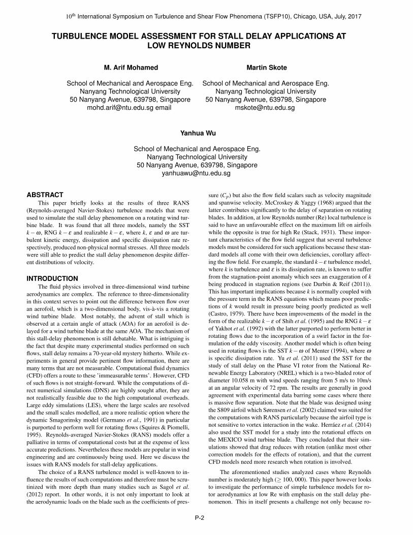
where P∞ and Pstatic are ambient pressure (taken far upstream onthe rotating blade) and static pressure respectively. Urotor, r andΩ represent the velocity at the rotor plane, local blade radius andangular velocity. The Cp distribution on the suction side of the bladeat different blade instances are depicted in Figure 2. As shown inFigure 2a , all three turbulence models were able to predict stall-delay albeit not matching the exact values of the experiments. At0.25R, the SST predicted two peaks which suggests the possibilityof a separation bubble in the region 0.05 ≤ x/c ≤ 0.16. The profiles

(a) Computational domain of the calculations. The top, bottom and thesides of the computational domain were set as inlet.

(b) A cut plane of the mesh depicting ten prismatic layers grown normalto the blade wall.

Figure 1: Computational domain and mesh of the model.

for Cp for the three turbulence models remain almost unchanged at0.55R and 0.75R. The realizable and RNG k−ε continued to show ahigh lift component near the leading edge while the SST displayed anotably low peak very close to the leading edge at 0.55R and 0.75R.Interestingly enough, the RNG showed a good match of Cp with theexperiments at 0.55R.

The Reynolds stresses, uiu j in two-equation models are notcomputed explicitly as they are in second moment closure modelsand as such they are modelled. The formulation for Reynolds stressin two-equation models is uiu j = −2νtSi j +

23 kδi j where Si j is the

strain rate tensor.One of the issues with this formulation is the possibility of neg-

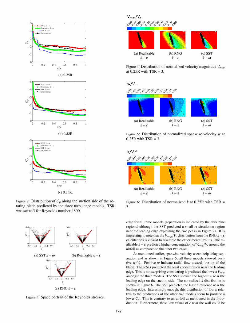
ative normal stresses which is permissible if the first term on the lefthand side eclipses the second term. Negative normal stresses arenon-physical and violates the Cauchy-Schwartz inequality. A goodway to show realistic, hence realizable, normal stresses is look atthe phase-space portrait or the Lumley triangle. All non-realizablenormal stresses occupy the space outside of the triangle. A vir-tual spherical volume was wrapped around the blade and hub andReynolds stresses were extracted in this volume. Figure 3 showsthe behaviour of the normal stresses via the Lumley triangle thatare computed by the k−ω , RNG k− ε SST k−ω and realizablek − ε turbulence models for the rotating case. It is immediatelyobvious that there is a substantial degree of non-realizable stressescomputed by all models, surprisingly even in the realizable k− ε .

The contours of relative velocity magnitude normalized by therelative velocity Vr, defined as the modulus of the term in parenthe-sis of Equation (1), for all three models taken at the 0.25R planeare shown in Figure 4. As the emphasis of this study is on stalldelay which occurs at the inboard, only the contours at 0.25R areshown. As seen, there is no indication of separation near the leading

P-2

x/c0 0.2 0.4 0.6 0.8 1

Cp

-5

-4

-3

-2

-1

0

RNG k − ǫ

Realizable k − ǫ

SST k − ω

Experiments

(a) 0.25R

x/c0 0.2 0.4 0.6 0.8 1

Cp

-5

-4

-3

-2

-1

0

RNG k − ǫ

Realizable k − ǫ

SST k − ω

Experiments

(b) 0.55R

x/c0 0.2 0.4 0.6 0.8 1

Cp

-5

-4

-3

-2

-1

0

RNG k − ǫ

Realizable k − ǫ

SST k − ω

Experiments

(c) 0.75R.

Figure 2: Distribution of Cp along the suction side of the ro-tating blade predicted by the three turbulence models. TSRwas set at 3 for Reynolds number 4800.

ζ-0.4 -0.2 0 0.2 0.4

η

0

0.2

0.4

(a) SST k−ω

ζ-0.4 -0.2 0 0.2 0.4

η

0

0.2

0.4

(b) Realizable k− ε

ζ-0.4 -0.2 0 0.2 0.4

η

0

0.2

0.4

(c) RNG k− ε

Figure 3: Space portrait of the Reynolds stresses.

(a) Realizablek− ε

(b) RNGk− ε

(c) SSTk−ω

Figure 4: Distribution of normalized velocity magnitude Vmagat 0.25R with TSR = 3.

(a) Realizablek− ε

(b) RNGk− ε

(c) SSTk−ω

Figure 5: Distribution of normalized spanwise velocity w at0.25R with TSR = 3.

(a) Realizablek− ε

(b) RNGk− ε

(c) SSTk−ω

Figure 6: Distribution of normalized k at 0.25R with TSR =3.

edge for all three models (separation is indicated by the dark blueregions) although the SST predicted a small re-circulation regionnear the leading edge explaining the two peaks in Figure 2a. It isinteresting to note that the Vmag/Vr distribution from the RNG k−ε

calculations is closest to resemble the experimental results. The re-alizable k−ε predicted higher concentration of Vmag/Vr around theairfoil as compared to the other two cases.

As mentioned earlier, spanwise velocity w can help delay sep-aration and as shown in Figure 5, all three models showed posi-tive w/Vr. Positive w indicate radial flow towards the tip of theblade. The RNG predicted the least concentration near the leadingedge. This is not surprising considering it predicted the lowest Vmagamongst the three models. The SST showed the highest w near theleading edge on the suction side. The normalized k distribution isshown in Figure 6. The SST predicted the least turbulence near theleading edge. Interestingly enough, this distribution of low k rela-tive to the predictions of the other two models seem to produce alower Cp. This is contrary to an airfoil as mentioned in the Intro-duction. Furthermore, these low values of k near the wall could be

P-2

due to the fact that the SST does not incorporate a wall functionunlike the other two models, and also because of the cross diffusionterm in the SST which dampens turbulence.

CONCLUSIONSThree turbulence models namely the RNG k − ε , Realizable

k− ε and the SST k−ω were used to simulate the stall-delay phe-nomenon on the S805 wind turbine blade. It should be promul-gated that none of these models should be used when investigatingReynolds stresses due to non-realizable behavior shown by all mod-els (even the realizable k− ε). The results also show vast differentbehaviors of velocity between the three models even though the allthree models predicted the delay of stall via the surface pressuredistributions on the blade.

REFERENCESCastro, IP 1979 Numerical difficulties in the calculation of com-

plex turbulent flows. In Turbulent Shear Flows I, pp. 220–236.Springer.

Durbin, Paul A & Reif, BA Pettersson 2011 Statistical theory andmodeling for turbulent flows. John Wiley & Sons.

Germano, Massimo, Piomelli, Ugo, Moin, Parviz & Cabot,William H 1991 A dynamic subgrid-scale eddy viscosity model.Physics of Fluids A: Fluid Dynamics (1989-1993) 3 (7), 1760–1765.

Herraez, Ivan, Stoevesandt, Bernhard & Peinke, Joachim 2014 In-sight into rotational effects on a wind turbine blade using navier–stokes computations. Energies 7 (10), 6798–6822.

Lee, Hsiao Mun & Wu, Yanhua 2015 A tomo-piv study of the ef-fects of freestream turbulence on stall delay of the blade of ahorizontal-axis wind turbine. Wind Energy 18 (7), 1185–1205.

McCroskey, WJ & Yaggy, PF 1968 Laminar boundary layers on

McCroskey, WJ & Yaggy, PF 1968 Laminar boundary layers onhelicopter rotors in forward flight. AIAA journal 6 (10), 1919–1926.

Menter, Florian R 1994 Two-equation eddy-viscosity turbulencemodels for engineering applications. AIAA journal 32 (8), 1598–1605.

Rumsey, Christopher L & Spalart, Philippe R 2009 Turbulencemodel behavior in low reynolds number regions of aerodynamicflowfields. AIAA journal 47 (4), 982–993.

Sagol, Ece, Reggio, Marcelo & Ilinca, Adrian 2012 Assessmentof two-equation turbulence models and validation of the perfor-mance characteristics of an experimental wind turbine by cfd.ISRN Mechanical Engineering 2012.

Shih, Tsan-Hsing, Liou, William W, Shabbir, Aamir, Yang, Zhigang& Zhu, Jiang 1995 A new k-ε eddy viscosity model for highreynolds number turbulent flows. Computers & Fluids 24 (3),227–238.

Sørensen, Niels N, Michelsen, JA & Schreck, S 2002 Navier–stokespredictions of the nrel phase vi rotor in the nasa ames 80 ft× 120ft wind tunnel. Wind Energy 5 (2-3), 151–169.

Squires, Kyle D & Piomelli, Ugo 1995 Dynamic modeling of rotat-ing turbulence. In Turbulent Shear Flows 9, pp. 71–83. Springer.

Stack, John 1931 Tests in the variable density wind tunnel to inves-tigate the effects of scale and turbulence on airfoil characteristics.

Yakhot, VSASTBCG, Orszag, SA, Thangam, S, Gatski, TB &Speziale, CG 1992 Development of turbulence models for shearflows by a double expansion technique. Physics of Fluids A:Fluid Dynamics (1989-1993) 4 (7), 1510–1520.

Yu, Guohua, Shen, Xin, Zhu, Xiaocheng & Du, Zhaohui 2011 Aninsight into the separate flow and stall delay for hawt. RenewableEnergy 36 (1), 69–76.

P-2