26
Turbulens – Teori och modellering

Turbulens – Teori ochmodellering

Introduction
Two questions:
• Why did you chose this course?
• What are your expectations?

Turbulence – Theory and modelling
•Understanding the phenomena that affects the
transition from laminar to turbulent flow
•Knowledge about the theory for describing turbulent
flow
•Knowledge about turbulence models applicability
and limitations
•Ability to analyse a flow situation and chose a
propper modelling approach accordingly
Goals

Turbulence – Theory and modelling
•Be able to describe the physical mechanisms of the transition from
laminar to turbulent flow for a simple flow case
•Be able to explain Kolmogorov’s theory, including the basic
assumptions and the validity of the theory
•Be able to, from a phenomenological perspective, assess if a flow is
turbulent
•Be able to explain some of the important and basic terms of the subject
•Be able to describe the character of the turbulence in different flow
situations with respect to the properties and development of the
turbulence, and explain how the differences between these flow
situations are reflected in the modelling
Goals

Turbulence – Theory and modelling
•Be able to analyse a flow case and suggest a method for numerical
simulation with respect to governing equations, possible simplifications
and choice of turbulence model, and also to compare with alternative
methods.
•Be able to scrutinise and from given criteria estimate the credibility of
results from turbulent flow simulations
•Be able to actively participate in discussion of problems relevant for
the subject
•Be able to present, both orally and in writing, a technical report
containing analyses and choice of turbulence model
Goals (continued)

Turbulence – Theory and modelling
•To pass (grade 3) the following is required:
• Approved home works, lab-report and group study (GS)
• Participation in the computer exercises
•Oral exam for higher grade (grades 4 and 5)
•Participation in the laboratory exercise, computer exercises and the
guest lecture is mandatory.
•The home works are handed in individially. However, you are alowed,
even encouraged, to work in groups discussing the problems.
•The groups study is to be presented both in writing as well as orally.
One report per group.
Examination and requirements


Turbulence

Two questions
1. How would you describe turbulence? Think about key-words to characterise it.
2. Think about situations where turbulent flow is better than laminar and vice versa.

Turbulence
• Random
• 3D
• Diffusive
• Dissipative
• Property of the flow
• High Reynolds number
• Continuum

Turbulence
Big whirls have little whirls
Which feed on their velocity
Little whirls have lesser whirls
And so on to viscosity – in the
molecular sense
L F Richardson
Turbulence
I am an old man now, and when I die
and go to Heaven there are two matters
on which I hope enlightenment. One is
quantum electro-dynamics and the
other is turbulence of fluids. About the
former, I am really rather optimistic.
Sir Horace Lamb

outflow
Heating/Cooling
Impingement wall
nozzleMean Sherwood number Sherwood number fluctuation

0i
i
x
u
i
j
ij
j
i
jij
jiiF
xx
u
xx
p
x
uu
t
u
1
Models for
turbulence,
combustion etc.
Geometry
Mathematical
description Results
For example velocity, pressure,
temperature
Numerical
methods

Question
• Why do we need to model turbulence?

Turbulence modelling
Example:
Pipe flow, turbulent Reynolds number, Re = 10000
Relation between largest and smallest scales ~ Re3/4
No. of nodes ~ Re9/4 2109 ca. 30 gigabyte RAM
Conclusion: Model needed

Turbulence modelling
Isotropic turbulence in a box
Turbulence modelling
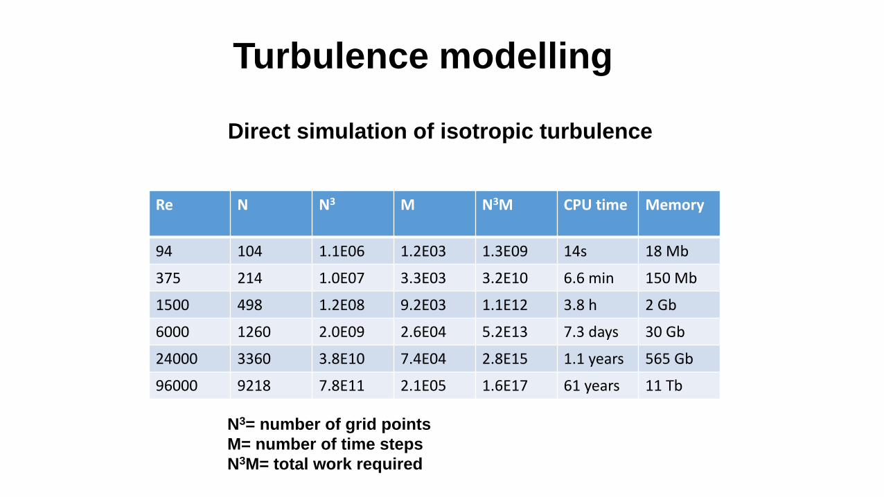
Direct simulation of isotropic turbulence
Required time at a computing rate of 82 Gflop
Re N N3 M N3M CPU time Memory
94 104 1.1E06 1.2E03 1.3E09 14s 18 Mb
375 214 1.0E07 3.3E03 3.2E10 6.6 min 150 Mb
1500 498 1.2E08 9.2E03 1.1E12 3.8 h 2 Gb
6000 1260 2.0E09 2.6E04 5.2E13 7.3 days 30 Gb
24000 3360 3.8E10 7.4E04 2.8E15 1.1 years 565 Gb
96000 9218 7.8E11 2.1E05 1.6E17 61 years 11 Tb
N3= number of grid points
M= number of time steps
N3M= total work required

Turbulence
Instantaneous velocity field of a round jet
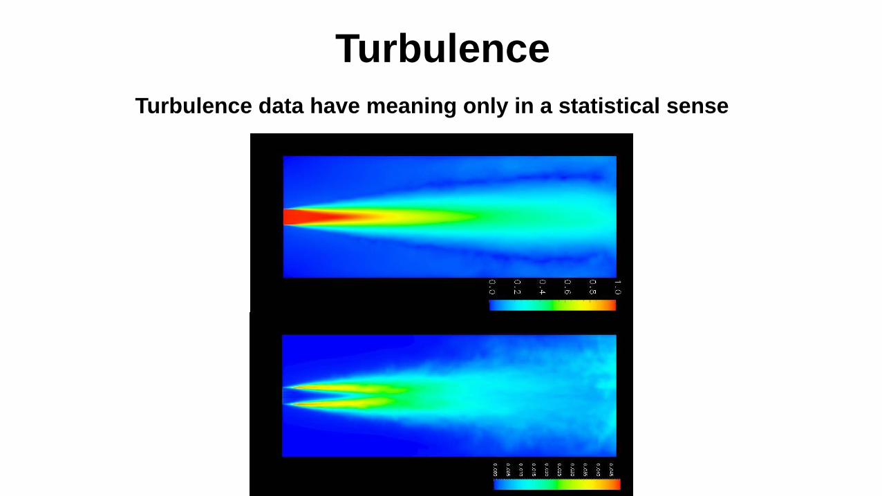
Turbulence
Mean velocity
Turbulent
kinetic energy
Turbulence data have meaning only in a statistical sense
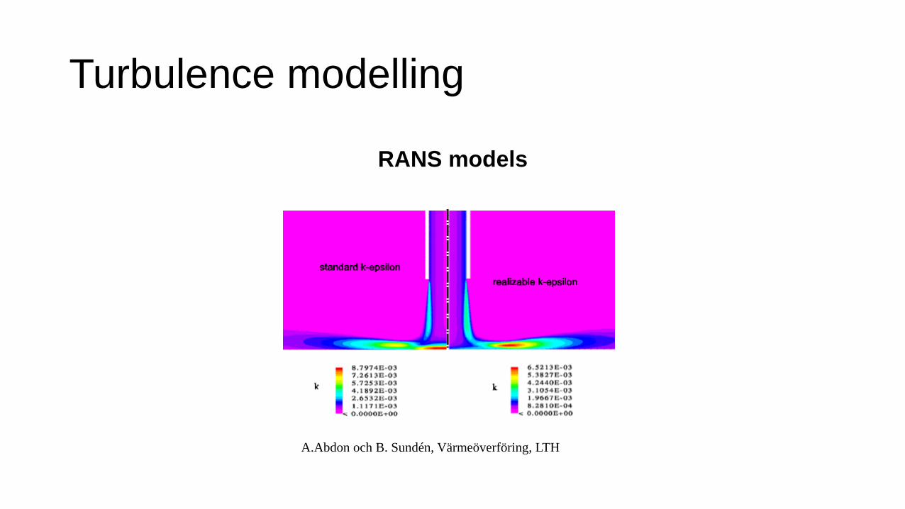
Turbulence modelling
RANS models
A.Abdon och B. Sundén, Värmeöverföring, LTH
Turbulence
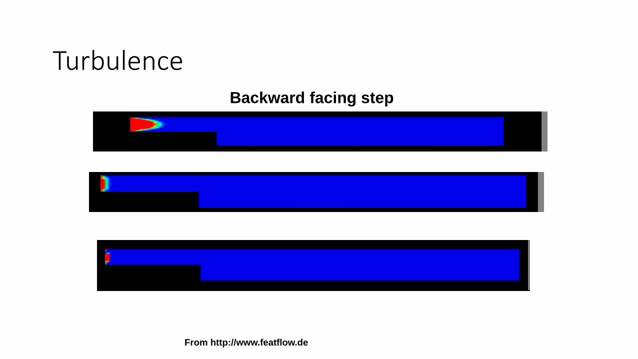
From http://www.featflow.de
Backward facing step

Discussion:
Are these flows laminar or
turbulent? Motivate.

Turbulence
Brief history:• 15th century, da Vinci, observations of turbulence
• 18th century, Euler, equations for inviscid flow
• Early 19th century, Navier and Stokes, the N-S equations
• 1883, Reynolds, flow instability in pipe flow
• 1904, Prandtl, boundary layer theory
• 1941, Kolmogorov, theory on turbulent scales
• 1963, Smagorinsky, first sub-grid scale model for LES
• 1970, Launder et al., two-equation model for turbulence

Turbulence
Leonardo da Vinci

Turbulence
Laminar
Turbulent
Osborne Reynolds (1883)
ULReReynolds number:


