OPEN ACCESS Turbulent cascades, transfer, and scale interactions in magnetohydrodynamics To cite this article: A Alexakis et al 2007 New J. Phys. 9 298 View the article online for updates and enhancements. You may also like Local and nonlocal advected invariants and helicities in magnetohydrodynamics and gas dynamics I: Lie dragging approach G M Webb, B Dasgupta, J F McKenzie et al. - Nonlinear motion of non–uniform current–vortex sheets in MHD Richtmyer–Meshkov instability Chihiro Matsuoka - Subgrid-scale modeling for the study of compressible magnetohydrodynamic turbulence in space plasmas A A Chernyshov, K V Karelsky and A S Petrosyan - This content was downloaded from IP address 92.202.63.64 on 16/03/2022 at 09:57
Transcript
OPEN ACCESS
Turbulent cascades, transfer, and scaleinteractions in magnetohydrodynamicsTo cite this article: A Alexakis et al 2007 New J. Phys. 9 298
View the article online for updates and enhancements.
You may also likeLocal and nonlocal advected invariantsand helicities in magnetohydrodynamicsand gas dynamics I: Lie draggingapproachG M Webb, B Dasgupta, J F McKenzie etal.
-
Nonlinear motion of non–uniformcurrent–vortex sheets in MHDRichtmyer–Meshkov instabilityChihiro Matsuoka
-
Subgrid-scale modeling for the study ofcompressible magnetohydrodynamicturbulence in space plasmasA A Chernyshov, K V Karelsky and A SPetrosyan
-
This content was downloaded from IP address 92.202.63.64 on 16/03/2022 at 09:57
T h e o p e n – a c c e s s j o u r n a l f o r p h y s i c s
New Journal of Physics
Turbulent cascades, transfer, and scale interactionsin magnetohydrodynamics
A Alexakis1,2, P D Mininni1,3 and A Pouquet1
1 National Center for Atmospheric Research, P O Box 3000, Boulder,CO 80307, USA2 Laboratoire Cassiopee, Observatoire de la Cote d’Azur, BP 4229,Nice Cedex 04, FranceE-mail: [email protected], [email protected] and [email protected]
New Journal of Physics 9 (2007) 298Received 7 January 2007Published 31 August 2007Online at http://www.njp.org/doi:10.1088/1367-2630/9/8/298
Abstract. The nature of the interactions between different scales in magneto-hydrodynamic (MHD) turbulence is important for the understanding of thebehaviour of magnetized astrophysical, geophysical and industrial flows in aturbulent state. In this paper, we review some recent results in the study of localityof interactions in turbulent flows and we address some of the questions that arise.We examine the cascade of ideal invariants in turbulent MHD flows by examiningthe transfer functions. We show new results indicating that the nonlocal behaviourof the energy transfer in MHD is the result of a correlation between the velocityand magnetic fields. This nonlocality disappears if we randomize the phases of thetwo fields keeping the hydrodynamic and magnetic helicities fixed. The cascadeof magnetic helicity is also investigated, with special focus on the fate of thesmall-scale helicity and its coupling with the large-scale flow. These results haveimplications for dynamo action, in particular for the commonly used distinctionbetween large- and small-scale dynamos. The long-range interactions that existin MHD flows also raise the question of the existence of universality in MHD,both in the kinematic dynamo regime as well as in the turbulent steady state.
3 Author to whom any correspondence should be addressed.
1. Introduction 22. Energy transfer and structures in MHD turbulence 43. Magnetic helicity cascade 94. Large- and small-scale dynamos 135. Conclusions 16Acknowledgments 17References 17
1. Introduction
Most of the barionic matter in the universe is in an ionized turbulent state coupled to magneticfields strong enough to play a dynamical role in the involved processes; e.g. in solar and stellarwinds, in accretion disks, and in the interstellar medium. Although in many cases a completedescription requires a generalized Ohm’s law and the inclusion of kinetic plasma effects [1]–[3], in general the large scales can be properly described by the magnetohydrodynamic (MHD)approximation [4]. Moreover, the Reynolds numbers (the ratio of nonlinear to dissipation terms)in these systems are large and the flows are in a turbulent state. It is essential therefore tounderstand and quantify the statistical properties of MHD turbulence in order to understand andpredict the physical evolution of many astrophysical and geophysical systems.
In the Kolmogorov description of hydrodynamic turbulence, the interactions of similarsize eddies play the basic role of cascading the injected energy to smaller scales on a timescaleτl = l/ul, where l is the examined length scale and ul the characteristic velocity at this scale. Thisprocedure persists up to the dissipation length scale where energy is finally dissipated. Imposinga constant energy flux ε = u2
l /τl at the inertial range leads to the well verified (up to intermittencycorrections) scaling u2
l ∼ l2/3, or in spectral space E(k) ∼ k−5/3. The role of the large-scale flowin this scenario is limited to just advecting the small size eddies without significantly distortingthem. One then expects that the resulting structures in scales sufficiently small are independentof the way the system is forced in the large scales and have therefore a universal behaviour.
It has been shown however even for simple hydrodynamic flows in both experiments [5]–[8]and numerical simulations [9, 10] that the large-scale flow still plays an important role in thecascade of energy and the formation of structures in the small scales. In numerical simulationswith Reynolds numbers as high as Rλ ∼ 800, it was observed that 20% of the energy flux inthe small scales is due to interactions with the large-scale flow. This represents a deviation fromself-similarity, and the presence of nonlocal interactions can be associated with clustering ofvortex tubes in regions of intense large-scale shear [10], the presence of long-time correlationsin the small scales (compared with the eddy turnover time) [8], slower than expected recovery ofisotropy [11], and intermittency [12] (which in turn implies corrections to the energy spectrum).Here, Rλ = Uλ/ν denotes the Reynolds number based on the Taylor lengthscale, defined in thesimulations as λ = 2π(
∫E(k)dk/
∫E(k)k2dk)1/2 (2π is the size of the computational domain),
U = 〈u2〉1/2 is the r.m.s. velocity, and ν the kinematic viscosity of the fluid.In MHD flows, the role of the large-scale flow and large-scale magnetic structures is expected
to be even more important since the effect of a large-scale magnetic field cannot be ‘taken away’
New Journal of Physics 9 (2007) 298 (http://www.njp.org/)
by a Galilean transformation as the velocity in both the hydrodynamic and MHD case. As aresult, small scales can interact directly with the large scales and we cannot a priori followthe same arguments Kolmogorov used in hydrodynamic turbulence. So assumptions of localityof interactions are in question. Accordingly, some phenomenological models try to take intoaccount the effect of nonlocal interactions assuming a small size eddy interacts strongly withthe large-scale magnetic field and the energy cascades on a longer timescale τl ∼ B0l/u
2l , where
B0 is the characteristic amplitude of the magnetic field at the large scales. Assuming a constantflux ε ∼ u2
l /τl leads to the Iroshnikov–Kraichnan scaling u2l ∼ l1/2 that results in the k−3/2 power
law for the energy spectrum [13, 14]. Similar phenomenological models that take into accountthe anisotropy due to the large-scale magnetic field have also been investigated in the literature[15]–[19]. However, although these phenomenological descriptions assume that a large-scalefield has the effect of reducing the energy cascade rate, the transfer of energy (and the cascade)still takes place between eddies of similar size, an assumption that needs to be tested.
Before proceeding any further we need to clarify what we mean by local and nonlocalinteractions, local and nonlocal transfer, and local and nonlocal cascade of an ideal quadraticinvariant. Because of the quadratic form of the nonlinear terms in the incompressiblehydrodynamic and MHD equations, three wavenumbers are involved in any basic interaction,with the ideal invariant being transferred between two of the wavenumbers (say k and q) whilethe third wavenumber (say p) is responsible for the transfer [20, 21]. Because of the conditionk + q + p = 0, at least two of the wavenumbers have to be of the same order, while the third caneither be of the same order or much smaller than the other two. The interactions for which allthree wavenumbers are of the same order are going to be called local, and nonlocal, if otherwise.If the two wavenumbers that exchange energy (k and q) are of the same order we will talk aboutlocal transfer, and nonlocal, if otherwise. Note that locality of interactions implies locality oftransfer, but not the other way round. Finally, if in a given flow all interactions are present (bothlocal and nonlocal), we will talk about a local cascade when most of the flux of the invariant isdue to local interactions.
‘Kolmogorov-like’ phenomenological descriptions assume that most of the energy flux isdue to local interactions. There are two possible deviations from this local cascade: (i) the transferof an ideal invariant can be local (|k| ∼ |q|) but due to nonlocal interactions (|p| � |k| ∼ |q|),or (ii) the transfer itself can be nonlocal. In the results that we discuss in the following sectionsboth forms of nonlocality are present, but we will focus on the study of the nonlocal transfer.Also, in many of the examined cases both local and nonlocal transfers give contributions to thefluxes. We will refer to both processes as ‘cascades’ as long as the total flux of the invariant isconstant in a range of wavenumbers, to avoid introducing new terminology each time nonlocaltransfers appear.
With these definitions in mind we recall some of the recently obtained results in MHDturbulence. Authors [21]–[23] have shown that the locality of energy transfer is in questionin MHD flows. In particular, it was demonstrated from simulations that the transfer of energyin MHD has two components: a local one that shares similar properties with hydrodynamicturbulence, and a nonlocal component for which energy from the large scales is injecteddirectly into the small scales without the intervention of the intermediate scales. In dynamosimulations, during the kinematic stage of exponential amplification of magnetic energy (inwhich the magnetic field is too weak to feedback and modify the flow through the Lorenzforce and it is advected and stretched passively) this nonlocal behaviour appears to be evenstronger [24, 25].
New Journal of Physics 9 (2007) 298 (http://www.njp.org/)
The nonlocal transfer appears to be even stronger when one investigates the cascade ofmagnetic helicity. Magnetic helicity is an ideal invariant in MHD that is known to cascadeinversely (to the large scales) [26]–[30] in a turbulent flow. The generation of large-scale magneticfields, for example in galaxies and other astrophysical bodies, is attributed to the inverse cascadeof magnetic helicity. Nonlocal transfer of helicity has been observed [30] due to the ‘alpha’effect[26, 31, 32], where magnetic energy and helicity are injected in the largest scale of the systemdirectly from the forced scale. Furthermore, nonlocal transfer of helicity has also been observedbetween the largest scale of the flow and the smallest, even dissipative, scales. This latter processremoves magnetic helicity from the large scales, and is attributed to reconnection events thatallow the large-scale magnetic field to ‘unwind’, destroying in that way large-scale magnetichelicity.
Nonlocality appears to be an essential ingredient for a phenomenological understandingand description of MHD turbulence. The following questions then arise: what are the physicalprocesses and structures that result in this nonlocal behaviour? What are the implications on theflow properties and for its modelling? Can we still pursue a unique universal theory that describesMHD turbulence?
In this paper, we review previous results and present a new analysis of the transfer ofenergy and magnetic helicity in MHD flows. Section 2 introduces the equations and notation,and discusses the transfer of energy in MHD. Evidence of a connection between correlations ofthe velocity and magnetic fields, and nonlocal transfer of energy is presented. Section 3 considersthe transfer of magnetic helicity. The flux of magnetic helicity in Fourier space in mechanicallyforced simulations is studied in detail, and the coexistence of direct and inverse transfers ofhelicity in different scales is shown. Section 4 considers the implications of these results fordynamo simulations. In particular, a classification of small- and large-scale dynamos based onthe transfer of energy is attempted. Finally, section 5 summarizes the results and discusses theimplications for the notion of universality in turbulent MHD flows.
2. Energy transfer and structures in MHD turbulence
In the following sections we are going to investigate the incompressible MHD equations withPrandtl number PM = 1 (expressing the ratio of kinematic viscosity ν to magnetic diffusivity η).Some cases with PM < 1 will be considered in section 4. The results that are going to be presentedare based on direct numerical simulations (DNS) of the MHD equations solved by a dealiasedpseudospectral method in triple periodic boxes. No uniform magnetic field is imposed in any ofthe simulations studied.
The equations that describe the dynamics of an incompressible conducting fluid coupled toa magnetic field in the MHD approximation are given by:
∂tu + u · ∇u = −∇p + b · ∇b + ν∇2u + f, (1)
∂tb + u · ∇b = b · ∇u + η∇2b, (2)
∇ · u = 0, ∇ · b = 0, (3)
where u is the velocity field, b is the magnetic field, and p is the (total) pressure. Here, f is theexternal force that drives the turbulence and the dynamo process that sustains magnetic fieldagainst Ohmic dissipation.
New Journal of Physics 9 (2007) 298 (http://www.njp.org/)
To investigate the transfer of energy among different scales in a turbulent flow we willintroduce the shell filter decomposition of the two fields:
u(x) =∑K
uK(x), b(x) =∑K
bK(x),
where
uK(x) =∑
K < |k| �K+1
u(k)eikx, and bK(x) =∑
K < |k| �K+1
b(k)eikx,
where u(k) and b(k) are the Fourier transforms of the two fields with wavenumber k. The fieldsuK and bK are therefore defined as the part of the velocity and magnetic field respectively, whoseFourier transform contains only wavenumbers in the shell (K, K + 1] (hereafter called the shellK). Alternatively, the shells can be defined in a logarithmic binning (γnK0, γ
n+1K0] for somepositive γ > 1 and integer n. However, logarithmic binning cannot distinguish transfer betweenlinearly neighbouring shells (K to K + 1) from the transfer between logarithmic neighbouringshells (K to γK). If in MHD the energy cascade is the result of interactions with the large-scalefield (e.g. at the forced scale k−1
f ), the energy in a shell K � kf will be transferred into the shellK + kf and logarithmic binning will not be able to distinguish this transfer from the transfer dueto local interactions. For this reason, we use linear binning but we note that care needs to be takenwhen using the word ‘scale’ that implies in general a logarithmic division of the wavenumbers.The transfer among logarithmic shells can be reconstructed at any time later by summing overthe linearly spaced shells.
The evolution of the kinetic energy in a shell K, Eu(K) = ∫u2
K/2 dx3 is given by:
∂tEu(K) =∑Q
[Tuu(Q, K) + Tbu(Q, K)] − νDu(K) + F(K), (4)
∂tEb(K) =∑Q
[Tbb(Q, K) + Tub(Q, K)] − ηDb(K). (5)
Here we have introduced the functions F(K), Du(K), Db(K) that express respectively the energyinjection and dissipation in the shell K, and the transfer functions Tuu(Q, K), Tub(Q, K),Tbb(Q, K), and Tbu(Q, K), that express the energy transfer between different fields and shells:
Tuu(Q, K) ≡ −∫
uK(u · ∇)uQ dx3, Tbu(Q, K) ≡∫
uK(b · ∇)bQ dx3, (6)
Tbb(Q, K) ≡ −∫
bK(u · ∇)bQ dx3, Tub(Q, K) ≡∫
bK(b · ∇)uQ dx3. (7)
The function Tuu(Q, K) expresses the transfer rate of kinetic energy lying in the shell Q tokinetic energy lying in the shell K, due to the advection term in the momentum equation (1).Similarly, Tbb(Q, K) expresses the rate of energy transfer of magnetic energy lying in the shellQ to magnetic energy lying in the shell K due to the magnetic advection term. The Lorentzforce is responsible for the transfer of energy from the magnetic field in shell Q to the velocity
New Journal of Physics 9 (2007) 298 (http://www.njp.org/)
field in the shell K, and the resulting transfer function is given by Tbu(Q, K). Finally, the termresponsible for the stretching of the magnetic field lines in the induction equation (2) results inthe transfer of kinetic energy to magnetic energy, and is expressed by Tub(Q, K). These transferfunctions satisfy
Tvw(Q, K) = −Twv(K, Q). (8)
(where v, w can be either u and/or b). This expression indicates that the rate at which the shellQ gives energy to the shell K is equal to the rate the shell K receives energy from the shell Q.
The shell-to-shell energy transfer functions have been studied extensively for a variety ofmechanically forced and decaying MHD flows in two and three dimensions, in the saturatedturbulent regime and in the kinematic dynamo regime [20]–[22], [25, 33, 34]. Here we presenta short summary of the results. In all cases examined in the literature the transfers Tuu andTbb have a local behaviour: energy is transferred forward between nearby shells, from slightlysmaller wavenumbers to slightly larger wavenumbers. This is similar to what is measured inhydrodynamic turbulence [9, 10], [35]–[38]. On the other hand, the transfers Tbu and Tub, thatexpress the energy exchange between the two different fields, have a rather different behaviour.The magnetic field in a shell K receives energy at the same rate from all wavenumbers smallerthan K, and gives energy to shells with slightly larger wavenumbers. In addition, when the systemis mechanically forced there is a strong input of magnetic energy directly from the forced scaleto all shells [21, 23, 34]. This kind of transfer is absent in free decaying runs [22]. We note thatin mechanically forced runs, the velocity field has to supply energy to the magnetic field all thetime in order to sustain the magnetic field against Ohmic dissipation. This is not necessarily truefor freely decaying runs where both fields are dissipated in time. As a result, some differencescan be expected in the transfer function of mechanically forced dynamos, free decaying runs,and electrically forced flows (not examined here).
A natural question to ask is: why the transfer between two different fields (expressed by thefunctions Tbu and Tub) is so different than the transfers among the same field (Tuu and Tbb)? Theanswer we will support in the present paper is that correlations between the velocity field andmagnetic field make shells of widely separated wavenumbers efficient for the transfer of energy.To support this claim we compare the energy transfer of two different sets of velocity and magneticfields (u, b). The first set (u1, b1) comes from a (numerical) solution of the MHD equations: aturbulent MHD flow resulting from a saturated dynamo simulation with ABC (helical) forcingacting at the wavenumber kf ≈ 3. The Reynolds numbers of the flow are Re = Rm ≈ 820 withRe = UL/ν and Rm = UL/η the mechanical and magnetic Reynolds numbers respectively,based on the integral scale of the flow L = 2π(
∫E(k)k−1dk/
∫E(k)dk). The simulation was
done on a 2563 grid. The second set of fields (u2, b2) was created by taking the first set andrandomizing the phases of each Fourier coefficient under the procedure u2(k) = eiφk u1(k) andb2(k) = eiψk b1(k), where φk and ψk are random numbers that depend only on the wavenumberk. In this way, incompressibility of each field, the kinetic and magnetic energy spectra, and thekinetic and magnetic helicities remain unchanged. However, the cross helicity of the two fieldscan change, which is a desired effect since we want to destroy correlations between the fieldsand their modes. In practice, five different realizations were used for the fields (u2, b2). Eachrealization was obtained by applying a different sequence of random phases to the fields (u1, b1).The transfers resulting from each realization were averaged at the end.
A cross-section of the z-component of the current density (jz, with j = ∇ × b) for the twosets is shown in figure 1. The thin filaments with strong current that appear in the right panel
New Journal of Physics 9 (2007) 298 (http://www.njp.org/)
Figure 1. Cross-section showing the z-component of the current density on thex–y plane in the MHD simulation (left) and in the set after randomizing phasesin Fourier space (right). Note that thin filaments in the cross-section, associatedwith current sheets in the 3D flow, have disappeared in the right panel.
Figure 2. Probability density function of the z-component of the current densityfor the magnetic field b1 from the numerical simulation (left panel), and for themagnetic field b2 after randomizing phases (right panel).
(resulting from the numerical solution of the MHD equations) are associated with cross-sectionsof current sheets in the three-dimensional (3D) box. The right panel shows the same cross-sectionfor the randomized magnetic field. In this case the thin filaments have disappeared. Figure 2 showsthe probability density function of jz for the two sets. The stretched exponential distribution withstrong tails denoting intermittency that results from the magnetic field b1 stemming from thenumerical simulation (left panel), transforms into a Gaussian distribution for the randomizedfield b2 (right panel).
Using these two sets the transfer functions were calculated. Figure 3 shows Tuu(Q, K) andTub(Q, K) for a fixed value of K = 25. The solid line shows the transfer functions for the solutionof the MHD equations (u1, b1), and the dashed line shows the same transfers for the randomphased fields (u2, b2). Although the transfers for the random phased fields are noisier, the shape
New Journal of Physics 9 (2007) 298 (http://www.njp.org/)
Figure 3. Transfer functions Tuu (left panel) and Tub (right panel) at a fixedvalue of K = 25 for the velocity and magnetic field stemming from a numericalsimulation (u1, b1) (solid lines) and for the set with randomized phases (u2, b2)
(dashed lines).
of the Tuu transfer is similar to the (u1, b1) set: most of the transfer results from nearby shells.This is expressed in the solid and dashed lines in the left panel of figure 3 by the positive peakto the left of Q = K = 25, and by the negative peak to the right of Q = K = 25 in Tuu(Q, K).The negative peak in Tuu expresses kinetic energy is taken from wavenumbers Q slightly smallerthan K = 25, while the positive peak denotes kinetic energy is given to wavenumbers Q slightlylarger than K = 25. The transfer of kinetic energy due to the advection term in the momentumequation (1) is as a result local and direct, for both sets (u1, b1) and (u2, b2). The fact that theamplitude of the transfer functions is smaller for (u2, b2) probably reflects that the fields withrandomized phases being less intermittent, third order quantities in the fields (as the energy fluxand transfers) are smaller.
The transfer Tub behaves differently. For (u1, b1), Tub peaks at Q ≈ 3, where mechanicalenergy is injected by the external forcing, and it is positive for all wavenumbers 0 < Q < K = 25(the ‘plateau’). This expresses the result previously discussed. In mechanically forced MHDflows, kinetic energy is transferred directly from the forced scale and all shells with wavenumbersQ < K to magnetic energy at each shell K. The negative peak in Tub for Q > K = 25 indicatesmagnetic energy is transferred to kinetic energy at slightly larger wavenumbers. The functionTub(Q, K) is highly nonlocal for the set (u1, b1). However, for the set (u2, b2) the transfer ofenergy from the forced wavenumber Q ≈ 3 to the examined shell K = 25 disappears, as wellas the plateau. Most of the transfer is local but not clearly forward.
The difference in the transfer of the two fields can also be seen in figure 4 where a shadow-graph plot of Tub is shown. The nonlocal input of energy from the forced large-scale to themagnetic field at all scales, indicated by the horizontal red-green line (left panel) is absent in thecase with randomized phases (right panel). Off-diagonal transfers also disappear in the (u2, b2)
set, and for this set most of the Tbu transfer is concentrated close to the diagonal in the (Q, K)
plane. Note this transfer function does not have to be antisymmetric with respect to K and Q
(see equation (8)).We conclude that phase correlations for each field as well as correlations between the two
fields (velocity and magnetic fields) are important for the transfer, and a simple estimate ofthe amplitude of the velocity and magnetic field at different scales (i.e. as used in Kolmogorovphenomenology) is not sufficient to estimate the magnitude of the nonlinear terms. We note that
New Journal of Physics 9 (2007) 298 (http://www.njp.org/)
Figure 4. Transfer function Tub(Q, K) (from kinetic energy in the shell Q tomagnetic energy in the shell K) for the velocity and magnetic field stemmingfrom a DNS (u1, b1) (left panel) and for the set with randomized phases (u2, b2)
(right panel). The amplitude of both transfers was normalized to the maximumof |Tub(Q, K)|.
the correlation between velocity and magnetic fields is also known to be of importance for theenergy cascade when a strong guiding field is present [39].
3. Magnetic helicity cascade
Besides the evolution of the energy, the evolution of magnetic helicity can also play an importantrole in the dynamics of an MHD system. Early studies using mean-field theory [31, 32], discretescale models [40, 41], and turbulent closure models [26, 42] have shown within the frameworkof the approximations made that magnetic helicity cascades inversely from small scales to largescales. DNS [27]–[29], [43, 44] have verified the inverse transfer and/or cascade of magnetichelicity, as well as the generation of large-scale magnetic fields from small-scale helical forcing.To this inverse cascade of helicity are attributed the large-scale magnetic fields observed in manyastrophysical objects. Magnetic helicity is also observed in the solar photosphere in associationwith coronal mass ejections (CMEs) and sigmoids [45]–[49].
Typically, in numerical investigations of the inverse cascade of magnetic helicity, the flowis forced with a mechanical helical forcing at some intermediate scale, and after the systemhas reached a hydrodynamic turbulent steady state a small seed magnetic field is introduced(a ‘dynamo simulation’, as discussed in more detail in the next section). The stretching ofthe magnetic field lines by the helical flow amplifies the magnetic energy. The process alsocreates magnetic helicity of the same sign than the kinetic helicity in scales smaller thanthe forced scales, and magnetic helicity of the opposite sign in the larger scales. As themagnetic field grows stronger and the Lorentz force feeds back on to the flow, the magnetichelicity at the large scales cascades inversely to even larger scales until the largest scale of thesystem is reached. After this point the magnetic helicity and energy in the largest scale keepsgrowing possibly until magnetic diffusivity becomes important and saturates the growth [28].
New Journal of Physics 9 (2007) 298 (http://www.njp.org/)
The fate of the small-scale helicity has not been investigated as much. However, in largeReynolds number flows it is important to know if the small-scale magnetic helicity cascadesalso to larger scales (in which case it will pile up close to the forced scale or cancel some ofthe magnetic helicity of opposite sign in the large scales), or if it is transferred to smaller scaleswhere it can be destroyed by the magnetic diffusivity. In the former case, no net generation ofmagnetic helicity exists in the limit of infinite magnetic Reynolds number since both signs ofhelicity cancel. In the latter case, the small-scale helicity is dissipated even in the limit of infinitemagnetic Reynolds number, and the sign of the magnetic helicity in the large-scale prevails. Tofind the direction of the cascade of helicity one has to determine the sign of the helicity flux
�H(K) =∫
b <K · (u × b) dx3, (9)
where b<K is the magnetic field filtered so that only the wavenumbers in the range 0 < |k| < K
are kept (not to be confused with the band-pass filtered b field bK defined in the previous section).If the flux of helicity remains of the same sign for all wavenumbers the two signs of helicitycascade in opposite directions. If however both the small-scale positive helicity and the large-scale negative helicity cascade to large scales the flux of helicity will change sign close to theforcing scale.
A detailed examination of the cascading process of magnetic helicity in mechanically andelectrically forced flows was investigated in [30], where its transfer rate among different scaleswas measured from DNS. In the examined runs with mechanical forcing, a positive helical forcingwas applied at intermediate scales so that enough large scales were available for an inverse cascadeof magnetic helicity to develop. This election naturally limits the Reynolds numbers that can beresolved, and as a result only moderate Reynolds numbers were considered and scales smallerthan the forcing scale could not be considered as inertial range scales. In this work we re-examinethe same run (with forcing at kf ≈ 10 and a spatial resolution of 2563 grid points) along with arun forced with the same (positive) sign of kinetic helicity but at larger scales (kf ≈ 3 and thesame spatial resolution) to investigate the evolution of the magnetic helicity in the small scaleswith better scale separation. The corresponding Reynolds numbers are Re = Rm ≈ 240 in therun forced at kf ≈ 10, and Re = Rm ≈ 820 in the run forced at kf ≈ 3.
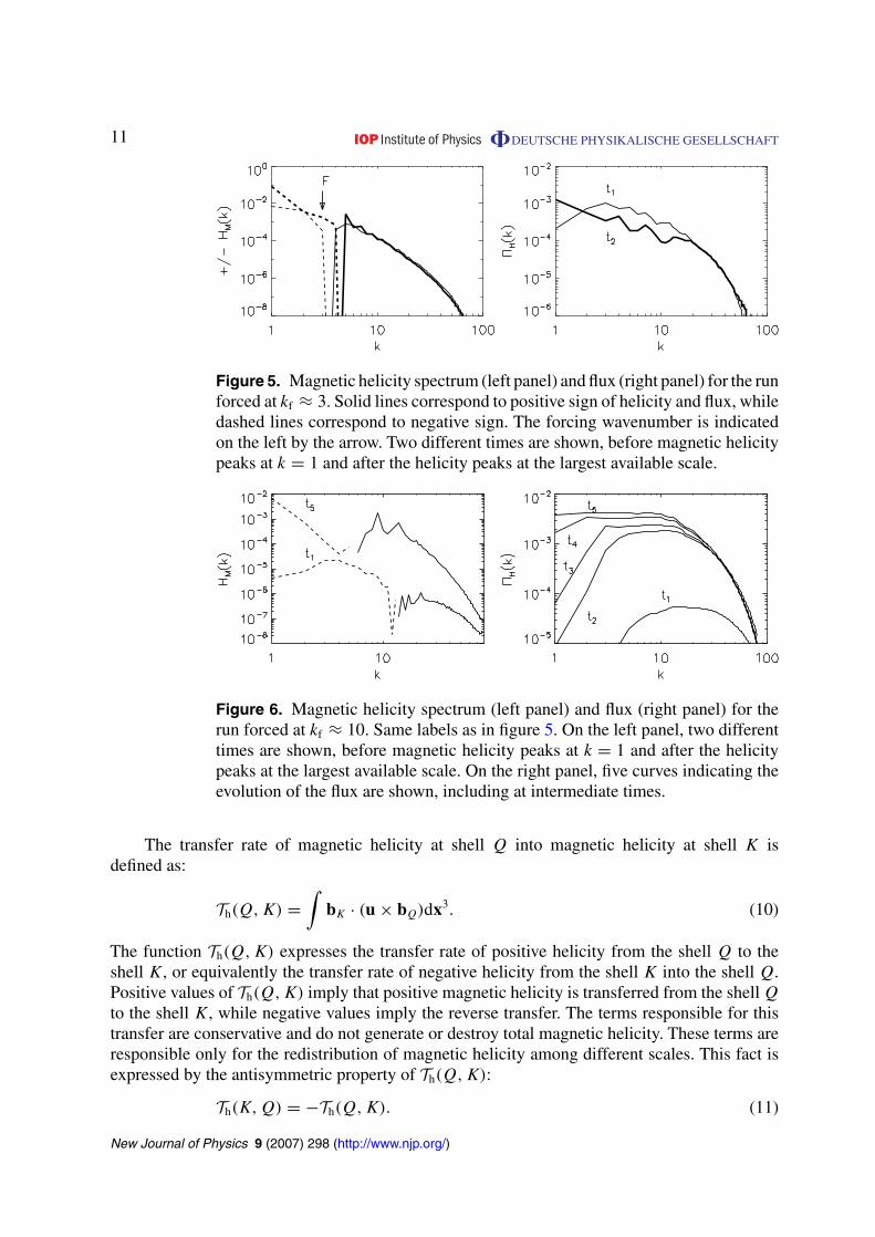
The magnetic helicity spectrum for the run forced at kf ≈ 3 is shown in figure 5 (leftpanel) along with the magnetic helicity flux (right panel) for several different times (the firsttime is before the magnetic helicity spectrum peaks at the largest scale, and the latter is after thespectrum peaks at the largest scale). For comparison we also show the magnetic helicity spectrumand flux for the run forced at kf ≈ 10 in figure 6. Clearly the flux remains of the same sign forall scales in both cases, even though the magnetic helicity changes sign at k ∼ kf . This impliesa different cascade direction for the two signs of magnetic helicity, i.e. that negative helicity(mostly concentrated at the large scales) cascades to larger scales, or equivalently that positivehelicity (mostly concentrated at scales smaller then the forcing scale) cascades to smaller scales.As a result, positive helicity cascading forward in scales smaller than the forcing scale, willdissipate when the dissipative scales are reached. At late times the negative magnetic helicity inthe large scales will dominate.
New Journal of Physics 9 (2007) 298 (http://www.njp.org/)
Figure 5. Magnetic helicity spectrum (left panel) and flux (right panel) for the runforced at kf ≈ 3. Solid lines correspond to positive sign of helicity and flux, whiledashed lines correspond to negative sign. The forcing wavenumber is indicatedon the left by the arrow. Two different times are shown, before magnetic helicitypeaks at k = 1 and after the helicity peaks at the largest available scale.
Figure 6. Magnetic helicity spectrum (left panel) and flux (right panel) for therun forced at kf ≈ 10. Same labels as in figure 5. On the left panel, two differenttimes are shown, before magnetic helicity peaks at k = 1 and after the helicitypeaks at the largest available scale. On the right panel, five curves indicating theevolution of the flux are shown, including at intermediate times.
The transfer rate of magnetic helicity at shell Q into magnetic helicity at shell K isdefined as:
Th(Q, K) =∫
bK · (u × bQ)dx3. (10)
The function Th(Q, K) expresses the transfer rate of positive helicity from the shell Q to theshell K, or equivalently the transfer rate of negative helicity from the shell K into the shell Q.Positive values of Th(Q, K) imply that positive magnetic helicity is transferred from the shell Q
to the shell K, while negative values imply the reverse transfer. The terms responsible for thistransfer are conservative and do not generate or destroy total magnetic helicity. These terms areresponsible only for the redistribution of magnetic helicity among different scales. This fact isexpressed by the antisymmetric property of Th(Q, K):
Th(K, Q) = −Th(Q, K). (11)
New Journal of Physics 9 (2007) 298 (http://www.njp.org/)
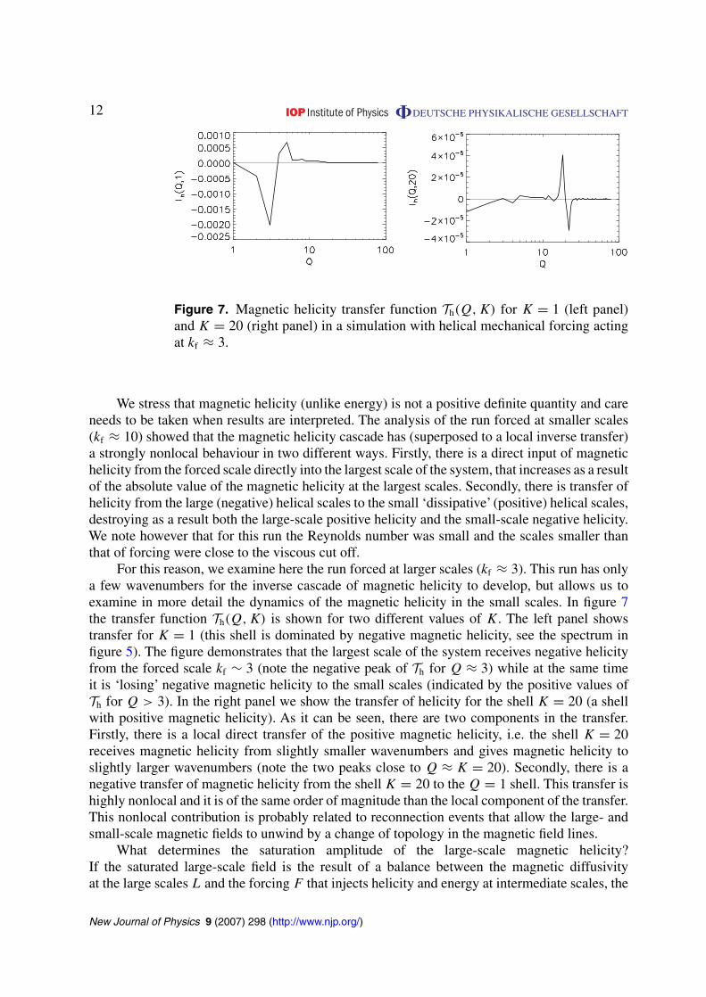
Figure 7. Magnetic helicity transfer function Th(Q, K) for K = 1 (left panel)and K = 20 (right panel) in a simulation with helical mechanical forcing actingat kf ≈ 3.
We stress that magnetic helicity (unlike energy) is not a positive definite quantity and careneeds to be taken when results are interpreted. The analysis of the run forced at smaller scales(kf ≈ 10) showed that the magnetic helicity cascade has (superposed to a local inverse transfer)a strongly nonlocal behaviour in two different ways. Firstly, there is a direct input of magnetichelicity from the forced scale directly into the largest scale of the system, that increases as a resultof the absolute value of the magnetic helicity at the largest scales. Secondly, there is transfer ofhelicity from the large (negative) helical scales to the small ‘dissipative’ (positive) helical scales,destroying as a result both the large-scale positive helicity and the small-scale negative helicity.We note however that for this run the Reynolds number was small and the scales smaller thanthat of forcing were close to the viscous cut off.
For this reason, we examine here the run forced at larger scales (kf ≈ 3). This run has onlya few wavenumbers for the inverse cascade of magnetic helicity to develop, but allows us toexamine in more detail the dynamics of the magnetic helicity in the small scales. In figure 7the transfer function Th(Q, K) is shown for two different values of K. The left panel showstransfer for K = 1 (this shell is dominated by negative magnetic helicity, see the spectrum infigure 5). The figure demonstrates that the largest scale of the system receives negative helicityfrom the forced scale kf ∼ 3 (note the negative peak of Th for Q ≈ 3) while at the same timeit is ‘losing’ negative magnetic helicity to the small scales (indicated by the positive values ofTh for Q > 3). In the right panel we show the transfer of helicity for the shell K = 20 (a shellwith positive magnetic helicity). As it can be seen, there are two components in the transfer.Firstly, there is a local direct transfer of the positive magnetic helicity, i.e. the shell K = 20receives magnetic helicity from slightly smaller wavenumbers and gives magnetic helicity toslightly larger wavenumbers (note the two peaks close to Q ≈ K = 20). Secondly, there is anegative transfer of magnetic helicity from the shell K = 20 to the Q = 1 shell. This transfer ishighly nonlocal and it is of the same order of magnitude than the local component of the transfer.This nonlocal contribution is probably related to reconnection events that allow the large- andsmall-scale magnetic fields to unwind by a change of topology in the magnetic field lines.
What determines the saturation amplitude of the large-scale magnetic helicity?If the saturated large-scale field is the result of a balance between the magnetic diffusivityat the large scales L and the forcing F that injects helicity and energy at intermediate scales, the
New Journal of Physics 9 (2007) 298 (http://www.njp.org/)
amplitude of the magnetic field at large-scale B0 should scale like B0 ∼ FL2/η which is verylarge. If however the non-local transfer of magnetic helicity is efficient enough to destroy large-scale helicity, saturation can be reached for smaller amplitudes of B0 (we note that in physicalsystems there is also expulsion of magnetic helicity from outflows that helps saturation of thelarge-scale magnetic field at smaller values). Of course an investigation of the saturation valueof the magnetic field in helical flows and its scaling with the magnetic Reynolds and magneticPrandtl numbers requires long (on the order of diffusive timescales) and high resolution runs,that are numerically too expensive to be investigated yet. It is likely however that the saturationamplitude of the large-scale magnetic field will depend on the way magnetic field lines reconnectin the small scales. It has been shown for example in [2] that the inclusion of the Hall effect(a term that acts on small scales) can increase substantially the saturation amplitude of themagnetic field in the large scales.
The observed direct transfer of magnetic helicity in scales smaller than the forcing scalehas also implications for estimations of the diffusion time of the small-scale magnetic helicity[50], and numerical and theoretical studies of the saturation of the α-effect in helical dynamos[28, 40, 41, 51]. Many models assume there is an inverse cascade of magnetic helicity at all scales,and as a result the small-scale magnetic helicity for very large magnetic Reynolds numbers shouldcancel part of the large-scale magnetic helicity. However when the small-scale magnetic helicityis transferred forward to small scales, it can be dissipated very fast (compared with the large-scale magnetic helicity). As a result, estimations of helicity production rates based on an inversetransfer at all scales should be revisited (see [30] for more details).
4. Large- and small-scale dynamos
The machinery to quantify transfer of ideal invariants between shells discussed in the previoussections can also be useful to determine what scales are involved in the amplification of themagnetic field during the kinematic stage of dynamos. Dynamos are often classified accordingto the scales in which magnetic energy is amplified: large- and small-scale dynamos, where largeand small is often defined relative to the energy containing scale of the turbulent hydrodynamicflow [51, 52]. Large-scale dynamos are often associated to helical flows, or to anisotropic andinhomogeneous flows (e.g. with a large-scale shear) [26]–[29], [44]. In large-scale dynamos (e.g.in mean field dynamos [31, 32]) the growth rate of the magnetic energy is in general a functionof the wavenumber. In the mean field dynamo description the generation of large-scale magneticfields (see e.g. [52]) in a turbulent flow requires the existence of small-scale fields, since thesources of magnetic energy in the large scales depend on the properties of the small-scale fieldsif the transfer of HM is nonlocal.
Small-scale dynamos, in which magnetic fields are correlated at scales smaller than theintegral scale of the flow, are often studied for magnetic Prandtl numbers PM > 1 as found inthe interstellar medium; nonhelical flows, and delta-correlated in time mechanical forcing aregenerally assumed [21, 53, 54]. Since when ν > η velocity fluctuations are damped fast in thesubviscous scales and the magnetic energy can grow during the kinematic dynamo regime inscales were velocity fluctuations are negligible, it is clear in this case that dynamo action in thesubviscous scales takes place through a nonlocal process [24, 55, 56]. In the small mechanicalReynolds number case the velocity field in the large-scales amplifies directly the magnetic energyin all scales, and the magnetic fields at all wavenumbers grow with the same growth rate. The
New Journal of Physics 9 (2007) 298 (http://www.njp.org/)
magnetic energy spectrum at early times has a positive slope ∼ k3/2 [57] which precludes just adirect local transfer of magnetic energy to the small scales.
The classification of large- and small-scale dynamos is however not so straightforward forthe PM � 1 case, typical of liquid metals in the laboratory, in the Earth’s core, or in the solarconvection zone. In that case, magnetic energy grows in scales that are larger than the energycontaining scale (the large-scale dynamo) and/or scales closer to the resistive scale (the small-scale dynamo). For RM large enough, the resistive scale can be expected to be in the velocityfield inertial range. In this case, ‘small scales’ for the magnetic fluctuations should be understoodas scales smaller than the energy containing scale down to the magnetic diffusion scale. SincePM � 1, velocity fluctuations can exist at scales much smaller than these scales.
Simulations with helical or nonhelical coherent forcing obtained dynamos [58]–[60] forsmall magnetic Prandtl numbers down to PM ≈ 5 × 10⁻³, using a combination of DNS andsubgrid-scale modelling. For PM � 1, the asymptotic value of the critical magnetic Reynoldsnumber for the dynamo instability for nonhelical coherent forcing was found to be more than tentimes larger than for helical large-scale dynamos [60], in agreement with theoretical argumentsand mean-field models [61]. In all these simulations and for magnetic Reynolds numbers largeenough (Rm ≈ 300), a spectrum ∼k3/2 for the magnetic energy at early times was observed, butat late times (i.e. after the nonlinear saturation of the small magnetic scales [62]) the magneticenergy grows at scales larger than the energy containing scale of the flow. However, for helicalforcing and small magnetic Reynolds (Rm ≈ 40) the magnetic energy spectrum peaks at thelargest scale at all times. Simulations using delta-correlated in time mechanical forcing obtaineda dynamo in the same limit very recently using hyper-viscosity [63, 64], and critical magneticReynolds numbers for this forcing were found to be even larger than for nonhelical coherentforcing (see [65, 66] for theoretical studies of the critical magnetic Reynolds number for delta-correlated in time velocity fields when PM < 1).
The different behaviours reported for different forcing functions, and the different propertiesof the magnetic energy spectrum raise several questions. When is dynamo action in the PM < 1case of the large- or small-scale type? If both dynamos coexist, can they be distinguished? Orare the two intrinsically linked? What are the sources of the magnetic field: the velocity field inthe large scales, the velocity fluctuations, or both? For PM � 1, are magnetic fluctuations in thesmall scales sustained by dynamo action, by stretching of the large-scale magnetic field, or bythe direct cascade of magnetic energy at the large scales?
The examination of the transfers functions Tub(Q, K) and Tbu(Q, K) can be used to answersome of these questions. Indeed, these functions measure the amount of work the velocityfield in shell Q does to the magnetic field in shell K and vice versa. Q-shells with positiveTub(Q, K) stretch and amplify magnetic energy in shell K. On the other hand, the amount ofmagnetic energy in shell K received from other shells Q due to the direct cascade of energyis measured by the transfer Tbb(Q, K). These transfer functions plus the magnetic dissipationfunction Db(K) (see equation (5)) can be used to define and compute the growth rate of eachindividual shell in dynamo simulations, as was done for helical and nonhelical forcings in[25] (see also [67]).
In this section we compare the transfers Tub and Tbb for two 2563 dynamo simulations withABC forcing acting at kf ≈ 3, and with Rm ≈ 40 and Rm ≈ 400 respectively; Re ≈ 820 in bothruns which therefore differ in their magnetic Prandtl number by a factor 10. Figure 8 (left panel)shows the transfer Tub for K = 20 for both runs. As previously noted, this function expressesthe amount of work the velocity field in shells Q does to the magnetic field in the shell K, and
New Journal of Physics 9 (2007) 298 (http://www.njp.org/)
Figure 8. Left panel: transfer function Tub(Q, K) for K = 20 in the dynamosimulations with Rm ≈ 400 (solid) and Rm ≈ 40 (dashed). The transfer functionfor this run is small and has been multiplied by a factor of 100 for visualizationpurposes. Right panel: ratios RLS(K) and RC(K) (see text) for the same runs,labels are as in the left panel.
is associated with the term in the induction equation responsible for the stretching of magneticfield lines. In the run with Rm ≈ 40 there is no nonlocal transfer of kinetic to magnetic energy:the function Tub for large K only shows a small local transfer between shells Q ≈ K. SinceRe � Rm ≈ 40 and Q ≈ K, this can be understood as tangling of the large-scale magnetic field(in shells P � Q ≈ K) by turbulent fluctuations in the shell Q ≈ K (see e.g. [68]). The magneticenergy injected into these sub-resistive scales is then rapidly dissipated. At small wavenumbersQ < 5, the magnetic field is mostly fed by the large-scale flow at kf (not shown). On the otherhand, the run with Rm ≈ 400 shows nonlocal transfer of kinetic energy from the forced scale toall magnetic scales (see the positive peak at Q ≈ kf ) and the transfer from velocity fluctuationsat all scales (the positive plateau) is also present. Both the peak at Q ≈ kf and the portion of theplateau with Q < K describe stretching of small-scale magnetic fields in shells P ≈ Q, since therelation k + p + q = 0 indicates that only the velocity in the shell Q ≈ K can stretch large-scalemagnetic field (P ≈ 1) and transfer that energy to the magnetic shell K.
The relative importance of each transfer is further illustrated by the right panel in figure 8,which shows the ratios
RLS(K) =∑
Q=2,3,4
Tub(Q, K)/ ∑
Q
Tub(Q, K), (12)
and
RC(K) =K∑
Q=0
Tbb(Q, K)/ ∑
Q
Tub(Q, K). (13)
Equation (12) is the ratio of energy a magnetic shell K receives only from the large-scale flow(the peak at Q ≈ 3 in the left panel of figure 8) to the total energy received by the shell K fromthe velocity field at all shells. Equation (13) is the ratio of energy a magnetic shell K receives
New Journal of Physics 9 (2007) 298 (http://www.njp.org/)
from the direct transfer of magnetic energy from larger scales to the total energy received in thesame shell from the velocity field by stretching of field lines.
In the run with Rm ≈ 40, the large-scale velocity field is the dominant source of magneticenergy for shells up to K ≈ 5. For K � 5 the ratio RC(K) turns rapidly of order one and staysthere for all magnetically excited scales. As a result, the small-scale magnetic fluctuations inscales smaller than the energy containing scale of the flow are mostly due to the direct transferof magnetic energy. As the magnetic Reynolds number is increased, these results change. In therun with Rm ≈ 400, the large-scale magnetic field is still sustained by the large-scale flow. Butfor K � 5 the ratio RC(K) grows more slowly than in the Rm ≈ 40 run, and is smaller than oneup to K ≈ 10. In these intermediate scales, stretching of magnetic field lines by the large-scaleflow and by the turbulent fluctuations is dominant over the direct transfer of magnetic energy.
While both runs sustain dynamo action, in the run with RM ≈ 40 only the large-scalemagnetic field grows due to dynamo action. In the small-scales, magnetic energy is small andmostly fed by the direct cascade of energy. As the magnetic Reynolds number is increased,stretching of field lines in scales smaller than the energy containing scale turns to be dominantover the direct transfer of magnetic energy, and an intermediate range of scales appears wherescales are excited by small-scale dynamo action. This effect is accompanied by the developmentof the magnetic energy spectrum∼k3/2 at early times. It is worth noticing that in these simulations,the small-scale dynamo can be fed by two sources: the large-scale flow (which is unsteady, sincefluctuations in a turbulent flow are present at all scales), and the velocity turbulent fluctuationsat scales larger than the magnetic diffusion scale. The peak at Q ≈ 3 for all K in Tub(Q, K) (thesmall-scale dynamo from the large-scale flow) also explains the development of the spectrum∼k3/2 for small wavenumbers in the magnetic energy spectrum at early times. It is worthremarking that this analysis gives only information of what are the sources of magnetic energy ineach shell, for a given flow and at a given magnetic Reynolds number; the analysis of the shell-to-shell transfers gives no information on why different flows have different critical magneticReynolds (see e.g. [61, 65, 66]).
5. Conclusions
The results mentioned in the previous sections suggest that there are much stronger interactionsbetween widely separated scales in turbulent MHD flows than in hydrodynamic flows. For a basicunderstanding of the MHD cascade processes, a simple order of magnitude estimation of theamplitude of the velocity and magnetic fields at each scale as well as assumptions of locality ofinteractions are not sufficient to reproduce all the observed results. Cross helicity and magnetichelicity also seem to play a dynamic role in the evolution of turbulent MHD flows, as was shownon a different basis in [69].
As a result, subgrid models need to take into account the long-range interactions and thecorrelations between fields in order to accurately predict the evolution of an MHD system.A turbulent eddy viscosity, for example, should depend on the different helicities of the flowand on the amplitude of the large-scale fields. Subgrid models, such as the Lagrangian averagedMHD equations (LAMHD) [70, 71] and rapid distortion theory (RDT) [12, 72] are promising inthat respect.
Finally we would like to comment on the last question we posed in the introduction section:can we still pursue the search for a unique universal theory that describes MHD turbulence? The
New Journal of Physics 9 (2007) 298 (http://www.njp.org/)
evidence presented in this paper suggests that large-scale flows directly influence the small scalesin MHD. During the kinematic regime of dynamo simulations this effect is even stronger [25],as was also known from theoretical studies [55] and numerical simulations [24] with magneticPrandtl number larger than one. In section 3 it was also suggested that the saturation amplitudeof the magnetic field in the large scales in helical flows can depend on the physical processesthat control the reconnection events in the small scales. It is at least possible therefore that allturbulent MHD flows do not behave in the same way and one run does not span all possiblestatistical MHD turbulent configurations. An example of such behaviour is to be found in DNSof MHD turbulence in the presence of a uniform magnetic field [73].
However, we do not want to suggest that the only path is to perform separate high resolutionnumerical simulations for each MHD problem. On the contrary, we believe that there is afinite number of large-scale parameters (e.g. the helicity and cross helicity injection rates, thecorrelation time of the large-scale forcing, etc) and small-scale parameters (e.g. the Prandtlnumber) that control the behaviour of MHD turbulence in the inertial range and when kept fixed,universality classes can be unraveled, in much the same way as it was done for 2D Navier–Stokesturbulence [74]. These parameters and their effects however need yet to be fully determined. Inthat respect, different numerical simulations exploring parameter space will be of use.
Acknowledgments
PDM acknowledges discussions with A A Schekochihin. Computer time was provided byNCAR. The NSF grant CMG-0327888 at NCAR supported this work in part and is gratefullyacknowledged.
References
[1] Balbus S A and Terquem C 2001 Linear analysis of the Hall effect in protostellar disks Astrophys. J. 552235–47
[2] Mininni P D, Gomez D O and Mahajan S M 2003 Dynamo action in magnetohydrodynamics and Hall-magnetohydrodynamics Astrophys. J. 587 472–81
[3] Schekochihin A A, Cowley S C, Kulsrud R M, Hammett G W and Sharma P 2005 Plasma instabilities andmagnetic field growth in clusters of galaxies Astrophys. J. 629 139–142
[4] Moffatt H K 1978 Magnetic Field Generation in Electrically Conducting Fluids (Cambridge: CambridgeUniversity Press)
[5] Wiltse J M and Glezer A 1993 Manipulation of free shear flows using piezoelectric actuators J. Fluid Mech.249 261–85
[6] Wiltse J M and Glezer A 1998 Direct excitation of small-scale motions in free shear flows Phys. Fluids10 2026–36
[7] Carlier J, Laval J P and Stanislas M 2001 Some experimental support at a high Reynolds number to a newhypothesis for turbulence modelling C. R. Acad. Sci. Ser. II 329 35–40
[8] Poulain C, Mazellier N, Chevillard L, Gagne Y and Baudet C 2006 Dyamics of spatial Fourier modes inturbulence. Sweeping effect, long-time correlations and temporal intermittency Eur. Phys. J. B 53 219–24
[9] Alexakis A, Mininni P D and Pouquet A 2005 Imprint of large-scale flows on turbulence Phys. Rev. Lett.95 264503
[10] Mininni P D, Alexakis A and Pouquet A 2006 Large-scale flow effects, energy transfer, and self-similarityon turbulence Phys. Rev. E 74 016303
New Journal of Physics 9 (2007) 298 (http://www.njp.org/)
[11] Shen X and Warhaft 2000 The anisotropy of the small-scale structure in high Reynolds number (rλ ∼ 1000)turbulent shear flow Phys. Fluids 12 2976–89
[12] Laval J-P, Dubrulle B and Nazarenko S 2001 Nonlocality and intermittency in three-dimensional turbulencePhys. Fluids 13 1995–2012
[13] Iroshnikov P S 1963 Turbulence of a conducting fluid in a strong magnetic field Sov. Astron. 7 566–71[14] Kraichnan R H 1965 Inertial-range spectrum of hydromagnetic turbulence Phys. Fluids 8 1385–7[15] MatthaeusW H and ZhouY 1989 Extended inertial range phenomenology of magnetohydrodynamic turbulence
Phys. Fluids B 1 1929–31[16] Goldreich P and Sridhar P 1995 Toward a theory of interstellar turbulence. 2. Strong Alfvenic turbulence
Astrophys. J. 438 763–75[17] Galtier S, Nazarenko S V, Newell A C and Pouquet A 2000 A weak turbulence theory for incompressible
magnetohydrodynamics J. Plasma Phys. 63 447–88[18] Galtier S, Pouquet A and Mangeney A 2005 On spectral scaling laws for incompressible anisotropic
magnetohydrodynamic turbulence Phys. Plasmas 12 092310[19] Boldyrev S 2006 Spectrum of magnetohydrodynamic turbulence Phys. Rev. E 96 115002[20] Verma M K 2004 Statistical theory of magnetohydrodynamic turbulence: recent results Phys. Rep. 401 229–380[21] Alexakis A, Mininni P D and Pouquet A 2005 Shell to shell energy transfer in MHD. I. Steady state turbulence
Phys. Rev. E 72 046301[22] Debliquy O, Verma M K and Carati D 2005 Energy fluxes and shell-to-shell transfers in three-dimensional
decaying magnetohydrodynamic turbulence Phys. Plasmas 12 042309[23] Yousef T A, Rincon F and Schekochihin A A 2007 Exact scaling laws and the local structure of isotropic
magnetohydrodynamic turbulence J. Fluid Mech. 575 111–20[24] SchekochihinAA, Cowley S C, Taylor S F, Maron J L and McWilliams J C 2004 Simulations of the small-scale
turbulent dynamo Astrophys. J. 612 276–307[25] Mininni P D, Alexakis A and Pouquet A 2004 Shell to shell energy transfer in MHD. II. Kinematic dynamo
Phys. Rev. E 72 046302[26] Pouquet A, Frisch U and Leeorat J 1976 Strong MHD helical turbulence and the nonlinear dynamo effect
J. Fluid Mech. 77 321–54[27] Meneguzzi M, Frisch U and Pouquet A 1981 Helical and nonhelical turbulent dynamos Phys. Rev. Lett.
47 1060–4[28] Brandenburg A 2001 The inverse cascade and nonlinear alpha-effect in simulations of isotropic helical hydro-
magnetic turbulence Astrophys. J. 550 824–40[29] Gomez D O and Mininni P D 2004 Direct numerical simulations of helical dynamo action: MHD and beyond
Nonlin. Process. Geophys. 11 619–29[30] Alexakis A, Mininni P D and Pouquet A 2006 On the inverse cascade of magnetic helicity Astrophys. J.
640 335–43[31] Steenbeck M, Krause F and Rädler K-H 1966 Berechnung der mittleren Lorentz-Feldstaerke v × b fuer ein
elektrisch leitendendes Medium in turbulenter, durch Coriolis-Kraefte beeinflußter Bewegung Z. Naturf. a21 369–76
[32] Krause F and Raedler K-H 1980 Mean-field Magnetohydrodynamics and Dynamo Theory (New York:Pergamon)
[33] Dar G,Verma M K and EswaranV 2001 Energy transfer in two-dimensional magnetohydrodynamic turbulenceformalism and numerical results Physica D 157 207–25
[34] Carati D, Debliquy O, Knaepen B, Teaca B and Verma M 2006 Energy transfers in forced MHD turbulenceJ. Turbul. 7 1–12
[35] Domaradzki J A and Rogallo R S 1990 Local energy transfer and nonlocal interactions in homogeneous,isotropic turbulence Phys. Fluids 2 413–26
[36] Ohkitani K and Kida S 1992 Triad interactions in a forced turbulence Phys. Fluids A 4 794–802[37] Zhou Y 1993 Interacting scales and energy transfer in isotropic turbulence Phys. Fluids A 5 2511–24
New Journal of Physics 9 (2007) 298 (http://www.njp.org/)
[38] Yeung P K, Brasseur J G and Wang Q 1995 Dynamics of direct large-small scale couplings in coherentlyforced turbulence: concurrent physical- and Fourier-space views J. Fluid Mech. 283 43–95
[39] Mason J, Cattaneo F and Boldyrev S 2006 Dynamic alignment in driven magnetohydrodynamic turbulencePhys. Rev. Lett. 97 255002
[40] Field G B and Blackman E G 2002 Dynamical quenching of the alpha dynamo Astrophys. J. 572 685–92[41] Blackman E G 2004 Bihelical magnetic relaxation and large scale magnetic field growth Phys. Plasmas
12 012304[42] Frisch U, Pouquet A, Leorat J and Mazure A 1975 Possibility of an inverce cascade of magnetic helicity in
hydrodynamic turbulence J. Fluid Mech. 68 769–78[43] Pouquet A and Patterson G S 1978 Numerical simulation of helical magnetohydrodynamic turbulence J. Fluid
Mech. 85 305–23[44] Kida S,Yanase S and Mizushima J 1991 Statistical properties of MHD turbulence and turbulent dynamo Phys.
Fluids A 3 457–65[45] Low B C 1994 Magnetohydrodynamic processes in the solar corona: flares, coronal mass ejections, and
magnetic helicity Phys. Fluids 1 1684–90[46] Low B C and Berger M A 2003 A morphological study of helical coronal magnetic structures Astrophys. J.
589 644–57[47] Mandrini C H, Demoulin P, van Driel-Gesztelyi L and Lopez Fuentes M C 2004 Magnetic helicity budget of
solar-active regions from the photosphere to magnetic clouds Astrophys. Space Sci. 290 319–44[48] Gibson S E, Fan Y, Mandrini C, Fisher G and Demoulin P 2004 Observational consequences of a magnetic
flux rope emerging into the corona Astrophys. J. 617 600–13[49] Demoulin V 2007 Recent theoretical and observational developments in magnetic helicity studies Adv. Space
Res. at press[50] Berger MA and RuzmaikinA 2000 Rate of helicity production by solar rotation J. Geophys. Res. 105 10481–90[51] Brandenburg A and Subramanian K 2005 Astrophysical magnetic fields and nonlinear dynamo theory Phys.
Rep. 417 1–209[52] Zel’DovichYa B, Ruzmaikin A A and Sokoloff D D 1983 Magnetic Fields in Astrophysics (NewYork: Gordon
and Breach)[53] Schekochihin A A, Maron J L, Cowley S C and McWilliams J C 2002 The small-scale structure of
magnetohydrodynamic turbulence with large magnetic Prandtl numbers Astrophys. J. 576 806–13[54] Haugen N E L, Brandenburg A and Dobler W 2004 Simulations of nonhelical hydromagnetic turbulence Phys.
Rev. E 70 016308[55] Zel’Dovich Ya B, Ruzmaikin A A, Molchanov S A and Sokoloff D D 1984 Kinematic dynamo problem in a
linear velocity field J. Fluid Mech. 144 1–11[56] Schekochihin A A, Cowley S C, Hammett G W, Maron J L and McWilliams J C 2002 A model of nonlinear
evolution and saturation of the turbulent mhd dynamo New J. Phys. 4 84[57] Kazanstev A P 1968 Enhancement of a magnetic field by a conducting fluid Sov. Phys. JETP 26 1031–4[58] Ponty Y, Mininni P D, Montgomery D C, Pinton J-F, Politano H and Pouquet A 2005 Numerical study of
dynamo action at low magnetic Prandtl numbers Phys. Rev. Lett. 94 164502[59] Mininni P D and Montgomery D C 2005 Low magnetic Prandtl number dynamos with helical forcing Phys.
Rev. E 72 056320[60] Mininni P D 2006 Turbulent magnetic dynamo excitation at low magnetic Prandtl number Phys. Plasmas
13 056502[61] Frick P, Stepanov R and Sokoloff D 2006 Large- and small-scale interactions and quenching in an α2-dynamo
Phys. Rev. E 74 066310[62] Mininni P D, Ponty Y, Montgomery D C, Pinton J-F, Politano H and Pouquet A 2005 Dynamo regimes with
a nonhelical forcing Astrophys. J. 626 853–63[63] Schekochihin A A, Haugen N E L, Brandenburg A, Cowley S C, Maron JL and McWilliams J C 2005 The
onset of a small-scale turbulent dynamo at low magnetic Prandtl numbers Astrophys. J. 625 L115–8
New Journal of Physics 9 (2007) 298 (http://www.njp.org/)
[64] Iskakov A B, Schekochihin A A, Cowley S C, McWilliams J C and Proctor M R E 2007 Numericaldemonstration of fluctuation dynamo at low magnetic prandtl numbers Phys. Rev. Lett. at press (Preprintastro-ph/0702291)
[65] Vincenzi D 2002 The Kraichnan–Kazantsev dynamo J. Stat. Phys. 106 1073–91[66] Boldyrev S and Cattaneo F Magnetic-field generation in Kolmogorov turbulence Phys. Rev. Lett. 92 144501[67] Galanti B, Sulem P-L and Pouquet A 1992 Linear and nonlinear dynamos associated with ABC flows Geophys.
Astrophys. Fluid Dyn. 66 183–208[68] Moffatt K 1961 The amplification of a weak applied magnetic field by turbulence in fluids of moderate
conductivity J. Fluid Mech. 11 625–35[69] Ting A C, Matthaeus W H and Montgomery D 1986 Turbulent relaxation processes in magnetohydrodynamics
Phys. Fluids 29 3261–74[70] Holm D D 2002 Lagrangian averages, averaged Lagrangians, and the mean effects of fluctuations in fluid
dynamics Chaos 12 518–30[71] Mininni P D, Montgomery D C and Pouquet A 2005 A numerical study of the alpha model for two-dimensional
magnetohydrodynamic turbulent flows Phys. Fluids 17 035112[72] Dubrulle B, Laval J-P, Nazarenko S and Zaboronski O 2004 A model for rapid stochastic distortions of
small-scale turbulence J. Fluid Mech. 520 1–21[73] Müller W C and Grappin R 2005 Spectral energy dynamics in magnetohydrodynamic turbulence Phys. Rev.
Lett. 95 114502[74] Bernard D, Boffetta G, Celani A and Falkovich G 2006 Conformal invariance in two-dimensional turbulence
Nat. Phys. 2 124–8
New Journal of Physics 9 (2007) 298 (http://www.njp.org/)