Turbulent Flow in Geophysical Channels by Eric DeGiuli B.Sc., University of Toronto, 2006 A THESIS SUBMITTED IN PARTIAL FULFILLMENT OF THE REQUIREMENTS FOR THE DEGREE OF MASTER OF SCIENCE in The Faculty of Graduate Studies (Geophysics) THE UNIVERSITY OF BRITISH COLUMBIA (Vancouver) September, 2009 c Eric DeGiuli 2009
Transcript
Turbulent Flow in GeophysicalChannels
by
Eric DeGiuli
B.Sc., University of Toronto, 2006
A THESIS SUBMITTED IN PARTIAL FULFILLMENT OFTHE REQUIREMENTS FOR THE DEGREE OF
The problem of turbulent flow in a rough pipe of arbitrary shape is con-sidered. The classical Izakson-Millikan argument for a logarithmic velocityprofile is presented, and matched asymptotic expansions are introduced.Scaled, dimensionless equations are produced and simplified. A simple mix-ing length turbulence model is presented, which closes the problem. To cal-ibrate the model, the mechanical problem is solved in the case of a circularpipe. Excellent agreement with engineering relations is obtained. The me-chanical problem for a non-circular pipe is posed, and the boundary layerproblem is solved. This leaves unknown the wall stress, which is soughtthrough approximate methods of solution in the outer region. These arepresented and the approximate solutions thus obtained are compared to fullnumerical solutions and data for a square, elliptical, and semi-elliptical pipe.The approximations are vindicated, but agreement between the numericalsolutions and data is only moderate. Discrepancies are explained in termsof the neglected secondary flow.
The thermal problem is posed, with scalings taken for intended applica-tion in glaciology. The problem is solved for a circular pipe. Heat transferresults are presented and compared with empirical relations. The generalproblem for a non-circular pipe is posed, and approximate methods of so-lution are motivated, in analogy to those used for the mechanical problem.These are used to obtain approximate solutions, which are compared withnumerical solutions, to good agreement. Possible applications of these solu-tions are discussed.
D.3 Boundary layer thickness in the transitional regime. . . . . . 73
vii
Acknowledgements
It is trite, but true, that one’s first experience in graduate school is a be-wildering and difficult, but ultimately satisfying, formative experience. Mypast thirty months in Vancouver can only be described as such. To all whosepaths I’ve crossed in this journey, I owe thanks. It is difficult to separate pro-fessional from personal acknowledgments, as I have been fortunate enoughto see both sides of my supervisors and colleagues. For this, I am indebtedto Garry Clarke, who has forged a uniquely social glaciology group at UBC.To all its members, past and present– Christian Schoof, Alex Jarosch, FaronAnslow, Christian Reuten, Tim Creyts, Andrew Schaeffer, Tanya Stickford–I offer thanks for stimulating conversation and, often, fine cuisine. To GarryI also owe immense gratitude for helping me navigate the once-unknownworlds of graduate school and glaciology. Somehow, Garry was never toobusy to answer my questions.
As time progressed, my waxing interest in taking a mathematical ap-proach to geophysical problems led to discussions with, and eventually for-mal supervision by, Christian Schoof, who helped me understand the utilityand importance of asymptotic methods, which form the basis for this thesis.As a new professor and head of a nascent field program, Christian was (andis) immensely busy, but he always found time in his schedule to answer myincessant queries and cryptic remarks. Still, it would have been impossibleto reconcile abstract mathematical constructs with physical reality withoutthe guiding insight of Neil Balmforth, whose group meetings provided ampleopportunity for the presentation of my research-in-progress. Thanks, Neil–I hope the next two years will be just as inspiring. Neil’s meetings werealso an opportunity to meet fellow students working on similar problems inMathematics and Mechanical Engineering. Thanks to Jeff Carpenter, IanChan, Neville Dubasch, and Anja Slim for making these enjoyable learningexperiences. Finally, modern science inevitably means dealing with com-puter problems– thanks to Cornel Pop and Marek Labecki for helping meresolve those I’ve had.
viii
To those who helped me understand:
When one is young, one venerates and despises without that artof nuances which constitutes the best gain of life, and it is onlyfair that one has to pay dearly for having assaulted men andthings in this manner with Yes and No. Everything is arrangedso that the worst of tastes, the taste for the unconditional, shouldbe cruelly fooled and abused until a man learns to put a little artinto his feelings and rather to risk trying even what is artificial– as the real artists of life do.
The wrathful and reverent attitudes characteristic of youth donot seem to permit themselves any rest until they have forgedmen and things in such a way that these attitudes may be ventedon them – after all, youth in itself has something of forgery anddeception. Later, when the young soul, tortured by all kindsof disappointments, finally turns suspiciously against itself, stillhot and wild, even in its suspicion and pangs of conscience –how wroth it is with itself now! how it tears itself to pieces,impatiently! how it takes revenge for its long self-delusion, justas if it had been a deliberate blindness! In this transition onepunishes oneself with mistrust against one’s own feelings; onetortures one’s own enthusiasm with doubts; indeed, one experi-ences even a good conscience as a danger, as if it were a way ofwrapping oneself in veils and the exhaustion of subtler honesty– and above all one takes sides, takes sides on principle, against“youth.” – Ten years later one comprehends that all this, too–was still youth.
—Friedrich Nietzsche[19]
ix
Introduction
From river meandering to glacial outburst floods to lava tube formation,myriad geophysical phenomena result from the interaction of a turbulentflow with boundary processes, whether these be erosion, melting, or so-lidification. To theoretically study the resulting evolution of the channelshape, it is necessary to construct models which do not impose the planechannel or cylindrical pipe assumptions that are widely used in engineeringapplications. Because the phenomena of interest involve physical processesin addition to those of turbulent flow, it is desirable to have simple mod-els that capture the most important geometrical properties of a non-trivialchannel shape. It is the goal of this thesis to provide such models.
Turbulence is the spatially and temporally chaotic motion of a fluid thatspontaneously results when inertia dominates viscosity. Predicting turbulentphenomena directly from the Navier-Stokes equations is widely consideredthe greatest problem of classical physics. For geophysical and engineeringapplications of turbulent flow, usually it is mean, rather than instantaneous,quantities that are of interest. In this context, the “problem of turbulence”is to satisfactorily deal with the loss of information inherent in averaging. Toillustrate, consider the Reynolds averaging procedure, whereby flow quanti-ties are considered as sums of mean and fluctuating components, viz.,
ui = ui + u′i, P = P + P ′,
for velocity and pressure, respectively. When these expressions are substi-tuted into the Navier-Stokes (NS) equations and time averaged, one obtainsthe Reynolds-averaged Navier-Stokes equations1[23]:
∂ui∂xi
= 0
uj∂ui∂xj
= −1ρ
∂P
∂xi+ νM
∂2ui∂xj∂xj
− ∂
∂xj
(u′iu′j
). (1)
1To perform the time averaging, one assumes that fluctuating components have zero-mean, and that mean quantities do not vary on the averaging time scale.
1
Introduction
These take the form of the original NS equations, except for the additionalterms involving ρu′iu
′j , known as Reynolds stresses. The equations are un-
closed, since there are ten unknowns but only four equations. Therefore,additional hypotheses on the Reynolds stresses are needed. Finding themis referred to as the closure problem. In this thesis, we will consider partic-ularly simple forms of closure, known as eddy viscosity models. These arediscussed in chapter 2.
Because of the closure problem, a large body of experimental work hasattempted to quantify mean properties of turbulent flow using empiricalrelations. Since non-circular pipes and non-planar channels arise frequentlyin engineering applications, empirical relations have been extended to thesecases, often using the hydraulic radius analogy. This states that empiricalcorrelations for the mean velocity of turbulent flow in a circular pipe may beused for any pipe shape when the radius is replaced by the hydraulic radius
R ≡ 2APw
,
where A is the cross-section’s area, and Pw its perimeter. For example,Figure 1 shows the validity of Blasius’ mean velocity correlation for pipes oftriangular, rectangular, and annular cross-section. A related analogy is alsovalid for open-channel flows, but the hydraulic radius is defined without thefactor of two, and the perimeter taken is the “wetted perimeter,” the totalless that of the free surface.
The hydraulic radius analogy is very successful in computing mean ve-locities and temperatures, but it says nothing about the azimuthal variationof these quantities, which is essential for the aforementioned geophysicalproblems. For example, the evolution of a subglacial meltwater channel de-pends on the variation of heat flux around the channel. To date, very littletheoretical work has probed the structure of azimuthal variation. A majordifficulty is the ubiquitous presence of secondary flow.
Prandtl observed that in pipes of any non-circular cross-section, therealways exists streamwise vorticity, which he termed “secondary flow of thesecond kind”[24].2 In regular geometries, the vorticity forms a pattern ofsteady, stable rolls which are divided by the lines of symmetry of the cross-sectional shape. (see Figure (2))
As shown by Launder and Ying [12], this motion cannot be predictedby the simplest eddy viscosity turbulence closures. Therefore, with fewexceptions, research on secondary flow has been experimental and numerical,
2The “first kind” is streamwise vorticity caused by streamwise curvature of the pipe.
2
Introduction
Figure 1: Hydraulic radius analogy applied to Blasius’ mean velocity correla-tion; from Schlichting [26]. The plots of different shapes have been staggeredfor clarity. Note that the analogy fails for laminar flow.
Figure 2: Sketch of secondary flow in pipes of triangular and rectangularcross-section; from Schlichting [26].
using advanced Reynolds stress closure models and, more recently, directnumerical simulation (DNS).
This is somewhat discouraging, since the Reynolds stress models arelargely empirical, especially in the treatment of the near-wall region.[23]Furthermore, for those models that accurately predict the secondary flow,when the employed constitutive relations are tested a priori with DNS data,
3
Introduction
they can fail profoundly, indicating that the right answer is often obtainedfor the wrong reasons.[17]
For many applications, the secondary flow is only of interest to the extentto which it affects the azimuthal variation of wall quantities.3 In this case,one may attempt to avoid entirely the complexity of modelling the secondaryflow. Since the secondary flow velocities amount to only a few percent ofthe streamwise velocity, apparently independent of Reynolds number [8],one may consider the secondary flow as a perturbation on the main stream-wise flow, and pose a series solution for velocity in a suitable dimensionlessparameter.
To pursue this approach, in the next section we use simple similarity con-siderations to construct a model based on local equilibrium, after Townsend[31]. Using this “local model” we infer azimuthal variation of velocity andtemperature, which can be used to compute wall stress and wall heat flux.If desired, the secondary flow can be computed as higher-order terms in thisexpansion.
The geophysical channels under consideration are typically rough. Thatis, on the finest scales, from centimetres down to microns, small asperitiesdisrupt the viscous shear layer at the surface. To avoid the difficulty ofexplicitly modelling the flow around the asperities, we imagine an ideal-ized situation in which the given cross-sectional shape has the roughnesssmoothed out, and we attempt to parameterize the roughness by one orseveral length scales [10, 25]. To account for the effects of asperities on theflow, the roughness parameters must be incorporated into the constitutivemodel of turbulence. In this thesis, we will consider only a single rough-ness length scale.4 By calibration with the data of Nikuradse [21], this canbe identified with an effective sand diameter, in reference to Nikuradse’sclassical experiments on pipes with sand glued to their surface.
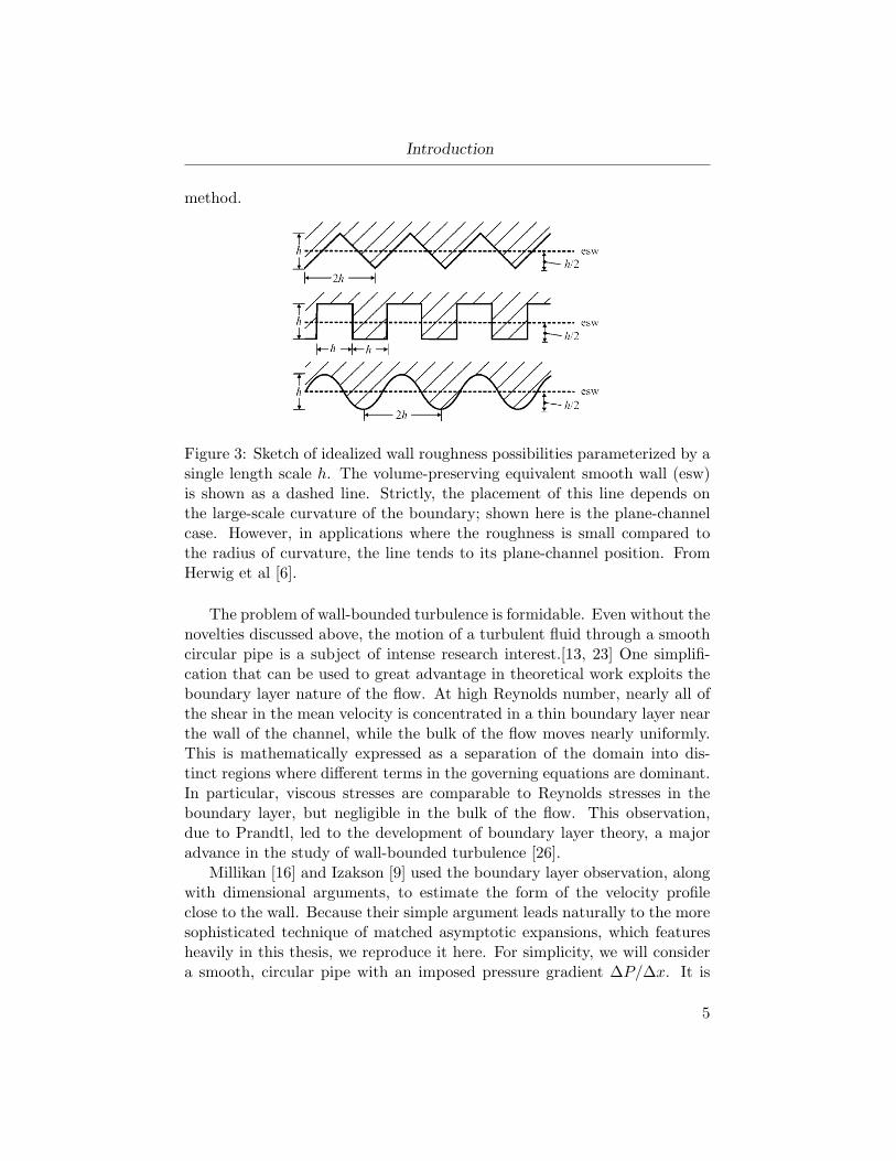
Even with a single roughness length scale, there are many ways of defin-ing the boundary of the idealized smoothed pipe. For a circular pipe, choos-ing the boundary is a one degree of freedom problem; engineers usually setthis “wall offset” by calibrating the velocity profile to a logarithmic form[28], as discussed below. However, it is preferable for the geometry to bedefined independently of flow data. Herwig [6] argued that a natural wayof placing the boundary is to ensure that the volume of the idealized pipeis equal to the volume of the true, rough pipe, as illustrated in Figure 3.Since this may easily be extended to non-circular pipes, we will adopt this
3An exception is river meandering, where the secondary flow advects sediment.4The effect of roughness type on the roughness parameters is reviewed in ([6, 10, 25]).
4
Introduction
method.
Figure 3: Sketch of idealized wall roughness possibilities parameterized by asingle length scale h. The volume-preserving equivalent smooth wall (esw)is shown as a dashed line. Strictly, the placement of this line depends onthe large-scale curvature of the boundary; shown here is the plane-channelcase. However, in applications where the roughness is small compared tothe radius of curvature, the line tends to its plane-channel position. FromHerwig et al [6].
The problem of wall-bounded turbulence is formidable. Even without thenovelties discussed above, the motion of a turbulent fluid through a smoothcircular pipe is a subject of intense research interest.[13, 23] One simplifi-cation that can be used to great advantage in theoretical work exploits theboundary layer nature of the flow. At high Reynolds number, nearly all ofthe shear in the mean velocity is concentrated in a thin boundary layer nearthe wall of the channel, while the bulk of the flow moves nearly uniformly.This is mathematically expressed as a separation of the domain into dis-tinct regions where different terms in the governing equations are dominant.In particular, viscous stresses are comparable to Reynolds stresses in theboundary layer, but negligible in the bulk of the flow. This observation,due to Prandtl, led to the development of boundary layer theory, a majoradvance in the study of wall-bounded turbulence [26].
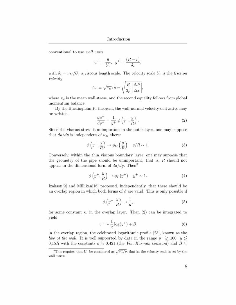
Millikan [16] and Izakson [9] used the boundary layer observation, alongwith dimensional arguments, to estimate the form of the velocity profileclose to the wall. Because their simple argument leads naturally to the moresophisticated technique of matched asymptotic expansions, which featuresheavily in this thesis, we reproduce it here. For simplicity, we will considera smooth, circular pipe with an imposed pressure gradient ∆P/∆x. It is
5
Introduction
conventional to use wall units
u+ =u
Uτ, y+ =
(R− r)δv
,
with δv = νM/Uτ a viscous length scale. The velocity scale Uτ is the frictionvelocity
Uτ ≡√τw/ρ =
√R
2ρ
∣∣∣∣∆P∆x
∣∣∣∣,where τw is the mean wall stress, and the second equality follows from globalmomentum balance.
By the Buckingham Pi theorem, the wall-normal velocity derivative maybe written
du+
dy+=
1y+
φ(y+,
y
R
). (2)
Since the viscous stress is unimportant in the outer layer, one may supposethat du/dy is independent of νM there:
φ(y+,
y
R
)→ φO
( yR
)y/R ∼ 1. (3)
Conversely, within the thin viscous boundary layer, one may suppose thatthe geometry of the pipe should be unimportant; that is, R should notappear in the dimensional form of du/dy. Then5
φ(y+,
y
R
)→ φI
(y+)
y+ ∼ 1. (4)
Izakson[9] and Millikan[16] proposed, independently, that there should bean overlap region in which both forms of φ are valid. This is only possible if
φ(y+,
y
R
)→ 1
κ, (5)
for some constant κ, in the overlap layer. Then (2) can be integrated toyield
u+ ∼ 1κ
log(y+) +B (6)
in the overlap region, the celebrated logarithmic profile [23], known as thelaw of the wall. It is well supported by data in the range y+ & 100, y .0.15R with the constants κ ≈ 0.421 (the Von Karman constant) and B ≈
5This requires that Uτ be considered as√τw/ρ; that is, the velocity scale is set by the
wall stress.
6
Introduction
5.6 [14]. For many applications, (6) is sufficient as a solution to the fluidproblem. This is primarily because as δv/R → 0, asymptotically all of theshear lies within the overlap region in which (6) is valid. One consequenceof this is that integrating (6) from the edge of the boundary layer to thecentre of the pipe gives an expression for mean velocity as a function ofboundary layer thickness (or Reynolds number) in excellent agreement withexperimental data [23]. This is true despite the fact that the argumentsleading to (6) are invalid near the centre of the pipe.
It is clear from the derivation that the assumption of a circular pipewas inessential. In fact, the universal form (6) is also observed in planechannels and slowly-growing flat plate turbulent boundary layers [23]. Fornon-circular pipes, sufficiently far from corners, a logarithmic profile for thewall-normal velocity is also observed, but the constants κ and B must bereplaced with functions of a coordinate running parallel to the wall, and themean wall stress should be replaced with its local value [1, 5, 20, 32].
Townsend [31] extended the Izakson-Millikan argument to the case ofrough walls, by proposing that the outer flow should not depend on theroughness length scale ks. The derivation is then entirely analogous, exceptthat B must be replaced by a function of the roughness Reynolds numberk+s = ksUτ/νM .6
The major fault of the above analysis is that no indication is given asto the accuracy of (6), or indeed why there should even be an overlap layerin which φ tends to a constant. To clarify these issues with the heuristicboundary-layer analysis initiated by Prandtl, in the 1950’s applied mathe-maticians developed the technique of matched asymptotic expansions [7]. Inthis, scaled, dimensionless equations are produced in the inner and outerregions, and a suitable small parameter is identified, usually a dimensionlessboundary layer thickness, δ. Since the regions are characterized by differentphysical balances, these equations will necessarily differ in their dependenceon δ.
The existence of a boundary layer implies that δ 1, so that solutionsmay be sought as asymptotic expansions in δ. In general, these solutionswill contain undetermined constants or functions, which are sought throughthe process of matching, which ensures that the solution varies smoothlyfrom the inner to the outer domain. In the language of matched asymptoticexpansions, the law of the wall is the velocity profile in the matching re-gion; the Izakson-Millikan argument produces the leading order behaviourby ensuring that it is possible to match the inviscid outer solution with the
6κ is observed to be universal, i.e., independent of k+s .
7
Introduction
geometry-independent inner solution.Several matching techniques exist. Introducing n, the dimensionless dis-
tance from the wall, the inner region is characterized by n . δ, while theouter region is n ∼ 1. The most general form introduces an intermediatecoordinate ζ such that ζ/n→ 0 and δ/ζ → 0 as δ → 0. Then, one imposesthe condition that, in ζ coordinates, the inner and outer solutions are equalas δ → 0. A simpler way of matching is Van Dyke’s rule, which states,loosely, that in the limit δ → 0, the inner expansion of the outer solutionshould equal the outer expansion of the inner solution.
The matched inner and outer solutions may be used to obtain a com-posite expansion that is asymptotically valid in the entire flow domain. Asimple prescription is to add the inner and outer solutions, and subtracttheir common part. As emphasized by Panton [22], the composite solutionis the best representation of the solution at relatively large δ. This is par-ticularly important when applied to a turbulent boundary layer, since theoft-used law of the wall is merely the common part of inner and outer solu-tions, and can be quite inaccurate as a velocity profile when δ is relativelylarge.
Matched asymptotic expansions were first applied to the problem of aturbulent boundary layer by Yajnik [33] and Mellor [15]. These authors didnot impose a turbulence closure, so that their solution is necessarily incom-plete. However, by assuming that the Reynolds stress admits an asymptoticexpansion of a particular form, they were able to reproduce several empiricalresults, including the law of the wall. This had the important effect of clar-ifying (6) as an asymptotic result, valid only in the limit δ → 0, and only ina limited range of n. When precise tests are made of the form of the veloc-ity profile, as in the Princeton Superpipe experiment [14], the distinction iscrucial. For example, deviations from the logarithmic profile have been inter-preted by some researchers as evidence for additional “meso”layers, which,physically, should represent different physical balances. However, these cor-rections can be more economically interpreted as higher order terms in astandard asymptotic expansion [34]. Not only does this simplify the phys-ical interpretation, but it also reduces the number of degrees of freedomwhich need to be constrained by data, since the corrections can be obtainedself-consistently from the governing equations.
These early works did not obtain a complete solution to the velocityprofile because no closure was imposed. However, they show that matchedasymptotic expansions are the natural tool with which to solve boundarylayer problems. In chapter 4, we will employ the technique to partially solvethe difficult problem of a turbulent boundary layer in a non-circular pipe.
8
Chapter 1
Governing Equations
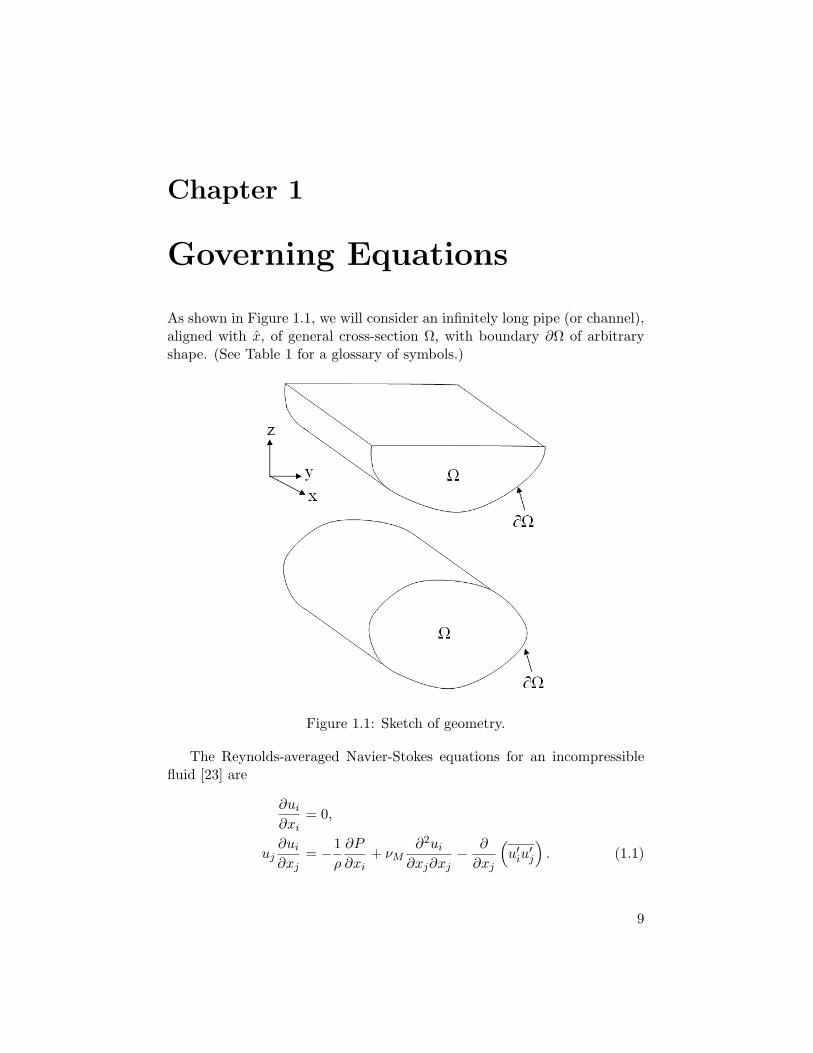
As shown in Figure 1.1, we will consider an infinitely long pipe (or channel),aligned with x, of general cross-section Ω, with boundary ∂Ω of arbitraryshape. (See Table 1 for a glossary of symbols.)
Figure 1.1: Sketch of geometry.
The Reynolds-averaged Navier-Stokes equations for an incompressiblefluid [23] are
∂ui∂xi
= 0,
uj∂ui∂xj
= −1ρ
∂P
∂xi+ νM
∂2ui∂xj∂xj
− ∂
∂xj
(u′iu′j
). (1.1)
9
Chapter 1. Governing Equations
In the above, and throughout, the Einstein summation convention is used,with indices running from 1 to 3 unless specified otherwise. Also, it will beconvenient to use the dual notation u = (u1, u2, u3) = (u, v, w) and x =(x1, x2, x3) = (x, y, z). As boundary conditions we will assume a prescribedaxial pressure gradient − |∆P/∆x| and the no-slip condition at the wall.
In the case of an open channel, we will assume that the free surface isflat, with normal z. In this case the vertical component of gravity is assumedalready absorbed into the pressure; the axial component gives rise to dP/dx.To simplify the discussion, we will only consider explicitly the case of a pipe.There is no loss of generality, since for any given channel, we can create anequivalent pipe by reflecting the channel shape about the free surface. Thestress-free condition then reduces to regularity of the solution along the axisof symmetry.
An important quantity not directly appearing in (1.1) is the wall stressτw, which must be defined as (ρνM∂u/∂y − ρu′v′) · n, in which y = (y, z),u′v′ ≡ u′v′ y+u′w′ z, and n is a dimensionless unit vector normal to the wall.The inclusion of Reynolds stresses here is necessary because, unlike the caseof a smooth wall, for a rough wall they need not vanish on the surface ∂Ω.Near the wall, the velocity scale is set by τw. Its mean value τw is known apriori since by integrating (1.1) over Ω, we see that |∂Ω| τw = −|Ω|∆P/∆x.The appearance here of the hydraulic radius R = 2|Ω|/|∂Ω| suggests that itis the relevant length scale for the outer region.
In fact, there is another important outer region length scale, more nat-urally used to scale the tranverse coordinates: the maximum distance fromthe wall, Nmax. As scales for nondimensionalizing the equations, the differ-ence between R and Nmax is merely cosmetic, but later we will propose aconstitutive relation for a turbulent mixing length. This should be, as muchas possible, independent of geometry. This can only be so in units madedimensionless by Nmax.7
We will consider fully developed flow, in which the velocity is independentof x [23]. Initially, we will seek a solution with non-zero velocity only in x,so that (u, v, w) = (u(y, z), 0, 0). This neglects the secondary flow, to whichwe will return in Chapter 4. Under these assumptions, one can show thatmomentum conservation in the transverse directions requires only that thepressure is constant through the cross-section. Since the continuity equationis satisfied identically, the only equation we need consider is conservation of
7For many shapes, such as squares, circles, and isosceles triangles, the two lengthscales are identical. The important exception is the infinite plane channel, for which thehydraulic radius is twice the maximum distance from the wall.
10
1.1. Scaling
streamwise momentum.
1.1 Scaling
Since the basic pipe flow results from the balance of the imposed pressuregradient with the Reynolds shear stresses, a natural choice for the velocityscale of turbulent fluctuations is
UT =
√R
2ρ
∣∣∣∣∆P∆x
∣∣∣∣ =√τw/ρ ≡ Uτ ,
the friction velocity. As a mean velocity scale, we will set U ≡ Uτ/κ, whereκ . 1 is treated as an empirical constant. For agreement with data, we willfind that κ = 0.421, the Von Karman constant.8
An appropriate scaling for the flow variables in the outer region is then
u = Uu∗, (u′, v′, w′) = UT (u′∗, v′∗, w
′∗), x = Lx∗,
(y, z) = Nmax(y∗, z∗), P =12
∣∣∣∣∆P∆x
∣∣∣∣LP∗, τw = ρU2T τw∗,
with L a streamwise length scale. Note that the fluctuating velocities havebeen scaled isotropically, in accordance with their assumed random nature.These scalings imply that the dimensionless mean wall stress is unity.
Immediately dropping the asterisk decoration, the dimensionless stream-wise momentum equation is
0 = 2ξ +∇ ·(−u′v′ + 1
κReτ∇u), (1.2)
where we have introduced the notation ∇ = ( ∂∂y ,
∂∂z ) and u′v′ ≡ u′v′ y +
u′w′ z. The dimensionless constants are
Reτ =UτNmax
νM, κ =
UTU, ξ =
Nmax
R.
For all turbulent flows, Reτ 1/κ, and the viscous term may safely beignored, in the outer region. However, as mentioned in the introduction, the
8Values are quoted in the range 0.37 to 0.43 [14]. It is clear from boundary layer con-siderations that we should use a value obtained at the largest possible Reynolds number.We will use the value determined in the Princeton Superpipe experiment at Re > 106,κ = 0.421.[14]
11
1.1. Scaling
shear is concentrated in a thin boundary layer near the wall, within whichvariables need to be rescaled to reflect different physics. Since rough walledturbulent flows are affected by viscosity in addition to roughness, to choosethe correct boundary layer rescaling we must first be precise about exactlywhich boundary layer is important.
For any wall-bounded turbulent flow, there is a viscous sublayer, adja-cent to the wall, in which viscous stresses dominate the Reynolds stresses.However, for a rough wall, this layer may be irrelevant to determining meanflow properties if the roughness length scale ks is much bigger than the vis-cous length scale νM/Uτ . In this case, drag on the flow is caused by pressuredifferences between the fore and aft sides of roughness elements; viscous dragis negligible. We will consider this hydraulically rough (or fully rough) limit.Then we can ignore the viscous stress entirely, even in the boundary layer.In this case, (1.2) reduces to
− 2ξ = ∇ · (−u′v′). (1.3)
The modifications due to viscosity are considered in Appendix D.Evidently, the turbulence model will depend on the roughness length
scale ks. We will use the simple scaling
ks = Nmaxks∗.
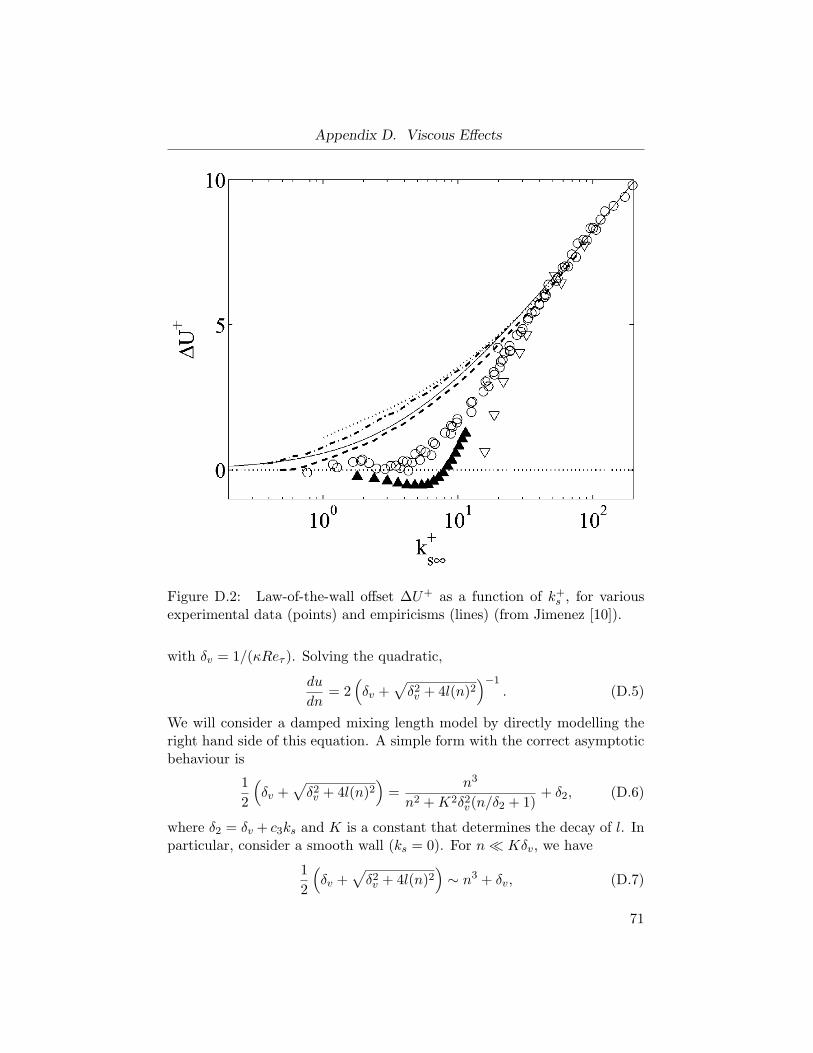
In the fully rough limit, the dimensionless boundary layer thickness δwill be proportional to ks: δ = cks. It is convenient to choose9 c ≈ 0.0279so that, for a circular pipe, the law of the wall takes the simple form10
u ∼ log(n/δ). (1.4)
We have derived (1.3) and justified neglect of the viscous term. To solve(1.3), we must now specify a turbulence closure.
90.0279 ≈ exp(−8.5κ)10This also requires that we choose κ ≈ 0.421
12
Chapter 2
Turbulence Closure
The simplest turbulence closure, due to Boussinesq [3], is the eddy viscositymodel
− (u′v′) = νT∇u, (2.1)
where now the eddy viscosity νT must be modelled. For a general flow, thisconstitutive assumption is not justified, and leads to erroneous results [23].However, for convectively steady problems, such as we are considering here,with appropriate modelling of νT , (2.1) is very successful [23].
Dimensionally, νT is the product of a velocity scale with a length scale.Adopting the eddy phenomenology of Kolmogorov [11], and making an anal-ogy with the molecular viscosity of a gas, Prandtl [24] proposed that thelength scale could be interpreted as a mixing length of dominant eddies, andthat the velocity scale could be obtained as the product of the local velocitygradient with the mixing length, viz.,11
νT = l2 |∇u| , (2.2)
where l is the mixing length. This implies the closure
− (u′v′) = l2 |∇u| ∇u. (2.3)
To specify l, Prandtl invoked a dimensional argument in analogy to Izakson-Millikan. There are five length scales in the problem: R, Nmax, n, νM/Uτ ,and ks. Prandtl proposed that there should be an overlap layer in which theonly available length scale is the distance to the wall, so that l ∝ n. It iseasily seen that this prescription implies the law of the wall, so that the over-lap layer can be identified with the matching region of the boundary layerstructure discussed in the introduction. Then, as in the Izakson-Millikanargument, in the fully turbulent outer layer, one would generally expect l tobe geometry-dependent. Conversely, in the boundary layer, l could dependon viscous or roughness length scales.
11We have generalized from the plane channel considered by Prandtl to an arbitraryshape by replacing |du/dy| with |∇u|
13
Chapter 2. Turbulence Closure
In the symmetric plane channel case considered by Prandtl, l is a func-tion of distance to the wall, since this is the only available coordinate. For anon-circular pipe, there is the possibility that l could depend on two trans-verse coordinates. However, the mixing length is interpreted as the size ofcharacteristic eddies – rotating, circular vortices. Since the distance fromthe wall, n(x), is the radius of the largest circle, centred at x, that is con-tained within the pipe, the identification of n with eddy size is natural andentirely independent of the cross-sectional shape. We may therefore stillexpect l = l(n).
Although heuristic, the mixing length approach has been very successfulin relating experimental results to eddy phenomenology [31]. For example,using a sensible parametrization of l derived from DNS data, L’vov andothers [13] have shown that the shear stress and mean velocity profiles ofcircular pipe and plane channel flow can be reproduced extremely accuratelywith few adjustable parameters. However, the closure (2.3) suffers froman important physical defect: as the centre of the pipe is approached, theReynolds shear stress tends to zero linearly, while the velocity gradient alsotends to zero linearly [22]. To satisfy (2.3), this forces the mixing lengthto diverge [13]. If l is truly a physically relevant quantity, this cannot bepermitted.
This can be alleviated by using an alternative velocity scale in the defi-nition of νT . Kolmogorov [11] proposed that the appropriate velocity scaleis provided by the turbulent kinetic energy, kT = u′2, so that νT = κkl
√kT ,
with κk a constant. To model kT , the turbulent energy equation is con-sidered under the approximation of local balance [13]. This implies thatproduction of turbulent energy, −u′v′ ·∇u, balances dissipation of turbulentenergy, εT . The latter is estimated as εT = κεk
3/2T /l, with κε a constant; this
may be taken as the definition of l. Defined in this way, l is well behavedthroughout the entire pipe. Then
νT = κkl√kT = κkl
(lεTκε
)1/3
= κν(l4εT )1/3, (2.4)
with κν = κk/κ1/3ε . Local balance of turbulent energy implies
εT = −u′v′ · ∇u = νT |∇u|2. (2.5)
Solving (2.4) and (2.5), we find
εT = κ3/2ν l2|∇u|3, νT = κ3/2
ν l2|∇u|. (2.6)
14
Chapter 2. Turbulence Closure
To match with known behaviour in the logarithmic region [23], we must takeκk ≈ 0.55, κε ≈ 0.553, so that κν = 1. Therefore, the prescription for νT isidentical to the original proposal, (2.3). However, here we used local balanceof turbulent energy, which is only strictly valid in the logarithmic region.Towards the centre of the pipe, the energy flux terms become important, sothat our algebraic model for energy balance breaks down. The failure of thealgebraic approximation leads to the divergence of l in (2.3). Fortunately,this has little impact on the mean velocity, which is nearly constant there.
Hitherto, all parameterizations of l have been intended for smooth-walledflows, for which the no-slip condition requires that l → 0 as n → 0.[23] Fora rough flow, we propose instead that l tends to a constant at the wall.Phenomenologically, eddies are prevented from decreasing in size indefinitelyby the roughness asperities at the wall.
Using the refined definition of l as κεk3/2T /εT , the mixing length is ob-
served in DNS data to saturate to a constant in the outer region.12 We willmodel this behaviour. A simple form with the desired properties is
l(n) ≡ n+ c3ks1 + c4n
, (2.7)
where ks is now dimensionless c4 & O(1) for the desired behaviour.With these constitutive relations, the streamwise momentum equation
takes the form
− 2ξ = ∇ ·
((n+ c3ks1 + c4n
)2
|∇u| ∇u
). (2.8)
12In direct numerical simulation, the Reynolds stress can be computed directly from thefluctuating velocity fields u′ and v′, so that the implied profile of mixing length can befound by rearranging (2.4).
15
Chapter 3
Circular Pipe Solution
To calibrate the constants c3 and c4 with well-verified empirical relations,we now solve (1.3) in the case of a fully rough circular pipe, using matchedasymptotic expansions. To maintain continuity with earlier arguments andwith later analysis, as a coordinate we use the (dimensionless) distance fromthe wall, n, which is related to the usual (dimensionless) radial coordinater by n = 1− r. In this case, (1.3) with (2.3) and (2.7) becomes
− 2 =1
1− nd
dn
((1− n)
(n+ c3/c δ
1 + c4n
)2 ∣∣∣∣dudn∣∣∣∣ dudn
). (3.1)
Since variables have been scaled for the outer (fully turbulent) region, wenaıvely pose an outer solution
u = u0 + δu1 + · · · .
Inserting this into (3.1) and integrating once, we find the leading orderequation ∣∣∣∣du0
dn
∣∣∣∣ du0
dn=
(1− 2n+ n2 + C0)(1 + c4n)2
n2(1− n). (3.2)
At the centre of the pipe, n = 1 and du/dn = 0, so that the integrationconstant C0 = 0. Assuming du0/dn > 0 and integrating again, the outerregion velocity is
u0 = log(
1−√
1− n1 +√
1− n
)+ 2√
1− n− 23c4(1− n)3/2 + C1, (3.3)
where the constant C1 needs to be determined by matching with the bound-ary layer. To determine the inner (boundary-layer) equations, we need torescale the variables n and u. Near the wall, the velocity scale is set bythe wall stress, so that the appropriate scale is the friction velocity Uτ .Therefore, an appropriate rescaling in the boundary layer is
N =1δn, U = u, (3.4)
16
Chapter 3. Circular Pipe Solution
leading to
− 2δ =1
1− δNd
dN
((1− δN)
(N + c3/c
1 + c4δN
)2 ∣∣∣∣ dUdN∣∣∣∣ dUdN
). (3.5)
LettingU = U0 + δU1 + · · ·
as above, we find
C2 = (N + c3/c)2
∣∣∣∣dU0
dN
∣∣∣∣ dU0
dN. (3.6)
At N = 0, the wall stress is unity in outer variables, so that C2 = 1.Assuming dU0/dN > 0 and integrating, we find the inner solution
U0 = log(cN
c3+ 1), (3.7)
where, by the no-slip condition, there is no integration constant. Solutions(3.3) and (3.7) need to be matched. We will apply Van Dyke’s rule, whichstates that the outer expansion of the inner solution must equal the innerexpansion of the outer solution. The former is
u0m = log(cn
c3δ
)+O(δ) (3.8)
Expressed in outer variables, the inner expansion of the outer solution is
u0m = log(n
4
)+ 2− 2
3c4 + C1 +O(δ log δ). (3.9)
To obtain agreement to O(δ log δ), we should take C1 = log(4c/c3δ)−2+ 23c4.
As mentioned in the introduction, the leading order velocity profile in thematching region is the law of the wall. Therefore, comparing (3.8) with(1.4), we see that c3 = c ≈ 0.0279. This calibrates the wall-offset constantc3.
The appearance of log(δ) in C1 indicates that our original expansion foru was not quite correct: written as an explicit asymptotic series in δ, wehave, in the outer region,
u0 = − log(δ) +[log(
1−√
1− n1 +√
1− n
)+ 2(√
1− n− 1)
−23c4((1− n)3/2 − 1) + log(4)
]. (3.10)
17
Chapter 3. Circular Pipe Solution
The leading order term, − log(δ), is asymptotically different from 1 as δ → 0.Since we have only made asymptotic expansions in one dependent variable,there is no need to revise the expansion and match again. Note that theleading order contribution is produced entirely in the boundary layer.
To calibrate the constant c4, which determines the saturation of l(n)for large n, we need to use a quantity sensitive to the velocity in the outerregion. A suitable measure is the friction factor, a dimensionless measure ofmean velocity[23]:
f ≡∣∣∣∣∆P∆x
∣∣∣∣ 4RρU2〈u0〉2Ω
(3.11)
=8κ2
〈u0〉2Ω. (3.12)
Computation of 〈u0〉Ω requires integrating the solution over the entire flowdomain. For this purpose, a composite solution is invaluable. The additivecomposite solution resulting from (3.3) and (3.7) is
u0c = log(
1 +δ
n
)+ log
(1−√
1− n1 +√
1− n
)+ 2√
1− n− 23c4(1− n)3/2 + C1.
(3.13)Using u0c in f , we find
f = 8κ2
[1π
∫ 2π
0
∫ 1
0(1− n) u0c(n) dn dθ
]−2
(3.14)
= 8κ2
[−16
15− 8c4
21+ log
(4δ
)− 2 +
2c4
3+O(δ log δ)
]−2
(3.15)
=[
12√
2κ
(log(
4cks
)− 46
15+
6c4
21+O(δ log δ)
)]−2
. (3.16)
The experimental result, due to Nikuradse [21] and later improved by Schlicht-ing [26], is
f =[2.00 log10
(1ks
)+ 1.74
]−2
. (3.17)
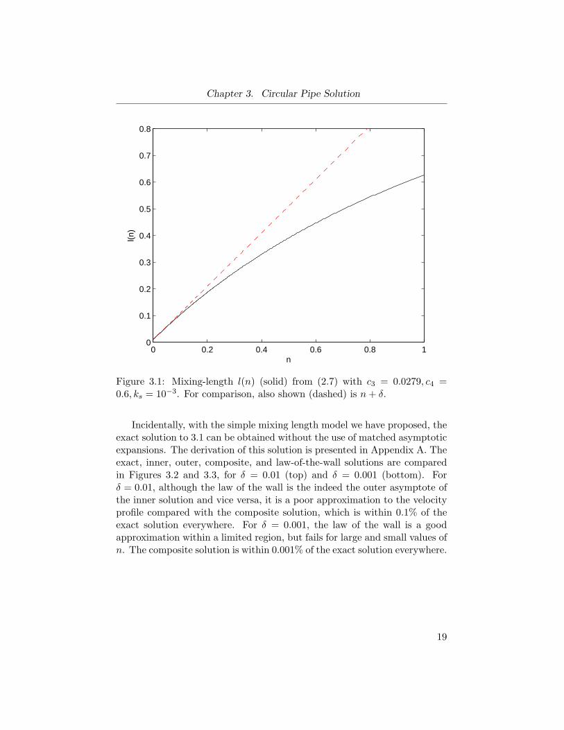
We can obtain agreement to O(δ log δ) if we take13 c4 = 0.6. This completescalibration of the turbulence model. The resulting prescription for the mix-ing length is shown in Figure 3.1. Analogous results and computations fora plane channel are given in Appendix C.
13Note that log(10)/(2√
2κ) ≈ 1.93 for κ = 0.421. Better agreement can be obtained byusing κ = 0.406, but it seems preferable to obtain agreement with the newest data; thatis, with the Superpipe experiment that yields κ = 0.421 [14, 29].
18
Chapter 3. Circular Pipe Solution
0 0.2 0.4 0.6 0.8 10
0.1
0.2
0.3
0.4
0.5
0.6
0.7
0.8
n
l(n)
Figure 3.1: Mixing-length l(n) (solid) from (2.7) with c3 = 0.0279, c4 =0.6, ks = 10−3. For comparison, also shown (dashed) is n+ δ.
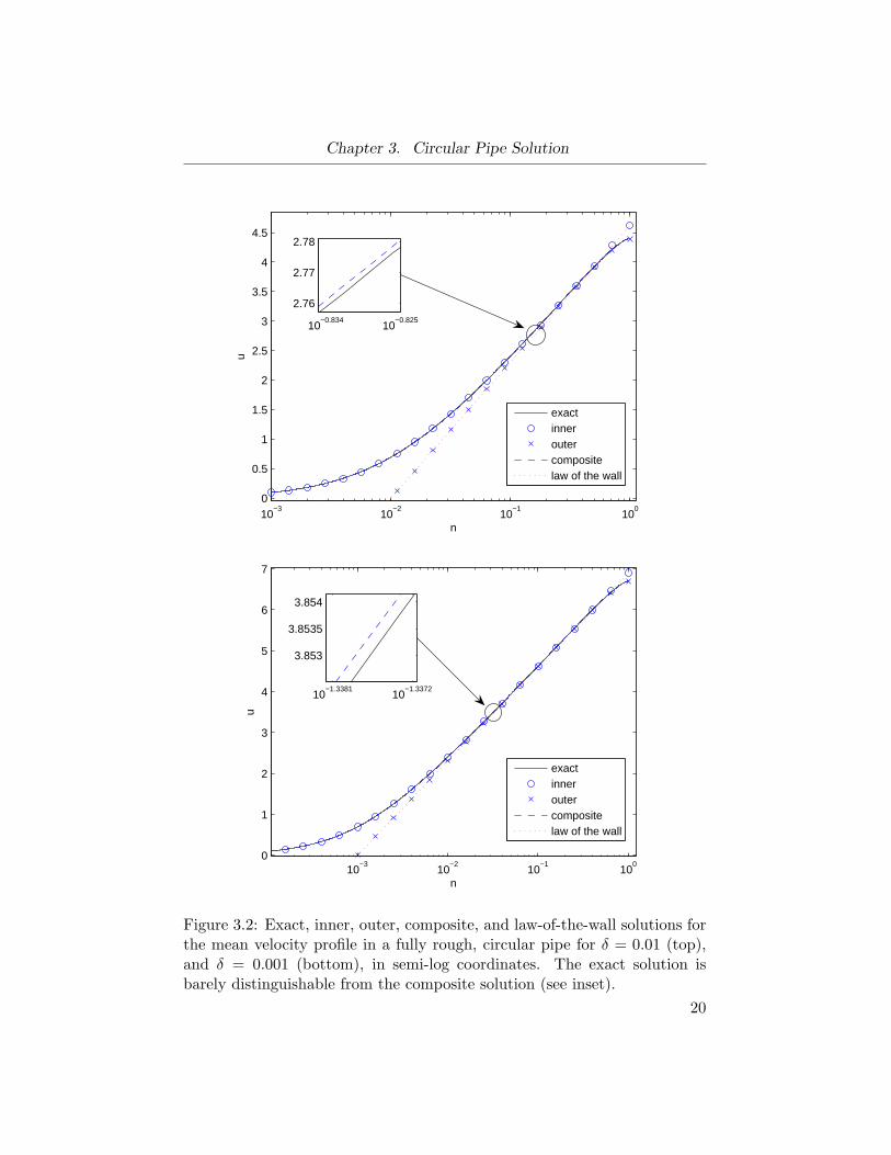
Incidentally, with the simple mixing length model we have proposed, theexact solution to 3.1 can be obtained without the use of matched asymptoticexpansions. The derivation of this solution is presented in Appendix A. Theexact, inner, outer, composite, and law-of-the-wall solutions are comparedin Figures 3.2 and 3.3, for δ = 0.01 (top) and δ = 0.001 (bottom). Forδ = 0.01, although the law of the wall is the indeed the outer asymptote ofthe inner solution and vice versa, it is a poor approximation to the velocityprofile compared with the composite solution, which is within 0.1% of theexact solution everywhere. For δ = 0.001, the law of the wall is a goodapproximation within a limited region, but fails for large and small values ofn. The composite solution is within 0.001% of the exact solution everywhere.
19
Chapter 3. Circular Pipe Solution
10−3
10−2
10−1
100
0
0.5
1
1.5
2
2.5
3
3.5
4
4.5
n
u
exactinneroutercompositelaw of the wall
10−0.834
10−0.825
2.76
2.77
2.78
10−3
10−2
10−1
100
0
1
2
3
4
5
6
7
n
u
exactinneroutercompositelaw of the wall
10−1.3381
10−1.3372
3.853
3.8535
3.854
Figure 3.2: Exact, inner, outer, composite, and law-of-the-wall solutions forthe mean velocity profile in a fully rough, circular pipe for δ = 0.01 (top),and δ = 0.001 (bottom), in semi-log coordinates. The exact solution isbarely distinguishable from the composite solution (see inset).
20
Chapter 3. Circular Pipe Solution
0 0.2 0.4 0.6 0.8 10
0.5
1
1.5
2
2.5
3
3.5
4
4.5
n
u
exactinneroutercompositelaw of the wall
0.594 0.596 0.5984.068
4.07
4.072
4.074
4.076
0 0.2 0.4 0.6 0.8 10
1
2
3
4
5
6
7
n
u
exactinneroutercompositelaw of the wall
0.518 0.52
6.235
6.24
6.245
Figure 3.3: Exact, inner, outer, composite, and law-of-the-wall solutions forthe mean velocity profile in a fully rough, circular pipe for δ = 0.01 (top),and δ = 0.001 (bottom). The exact solution is barely distinguishable fromthe composite solution (see inset).
21
Chapter 4
An Approximation Schemefor Non-Circular Pipes
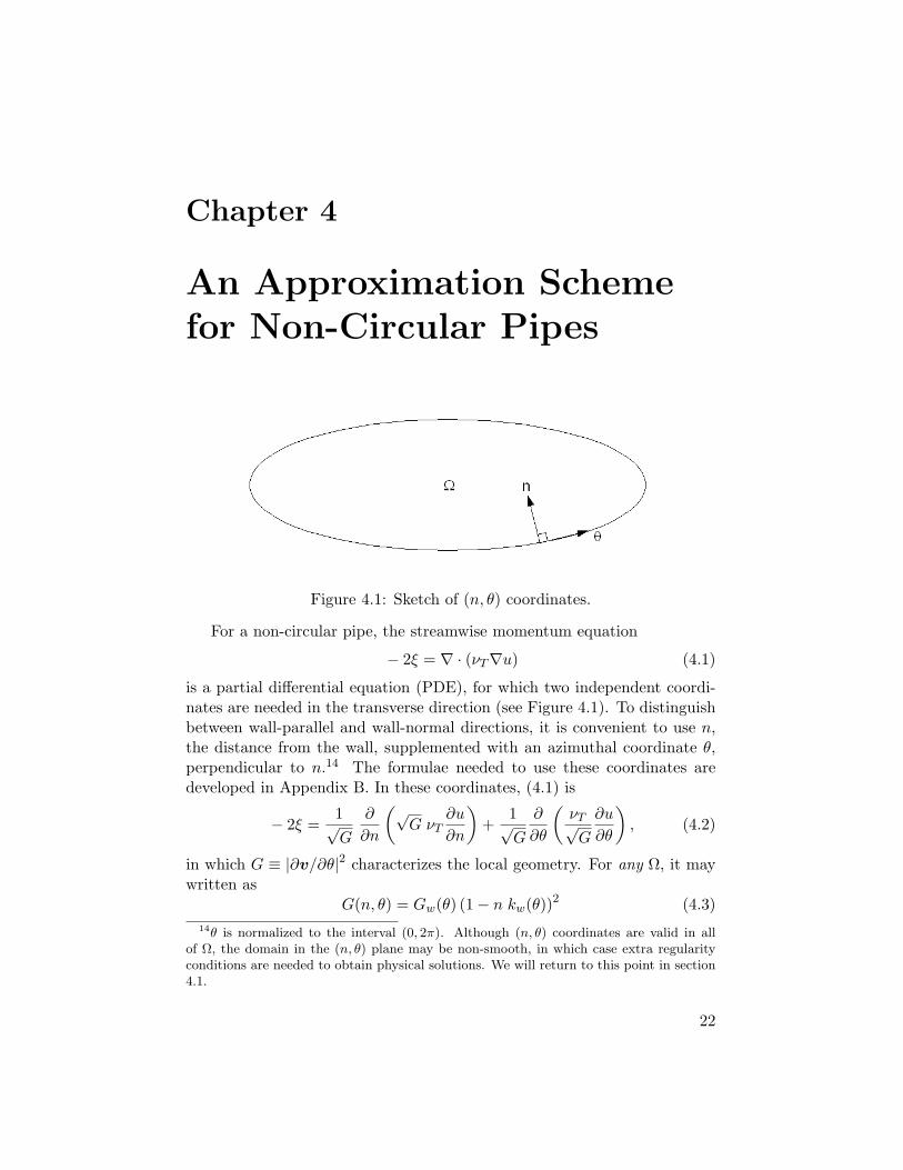
Figure 4.1: Sketch of (n, θ) coordinates.
For a non-circular pipe, the streamwise momentum equation
− 2ξ = ∇ · (νT∇u) (4.1)
is a partial differential equation (PDE), for which two independent coordi-nates are needed in the transverse direction (see Figure 4.1). To distinguishbetween wall-parallel and wall-normal directions, it is convenient to use n,the distance from the wall, supplemented with an azimuthal coordinate θ,perpendicular to n.14 The formulae needed to use these coordinates aredeveloped in Appendix B. In these coordinates, (4.1) is
− 2ξ =1√G
∂
∂n
(√G νT
∂u
∂n
)+
1√G
∂
∂θ
(νT√G
∂u
∂θ
), (4.2)
in which G ≡ |∂v/∂θ|2 characterizes the local geometry. For any Ω, it maywritten as
G(n, θ) = Gw(θ) (1− n kw(θ))2 (4.3)14θ is normalized to the interval (0, 2π). Although (n, θ) coordinates are valid in all
of Ω, the domain in the (n, θ) plane may be non-smooth, in which case extra regularityconditions are needed to obtain physical solutions. We will return to this point in section4.1.
22
Chapter 4. An Approximation Scheme for Non-Circular Pipes
in terms of its value at the wall, Gw, and the wall curvature, kw. Thetransformations that lead to equations (4.2) and (4.3) are given in AppendixB. For a circular pipe, kw = 1, while for a plane channel, kw = 0.
Equation (4.2) is a difficult nonlinear partial differential equation. Evenusing matched asymptotic expansions, in general the outer problem mustbe solved numerically. We have done so with COMSOL, a finite elementpackage. These numerical solutions are used to validate the approxima-tions developed below. Instead of relying entirely on numerical solutions,by examining the boundary layer structure of the problem, we can motivateapproximate methods of solution. We will return to this after consideringthe boundary layer problem.
To rescale for the inner region, we supplement (3.4) with V = νT /δ.Then, (4.2) becomes
− 2ξδ =1√G
∂
∂N
(√GV
∂U
∂N
)+
δ2
√G
∂
∂θ
(V√G
∂U
∂θ
). (4.4)
From this we see that, to O(δ), only the wall-normal turbulent flux is im-portant. Posing a solution
U = U0 + δU1 + · · · ,
we findτw(θ) = V
∂U0
∂N(4.5)
with V = (N + 1)2∣∣∣∂U0∂N
∣∣∣+O(δ). The equation
τw(θ) = (N + 1)2
∣∣∣∣∂U0
∂N
∣∣∣∣ ∂U0
∂N(4.6)
is then the boundary layer equation analogous to (3.6).15 The importantdifference is that τw is now an unknown function of θ. Equation (4.6) can,of course, be integrated to
U0 =√τw(θ) log(N + 1). (4.7)
Recall that U was nondimensionalized with the friction velocity Uτ =√τw/ρ.
From (4.7) we see that the appropriate velocity scale is actually the local fric-tion velocity
√τw(θ)/ρ. Therefore, to leading order, azimuthal dependence
15Recall that C2 = 1, c3 = c.
23
Chapter 4. An Approximation Scheme for Non-Circular Pipes
in the boundary layer is restricted to the variation of wall stress, which setsthe appropriate velocity scale.
The critical simplification that has allowed us to find a solution to theboundary layer problem is neglect of the term involving ∂U/∂θ, which rep-resents the Reynolds shear stress along θ. This simplification turns (4.2)from a partial differential equation into an ordinary differential equation,with parametric θ dependence. This is justified by the small thickness ofthe boundary layer in comparison to relevant transverse length scales. Inthe outer layer, there is no such separation of length scales. However, thereare several heuristic reasons to expect that the most important variation ofu is along rays of constant θ, that is,
∇u ≈ ∂u
∂n∇n, (4.8)
a “radial” approximation.First, the streamwise velocity is empirically known to increase mono-
tonically from the wall to the centre of the pipe, where the velocity is, ofcourse, independent of direction. This geometrical constraint suggests thatazimuthal variation is maximal near the wall, where (4.8) is asymptoticallyvalid.
Second, we have already motivated a mixing length turbulence model inwhich the mixing length l depends only on n, the distance from the wall.Physically, this corresponds to the identification of l as the size of dominanteddies. In this model, azimuthal dependence is expected to derive fromgeometrical quantities that vary between rays of constant θ; namely, wallcurvature, kw(θ), and the maximum distance from the wall, nmax(θ). Forcross-sectional shapes with these quantities weakly varying, (4.8) may be agood approximation.
It is important to recall that we have neglected the secondary flow. Thesecondary flow adds important “non-radial” physics that raises serious doubtabout the validity of (4.8). We will comment further on this below.
24
Chapter 4. An Approximation Scheme for Non-Circular Pipes
Applying (4.8) to (4.1), and using (B.14) from Appendix B, we have
−2ξ = ∇ ·(νT∂u
∂n∇n)
= ∇ ·(νT∂u
∂nen
)=
1√G
∂
∂n
(√GνT
∂u
∂n
)=
11− kw(θ)n
∂
∂n
((1− kw(θ)n)l(n)2
∣∣∣∣∂u∂n∣∣∣∣ ∂u∂n
). (4.9)
It is easy to see that we could have obtained this equation directly from(4.11) by neglecting the turbulent shear stress along eθ. Integrating thisequation, ∣∣∣∣∂u∂n
∣∣∣∣ ∂u∂n =τ(n, θ)
1− kw(θ)n
(1 + c4n
n
)2
, (4.10)
where we have introduced the reduced stress
τ(n, θ) = τw(θ)− 2ξn+ ξkw(θ)n2.
In exceptional cases, we may have ∂u/∂n < 0. However, the approximationswe will later make require ∂u/∂n ≥ 0. Therefore,
u(n, θ) = C +∫ n
0
√τ(n′, θ)√
1− kw(θ)n′
(1 + c4n
′
n′
)dn′. (4.11)
The constant C is determined by matching to the boundary layer solution(4.7).
Assuming the validity of this functional form for u, the remaining “bound-ary condition” that determines the unknown function τw(θ) is regularity ofthe solution in the outer region. In particular, u and ∇u should be smooththroughout the outer region. This is guaranteed everywhere except alongthe curve n = nmax(θ), where the coordinates are discontinuous. (see Figure4.2) Along this curve, we must therefore prescribe the jump conditions
[u]+− = 0,[∂u
∂y
]+
−= 0,
[∂u
∂z
]+
−= 0. (4.12)
The three conditions are not independent, since [u]+− = 0 implies that thetangential component of ∇u is continuous along the curve. Therefore, we
25
Chapter 4. An Approximation Scheme for Non-Circular Pipes
only need to impose differentiability of u normal to the curve. In fact, thesystem formed by equations (4.11) and (4.12) form an integro-differentialequation that is not amenable to solution without further approximation. Tomake progress, we will consider two alternative methods of approximation.The first is to approximate the form of u, and apply the exact boundarycondition (4.14), while the second is to directly approximate an expressionfor the reduced stress τ . Because these are uncontrolled approximations,they must be duly tested with any given geometry.
To focus the discussion, it is helpful to restrict attention to a family ofgeometries collectively known as anisotropic superellipses. These are shapesparameterized by∣∣∣y0
a
∣∣∣my +∣∣∣z0
b
∣∣∣mz = 1 ⇔y0 = a | cos(θ)|2/my sgn(cos(θ))z0 = b | sin(θ)|2/mz sgn(sin(θ))
. (4.13)
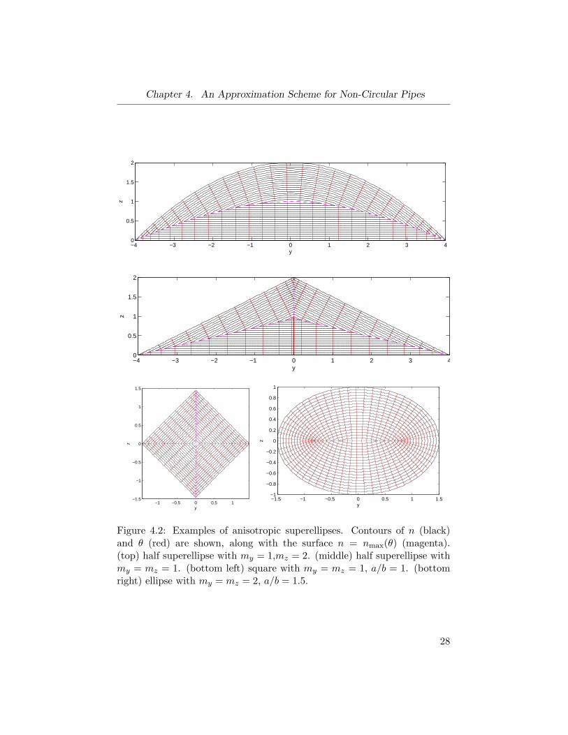
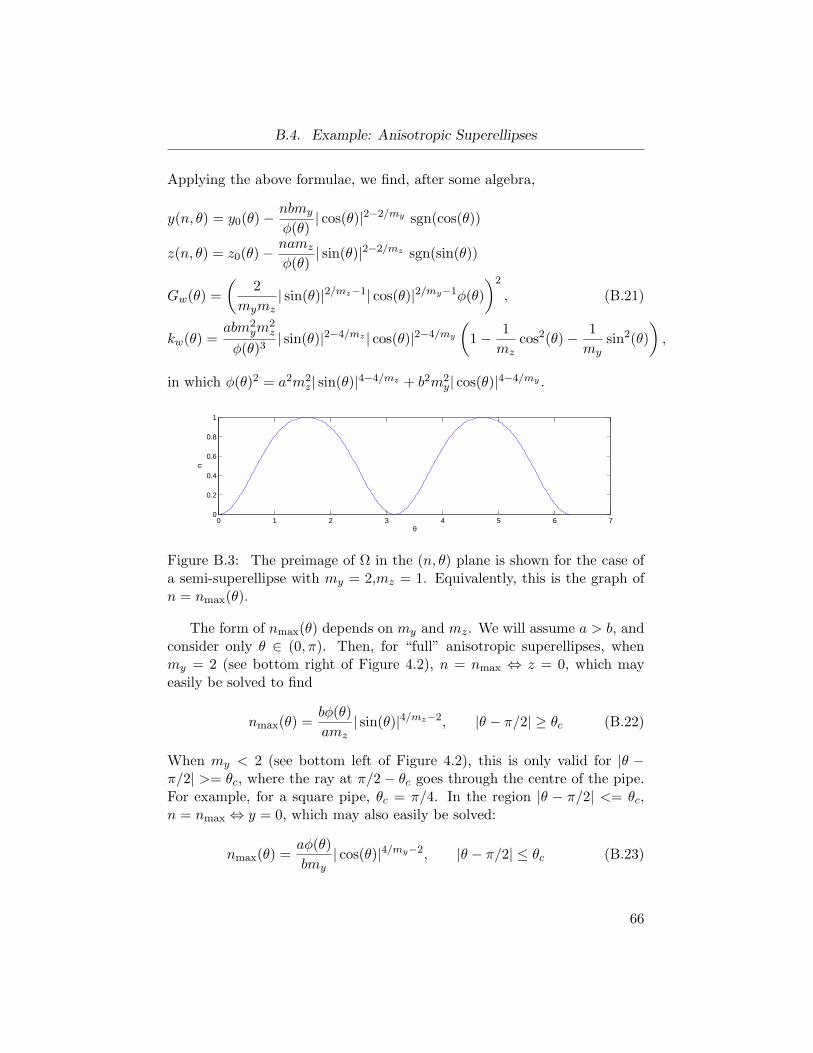
We will let 0 < my,mz ≤ 2. As special cases, this family includes ellipses(my = mz = 2) and diamonds (my = mz = 1). A plane channel is re-produced in the singular limit mz = 2, b/a → 0. We will let the shapeeither be “full”, parameterized by θ ∈ (0, 2π), or “semi”, where θ ∈ (0, π),and the bottom of the shape is the line z = 0. (see Figure 4.2) The formercovers a wide variety of pipe shapes, and, through the symmetry argumentmentioned earlier, a variety of realistic open-channel shapes. The “semi”shapes are reasonable pipe shapes for many geophysical applications [18].16
The formulae for y(n, θ), z(n, θ), Gw(θ), kw(θ), and nmax(θ) can all beanalytically derived for anisotropic superellipses. These results are presentedin Appendix B.
We will apply the first approximation, which uses (4.12), only to shapesthat are symmetric about the curve n = nmax(θ). All “full” anisotropicsuperellipses are of this type. In this case, the jump conditions (4.12) sim-plify. Continuity of u is guaranteed, and instead of requiring no jump inthe u derivative normal to the curve n = nmax(θ), we have instead that thederivative vanishes. Therefore, the jump conditions become local boundaryconditions. Restricting our attention to one side of the curve, we may con-sider n = nmax(θ) as the level set of n−nmax(θ). Then, setting the derivative
16We have normalized by the maximum distance from the wall. Therefore, for a “full”shape, 1 = min(a, b).
26
Chapter 4. An Approximation Scheme for Non-Circular Pipes
normal to the curve to zero, we have17
0 = ∇(n− nmax(θ)) · ∇u
=∂u
∂n− 1G
dnmax(θ)dθ
∂u
∂θ. (4.14)
17Here we use the fact that |∇n| = 1, |∇θ| = 1/√G; see Appendix B.
27
Chapter 4. An Approximation Scheme for Non-Circular Pipes
y
z
−4 −3 −2 −1 0 1 2 3 40
0.5
1
1.5
2
y
z
−4 −3 −2 −1 0 1 2 3 40
0.5
1
1.5
2
y
z
−1 −0.5 0 0.5 1−1.5
−1
−0.5
0
0.5
1
1.5
y
z
−1.5 −1 −0.5 0 0.5 1 1.5−1
−0.8
−0.6
−0.4
−0.2
0
0.2
0.4
0.6
0.8
1
Figure 4.2: Examples of anisotropic superellipses. Contours of n (black)and θ (red) are shown, along with the surface n = nmax(θ) (magenta).(top) half superellipse with my = 1,mz = 2. (middle) half superellipse withmy = mz = 1. (bottom left) square with my = mz = 1, a/b = 1. (bottomright) ellipse with my = mz = 2, a/b = 1.5.
28
4.1. Constant-stress Approximation
4.1 Constant-stress Approximation
For circular pipes at small boundary layer thicknesses, the logarithmic pro-file is a reasonable approximation to the velocity profile throughout the outerregion, although the arguments leading to it are invalid there (see Figure3.2). Indeed, it is used in many engineering applications when more sophis-ticated analysis is unwarranted. Therefore, a simple ansatz for the velocityprofile in a non-circular pipe is to extend the logarithmic profile into theouter region, viz.,
u0 =√τw(θ) log
(nδ
). (4.15)
It is simple to check that this results from (4.11) under neglect of wallcurvature, mixing length saturation, and pressure gradient. Whereas in acircular pipe the logarithmic profile is associated with constant stress [31],in a non-circular pipe, (4.15) is associated with stress constant along eachray of constant θ. Substituting (4.15) into the boundary condition (4.14),after some re-arranging, leads to
d
dθlog(τw) = 2Gw(1− kwnmax)2
(nmax
dnmax
dθlog(nmax
δ
))−1
, (4.16)
and therefore determination of τw is reduced to quadrature. The constantof integration is set by the requirement of unit mean wall stress.
A well-known shortcoming of the logarithmic profile is that it has a non-zero slope at the centre of the pipe, which is forbidden by regularity.18 It iseasy to see from (4.14) that this may lead to problems in a non-circular pipe.In particular, if dnmax/dθ = 0 somewhere, then 1/G du0/dθ is required todiverge. This severely restricts the applicability of the logarithmic profileapproximation. However, for shapes where dnmax/dθ 6= 0 everywhere, (4.16)is often a good approximation. To illustrate, we will derive an explicitexpression for τw for a square pipe, and compare this with the DNS data ofHuser and Biringen.[8]
18For circular pipes, this is one reason to prefer a solution of the type presented inChapter 3.
29
4.1. Constant-stress Approximation
4.1.1 Square Pipe
By symmetry, we can restrict our discussion to the region θ ∈ (0, π/2). Fora square pipe19, kw = 0 and Gw(θ) = 4 sin2(2θ). Then for θ < π/4,
n = nmax(θ)⇔ z = 0
⇔ nmax(θ) = 2 sin2(θ), (4.17)
using (B.22) from Appendix B. Similarly, for θ ∈ (π/4, π/2), we have nmax(θ) =2 cos2(θ). Substituting these expressions into (4.16) and integrating, we find
τw(θ) = τ0
[log(nmax(θ)
δ
)]2
, (4.18)
where the constant τ0 is set by the requirement that 〈τw〉∂Ω = 1. There is aminor problem with this expression: for nmax < δ the result is an unphysicaldivergence of the wall stress. This indicates that there is a corner boundarylayer. Since the approximations made do not warrant a rigorous treatment,a simple fix, inspired by (4.7), is to replace nmax/δ by nmax/δ + 1. Theapproximate solution for u0 is then
u0(n, θ) =√τ0 log
(nmax(θ)
δ+ 1)
log(nδ
+ 1). (4.19)
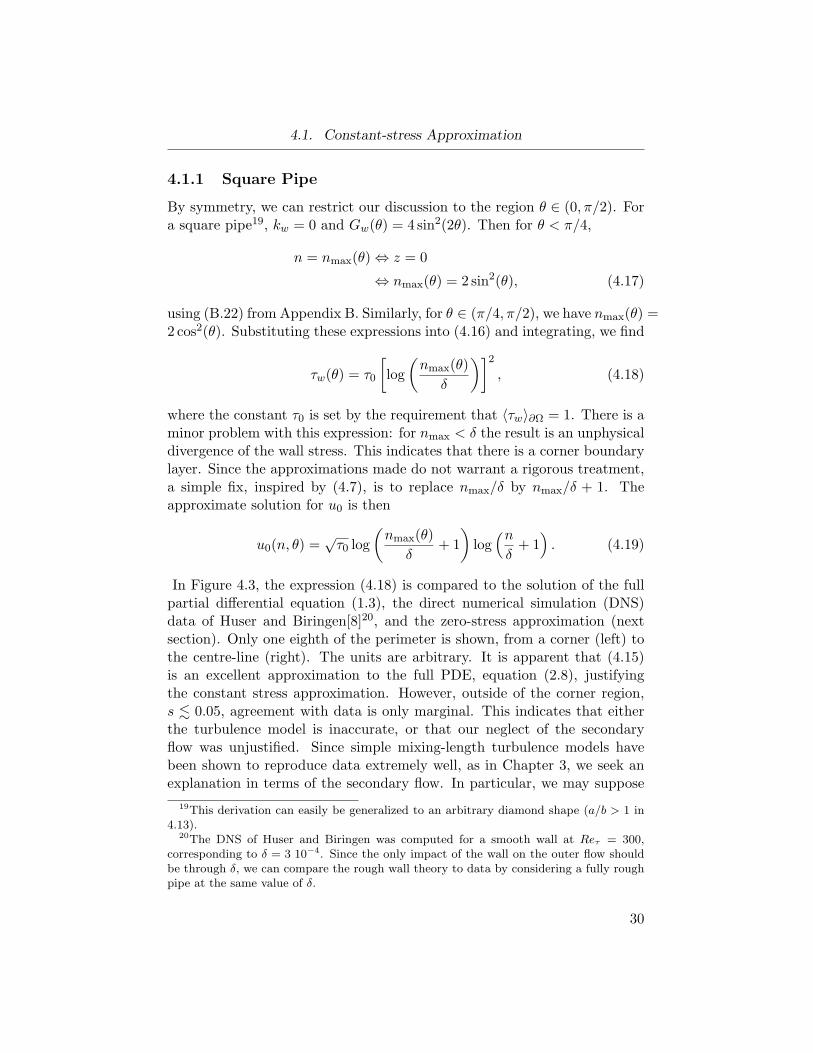
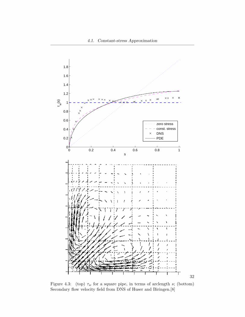
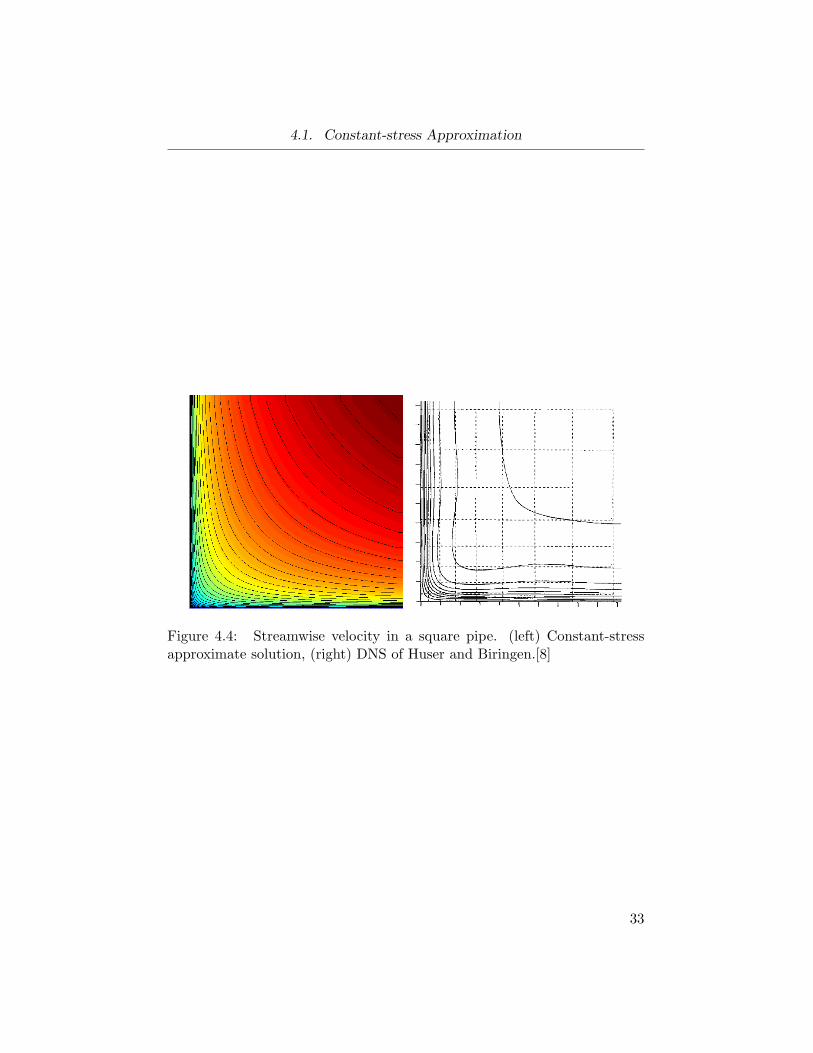
In Figure 4.3, the expression (4.18) is compared to the solution of the fullpartial differential equation (1.3), the direct numerical simulation (DNS)data of Huser and Biringen[8]20, and the zero-stress approximation (nextsection). Only one eighth of the perimeter is shown, from a corner (left) tothe centre-line (right). The units are arbitrary. It is apparent that (4.15)is an excellent approximation to the full PDE, equation (2.8), justifyingthe constant stress approximation. However, outside of the corner region,s . 0.05, agreement with data is only marginal. This indicates that eitherthe turbulence model is inaccurate, or that our neglect of the secondaryflow was unjustified. Since simple mixing-length turbulence models havebeen shown to reproduce data extremely well, as in Chapter 3, we seek anexplanation in terms of the secondary flow. In particular, we may suppose
19This derivation can easily be generalized to an arbitrary diamond shape (a/b > 1 in4.13).
20The DNS of Huser and Biringen was computed for a smooth wall at Reτ = 300,corresponding to δ = 3 10−4. Since the only impact of the wall on the outer flow shouldbe through δ, we can compare the rough wall theory to data by considering a fully roughpipe at the same value of δ.
30
4.1. Constant-stress Approximation
that the velocity (u, 0, 0) is only the leading order term in a more completesolution that includes the secondary flow. The latter is induced because wallstress variations are unstable to isotropizing perturbations [31].
Therefore, the secondary flow is in such a direction as to minimize wallstress variation. This is corroborated by the data presented in Figures 4.4and 4.3. Since the wall stress must be zero at the corner and have unit mean(shown as a dashed line), one expects that as δ → 0, τw will increase itsslope at the corner. This is predicted by equation (4.18). Also, consider theintersection of the DNS data with the theoretical curves. To the left of thispoint, the secondary flow has increased the wall stress, so u should increaseand the flow should be converging toward the wall. This is supported by theDNS data. (see Figure 4.4) Note, in particular, that the intersection pointis aligned with the centre of the lower secondary flow vortex.
31
4.1. Constant-stress Approximation
0 0.2 0.4 0.6 0.8 10
0.2
0.4
0.6
0.8
1
1.2
1.4
1.6
1.8
s
τ w(s
)
zero stressconst. stressDNSPDE
Figure 4.3: (top) τw for a square pipe, in terms of arclength s; (bottom)Secondary flow velocity field from DNS of Huser and Biringen.[8]
32
4.1. Constant-stress Approximation
Figure 4.4: Streamwise velocity in a square pipe. (left) Constant-stressapproximate solution, (right) DNS of Huser and Biringen.[8]
33
4.2. Zero-stress Approximation
4.2 Zero-stress Approximation
In a circular pipe and plane channel, the shear stress decreases linearlyfrom the wall to the centre-line, where it vanishes. A simple approximationfor a general Ω, assuming (4.8), is therefore to let the analogous quantity,the reduced stress τ(n, θ), vanish on n = nmax(θ). It may be seen from(4.10) that this implies ∂u/∂n = 0 on n = nmax(θ), which may or may notbe a good approximation to (4.14), depending on Ω. This gives a simpleexpression for the wall stress,
τw(θ) = ξ nmax(θ) (2− kw(θ)nmax(θ)) , (4.20)
which should be contrasted with (4.18). In particular, note that, here, τwhas no δ dependence. Also, there are no adjustable constants. Fortunately,
|∂Ω|〈τw(θ)〉∂Ω =∫ 2π
0
(2ξ nmax(θ)− ξkw(θ)n2
max(θ))ds
= 2ξ∫ 2π
0
(nmax(θ)− 1
2kw(θ)n2
max(θ)) √
Gw(θ) dθ
= 2ξ∫ 2π
0
∫ nmax(θ)
0(1− nkw(θ))
√Gw(θ) dn dθ
= 2ξ∫ 2π
0
∫ nmax(θ)
0
√G(n, θ) dn dθ
= 2ξ|Ω|.
In dimensionless terms, ξ = |∂Ω|/(2|Ω|), so that 〈τw(θ)〉∂Ω = 1, as desired.This identity is an indication that (4.20) is a sensible approximation.
To find the velocity profile, we will ignore the minor effect of wall cur-vature, noting that the same velocity profile results for a circular pipe andplane channel (see Appendix C). Then the integral (4.11) can be computedanalytically:
u(n, θ) = C +∫ n
0
√τ(n′, θ)(1 + c4n
′)n′
dn′
= C + 2√τ(n, θ)
(1− c4τ(n, θ)
3ξ
)−√τw log
(√τw +
√τ(n, θ)
√τw −
√τ(n, θ)
).
(4.21)
This matches to the inner solution when
C = −2√τw
(1− c4τw
3ξ
)−√τw log
(2τwδ
).
34
4.2. Zero-stress Approximation
To illustrate, we consider an elliptical pipe.
4.2.1 Elliptical Pipe
For an elliptical pipe with a > b = 1,
kw(θ) =8aφ(θ)3
, Gw(θ) =φ(θ)2
4, nmax(θ) =
φ(θ)2a
, (4.22)
in terms of φ(θ) =√
4a2 sin2(θ) + 4 cos2(θ). Then, after some manipulation,
τw(θ) =ξ
a
(1 + 2(a2 − 1) sin2(θ))√a2 sin2(θ) + cos2(θ)
. (4.23)
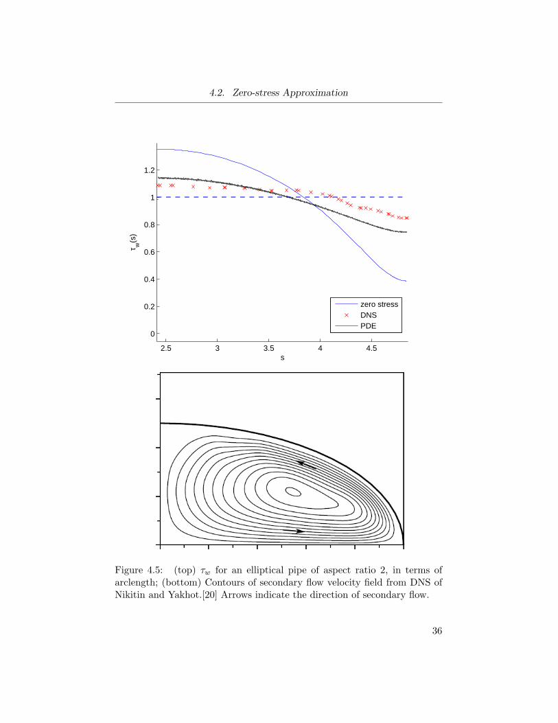
In Figure 4.2.1, this approximation is compared to the solution of the fullPDE (2.8), and to the DNS of Nikitin and Yakhot.[20]21 Although thequalitative behaviour of the approximation is correct, it overestimates theanisotropy of τw by more than a factor of two compared to the PDE. ThePDE is a reasonable approximation to the DNS, but it too overestimates theanisotropy of τw. As with the square pipe, this can be explained in termsof the secondary flow, which is directed towards the elongated end of theellipse. Owing to the absence of corners, here the secondary flow is less pro-nounced. The velocity distributions from the PDE and DNS are comparedin Figure 4.6.
21The DNS was performed for a smooth wall at Reτ = 157, corresponding to δ =6× 10⁻⁴. Again, we consider the equivalent fully rough wall.
35
4.2. Zero-stress Approximation
2.5 3 3.5 4 4.5
0
0.2
0.4
0.6
0.8
1
1.2
s
τ w(s
)
zero stressDNSPDE
Figure 4.5: (top) τw for an elliptical pipe of aspect ratio 2, in terms ofarclength; (bottom) Contours of secondary flow velocity field from DNS ofNikitin and Yakhot.[20] Arrows indicate the direction of secondary flow.
36
4.2. Zero-stress Approximation
Figure 4.6: Streamwise velocity in an elliptical pipe. (top) Solution of fullPDE, (bottom) DNS of Nikitin and Yakhot.[20]
37
4.2. Zero-stress Approximation
4.2.2 Semi-Elliptical Pipe
Semi-superellipses with my = 2 (see top of Figure 4.2) have dnmax/dθ = 0at the centre of the pipe, and therefore will not admit the constant-stressapproximation. Fortunately, for these shapes, the zero-stress approximationis very accurate. For general mz and b = 2, we have
kw(θ) =4am2
z
φ(θ)3| sin(θ)|2−4/mz
(2− 2
mzcos2(θ)− sin2(θ)
),
nmax(θ) =2| sin(θ)|2/mz
1 +amz
φ(θ)| sin(θ)|2−2/mz
(4.24)
in terms of φ(θ) =√a2m2
z| sin(θ)|4−4/mz + 16 cos2(θ). The implied formulafor τw = ξnmax(2− kwnmax) does not simplify very much. For mz = 1, it iscompared in Figure 4.7 to the solution of the PDE (2.8). Agreement is quitegood. There are no DNS results for this shape, but we can imagine that thesecondary flow would reduce the anisotropy in τw, in a similar manner as inthe square pipe.
2 4 6 8 10 12 14 160
0.2
0.4
0.6
0.8
1
1.2
1.4
1.6
s
τ w(s
)
zero stressPDE
Figure 4.7: τw for a semi-elliptical pipe of aspect ratio 2, with linear cor-ners, in terms of arclength. The left half corresponds to the top half of theboundary.
38
Chapter 5
The Thermal Problem
For many geophysical problems involving turbulent flow, in addition to thevelocity distribution it is necessary to obtain the temperature distributionin the flow and heat fluxes into the wall. As an application of the model, so-lutions and methods of the previous chapters, we will pose the heat transferproblem in a non-circular pipe and develop an approximation scheme, withan eye toward applications in glaciology.
In particular, floods under, through, or adjacent to glaciers involve theflow of turbulent water through a conduit or channel of ice [4]. Owing tomelting at the conduit wall, the conduit shape may evolve down the flowpath. If the length scale along which the conduit evolves is much longerthan its hydraulic radius, then the infinite pipe assumption considered inthis thesis may be appropriate. In this case, one would like to know the heatflux at the wall, so that the melt rate can be determined, and, therefore, theevolution of the conduit shape. The situation may be novel from a physicalpoint of view because, in the case of a subglacial flood, the water is onlyinfinitesimally warmer than the surrounding ice. This affects the relevantphysics, as explained below.
In many ways, the thermal problem is analogous to the mechanical prob-lem. Molecular diffusion of heat, which may be neglected in the core of theturbulent flow, is important at the wall, leading to a thermal boundarylayer. Since the thermal problem depends on the velocity field, this is com-plicated by the presence of the viscous boundary layer. For a smooth wall,the boundary layer thickness depends on the thermal diffusivity of the fluid;when the Prandtl number Pr = α/νM
22 is greater than unity, the thermalboundary layer is located within the viscous boundary layer, and universalbehaviour is observed [27].
For a rough wall, there are three boundary layers. In the fully roughregime, this actually simplifies the problem, because the most importantproperties of the velocity and temperature distributions are determined bythe same roughness boundary layer– at least, in the context of the simplest
22α is the thermal diffusivity of the fluid.
39
5.1. Scaling
turbulent heat flux models. We will consider this situation.As before, we decompose the temperature into mean and fluctuating
components, viz.,T = T + T ′. (5.1)
We perform the Reynolds-averaging procedure and drop the bar decora-tion immediately. The resulting Reynolds-averaged energy equation for anincompressible fluid is
cpuj∂T
∂xj= ε+ εT + cpα
∂2T
∂xj∂xj− cp
∂
∂xj
(u′jT
′). (5.2)
In these equations, ε and εT are the viscous energy and turbulent energydissipations, given by
ε =12νM
(∂ui∂xj
+∂uj∂xi
)2
, εT =12νM
(∂u′i∂xj
+∂u′j∂xi
)2
. (5.3)
The dissipation terms are often neglected, but they are important in glacio-logical applications; we will, therefore, retain them. As a model for εT , wewill use the simple model23 discussed in Chapter 2,
εT = l2|∇u|3. (5.4)
We are interested in the heat flux at the wall, which must be defined as
qw ≡ −ρcwα∂T
∂n+ ρcwu′nT
′, (5.5)
in terms of the inward facing normal n.
5.1 Scaling
We will introduce separate scales for the mean flow and turbulent fluctua-tion temperatures. The former is measured from a datum T0, which we willassume is the temperature at the pipe boundary. To determine the scale
23It should be noted that this model for εT can also be motivated by considering theReynolds-averaged Navier Stokes equations as modelling a complex fluid. Then, usingmethods of continuum mechanics, one may derive the implied energy equation. Thedissipation term that results is εT .
40
5.1. Scaling
for turbulent temperature fluctuations, ∆TT , we will assume that the tur-bulent energy flux balances the turbulent dissipation. The former scales ascpUT∆TT /Nmax, while the latter scales as24 (κNmax)2(U/Nmax)3. Thus
∆TT =Nmax
cpUT
((κNmax)2
(U
Nmax
)3)
=κU2
cp, (5.6)
where we have used κ = UT /U . This is an unusual situation, not oftenconsidered in the literature. It is relevant for the glaciological applicationbecause the water temperature in subglacial conduits does not deviate muchfrom 0oC. For example, consider a subglacial flood with water running at10m/s. Then the above scaling predicts ∆TT ∼ 0.01K.
The mean flow temperature scale, ∆T , is assumed proportional to theturbulent scale, viz., ∆T = (PrT /κ)∆TT . The turbulent Prandtl number,PrT , is an empirical constant, usually taken in the range 0.7-0.9 [27].
Scaling the new variables
T = T0 + ∆T T∗, T ′ = ∆TT T ′∗, qw = ρcpUT∆TT qw∗
ε = νMU2
N2max
ε∗, εT =UU2
T
NmaxεT∗, (5.7)
and dropping asterisks leads to the dimensionless energy equation
γPrTκ2
u∂T
∂x=
1κ2Reτ
ε+ εT −∇ · v′T ′ − γ∂
∂xu′T ′
+PrT
PrReτκ2
(∇2T + γ2∂
2T
∂x2
). (5.8)
The new dimensionless numbers are
γ =Nmax
L, PrT = κ
∆T∆TT
, P r =α
νM. (5.9)
We will assume fully rough conditions, so that the terms involving Reτ canbe dropped. Then, to complete the model, a turbulence closure for the tur-bulent heat fluxes must be specified. An expedient model often consideredin the literature is the natural extension of the eddy viscosity hypothesis,
v′T ′ = −νT∇T, u′T ′ = −γνT∂T
∂x. (5.10)
24Note that l ∼ κNmax.
41
5.1. Scaling
Physically, the assumption is that the same turbulent motion that advectsvelocity fluctuations also advects temperature fluctuations; therefore, theircorrelations should take an analogous form, with the same eddy viscosity.They may differ by a constant of proportionality; this has been incorporatedin PrT . With these assumptions, (5.8) becomes
γPrTκ2
u∂T
∂x= εT +∇ · (νT∇T ) + γ2νT
∂2T
∂x2(5.11)
This is a linear, inhomogeneous problem for the temperature field T . Fur-thermore, we know that u, νT and εT are independent of x. We thereforeseek a solution in the form
T = T (y, z) + eλx T (y, z), (5.12)
which is consistent with the homogeneous boundary conditions on T on∂Ω.25 The first component, T , contains the effect of dissipative heating onthe temperature field, and satisfies
∇ · (νT∇T ) = −l2|∇u|3. (5.13)
Evidently, this operates independently of the streamwise advection of heat.By integrating this equation over Ω, we see that the mean wall heat flux dueto dissipation is
〈qw〉Ω =−1|∂Ω|
∫ΩνT∇u · ∇u dS
=−1|∂Ω|
∫∂Ωu νT∇u · n dl +
1|∂Ω|
∫Ωu ∇ · (νT∇u) dS
=−2ξ|∂Ω|
∫Ωu dS
=−2√
2κf
, (5.14)
where f = 8κ2/〈u〉Ω is the friction factor. This identity is a consequenceof conservation of energy among the three levels of description: mean flow,turbulent fluctuations, and heat. In particular, the imposed pressure gradi-ent supplies energy to the mean flow; this is converted to turbulent kineticenergy by straining of the Reynolds stress along velocity gradients; turbu-lent energy is dissipated into heat; all the heat must escape at the wall asheat flux.
25To solve a given physical problem, in general a superposition of solutions is necessary.That is, eλx T must be replaced by
∫Aλe
λx Tλ dλ.
42
5.1. Scaling
The temperature field due to advection, T , satisfies
∇ · (νT∇T ) =λγPrTκ2
uT + γ2λ2νT T . (5.15)
In the treatment of the velocity problem, we have already implicitlyassumed that γ 1. Since we also have κ ≤ 1, the streamwise diffusion termis much smaller than the advection term and may be discarded. If γ κ2,as we expect, then both terms involving ∂T/∂x may be discarded, and T isunnecessary. However, to facilitate comparison with the dissipation-inducedtemperature field, we note that T (y, z) satisfies
∇ · (νT∇T ) = cλuT , (5.16)
with cλ = λγPrT /κ2.
The equations governing νT∇T and νT∇T should be contrasted. Theformer will be largest where u is – namely, near the centre of the pipe –whereas the latter will be largest where gradients of u are large, namely, inthe boundary layer.
As with the momentum problem, we will first seek solutions for a circularpipe.
43
5.2. Circular Pipe
5.2 Circular Pipe
For a circular pipe, (5.13) becomes
d
dn
((1− n)l(n)2dT
dn
∣∣∣∣dudn∣∣∣∣) = −(1− n)l(n)2
∣∣∣∣dudn∣∣∣∣3 . (5.17)
We will use the technique of matched asymptotic expansions. Posing a naiveexpansion
T = T0 + δT1 + · · · , (5.18)
we find the leading order outer problem
d
dn
((1− n)3/2n
(1 + c4n)dT0
dn
)= −(1− n)5/2(1 + c4n)
n, (5.19)
which can be integrated to
dT0
dn= −(1 + c4n)
r3/2n
[C1 + log
(1−√r
1 +√r
)+ 2√r +
23r3/2 +
25r5/2 − 2
7c4r
7/2
].
(5.20)Here, we have used r = 1−n to shorten some of the expressions. Finite heatflux at n = 1 (r = 0) requires that C1 = 0. This can again be integrated, to
T0 =C2 −12
[log(
1−√r
1 +√r
)]2
− 2(1 + c4)√r
log(
1−√r
1 +√r
)−(
1615− 16c4
7
)log(n)−
(25− 20c4
21
)r +
1235c4r
2 − 221c2
4r3. (5.21)
The constant C2 needs to be determined by matching to the boundary layersolution.
For a fully rough pipe, the thickness of the thermal boundary layer isproportional to ks, just like the momentum boundary layer. Therefore,we may use the same boundary layer rescaling n = δN . Denoting thetemperature in the boundary layer by TI , we will expand TI as
TI = TI0 + δTI1 + · · · , (5.22)
giving the leading order equation
d
dN
((N + 1)
dTI0dN
)= − 1
N + 1. (5.23)
44
5.2. Circular Pipe
HencedTI0dN
=−qw − log(N + 1)
N + 1, (5.24)
which can be integrated to
TI0 = −qw log(N + 1)− 12
[log(N + 1)]2 . (5.25)
Since T = 0 on n = 0, there is no integration constant. Matching with VanDyke’s rule, as N →∞, this becomes
TI0 ∼ −qw log(nδ
)− 1
2
[log(nδ
)]2+O(δ log(δ)2) (5.26)
This must be equated to the inner expansion of the outer solution,
T0 ∼ C2 −12
[log(n
4
)]2− 2(1 + c4) log
(n4
)−(
1615− 16c4
7
)log(n)
−(
25− 20c4
21
)+
1235c4 −
221c2
4 +O(δ). (5.27)
This implies
qw = log(δ) + c6, C2 =12
log(δ)2 + c6 log(δ) + c7, (5.28)
where c6 and c7 are δ-independent constants.26 One may easily check thatthe identity (5.14) is satisfied.
To find these solutions, we neglected advection. In reality, the dissipatedheat produced in the outer core of the flow is advected downstream, so thatthe temperature at the centre of the pipe continually increases. For ourneglect of advection to be sound, we would hope that the bulk of dissipatedheat is produced in the boundary layer and diffused out at the boundary. It istherefore worth considering the distribution of dissipation. We will consideran artificial separation of Ω into n < δη, and n > δη, with 0 < η < 1, sothat the separation is in the matching region. Denoting the contributionof dissipation in the boundary layer and outer region by QBL, and QO,
Which contribution is greater depends on the value of η. For 0 < η < 1/2,QBL > QO, while for η > 1/2, QBL < QO. This sensitive dependenceon η indicates that most of the dissipation occurs in the matching region.As δ → 0, this region tends toward the wall, so that, indeed, most of thedissipation is produced near the wall.
Heat transfer results are usually presented as a heat transfer coefficient,or Stanton number correlation.27 Abusing notation, this is, in dimensionalterms, St = −qw/(cp〈u〉(T (n = 1) − T (n = 0))). We will use an overbar
27Note that St = Nux/(RexPr), where Nux and Rex are the Nusselt and Reynoldsnumbers determined by an arbitrary length scale x, and Re is determined with the meanvelocity.
46
5.2. Circular Pipe
to indicate that this is for the dissipation-induced temperature field. In ournotation, we have
As δ → 0, the term in parentheses tends to unity, giving a simple form forSt.
Although there are accepted engineering relations for St, most are in-tended for smooth wall flows, where the Prandtl number plays a criticalrole in determining the relative size of thermal and viscous boundary layers.More importantly, accepted heat transfer relations are for advection domi-nated temperature fields. Still, it is useful to compare the relations. We willdenote these advection-induced Stanton numbers by St.
A simple relation for high Re that follows from the Izakson-Millikanargument, applied to the thermal problem, is [27]
St = f/(8PrT ) (5.32)
Engineers favour the Dittus-Boelter equation28
St = 0.023(
2ξ
√8fReτPr
3
)−1/5
. (5.33)
Since the Prandtl number appears here as the ratio of viscous and thermalboundary layer thicknesses for a smooth wall, the most straightforward wayto extend this result to rough walls is to set Pr = 1 and replace Reτ withexp(−κB)/δ.
28This is usually presented as Nu = 0.023Re0.8Pr0.4, where the Nusselt and Reynoldsnumbers are based on the hydraulic diameter, and the Reynolds number is based on themean velocity.
47
5.2. Circular Pipe
10−6
10−5
10−4
10−3
10−2
10−1
10−4
10−3
10−2
10−1
100
101
δ
St
Present modelIzakson−MillikanDittus−Boelter
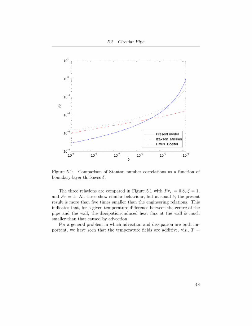
Figure 5.1: Comparison of Stanton number correlations as a function ofboundary layer thickness δ.
The three relations are compared in Figure 5.1 with PrT = 0.8, ξ = 1,and Pr = 1. All three show similar behaviour, but at small δ, the presentresult is more than five times smaller than the engineering relations. Thisindicates that, for a given temperature difference between the centre of thepipe and the wall, the dissipation-induced heat flux at the wall is muchsmaller than that caused by advection.
For a general problem in which advection and dissipation are both im-portant, we have seen that the temperature fields are additive, viz., T =
48
5.3. Non-Circular Pipe
T + eλxT .29 Therefore, the Stanton number is
St = −κ√f/8
PrT
qw + eλxqw
T (n = 1) + eλxT (n = 1)
= −κ√f/8
PrT
[qw
T (n = 1)
(T (n = 1)
T (n = 1) + eλxT (n = 1)
)
+qw
T (n = 1)
(eλxT (n = 1)
T (n = 1) + eλxT (n = 1)
)]
= St
(T (n = 1)
T (n = 1) + eλxT (n = 1)
)+ St
(eλxT (n = 1)
T (n = 1) + eλxT (n = 1)
)(5.34)
This indicates that the Stanton numbers for the dissipation and advectioninduced temperature fields are additive, provided they are weighted with thetemperature difference carried by each field. As indicated by the factor eλx,this will depend on the downstream distance. In particular, sufficiently fardownstream, if λ > 0, the advection effects should dominate, while if λ < 0,dissipation will dominate.
5.3 Non-Circular Pipe
The difficulties that appear in solving the thermal problem in a non-circularpipe are analogous to those earlier dealt with for the velocity problem. Ac-cordingly, we will follow the same procedure in determining approximatesolutions, and omit some details. We will neglect streamwise advection ofheat. In (n, θ) coordinates, (5.13) is
1√G
∂
∂n
(√G νT
∂T
∂n
)+
1√G
∂
∂θ
(νT√G
∂T
∂θ
)= −l2|∇u|3. (5.35)
Again, we attempt solution with matched asymptotic expansions. We willfirst consider the boundary layer problem. Writing TI = TI0 + δTI1 + · · ·for the solution in the inner region, the leading order problem is
∂
∂N
((N + 1)
√τw(θ)
∂TI0∂N
)=−τw(θ)3/2
N + 1. (5.36)
29As earlier, for a general problem eλx must be replaced by∫Aλe
λxdλ.
49
5.3. Non-Circular Pipe
Hence∂TI0∂N
=−qw(θ)√
τw(θ)(N + 1)− τw(θ)N + 1
log(N + 1), (5.37)
which may be integrated to
TI0 =−qw(θ)√τw(θ)
log(N + 1)− τw(θ)2
[log(N + 1)]2. (5.38)
An immediate consequence of this expression is that the wall heat flux mustvanish whenever the wall stress does. Like the wall stress in the mechanicalproblem, the wall heat flux must be determined by matching to the outerproblem.
The general outer problem is intractable. As before, we have found nu-merical solutions with COMSOL, a finite element package. These solutionsare compared to analytical results in what follows.
To make analytical progress, we will employ similar approximations asin chapter 4. Proceeding as before, we will discard the explicit θ derivatives.Then, (5.35) becomes an ordinary differential equation in n with parametricθ dependence. Integrating once,
q ≡ −νT∂T
∂n= −C(θ)√
G+
1√G
∫ n
0
√G l2
∣∣∣∣∂u∂n∣∣∣∣3 dn′. (5.39)
Here, q is a reduced heat flux, analogous to the reduced stress of the mo-mentum problem. The unknown function C(θ) must be related to qw bymatching, and then determined by regularity of the solution in the outerregion. As before, we will only consider this regularity condition explicitlyfor symmetric shapes. In this case, on n = nmax(θ), T satisfies
0 =∂T
∂n− 1G
dnmax(θ)dθ
∂T
∂θ. (5.40)
The system of equations (5.39) and (5.40) is still too difficult to solve an-alytically. Therefore, as in the momentum problem, we will first considerapproximating the velocity and temperature fields, and applying the exactboundary condition.
5.3.1 Constant Heat Flux Approximation
For the same reasons as in chapter 4, a reasonable and simple ansatz forthe form of the temperature field is to assume that the inner solution isvalid in the outer region, that is, to use equation (5.35). Physically, this
50
5.3. Non-Circular Pipe
corresponds to assuming a constant heat flux in the outer region. If makingthis assumption, it is reasonable to also assume that the velocity takes theanalogous form, (4.15). Then, note that
T0 =−qw√τw
log(nδ
+ 1)− 1
2u2
0. (5.41)
Under these assumptions, (5.40) becomes
0 =−qw√τw
1nmax
− 1G
dnmax
dθlog(nδ
+ 1) ∂
∂θ
(−qw√τw
)− u0
(∂u0
∂n− 1G
dnmax
dθ
∂u0
∂θ
). (5.42)
This is a first order, linear equation in qw/√τw, whose solution can im-
mediately be written down. However, if we assume that the wall stress isdetermined by (4.14), as is consistent with the assumed form of u0, then thesource term vanishes identically, and we see that qw/
√τw satisfies the same
equation as√τw. Since the equation admits the trivial scaling symmetry,
we have, immediately,−qw√τw∝√τw.
Setting the constant of proportionality so that the correct mean wall heatflux is attained, we have
qw =−2√
2κf
τw, (5.43)
a surprising result, considering that the temperature and velocity fields dif-fer. This result allows the solutions for τw from Section (4.1) to be im-mediately applied. As an example, in Figure 5.2, qw for a square pipe, aspredicted by (5.43), is compared to the solution of the full PDE (5.13). Theagreement is very good.
5.3.2 Zero Heat Flux Approximation
An alternative approximation, analogous to letting the reduced stress vanishon n = nmax, is to let the reduced turbulent heat flux q vanish there. Toobtain an expression for q, we need to compute the dissipation integral in(5.39). A simple approximation that makes this possible is again to ignorethe minor effect of wall curvature. Then
q = −C(θ)√Gw− c4
5ξτ5/2 +
23τ3/2 + 2τw
√τ − τ3/2
w log
(√τw +
√τ
√τw −
√τ
), (5.44)
51
5.3. Non-Circular Pipe
0 0.1 0.2 0.3 0.4 0.5 0.6 0.7 0.8 0.90
0.2
0.4
0.6
0.8
1
1.2
s
q w(s
) / <
q w>
PDEConstant Heat Flux
Figure 5.2: Heat flux in a square pipe, normalized by its mean. One eighthof the pipe boundary is shown. The corner is at right.
with τ = τw − 2ξn the approximate reduced wall stress. This must bematched to the outer asymptote of the inner solution (5.37),
qI0 ∼ qw + τ3/2w log
(nδ
). (5.45)
HenceC√Gw
= −qw −c4
5ξτ5/2w +
23τ3/2w + 2τ3/2
w − τ3/2w log
(2τwξδ
). (5.46)
Letting q = 0 when τ = 0, we find30 C = 0 and therefore
qw(θ) = −τ3/2w
(log(
2τwξδ
)+c4
5ξτw −
83
). (5.47)
30This is slightly inconsistent, in that we earlier assumed that τ = 0 on n = nmax.We cannot make that assumption here, because (5.44) requires τ ≥ 0. The best way toproceed would be to retain τ in the dissipation integral. This can be done, also somewhatinconsistently, by ignoring only the effect of wall curvature in the denominator of ∂u/∂n.This leads to a much longer formula for q, without much improving the approximation.
52
5.3. Non-Circular Pipe
In Figure 5.3, this approximation is tested for a semi-superellipse againstthe full PDE (5.13). Agreement is only slightly worse than the accuracy ofthe τw approximation (see Figure 4.7).
2 4 6 8 10 12 14 160
0.5
1
1.5
2
s
q w(s
) / <
q w>
PDEZero Heat Flux
Figure 5.3: Heat flux in a semi-elliptical pipe, normalized by its mean.
53
Chapter 6
Conclusion
In this thesis, we have considered turbulent flow in a rough pipe of arbitraryshape. Although many engineering problems fall into this category, theseare usually of a few standard shapes, such as the square pipe, which havebeen extensively studied. Instead, we focus on the universal aspects of theproblem, so that solutions may be obtained in evolving geometries, as occursin geophysical applications.
One such universal aspect is the boundary layer structure of the solu-tion. First, using the heuristic Izakson-Millikan argument, and later, usingmatched asymptotic expansions, we have exploited this structure to solveboth the mechanical and thermal problems in the boundary layer. It wasfound that, for a general geometry, this leads to functions of θ, which mustbe determined by matching to the outer problem.
To make progress with the outer problem, we motivated approximatemethods of solution, based on simple physical hypotheses. For the mechan-ical problem, these were, first, assuming that the shear stress is constant inthe outer region, and second, assuming that the shear stress goes to zero atthe centre of the pipe. Although neither hypothesis strictly holds, they wereshown to furnish good approximations to the distribution of shear stress atthe wall. Unfortunately, neither approximation is suitable for all geome-tries. The constant-stress approximation was found to be successful for asquare pipe, while the zero-stress approximation worked for an ellipse anda semi-superellipse.
For the thermal problem, the analogous approximations are, first, as-suming a constant heat flux in the outer region, and second, assuming thatthe heat flux goes to zero at the centre of the pipe. The first approximationwas shown to work for a square pipe, and the second for a semi-superellipse.
Discrepancy between the solution of the full partial differential equationsand data was explained in terms of the neglected secondary flow. No attemptat modelling this flow was attempted, because the simple eddy viscosityapproach used here is insufficient [23]. However, even without the secondaryflow, the solutions may be useful for geophysical applications.
One way to apply these results is to pose a physical problem in which
54
Chapter 6. Conclusion
the pipe shape is restricted to a certain family of shapes; for example, semi-ellipses of varying corner exponent, or ellipses of varying aspect ratio. Then,one can couple the analytical results for wall quantities with the physicsthat determines the pipe shape evolution. For example, in the glaciologicalapplication, the melt rate is proportional to the heat flux at the wall. Oncethis is known, the time step can be advanced, and the new shape fit to thefamily of shapes.
Also, the results for the simple circular pipe are novel in several respects.First, they have been analytically integrated, from the boundary layer all theway to the centre of the pipe. Usually, results are quoted as quadratures [27],or are only accurate in limited regions. Because they are so simple, they forma model problem for matched asymptotic expansions. Second, the resultsare presented for fully rough pipes, which appear much more infrequently inthe literature than smooth pipes. Third, the thermal problem was solved forthe novel case in which the turbulent dissipation is important. As discussedabove, this led to some differences from the normal advection dominatedthermal problem. The results may be relevant in glaciology.
From a theoretical point of view, one might hope to glean some insightfrom the approximate solutions presented for non-circular pipes. The successof the “radial” approximation suggests that, indeed, the most importantcoordinate is the distance from the nearest wall. This is reflected in thepresented solutions, which heavily feature nmax(θ). Within the context ofmixing-length turbulence models, this is easy to interpret: velocity andtemperature solutions depend strongly on the size of the largest nearbyeddies.
55
Chapter 6. Conclusion
Table 6.1: Glossary of SymbolsΩ Pipe cross-section∂Ω Boundary of Ωu Streamwise mean flow velocityv = (v, w) Transverse mean flow velocityu′ Streamwise fluctuating velocity(v′, w′) Transverse fluctuating velocityP PressureT Mean flow temperatureT ′ Fluctuating temperatureνT Turbulent viscosityνM Molecular viscosityα Thermal diffusivitycp Heat capacity at constant pressureρ Fluid density
56
Bibliography
[1] A. Aly, A. Trupp, and A. Gerrard. Measurements and prediction offully developed turbulent flow in an equilateral triangular duct. J.Fluid Mech., 85:57–83, 1978.
[2] G. B. Arfken and H. J. Weber. Mathematical Methods for Physicists.Academic Press, Cambridge, U.K., fourth edition, 1994.
[3] J. Boussinesq. Theorie de lecoulement tourbillant. Mem. Pres. Acad.Sci., XXIII:46, 1877.
[4] G. Clarke. Hydraulics of subglacial outburst floods: new insights fromthe Spring-Hutter formulation. J. Glac., 49(165), 2003.
[5] S. Gavrilikis. Numerical simulation of low-reynolds-number turbulentflow through a straight square duct. J. Fluid Mech., 244:101–129, 1992.
[6] H. Herwig, D. Gloss, and T. Wenterodt. A new approach to understand-ing and modelling the influence of wall roughness on friction factors forpipe and channel flows. J. Fluid Mech., 613:35–53, 2008.
[7] E. J. Hinch. Matched Asymptotic Expansions. Cambridge, Cambridge,U.K., first edition, 1991.
[8] A. Huser and S. Biringen. Direct numerical simulation of turbulent flowin a square duct. J. Fluid Mech., 257:65–95, 1993.
[9] A. Izakson. On the formula for the velocity distribution near walls.Tech. Phys. USSR IV, 2:155–162, 1937.
[10] J. Jimenez. Turbulent flows over rough walls. Annu. Rev. Fluid Mech.,36:173–196, 2004.
[11] A. Kolmogorov. The equations of turbulent motion in an incompressiblefluid. Izv. Acad. Sci. USSR; Phys., 6:56–58, 1942.
[12] B. Launder and W. Ying. Prediction of flow and heat transfer in ductsof square cross-section. Proc. Inst. Mech. Engrs., 187:455–461, 1973.
57
Chapter 6. Bibliography
[13] V. S. L’vov, I. Procaccia, and O. Rudenko. Universal model of finiteReynolds number turbulent flow in channels and pipes. Phys. Rev.Lett., 100(054504), 2008.
[14] B. J. McKeon, J. Li, W. Jiang, J. F. Morrison, and A. J. Smits. Furtherobservations on the mean velocity distribution in fully developed pipeflow. J. Fluid Mech., 501:135–147, 2004.
[15] G. L. Mellor. The large reynolds number asymptotic theory of turbulentboundary layers. Int. J. Eng. Sci, 10:851, 1972.
[16] C. Millikan. A critical discussion of turbulent flows in channel andcircular tubes. In Proc. Fifth Intl Congr. of Applied Mechanics, pages386–392. Wiley, 1939.
[17] G. Mompean, S. Gavrilakis, L. Machiels, and M. O. Deville. On pre-dicting the turbulence-induced secondary flows using nonlinear k − εmodels. Phys. Fluids, 8:1856–1868, 1996.
[18] F. S. L. Ng. Mathematical modelling of subglacial drainage and erosion.PhD thesis, Oxford Univ., Oxford, U.K., 1998.
[19] F. Nietzsche. Beyond good and evil. On-line: http://records.viu.ca/~johnstoi/Nietzsche/beyondgoodandevil_tofc.htm, 2009. Trans. Ian Johnston.
[20] N. Nikitin and A. Yakhot. Direct numerical simulation of turbulentflow in elliptical ducts. J. Fluid Mech., 532:141–164, 2005.
[21] J. Nikuradse. Gesetzmassigkeit der turbulenten stromung in glattenrohren. Forsch. Arb. Ing.-Wes., (356), 1932.
[22] R. Panton. Composite asymptotic expansions and scaling wall turbu-lence. Phil. Trans. R. Soc. A, 365:733–754, 2007.
[23] S. B. Pope. Turbulent Flows. Cambridge Univ. Press, Cambridge, U.K.,first edition, 2000.
[24] L. Prandtl. Essentials of Fluid Dynamics. Blackie & Son, 1952.
[25] M. R. Raupach, R. Antonia, and S. Rajagopalan. Rough-wall turbulentboundary layers. Appl. Mech. Rev., 44:1–25, 1991.
[26] H. Schlichting. Boundary Layer Theory. Springer, seventh edition,1979.
58
[27] H. Schlichting and K. Gersten. Boundary Layer Theory. Springer,eighth edition, 2000.
[28] M. P. Schultz and K. A. Flack. The rough-wall turbulent boundarylayer from the hydraulically smooth to the fully rough regime. J. FluidMech., 580:381–405, 2007.
[29] M. A. Shockling, J. J. Allen, and A. Smits. Roughness effects in tur-bulent pipe flow. J. Fluid Mech., 564:267–285, 2006.
[30] C. Speziale, R. Abid, and E. C. Anderson. Critical evaluation of two-equation models for near-wall turbulence. A.I.A.A., 30(2):324–331,1992.
[31] A. A. Townsend. The Structure of Turbulent Shear Flow. CambridgeUniv. Press, Cambridge, U.K., second edition, 1976.
[32] H. Xu. Direct numerical simulation of turbulence in a square annularduct. J. Fluid Mech., 621:23–57, 2009.
[33] K. S. Yajnik. Asymptotic theory of turbulent shear flows. J. FluidMech., 42:411–427, 1970.
[34] K. S. Yajnik. Analysis of turbulent pipe and channel flows at moderatelylarge Reynolds number. J. Fluid Mech., 61:23–31, 1973.
59
Appendix A
Exact Solution for theVelocity Profile in a CircularPipe
For a fully rough, circular pipe, the streamwise momentum equation is
− 2 =1
1− nd
dn
((1− n)
(n+ δ
1 + c4n
)2 ∣∣∣∣dudn∣∣∣∣ dudn
), (A.1)
where we have taken c3 = c as in Chapter 3. Integrating this once yields∣∣∣∣dudn∣∣∣∣ dudn =
(1− 2n+ n2 + C0)(1 + c4n)2
(n+ δ)2(1− n). (A.2)
At the centre of the pipe, n = 1 and du/dn = 0, so that the integrationconstant C0 = 0. Assuming du/dn > 0 and integrating again, the velocityis
u =√
1 + δ (1− c4δ) log(√
1 + δ −√
1− n√1 + δ +
√1− n
)+ 2(1− c4δ)
√1− n− 2c4
3(1− n)3/2 + C1. (A.3)
Applying the no-slip condition at n = 0, we find
C1 = −√
1 + δ (1− c4δ) log(√
1 + δ − 1√1 + δ + 1
)− 2(1− c4δ) +
2c4
3. (A.4)
By expanding in δ, the exact solution (A.3) can be used to obtain the outersolution of the matched asymptotic expansion, (3.3). Similarly, by rescalingfor the boundary layer and expanding in δ, the inner solution can also beobtained.
60
Appendix B
Geometrical Transformations
Herein we present the transformations necessary to use the (n, θ) coordinatesystem.
A general orthogonal coordinate system (µ, η) defined in the Cartesiany = (y, z) plane is described by a line element
ds2 = Edη2 +Gdµ2, (B.1)
in which G = |∂y/∂µ|2 and E = |∂y/∂η|2. The unit vectors in the directionof increasing µ and η are
eµ =1√G
∂y
∂µ, eη =
1√E
∂y
∂η. (B.2)
The volume element dS =√EGdµdη is the area of the rectangle spanned
by√Gdµeµ and
√Edηeη. These relations can be used to define the familiar
gradient, divergence, and curl operators. In particular, for a scalar functionφ(µ, η), the gradient ∇φ is defined by [2]
∇φ =1√G
∂φ
∂µeµ +
1√E
∂φ
∂ηeη. (B.3)
For a vector function Φ(µ, η) = (Φµ,Φη), the divergence ∇ ·Φ is defined by[2]
∇ · Φ =1√EG
∂
∂µ
(√EΦµ
)+
1√EG
∂
∂η
(√GΦη
). (B.4)
We will not need the curl operator.
B.1 Curvature
It will be helpful to have expressions for the curvature of the contours of µand η. To derive these, consider a contour η =constant. eµ is a unit tangentto this curve. (see Figure B.1). Since |eµ|2 = 1, we have eµ · ∂eµ/∂µ = 0,
61
B.1. Curvature
Figure B.1: Geometrical setup for curvature derivation.
and therefore ∂eµ/∂µ ∝ e⊥µ = eη. The curve has curvature kη, defined by
∂eµ∂µ
= kη√Geη. (B.5)
Since the contour is part of a coordinate system, there are analogous contoursof µ at right angles to the contours of η. This fact can be exploited byexpanding the identity
∂2y
∂η∂µ=
∂2y
∂µ∂η
⇔ ∂
∂η(√Geµ) =
∂
∂µ(√Eeη)
⇔ ∂√G
∂ηeµ +
√G∂eµ∂η
=∂√E
∂µeη +
√E∂eη∂µ
(B.6)
Taking the inner product of this expression with eµ,
∂√G
∂η=√E eµ ·
∂eη∂µ
=√E
(∂
∂µ(eµ · eη)− eη ·
∂eµ∂µ
)= −√EG kη. (B.7)
By symmetry, we may obtain the analogous expression for kµ, defined by∂eη/∂η =
√Gkµe
⊥η . Then31
kη =−1√EG
∂√G
∂η, kµ =
1√EG
∂√E
∂µ. (B.8)
31Note that the handedness of the coordinates changes under the symmetry transfor-mation. This leads to the sign change.
62
B.2. Wall Coordinates
B.2 Wall Coordinates
In the particular coordinate system in which η = n is distance from the wall,and µ = θ is a coordinate perpendicular to n, the above expressions simplifyconsiderably. It is well known that n satisfies the Eikonal equation |∇n| = 1.Using (B.3) we see that this implies E ≡ 1. Immediately, kθ = 0, so thatcontours of θ are straight lines, as expected. This fact may be used to obtainthe functional form of G. Let the pipe boundary ∂Ω be parameterized by
Figure B.2: Geometrical setup for G derivation.
yw(θ) and consider a closed loop Γ along contours of n and θ, as shown inFigure B.2. Since the contours of θ are straight lines, en is independent ofn. Then
0 =∫
Γd`
= −∫ θ0+δθ
θ0
∂yw
∂θ′dθ′ +
∫ n0
0en(θ0)dn′ +
∫ θ0+δθ
θ0
eθ√Gdθ′ −
∫ n0
0en(θ0 + δθ)dn′
=(−∂yw
∂θ(θ0)− n0
∂en∂θ
(θ0) + eθ(n0, θ0)√G(n0, θ0)
)δθ +O((δθ)2)
(B.9)
63
B.3. Coordinate Derivation
Taking the limit δθ → 0 and taking the inner product with eθ, we find
√G = eθ ·
∂yw
∂θ+ n0eθ ·
∂en∂θ
= eθ ·∂yw
∂θ− n0en ·
∂eθ∂θ
= eθ ·∂yw
∂θ+ n0
√Gkn
= eθ ·∂yw
∂θ+ n0
∂√G
∂n(B.10)
The first term on the right hand side is independent of θ0. Since this equationis true for all n0 and θ0, we may drop the subscripts and consider it as anordinary differential equation in n. Evaluating this equation at n0 = 0, wesee that eθ · ∂yw/∂θ =
√Gw(θ), the value of
√G at the wall. The equation
can be integrated to√G(n, θ) =
√Gw(θ)(1− kw(θ)n). (B.11)
kw is the constant of integration. However, the curvature of contours of nis then
kn(n, θ) =−1√G
∂√G
∂n=
kw(θ)1− kw(θ)n
. (B.12)
At the wall, kn = kw, justifying the notation; i.e., kw is indeed the wallcurvature.
The gradient ∇φ of a scalar function φ(n, θ) is
∇φ =∂φ
∂nen +
1√G
∂φ
∂θeθ. (B.13)
For a vector function Φ(n, θ) = (Φn,Φθ), the divergence ∇ · Φ is
∇ · Φ =1√G
∂
∂n
(√GΦn
)+
1√G
∂
∂θ(Φθ) . (B.14)
B.3 Coordinate Derivation
Given a shape Ω, it is a simple task to derive explicit expressions for y(n, θ),and hence Gw and kw. Let ∂Ω be parameterized by a general curve y0(n, θ)and consider an interior point (y, z) ∈ Ω. By definition of n,
n2 = (y − y0(θ))2 + (z − z0(θ))2, (B.15)
64
B.4. Example: Anisotropic Superellipses
for some unknown value of θ. In fact, we may consider this as defined forall θ, with the added restriction that the distance be minimal: ∂n/∂θ = 0.Then
0 = (y − y0)y′0 + (z − z0)z′0, (B.16)
with ′ = d/dθ. This may be used to define a winding angle tan(α(θ)) =−z′0/y′0. We find, simply,
y = y0(θ) + n sin(α) sgn(tan(α)),z = z0(θ) + n cos(α) sgn(tan(α)). (B.17)
Using these relations, it is matter of algebra to compute
E = 1, G = (y′20 + z′20 )(
1 + ny′20
(y′20 + z′20 )3/2
∣∣∣∣z′0y′0∣∣∣∣′)2
, (B.18)
giving explicit expressions for Gw and kw
Gw(θ) = y′20 + z′20 , kw(θ) =−y′20
(y′20 + z′20 )3/2
∣∣∣∣z′0y′0∣∣∣∣′ . (B.19)
It is not yet clear that these coordinates are orthogonal. However, a com-putation shows F ≡ ∂y/∂n · ∂y/∂θ = 0 identically.
It should be noted that the preimage of Ω in the (n, θ) plane is not, ingeneral, rectangular. This is the price paid for orthogonality. Generically,the domain is the area bounded by θ = 0, θ = 2π,n = 0, and n = nmax(θ), acontinuous but perhaps not differentiable function. For example, the preim-age of the half-superellipse appearing at the top of Figure 4.2 is shown inFigure B.3. In some cases, the natural transformation that produces Ω willhave folds– regions in which y(n, θ) is not one-to-one.
The graph (nmax(θ), θ) is the locus of points for which, given y1, y1 =y(n, θ) has multiple solutions. It is easiest obtained not by algebraic meth-ods, however, but with geometrical intuition. We will illustrate this below,for anisotropic superellipses.
B.4 Example: Anisotropic Superellipses
In this thesis, we consider the family of anisotropic superellipses (see Figure4.2). These are shapes parameterized by∣∣∣y0
a
∣∣∣my +∣∣∣z0
b
∣∣∣mz = 1 ⇔y0 = a | cos(θ)|2/my sgn(cos(θ))z0 = b | sin(θ)|2/mz sgn(sin(θ))
. (B.20)
65
B.4. Example: Anisotropic Superellipses
Applying the above formulae, we find, after some algebra,
y(n, θ) = y0(θ)− nbmy
φ(θ)| cos(θ)|2−2/my sgn(cos(θ))
z(n, θ) = z0(θ)− namz
φ(θ)| sin(θ)|2−2/mz sgn(sin(θ))
Gw(θ) =(
2mymz
| sin(θ)|2/mz−1| cos(θ)|2/my−1φ(θ))2
, (B.21)
kw(θ) =abm2
ym2z
φ(θ)3| sin(θ)|2−4/mz | cos(θ)|2−4/my
(1− 1
mzcos2(θ)− 1
mysin2(θ)
),
in which φ(θ)2 = a2m2z| sin(θ)|4−4/mz + b2m2
y| cos(θ)|4−4/my .
0 1 2 3 4 5 6 70
0.2
0.4
0.6
0.8
1
θ
n
Figure B.3: The preimage of Ω in the (n, θ) plane is shown for the case ofa semi-superellipse with my = 2,mz = 1. Equivalently, this is the graph ofn = nmax(θ).
The form of nmax(θ) depends on my and mz. We will assume a > b, andconsider only θ ∈ (0, π). Then, for “full” anisotropic superellipses, whenmy = 2 (see bottom right of Figure 4.2), n = nmax ⇔ z = 0, which mayeasily be solved to find
nmax(θ) =bφ(θ)amz
| sin(θ)|4/mz−2, |θ − π/2| ≥ θc (B.22)
When my < 2 (see bottom left of Figure 4.2), this is only valid for |θ −π/2| >= θc, where the ray at π/2− θc goes through the centre of the pipe.For example, for a square pipe, θc = π/4. In the region |θ − π/2| <= θc,n = nmax ⇔ y = 0, which may also easily be solved:
nmax(θ) =aφ(θ)bmy
| cos(θ)|4/my−2, |θ − π/2| ≤ θc (B.23)
66
B.4. Example: Anisotropic Superellipses
The expression for θc can be obtained from equating (B.22) and (B.23).We will not consider the case my,mz > 2, for which the curve is morecomplicated.
For “semi” superellipses, when my = 2 (see top of Figure 4.2), clearlyn = nmax ⇔ z = nmax. In this case,
nmax(θ) =b| sin(θ)|2/mz
1 +amz
φ(θ)| sin(θ)|2−2/mz
. (B.24)
67
Appendix C
Velocity Profile in an InfinitePlane Channel
In the turbulence literature, there are two canonical examples of pressure-driven flow: the circular pipe, and the infinite plane channel. It is oftenclaimed that, while the boundary layer physics is universal, differences inthe velocity profile between the two cases may be expected in the outerregion.
For a plane channel, kw = 0 and ξ = 1/2, so that equation (1.3) takesthe form
− 1 =d
dn
(l(n)2
∣∣∣∣du0
dn
∣∣∣∣ du0
dn
)(C.1)
Integrating this once yields
du0
dn=√
1− nl(n)
, (C.2)
which is identical to equation (3.2) for the circular pipe. Since they arealso subject to the same boundary conditions, their solutions will coincide.In comparison with data, however, the best fits are produced with slightlydifferent values of the constants κ and c4.32 This suggests, first, that toleading order, wall curvature has no effect on the velocity profile, and second,that a refined mixing length model should depend explicitly on ξ and/or kw.
32See, for example, L’vov et al [13].
68
Appendix D
Viscous Effects
Figure D.1: Schematic diagram of three roughness regimes. The wall is atthe bottom; the dark line is a nominal “edge” of the viscous boundary layer,say 5νM/Uτ . (left) Fully rough regime; (centre) Transitional regime; (right)Hydraulically smooth regime.
At high Reynolds number, viscosity affects Reynolds-averaged quanti-ties in two ways, distinct from a modelling point of view. Directly, thereare the viscous stresses, negligible in the outer layer, but significant in theboundary layer if the flow is hydraulically smooth or transitional. Indirectly,viscosity affects the Reynolds stresses; in our model, the mixing length mustbe damped near the wall. To see why, consider a Taylor expansion of thefluctuating velocities at the wall, n = 0. We will abuse notation and letv′ be the velocity in the wall-normal direction, and w′ the velocity in thewall-parallel direction. Then
u′ = A0 +A1n+A2n2 + · · · ,
v′ = B0 +B1n+B2n2 + · · · , (D.1)
w′ = C0 + C1n+ C2n2 + · · · ,
where each of the Ai, Bi, Ci are functions of time and θ, if the flow is fully-developed. By the no-slip condition, A0 = B0 = C0 = 0. The continuityequation is
0 =∂
∂n
(√Gv′)
+∂w′
∂θ= −
√Gwkwv
′ +√G∂v′
∂n+∂w′
∂θ. (D.2)
69
Appendix D. Viscous Effects
Since v′ = w′ = 0 along the wall, which is a contour of n, we also have∂w′/∂θ|n=0 = 0, and hence ∂v′/∂n|n=0 = B1 = 0. We may now form thevelocity product u′v′ = A1B2n
3 +O(n4), showing the fast decay of the wall-normal shear stress.33 The turbulence model should include this behaviour.This is usually accomplished by empirical wall damping functions [23].
The degree to which the mixing length l should be damped depends onwhich definition is taken for l. Since ∂u/∂n and εT both tend to a finiteconstant at the wall, we have νT ∼ u′v′ ∼ n3 near the wall. The naivedefinition of l, equation (2.2), then predicts l(n) ∼ n3/2. Unfortunately,this is inconsistent with the more refined definition (2.4), which predictsl(n) ∼ n9/4. Although this is not a problem in practice, it is evidence ofunphysical behaviour in mixing length phenomenology.34
Since the universal behaviour u ∼ log(n/δ) is observed for all wall-bounded turbulent flows, the transition from a smooth wall to a rough wallcan be quantified by the thickness of the boundary layer, δ as a function ofthe ratio of roughness to viscous length scales, k+
s = ksReτ . Empirically,this function is usually presented in a slightly different form, by writingu ∼ log(n/δv) + κ5.6 + κ∆U+(k+
s ). Then ∆U+ → 0 for a smooth wall and∆U+ ∼ log(k+
s ) for a rough wall. The interesting behaviour is in between;this is shown in Figure D.2. To date, there have been no theoretical predic-tions of the function δ(k+
s ) or, equivalently, δU+(k+s ). We will produce one
below by modelling the damping of the mixing length.When the viscous term is included and the eddy viscosity closure adopted,
the streamwise momentum equation 1.2 is
− 2ξ = ∇ ·((
l2|∇u|+ 1κReτ
)∇u). (D.3)
After rescaling for the boundary layer, expanding u in δ and taking theleading order equation, this leads to the quadratic equation
− 1 = l(n)2
(du
dn
)2
+ δvdu
dn, (D.4)
33One may, of course, form the other velocity products, and derived quantities, such asthe turbulent kinetic energy and turbulent dissipation. See Pope [23].
34At the very least, one expects two mixing lengths, as pursued by L’vov et al [13]. Infact, this behaviour persists in the popular k − ε model, which forms a turbulence modelwith transport equations for the turbulent kinetic energy and turbulent dissipation. Asshown by Speziale et al, the known boundary layer behaviour of the turbulent kineticenergy cannot be reproduced without ad-hoc wall functions [30].
70
Appendix D. Viscous Effects
Figure D.2: Law-of-the-wall offset ∆U+ as a function of k+s , for various
experimental data (points) and empiricisms (lines) (from Jimenez [10]).
with δv = 1/(κReτ ). Solving the quadratic,
du
dn= 2
(δv +
√δ2v + 4l(n)2
)−1. (D.5)
We will consider a damped mixing length model by directly modelling theright hand side of this equation. A simple form with the correct asymptoticbehaviour is
12
(δv +
√δ2v + 4l(n)2
)=
n3
n2 +K2δ2v(n/δ2 + 1)
+ δ2, (D.6)
where δ2 = δv + c3ks and K is a constant that determines the decay of l. Inparticular, consider a smooth wall (ks = 0). For n Kδv, we have
12
(δv +
√δ2v + 4l(n)2
)∼ n3 + δv, (D.7)
71
Appendix D. Viscous Effects
giving l(n) ∼ n3/2 as required by (2.2). Conversely, for a fully rough flowwith ks/δv →∞, this predicts
l(n) ∼
n+ c3ks n δv
n3
n2 +K2δ2v
+ c3ks n ∼ δv. (D.8)
This reduces to the inviscid model at large n, and includes a small dampingfactor near n = 0. Inserting this mixing length model into the expressionfor du/dn, we find
u(n) =δ2
2
δ23
log(
1 +n
δ2
)+K2δ2
v
2δ23
log(
1 +n2
K2δ2v
)+K3δ3
v
δ2δ23
arctan(
n
Kδv
),
(D.9)with δ2
3 = δ22 +K2δ2
v . As n/δ3 →∞, this implies
u(n) ∼ log(n/δ) (D.10)
provided
log(
δ
κδv
)=δ2
2
δ23
log(δ2
κδv
)+K2δ2
v
2δ23
log(K
κ
)− K3δ3
vπ
2δ2δ23
. (D.11)
This is a theoretical prediction for the thickness of the boundary layer. Toobtain agreement with the smooth wall result, we find, numerically, K ≈ 3.This function is compared to recent data in Figure D.3. Although the modelpredicts the correct asymptotic behaviour, the fit in the transitional regimeis poor. In fact, the naive expression δ = max(c2δv, c3ks), which assumes aninfinitely sharp transition from viscous to rough behaviour, fits much better.This suggests that the physics of the near-wall region is more nonlinear thanis implied by the simple mixing length model above.
72
Appendix D. Viscous Effects
100
101
102
10−1
100
ks+
δ
Figure D.3: Theoretical prediction of δ(k+s ) (solid, magenta) as compared
to the naive fit (dashed, black) and the data of Shockling [29] (circles, dark)and Schultz and Flack [28] (circles, light).