Abstract Quarter car models of vehicles rolling onwavy roads lead to limit cycles of travel speed andacceleration with period doublings and bifurcationeffects for appropriate driving force parameters. In caseof narrow-banded road excitations, speed jumps occur,additionally. This has the consequence that the driv-ing speed becomes turbulent. Bifurcation and jumpeffects vanishwith growing vehicle damping. The samehappens for increasing bandwidth of road excitationswhen, e.g., on flat highways there are no big roadwaves but only small noisy slope processes generatedby rough road surfaces. The paper derives a new stabil-ity condition in mean. Numerical time integrations arestabilized by means of polar coordinates. Equivalently,Fourier series expansions are introduced in the angledomain. Phase portraits of travel speed and accelera-tion show new period-doublings of limit cycles whenspeed gets stuck before resonance. The paper extendsthese investigations to the stochastic case that road sur-faces are random generated by filtered white noise. Bymeans of Gaussian closure, a nonlinear mean speedequation is derived which includes the extreme casesof wavy roads and road noise.
W. V. Wedig (B)Institut für Technische Mechanik, KIT-Karlsruher Institutfür Technologie, Karlsruhe, Germanye-mail: [email protected]
1 Introduction into nonlinear vehicle dynamics
Figure 1 shows the applied quarter car model rollingon wavy roads with level z and slope u that effectscoupled vibrations of vertical displacement y and hor-izontal travel velocity v [1–4] described by
y + 2Dω1 (y − z) + ω21 (y − z) = 0, (1)
v =[ω21 (y − z) + 2Dω1 (y − z)
]tanα + f/m. (2)
Equations (1) and (2) are equations of motion wheredots denote derivatives with respect to time t andω1 is the natural frequency of the vehicle given byω21 = c/m. The parameter D determines the vehicle
damping by 2Dω1 = b/m, and m is the vehicle massdriven by the force f assumed to be constant. Whenα is the slope angle in the frictionless contact point ofroad and vehicle, the vertical component Ncosα of thenormal force N is determined by the linear forces ofspring c and damper b so that the horizontal componentNsinα enters through tan α into the horizontal dynamicequilibrium, noted in Eq. (2). According to mass-pointmechanics, the vehicle mass is assumed to be con-centrated in the contact point. Consequently, there isno rotation, only two planar velocities: the horizontaltravel velocity v and the vertical vibration velocity y.The latter can be substituted by y = ω1x what is laterapplied in order to rewrite the linear second-order equa-tion (1) of motion into the state form of two first-ordersystem equations.
Note that Eq. (2) is approximately investigated in[5,6] by means of averaging methods which are only
Fig. 1 Quarter car model rolling on wavy roads that is effectingvertical car vibrations and speed fluctuations
applicable when vibration displacements and velocityfluctuations of the vehicle are small. To obtain exactsolutions, the one-dimensional road surface ismodeled,e.g., by means of the sinusoidal forms [7,8]
z (s) = z0 cos (�s) , u (s) = − z0sin (�s) , (3)
where z0 is the amplitude of the road wave, s (t) deter-mines the current position of the contact point of thevehicle moving with the horizontal velocity s = v and� denotes the road frequency measurable by the wavelength L = 2π/�. From Eq. (3), the slope angle α(t)of the road is calculable by dz/ds that leads to
tan α = dz/ds = �u. (4)
After the insertion of tan α = �u into Eq. (2), bothequations of motion have to be solved under the con-dition that the geometrical equations (3) are satisfied.This is typical for DA equation systemswhere the sinu-soidal functions (3) in the given problem take the roleof algebraic terms in DA equations [9]. To eliminatethe growing motion coordinate s (t), the geometricalconditions (3) are replaced by the dynamical relations
z = v�u, u = − v�z, (5)
which are derived from Eq. (3) by means of dz =− z0�sin(�s) ds and du = − z0�cos(�s) ds where−z0sin (�s) is replaced by u and z0 cos (�s) by zand ds/dt is substituted by v. Altogether, Eq. (1), (2)and (5) describe a five-dimensional problem with fiveunknowns: the horizontal velocity v (t) of the vehicle,its vertical vibration by y (t) and y (t) = ω1x (t) and
the road level z (t) and slope u (t) in the moving con-tact point. When v (t) is known, the moving contactcoordinate s (t) can be calculated by the integration
s (t) = s0 +∫ t
t0v (t1)dt1
for any given initial position s0 at the time t0. In thespecial case that the velocity v of the vehicle is con-stant with v = 0, the nonlinear dynamical equation(2) degenerates to a static one. Furthermore, Eq. (5)becomes linear for v = const. describing the motion ofan oscillator with the constant time frequency v�.
2 Limit cycles of travel speed and acceleration
For the control problem or inverse problem that thedriving force is unknown and the vehicle is moved withgiven constant speed v, the road and vehicle equations(1) and (5) become linear and solvable by means ofthe sinusoidal solutions z (t) = z0cos (v�t) , u (t) =−z0sin (v�t) and y (t) = V cos (v�t − ε) where Vand ε are amplitude and phase, respectively, to be calcu-lated from the linear equation (1) of motion. The inser-tion of the calculated solutions z (t) , u (t) and y (t) intoEq. (2) gives the explicit form of the sinusoidal driv-ing force f (t) necessary to maintain a constant travelspeed. The time average of f (t) leads to themean force
〈 f (t)〉c/�
= (z0�)2 Dν5(1 − ν2
)2 + (2Dν)2,
with ν = v�/ω1. (6)
In Fig. 2, the dimensionless mean force (6) is plottedversus the dimensionless speed ν = v�/ω1 for the twodimensionless road factors z0�marked in red and cyantogether with two typical motor characteristics in yel-low. The first one is valid for a constant driving force.The second one holds for a more realistic driving forcewhich decreases with growing speed. The two cuttingpoints of driving characteristics and mean forces rep-resent possible stationary velocities marked by circlesbefore and after the related resonance velocity ν = 1.For the nonlinear case of fluctuating vehicle velocities,the simple result in Eq. (6) is confirmed in [5] bymeansof an averaging method. One finds the same result (6)in rotor dynamics [10–13] when the road factor z0� isreplaced by the mass ratio of an elastically supportedunbalanced rotor and the translation velocity v is sub-stituted by a rotation speed.
123
Turbulent travel speeds in nonlinear vehicle dynamics
Fig. 2 Two typicalmotor characteristics in yellow and twomeandriving forces for z0� = 1 and z0� = 0.6
Fig. 3 Limit cycles of zero mean accelerations versus travelspeed for short time simulations
In the following, numerical integration methods andnonlinear Fourier expansions are developed in order toextend the averaged solution in Eq. (6) to limit cyclesof acceleration and travel velocity. First results are pre-sented in Fig. 3 showing new limit cycles obtained bymeans of numerical integration of Eqs. (1), (2) and (5)applying Euler schemes for short dimensionless timesτ = ω1t . The dimensionless acceleration ν
′ = dν/dτis plotted against the velocityν = v�/ω1. Theobtainedresults are shown in an appropriately scaled formwherethe dimensionless acceleration is divided by five andlifted by adding the dimensionless force value, applied.Therewith, all drawings of the limit cycles aremore sep-arated in Fig. 3 and degenerate to small circles around
the driving forcewhen the road factor decreases. This isdue to the fact that the timemean value of the calculatedacceleration is zero in the stationary case. The resultsin Fig. 3 are calculated for eight different parametersf �/c of the driving force marked by colored triangleson the red back bone curve of the driving force applied.The geometrical form of the road is chosen by the roadfactor z0� = 1. This indicates that the applied waveamplitude of the road is z0 = 10/π cm for the wavelength given by L = 20 cm. The selected damping isD = 0.2. The simulations are started with initial val-uesmarked by squares. Subsequent motions are plottedby thin dashed lines. After a sufficiently long transientperiod, the simulations end in limit cycles marked bycolored thick lines. Limit cycles of travel speeds withmean speeds on negative slopes are unstable and there-fore not realizable, physically.
To introduce averaging methods, the covarianceequations of the four states {z, u, y, x} are introducedby
d
dτ
⎡⎢⎢⎣
zyuyzxux
⎤⎥⎥⎦ +
⎡⎢⎢⎣
0 −ν −1 0ν 0 0 −110
01
2D −ν
ν 2D
⎤⎥⎥⎦
⎡⎢⎢⎣
zyuyzxux
⎤⎥⎥⎦
= z0�
⎡⎢⎢⎣
00
z2 + 2Dνzuzu + 2Dνu2
⎤⎥⎥⎦, (7)
They are derived from Eqs. (1) and (5) for the dimen-sionless time τ = ω1t and the dimensionless coordi-nates (y, x) = �(y, x) of the vertical vehicle vibrationand the coordinates (z, u) = (zu)/z0 of the dimen-sionless road level and slope. Correspondingly, Eq. (2)takes the dimensionless formdν
dτ+ 2D (z0�)2 u2ν = f
c/�+ z0�(uy + 2Dux)
− (z0�)2 zu. (8)
In Eqs. (7) and (8), level and slope are given by z (τ ) =cos (ντ) and u (τ ) = − sin (ντ), respectively. Both arecalculable by means of Eq. (5) applying the associateddimensionless forms dz/dτ = νu and du/dτ = −ν z.
3 Mean travel speed and stability in mean
Provided that the vehicle is moving with velocity ν >
0, Eqs. (7) and (8) are averaged by taking the mean
123
W. V. Wedig
values 〈z2〉 = 〈u2〉 = 1/2 and 〈zu〉 = 0 that leads tothe mean drift equation
dmν
dτ+ D (z0�)2 mν = f
c/�
+ z0�(〈uy〉 + 2D〈ux〉) , (9)
for the mean velocity mν = 〈v〉 and to the averagedcovariances matrix equation
d
dτ
⎡⎢⎢⎣
〈zy〉〈uy〉〈zx〉〈ux〉
⎤⎥⎥⎦
+
⎡⎢⎢⎣
0 −mν −1 0mν 0 0 −110
01
2D −mν
mν 2D
⎤⎥⎥⎦
⎡⎢⎢⎣
〈zy〉〈uy〉〈zx〉〈ux〉
⎤⎥⎥⎦
=
⎡⎢⎢⎣
001
2Dmν
⎤⎥⎥⎦
1
2z0� (10)
for the covariances of the vehicle vibration y (t) , x (t)multiplied by the road level z (t) and slope u (t). Sincethe system matrix in Eq. (10) is skew-symmetric, thedeterminant of Eq. (10) is positive definite determiningthe mean values
〈uy0〉z0�/2
= −2Dm3ν(
1 − m2ν
)2 + (2Dmν)2
,
〈ux0〉z0�/2
= mν
[1 − m2
ν + (2Dmν)2]
(1 − m2
ν
)2 + (2Dmν)2
(11)
and 〈zy0〉 = 〈ux0〉/mν and 〈zx0〉 = −〈uy0〉mν . Theinsertion of Eq. (11) into Eq. (9) leads to
f
c/�= (�z0)
2 Dm5ν(
1 − m2ν
)2 + (2Dmν)2, (12)
by which the travel velocity mean mν can be calcu-lated for given driving force f �/c, road factor�z0 anddamping D. The result (12) formally coincideswithEq.(6) of the inverse or control problem
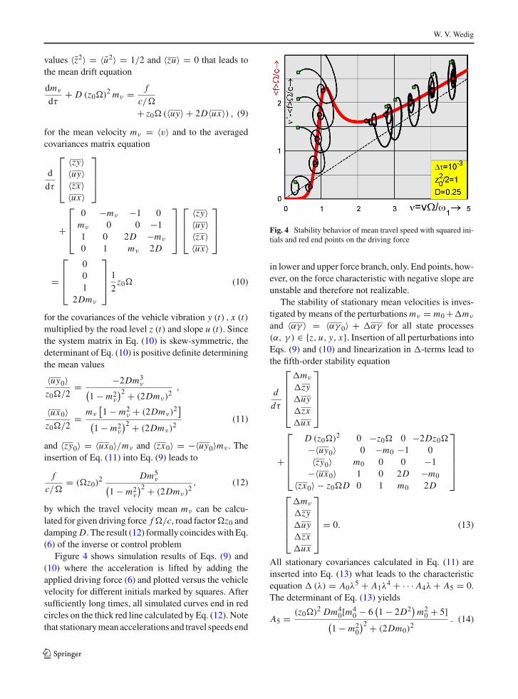
Figure 4 shows simulation results of Eqs. (9) and(10) where the acceleration is lifted by adding theapplied driving force (6) and plotted versus the vehiclevelocity for different initials marked by squares. Aftersufficiently long times, all simulated curves end in redcircles on the thick red line calculated by Eq. (12). Notethat stationarymean accelerations and travel speeds end
Fig. 4 Stability behavior of mean travel speed with squared ini-tials and red end points on the driving force
in lower and upper force branch, only. End points, how-ever, on the force characteristic with negative slope areunstable and therefore not realizable.
The stability of stationary mean velocities is inves-tigated by means of the perturbationsmν = m0+mν
and 〈αγ 〉 = 〈αγ 0〉 + αγ for all state processes(α, γ ) ∈ {z, u, y, x}. Insertion of all perturbations intoEqs. (9) and (10) and linearization in -terms lead tothe fifth-order stability equation
All stationary covariances calculated in Eq. (11) areinserted into Eq. (13) what leads to the characteristicequation (λ) = A0λ
5 + A1λ4 + · · · A4λ + A5 = 0.
The determinant of Eq. (13) yields
A5 = (z0�)2 Dm40[m4
0 − 6(1 − 2D2
)m2
0 + 5](1 − m2
0
)2 + (2Dm0)2
. (14)
123
Turbulent travel speeds in nonlinear vehicle dynamics
According to theHurwitzCriterion, A5 < 0 determinesdivergence and gives the boundaries of monotonousinstability. The new instability condition A5 < 0 deter-mined by Eq. (14) coincides with the negative slope ofthe driving force calculable by differentiating Eq. (12)with respect to the mean travel speed mν . The coinci-dence of both, negative slope and instability in mean,is plausible and physically explainable: A perturbationof stable speed into the negative direction on the leftside of the dynamic equilibrium generates accelerationsince the applied force is bigger than that one of thenew driving force of the perturbed speed. The vehi-cle, however, is braked if the speed perturbation goesinto positive speed direction on the right side of thedynamical equilibrium since then the driving force issmaller than that one necessary to maintain the per-turbed dynamic equilibrium. Vice versa, driving forceswith negative slope lead tomonotonous instability withthe effect that speed leaves the unstable branch of thedriving force, applied.
4 Stabilized integration by means of polarcoordinates
For constant speeds, the road equations (5) possesstwo eigenvalues with vanishing real parts what causesnumerical instability in integration routines. The result-ing drift is avoided by means of the polar coordinates
z = r cosϕ u = r sinϕ, (15)
The insertion of the coordinates (15) into the dimen-sionless forms dz = νudτ and du = −ν zdτ of the roadequations (5) gives the transformed road equations
dr = 0, r = 1, dϕ = −νdτ. (16)
where the related polar radius is integrated to r = 1 bywhich drift is eliminated and integration is stabilized.
Equations (15) and (16) are inserted into Eq. (7) thatgives the new covariance matrix equation
−νd
dϕ
⎡⎢⎢⎣
zyuyzxux
⎤⎥⎥⎦ +
⎡⎢⎢⎣
0 −ν −1 0ν 0 0 −110
01
2D −ν
ν 2D
⎤⎥⎥⎦
⎡⎢⎢⎣
zyuyzxux
⎤⎥⎥⎦
= z0�
2
⎡⎢⎢⎣
00
1 + cos2ϕ + 2Dνsin2ϕsin2ϕ + 2Dν (1 − cos2ϕ)
⎤⎥⎥⎦ . (17)
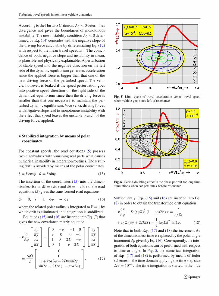
Fig. 5 Limit cycle of travel acceleration versus travel speedwhen vehicle gets stuck left of resonance
Fig. 6 Period-doubling effect in the phase portrait for long timesimulations when car gets stuck before resonance
Subsequently, Eqs. (15) and (16) are inserted into Eq.(8) in order to obtain the transformed drift equation
− νdν
dϕ+ D (z0�)2 (1 − cos2ϕ) ν = f
c/�
+ z0�(uy + 2Dux) − 1
2(z0�)2 sin2ϕ. (18)
Note that in both Eqs. (17) and (18) the increment dτ
of the dimensionless time is replaced by the polar angleincrement dϕ given byEq. (16). Consequently, the inte-gration of both equations can be performedwith respectto time or angle. In Fig. 5, the numerical integrationof Eqs. (17) and (18) is performed by means of Eulerschemes in the time domain applying the time step sizeτ = 10−4. The time integration is started in the blue
123
W. V. Wedig
square inside the limit cycle and ends in the yellow-black limit cycle around the yellow triangle on the driv-ing force calculated by Eq. (6). The transient behaviorfrom starting point up to the stationary limit cycle ismarked by a blue dashed line. The applied road factorand driving force are z0� = 0.7 and f �/c = 0.3,respectively. In addition, Fig. 5 shows results of a sec-ond simulation marked by a dashed green line whichrepresents themoving average of the simulation results.This line starts in the green square outside the limitcycle and ends in the yellow triangle on the drivingforce calculated byEq. (12).Moving average results arealready shown in Fig. 4 where the averaged equations(9) and (10) are solved, numerically. Both curves, theblack one in Fig. 4 and the green in Fig. 5, are slightlydifferent because the order of averaging and integra-tion is reversed in both figures. Finally, Fig. 6 showsthe period-doubling effect obtained for the parametersz0� = 0.9, f �/c = 0.6 and D = 0.2. Similar period-doubling effects are obtained when the travel velocityis plotted against the vibration velocity. The double-periodic limit cycle in Fig. 6 degenerates to the one-periodic limit cycle already shown in Fig. 5 when theroad factor z0� and the driving force f �/c are decreas-ing.
For analytical investigations, Eqs. (17) and (18) aresolved by means of the Fourier expansions
ν =j=+∞∑j=−∞
ν jexp ( j2ϕ) ,
�k =j=+∞∑j=−∞
�κjexp ( j2ϕ) , (19)
where �k is the vector of the covariances (zy, uy, zx, uz).The insertion of the two Fourier series (19) into the driftequation (18) and covariances equation (17) gives thetwo first equations of expansion
D (z0�)2 ν0 = f
c/�+ z0�
(uy0 + 2Dux0
),
(A + ν0B) �κ0 = z0�( �p/2 + D�qν0),
where the vectors �p and �q are determined by the right-hand side of Eq. (17) and the matrices A and B by itsleft-hand side. Both equations lead to the same velocitymean already calculated by averaging in Eq. (12) whenhigher terms of the Fourier expansion are neglected.
Summarizing it is noted that the longitudinal roadvehicle problem is solved according to the theory ofDA
equations by eliminating the infinitely growing vehi-cle motion coordinate. This is possible when the geo-metrical road equations are replaced by means of cor-responding dynamical ones. The calculated stationarysolutions are evaluated in phase portraits plotting thehorizontal acceleration versus the travel velocity. Thenumerical simulations show stable limit cycles beforeand after the resonance velocity, respectively. The mid-dle limit cycles on negative slopes of the applied driv-ing force are unstable and only detectable by means ofanalytical methods, e.g., by means of nonlinear Fourierexpansions. For increasing driving forces needed forgrowing road factor, the one periodic limit cycle bifur-cates into a double periodic one. For further growingdriving forces, the limit cycles become one periodic,again.
5 Random road profiles in space and time
In order to characterize wave length L = 2π/w andway frequency w of level and slope of stochastic roadprocesses, measurements [14] of one-dimensional pro-files are evaluated bymeans of power spectral densities[15–17] plotted versus the road frequencyw in double-logarithm scales. Random processes of road profilesare generated, e.g., by means of white way noise W
′s
with intensity σ applied to the oscillator equation
Z′′s + 2δ�Z
′s + �2Zs
= �σW′s, E
(W
′sW
′t
)= δ (s − t) , (20)
where δ > 0 denotes the bandwidth of the road processand the parameter � denotes its center frequency. Allprocesses in Eq. (20) are written in capital letters asset functions in dependence on the way coordinate s.Dashes denote derivatives with respect to s The inputterm in Eq. (20) is delta-correlated with zero mean. It isuniformly distributed in the frequency range [18] withthe power spectrum S(w) = 1.
The Fourier transform of Eq. (20) multiplied by itsconjugate version gives the road power spectrum [19]
Sz (w) = (�σ)2(�2 − w2
)2 + (2δ�w)2,
for |w| < ∞. (21)
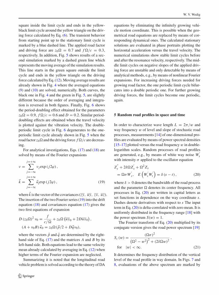
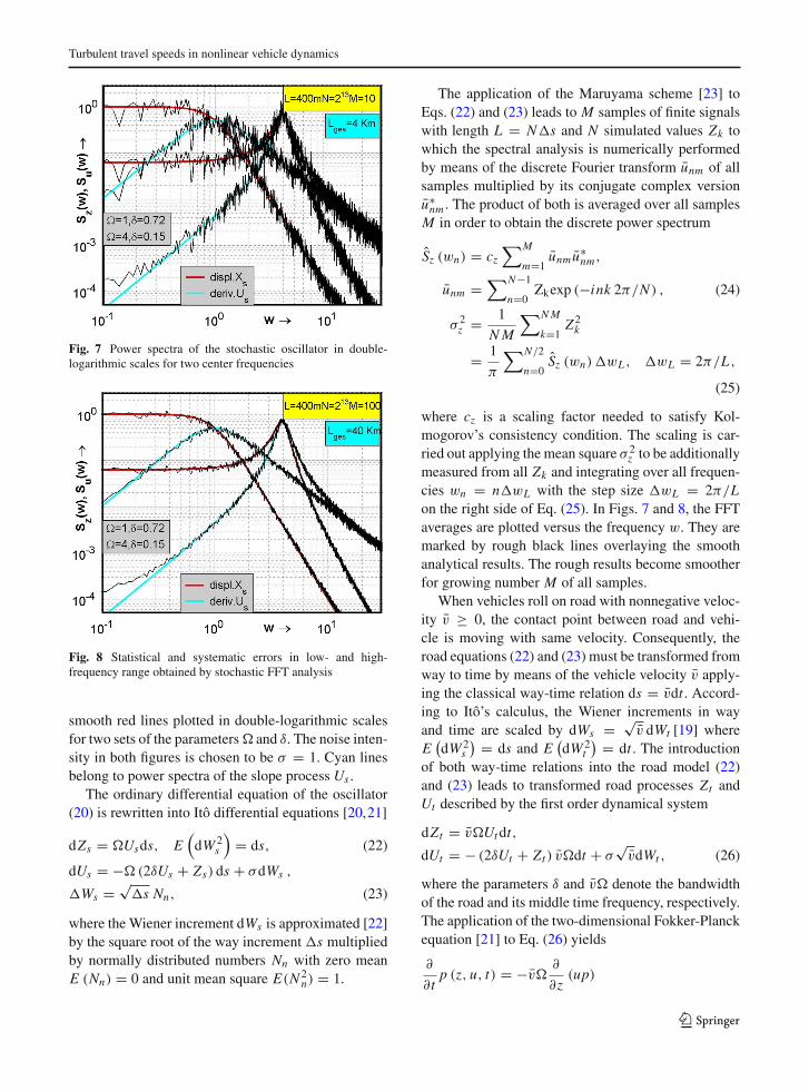
It determines the frequency distribution of the verticallevel of the road profile in way domain. In Figs. 7 and8, evaluations of the above spectrum are marked by
123
Turbulent travel speeds in nonlinear vehicle dynamics
Fig. 7 Power spectra of the stochastic oscillator in double-logarithmic scales for two center frequencies
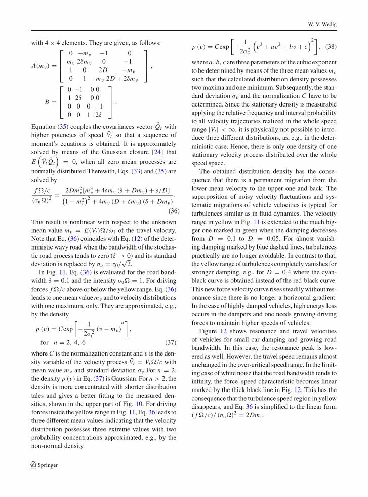
Fig. 8 Statistical and systematic errors in low- and high-frequency range obtained by stochastic FFT analysis
smooth red lines plotted in double-logarithmic scalesfor two sets of the parameters� and δ. The noise inten-sity in both figures is chosen to be σ = 1. Cyan linesbelong to power spectra of the slope process Us .
The ordinary differential equation of the oscillator(20) is rewritten into Itô differential equations [20,21]
dZs = �Usds, E(dW 2
s
)= ds, (22)
dUs = −�(2δUs + Zs) ds + σdWs ,
Ws = √s Nn, (23)
where the Wiener increment dWs is approximated [22]by the square root of the way increment s multipliedby normally distributed numbers Nn with zero meanE (Nn) = 0 and unit mean square E(N 2
n) = 1.
The application of the Maruyama scheme [23] toEqs. (22) and (23) leads to M samples of finite signalswith length L = Ns and N simulated values Zk towhich the spectral analysis is numerically performedby means of the discrete Fourier transform unm of allsamples multiplied by its conjugate complex versionu∗nm . The product of both is averaged over all samplesM in order to obtain the discrete power spectrum
Sz (wn) = cz∑M
m=1unmu
∗nm,
unm =∑N−1
n=0Zkexp (−ink 2π/N ) , (24)
σ 2z = 1
NM
∑NM
k=1Z2k
= 1
π
∑N/2
n=0Sz (wn)wL , wL = 2π/L ,
(25)
where cz is a scaling factor needed to satisfy Kol-mogorov’s consistency condition. The scaling is car-ried out applying the mean square σ 2
z to be additionallymeasured from all Zk and integrating over all frequen-cies wn = nwL with the step size wL = 2π/Lon the right side of Eq. (25). In Figs. 7 and 8, the FFTaverages are plotted versus the frequency w. They aremarked by rough black lines overlaying the smoothanalytical results. The rough results become smootherfor growing number M of all samples.
When vehicles roll on road with nonnegative veloc-ity v ≥ 0, the contact point between road and vehi-cle is moving with same velocity. Consequently, theroad equations (22) and (23) must be transformed fromway to time by means of the vehicle velocity v apply-ing the classical way-time relation ds = vdt . Accord-ing to Itô’s calculus, the Wiener increments in wayand time are scaled by dWs = √
v dWt [19] whereE
(dW 2
s
) = ds and E(dW 2
t
) = dt . The introductionof both way-time relations into the road model (22)and (23) leads to transformed road processes Zt andUt described by the first order dynamical system
dZt = v�Utdt,
dUt = − (2δUt + Zt ) v�dt + σ√
vdWt , (26)
where the parameters δ and v� denote the bandwidthof the road and its middle time frequency, respectively.The application of the two-dimensional Fokker-Planckequation [21] to Eq. (26) yields
∂
∂tp (z, u, t) = −v�
∂
∂z(up)
123
W. V. Wedig
+ v�∂
∂u[(2δu + z) p] + v
σ 2
2
∂2 p
∂u2.
This equation determines the joint density distributionof the two road processes in dependence on time. Inthe stationary case ∂p/∂t = 0, the velocity v dropsout with the consequence that the stationary densityp(zu) is independent on velocity. Consequently, theroad model (26) is applicable for all velocities v ≥0. This is exactly the same situation as, e.g., in thedeterministic casewhere the amplitude of the harmonicwave road remains unchanged when the vehicle speedsup or slows down.
6 Quarter car models rolling on random roadsurfaces
Quarter car models on random road are excited to ver-tical vibrations described by the equation of motion
Yt + 2Dω1(Yt − Zt
)
+ω21 (Yt − Zt ) = 0, (Yt = ω1Xt ) , (27)
where 2Dω1 = b/m determines the car damping andω1 is the natural frequency of the vertical vibrations,given by ω2
1 = c/m . In a first investigation, the veloc-ity v of the vehicle is assumed to be constant withthe consequence that the road vehicle system (26) and(27) becomes linear and can be solved, e.g., by meansof classical spectral methods [24]. Subsequently, theobtained car spectra are integrated over all spectral fre-quencies in order to calculate all mean squares andcovariances needed in the drift equation
Vt = [2Dω21(Y t − Zt ) + ω2
1 (Yt − Zt )] �Ut + Ft/m.
(28)
In the special case Vt = 0, the expectation E (Ft ) ofthe driving force is subsequently calculated to the form
E(Ft)
c�σ2u= 2D
ν2[ν3 + 4δν (δ + Dν) + δ/D
](1 − ν2
)2 + 4ν (D + δν) (δ + Dν),
(29)
where σz = σu are the standard deviations of the roadlevel and slope process. Both standard deviations arecalculable to σu = σ/
√4δ� by means of the linear
filter equations, noted in Eq. (26).In Fig. 9, the expected value (29) is plotted by a
red line versus the related car velocity ν = v�/ω1
for the road intensity �σ 2 = 1, the damping mea-sure D = 0.15 and the bandwidth δ = 0.3. The
Fig. 9 Force distributions simulated for constant speed and plot-ted together with the red force mean
mean force is overlaid by green circles of measuredvalues obtained by means of numerical simulationsapplying the Maruyama scheme with the step sizeτ = ω1t = 0.001 for N = 107 samples. Addi-tionally, Fig. 9 shows probability distributions p ( f )of the related driving process Ft�/c marked by bluelines and plotted for four speeds of the vehicle. Theobtained densities have the exponential form of Gaus-sian product processes with extremely wide distribu-tions indicating that the assumption of constant speedis physically not realizable.
Hence, it is more realistic to investigate the inverseproblem that the velocity is fluctuating meanwhile thedriving force is assumed to be constant or given byany characteristic depending on speed. This dynamicproblem is numerically investigated by means of thenonlinear first-order system
dYτ = Xτdτ,
d Xτ = − [2D
(Xτ − Vτ Uτ
) + Yτ − Zτ
]dτ, (30)
d Zτ = Vτ Uτdτ,
dUτ = − [2δ
∣∣Vτ
∣∣ Uτ + Vτ Zτ
]dτ+2
√δ∣∣Vτ
∣∣ dWτ
(31)
dVτ = (�σz)2 [2D
(Xτ−Vτ Uτ
)+Yτ−Zτ
]Uτdτ
+ Fτdτ, (32)
which is derived from Eq. (26), (27) and (28) introduc-ing the dimensionless state processes (Zt , Ut , Yt , Xt )
= σu(Zt , Ut , Yt , Xt
)and Ft = Ft�/c and Vt =
Vt�/c as well as the dimensionless time and noise bymeans of dτ = ω1dt and dWτ = √
ω1dWt , respec-
123
Turbulent travel speeds in nonlinear vehicle dynamics
Fig. 10 Velocity densities simulated for constant driving forcesoverlaid by red circles of mean speeds
tively. Note that the road equation (31) is slightly mod-ified in comparison with Eq. (26) through the introduc-tion of the absolute value of the velocity in the exci-tation and damping term The latter don’t change thefrequency behavior of the road process. However, tak-ing the absolute velocity value is necessary in dampingand excitation in order to ensure existence and stabil-ity in road simulations if the vehicle drives backwardswhere negative velocity occurs
In Fig. 10, probability density distributions of thevehicle velocity are plotted for given driving forces.The densities are obtained by means of numerical sim-ulations performed with the time step τ = 0.01 andN = 108 samples. Red circles represent measuredmean values of the simulated velocity process. The blueline represents the backbone curve of the mean drivingforce calculated by Eq. (29). For strong over-criticaldriving forces as shown in the upper right of Fig. 10,the calculated speeds are narrowly distributed withone peak, only. For decreasing driving force, however,the velocity distribution becomes broader and bifur-cates into bi-modal probability density with two peakswhen the driving force approaches its critical valuef �/c = 1 where the vertical car vibrations becomeresonant. In this case, the global mean value is splitinto two separated mean values; i.e., the car velocityis fluctuating around two means. Simultaneously, thevelocity ismigrating from onemean to the next one andback again. For further decreasing driving forces intothe under-critical range, the velocity regains its originaldistribution with one peak and one mean, only.
7 Probability bifurcation into turbulent travelspeeds
The control problem, where the mean value of the driv-ing force is calculated in Eq. (29), is now inverted inorder to investigate the associated dynamic problem offluctuating speeds when the driving force is constant.For these purposes, the velocity Vt is centralized bymeans of Vt = Vt + E(Vt ), that leads to E
(Vt
) = 0.The insertion of the mean-free velocity into the driftequation (28) gives
d(Vt
) = ( f/m)dt + ω21�{2DXtUt
−2D(�/ω1)[Vt + E (Vt )
]U 2t
+ (Yt − Zt )Ut }dt.Taking into account that E (ZtUt ) = 0 in the station-ary case and that the velocity Vt is uncorrelated to theroad surface processes Zt andUt , the above differentialequation leads to the stationary mean equation
f �/c + 2DE (XtUt ) − 2DmvE(U 2t
)
+ E (YtUt ) = 0, (33)
where E(U 2t
) = σ 2u and the mean speed is intro-
duced bymv = E(Vt )�/ω1. The stationary drift equa-tion (33) coincides with Eq. (8) when the dimension-less processes
(Yt , Xt
) = �(Yt , Xt ) and(Zt , Ut
) =(ZtUt )/z0 are inserted. The covariances E (XtUt ) andE (YtUt ) in Eq. (33) are determined by the vector equa-tion
d( �Qt
)= ω1
[−A �Qt − �
ω1BVt �Qt + �Pt
]dt
+ σ
√Vt + E(Vt ) �StdWt , (34)
where �St = (0,Yt , 0, Xt )′is the perturbation vector
�Qt = (Yt Zt , YtUt , Xt Zt , XtUt )′is the system vector
with four covariances and �Pt (mv) is the driving vectorgiven by (0, 0, P3t , P4t )′ and the components
P3t = Z2t + 2D[Vt�/ω1 + mv]ZtUt ,
P4t = ZtUt + 2D[Vt�/ω1 + mv]U 2t .
The application of the expectation operator to Eq. (34)leads to the stationary covariances equation
A (mv) E( �Qt
)+ BE
(Vt �Qt
)�/ω1 = �Pt (mv) ,
with �Pt (mv) = σ 2u (0, 0, 1, 2Dmv) , (35)
where the driving vector is calculated by means ofE (ZtUt ) = 0 and E
(Z2t
) = E(U 2t
) = σ 2u . The sys-
tem matrices A and B in Eq. (35) are skew-symmetric
123
W. V. Wedig
with 4 × 4 elements. They are given, as follows:
A(mv) =
⎡⎢⎢⎣
0 −mv −1 0mv 2δmv 0 −110
01
2D −mv
mv 2D + 2δmv
⎤⎥⎥⎦ ,
B =
⎡⎢⎢⎣
0 −1 0 01 2δ 0 000
00
01
−12δ
⎤⎥⎥⎦ .
Equation (35) couples the covariances vector �Qt withhigher potencies of speed Vt so that a sequence ofmoment’s equations is obtained. It is approximatelysolved by means of the Gaussian closure [24] that
E(Vt �Qt
)= 0, when all zero mean processes are
normally distributed Therewith, Eqs. (33) and (35) aresolved by
f �/c
(σu�)2= 2Dm2
v[m3v + 4δmv (δ + Dmv) + δ/D](
1 − m2v
)2 + 4mv (D + δmv) (δ + Dmv).
(36)
This result is nonlinear with respect to the unknownmean value mv = E(Vt )�/ω1 of the travel velocity.Note that Eq. (36) coincides with Eq. (12) of the deter-ministic wavy road when the bandwidth of the stochas-tic road process tends to zero (δ → 0) and its standarddeviation is replaced by σu = z0/
√2.
In Fig. 11, Eq. (36) is evaluated for the road band-width δ = 0.1 and the intensity σu� = 1. For drivingforces f �/c above or below the yellow range, Eq. (36)leads to onemean valuemv and to velocity distributionswith one maximum, only. They are approximated, e.g.,by the density
p (v) = Cexp
[− 1
2σ 2v
(v − mν)n]
,
for n = 2, 4, 6 (37)
whereC is the normalization constant and v is the den-sity variable of the velocity process Vt = Vt�/c withmean value mν and standard deviation σv For n = 2,the density p (v) in Eq. (37) is Gaussian. For n > 2, thedensity is more concentrated with shorter distributiontales and gives a better fitting to the measured den-sities, shown in the upper part of Fig. 10. For drivingforces inside the yellow range in Fig. 11, Eq. 36 leads tothree different mean values indicating that the velocitydistribution possesses three extreme values with twoprobability concentrations approximated, e.g., by thenon-normal density
p (v) = Cexp
[− 1
2σ 2v
(v3 + av2 + bv + c
)2], (38)
wherea, b, c are three parameters of the cubic exponentto be determined bymeans of the three mean valuesmν
such that the calculated distribution density possessestwomaxima and oneminimum. Subsequently, the stan-dard deviation σv and the normalization C have to bedetermined. Since the stationary density is measurableapplying the relative frequency and interval probabilityto all velocity trajectories realized in the whole speedrange |Vt | < ∞, it is physically not possible to intro-duce three different distributions, as, e.g., in the deter-ministic case. Hence, there is only one density of onestationary velocity process distributed over the wholespeed space.
The obtained distribution density has the conse-quence that there is a permanent migration from thelower mean velocity to the upper one and back. Thesuperposition of noisy velocity fluctuations and sys-tematic migrations of vehicle velocities is typical forturbulences similar as in fluid dynamics. The velocityrange in yellow in Fig. 11 is extended to the much big-ger one marked in green when the damping decreasesfrom D = 0.1 to D = 0.05. For almost vanish-ing damping marked by blue dashed lines, turbulencespractically are no longer avoidable. In contrast to that,the yellow range of turbulences completely vanishes forstronger damping, e.g., for D = 0.4 where the cyan-black curve is obtained instead of the red-black curve.This new force velocity curve rises steadilywithout res-onance since there is no longer a horizontal gradient.In the case of highly damped vehicles, high energy lossoccurs in the dampers and one needs growing drivingforces to maintain higher speeds of vehicles.
Figure 12 shows resonance and travel velocitiesof vehicles for small car damping and growing roadbandwidth. In this case, the resonance peak is low-ered as well. However, the travel speed remains almostunchanged in the over-critical speed range. In the limit-ing case of white noise that the road bandwidth tends toinfinity, the force–speed characteristic becomes linearmarked by the thick black line in Fig. 12. This has theconsequence that the turbulence speed region in yellowdisappears, and Eq. 36 is simplified to the linear form( f �/c)/ (σu�)2 = 2Dmv .
123
Turbulent travel speeds in nonlinear vehicle dynamics
Fig. 11 Resonance and traveling speeds of vehicles for smallroad bandwidth and decreasing car damping
Fig. 12 Resonance and traveling speed of vehicles for small cardamping and increasing road bandwidth
8 Conclusions
The paper investigates strong nonlinear systems in lon-gitudinal road vehicle dynamics. When the assumptionof constant speed is removed, nonlinearities are intro-duced by multiplicative state variables. They lead tothe effect that vehicle get stuck before resonance whendriving onwavy road surfaces. To overcome this block-ade, one has to speed up if the driving motor is strongenough.
Experiences on non-fixed wavy roads, e.g., dessertroads show that resonance speeds of vehicles are about40 km/h due to plastic deformations by heavy vehi-cles of road maintenance. Turbulences are avoidedby speeding up to over-critical speeds or by increas-
ing the car damping. Both leads to stronger drivingforces which are necessary to balance the energy lossin dampers.
Bifurcations in probability are explained by the factthat stationary density distributions of interest possessthree extreme values: two maxima and one minimumindicating that solution trajectories are seldom in theminimum and often in the maxima with a permanentchange between both. This is completely different tothe linear case where the trajectories are Gaussian anddistributed with one maximum, only.
Acknowledgements Open Access funding provided by Pro-jekt DEAL.
Compliance with ethical standards
Conflict of interest The author declares that he has no conflictof interest.
Open Access This article is licensed under a Creative Com-mons Attribution 4.0 International License, which permits use,sharing, adaptation, distribution and reproduction in anymediumor format, as long as you give appropriate credit to the originalauthor(s) and the source, provide a link to the Creative Com-mons licence, and indicate if changes were made. The images orother third partymaterial in this article are included in the article’sCreative Commons licence, unless indicated otherwise in a creditline to thematerial. If material is not included in the article’s Cre-ative Commons licence and your intended use is not permitted bystatutory regulation or exceeds the permitted use, you will needto obtain permission directly from the copyright holder. To viewa copy of this licence, visit http://creativecommons.org/licenses/by/4.0/.
References
1. Wedig, W.V.: Jump phenomena in road-vehicle dynamics.Int. J. Dyn. Control 4, 21–28 (2016)
2. Wedig, W.V.: New resonances and velocity jumps in nonlin-ear road-vehicle dynamics. In: Hagedorn, P. (ed.) Proceed-ings of IUTAM Symposium on Analytical Methods in Non-linear Dynamics, Frankfurt, Germany, July 2015, ProcediaIUTAM, Elsevier, pp. 1–9. www.sciencedirect.com (2016)
abilistic Workshop, DresdenTUD Press, vol. 1, pp. 1–13(2017)
8. Wedig, W.V.: Velocity jumps in road-vehicle dynamics.In: 12th International Conference on Vibration Problems(ICOVP 2015), Procedia Engineering, vol. 144, pp. 1076–1085. www.sciencedirect.com (2016)
9. Ascher, U.M., Petzold, L.R.: Computer Methods for Ordi-naryDifferential equations andDifferential-Algebraic equa-tions. SIAM, Philadelphia (1998)
10. Sommerfeld, A.: Beiträge zum dynamischen Ausbau derFestigkeitslehre. Z. Ver. Deut. Ing. 46, 391–394 (1902)
11. Wedig, W.V.: Lyapunov exponents and rotation numbersin rotor- and vehicle dynamics. Proc. Eng. 199, 875–881(2017)
12. Drozdetskaya, O., Fidlin, A.: On the dynamic balancing ofa planetary moving rotor using a passive pendulum-typedevice. Proc. IUTAM 18, 126–135 (2016)
13. Fidlin, A., Drozdetskaya, O.: On the averaging in stronglydamped systems: the general approach and its application toasymptotic analysis of the Sommerfeld effect. Proc. IUTAM18, 43–52 (2016)
14. Braun, O.: Untersuchungen von Fahrbahnunebenheiten undAnwendungen der Ergebnisse, Diss. Universität Hannover(1969)
15. Doods, C.J., Robson, J.D.: The description of road surfaceroughness. J. Sound Vibr. 31, 175–183 (1973)
16. Sobczyk, K., MacVean, D., Robson, J.: Response to profile-imposed excitationwith randomlyvarying transversal veloc-ity. J. Sound Vibr. 52, 37–49 (1977)
17. Popp, K., Schiehlen, W.O.: Fahrdynamik. Teubner-Verlag,Germany (1993)
18. Ammon, D., Wedig, W.: The approximation and the gener-ation of stationary vector processes. Probabilistic Methodsin Applied Physics, Lecture Notes in Physics 451 (1995)
19. Wedig, W.V.: Dynamics of cars driving on stochastic roads.In: Spanos, P., Deodatis, G. (eds.) Computational Stochas-tic Mechanics CSM-4, pp. 647–654. Millpress, Rotterdam(2003)