Abstract This paper exploits variation in the mandated insurance coverage ofassisted reproductive technology (ART) across US states and over time to examinethe connection between increased access to ART and female marriage timing. SinceART increases the probability of pregnancy for older women of reproductive age,greater access to ART will make marriage delay less costly for younger single womenof reproductive age. Linear probability models are estimated to investigate the effectsof ART state insurance mandates on changes in marital status of women in differ-ent age groups using the 1977–2010 Current Population Survey. Results show thatgreater access to ART is associated with marital delay for white (but not for black)women: white women in states with an ART insurance mandate are significantly lesslikely to marry between the 20–24, 25–29, and 30–34 age ranges, but significantlymore likely to marry between the 30–34 and 35–39 age ranges.
Keywords Marriage · Economics of the family · Assisted reproductivetechnology · Infertility · Insurance mandates
JEL Classifications I18 · J12 · J13
AbbreviationsART Assisted reproductive technologyIVF In vitro fertilizationCDC Centers for Disease Control and PreventionGIFT Gamete intrafallopian transfer
Responsible editor: Erdal Tekin
J. Abramowitz (�)U.S. Census Bureau, 4600 Silver Hill Road, Washington, DC 20233, USAe-mail: [email protected]: https://sites.google.com/site/joelleabramowitz/
ZIFT Zygote intrafallopian transferHMO Health maintenance organizationCPS Current Population SurveyIPUMS Integrated Public Use Microdata Series
1 Introduction
The past several decades have seen far-reaching changes in the lives of women:women have been marrying and having children later or forgoing marriage and moth-erhood altogether, and the number of women in college and professional schoolshas greatly increased as has the number of women pursuing careers. Over the sameperiod, there have been significant developments in the technology of conceptionand contraception, affording women more control over their fertility. While severalpapers have addressed the question of whether contraceptive technology has influ-enced women’s choices beyond the scope of their birth timing, this paper examinesthe connection between affordability of assisted reproductive technology (ART) andfemale marriage timing.
Goldin and Katz (2002) and Bailey (2006) examine whether the availability of acontraceptive technology, the birth control pill, impacted women’s choices beyondthe scope of their birth timing. Goldin and Katz (2002) show that greater access tothe pill was associated with being less likely to marry before age 23, more likely to beemployed in professional occupations, more likely to never marry, and less likely tobe divorced. Bailey (2006) finds that early legal access to the pill was associated witha reduced likelihood of a first birth before age 22, an increased number of womenin the paid labor force, and an increase in their number of annual hours worked. Theresults of these papers suggest that a fertility technology can impact women’s choicesabout more than only when to get pregnant.
While the above papers examine the effects of the diffusion of a contraceptivetechnology, this paper builds on the above literature by investigating the effectsof a development in the technology of conception: ART. ART consists of medicaltechnologies that help women and couples with fertility problems conceive a childusing such methods as in vitro fertilization (IVF). While several papers examinehow the mandates have affected the use of infertility treatment (Jain et al. 2002;Bitler and Schmidt 2006; Bundorf et al. 2007; Bitler and Schmidt 2012) and othersexamine the effects of the mandates on birth outcomes (Schmidt 2007; Bitler 2008;Buckles 2012; Ohinata 2011), this paper investigates whether ART has in factaffected more than only women’s infertility treatment use or birth timing; in partic-ular, this paper will focus on whether affordability of this technology has affectedwomen’s decisions about when to marry. The introduction of ART could result inchanges in women’s timing of marriage by making it less costly to delay pursuingmarriage in order to invest in education and a career or search longer for a spouse.
However, identifying whether advances in reproductive technology have in factaffected women’s life choices is not straightforward. Over the same period whenthese technologies became available, women achieved greater educational and careeropportunities, and it is these developments that have in turn increased the demand
Effect of affordability of ART on women’s marriage timing 605
for delayed fertility and driven developments in the field of reproductive technology.Since the advances in women’s education, career, and reproductive technology werecodetermined, an analysis must be careful to identify the effects of each of theseforces separately. In their analysis of the effects of availability of the birth controlpill, Goldin and Katz (2002) and Bailey (2006) exploit cross-state variation in the ageof majority and hence legal access to the birth control pill. To identify the effects ofART separately from other forces affecting women’s marriage decisions, this paperexploits exogenous state variation in mandated insurance coverage of ART.
This paper uses variation in the mandated insurance coverage of ART to developseveral empirical specifications to examine whether greater affordability of ARTis associated with changes in women’s marriage timing. The empirical analysisestimates the likelihood that women of different ages with and without mandatedinsurance coverage of ART have ever been married in order to compute marriagerates between age groups, the differences in the likelihoods of having ever been mar-ried between one age group and the next. By examining marriage rates between agegroups, the analysis can be used to determine whether greater affordability of ARTis associated with changes in women’s marriage timing.
The results of the empirical analysis suggest that the mandates are associated witha pattern of marriage delay. Across all ages, the mandates appear to be associatedwith a lower likelihood of ever marrying: significant negative effects of the man-dates on the probability of ever having married are found for women ages 20–49 forthe full sample and for whites. However, it appears that the effects of the mandatesvary greatly for women of different ages and are consistent with a pattern of mar-riage delay: estimating the effects of the mandates by age group suggests that forwhite women, the mandates are associated with a significantly lower probability ofmarrying over the 20–24, 25–29, and 30–34 age ranges and a significantly higherprobability of marrying over the 30–34 and 35–39 age ranges. None of the mandateestimates were significant for blacks.
The rest of the paper is organized as follows. The next sections provide some back-ground on women’s age at first marriage as well as infertility and the ART insurancemandates. The following section develops a theoretical framework for understandinghow ART might affect women’s marriage timing decisions. The next sections outlinethe empirical specifications, present the data used in the analysis, and show results ofthe analysis. The last section concludes this study.
2 Changes in marriage
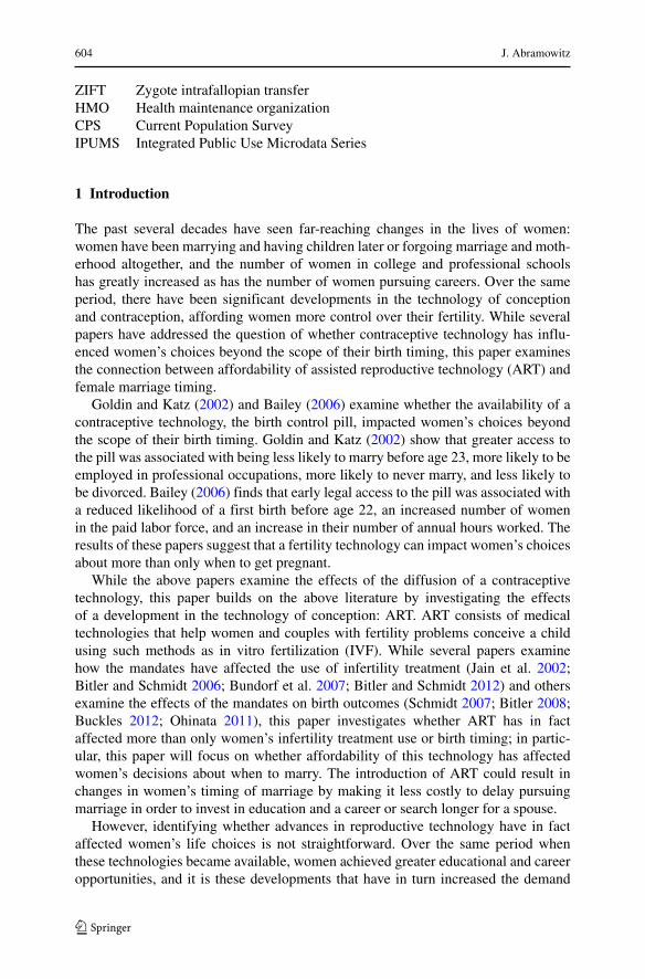
Over the past several decades, there have been considerable changes in women’spropensity to marry and timing of marriage. As shown in Fig. 1, over 1977 to 2010, atall ages, the proportion of women ever married has decreased. While the likelihood toever marry has also decreased, the likelihood of marrying at younger ages has fallendramatically: in 1977, over 50 % of women ages 20–24 had married, but by 2010,the proportion fell to little more than 20 %. There has been extensive discussion inthe economics literature as well as in the social sciences literature generally aboutthe drivers of this change in marriage behavior as well as its consequences.
606 J. Abramowitz
.2.4
.6.8
1
20-24 25-29 30-34 35-39 40-44 45-49Age Group
1977 19902000 2010
Fig. 1 Proportion women ever married by age group (1977, 1990, 2000, 2010). Over 1977 to 2010, at allages, the proportion of women ever married has decreased. While the likelihood of ever having marriedby older ages has decreased, the likelihood of ever having married at younger ages has fallen dramatically.Source: Integrated Public Use Microdata Series, Current Population Survey March Supplements, 1977,1990, 2000, 2010 from King et al. (2010)
From an economic perspective, understanding individuals’ decisions aboutwhether and when to marry is valuable since marriage can affect their work, fam-ily, and other life decisions and because it is useful to think of the marriage marketitself as analogous to the labor market. While the institutional theory of marriage(Goode 1964; Modell 1985; Thornton 1989) would suggest that marriage behaviormight not be influenced by changes in the costs and benefits of marriage, using theframework pioneered by Becker (1973, 1974, 1981), it would be expected that deci-sions about marriage should respond to changes in the costs and benefits of marriage.This paper will examine whether changes in the affordability of ART have affectedwomen’s likelihood of marrying at different ages. However, over the same periodthat ART became more available and affordable, changes in many other factors havebeen found to contribute to changes in women’s marriage behavior as well.
One of the most important changes in the lives of women has been the significantlyexpanded labor market opportunities for women. Goldin (2006) identifies key fac-tors in women’s changing economic roles over the last century: the increased relativedemand for female office workers, the growth of educational institutions at the sec-ondary level, changes in household production technology, and institutional changesmaking part-time work readily available and removing barriers to the employment ofmarried women. Given the vast changes in women’s economic lives, it follows thatthere could be effects on women’s personal lives, and the paper suggests the connec-tion between women’s greater labor market opportunities and a later age at first mar-riage for women pursuing higher education beginning in the 1970s. Blau et al. (2000)
Effect of affordability of ART on women’s marriage timing 607
also find that women’s as well as men’s decisions to marry were responsive totheir own labor market opportunities: using 1970, 1980, and 1990 data, they findthat women delay marriage when their own opportunities in the labor marketimprove or when men’s opportunities in the labor market worsen. This suggests thatwomen’s decisions about marriage are increasingly driven by greater labor marketopportunities.
In addition to changes in the economic roles of women, changes in general eco-nomic conditions have also been found to contribute to women’s marital delay.Inequality has increased greatly over recent decades, and if women search longerfor a spouse when there is higher male wage inequality, this could be an importantfactor contributing to delayed marriage. Loughran (2002) and Gould and Paserman(2003) examine the connection between increasing male wage inequality and declin-ing female marriage rates within cities and establish a causal connection between theformer and the latter.
Over the same period, changes in social constructs related to marriage have alsohad the potential to impact women’s marriage decisions. Prevalent attitudes havebecome more tolerant of premarital sex, cohabitation, and out-of-wedlock childbear-ing resulting in less of a social cost of remaining unmarried. Bumpass et al. (1991)examine the incidence of cohabitation in light of declining marriage rates and findthat individuals are increasingly opting for cohabitation rather than marriage.
At the same time, there have been significant legal and technological develop-ments related to birth timing. Changes in abortion laws made abortion much morewidely available, and concurrently, a number of developments in the technology ofconception and contraception afforded women more control over their birth timing.Akerlof et al. (1996) discuss how the legalization of abortion and the increased avail-ability of contraception for unmarried women led to a decline in shotgun marriages.Myers (2012) examines the effects of state policies related to access to oral contra-ception and to abortion on young women’s probabilities of entering into marriageand parenthood at a young age and finds a significant negative effect of abortion butno significant effect of oral contraception, while Goldin and Katz (2002) provide evi-dence that the availability of oral contraception has caused women to delay marriageand Bailey (2006) shows that early legal access to oral contraceptives is associatedwith women’s delay of childbearing and greater labor force participation.
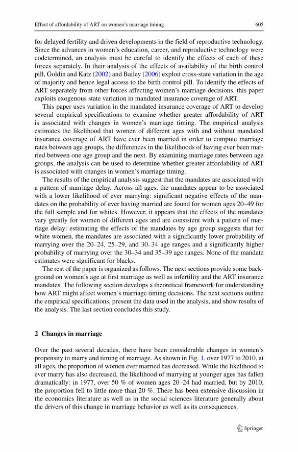
This paper considers ART as a driver of changes in women’s marriage timingusing variation in the mandated insurance coverage of ART across US states and overtime. As can be seen in Fig. 2, in the premandate period, differences in marriage rateswere evident at younger ages but converged for women in their mid-20s and older. Inthe postmandate period, differences in marriage rates increased for women from theirlate teens through their early 30s and only then began to converge for women at olderages.1 These differential trends in the proportion ever married at each age before andafter mandate implementation suggests that the mandates could be associated withdelayed marriage, but it is necessary to further examine this question controlling forother factors that could be influencing marriage rates across states and over time.
1The pre-mandate period includes 1977, and the post-mandate period includes 2001–2010.
608 J. Abramowitz
0.2
.4.6
.81
20 30 40 50Age
No Mandate - Pre No Mandate - PostMandate - Pre Mandate - Post
Fig. 2 Proportion ever married by mandate status pre- and posttreatment. In the premandate period, differ-ences in marriage rates were evident at younger ages but converged from the mid-20s. In the postmandateperiod, differences in marriage rates increased through the early 30s and only then began to converge.Source: Integrated Public Use Microdata Series, Current Population Survey March Supplements, 1977,1990, 2000, 2010 from King et al. (2010)
There have been many explanations for the increase in marriage delay of recentdecades. This paper continues to examine the propensity of women to delay marriageand considers access to infertility treatment in this regard. Further, the social, legal,and economic changes discussed above that make marriage delay less costly can onlybe effective if women believe they can delay their birth timing as well: in this way,ART may have facilitated the phenomena described above. By identifying systematicvariation in the availability of ART, the analysis can investigate the effect of ARTseparate from these co-determined factors.
3 ART and insurance mandates
Infertility is defined as the inability to conceive after a year of unprotected inter-course. While infertility treatments in general are defined as medical technologiesthat help women and couples with fertility problems conceive a child and can includea wide range of services from counseling and fertility testing to surgical procedures,the definition of ART used by the Centers for Disease Control and Prevention (CDC)includes all infertility treatments in which both eggs and sperm are handled. In 2002,11.9 % of women 15–44 years of age had ever received any infertility services, and1.1 % had undergone artificial insemination procedures. One of the most well-knownART procedures is IVF, whereby an egg is taken from a woman’s ovaries, fertilized,
Effect of affordability of ART on women’s marriage timing 609
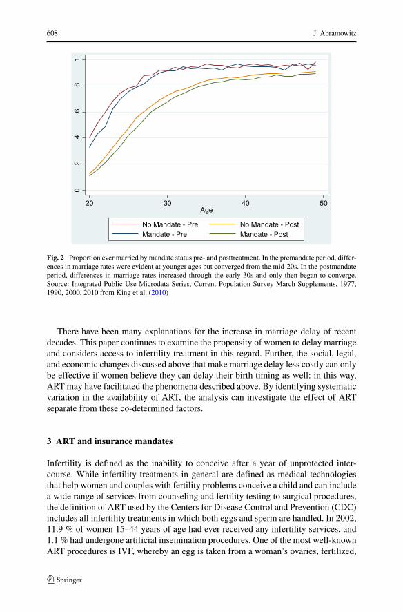
and then placed in her uterus. The first successful IVF procedure in the USA wasperformed in 1981, and since that time, ART procedures have become much moreeffective and widely used. Other related ART procedures include GIFT and ZIFT,but these procedures are much less commonly used as compared to IVF. By 2008,the CDC estimated that ART accounted for slightly more than 1 % of all US births.In 2008, 36.9 % of ART cycles using fresh non-donor eggs or embryos resulted inclinical pregnancies, and 81.2 % of these pregnancies resulted in live births. In 2008,71.2 % of women who had ART cycles using fresh non-donor eggs or embryos hadno previous births. Figure 3 shows the distribution of the users of ART using non-donor eggs or embryos by age. As can be seen in the figure, while some women useART with their own eggs or embryos during their 20s, the majority are at least intheir 30s, and nearly all women are younger than 45 (Centers for Disease Controland Prevention, American Society for Reproductive Medicine, Society for AssistedReproductive Technology 2010).
While the development of infertility treatments has benefitted many women, itmust be noted that many women are unable to use these treatments due to their highprices. Hormone therapy can cost between a few hundred and a few thousand dollars,and a single cycle of IVF can cost around $10,000 (Bitler and Schmidt 2012). Giventhat less than one-third of ART cycles using non-donor eggs or embryos result inlive births (Centers for Disease Control and Prevention, American Society for Repro-ductive Medicine, Society for Assisted Reproductive Technology 2010), it may take
-
1.00
2.00
3.00
4.00
5.00
6.00
7.00
8.00
9.00
<24 25 27 29 31 33 35 37 39 41 43 45 47 >48
Per
cen
t
Age (Years)
Fig. 3 Age distribution of women who had ART cycles using fresh non-donor Eggs or embryos, 2008.The figure shows the age distribution of the users of ART using non-donor eggs or embryos. While somewomen use ART with their own eggs or embryos during their 20s, the majority are at least in their 30s, andnearly all women are younger than 45. Source: (Centers for Disease Control and Prevention, AmericanSociety for Reproductive Medicine, Society for Assisted Reproductive Technology 2010), p. 28
610 J. Abramowitz
multiple cycles of ART to be successful, and the costs of procedures and medicationscan quickly become prohibitive.2
It would be ideal to examine how the introduction and availability of ART hasaffected the expectations and choices of women with regard to marriage at differentages. However, the introduction of ART followed a gradual process, and variationin its availability has certain endogenous drivers. As a result, this paper uses analternative and potentially exogenous source of variation affecting the use of ART:price.
While the prices of infertility treatment on their own do not vary in a systematicway, insurance coverage of ART does vary systematically by state. ART is gener-ally not covered by insurance unless firms are required by a state mandate to theiremployees with insurance plans that cover it. In total, 15 states currently mandateinsurance coverage for ART in some form. There could be some concern that stateswith mandates are fundamentally different from those that do not have mandates. Itshould be noted that the list of mandate states includes a very heterogeneous groupof states geographically, politically, and otherwise. Anecdotal evidence suggests thatstates’ adoption of the mandates often comes about due to idiosyncratic factors unre-lated to their residents’ considerations about delaying marriage and childbearing.The introduction of the ART insurance mandates was part of a greater trend in theimplementation of insurance mandates in the USA between the 1970s and 1990s.Lobbying in favor of the mandates has generally been at the national level and hasbeen led by RESOLVE, an organization promoting reproductive health and equalaccess to infertility treatment. The argument for the mandates is that infertility is alife-altering disease and that individuals should be able to insure against infertilitylike they would other such conditions. It appears that a primary factor determin-ing whether a state implemented any particular mandate, including ART insurancemandates, was the state’s view toward mandates generally, rather than its residents’demand for the particular benefits mandated to be covered. This anecdotal evidencesuggests that interests in delaying marriage and childbearing did not drive state’sadoption of the mandates. To test for endogeneity of the implementation of the man-dates, in this analysis, a lead of the mandate variable interacted with age group wastested in the full empirical specifications, and it was not found to be significant.3
The states mandating insurance coverage of ART are Arkansas, California,Connecticut, Hawaii, Illinois, Louisiana, Maryland, Massachusetts, Montana, NewJersey, New York, Ohio, Rhode Island, Texas, and West Virginia. The enactment ofthe mandates began as early as 1977 in West Virginia and continued until as recentlyas 2001 in Louisiana and New Jersey. The mandates vary in whether they require thatinfertility treatment be covered if coverage is offered, known as a “mandate to cover”or only that a plan that includes infertility treatment be offered to firms offering insur-ance, known as a “mandate to offer.” In addition, some of the mandates only apply to
2Success rates are similar for ART cycles using fresh or frozen non-donor eggs or frozen donor eggs;success rates for ART cycles using frozen donor eggs are higher, but still, only less than one-half of ARTcycles using frozen donor eggs result in live births.3This follows Bitler and Schmidt (2012).
Effect of affordability of ART on women’s marriage timing 611
HMOs and some specifically mention that IVF be covered or be excluded from cov-erage. It is important to note that the mandates do not affect all residents of a stateas the Employee Retirement Income Security Act of 1974 designates that state insur-ance mandates only affect individuals insured through firms that purchase insurancefrom an outside provider. However, larger firms that self-insure have increasinglyprovided the mandated coverage (Acs et al. 1996; Jensen and Morrisey 1999). Forexample, according to King and Meyer (1997), half of all workers in Illinois wereaffected by the Illinois mandate in 1993. While it might be a concern that benefitsare similar in firms in states that mandate relative to firms in states that do not man-date, Bitler and Schmidt (2012) note that this is not usually the case for infertilitytreatment, which is rarely covered in the absence of mandates.
Table 1 provides a list of the states with mandates currently in place as well as thedate the mandates were enacted and relevant details. It is important to note that whilethe mandates cover only 15 states, they affect a relatively large share of births in theUSA. States with mandates comprised over 47 % of births in the USA in 2008.4
While this paper explores whether the insurance mandates have influencedwomen’s marriage behavior in response to changed expectations about their futurefertility, it is first useful to ascertain whether the mandates have actually resulted inincreased use of infertility treatments. Bundorf et al. (2007) find that use of infer-tility treatments is significantly greater in states adopting comprehensive versionsof the mandates and that while greater utilization had little impact on the numberof deliveries, mandated coverage was associated with a relatively large increase inthe probability of a multiple birth. Buckles (2012) also finds that strong mandate-to-cover laws are associated with an increase in multiple birth rates for married women,white women, and for women with a college degree. Hamilton and McManus (2012)find that comprehensive mandates result in large increases in access to treatment aswell as significantly less aggressive treatment.5 Bitler and Schmidt (2012) examinewhether the mandates affect ART utilization for older, highly educated women andfind that they have a large and significant effect for this subgroup. All of these paperssuggest that the mandates are indeed associated with increased use of ART and thatthis increased utilization is associated with differential birth outcomes. However,Bitler and Schmidt (2006) find no evidence that the mandates ameliorate racial, eth-nic, and education disparities in the use of infertility treatment suggesting that theremay be differential effects of the mandates on these groups. Since it appears that themandates are affecting the choices of the users of ART, this paper asks whether theeffects of the mandates permeate beyond only the current users of ART to affect themarriage behavior of women who may or may not ever be consumers of ART. Notingthe racial, ethnic, and education disparities in the use of ART, this paper will exam-
4Centers for Disease Control and Prevention, National Center for Health Statistics, VitalStats (2011).5In contrast to Bundorf et al. (2007) and Buckles (2012), Hamilton and McManus (2012) find that the man-dates are actually associated with a decrease in the percentage of pregnancies with three or more fetuses.Their contradictory results with respect to the impact of the mandates on aggressiveness of treatment andmultiple births could be due to alternative samples and econometric techniques accounting for changes inthe population using ART versus changes in procedures and outcomes for the population that would havereceived treatment without the mandates.
612 J. Abramowitz
Table 1 States with mandated infertility insurance. Source: American Society for Reproductive Medicine(2011), RESOLVE (2011), Bitler and Schmidt (2012)
State Year Law Enacted Mandate to cover Mandate to offer IVF coverage IVF only
Arkansas 1987 X X
California 1989 X
Connecticut 1989 X X
Hawaii 1987 X X
Illinois 1991 X X
Louisiana 2001 X
Maryland 1985 X X
Massachusetts 1987 X X
Montana 1987 X
New Jersey 2001 X X
New York 1990 X
Ohio 1990 X
Rhode Island 1989 X X
Texas 1987 X X
West Virginia 1977 X
Connecticut changed its mandate from a mandate to offer in its 1989 law to a mandate to cover in its 2005law. According to RESOLVE (2011) and as in Bitler and Schmidt (2012), Louisiana is considered to haveimplemented a mandate to cover beginning in 2001. According to the American Society for ReproductiveMedicine (2011) and as in Bitler and Schmidt (2012), West Virginia is considered to have implementeda mandate to cover beginning in 1977. As in Bitler and Schmidt (2012), New York is considered to haveimplemented a mandate to cover beginning in 1990
ine the effects of the mandates separately for the marriage behavior of women fromdifferent groups in order to identify any differential effects of the mandates in thisanalysis.
The economics literature has also begun to investigate if there are significanteffects of the mandates on larger populations of women, not just the users of ART.The previous literature has focused on examining women at older childbearing agesbecause they are more likely to be infertile and demand treatment and because theytend to be privately insured at high rates. Several papers find that the mandates areassociated with changes in birth rates. Schmidt (2007) uses Vital Statistics DetailNatality Data and Census population counts and finds that the mandates increasefirst birth rates for women over 35. Buckles (2005) uses Vital Statistics Detail Natal-ity Data to show that mandates that cover IVF are associated with a higher age atfirst birth. Bitler (2008) finds that the mandates are associated with an increase inthe probability of being a twin for children born to older mothers, an increase inthe twin delivery rate for older women, as well as negative effects on health-relatedcharacteristics for samples of twins and, to a lesser extent, singletons. Using thePanel Study of Income Dynamics, Ohinata (2011) finds results suggesting that themandates are associated with younger women delaying child bearing. Only a fewpapers have considered the effects of the mandates on outcomes not related to births.
Effect of affordability of ART on women’s marriage timing 613
Cohen and Chen (2011) find that the mandates are associated with increased adop-tion rates, and Appleton and Pollak (2011) put these adoption results in context.Buckles (2005) finds that mandating insurance coverage increases labor force par-ticipation for women under 35 and decreases participation for women over 35 whileincreasing their wages. Lahey (2012) finds that for older women of childbearing age,the mandates do not appear to affect wages, but are associated with a decrease in totallabor input.
This paper expands on this literature by considering the effects of increased afford-ability of ART on women’s marriage timing. While most of the aforementionedpapers focus primarily on examining the effects of the mandates on the users of ART,this paper considers the effects of the mandates on all women through their expec-tations of their future fertility regardless of whether they will ever actually use ART.In addition, this paper adds to the existing literature by examining the effects of themandates on marriage outcomes rather than fertility or labor market outcomes. Toidentify the potential effects of the mandates, the paper next develops a theoreticalframework for understanding how greater affordability of ART could affect women’smarriage timing.
4 Theoretical framework
Lowering the price of ART through insurance mandates provides for greater accessto ART, making it available for many women. To develop a framework for under-standing how greater affordability of ART could affect women’s decisions aboutmarriage, this section presents a theoretical model building on the one presented inGoldin and Katz (2002) for identifying how the diffusion of the birth control pillcould have affected professional career investments and the timing of marriage byyoung women.
I consider a three-period model with no discounting where there are an equalnumber of men and women. For simplicity, I assume that it is only possible tohave children within marriage and marriage and childbearing take place in the sameperiod. To a marriage, each man brings Hi , a husband contribution; Fi , a fathercontribution; and Yi , an income contribution; and each woman brings Wj , a wife con-tribution; and Mj , a mother contribution. If a woman invests in a career in the firstand second periods, she also brings αj , a career return treated as a household publicgood for each period of investment. The distributions of H, F, Y, W, M, and α areknown by all participants, and each individual’s attributes are perfectly observable.Assume that Fi and Mj only contribute to the payoff of the marriage if it results inchildren, determined by the woman’s probability of pregnancy, π . π is assumed tobe the same for all women, and is initially π0 in the first and second periods, butdeclines between the second and third periods by �π . I assume that a marriage canonly produce biological children.
As in Goldin and Katz, I assume that a woman’s career investment in the firstperiod is only possible if she delays marriage to the second period, which reducesutility by λ, the “impatience factor” for each partner, representing the utility lostfrom abstinence as well as from foregone home production. Goldin and Katz showed
614 J. Abramowitz
how all women with αj > λ would invest in careers and delay marriage untilthe second period while all others would marry in the first period. They thenshowed how the availability of the pill could reduce λ and shift down the cut-off point in the α distribution, leading more women to delay marriage and pursuecareers.
I further assume that a woman’s career investment in the second period is only pos-sible if she delays considering marriage to the third period. For simplicity, I assumethe payoff to continued career investment is again αj and utility is again reduced byλ, but now, I also assume that utility is further reduced by �π ∗ (Fi +Mi), the “tick-ing clock factor” for each partner, representing the utility lost from being less likelyto have children as a result of a lower probability of pregnancy.
The payoff to a marriage between a man i and a woman j is determined by eachpartner’s contributions as well as the probability they have children and start a family.If a man and woman marry in the first period, the payoff is: π0 ∗ (Fi + Mi) + Hi +Yi + Wj .
If the woman invests in a career in the first period and marriage is delayed until thesecond period, the payoff of the marriage is: π0∗(Fi + Mi) +Hi +Yi+Wj +αj −λ.
If the woman invests in a career in the first period and continues to invest in acareer in the second period so that marriage is delayed until the third period, thepayoff of the marriage is: (π0 − �π) ∗ (Fi + Mi) + Hi + Yi + Wj + 2αj − 2λ.
As in Goldin and Katz, if αj < λ, the woman considers marriage in the firstperiod, and if αj > λ, the woman invests in a career in the first period and doesnot consider marrying in the first period. If λ < αj < λ + �π ∗ (Fi + Mi), thewoman considers marrying in the second period and she does not continue to investin her career. If αj > λ + �π ∗ (Fi + Mi), then the woman further delays consid-ering marrying until the third period and continues to invest in a career in the secondperiod.
Unlike Goldin and Katz, I do not assume that all individuals marry. This modelassumes that individuals choose when to consider marrying, and then a man andwoman will choose to marry if the payoff to the marriage to each of them is greaterthan their respective payoffs from being single. As a result, women with αj < λ
and men who marry them may be single and/or marry in the second and thirdperiods.
Greater affordability of ART affects the model in three ways. First, it reduces �π ,say from �π0 to �πART , and as with the birth control pill for the first period, shiftsdown the cutoff point in the α distribution for careers, this time for the second period.Second, as Goldin and Katz point out, as more women delay marriage, the marriagemarket for older women becomes thicker. It follows that if women prefer to havechildren within marriage and if children are a key reason for women to marry, then theframework predicts that patterns in the timing of first birth should be similar to thosein the timing of marriage. Finally, it raises the value of marrying in the third periodby (�πART − �π0) ∗ (Fi + Mi) for any women who have not yet married, eitherbecause of delay related to career investment or because of opting out of marriage inthe first and second periods.
The testable implications of the framework are then that greater access to ARTcould result in career-focused women delaying marriage and all women being more
Effect of affordability of ART on women’s marriage timing 615
likely to marry at older ages. The empirical analysis will examine whether greateraccess to ART through ART state insurance mandates has resulted in delay ofmarriage, evidenced by a lower likelihood of marrying at younger ages and a higherlikelihood of marrying at older ages; or in an increase in older marriage, evidencedby no difference in the likelihood of marrying at younger ages, but with a higherlikelihood of marrying at older ages. The theoretical framework implies that factorsthat affect the payoff from marriage, the utility of being single, and the probabilityof pregnancy, like race, education, and age, should be controlled for in the empiricalmodel.
By assumption, the model treats marriage and childbearing as a joint decision suchthat it is only possible to have children within marriage and marriage and childbear-ing take place in the same period. However, if women pursue childbearing outside ofmarriage or if women do not marry and have children in the same period, the frame-work would still predict effects of the mandates on women’s timing of childbearing,but would predict lesser effects on women’s timing of marriage. Given the increasingincidence of cohabitation and out-of-wedlock motherhood, the model would predicta lesser impact of the mandates on marriage.
The paper will proceed by outlining empirical strategy and data used to examinetestable implications of the theoretical framework.
5 Empirical specification
A baseline linear probability model is estimated first and then a more highly speci-fied linear probability model is estimated. In all specifications, the data are weightedto be population representative, and all specifications are first estimated for theentire sample and then separately for whites and blacks. A woman is consideredto be living in a mandate state if there was a mandate enacted in the state by thetime the woman was 30 years old or younger since it is around this age that shemight be making marriage decisions considering fertility.6,7 Since the introduc-tion of the mandates could concurrently affect the marriage decisions of women,in this analysis, a mandate is allowed to affect marriage rates in the year it isenacted.8
6To identify whether the woman is living in a state with a mandate, her current state of residence is usedsince that is what is available in the data. There could be the concern that women wanting to delay marriagemight move to mandate states. Over the 1981–2010 period, the average rate of migration across states wasonly 3 % per year, and in most years over the period, mandate states had lower rates of in-migration thannon-mandate states.7If all women with mandates enacted in their states at the time of the survey were considered to be livingin a mandate state, the impact of the mandate would be understated, since the treated population wouldinclude, for example, women who were 49 years old when the mandate was enacted, for whom the likeli-hood of the mandate having an effect on their marriage behavior would be quite limited. Accordingly, thecutoff of 30 years old or younger seemed most appropriate. Results of the full specification are addition-ally estimated using cutoffs of 25 years old or younger and 20 years old or younger and are presented as arobustness check.8Alternative specifications in which the mandate is allowed to affect marriage rates only with a 2-year lagwere also estimated and yielded similar results.
616 J. Abramowitz
5.1 Baseline specification
The baseline across-ages specification estimates a linear probability model estima-tion as follows:
where yiajt is a dummy variable equal to 1 if woman i of age group a living in state jduring time t has ever been married and 0 otherwise.9 This specification exploits vari-ation across states (mandate versus non-mandate) and over time (premandate versuspostmandate). The coefficient on the mandate term (β1) captures the associated dif-ference in the probability of ever having married for a woman who lived in a state thathad a mandate when she was 30 or younger relative to not having the mandate hold-ing other characteristics constant and is the coefficient of interest in this specificationrepresenting the effects of the mandates on the probability of ever having married.Vectors of parameters are included to control for state fixed effects (β2), year fixedeffects (β3), and age group fixed effects (β4).10 Vectors of race (β5) and educationcontrols (β6) are included to account for differences in marriage rates among race andeducation groups. The Z vector (β7) controls for labor market and marriage marketconditions at the state level.11,12 The error term is represented by ε.13
The results of this specification are somewhat limited since they mask variation inthe effect of the mandate for women of different ages. However, they are useful inestablishing a baseline effect of the mandate on the probability that women have everbeen married.
5.2 Full specification
Given that the baseline specification masks variation in the effects of the mandateson women of different age groups and does not control for factors specific for agegroup–year and age group–state, a more highly specified model is estimated next that
9Linear probability models are used in all regressions rather than probit models for ease of computation ofinteraction effects. Results using cohort analysis yield similar results. This is consistent with the literature:Goldin and Katz (2002) and Blau et al. (2000) include specifications using linear probability modelsto model the probability of marriage, and Bitler and Schmidt (2012) include specifications using linearprobability models to model the probability of ART outcomes.10The paper considers six 5-year age groups: 20–24, 25–29, 30–34, 35–39, 40–44, and 45–49. The 20–24age group is omitted.11Specifications including a variable representing the years since the mandate was enacted were consid-ered but the results indicated that the mandates did not have a differential effect over time; therefore, thedummy variable approach presented here was used.12To proxy for marriage market conditions, the state sex ratio is included. To proxy for labor marketconditions, the state unemployment rate, labor force participation rate, log mean hourly wage, and log10th percentile hourly wage for males and females are included. Controls are consistent with those usedin Gould and Paserman (2003) to model the probability of marriage and those used in Schmidt (2007) tomodel the impact of the mandates on first birth rates.13As per Bertrand et al. (2004), in all regressions, white robust standard errors clustered by state are usedto control for serial correlation among the outcomes and the policy changes of interest.
Effect of affordability of ART on women’s marriage timing 617
allows for differential effects of the mandates by age group and includes age group–year and age group–state interaction effects. This model allows for differential effectsof the mandates by age group and provides for the computation of the probability ofmarrying between age groups. The full estimation follows the specification:
The full specification includes the same dependent and explanatory variables as inthe baseline specification with the addition of vectors of controls for age group–year fixed effects (β6) and age group–state fixed effects (β7)
14 and a vector of agegroup–mandate interaction terms (β2) that capture the associated difference in theprobability of ever having married for a woman in a given age group who lives in astate that had a mandate when she was 30 or younger relative to a woman in the 20–24age group who lives in a state with a mandate holding other characteristics constant.The effects of the mandates on the proportion married of each age group, referred toas the marriage level effects, are found by summing the associated mandate term andage group mandate interaction term. Investigating the marriage level effects is use-ful in understanding the impact on the mandates on the stock effect of the mandates,the likelihood of women to be married by a certain age. However, since the paperis primarily interested in understanding the flow effect of the mandates, the likeli-hood of women to marry for any given age group rather than the proportion married,the analysis estimates the effects of interest, the effects of the mandates on marriagerates between age groups, by computing the difference in the proportion ever marriedbetween age groups, which is the difference between the age group–mandate inter-action terms for adjacent age groups. These marriage rate effects will be presented asthe main results, and the marriage level effects will be presented subsequently.
6 Data
Since the changes in the affordability of ART may affect the marriage decisions of allsingle women, this analysis uses the 1977–2010 March samples of the Current Pop-ulation Survey (CPS) from the IPUMS for women ages 20–49.15 The data representannual repeated cross sections. The benefit to using CPS data is that it is availableover the full duration of mandate implementation and that it is collected on a yearly
14Alternative specifications estimated with linear and quadratic state time trends and age group time trendsyielded quantitatively similar results.151977 was chosen as the first year included in the sample since it is the earliest year individual states areconsistently identified in the CPS.
618 J. Abramowitz
basis. In contrast, census data are collected only once every 10 years and CPS MergedOutgoing Rotation Groups data are available beginning only in 1979.16
Ideally, the empirical analysis would exploit data on the age at which a womanmarried. However, these data are available in the CPS17 only through 1997, whichdoes not cover the full period of mandate implementation. The data that are availablefor the full period of mandate implementation is the age and marital status of each ofthe surveyed women in each cross section.18
Given these data, the analysis estimates flow into marriage based on differencesin the stock of married women between age cohorts. There are several drawbacks toestimating flows in this way. On the one hand, this methodology used in state–yearfixed effects design could result in overestimating the magnitude of the effects. Onthe other hand, this methodology could underestimate the magnitude of the effectsgiven that the dependent variable is a binary indicator of ever having married andthus a change in the stock of women who have ever married may be small even ifthere is a large effect on the number of women who marry in a given year. Con-sidering these two opposing effects, the magnitude of the estimates of the analysiscould be biased either upward or downward. Despite these possible limitations, theanalysis provides an important contribution to the literature since it investigates theextent to which ART insurance mandates affect marriage rates and uses an identifi-cation strategy that can control for unobservable differences across states in marriagerates.
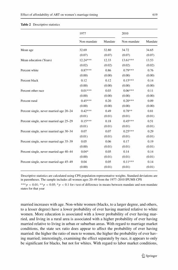
Descriptive statistics for the sample can be found in Table 2. They are presentedfor the first and last years of the sample by whether the state ever enacted a mandatein the sample period. In general, an aging, greater educational attainment, and greaterracial diversity of the population are apparent over time. There are differences inthe education, racial composition, and urban status of the mandate and non-mandatestates, and as such, these factors are controlled for in the empirical analysis. For bothgroups, there is evidence of increasing delay of marriage over the sample period, withthe effect appearing to be stronger for the mandate states.
7 Primary results
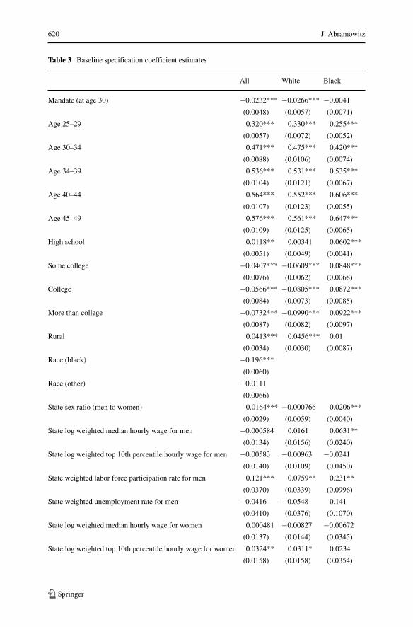
The coefficient estimates represent the difference in the probability of a woman everhaving married. The coefficient estimates for the baseline specification are presentedin Table 3.19 In general, the results show that the probability of a woman ever having
16A limitation of using CPS data as compared to Census data is that the sample sizes are smaller and thereis greater risk of serial correlation among the dependent variable as discussed in Bertrand et al. (2004). Tomitigate this risk, robust standard errors clustered by state are used in the empirical analysis.17Data on age at first marriage were collected as part of the CPS fertility supplements.18Data on age at first marriage are also available in the National Survey of Family Growth, although stateof residency information is not publicly available, as well as in the Panel Study of Income Dynamics, butthis dataset provides a much smaller sample size than either the Census or CPS. Further analysis using dataon age at first marriage from the Panel Study of Income Dynamics is examined in Abramowitz (2012).19In all regressions, robust standard errors clustered by state are in parentheses and ***p < 0.01; **p <
0.05; *p < 0.1.
Effect of affordability of ART on women’s marriage timing 619
Table 2 Descriptive statistics
1977 2010
Non-mandate Mandate Non-mandate Mandate
Mean age 32.69 32.80 34.72 34.65
(0.07) (0.07) (0.07) (0.07)
Mean education (Years) 12.24*** 12.33 13.61*** 13.53
(0.02) (0.02) (0.02) (0.02)
Percent white 0.87*** 0.86 0.79*** 0.76
(0.00) (0.00) (0.00) (0.00)
Percent black 0.12 0.12 0.15*** 0.14
(0.00) (0.00) (0.00) (0.00)
Percent other race 0.01*** 0.03 0.06*** 0.11
(0.00) (0.00) (0.00) (0.00)
Percent rural 0.45*** 0.20 0.20*** 0.09
(0.00) (0.00) (0.00) (0.00)
Percent single, never married age 20–24 0.42*** 0.49 0.78** 0.81
(0.01) (0.01) (0.01) (0.01)
Percent single, never married age 25–29 0.15*** 0.18 0.45*** 0.51
(0.01) (0.01) (0.01) (0.01)
Percent single, never married age 30–34 0.07 0.07 0.25*** 0.29
(0.01) (0.01) (0.01) (0.01)
Percent single, never married age 35–39 0.05 0.06 0.17 0.19
(0.00) (0.01) (0.01) (0.01)
Percent single, never married age 40–44 0.04* 0.05 0.14 0.14
(0.00) (0.01) (0.01) (0.01)
Percent single, never married age 45–49 0.04 0.05 0.11*** 0.14
(0.00) (0.01) (0.01) (0.01)
Descriptive statistics are calculated using CPS population-representative weights. Standard deviations arein parentheses. The sample includes all women ages 20–49 from the 1977–2010 IPUMS CPS
***p < 0.01; **p < 0.05; *p < 0.1 for t test of difference in means between mandate and non-mandatestates for that year
married increases with age. Non-white women (blacks, to a larger degree, and others,to a lesser degree) have a lower probability of ever having married relative to whitewomen. More education is associated with a lower probability of ever having mar-ried, and living in a rural area is associated with a higher probability of ever havingmarried relative to living in urban or suburban areas. With regard to marriage marketconditions, the state sex ratio does appear to affect the probability of ever havingmarried: the higher the ratio of men to women, the higher the probability of ever hav-ing married; interestingly, examining the effect separately by race, it appears to onlybe significant for blacks, but not for whites. With regard to labor market conditions,
State sex ratio (men to women) 0.0164*** −0.000766 0.0206***
(0.0029) (0.0059) (0.0040)
State log weighted median hourly wage for men −0.000584 0.0161 0.0631**
(0.0134) (0.0156) (0.0240)
State log weighted top 10th percentile hourly wage for men −0.00583 −0.00963 −0.0241
(0.0140) (0.0109) (0.0450)
State weighted labor force participation rate for men 0.121*** 0.0759** 0.231**
(0.0370) (0.0339) (0.0996)
State weighted unemployment rate for men −0.0416 −0.0548 0.141
(0.0410) (0.0376) (0.1070)
State log weighted median hourly wage for women 0.000481 −0.00827 −0.00672
(0.0137) (0.0144) (0.0345)
State log weighted top 10th percentile hourly wage for women 0.0324** 0.0311* 0.0234
(0.0158) (0.0158) (0.0354)
Effect of affordability of ART on women’s marriage timing 621
Table 3 (continued)
All White Black
State weighted labor force participation rate for women −0.0680* −0.0687* −0.0141
(0.0358) (0.0387) (0.1130)
State weighted unemployment rate for women 0.0594 0.0543 −0.00191
(0.0499) (0.0433) (0.1560)
Constant 0.188 0.214 −0.378
(0.1610) (0.1750) (0.4570)
Observations 1,287,116 1,069,412 142,805
R-squared 0.27 0.26 0.23
Shown are coefficients estimated from the baseline specification of the determinants of the probabilityof having ever married for the full sample and separately for whites and blacks. Each column presentsresults from a single regression. Regressions are weighted, with robust standard errors clustered at the statelevel in parentheses. Specifications include state, year, and age group fixed effects as well as individualdemographic and state-by-year level marriage market and labor market controls. The sample includes allwomen ages 20–49 from the 1977–2010 IPUMS CPS
***p < 0.01; **p < 0.05; *p < 0.1
many of the controls do not appear to affect the probability of ever having married,but this is not surprising given state-wide variation in these factors. In general, betterlabor market conditions for men appear to be associated with a higher probability ofever having married, while the effects of labor market conditions for women appearto be mixed: an increase in the top 10th percentile of their hourly wage is associatedwith a higher likelihood of marriage while an increase in the female labor forceparticipation rate appears to be associated with a lower likelihood of marriage.
As seen in Table 3, in the baseline across-ages specification, significant negativeeffects of the mandates on the probability of ever having married are found for thefull sample and for whites. The results imply that the mandates are associated with adecrease in a woman’s probability of ever having married of between two and threepercentage points. These results could indicate that women are less likely to marryat all ages: that women delay marriage at younger ages, but then do not marry atolder ages. From this specification, it is not possible to determine whether this isthe pattern of marriage timing associated with the mandates. Therefore, the analysisestimates the full specification next to identify if there are differential effects of themandates by age group. No significant effect of the mandates was found for blacks inthe baseline specification; since the effects of the mandates generally do not appearto be significant for blacks, results of further specifications will only be presented forwhites.20
While the baseline results suggest that the mandates are associated with a lowerprobability of ever having married, to ascertain whether this effect is consistent for
20The full specification was estimated separately for blacks and none of the mandate effects were found tobe significant, this is consistent with the literature analyzing the effects of the mandates on use of fertilitytreatment and likelihood of a first birth (Bitler and Schmidt 2006, 2012; Ohinata 2011).
622 J. Abramowitz
women of different ages, the full specification estimates the effects of the mandatesseparately for each age group. In this case, to find the effects of interest, the coef-ficient estimates themselves are not sufficient. The mandate–age group interactionscoefficient estimates on their own do not reflect the true effects of the mandates oneach age group as they only reflect the differential effect of the mandates on a par-ticular age group in comparison to the omitted age group. To find the effects of themandates on marriage rates, considered as the difference in the probability of everhaving married between two age groups, the coefficients on adjacent mandate–ageinteraction terms are differenced. These effects—the effects of the mandates on theprobability of marrying between each age group—are presented in Table 4.
The mandate marriage rate effects for the full specification, which includes agegroup–state and age group–year interaction controls, show an interesting pattern forthe full and white samples: it appears that the mandates are associated with womenhaving a significantly lower probability of marrying between the 20–24, 25–29, and30–34 age ranges, but then having a significantly higher probability of marrying overthe 30–34 and 35–39 age ranges. This is consistent with a pattern of marriage delay.These results suggest that the likelihood of marrying associated with the mandatesis six % lower (−0.019/0.330) over the 20–24 to 25–29 age groups, 11 % lower(−0.017/0.146) over the 25–29 to 30–34 age groups, and 22 % higher (0.011/0.052)
Table 4 Mandate marriage rate effects for whites
Full Full specification
specification excluding age
group-state and
age group-year
controls
Age 20–24 to 25–29: Age 25–29 × Mandate −0.0191* 0.0127
(0.0104) (0.0103)
Age 25–29 to 30–34: Age 30–34 × Mandate - Age 25–29 × Mandate −0.0167** 0.0358***
(0.0067) (0.0091)
Age 30–34 to 35–39: Age 35–39 × Mandate - Age 30–34 × Mandate 0.0114** 0.0277***
(0.0044) (0.0061)
Age 35–39 to 40–44: Age 40–44 × Mandate - Age 35–39 × Mandate 0.0034 0.0125***
(0.0067) (0.0039)
Age 40–44 to 45–49: Age 45–49 × Mandate - Age 40–44 × Mandate −0.0073* −0.0049
(0.0037) (0.0033)
Shown are estimated effects of the mandates on the probability of marrying between age groups full spec-ification with and without age group–year and age group–state controls for whites. Each column presentsresults from a single regression. Regressions are weighted, with robust standard errors clustered at the statelevel in parentheses. Specifications include state, year, and age group fixed effects (both specifications);age group–year and age group–state fixed effects (for the full specification only); as well as individualdemographic and state-by-year level marriage market and labor market controls (both specifications). Thesample includes all white women ages 20–49 from the 1977–2010 IPUMS CPS
***p < 0.01; **p < 0.05; *p < 0.1
Effect of affordability of ART on women’s marriage timing 623
over the 30–34 to 35–39 age groups. Interestingly, the mandates are also associatedwith women having a marginally significantly lower probability of marrying overbetween the 40–44 and 45–49 age ranges. Results estimated when excluding theage group–state and age group–year fixed effects suggest that the mandates have theeffect of increasing marriage rates between most age groups, while the full specifica-tion results suggest a pattern of marriage delay, with younger age groups less likelyto marry and older age groups more likely to marry. Since the full specification con-trols for state and year effects by age group, the results with the age group-interactedfixed effects may be attributing changes in age group marriage rates by state and overtime to the mandates. Therefore, the full specification is the preferred specificationof this analysis, and it will be used for subsequent analyses.
Given that the theoretical framework predicts and other analyses (Bitler andSchmidt 2006, 2012) have found differential effects of the mandates by educationlevel, the full specification estimated with education group interactions is presentednext. Then to determine whether the mandates are affecting men’s marriage timing,the full specification is estimated for men. Next, to put the marriage rate effects incontext, the marriage level effects for each of the full, education level, and men’sspecifications are then presented.
8 Further results
8.1 Results by education level
In order to examine whether the mandates affected various education groups differ-ently, the full specification was estimated for white women with interactions of themandate, age group, and mandate–age group terms separately for women with somecollege education or less and those with college degrees or more education. Themandate marriage rate effects results are presented in Table 5.
The mandate marriage rate effects estimated with separate controls by educationlevel yield interesting results. The results for both groups exhibit patterns of marriagedelay associated with the mandates with women being less likely to marry over the20–24, 25–29, and 30–34 age ranges and more likely to marry over the 30–34, 35–39, and 40–44 age ranges. However, the effects appear to be greater in magnitude forwomen with greater educational attainment. For white women with at least a collegedegree, the likelihood of marrying over the 20–24 to 25–29 age groups is 13 % lower(-0.043/0.333) and the likelihood of marrying over the 30–34 to 35–39 age groupsis 23 % higher (0.016/0.071) for women living in states with mandates as comparedto those living in states that do not have mandates. This is consistent with the the-oretical framework that predicts a greater incentive for delay for women with moreeducation.
8.2 Results for men
Since any changes affecting women’s marriage decisions have the potential to affectmen’s marriage decisions as well, the full specification was also estimated for white
624 J. Abramowitz
Table 5 Full specification for whites by education level mandate marriage rate effects
Some college or less
Age 20–24 to 25–29: Age 25–29 × Mandate −0.0128
(0.0082)
Age 25–29 to 30–34: Age 30–34 × Mandate - Age 25–29 × Mandate −0.022***
(0.0067)
Age 30–34 to 35–39: Age 35–39 × Mandate - Age 30–34 × Mandate 0.0084*
(0.0042)
Age 35–39 to 40–44: Age 40–44 × Mandate - Age 35–39 × Mandate 0.0041
(0.0067)
Age 40–44 to 45–49: Age 45–49 × Mandate - Age 40–44 × Mandate −0.0044
(0.0045)
College graduate or more
Age 20–24 to 25–29: Age 25–29 × Mandate −0.0432**
(0.0171)
Age 25–29 to 30–34: Age 30–34 × Mandate - Age 25–29 × Mandate −0.006
(0.0124)
Age 30–34 to 35–39: Age 35–39 × Mandate - Age 30–34 × Mandate 0.0161*
(0.0081)
Age 35–39 to 40–44: Age 40–44 × Mandate - Age 35–39 × Mandate 0.0069
(0.0069)
Age 40–44 to 45–49: Age 45–49 × Mandate - Age 40–44 × Mandate −0.0189**
(0.0078)
Shown are estimated effects of the mandates on the probability of marrying between age groups for thefull specification for whites with interactions of the mandate, age group, and mandate–age group termsestimated separately for women with some college education or less and those with college degrees ormore education. Each column presents results from a single regression. Regressions are weighted, withrobust standard errors clustered at the state level in parentheses. The specification includes state, year, agegroup, age group–year, and age group–state fixed effects as well as individual demographic and state-by-year level marriage market and labor market controls. The sample includes all white women ages 20–49from the 1977–2010 IPUMS CPS
***p < 0.01; **p < 0.05; *p < 0.1
men aged 20–59.21 Here, the coefficient estimates represent the difference in theprobability of a man being single and never married. As in the analysis for women,a man is considered to be living in a mandate state if there was a mandate enacted inthe state by the time he was 30 years old or younger. Table 6 presents the marriagerate effects results for men.
The effects of the mandates on white men follow a similar pattern to those forwomen, but with a lag. It appears that for men, the mandates are associated withlower probabilities of marrying over the 20–24, 25–29, 30–34, and 40–44 age ranges,significantly so between the 25–29 and 30–34 age ranges, but a significantly higher
21An older age interval was used for men given their older average age at first marriage.
Effect of affordability of ART on women’s marriage timing 625
Table 6 Full specification mandate effects for white men
Age 20–24 to 25–29: Age 25–29 × Mandate −0.014
(0.0125)
Age 25–29 to 30–34: Age 30–34 × Mandate - Age 25–29 × Mandate −0.0205*
(0.0113)
Age 30–34 to 35–39: Age 35–39 × Mandate - Age 30–34 × Mandate −0.0016
(0.0107)
Age 35–39 to 40–44: Age 40–44 × Mandate - Age 35–39 × Mandate −0.0031
(0.0067)
Age 40–44 to 45–49: Age 45–49 × Mandate - Age 40–44 × Mandate 0.0216**
(0.0091)
Age 45–49 to 50–54: Age 50–54 × Mandate - Age 45–49 × Mandate 0.0086
(0.0091)
Age 50–54 to 55–59: Age 55–59 × Mandate - Age 50–54 × Mandate 0.0094
(0.0070)
Shown are estimated effects of the mandates on the probability of marrying between age groups for thefull specification for white men. Each column presents results from a single regression. Regressions areweighted, with robust standard errors clustered at the state level in parentheses. The specification includesstate, year, age group, age group–year, and age group–state fixed effects as well as individual demographicand state-by-year level marriage market and labor market controls. The sample includes all white menages 20-59 from the 1977-2010 IPUMS CPS
***p < 0.01; **p < 0.05; *p < 0.1
probability of marrying between the 40–44 and 45–49 age ranges and higher prob-abilities of marrying over the 25–49, 50–54, and 55–59 age ranges, though they arenot significant. This is consistent with the pattern of marriage delay seen earlier forwomen, but lagged by 5–10 years. One explanation for this could be that these menwould have married the women who delayed marriage and so the result is that theytoo will delay marriage. Another explanation could be that the increased availabilityand affordability of ART makes older women more marriageable relative to youngerwomen, so men are finding it less costly to delay marriage. It could also be the casethat men are responding to greater availability of ART for their own infertility issues.However, given the nature of the mandates, it seems unlikely that men’s decisions inresponse to the mandates would be driving the marriage timing decisions.
8.3 Marriage level effects
The marriage rate effects presented above reflect the effects of the mandates on thelikelihood of women to marry across age groups. It can also be valuable to understandthe effects of the mandates on the proportion of women married at each age group, themarriage level effects. The marriage level effects for each age group are obtained bysumming the associated mandate term and age group–mandate interaction term. Themarriage level effects results for whites for the full specification and by educationlevel are presented in Table 7.
626 J. Abramowitz
Table 7 Mandate level effects
Full specification By education level
Full specification/some college or less
Age 20–24: Mandate 0.0132 0.0092
(0.0104) (0.0107)
Age 25–29: Age 25–29 × Mandate + Mandate −0.0059 −0.0036
(0.0067) (0.0077)
Age 30–34: Age 30–34 × Mandate + Mandate −0.0226*** −0.0256***
(0.0054) (0.0061)
Age 35–39: Age 35–39 × Mandate + Mandate −0.0112** −0.0172***
(0.0046) (0.0053)
Age 40–44: Age 40–44 × Mandate + Mandate −0.0079 −0.0131**
(0.0065) (0.0050)
Age 45–49: Age 45–49 × Mandate + Mandate −0.0152** −0.0175**
(0.0060) (0.0069)
College graduate or more
Age 20–24: Mandate 0.0396***
(0.0142)
Age 25–29: Age 25–29 × Mandate + Mandate −0.0036
(0.0096)
Age 30–34: Age 30–34 × Mandate + Mandate −0.0096
(0.0102)
Age 35–39: Age 35–39 × Mandate + Mandate 0.0065
(0.0059)
Age 40–44: Age 40–44 × Mandate + Mandate 0.0133*
(0.0078)
Age 45–49: Age 45–49 × Mandate + Mandate −0.0056
(0.0042)
Shown are estimated effects of the mandates on the probability of ever having married for each age group.Each column presents results from a single regression. Regressions are weighted, with robust standarderrors clustered at the state level in parentheses. Specifications include state, year, age group, age group–year, and age group–state fixed effects as well as individual demographic and state-by-year level marriagemarket and labor market controls. The sample includes all white women ages 20–49 from the 1977–2010IPUMS CPS
***p < 0.01; **p < 0.05; *p < 0.1
The marriage level effects of the full specification suggest that the mandates areassociated with women having significantly lower probabilities of ever having mar-ried at the 30–34, 35–39, and 45–49 age ranges. Together with the marriage rateeffects presented earlier, this indicates that while the mandates might be associatedwith women delaying marriage, it still appears that fewer women ever marry by the45–49 age group. Analyzing these results by education level reveals that these effects
Effect of affordability of ART on women’s marriage timing 627
only persist for women with some college education or less; for women with col-lege degrees or more education, the mandates appear to have minimal effects of theproportion ever married by the 45–49 age group.
9 Robustness
To consider the robustness of the analysis, alternative estimations are performed.These estimations investigate heterogeneity of the mandates, consider alternate sam-ples, and examine as the treatment group in the analysis women at different ages ofmandate implementation.
9.1 Heterogeneity of mandates
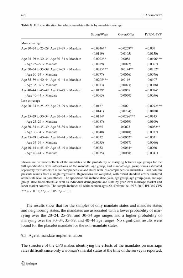
In the empirical analysis, all states with mandates related to ART were treated thesame. To understand whether different degrees of the mandates are associated withdifferent outcomes of women’s marriage rates, the full specification was estimatedwith separate controls for states with “strong” mandates, those having both mandate-to-cover laws and IVF coverage, and for states with “weak” mandates, those havingeither mandate-to-offer laws, exclusions of IVF coverage, or both. In addition, thefull specification was estimated with separate controls for states with mandate-to-cover laws and mandate-to-offer laws and with separate controls for IVF coverageand no IVF coverage. Table 8 presents these marriage rate effects results.
The results show that “strong” mandates are associated with a lower probabilityof marrying over the 20–24, 25–29, and 30–34 age ranges and a higher probabilityof marrying over the 30–34, 35–39, and 40–44 age ranges. It appears that “weak”mandates are also associated with a lower probability of marrying at younger ages,but they do not appear to be associated with a higher probability of marrying atolder ages. This is consistent with the expectation that stronger mandates should havestronger effects on women’s behavior. This pattern appears to be consistent for thecover/offer analysis. Interestingly, comparing mandate states with IVF coverage andthose without revealed little difference in marriage patterns.
9.2 Alternate samples
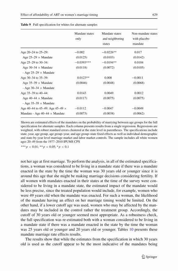
In the empirical analysis, all states were included in each specification estimated. Toexamine whether differences in the evolution of marriage attitudes between mandateand non-mandate states is what drives the results, the full specification was estimatedseparately for a sample including only states that would ever pass mandates, onlystates that would ever pass mandates and neighboring states, and only states thatdid not pass mandates with a placebo for mandate status.22 Table 9 presents thesemarriage rate effects results.
22The placebo mandate was assigned to states that did not pass mandates according to their Federal Infor-mation Processing Standard (FIPS) code with every other state being assigned a placebo mandate. Aplacebo mandate year between 1977 and 2001 was assigned to each state as a function of its FIPS code.
628 J. Abramowitz
Table 8 Full specification for whites mandate effects by mandate coverage
Strong/Weak Cover/Offer IVF/No IVF
More coverage
Age 20–24 to 25–29: Age 25–29 × Mandate −0.0246** −0.0259** −0.007
(0.0119) (0.0105) (0.0150)
Age 25–29 to 30–34: Age 30–34 × Mandate −0.0202** −0.0088 −0.0196***
- Age 25–29 × Mandate (0.0089) (0.0072) (0.0067)
Age 30–34 to 35–39: Age 35–39 × Mandate 0.0225*** 0.0144** 0.0152*
- Age 30–34 × Mandate (0.0077) (0.0056) (0.0076)
Age 35–39 to 40–44: Age 40–44 × Mandate 0.0205*** 0.0116 0.0107
- Age 35–39 × Mandate (0.0073) (0.0073) (0.0088)
Age 40–44 to 45–49: Age 45–49 × Mandate −0.0129* −0.0065 −0.0094*
- Age 40–44 × Mandate (0.0065) (0.0050) (0.0056)
Less coverage
Age 20–24 to 25–29: Age 25–29 × Mandate −0.0167 −0.009 −0.0292***
(0.0141) (0.0204) (0.0100)
Age 25–29 to 30–34: Age 30–34 × Mandate −0.0154* −0.0286*** −0.0143
- Age 25–29 × Mandate (0.0087) (0.0059) (0.0109)
Age 30–34 to 35–39: Age 35–39 × Mandate 0.0065 0.0073 0.0082**
- Age 30–34 × Mandate (0.0040) (0.0048) (0.0037)
Age 35–39 to 40–44: Age 40–44 × Mandate −0.0032 −0.0062* −0.0031
- Age 35–39 × Mandate (0.0055) (0.0037) (0.0066)
Age 40–44 to 45–49: Age 45–49 × Mandate −0.0052 −0.0064* −0.0066
- Age 40–44 × Mandate (0.0035) (0.0038) (0.0041)
Shown are estimated effects of the mandates on the probability of marrying between age groups for thefull specification with interactions of the mandate, age group, and mandate–age group terms estimatedseparately for states with more comprehensive and states with less comprehensive mandates. Each columnpresents results from a single regression. Regressions are weighted, with robust standard errors clusteredat the state level in parentheses. The specifications include state, year, age group, age group–year, and agegroup–state fixed effects as well as individual demographic and state-by-year level marriage market andlabor market controls. The sample includes all white women ages 20–49 from the 1977–2010 IPUMS CPS
***p < 0.01; **p < 0.05; *p < 0.1
The results show that for the samples of only mandate states and mandate statesand neighboring states, the mandates are associated with a lower probability of mar-rying over the 20–24, 25–29, and 30–34 age ranges and a higher probability ofmarrying over the 30–34, 35–39, and 40–44 age ranges. No significant results werefound for the placebo mandate for the non-mandate states.
9.3 Age at mandate implementation
The structure of the CPS makes identifying the effects of the mandates on marriagerates difficult since only a woman’s marital status at the time of the survey is reported,
Effect of affordability of ART on women’s marriage timing 629
Table 9 Full specification for whites for alternate samples
Mandate states Mandate states Non-mandate states
only and neighboring with placebo
states mandate
Age 20–24 to 25–29: −0.002 −0.0226** 0.017
Age 25–29 × Mandate (0.0125) (0.0103) (0.0142)
Age 25–29 to 30–34: −0.0393*** −0.0194** 0.0104
Age 30–34 × Mandate (0.0118) (0.0072) (0.0105)
- Age 25–29 × Mandate
Age 30–34 to 35–39: 0.0123** 0.008 −0.0011
Age 35–39 × Mandate (0.0046) (0.0048) (0.0068)
- Age 30–34 × Mandate
Age 35–39 to 40–44: 0.0143 0.0049 0.0012
Age 40–44 × Mandate (0.0117) (0.0075) (0.0075)
- Age 35–39 × Mandate
Age 40–44 to 45–49: Age 45–49 × −0.0112 −0.0047 −0.0049
Mandate - Age 40–44 × Mandate (0.0073) (0.0038) (0.0062)
Shown are estimated effects of the mandates on the probability of marrying between age groups for the fullspecification for alternate samples. Each column presents results from a single regression. Regressions areweighted, with robust standard errors clustered at the state level in parentheses. The specifications includestate, year, age group, age group–year, and age group–state fixed effects as well as individual demographicand state-by-year level marriage market and labor market controls. The sample includes all white womenages 20–49 from the 1977–2010 IPUMS CPS
***p < 0.01; **p < 0.05; *p < 0.1
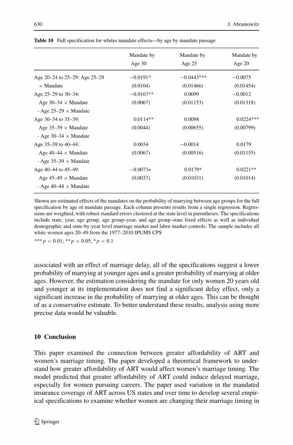
not her age at first marriage. To perform the analysis, in all of the estimated specifica-tions, a woman was considered to be living in a mandate state if there was a mandateenacted in the state by the time the woman was 30 years old or younger since it isaround this age that she might be making marriage decisions considering fertility. Ifall women with mandates enacted in their states at the time of the survey were con-sidered to be living in a mandate state, the estimated impact of the mandate wouldbe less precise, since the treated population would include, for example, women whowere 49 years old when the mandate was enacted. For such a woman, the likelihoodof the mandate having an effect on her marriage timing would be limited. On theother hand, if a lower cutoff age was used, women who may be affected by the man-dates may be included in the control rather the treatment group. Accordingly, thecutoff of 30 years old or younger seemed most appropriate. As a robustness check,the full specification was re-estimated both with a woman considered to be living ina mandate state if there was a mandate enacted in the state by the time the womanwas 25 years old or younger and 20 years old or younger. Tables 10 presents thesemandate marriage rate effects results.
The results show that while the estimates from the specification in which 30 yearsold is used as the cutoff appear to be the most indicative of the mandates being
630 J. Abramowitz
Table 10 Full specification for whites mandate effects—by age by mandate passage
Mandate by Mandate by Mandate by
Age 30 Age 25 Age 20
Age 20–24 to 25–29: Age 25–29 −0.0191* −0.0443*** −0.0075
× Mandate (0.0104) (0.01466) (0.01454)
Age 25–29 to 30–34: −0.0167** 0.0099 −0.0012
Age 30–34 × Mandate (0.0067) (0.01153) (0.01318)
- Age 25–29 × Mandate
Age 30–34 to 35–39: 0.0114** 0.0098 0.0224***
Age 35–39 × Mandate (0.0044) (0.00655) (0.00799)
- Age 30–34 × Mandate
Age 35–39 to 40–44: 0.0034 −0.0014 0.0179
Age 40–44 × Mandate (0.0067) (0.00516) (0.01155)
- Age 35–39 × Mandate
Age 40–44 to 45–49: −0.0073∗ 0.0179* 0.0221**
Age 45–49 × Mandate (0.0037) (0.01031) (0.01014)
- Age 40–44 × Mandate
Shown are estimated effects of the mandates on the probability of marrying between age groups for the fullspecification by age of mandate passage. Each column presents results from a single regression. Regres-sions are weighted, with robust standard errors clustered at the state level in parentheses. The specificationsinclude state, year, age group, age group–year, and age group–state fixed effects as well as individualdemographic and state-by-year level marriage market and labor market controls. The sample includes allwhite women ages 20–49 from the 1977–2010 IPUMS CPS
***p < 0.01; **p < 0.05, *p < 0.1
associated with an effect of marriage delay, all of the specifications suggest a lowerprobability of marrying at younger ages and a greater probability of marrying at olderages. However, the estimation considering the mandate for only women 20 years oldand younger at its implementation does not find a significant delay effect, only asignificant increase in the probability of marrying at older ages. This can be thoughtof as a conservative estimate. To better understand these results, analysis using moreprecise data would be valuable.
10 Conclusion
This paper examined the connection between greater affordability of ART andwomen’s marriage timing. The paper developed a theoretical framework to under-stand how greater affordability of ART would affect women’s marriage timing. Themodel predicted that greater affordability of ART could induce delayed marriage,especially for women pursuing careers. The paper used variation in the mandatedinsurance coverage of ART across US states and over time to develop several empir-ical specifications to examine whether women are changing their marriage timing in
Effect of affordability of ART on women’s marriage timing 631
response to greater access to ART. The results of the empirical analysis were con-sistent with the predictions of the theoretical framework. While significant negativeeffects of the mandates on the probability of ever being married were found for thefull sample and for whites for women ages 20–49, examining the marriage rates ofwomen of different age groups shows that the mandates are associated with a sig-nificantly lower probability of marrying at younger ages and a significantly higherprobability of marrying at older ages. This is consistent with the theoretical frame-work where, with greater access to ART, women who want to pursue educational andcareer opportunities delay marriage.
The results estimated with separate controls by education level show that the pat-tern of delay is apparent for women of all education levels, but appears to be strongerin magnitude for women with greater educational attainment. An interesting resultis that the mandates appear to have also had an effect on men, with men being lesslikely to marry at younger ages and then more likely to marry at older ages, similarto the pattern for women, but delayed by 5–10 years. Several explanations could beconsistent with these results; future work using more detailed data would be valuablein understanding the channels producing these results.
The marriage level effects results suggest that for the full sample of white women,while the mandates might be associated with delayed marriage, it still appears thatfewer women ever marry by the 45–49 age group, but further analysis by educationlevel reveals that this is only the case for women with some college education orless. For men, the mandates do not appear to be associated with a difference in theproportion ever married by the 45–49 age group.
Robustness checks confirm that more comprehensive mandates are associated withstronger effects on women’s marriage behavior than less comprehensive mandates.The effects of the mandates of women’s delay of marriage are robust to restricting thesample in various ways, and no significant results were found when estimating thespecification with a placebo mandate for the non-mandate states. Estimates using dif-ferent age cutoffs for inclusion in the treatment group are consistent with the patternof delay, but appear to be strongest when a cutoff of age 30 is used.
The results of the analysis are useful from a policy perspective. While the man-dates and greater availability of ART generally may have been intended to provide ameans for women and couples with fertility problems to have a child, they may havehad further reaching consequences. Greater availability of ART may have allowedwomen to delay marriage to pursue education and careers, allowing them greater life-time opportunities. However, an unintended consequence may be that women thenchoose to delay marriage and childbirth, resulting in them being more likely to facefertility problems and pursue ART procedures, which, as this paper highlighted, arevery costly relative to natural childbirths.
A drawback to the use of the mandates as an identification strategy is that while allwomen may be able to benefit by the lower cost of ART due to the mandates, somewomen may have more knowledge of the mandates and their effects on the price ofART than others. For instance, a 35-year-old woman who is concerned about her fer-tility options may have reason to obtain greater knowledge of her fertility options andtheir prices than a 25-year-old woman. On the other hand, if the diffusion of infor-mation is relatively widespread, the information gap between groups of women may
632 J. Abramowitz
be small. In addition, since the mandates can only affect the price of ART throughinsurance markets, such an identification strategy may not capture the effect of lowerprices and availability of ART on a larger scale. However, this would tend to bias theresults toward zero, so the effects of the mandates found to be significant should bevalid.
Overall, the paper makes several main contributions. First, the paper provides atheoretical framework for understanding the effect of greater affordability of ARTon women’s marriage timing. Second, the results increase our understanding of thefactors that determine women’s marriage timing. Third, the paper identifies a newconsequence of ART mandates—delayed marriage—and reveals that the mandatesaffect both younger women through their expectations about their future fertility inaddition to older women regardless of whether they will ever actually use ART.
Acknowledgments I am grateful to Shelly Lundberg, Seik Kim, Judith Thornton, Robert Plotnick,Anirban Basu, and Elaina Rose for their invaluable feedback. I would also like to thank seminar partic-ipants at the 2011 Western Economics Association International annual meetings and 2012 Society ofLabor Economists annual meetings for their helpful comments.
References
Abramowitz J (2012) Assisted reproductive technology and women’s marriage and birth timing: durationand competing risks analyses. Unpublished manuscript
Acs G, Long SH, Marquis MS, Short PF (1996) Self-insured employer health plans: prevalence, profile,provisions, and premiums. Health Aff (Project Hope) 15(2):266–278
Akerlof GA, Yellen JL, Katz ML (1996) An analysis of out-of-wedlock childbearing in the United States.Q J Econ 111(2):277–317
American Society for Reproductive Medicine (2011) State infertility insurance laws. http://asrm.org/insurance.aspx. Accessed 31 Oct 2011
Appleton SF, Pollak RA (2011) Exploring the connections between adoption and IVF: twibling analyses.Minn Law Rev Headnotes 95:60–80. Washington University in St. Louis Legal Studies ResearchPaper No. 11-05-02
Bailey M (2006) More power to the pill: the impact of contraceptive freedom on women’s life cycle laborsupply. Q J Econ 121(1):289–320
Becker GS (1973) A theory of marriage: Part I. J Polit Econ 81(4):813–846Becker GS (1974) A theory of marriage: Part II. J Polit Econ 82(2):S11–S26Becker GS (1981) A treatise on the family. Harvard University Press, CambridgeBertrand M, Duflo E, Mullainathan S (2004) How much should we trust differences-in-differences
estimates? Q J Econ 119(1):249–275Bitler MP (2008) Effects of increased access to infertility treatment on infant and child health: evidence
from health insurance mandates. NBER/IZA/University of California-Irvine, unpublished manuscriptBitler M, Schmidt L (2006) Health disparities and infertility: impacts of state-level insurance mandates.
Fertil Steril 85(4):858–865Bitler M, Schmidt L (2012) Utilization of infertility treatments: the effects of insurance mandates. Demogr
49(1):125–149Blau FD, Kahn LM, Waldfogel J (2000) Understanding young women’s marriage decisions: the role of
labor and marriage market conditions. Ind Labor Relat Rev 53(4):624–647Buckles KS (2005) Stopping the biological clock: fertility therapies and the career/family tradeoff. Boston
University, unpublished manuscriptBuckles KS (2012) Infertility insurance mandates and multiple births. Health Econ 22(7):775–789Bumpass LL, Sweet JA, Cherlin A (1991) The role of cohabitation in declining rates of marriage. J
Effect of affordability of ART on women’s marriage timing 633
Bundorf MK, Henne M, Baker L (2007) Mandated health insurance benefits and the utilization andoutcomes of infertility treatments. NBER Working Paper No. 12820
Centers for Disease Control and Prevention, American Society for Reproductive Medicine, Societyfor Assisted Reproductive Technology (2010) 2008 assisted reproductive technology success rates:national summary and fertility clinic reports. U.S. Department of Health and Human Services, Atlanta
Centers for Disease Control and Prevention, National Center for Health Statistics (2011) VitalStats. http://www.cdc.gov/nchs/vitalstats.htm. Accessed 26 Sept 2011
Cohen IG, Chen DL (2011) Trading-off reproductive technology and adoption: does subsidizing IVFdecrease adoption rates and should it matter? Minn Law Rev 95(2):485–577
Goldin C (2006) The ‘quiet revolution’ that transformed women’s employment, education, and family.Am Econ Rev 96(2):1–21
Goldin C, Katz LF (2002) The power of the pill: oral contraceptives and women’s career and marriagedecisions. J Polit Econ 110(4):730–770
Goode WJ (1964) The family. Prentice-Hall, Englewood CliffsGould ED, Paserman MD (2003) Waiting for Mr. Right: rising inequality and declining marriage rates. J
Urban Econ 53(2):257–281Hamilton BH, McManus B (2012) The effects of insurance mandates on choices and outcomes in infertility
treatment markets. Health Econ 21(8):994–1016Jain T, Harlow BL, Hornstein MD (2002) Insurance coverage and outcomes of in vitro fertilization. N
Engl J Med 347:661–666Jensen GA, Morrisey MA (1999) Employer-sponsored health insurance and mandated benefit laws.
Milbank Q 77(4):425–459King L, Meyer MH (1997) The politics of reproductive benefits: U.S. insurance coverage of contraceptive
and infertility treatments. Gend Soc 11(1):8–30King M, Ruggles S, Alexander JT, Flood S, Genadek K, Schroeder MB, Trampe B, Vick R (2010)
Integrated public use microdata series, current population survey: version 3.0 [Machine-readabledatabase]. University of Minnesota, Minneapolis
Lahey JN (2012) The efficiency of a group-specific mandated benefit revisited: the effect of infertilitymandates. J Policy Anal Manage 31(1):63–92
Loughran D (2002) The effect of male wage inequality on female age at first marriage. Rev Econ Stat84(2):237–250
Modell J (1985) Historical reflections on American marriage. In: Davis K, Grossbard-ShechtmanS (eds) Contemporary marriage: comparative perspectives on a changing institution. Russell SageFoundation, New York, pp 181–196
Myers CK (2012) Power of the pill or power of abortion? Re-examining the effects of young women’saccess to reproductive control. IZA Discussion Paper No. 6661
Ohinata A (2011) Did the US infertility health insurance mandates affect the timing of first birth? CentERWorking Paper Series No. 2011-102
RESOLVE (2011) Insurance coverage in your state. http://www.resolve.org/family-building-options/insurance coverage/state-coverage.html. Accessed 31 Oct 2011
Schmidt L (2007) Effects of infertility insurance mandates on fertility. J Health Econ 26(3):431–446Thornton A (1989) Changing attitudes toward family issues in the United States. J Marriage Fam