Turnover Liquidity and the Transmission of Monetary Policy Ricardo Lagos New York University Shengxing Zhang London School of Economics Working Paper 734 Revised January 2018 Keywords: Asset prices; Liquidity; Monetary policy; Monetary transmission JEL classification: D83, E52, G12 The views expressed herein are those of the authors and not necessarily those of the Federal Reserve Bank of Minneapolis or the Federal Reserve System. __________________________________________________________________________________________ Federal Reserve Bank of Minneapolis • 90 Hennepin Avenue • Minneapolis, MN 55480-0291 https://www.minneapolisfed.org/research/
Transcript
Turnover Liquidity and the Transmission of Monetary Policy
Ricardo Lagos New York University
Shengxing Zhang
London School of Economics
Working Paper 734
Revised January 2018
Keywords: Asset prices; Liquidity; Monetary policy; Monetary transmission JEL classification: D83, E52, G12 The views expressed herein are those of the authors and not necessarily those of the Federal Reserve Bank of Minneapolis or the Federal Reserve System. __________________________________________________________________________________________
Federal Reserve Bank of Minneapolis • 90 Hennepin Avenue • Minneapolis, MN 55480-0291
Turnover Liquidity and the Transmission of Monetary Policy
Ricardo Lagos∗
New York University
Shengxing Zhang†
London School of Economics
February 2018
Abstract
We provide empirical evidence of a novel liquidity-based transmission mechanism throughwhich monetary policy influences asset markets, develop a model of this mechanism, andassess the ability of the quantitative theory to match the evidence.
∗Lagos is thankful for the support from the C.V. Starr Center for Applied Economics at NYU, and for thehospitality of Princeton University, University College London, the University of Minnesota, and the FederalReserve Bank of Minneapolis. The views expressed herein are those of the authors and not necessarily those ofthe Federal Reserve Bank of Minneapolis or the Federal Reserve System.†Zhang is thankful for the support from the Centre for Macroeconomics at LSE and the British
Academy/Leverhulme Small Research Grant.
1 Introduction
In most modern economies, central banks implement monetary policy indirectly, by interven-
ing in certain financial markets (e.g., in the United States, the federal funds market and the
market for treasury securities). The underlying idea is that the effects of those interventions
on asset prices are transmitted to the rest of the economy to help achieve the ultimate policy
objectives. Thus, the transmission mechanism of monetary policy to asset prices is important
for understanding how monetary policy actually operates.
In this paper, we conduct an empirical, theoretical, and quantitative study of the effects
of monetary policy on financial markets in general and the equity market in particular. We
make three contributions. First, we provide empirical evidence of a novel channel through
which monetary policy influences financial markets: tight money increases the opportunity
cost of holding the nominal assets used routinely to settle financial transactions (e.g., bank
reserves, money balances), making these payment instruments scarcer. In turn, this scarcity
reduces the resalability of financial assets, and this increased illiquidity leads to a reduction in
price. We label this mechanism the turnover-liquidity (transmission) mechanism (of monetary
policy). Second, to gain a deeper understanding of this mechanism, we develop a theory of
trade in financial over-the-counter (OTC) markets (that nests the competitive benchmark as
a special case) in which money is used as a medium of exchange in financial transactions.
The model shows how the details of the market microstructure and the quantity of money
shape the performance of financial markets (e.g., as gauged by standard measures of market
liquidity), contribute to the determination of asset prices (e.g., through the resale option value
of assets), and—consistent with the evidence we document—offer a liquidity-based explanation
for the negative correlation between real stock returns and unexpected increases in the nominal
interest rate that is used to implement monetary policy. Third, we bring the theory to the
data. We calibrate a generalized version of the basic model and use it to conduct quantitative
theoretical exercises designed to assess the ability of the theory to match the empirical effects
of monetary policy on asset prices, both on policy announcement days and at longer horizons.
The rest of the paper is organized as follows. Section 2 presents the basic model. It
considers a setting in which a financial asset that yields a dividend flow of consumption goods
(e.g., an equity or a real bond) is demanded by investors who have time-varying heterogeneous
valuations for the dividend. To achieve the gains from trade that arise from their heterogeneous
2
valuations, investors participate in a bilateral market with random search that is intermediated
by specialized dealers who have access to a competitive interdealer market. In the dealer-
intermediated bilateral market, which has many of the stylized features of a typical OTC
market structure but also nests the perfectly competitive market structure as a special case,
investors and dealers seek to trade the financial asset using money as a means of payment.
Periodically, dealers and investors are also able to rebalance their portfolios in a conventional
Walrasian market. Equilibrium is characterized in Section 3. Section 4 presents the main
implications of the theory. Asset prices and conventional measures of financial liquidity (e.g.,
spreads, trade volume, and dealer supply of immediacy) are determined by the (real) quantity
of money and the details of the microstructure where the asset trades (e.g., the degree of market
power of dealers and the ease with which investors find counterparties). Generically, asset prices
in the monetary economy exhibit a speculative premium whose size varies systematically with
the market microstructure and the monetary policy stance. For example, a high anticipated
opportunity cost of holding money reduces equilibrium real balances and distorts the asset
allocation by causing too many assets to remain in the hands of investors with relatively low
valuations, which depresses real asset prices.
Section 5 is purely empirical. In it we revisit the finding, documented in previous empirical
work, that surprise increases in the nominal policy rate cause sizable reductions in real stock
returns on announcement days of the Federal Open Market Committee (FOMC). A 1 basis
point unexpected increase in the policy rate causes a decrease of between 5 and 11 basis points
in the stock market return on the day of the policy announcement. In addition, this section
contains two new empirical findings. First, we document that episodes of unexpected policy
tightening are also associated with large and persistent declines in stock turnover. Second, we
find evidence that the magnitude of the reduction in return caused by the policy tightening is
significantly larger for stocks that are normally traded more actively, e.g., stocks with higher
turnover rates. For example, in response to an unexpected increase in the policy rate, the
announcement-day decline in the return of a stock in the 95th percentile of turnover rates is
about 2.5 times larger than that of a stock in the 5th percentile. The empirical evidence in this
section suggests a mechanism whereby monetary policy affects asset prices through a reduction
in turnover liquidity.
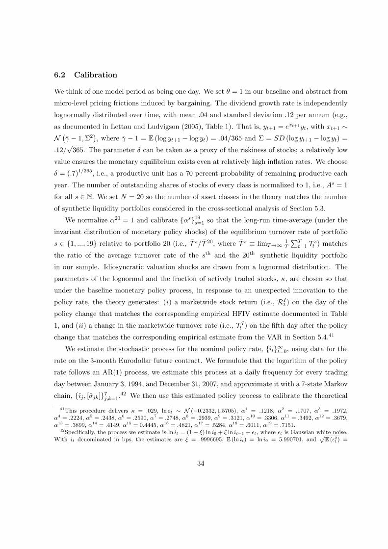
In Section 6 we formulate, calibrate, and simulate a generalized version of the basic model
and use it to assess the ability of the theory to fit the empirical evidence on the effects of
3
monetary shocks on aggregate stock returns as well as the new cross-sectional evidence on
the turnover-liquidity transmission mechanism. Section 7 concludes. Appendix A contains
all proofs. Appendices B, C, D, and E, contain supplementary material. Appendix B covers
technical aspects of the data, estimation, and simulation. Appendix C contains additional
theoretical derivations and results. Appendix D verifies the robustness of the empirical and
quantitative findings. This paper is related to four areas of research: search-theoretic models
of money, search-theoretic models of financial trade in OTC markets, resale option theories of
asset price bubbles, and an extensive empirical literature that studies the effects of monetary
policy on asset prices. Appendix E places our contribution in the context of all these literatures.
2 Model
Time is represented by a sequence of periods indexed by t = 0, 1, .... Each period is divided
into two subperiods where different activities take place. There is a continuum of infinitely
lived agents called investors, each identified with a point in the set I = [0, 1]. There is also a
continuum of infinitely lived agents called dealers, each identified with a point in the set D =
[0, 1]. All agents discount payoffs across periods with the discount factor β ≡ 1/ (1 + r), where
r > 0 denotes the real interest rate. In every period, there is a continuum of active production
units with measure As ∈ R++. Every active unit yields an exogenous dividend yt ∈ R+ of a
perishable consumption good at the end of the first subperiod of period t. (Each active unit
yields the same dividend as every other active unit, so ytAs is the aggregate dividend.) At the
beginning of every period, every active unit is subject to an independent idiosyncratic shock
that renders it permanently unproductive with probability 1 − δ ∈ [0, 1). If a production unit
remains active, its dividend in period t is yt = γtyt−1 where γt is a nonnegative random variable
with cumulative distribution function Γ, i.e., Pr (γt ≤ γ) = Γ (γ), and mean γ ∈ (0, (βδ)−1).
The time t dividend becomes known to all agents at the beginning of period t, and at that
time each failed production unit is replaced by a new unit that yields dividend yt in the initial
period and follows the same stochastic process as other active units thereafter (the dividend of
the initial set of production units, y0 ∈ R++, is given at t = 0). In the second subperiod of
every period, every agent has access to a linear production technology that transforms effort
into a perishable homogeneous consumption good.
For each active production unit, there is a durable and perfectly divisible equity share
that represents the bearer’s ownership of the production unit and confers him the right to
4
collect dividends. At the beginning of every period t ≥ 1, each investor receives an endowment
of (1− δ)As equity shares corresponding to the new production units. (When a production
unit fails, its equity share disappears.) There is a second financial instrument, money, that
is intrinsically useless (it is not an argument of any utility or production function, and unlike
equity, ownership of money does not constitute a right to collect any resources). The stock
of money at time t is denoted Amt . The initial stock of money, Am0 ∈ R++, is given and
Amt+1 = µAmt , with µ ∈ R++. A monetary authority injects or withdraws money via lump-sum
transfers or taxes to investors in the second subperiod of every period. At the beginning of
period t = 0, each investor is endowed with a portfolio of equity shares and money. All financial
instruments are perfectly recognizable, cannot be forged, and can be traded in every subperiod.
In the second subperiod of every period, all agents can trade the consumption good produced
in that subperiod, equity shares, and money in a spot Walrasian market. In the first subperiod
of every period, trading is organized as follows. Investors can trade equity shares and money
in a random bilateral OTC market with dealers, while dealers can also trade equity shares and
money with other dealers in a spot Walrasian interdealer market. We use α ∈ [0, 1] to denote
the probability that an individual investor is able to make contact with a dealer in the OTC
market. (The probability that a dealer contacts an investor is also α.) Once a dealer and an
investor have contacted each other, the pair negotiates the quantity of equity shares and money
that the dealer will trade in the interdealer market on behalf of the investor and a fee for the
dealer’s intermediation services. We assume the terms of the trade between an investor and a
dealer in the OTC market are determined by Nash bargaining where θ ∈ [0, 1] is the investor’s
bargaining power. The timing is that the round of OTC trade takes place in the first subperiod
and ends before production units yield dividends. Hence equity is traded cum dividend in
the OTC market (and in the interdealer market) of the first subperiod and ex dividend in the
Walrasian market of the second subperiod.1 Asset purchases in the OTC market cannot be
financed by borrowing (e.g., due to anonymity and lack of commitment and enforcement). This
assumption and the structure of preferences described below create the need for a medium of
exchange in the OTC market.
1As in previous search models of OTC markets, e.g., see Duffie et al. (2005) and Lagos and Rocheteau (2009),an investor must own the equity share in order to consume the dividend.
5
An individual dealer’s preferences are represented by
Ed0∞∑t=0
βt(cdt − hdt),
where cdt is his consumption of the homogeneous good that is produced, traded, and consumed
in the second subperiod of period t, and hdt is the utility cost from exerting hdt units of effort
to produce this good. The expectation operator Ed0 is with respect to the probability measure
induced by the dividend process and the random trading process in the OTC market. Dealers
get no utility from the dividend good.2 An individual investor’s preferences are represented by
E0
∞∑t=0
βt (εityit + cit − hit) ,
where yit is the quantity of the dividend good that investor i consumes at the end of the first
subperiod of period t, cit is his consumption of the homogeneous good that is produced, traded,
and consumed in the second subperiod of period t, and hit is the utility cost from exerting hit
units of effort to produce this good. The variable εit denotes the realization of a valuation shock
that is distributed independently over time and across agents, with a differentiable cumulative
distribution function G on the support [εL, εH ] ⊆ [0,∞], and ε =∫εdG (ε). Investor i learns
his realization εit at the beginning of period t, before the OTC trading round. The expectation
operator E0 is with respect to the probability measure induced by the dividend process, the
investor’s valuation shock, and the random trading process in the OTC market.
Consider a social planner who wishes to maximize the sum of all agents’ expected discounted
utilities subject to the same meeting frictions that agents face in the decentralized formulation.
Specifically, in the first subperiod of every period, the planner can only reallocate assets among
all dealers and the measure α of investors who contact dealers at random. In Appendix C
(Proposition 9 in Section C.1), we prove the allocation that solves the planner’s problem is
characterized by the following two properties: (a) only dealers carry equity between periods,
and (b) among those investors who have a trading opportunity with a dealer in the OTC market,
only those with the highest valuation hold equity shares at the end of the first subperiod.
2This assumption implies that dealers have no direct consumption motive for holding the equity share. It iseasy to relax, but we adopt it because it is the standard benchmark in the search-based OTC literature, e.g., seeDuffie et al. (2005), Lagos and Rocheteau (2009), Lagos, Rocheteau, and Weill (2011), and Weill (2007).
6
3 Equilibrium
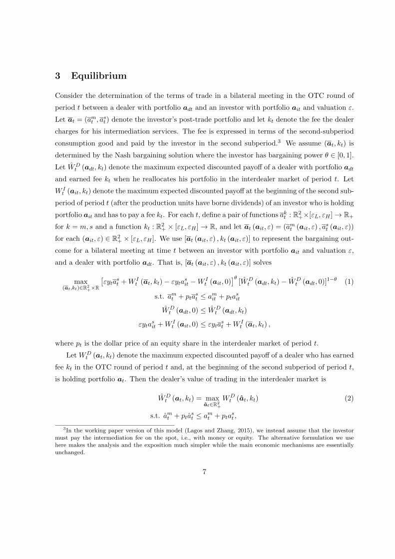
Consider the determination of the terms of trade in a bilateral meeting in the OTC round of
period t between a dealer with portfolio adt and an investor with portfolio ait and valuation ε.
Let at = (amt , ast ) denote the investor’s post-trade portfolio and let kt denote the fee the dealer
charges for his intermediation services. The fee is expressed in terms of the second-subperiod
consumption good and paid by the investor in the second subperiod.3 We assume (at, kt) is
determined by the Nash bargaining solution where the investor has bargaining power θ ∈ [0, 1].
Let WDt (adt, kt) denote the maximum expected discounted payoff of a dealer with portfolio adt
and earned fee kt when he reallocates his portfolio in the interdealer market of period t. Let
W It (ait, kt) denote the maximum expected discounted payoff at the beginning of the second sub-
period of period t (after the production units have borne dividends) of an investor who is holding
portfolio ait and has to pay a fee kt. For each t, define a pair of functions akt : R2+×[εL, εH ]→ R+
for k = m, s and a function kt : R2+ × [εL, εH ]→ R, and let at (ait, ε) = (amt (ait, ε) , a
st (ait, ε))
for each (ait, ε) ∈ R2+ × [εL, εH ]. We use [at (ait, ε) , kt (ait, ε)] to represent the bargaining out-
come for a bilateral meeting at time t between an investor with portfolio ait and valuation ε,
and a dealer with portfolio adt. That is, [at (ait, ε) , kt (ait, ε)] solves
max(at,kt)∈R2
+×R
[εyta
st +W I
t (at, kt)− εytasit −W It (ait, 0)
]θ[WD
t (adt, kt)− WDt (adt, 0)]1−θ (1)
s.t. amt + ptast ≤ amit + pta
sit
WDt (adt, 0) ≤ WD
t (adt, kt)
εytasit +W I
t (ait, 0) ≤ εytast +W It (at, kt) ,
where pt is the dollar price of an equity share in the interdealer market of period t.
Let WDt (at, kt) denote the maximum expected discounted payoff of a dealer who has earned
fee kt in the OTC round of period t and, at the beginning of the second subperiod of period t,
is holding portfolio at. Then the dealer’s value of trading in the interdealer market is
WDt (at, kt) = max
at∈R2+
WDt (at, kt) (2)
s.t. amt + ptast ≤ amt + pta
st ,
3In the working paper version of this model (Lagos and Zhang, 2015), we instead assume that the investormust pay the intermediation fee on the spot, i.e., with money or equity. The alternative formulation we usehere makes the analysis and the exposition much simpler while the main economic mechanisms are essentiallyunchanged.
7
where at ≡ (amt , ast ). For each t, define a pair of functions, akt : R2
+ → R+ for k = m, s, and let
at (at) = (amt (at) , ast (at)) denote the solution to (2).
Let V Dt (at) denote the maximum expected discounted payoff of a dealer who enters the
OTC round of period t with portfolio at ≡ (amt , ast ). Let φt ≡ (φmt , φ
st ), where φmt is the real
price of money and φst the real ex dividend price of equity in the second subperiod of period t
(both expressed in terms of the second subperiod consumption good). Then,
WDt (at, kt) = max
(ct,ht,at+1)∈R4+
[ct − ht + βEtV D
t+1 (at+1)]
(3)
s.t. ct + φtat+1 ≤ ht + kt + φtat,
where at+1 ≡(amt+1, a
st+1
), at+1 =
(amt+1, δa
st+1
), Et is the conditional expectation over the next-
period realization of the dividend, and φtat denotes the dot product of φt and at. Similarly,
let V It (at, ε) denote the maximum expected discounted payoff of an investor with valuation ε
and portfolio at ≡ (amt , ast ) at the beginning of the OTC round of period t. Then,
W It (at, kt) = max
(ct,ht,at+1)∈R4+
[ct − ht + βEt
∫V It+1
(at+1, ε
′) dG(ε′)
](4)
s.t. ct + φtat+1 ≤ ht − kt + φtat + Tt,
where at+1 = (amt+1, δast+1 + (1− δ)As) and Tt ∈ R is the real value of the time t lump-sum
monetary transfer.
The value function of an investor who enters the OTC round of period t with portfolio at
and valuation ε is
V It (at, ε) = α
εyta
st (at, ε) +W I
t [at (at, ε) , kt (at, ε)]
+ (1− α)[εyta
st +W I
t (at, 0)].
The value function of a dealer who enters the OTC round of period t with portfolio at is
V Dt (at) = α
∫WDt [at, kt (ait, ε)] dHIt (ait, ε) + (1− α) WD
t (at, 0) ,
where HIt is the joint cumulative distribution function over the portfolios and valuations of the
investors the dealer may contact in the OTC market of period t.
Let j ∈ D, I denote the agent type, i.e., “D” for dealers and “I” for investors. Then for
j ∈ D, I, let Amjt and Asjt denote the quantities of money and equity shares, respectively, held
by all agents of type j at the beginning of the OTC round of period t (after production units have
depreciated and been replaced). That is, Amjt =∫amt dFjt (at) and Asjt =
∫astdFjt (at), where
8
Fjt is the cumulative distribution function over portfolios at = (amt , ast ) held by agents of type j
at the beginning of the OTC round of period t. Let Amjt+1 and Asjt+1 denote the total quantities
of money and shares held by all agents of type j at the end of period t, i.e., AkDt+1 =∫D a
kjt+1dj
and AkIt+1 =∫I a
kit+1di for k ∈ s,m, with AmDt+1 = AmDt+1, AsDt+1 = δAsDt+1, AmIt+1 = AmIt+1,
and AsIt+1 = δAsIt+1 + (1− δ)As. Let AmDt and AsDt denote the quantities of money and shares
held after the OTC round of trade of period t by all the dealers, and let AmIt and AsIt denote the
quantities of money and shares held after the OTC round of trade of period t by all the investors
who are able to trade in the first subperiod. For asset k ∈ s,m, AkDt =∫akt (at) dFDt (at)
and AkIt = α∫akt (at, ε)dHIt(at, ε). We are now ready to define an equilibrium.
Definition 1 An equilibrium is a sequence of prices, 1/pt, φmt , φst∞t=0, bilateral terms of trade
in the OTC market, at, kt∞t=0, dealer portfolios, 〈adt, adt+1,adt+1〉d∈D∞t=0, and investor port-
folios, 〈ait+1,ait+1〉i∈I∞t=0, such that for all t: (i) the bilateral terms of trade at, kt∞t=0 solve
(1), (ii) taking prices and the bargaining protocol as given, the portfolios 〈adt, adt+1,adt+1〉 solve
the individual dealer’s optimization problems (2) and (3), and the portfolios 〈ait+1,ait+1〉 solve
the individual investor’s optimization problem (4), and (iii) prices, 1/pt, φmt , φst∞t=0, are such
that all Walrasian markets clear, i.e., AsDt+1 + AsIt+1 = As (the end-of-period t Walrasian mar-
ket for equity clears), AmDt+1 + AmIt+1 = Amt+1 (the end-of-period t Walrasian market for money
clears), and AkDt + AkIt = AkDt + αAkIt for k = s,m (the period t OTC interdealer markets for
equity and money clear). An equilibrium is “monetary” if φmt > 0 for all t and “nonmonetary”
otherwise.
The following result characterizes the equilibrium post-trade portfolios of dealers and in-
vestors in the OTC market, taking beginning-of-period portfolios as given.
Lemma 1 Define ε∗t ≡ptφmt −φst
ytand
χ (ε∗t , ε)
= 1 if ε∗t < ε∈ [0, 1] if ε∗t = ε= 0 if ε < ε∗t .
Consider a bilateral meeting in the OTC round of period t between a dealer and an investor
with portfolio at and valuation ε. The investor’s post-trade portfolio, [amt (at, ε) , ast (at, ε)], is
given by
amt (at, ε) = [1− χ (ε∗t , ε)] (amt + ptast )
ast (at, ε) = χ (ε∗t , ε) (1/pt) (amt + ptast ) ,
9
and the intermediation fee charged by the dealer is
kt (at, ε) = (1− θ) (ε− ε∗t )[χ (ε∗t , ε)
1
ptamt − [1− χ (ε∗t , ε)] a
st
]yt.
A dealer who enters the OTC market with portfolio adt exits the OTC market with portfolio
Lemma 1 offers a full characterization of the post-trade portfolios of investors and dealers in
the OTC market. First, the bargaining outcome depends on whether the investor’s valuation,
ε, is above or below a cutoff, ε∗t . If ε∗t < ε, the investor uses all his cash to buy equity. If ε < ε∗t ,
he sells all his equity holding for cash. The intermediation fee earned by the dealer is equal to
a share 1− θ of the investor’s gain from trade. The dealer’s post-trade portfolio is the same as
that of an investor with ε = 0.
We focus the analysis on recursive equilibria, that is, equilibria in which aggregate equity
holdings are constant over time, i.e., AsDt = AsD and AsIt = AsI for all t, and real asset prices
are time-invariant linear functions of the aggregate dividend, i.e., φst = φsyt, ptφmt ≡ φst = φsyt,
φmt AmIt = Zyt, and φmt A
mDt = ZDyt, where Z,ZD ∈ R+ Hence, in a recursive equilibrium,
ε∗t = φs−φs ≡ ε∗, φst+1/φst = φst+1/φ
st = γt+1, φmt /φ
mt+1 = µ/γt+1, and pt+1/pt = µ. Throughout
the analysis, we let β ≡ βγ and maintain the assumption µ > β (but we consider the limiting
case µ→ β).
For the analysis that follows, it is convenient to define
µ ≡ β
[1 +
(1− αθ)(1− βδ
)(ε− ε)
ε
]and µ ≡ β
[1 +
αθ(1− βδ
)(ε− εL)
βδε+(1− βδ
)εL
], (5)
where ε ∈ [ε, εH ] is the unique solution to
ε− ε+ αθ
∫ ε
εL
(ε− ε) dG(ε) = 0. (6)
Lemma 4 (in Appendix A) establishes that µ < µ. The following proposition characterizes the
equilibrium set.
Proposition 1 (i) A nonmonetary equilibrium exists for any parametrization. (ii) There is no
recursive monetary equilibrium if µ ≥ µ. (iii) In the nonmonetary equilibrium, AsI = As−AsD =
As (only investors hold equity shares), there is no trade in the OTC market, and the equity price
in the second subperiod is
φst = φsyt, with φs =βδ
1− βδε. (7)
10
(iv) If µ ∈ (β, µ), then there is one recursive monetary equilibrium; asset holdings of dealers
and investors at the beginning of the OTC round of period t are AmDt = Amt −AmIt = 0 and
AsD = As −AsI
= δAs if β < µ < µ∈ [0, δAs] if µ = µ= 0 if µ < µ < µ
and asset prices are
φst = φsyt, with φs =
βδ
1−βδε∗ if β < µ ≤ µ
βδ1−βδ
[ε+ αθ
∫ ε∗εL
(ε∗ − ε) dG(ε)]
if µ < µ < µ(8)
φst = φsyt, with φs = ε∗ + φs (9)
φmt = ZytAmt
(10)
pt =φs
ZAmt , (11)
where
Z =αG (ε∗)AsI +AsDα [1−G (ε∗)]
(ε∗ + φs) (12)
and for any µ ∈(β, µ
), ε∗ ∈ (εL, εH) is the unique solution to(
1− βδ) ∫ εH
ε∗ (ε− ε∗) dG(ε)
ε∗ + βδ[ε− ε∗ + αθ
∫ ε∗εL
(ε∗ − ε) dG(ε)]Iµ<µ
− µ− ββαθ
= 0. (13)
(v) (a) As µ→ µ, ε∗ → εL and φst →βδ
1−βδ εyt. (b) As µ→ β, ε∗ → εH and φst →βδ
1−βδεHyt.
In the nonmonetary equilibrium, dealers are inactive and equity shares are held only by
investors. With no valued money, investors and dealers cannot exploit the gains from trade
that arise from the heterogeneity in investor valuations in the first subperiod, and the real asset
price is φs = βδ1−βδ εy, i.e., equal to the expected discounted value of the dividend stream since
the equity share is not traded. (Shares can be traded in the Walrasian market of the second
subperiod, but gains from trade at that stage are nil.) The recursive monetary equilibrium
exists only if the inflation rate is not too high, i.e., if µ < µ. In the monetary equilibrium,
the marginal valuation, ε∗, which according to Lemma 1 partitions the set of investors into
those who buy and those who sell the asset when they meet a dealer in the OTC market, is
characterized by (13) in part (iv) of Proposition 1. Unlike what happens in the nonmonetary
equilibrium, the OTC market is active in the monetary equilibrium, and it is easy to show
11
that the marginal valuation, ε∗, is strictly decreasing in the rate of inflation, i.e., ∂ε∗
∂µ < 0 (see
Corollary 3 in Appendix A). Intuitively, the real value of money falls as µ increases, so the
marginal investor valuation, ε∗, decreases, reflecting the fact that under the higher inflation rate,
the investor that was marginal under the lower inflation rate is no longer indifferent between
carrying cash and equity out of the OTC market—he prefers equity.
According to Proposition 1, 0 ≤ εL < ε∗t in the monetary equilibrium, so Lemma 1 implies
that dealers hold no equity shares at the end of the OTC round: all equity is held by investors,
in particular, by those investors who carried equity into the period but were unable to contact
a dealer, and by those investors who purchased equity shares in bilateral trades with dealers.
After the round of OTC trade, all the money supply is held by the investors who carried cash
into the period but were unable to contact a dealer, by the investors who sold equity shares
through dealers, and by those dealers who carried equity into the OTC market.
A feature of the monetary equilibrium is that dealers never hold money overnight: at the
beginning of every period t, the money supply is all in the hands of investors, i.e., AmDt = 0 and
AmIt = Amt . The reason is that access to the interdealer market allows dealers to intermediate
assets without cash. Whether it is investors or dealers who hold the equity shares overnight
depends on the inflation rate: if it is low, i.e., if µ ∈ (β, µ), then only dealers hold equity
overnight, that is, AsDt+1 = As and AsIt+1 = 0 for all t. Conversely, if the inflation rate is
high, i.e., if µ ∈ (µ, µ), then at the end of every period t, all equity shares are in the hands of
investors, i.e., AsDt+1 = 0 and AsIt+1 = As, so strictly speaking, in this case dealers only provide
brokerage services in the OTC market. The intuition for this result is as follows.4 For dealers,
the return from holding equity overnight is given by the resale price in the OTC market. If
inflation is low, ε∗t is high (the asset is priced by relatively high valuation investors), and this
means the resale price in the OTC market is high. Since dealers are sure to trade in the OTC
market every period while investors only trade with effective probability αθ, the former are
in a better position to reap the capital gains and end up holding all equity shares overnight.
Conversely, if inflation is high then ε∗t is low, so the capital gain to a dealer from carrying the
asset to sell in the OTC market is small. The benefit to investors from holding equity includes
not only the resale value in the OTC market (which is small at high inflation) but also their
own expected valuation of the dividend good, so for high inflation, the return that investors
obtain from holding equity overnight is higher than it is for dealers. For example, as µ→ µ we
4See Lagos and Zhang (2015) for a more detailed discussion.
12
have ε∗t → εL, so the dealer’s expected return from holding equity overnight is (εL+φs)γφs , while
the investor’s is (ε+φs)γφs .
Given the marginal valuation, ε∗, part (iv) of Proposition 1 gives all asset prices in closed
form. The real ex dividend price of equity (in terms of the second subperiod consumption
good), φst , is given by (8). The cum dividend dollar price of equity in the OTC market, pt, is
given by (11). The real price of money (in terms of the second subperiod consumption good),
φmt , is given by (10). The real cum dividend price of equity (in terms of the second subperiod
consumption good) in the OTC market, ptφmt = φsyt, is given by (9).
Finally, part (v)(a) states that as the rate of money creation increases toward µ, ε∗ ap-
proaches the lower bound of the distribution of valuations, εL, so no investor wishes to sell
equity in the OTC market, and as a result the allocations and prices of the monetary equilib-
rium approach those of the nonmonetary equilibrium. Part (v)(b) states that as µ decreases
toward β, ε∗ increases toward the upper bound of the distribution of valuations, εH , so only
investors with the highest valuation purchase equity in the OTC market (all other investors
wish to sell it). Moreover, since β < µ, as µ→ β only dealers hold equity overnight. Thus, we
have the following result.
Corollary 1 The allocation implemented by the recursive monetary equilibrium converges to
the efficient allocation as µ→ β.
Let qBt,k denote the nominal price in the second subperiod of period t of an N -period risk-
free pure discount nominal bond that matures in period t + k, for k = 0, 1, 2, ..., N (so k is
the number of periods until the bond matures). Imagine the bond cannot be used as means of
payment in the first subperiod.5 Then in a recursive monetary equilibrium, qBt,k = (β/µ)k, and
i = µ/β − 1 is the time t nominal yield to maturity of the bond with k periods until maturity.
Thus, the optimal monetary policy described in Corollary 1 and part (v)(b) of Proposition 1 in
which µ = β can be interpreted as a policy that implements the Friedman rule, i.e., i = 0 for
all contingencies at all dates. Since the (gross) inflation rate is φmt /φmt+1 = µ yt
yt+1≡ 1 + πt+1,
1 + i = µ/β is equivalent to
1 + i = (1 + r) (1 + π) , (14)
5Notice that even though the bond cannot be traded for equity in the OTC round of trade, it can be exchanged(or redeemed) for money at the end of the period at no cost. Hence how “illiquid” we deem this bond dependson the length of the model period. If, as in the quantitative analysis of Section 6, the model period correspondsto one trading day, then the bond is in fact very liquid, or “very close to cash” according to the usual real-worldstandards.
13
with 1 + π ≡[Et 1
1+πt+1
]−1= µ/γ.
4 Implications
In this section, we discuss the main implications of the theory. Specifically, we show how asset
prices and conventional measures of financial liquidity (spreads, trade volume, and dealer supply
of immediacy) are determined by monetary policy and the details of the microstructure where
the asset trades (e.g., the degree of market power of dealers and the ease with which investors
find counterparties). We also show that generically, asset prices in the monetary economy
exhibit a speculative premium whose size varies systematically with monetary policy and the
market microstructure.
4.1 Asset prices
In this subsection, we study the asset-pricing implications of the theory. We focus on how the
asset price depends on monetary policy and on the degree of OTC frictions as captured by the
parameters that regulate trading frequency and the relative bargaining strengths of traders.6
4.1.1 Monetary policy
The real price of equity in a monetary equilibrium is in part determined by the option available
to low-valuation investors to resell the equity to high-valuation investors. If the growth rate of
the money supply (and therefore the inflation rate) increases, equilibrium real money balances
decline and the marginal investor valuation, ε∗, decreases, reflecting the fact that under the
higher inflation rate, the investor valuation that was marginal under the lower inflation rate
is no longer indifferent between carrying cash and equity out of the OTC market—he prefers
equity. Since the marginal investor who prices equity in the OTC market has a lower valuation,
the value of the resale option is smaller, i.e., the turnover liquidity of the asset is lower, which
in turn makes the real equity price (both φs and φs) smaller. Naturally, the real value of
money, φmt , is also decreasing in the growth rate of the money supply.7 All this is formalized
in Proposition 2.
6In Appendix A (Proposition 7) we also establish the effect of a mean-preserving spread in the distributionof valuations on the equity price.
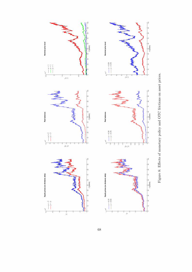
7The top row of Figure 8 (Appendix A) illustrates the typical time paths of the ex dividend equity price, φst ,real balances, φmt A
mt , and the price level, φmt , for different values of µ.
14
Proposition 2 In the recursive monetary equilibrium: (i) ∂φs/∂µ < 0, (ii) ∂φs/∂µ < 0, (iii)
∂Z/∂µ < 0 and ∂φmt /∂µ < 0.
4.1.2 OTC frictions: trading delays and market power
In the OTC market, αθ is an investor’s effective bargaining power in negotiations with dealers.
A larger αθ implies a larger gain from trade for low-valuation investors when they sell the asset
to dealers. In turn, this makes investors more willing to hold equity shares in the previous
period, since they anticipate larger gains from selling the equity in case they were to draw a
relatively low valuation in the following OTC round. Hence, real equity prices, φs and φs, are
increasing in α and θ.8 If α increases, money becomes more valuable (both Z and φmt increase),
provided we focus on a regime in which only investors carry equity overnight.9 Proposition 3
formalizes these ideas.
Proposition 3 In the recursive monetary equilibrium: (i) ∂φs/∂ (αθ) > 0, (ii) ∂φs/∂ (αθ) > 0,
(iii) ∂Z/∂α > 0 and ∂φmt /∂α > 0, for µ ∈ (µ, µ).
4.2 Financial liquidity
In this subsection, we use the theory to study the determinants of standard measures of market
liquidity: liquidity provision by dealers, trade volume, and bid-ask spreads.
4.2.1 Liquidity provision by dealers
Broker-dealers in financial markets provide liquidity (immediacy) to investors by finding them
counterparties for trade, or by trading with them out of their own account, effectively becoming
their counterparty. The following result characterizes the effect of inflation on dealers’ provision
of liquidity by accumulating assets.
Proposition 4 In the recursive monetary equilibrium: (i) dealers’ provision of liquidity by
accumulating assets, i.e., AsD, is nonincreasing in the inflation rate. (ii) For any µ close to β,
dealers’ provision of liquidity by accumulating assets is nonmonotonic in αθ, i.e., AsD = 0 for
αθ close to 0 and close to 1, but AsD > 0 for intermediate values of αθ.
8This finding is consistent with the behavior of the illiquidity premia in response to variations in the measuresof liquidity documented by Ang et al. (2013).
9Real balances can actually fall with α for µ ∈ (β, µ). The bottom row of Figure 8 (Appendix A) illustratesthe time paths of the ex dividend equity price, φst , real balances φmt A
mt , and the price level, φmt , for two different
values of α.
15
Part (i) of Proposition 4 is related to the discussion that followed Proposition 1. The expected
return from holding equity is larger for investors than for dealers with high inflation (µ > µ)
because in that case the expected resale value of equity in the OTC market is relatively low
and dealers only buy equity to resell in the OTC market, while investors also buy it with
the expectation of getting utility from the dividend flow. For low inflation (µ < µ), dealers
value equity more than investors because the OTC resale value is high and they have a higher
probability of making capital gains from reselling than investors, and this trading advantage
more than compensates for the fact that investors enjoy the additional utility from the dividend
flow. Part (ii) of Proposition 4 states that given a low enough rate of inflation, dealers’ incentive
to hold equity inventories overnight is nonmonotonic in the degree of OTC frictions as measured
by αθ. In particular, dealers will not hold inventories if αθ is either very small or very large. If
αθ is close to zero, few investors contact the interdealer market, and this makes the equity price
in the OTC market very low, which in turn implies too small a capital gain to induce dealers to
hold equity overnight. Conversely, if αθ is close to one, a dealer has no trading advantage over
an investor in the OTC market and since the investor gets utility from the dividend while the
dealer does not, the willingness to pay for the asset in the centralized market is higher for the
investor than for the dealer, and therefore it is investors and not dealers who carry the asset
overnight into the OTC market.
4.2.2 Trade volume
Trade volume is commonly used as a measure of market liquidity because it is a manifestation
of the ability of the market to reallocate assets across investors. According to Lemma 1, any
investor with ε < ε∗t who has a trading opportunity in the OTC market sells all his equity
holding. Hence, in a recursive equilibrium, the quantity of assets sold by investors to dealers
in the OTC market is Qs = αG (ε∗)AsI . From Lemma 1, the quantity of assets purchased by
investors from dealers is Qb = α [1−G (ε∗)]Amt /pt. Thus, the total quantity of equity shares
traded in the OTC market is V = Qb +Qs, or equivalently10
V = 2αG (ε∗)AsI +AsD. (15)
10To obtain (15) we used the clearing condition for the interdealer market, Qb = Qs +AsDt. Also, note that Vis trade volume in the OTC market, but since every equity share traded in the first subperiod gets retraded inthe second subperiod, total trade volume in the whole time period equals 2V.
16
Trade volume, V, depends on the growth rate of the money supply, µ, (or equivalently, inflation)
and dealers’ market power θ indirectly, through the general equilibrium effect on ε∗. A decrease
in µ or an increase in θ increases the expected return to holding money, which makes more
investors willing to sell equity for money in the OTC market, i.e., ε∗ increases and so does
trade volume, provided G′ (ε∗) > 0. In other words, the increase in turnover liquidity caused
by a decrease in µ or an increase in θ will manifest itself through an increase in trade volume
provided the cumulative distribution of investors is strictly increasing over the relevant range.
The indirect positive effect on V (through ε∗) of an increase in the investors’ trade probability
α is similar to an increase in θ, but in addition, α directly increases trade volume, since with a
higher α more investors are able to trade in the OTC market. These results are summarized in
the following proposition.
Proposition 5 In the recursive monetary equilibrium: (i) ∂V/∂µ < 0 (provided G′ (ε∗) > 0),
(ii) ∂V/∂θ > 0 (provided G′ (ε∗) > 0) and ∂V/∂α > 0.
4.2.3 Bid-ask spreads
Bid-ask spreads and intermediation fees are a popular measure of market liquidity as they
constitute the main out-of-pocket transaction cost that investors bear in OTC markets. Lemma
1 shows that when dealers execute trades on behalf of their investors, they charge a fee kt (at, ε)
that is linear in the trade size. This means that when an investor with ε > ε∗t wants to
buy equity, the dealer charges him an ask price, pat (ε) = ptφmt + (1− θ) (ε− ε∗t ) yt per share.
When an investor with ε < ε∗t wants to sell, the dealer pays him a bid price, pbt (ε) = ptφmt −
(1− θ) (ε∗t − ε) yt per share. Define Sat (ε) =pat (ε)−ptφmt
ptφmtand Sbt (ε) =
ptφmt −pbt(ε)ptφmt
, i.e., the ask
spread and bid spread, respectively, expressed as fractions of the price of the asset in the
interdealer market. Then in a recursive equilibrium, the ask spread earned by a dealer when
trading with an investor with ε > ε∗ is Sa (ε) = (1−θ)(ε−ε∗)ε∗+φs and the bid spread earned by a
dealer when trading with an investor with ε < ε∗ is Sb (ε) = (1−θ)(ε∗−ε)ε∗+φs . The average real spread
earned by dealers is S =∫ [Sa (ε) Iε∗<ε + Sb (ε) Iε<ε∗
]dG (ε). The change S in response to
changes in µ or α is ambiguous in general.11
11The reason is that the spread Sa (ε) charged to buyers is decreasing in ε∗ while the spread Sb (ε) charged tosellers may be increasing in ε∗. For example, if µ ∈
(β, µ
), it is easy to show ∂Sa (ε) /∂ε∗ = −∂Sb (ε) /∂ε∗ < 0.
17
4.3 Speculative premium
According to Proposition 1, in a monetary equilibrium the equity price, φs, is larger than
the expected present discounted value that any agent assigns to the dividend stream, i.e.,
φst ≡[βδ/(1− βδ)
]εyt. We follow Harrison and Kreps (1978) and call the equilibrium value of
the asset in excess of the expected present discounted value of the dividend, i.e., φst − φst , the
speculative premium that investors are willing to pay in anticipation of the capital gains they
will reap when reselling the asset to investors with higher valuations in the future.12 Thus, we
say investors exhibit speculative behavior if the prospect of reselling a stock makes them willing
to pay more for it than they would if they were obliged to hold it forever. Investors exhibit
speculative behavior in the sense that they buy with the expectation to resell, and naturally
the asset price incorporates the value of this option to resell.
The speculative premium in a monetary equilibrium is Pt = Pyt, where
P =
βδ
1−βδ (ε∗ − ε) if β < µ ≤ µβδ
1−βδαθ∫ ε∗εLG (ε) dε if µ < µ < µ.
The speculative premium is nonnegative in any monetary equilibrium, i.e., Pt ≥ 0, with “=”
only if µ = µ. Since ∂ε∗/∂µ < 0 (see Corollary 3), it is immediate that the speculative
premium is decreasing in the rate of inflation. Intuitively, anticipated inflation reduces the
real money balances used to finance asset trading, which limits the ability of high-valuation
traders to purchase the asset from low-valuation traders. As a result, the speculative premium is
decreasing in µ. Since ∂ε∗/∂ (αθ) > 0 (see the proof of Proposition 3), the speculative premium
is increasing in α and θ. Intuitively, the speculative premium is the value of the option to resell
the equity to a higher valuation investor in the future, and the value of this resale option to
the investor increases with the probability α that the investor gets a trading opportunity in
an OTC trading round and with the probability θ that he can capture the gains from trade in
12It is commonplace to define the fundamental value of the asset as the expected present discounted value ofthe dividend stream and to call any transaction value in excess of this benchmark a bubble. In fact, our notionof speculative premium corresponds to the notion of speculative bubble that is used in the modern literature onbubbles. See, e.g., Barlevy (2007), Brunnermeier (2008), Scheinkman and Xiong (2003a, 2003b), Scheinkman(2013), and Xiong (2013), who discuss Harrison and Kreps (1978) in the context of what is generally knownas the resale option theory of bubbles. One could argue, of course, that the relevant notion of “fundamentalvalue” should be calculated through market aggregation of diverse investor valuations and taking into accountthe monetary policy stance as well as all the details of the market structure in which the asset is traded (suchas the frequency of trading opportunities and the degree of market power of financial intermediaries), whichultimately also factor into the asset price in equilibrium. We adopt the terminology used by Harrison and Kreps(1978) to avoid semantic controversies.
18
those trades. So in low-inflation regimes, the model predicts large trade volume and a large
speculative premium. The following proposition summarizes these results.
Proposition 6 In the recursive monetary equilibrium: (i) ∂P/∂µ < 0, (ii) ∂P/∂ (αθ) > 0.
Together, Proposition 5 and Proposition 6 imply that changes in the trading probability will
generate a positive correlation between trade volume and the size of the speculative premium.
The same is true of changes in the bargaining power.13
5 Empirical analysis
According to the theory, the real asset price decreases in response to an entirely unanticipated
and permanent increase in the nominal interest rate (part (i) of Proposition 2 together with
(14)). The mechanism through which the increase in the nominal rate is transmitted to the
asset price is a reduction in turnover liquidity, i.e., a reduction in the resale option value,
accompanied by a nonpositive change in trade volume (part (i) of Proposition 5). These two
theoretical results suggest two hypotheses that can be tested with price and turnover data: (a)
surprise increases in the nominal rate reduce the marketwide stock return (and possibly trade
volume), and (b) the strength of the mechanism depends on the turnover liquidity of the stocks
(e.g., as proxied for by the turnover rate of the stock).
5.1 Data
We use daily time series for all individual common stocks in the New York Stock Exchange
(NYSE) from the Center for Research in Security Prices (CRSP).14 The daily stock return
from CRSP takes into account changes in prices and accrued dividend payment, i.e., the return
of stock s on day t is Rst =(P st +DstP st−1
− 1)× 100, where P st is the ex dividend dollar price of
stock s on day t, and Dst denotes the dollar dividend paid per share of stock s on day t. As a
measure of trade volume for each stock, we construct the daily turnover rate from CRSP, i.e.,
T st = Vst /Ast , where Vst is the trade volume of stock s on day t (measured as the total number
of shares traded) and Ast is the number of outstanding shares of stock s on day t. Whenever
13The positive correlation between trade volume and the size of the speculative premium is a feature of historicalepisodes that are usually regarded as “bubbles”—a point emphasized by Scheinkman and Xiong (2003a, 2003b)and Scheinkman (2013).
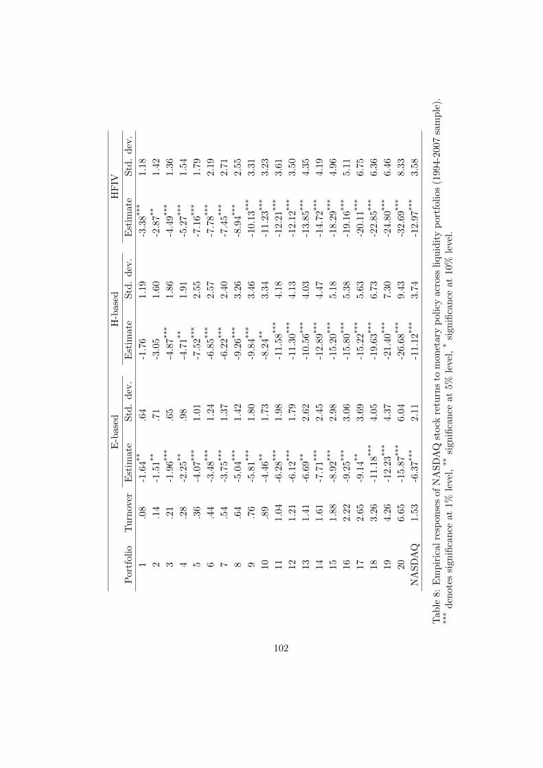
14We report results for NASDAQ stocks in Appendix D (Section D.2).
19
we use an average, e.g., of equity returns or turnover rates across a set of stocks, we use the
arithmetic average, e.g., RIt = 1n
∑ns=1Rst and T It = 1
n
∑ns=1 T st are the average return and the
average turnover rate for the universe of n common stocks listed in the NYSE.15
As a proxy for the policy (nominal interest) rate, we use the rate on the nearest Eurodollar
futures contract due to mature after the FOMC policy announcement, as in Rigobon and Sack
(2004).16 Specifically, we use the 3-month Eurodollar futures rate produced by the Chicago
Mercantile Exchange Group (CME Group) and supplied by Datastream. In some of our empir-
ical estimations, we use the tick-by-tick nominal interest rate implied by 30-day federal funds
futures and consider a high-frequency measure of the unexpected change in the nominal policy
rate in a narrow 30-minute time window around the FOMC announcement. The sample we
analyze runs from January 3, 1994 to December 31, 2007.17 The sample includes between 1300
and 1800 stocks (depending on the time period) and 133 FOMC announcement dates.18
15We report results for value-weighted returns in Appendix D (Section D.3).16Eurodollar futures are based on a $1 million face value 3-month maturity Eurodollar time deposit. These
futures contracts mature during the conventional IMM (International Monetary Market) dates in the months ofMarch, June, September, or December, extending outward 10 years into the future. In addition, at any pointin time, there are so-called 3-month Eurodollar serial contracts extending 4 months into the future that maturein months that are not conventional IMM dates. For example, at the beginning of January 2016, there arecontracts maturing in mid-March, mid-June, mid-September, and mid-December of 2016, through 2025. Thereare also serial contracts maturing in mid-January, mid-February, mid-April, and mid-May of 2016. Thus, de-pending on the timing of the FOMC announcement, the nearest contract to mature may expire between zero and30 days after the announcement. Current quotes are available at http://www.cmegroup.com/trading/interest-rates/stir/eurodollar quotes settlements futures.html. An advantage of using a futures rate as a proxy for the“policy rate” is that its movement on dates of FOMC policy announcements reflects policy surprises only anddoes not reflect anticipated policy changes. The importance of focusing on the surprise component of policyannouncements (rather than on the anticipated component) in order to identify the response of asset prices tomonetary policy was originally pointed out by Kuttner (2001) and has been emphasized by the literature sincethen, e.g., Bernanke and Kuttner (2005) and Rigobon and Sack (2004). Gurkaynak et al. (2007) offer empiricalevidence supporting the use of futures contracts as an effective proxy for policy expectations and discuss theiruse to define policy shocks.
17We start our sample period in 1994 because prior to 1994, policy changes in the federal funds target wereunannounced and frequently occurred between FOMC meetings. From 1994 onward, all changes are announcedand most coincided with FOMC meetings, so as policy announcement dates we use the dates of FOMC meetingsobtained from the website of the Board of Governors of the Federal Reserve System. The web address ishttp://www.federalreserve.gov/monetarypolicy/fomccalendars.htm. See Bernanke and Kuttner (2005) for morediscussion on the exact timing of policy announcements.
18Our full sample contains 135 policy dates. We discard two dates: 9/13/2001 and 9/17/2001 (the two atypicalFOMC announcements in the immediate aftermath of 9/11/2001). One of our estimation procedures requiresdata involving first differences in variables on the policy day and on the day preceding the policy day. In thatcase, we follow Rigobon and Sack (2004) and discard three additional policy dates because they are preceded byeither one or two holidays in financial markets. Another of our estimation procedures relies on high-frequencymarket activity in a narrow time interval around the exact time of the monetary policy announcement. In thiscase, we use the data from Gorodnichenko and Weber (2016) that consists of 118 scheduled policy dates. Foreach trading day, we discard observations whose return or turnover rate on that given day is in the top or bottom
20
In the following subsections, we use the data described above to estimate the sign and
magnitude of the effect of monetary policy on stock returns and turnover. In Subsection 5.2, we
estimate these effects for FOMC announcement days for a broad index of stocks. In Subsection
5.3, we document that the strength of the effect of monetary policy on stock returns differs
systematically with the turnover liquidity of the stock. In Subsection 5.4, we go a step further
and estimate the dynamic effects of the policy announcement on returns and turnover.
5.2 Aggregate announcement-day effects
The empirical literature has followed several approaches to estimate the impact of monetary
policy on the stock market. A popular one, known as event-study analysis, consists of estimating
the market reaction to monetary policy surprises on a subsample of trading days consisting
exclusively of the days of FOMC announcements (we denote this subsample S1). Let it denote
the day t “policy rate” (in our case, the CME Group 3-month Eurodollar future with closest
expiration date at or after day t, expressed in percentage terms) and define ∆it ≡ it − it−1.
The event-study analysis consists of running the following regression:
Y It = a+ b∆it + εt (16)
for t ∈ S1, with Y It = RIt , where εt is an exogenous shock to the asset price.19 We refer to the
estimator b as the event-study estimator (or “E-based” estimator, for short).
A concern with (16) is that it does not take into account the fact that the policy rate on
the right side may itself be reacting to asset prices (a simultaneity bias) and that a number
of other variables (e.g., news about economic outlook) are likely to have an impact on both
the policy rate and asset prices (an omitted variables bias). This concern motivates us to also
consider two other estimators: the heteroskedasticity-based estimator (“H-based” estimator,
for short) proposed by Rigobon and Sack (2004), and a version of the event-study estimator
that relies on an instrumental variable identification strategy that uses intraday high-frequency
tick-by-tick interest rate data. The H-based estimator identifies the response of asset prices
based on the heteroskedasticity of monetary policy shocks. The high-frequency instrumental
variable estimator (“HFIV” estimator, for short) addresses the omitted variable bias and the
1 percentile.19In the context of monetary policy, this approach was originally used by Cook and Hahn (1989) and has been
followed by a large number of papers, e.g., Bernanke and Kuttner (2005), Cochrane and Piazzesi (2002), Kuttner(2001), and Thorbecke (1997).
21
concern that the Eurodollar futures rate may itself respond to market conditions on policy
announcement days, by focusing on changes in a proxy for the policy rate in a very narrow
30-minute window around the time of the FOMC announcement.20
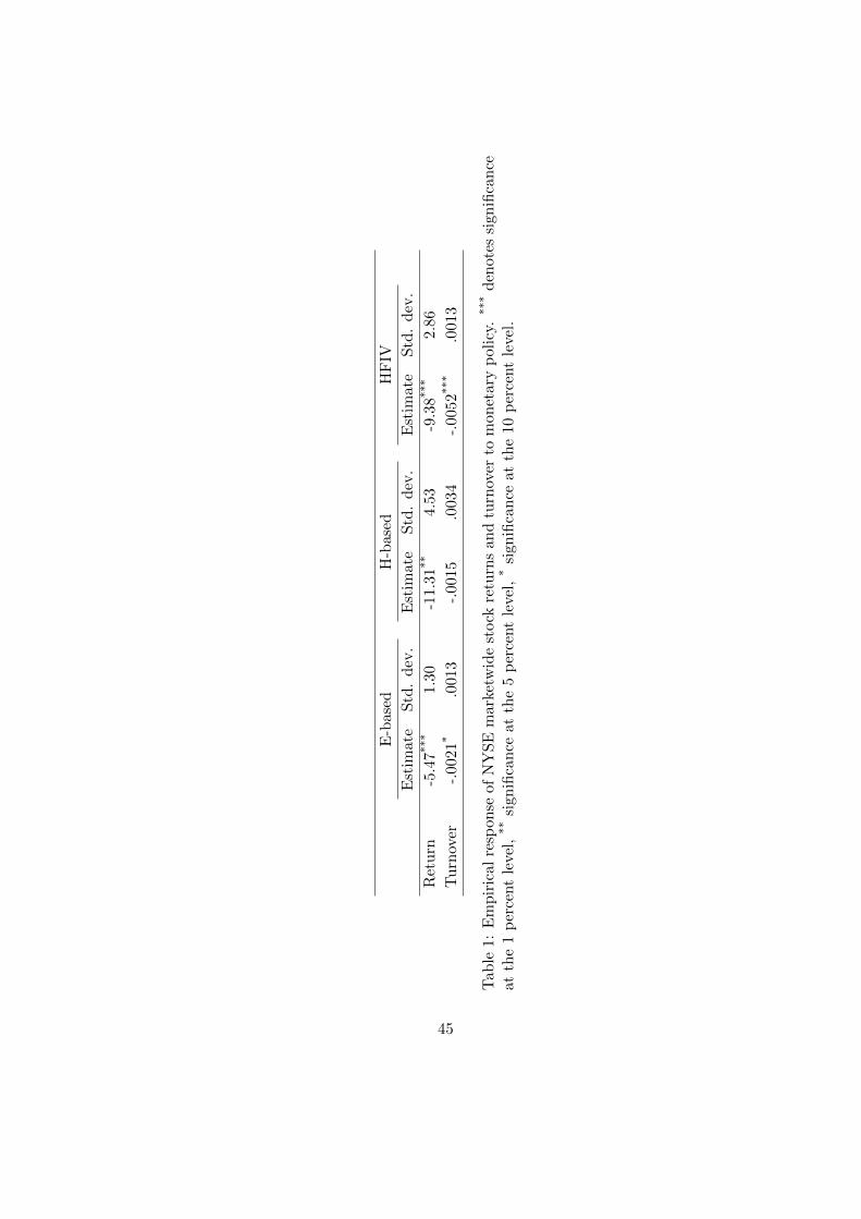
Table 1 presents the baseline results. The first column corresponds to the event-based
estimation, the second column corresponds to the heteroskedasticity-based estimation, and the
third column corresponds to the high-frequency instrumental variable estimation. Returns
are expressed in percentage terms. The first row presents estimates of the reaction of the
marketwide NYSE return to monetary policy. The point estimate for b in (16) is −5.47. This
means that a 1 basis point (bp) increase in the policy rate causes a decrease of 5.47 basis points
(bps) in the stock market return on the day of the policy announcement.21 The analogous
H-based point estimate is −11.31. These results are in line with those reported in previous
studies.22 The HFIV point estimate is −9.38, implying that a 25 bp surprise increase in the
policy rate causes a decrease in the stock market return of 2.34 percentage points (pps) on the
day of the policy announcement.23 Figure 1 shows a scatterplot with the unexpected change
in the policy rate (measure by the high-frequency change in the fed funds future rate) on the
horizontal axis, and the announcement-day marketwide stock return on the vertical axis, both
expressed in bps. The negative relationship between stock returns and fed funds rate suprises
is readily visible from the fitted line.
Previous studies have not clearly identified the specific economic mechanism that transmits
monetary policy shocks to the stock market. Conventional asset-pricing theory suggests three
broad immediate reasons why an unexpected policy nominal rate increase may lead to a decline
in stock prices. It may be associated with a decrease in expected dividend growth, with a rise
in the future real interest rates used to discount dividends, or with an increase in the expected
excess returns (i.e., equity premia) associated with holding stocks. Our theory formalizes a new
mechanism: the reduction in turnover liquidity caused by the increase in the opportunity cost
20In Appendix B we discuss the derivation of the H-based estimator (Section B.1) and describe the constructionof the HFIV estimator (Section B.2).
21The R2 indicates that 14 percent of the variance of equity prices in days of FOMC policy announcements isassociated with news about monetary policy.
22The comparable event-based estimates in Bernanke and Kuttner (2005), who focus on a different sampleperiod and measure stock returns using the value-weighted return from CRSP, range between −2.55 and −4.68.The comparable heteroskedasticity-based estimates in Rigobon and Sack (2004), who use a different series for theEurodollar forward rate, are −6.81 for the S&P 500 index, −6.5 for the WIL5000 index, −9.42 for the NASDAQ,and −4.85 for the DJIA.
23In comparing the E-based, H-based, and HFIV estimates, one should bear in mind that the number of policydates varies slightly between the three estimation methods, as explained in footnote 18.
22
of holding the nominal assets that are routinely used to settle financial transactions. To begin
assessing this mechanism, we again estimate b in (16), and the analogous H-based and HFIV
estimates, but with Y It = T It −T It−1, i.e., we use the change in the daily turnover rate averaged
over all traded stocks as the dependent variable.
The estimated effects of monetary policy announcements on the daily marketwide NYSE
turnover rate are reported in the second row of Table 1. According to the E-based estimate, a
100 bp increase in the policy rate causes a change in the level of the marketwide turnover rate
on the day of the policy announcement equal to −.0021.24 The daily marketwide turnover rate
for our sample period is .0048 (i.e., on average, stocks turn over 1.22 times during a typical
year composed of 252 trading days), which means that according to the E-based estimate, an
increase in the policy rate of 25 bps causes a reduction in the marketwide turnover rate on the
day of the policy announcement of about 10 percent of its typical level. The HFIV estimate for
a 100 bp increase in the policy rate is −.0052, implying that a 25 bp increase in the policy rate
causes a reduction in the marketwide turnover rate of about 27 percent of its typical level.
5.3 Disaggregative announcement-day effects
Another way to inspect the turnover-liquidity transmission mechanism of monetary policy is
to exploit the cross-sectional variation in turnover rates that exists across stocks. Our theory
implies that the magnitude of the change in the stock return induced by a change in the policy
rate will depend on the turnover liquidity of the stock (e.g., as measured by the turnover rate
of the stock). To test this prediction, we sort stocks into portfolios according to their turnover
liquidity, as follows. For each FOMC announcement date, t, we calculate T st as the average
turnover rate of an individual stock s over all trading days during the four weeks prior to the
day of the policy announcement. We then sort all stocks into 20 portfolios by assigning stocks
with T st ranked between the [5 (i− 1)]th percentile and (5i)th percentile to the ith portfolio,
for i = 1, ..., 20. Hence, the average turnover rate over the four-week period prior to the
announcement date for a stock in the ith portfolio is at least as large as that of a stock in the
(i− 1)th portfolio. In Table 2, the column labeled “Turnover” reports the annual turnover rate
(based on 252 trading days per year) corresponding to each of the 20 portfolios. For example,
24The R2 indicates that 3 percent of the variance of the daily turnover rate in days of FOMC policy announce-ments is associated with unexpected changes in monetary policy.
23
portfolio 1 turns over .17 times per year while portfolio 20 turns over 3.57 times per year.25
For each of the 20 portfolios, Table 2 reports the E-based, H-based, and HFIV estimates of
the annuncement-day responses of the return to a 1 percentage point (pp) increase in the policy
rate. All the estimates are negative, as predicted by the theory. Also, the magnitude of the
(statistically significant) estimates increases with the turnover liquidity of the portfolio. For
example, according to the HFIV estimates, a 1 bp increase in the policy rate causes a decrease
of 6.44 bps in the return of portfolio 1 and a decrease of 16.40 bps in the return of portfolio
20. For all three estimation methods, the relative differences in responses across portfolios are
of similar magnitude. For example, the response of the return of the most liquid portfolio is
about 2.5 times larger than the response of the least liquid portfolio.26 Figure 2 shows the
announcement-day returns of portfolio 1 (the crosses) and portfolio 20 (the circles), along with
their respective fitted lines. The larger magnitude of the response of the more liquid portfolio
is evident.
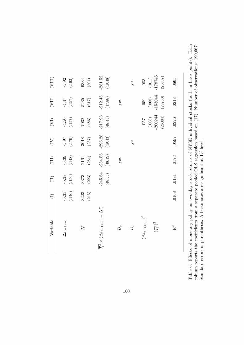
As an alternative way to estimate the heterogeneous responses of returns to monetary policy
shocks for stocks with different turnover liquidity, we ran an event-study regression of individual
stock returns (for the universe of stocks listed in the NYSE) on changes in the policy rate, an
interaction term between the change in the policy rate and individual stock daily turnover rate,
and several controls. As before, ∆it denotes the monetary policy shock on policy announcement
day t (measured by the change between day t and day t− 1 in the 3-month Eurodollar futures
contract with nearest expiration after the day t FOMC policy announcement), and T st is the
average turnover rate of the individual stock s over all the trading days during the four weeks
prior to the day of the policy announcement of day t. Let ∆i and T denote the sample averages
of ∆it and T st , respectively, and define T st ≡ (T st − T ) and ∆it ≡ (∆it −∆i). The regression
25Our motivation for constructing these liquidity-based portfolios is twofold. First, at a daily frequency,individual stock returns are extremely noisy; by grouping stocks into portfolios based on some characteristic(s)related to returns, it becomes possible to see average return differences. Second, stock-specific turnover measuresare time-varying, i.e., the turnover rate of a particular stock may change over time. Bernanke and Kuttner(2005) also examine the responses of more disaggregated indices to monetary policy shocks. Specifically, theyestimate the responses of 10 industry portfolios constructed from CRSP returns as in Fama and French (1988)but find that the precision of their estimates is not sufficient to reject the hypothesis of an equal reaction for all10 industries.
26In Appendix B (Section B.3), we report similar results from an alternative procedure that sorts stocks intoportfolios according to the strength of individual stock returns to changes in an aggregate (marketwide) measureof turnover. This alternative sorting criterion allows us to control for other differences across stocks, such as theconventional risk factors used in empirical asset-pricing models.
24
we fit is
Rst = β0 + β1∆it + β2T st + β3T st ×∆it
+Ds +Dt + β4 (∆it)2 + β5 (T st )2 + εst, (17)
where Ds is a stock fixed effect, Dt is a quarterly time dummy, and εst is the error term
corresponding to stock s on policy announcement day t. The time dummies control for omitted
variables that may affect the return of all stocks in the NYSE over time. The stock fixed
effects control for the effects that permanent stock characteristics not included explicitly in the
regression may have on individual stock returns. We include the interaction term T st × ∆it
to estimate how the effect of changes in the policy rate on individual stock returns varies
across stocks with different turnover liquidity. The coefficient of interest is β3, i.e., we want
to test whether changes in the policy rate affect individual stock returns through the stock-
specific turnover-liquidity channel. The estimate of β3 can help us evaluate whether increases
(reductions) in the policy rate cause larger reductions (increases) in returns of stocks with a
larger turnover rate, i.e., whether β3 < 0.
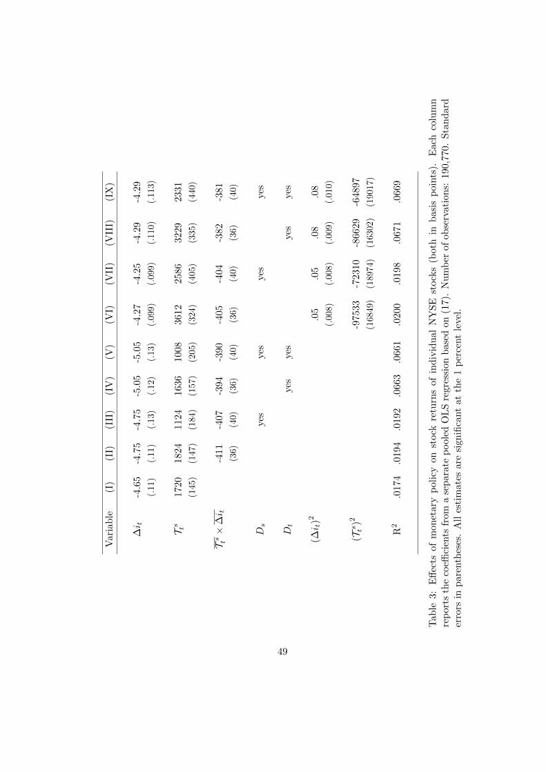
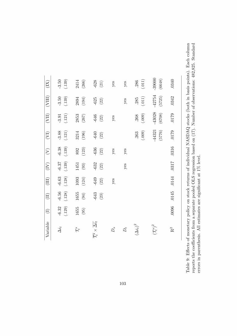
Table 3 reports the results from estimating nine different specifications based on (17). Spec-
ification (I) excludes Ds, Dt, the interaction term, T st ×∆it, and the squared terms, (∆it)2 and
(T st )2. Specification (II) adds the interaction term to specification (I). Specification (III) adds
Ds to specification (II). Specification (IV) adds Dt to specification (II). Specification (V) adds
Ds to specification (IV). Specifications (VI), (VII), (VIII), and (IX) each add the squared terms
(∆it)2 and (T st )2 to specifications (II), (III), (IV), and (V), respectively. In all specifications,
all estimates are significant at 1 percent level.27
The estimates of β1 lie near −4.5 in all specifications, implying that a 1 bp increase in the
policy rate reduces the return of a stock with average turnover by about 4.5 bps on the day of the
policy announcement.28 The estimate of interest, β3, is large and negative in all specifications.
The negative and statistically significant estimates of β3 indicate that the magnitude of the
negative effect of unexptected changes in the policy rate on announcement-day equity returns
is larger for stocks with higher turnover liquidity. To interpret the magnitude of the estimates,
consider a stock A with a daily turnover rate equal to .014 (i.e., a stock in liquidity portfolio
20) and an equity B with an annual turnover rate equal to .0007 (i.e., a stock in liquidity
27The significance of the results is not affected when we cluster standard errors by calendar date.28Recall the average daily turnover in our sample is .0048.
25
portfolio 1). Then, for example, according to specification (IX), the estimate of β3 is −381,
implying that a 1 bp increase in the policy rate reduces the announcement-day return by
β1 + 2β4 + β3
(T At − T
)≈ −8 bps for equity A and by β1 + 2β4 + β3
(T Bt − T
)≈ 3 bps for
equity B. These estimates are quite close to the E-based estimates for portfolio 20 and for
portfolio 1 reported in Table 2. Together with the findings reported in Table 1 and Table 2,
the results in Table 3 provide additional evidence that turnover liquidity is a quantitatively
important channel that transmits monetary policy shocks to asset prices.
5.4 Dynamic effects
In the previous section we documented the effect of monetary policy shocks on equity returns
and turnover on the day the policy announcement takes place. While the turnover liquidity
channel highlighted by our theory can generate the effects on announcement days documented
in the previous section, the theoretical channel is eminently dynamic. In the theory, persistent
changes in the nominal rate affect stock returns because they imply persistent changes in the
future resale value of the stock. To study the dynamic effects of monetary policy on prices and
turnover rates, we conduct a vector autoregression (VAR) analysis on the sample consisting of
all trading days between January 3, 1994 and December 31, 2007.
The baseline VAR we estimate consists of three variables, i.e.,it,RIt , T It
, where it, RIt ,
and T It are the daily measures of the policy rate, the stock return, and turnover described
in Section 5.1 and Section 5.2.29 The lag length is set to 10.30 To identify the effects of
monetary policy shocks, we apply an identification scheme based on an external high-frequency
instrument.31
29In Section 5.2, we used the change in the 3-month Eurodollar futures rate on the day of the FOMC an-nouncement as a proxy for the unexpected component of the change in the true policy rate, i.e., the effectivefederal funds rate. In this section, we instead regard the 3-month Eurodollar futures rate as the policy rate itself.We do this because, at a daily frequency, the effective federal funds rate is very volatile for much of our sample,e.g., due to institutional considerations, such as “settlement Wednesdays.” The path of the 3-month Eurodollarfutures rate is quite similar to the effective federal funds rate, but it does not display the large regulation-inducedweekly swings. In any case, we have also performed the estimation in this section using the daily effective federalfunds rate instead of the Eurodolar futures rate, and the results for returns and turnover are quite similar.
30The Akaike information criterion (AIC) suggests 10 lags, while Schwarz’s Bayesian information criterion(SBIC) and the Hannan and Quinn information criterion (HQIC) suggest 5 lags. We adopted the formulationwith 10 lags, but both formulations deliver similar estimates.
31See Appendix B (Section B.4.1) for details. The basic idea of structural vector autoregression (SVAR)identification using instruments external to the VAR can be traced back to Romer and Romer (1989) and hasbeen adopted in a number of more recent papers, including Cochrane and Piazzesi (2002), Hamilton (2003),Kilian (2008a, 2008b), Stock and Watson (2012), Mertens and Ravn (2013), and Gertler and Karadi (2015).
26
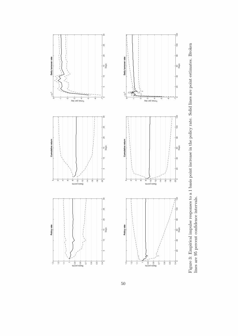
Figure 3 reports the impulse responses of the policy rate, the average cumulative stock return
between day t and day t + j defined by RIt,t+j ≡∏js=1RIt+s, and the average turnover rate,
to a 1 bp increase in the policy rate.32 The 95 percent confidence intervals forit,RIt , T It
are computed using a recursive wild bootstrap based on 10,000 replications.33 The top and
bottom rows show responses for forecast horizons of 30 days and 120 days, respectively. The
path of the policy rate is very persistent (it remains significantly above the level prevailing
prior to the shock for about 18 months). The middle panels in Figure 3 show the response
of daily cumulative stock returns. On impact, in response to the 1 bp unexpected increase
in the nominal rate, the stock return falls by about 8 bps. The magnitude of this response
on the day of the policy shock is basically the same as the HFIV point estimate reported in
Table 1. The negative effect on the stock price is quite persistent (the upper bound of the 95
percent confidence remains below zero for about 200 days). The right panels in Figure 3 show
the response of the level of the daily turnover rate. On impact, a 1 bp surprise increase in
the nominal rate causes a change in the level of the turnover rate equal to −.00005, which is
the same as the HFIV point estimate reported in Table 1. According to the estimated impulse
response, it takes about 1 day for the turnover rate to recover half of the initial drop. However,
beyond that point, the negative effect of the increase in the policy rate on turnover is quite
persistent (e.g., it takes about 110 days for it to become statistically insignificant).
In order to inspect the turnover-liquidity transmission mechanism further, we exploit the
cross-sectional variation in turnover rates across stocks and carry out the same VAR analysis
of this section but individually on each of 20 liquidity portfolios of stocks, sorted on turnover
liquidity.34 Figure 4 shows the estimated impulse responses (to a 1 bp unexpected increase in
the policy rate) of the cumulative returns of each of the twenty liquidity portfolios for a forecast
horizon of 30 days. In the figure, the darker impulse responses correspond to the portfolios with
32The impulse response for the cumulative return illustrates the path of RI−1,j−1, where j = 1, 2, ... indexesthe number of days after the policy announcement.
33The procedure is described in Appendix B (Section B.4.2). See Goncalves and Kilian (2004) for a formaleconometric analysis of this method. We compute the confindence bands for RIt,t+j by compounding theconfidence bands of the return response RIt (i.e., in the same way we compute RIt,t+j from RIt ).
34In Section 5.3 we re-sorted stocks into liquidity portfolios for each day in our sample of FOMC announcementdates (based on the average daily turnover rate over the four weeks prior to each FOMC announcement). Forthe high-frequency VAR that we estimate in this section, stocks are resorted into one of 20 liquidity portfoliosevery day. On days with no FOMC announcement, the sorting is based on daily turnover rate. On FOMCannouncement days, stocks are sorted based on their turnover rate two days prior to the announcement. Sincethe ranking of a given stock in terms of turnover tends to be quite persistent, all the sorting schemes describedhere deliver similar results.
27
higher turnover liquidity (e.g., the lightest impulse response is for portfolio 1 and the darkest,
for portfolio 20). To further illustrate the results, Figure 5 reports the impulse responses and
the corresponding 95 percent confidence intervals of the cumulative portfolio return to a 1 bp
unexpected increase in the policy rate for a forecast horizon of 30 days, for portfolios 1, 10,
and 20. Notice that the announcement-day portfolio-by-portfolio responses estimated by the
VAR line up well with the portfolio-by-portfolio HFIV estimates reported in Table 2. As in
Section 5.3, we again find that on the announcement day, the negative responses of returns
to an unexpected increase in the nominal rate tend to be larger in magnitude for portfolios
with higher turnover liquidity. However, here these responses appear to be estimated much
more precisely than in Table 2.35 Also, notice that—as will be the case in the quantitative
theory—the price responses of the portfolios with larger turnover liquidity are not only larger
in magnitude on impact, but also tend to be more persistent.36
In this section we have provided empirical evidence consistent with the turnover-liquidity
transmission mechanism of monetary policy: a persistent increase in the nominal rate reduces
the resale value of stocks, and this reduction in turnover liquidity is reflected in a persistent
price reduction and higher future stock returns.37
6 Quantitative analysis
The theoretical results we used to motivate the empirical analysis of Section 5 (e.g., part (i) of
Proposition 2 and part (i) of Proposition 5) correspond to a permanent, unanticipated increase
35Aside from the fact that the VAR specification is more flexible than (16), our VAR estimation also relies onthe HFIV identification scheme. In fact, notice that even for the simple specification (16), Table 1 and Table 2show that in general, the HFIV identification strategy by itself already delivers estimates that are more preciseand more statistically significant than the E-based and H-based estimates.
36Based on the announcement-day evidence alone, one might conjecture that the differential return responseon impact across liquidity portfolios may simply reflect that the prices of stocks with lower turnover liquiditytake longer to react to the FOMC shock. This conjecture, however, does not seem to be supported by the VARevidence in Figure 4 and Figure 5. The conjecture is also not supported by the additional regression analysis wecarry out in Appendix D (Section D.1), where we estimate the effect of an unexpected policy shock on day t onRIt−1,t+1, i.e., the cumulative stock return for the two-day horizon after the policy announcement.
37Bernanke and Kuttner (2005) is one of a few papers that has tried to identify the economic forces behind thenegative effect of nominal rate increases on stock returns. They use a VAR to decompose excess equity returnsinto components attributable to news about dividends, real interest rates, and future excess returns. Theyfind the component associated with future excess returns accounts for the largest part of the response, i.e., anincrease in the policy rate lowers stock prices mostly by increasing the expected equity premium. Bernanke andKuttner speculate this could come about via some unspecified mechanism through which tight money increasesthe riskiness of stocks (or decreases the investor’s willingness to bear risk). The turnover-liquidity mechanismwe have identified is consistent with Bernanke and Kuttner’s decomposition.
28
in the nominal rate associated with a similar increase in the growth rate of the money supply,
which while suggestive, is somewhat different from the policy shocks underlying the empirical
estimates of Section 5. Thus in order to assess the predictions and quantitative performance
of the theory, in this section we formulate, calibrate, and simulate a generalized version of the
model of Section 2.
We generalize the model along three dimensions. First, we incorporate aggregate uncertainty
in the path of monetary policy, represented by changes in the nominal interest rate implemented
via open-market operations. This extension allows us to consider theoretical experiments that
resemble more closely what goes on in financial markets, in the sense that while investors may
be surprised by the timing and size of changes in the nominal rate, they take into account
a probability distribution over future paths of the monetary policy so these changes are not
entirely unexpected. Second, we extend the model so that the innovations to the nominal policy
rate may be associated with innovations to the expected inflation rate (as in the propositions
of Section 4), as well as with innovations to the real interest rate. This extension allows us
to quantify the turnover-liquidity mechanism for settings where changes in the nominal rate
may be associated with changes in the expected inflation rate as well as with changes in the
real rate. Third, we extend the model to the case of multiple equity classes that differ in their
liquidity properties. This extension allows us to provide additional evidence for the turnover-
liquidity mechanism by exploiting the cross-sectional heterogeneity and using it to assess the
quantitative theoretical effects of monetary policy on the cross section of equity returns.
6.1 Generalized model
There are N equity classes, each indexed by s ∈ N = 1, 2, ..., N. The outstanding quantity
of equity shares of class s is As. Since the focus is on the implication of liquidity differences
across equity classes, we assume each class gives the same dividend yt, which follows the same
stochastic process described in the one-asset model of Section 2. An investor’s period t valuation
of the dividend of any equity is distributed independently over time and across investors, with
cumulative distribution function G, just as in the one-asset setup.
We model liquidity differences as follows. In each round of OTC trade, each investor can
trade equity class s ∈ N with probability αs ∈ [0, 1]. The event that the investor is able to
trade equity class s is independent of the event that he is able to trade any other equity class
n ∈ N. We interpret αs as the probability that an individual investor contacts a dealer with
29
whom he can trade equity class s. This captures the idea that dealers are specialized in trading
a particular equity class.38 In the OTC trading round there is a competitive interdealer market
for each equity class. These markets are segmented in the following sense: (i) in the OTC
trading round, equity s can only be traded in market s, and (ii) at the beginning of the period,
investors partition the money they will use for trading stocks in the first subperiod into a cash
portfolio with N components, i.e., amst s∈N, where amst is the amount of money the investor
chooses to have available to trade equity class s in the OTC market of period t. Each investor
makes this cash rebalancing decision after having observed the realization of the aggregate
state, but before learning which equity classes he will be able to trade, and before learning
his individual valuation of the dividend (the last two assumptions keep the ex post number of
investor types to a minimum). For simplicity, in this section we assume dealers do not hold
asset inventories overnight (and without loss, also that they do not hold money overnight).
In Section 2, we assumed a constant growth rate of the money supply, i.e., Amt+1 = µAmt ,
where µ ∈ R++. In this section we broaden the analysis of monetary policy along three
dimensions: (a) We allow the monetary authority to inject or withdraw money not only with
lump sum taxes, but also via open-market operations. This is a more realistic implementation
of monetary policy, and makes the theory more flexible in that it can encompass a wider range
of responses to monetary policy shocks. (b) We model monetary policy as a stochastic process.
This allows the theory to exhibit monetary policy shocks that resemble the policy surprises in
the empirical analysis of Section 5. (c) We allow monetary policy to affect market outcomes
by influencing the nominal rate through both of its components: the expected inflation rate,
and the real interest rate. This allows us to assess the robustness of the turnover-liquidity
mechanism to different degrees of passthrough from nominal rates to real rates. In summary,
we will consider general monetary policy processes that consist of three components: an open-
market operation, a change in expected inflation, and a change in the real rate. Each of these
components of the monetary policy process is modeled as follows.
38In the theory, differences in α, θ, or G all give rise to differences in turnover across assets. We focus ondifferences in α because it is conceptually the simplest and analytically the most direct way to construct assetclasses that differ in turnover liquidity. However, one could carry out the theoretical analysis by constructing assetclasses based on differences in G and θ. Differences in G work similarly to differences in α (see the equivalenceresult proved in Proposition 8, Appendix A). With regard to differences in θ, in a large class of models thatincludes this one, Duffie et al. (2005) and Lagos and Rocheteau (2009), the equilibrium asset price does notdepend on α and θ independently, but on their product, αθ. Thus, for asset-pricing purposes, differences in α canbe interpreted as capturing differences in the trading probability or in the bargaining power. The quantitativeresponse of turnover to money shocks will typically depend on whether assets differ in α or θ, however.
30
In the first subperiod, each investor can always trade in a competitive market where the
monetary authority sells Bt one-period risk-free pure-discount nominal bonds. A bond issued
in the first subperiod of t yields one dollar with certainty in the following subperiod. The
dollar price of a bond in this market is denoted qt. The bond market is segmented in the same
way as the markets for equity shares, i.e., at the beginning of period t, having observed the
realization of the monetary policy variables (but before knowing which equity classes he will be
able to trade or his dividend valuation), each investor chooses a partition of his money holdings,
amst s∈N, where N ≡ N ∪ b, and ambt denotes the amount of money the investor chooses to
have available to trade bonds in the first subperiod of t. The size of the bond issue, Bt, relative
to the size of the beginning-of-period money supply, Amt , is denoted ωt. That is, if there are
Amt dollars outstanding at the beginning of period t, in the bond market of the first subperiod
t the government sells claims to Bt = ωtAmt dollars payable in the following subperiod.
The beginning-of-period money supply evolves according to Amt+1 = [1 + (1− qt)ωt] µtAmt ,
where µt ∈ R++ denotes the growth rate of the money supply between the end of period t and
the beginning of period t+ 1 (implemented via lump-sum transfers in the second subperiod of
t). The monetary authority can implement any arbitrary process for the growth rate of the
beginning-of-period money supply, i.e., can set, Amt+1 = µtAmt for any positive path µt∞t=1,
despite the random changes in the money supply induced by the open-market operations.39
Finally, to allow for the possibility that monetary policy can affect outcomes by influencing the
real rate as well as expected inflation, we generalize the constant interest rate r of Section 2 to
a stochastic process rt∞t=1.
To summarize, we model monetary policy as a stochastic process τ t∞t=1, where τ t ≡(ωt, µt, rt). This formulation is general enough to encompass situations where monetary policy
amounts to changing expected inflation (as in monetarist models) as well as settings where
monetary policy amounts to directly influencing real rates (as in New Keynesian models). We
assume τ t∞t=1 follows a Markov chain with transition matrix σij = Pr (τ t+1 = τ j |τ t = τ i),
where τ i ≡ (ωi, µi, ri) ∈ R3++ and τ j ≡ (ωj , µj , rj) ∈ R3
++ for i, j ∈ M = 1, . . . ,M. The
realization of τ t is known at the beginning of period t.
We specialize the analysis to recursive equilibria in which prices and portfolio decisions are
time-invariant functions of an aggregate state vector that follows a time-invariant law of motion.
39Specifically, µt = µt/ [1 + (1− qt)ωt] implies Amt+1 = µtAmt for any µt∞t=1. The government budget con-
straint is Bt + Tt/φmt = Amt+1 − (Amt − qtBt), so the real lump-sum transfer (expressed in terms of the second-
subperiod consumption good) needed to implement Amt+1 = µtAmt is Tt = [(µt − 1)− (1− qt)ωt]φmt Amt .
31
The state vector is xt = (Amt , yt, τ t) ∈ R5+. Asset prices in a recursive equilibrium will be
denoted φst = φs (xt), φst = φs (xt), φ
mt = φm (xt), p
st = ps (xt), qt = q (xt), and εs∗t = εs∗ (xt).
Let Amkt denote the amount of money that investors have available to trade asset k ∈ N at the
beginning of period t (i.e., the bond, if k = b, or equity, if k ∈ N). The laws of motion for the
state variables Amt , yt, and τ t are exogenous (as described above), while Amkt = Ψk (xt) for
k ∈ N, where the decision rule Ψk is determined in equilibrium. Suppose xt = (Amt , yt, τ i) and
focus on a recursive equilibrium with the property that real prices are linear functions of the
aggregate dividend, and Ψk (xt) = λkiAmt for all k ∈ N, where λsi ∈ [0, 1] denotes the fraction of
the beginning-of-period money holdings that investors have chosen to have available to trade
asset class k in the OTC round of period t. Then, φs (xt) = φsiyt, φs (xt) ≡ ps (xt)φ
In Appendix C (Section C.3), we show that an equilibrium is characterized by a vec-
tor φsi , εs∗i , Zi, λsii∈M,s∈N of M (3N + 2) unknowns that solves the following system with
M (3N + 2) independent equations:
φsi =γδ
1 + ri
∑j∈M
σij
[ε+ φsj + αsθ
∫ εs∗j
εL
(εs∗j − ε)dG(ε)
](18)
Zi =γ
(1 + ri)µi
∑j∈M
σij
[1 + αsθ
∫ εH
εs∗j
ε− εs∗jεs∗j + φsj
dG(ε)
]Zj (19)
max(ωi/λbi , 1) = 1 + αsθ
∫ εH
εs∗i
ε− εs∗iεs∗i + φsi
dG(ε) for all (i, s) ∈M× N (20)
Ziλsi =
G (εs∗i )As
1−G (εs∗i )(εs∗i + φsi ) for all (i, s) ∈M× N (21)
1− λbi =∑s∈N
λsi for all i ∈M. (22)
In the following subsections, we calibrate and simulate this model to assess the ability of the
theory to account for the empirical findings reported in Section 5. Before doing so, it is useful
to define the theoretical analogues of the variables we studied in the empirical section.
The return of stock s at date t+ 1 is Rst+1 = φst+1/φst − 1, where φst ≡ ptφ
mt = φst + ε∗t yt is
the cum dividend price of equity at date t defined in Section 3. The real return from holding a
dollar between the end of period t and the end of period t+1 is φmt+1/φmt ≡ (1 + πt+1)−1, where
πt+1 denotes the (net) inflation rate between t and t + 1. In a recursive equilibrium, suppose
32
the state is xt = (Amt , yt, τ j) at t, and xt+1 = (µjAmt , yt+1, τ k) at t+ 1, then
1 +Rst+1 =φsk + εs∗kφsj
yt+1
yt
1 + πt+1 =ZjZk
ytyt+1
µj .
So far we have implicitly assumed that As, i.e., all outstanding equity shares of class s,
are actively traded every day. In actual markets, however, a fraction of the outstanding equity
shares are seldom traded (stocks held in 401(k) accounts, for example). Our theory remains
unchanged if we replace As with κAs for some κ ∈ [0, 1] that represents the proportion of the
universe of outstanding stocks that are actively traded, and think of the remaining (1− κ)As
as being held by nontraders outside the model. In an equilibrium in which dealers do not
hold assets (as is the case in this section), trade volume for asset class s at date t is Vst =
2αsG (εs∗t )κAs. A conventional measure of trade volume is the turnover rate used in the
empirical work of Section 5.1. According to the theory, the turnover rate on date t is
T st = Vst /As = 2αsG (εs∗t )κ.
Naturally, a nonzero fraction of inactive stocks (i.e., κ < 1) lowers the measured level of the
turnover rate.40 In a recursive equilibrium, suppose the state at date t is xt = (Amt , yt, τ j), then
the turnover rate can be written as T sj = 2αsG(εs∗j )κ. In the theory as in our empirical work,
whenever we use an average, e.g., of equity returns or turnover rates across a set of stocks, we
use the arithmetic average, e.g., RIt = 1N
∑s∈NRst and T It = 1
N
∑s∈N T st are the average return
and the average turnover rate for the universe of stocks in the theory.
The (net) nominal rate on the government bond in state xt = (Amt , yt, τ j) is q (xt)−1− 1 =
max(ωj/λbj , 1) − 1 ≡ ij . Then (19) and (20) imply the Fisher equation (the generalization of
(14))
1 =∑k∈M
σjk1 + ik
(1 + rj) (1 + πjk)(23)
where πjk ≡ µjZj/(γZk) − 1 is the average inflation rate between state xt = (Amt , yt, τ j) and
state xt+1 = (µjAmt , yt+1, τ k).
40The first column labeled “Turnover” in Table 2 reports the annual turnover rates corresponding to each ofthe 20 portfolios we studied in Section 5.3. Notice that the turnover rates appear to be quite low: even the top5 percent most traded stocks are only traded about 3 times per year, on average, which suggests that the modelshould allow for the possibility of κ < 1.
33
6.2 Calibration
We think of one model period as being one day. We set θ = 1 in our baseline and abstract from
micro-level pricing frictions induced by bargaining. The dividend growth rate is independently
lognormally distributed over time, with mean .04 and standard deviation .12 per annum (e.g.,
as documented in Lettau and Ludvigson (2005), Table 1). That is, yt+1 = ext+1yt, with xt+1 ∼N(γ − 1,Σ2
), where γ − 1 = E (log yt+1 − log yt) = .04/365 and Σ = SD (log yt+1 − log yt) =
.12/√
365. The parameter δ can be taken as a proxy of the riskiness of stocks; a relatively low
value ensures the monetary equilibrium exists even at relatively high inflation rates. We choose
δ = (.7)1/365, i.e., a productive unit has a 70 percent probability of remaining productive each
year. The number of outstanding shares of stocks of every class is normalized to 1, i.e., As = 1
for all s ∈ N. We set N = 20 so the number of asset classes in the theory matches the number
of synthetic liquidity portfolios considered in the cross-sectional analysis of Section 5.3.
We normalize α20 = 1 and calibrate αs19s=1 so that the long-run time-average (under the
invariant distribution of monetary policy shocks) of the equilibrium turnover rate of portfolio
s ∈ 1, ..., 19 relative to portfolio 20 (i.e., T s/T 20, where T s ≡ limT→∞1T
∑Tt=1 T st ) matches
the ratio of the average turnover rate of the sth and the 20th synthetic liquidity portfolio
in our sample. Idiosyncratic valuation shocks are drawn from a lognormal distribution. The
parameters of the lognormal and the fraction of actively traded stocks, κ, are chosen so that
under the baseline monetary policy process, in response to an unexpected innovation to the
policy rate, the theory generates: (i) a marketwide stock return (i.e., RIt ) on the day of the
policy change that matches the corresponding empirical HFIV estimate documented in Table
1, and (ii) a change in the marketwide turnover rate (i.e., T It ) on the fifth day after the policy
change that matches the corresponding empirical estimate from the VAR in Section 5.4.41
We estimate the stochastic process for the nominal policy rate, ıt∞t=0, using data for the
rate on the 3-month Eurodollar future contract. We formulate that the logarithm of the policy
rate follows an AR(1) process, we estimate this process at a daily frequency for every trading
day between January 3, 1994, and December 31, 2007, and approximate it with a 7-state Markov
chain, ıj , [σjk]7j,k=1.42 We then use this estimated policy process to calibrate the theoretical
42Specifically, the process we estimate is ln it = (1− ξ) ln i0 + ξ ln it−1 + εt, where εt is Gaussian white noise.With it denominated in bps, the estimates are ξ = .9996695, E (ln it) = ln i0 = 5.990701, and
√E (ε2t ) =
34
monetary policy process, 〈(ωj , µj , rj), [σjk]〉j,k∈M, as follows. We set [σjk] = [σjk], and choose the
process of open-market operations, ωjj∈M, that implements an aggregate real value of money
that is constant across states, i.e., Zj = Z for all j ∈M.43 Then (23) implies ιk ≈ rk+πk for all
k ∈M, where ιk ≡∑
j∈M σkj (1 + ij) is the expected one-period-ahead nominal rate conditional
on the current state xt = (Amt , yt, τ k), and πk ≡ µk/γ − 1 is the average inflation rate between
state xt = (Amt , yt, τ k) and any state xt+1. Let ı, r, and π, denote the empirical means of
the nominal policy rate, the real interest rate, and the inflation rate, respectively. Over the
sample period 1994-2007, the average nominal policy rate was .0447 and the average inflation
rate was .0269, so (14) implies a real rate of .0178 per annum.44 Hence, 1 + ı = (1.0447)1/365,
1 + r = (1.0178)1/365, and 1 + π = (1.0269)1/365. For each k ∈ M, we set rk = r + wηk and
πk ≡ π + (1− w) ηk, where ηk ≡ ık − ı, and w ∈ [0, 1] indexes the degree of passthrough from
nominal rates to real rates. We use w = .8 as baseline, which implies a 100 bp increase in
the nominal rate is associated with a 80 bp increase in the real rate and a 20 bp increase in
expected inflation.45
6.3 Simulation
In this section we conduct two experiments to assess the ability of the theory to match the
evidence documented in Section 5. In both experiments, we simulate the calibrated model as
follows. First, compute the equilibrium functions characterized by (18)-(22). Second, simulate
.0114289. Hence the estimated mean and standard deviation of the nominal rate, it, are E (it) = 441 and√V ar (it) =
√E(ε2t )
1−ξ2 = 206.2516. The estimated AR(1) process is very persistent so, as suggested by Galindev
and Lkhagvasuren (2010), we use the Rouwenhorst method to compute the approximating Markov matrix andstates. The code for the Rouwenhorst method is also from Galindev and Lkhagvasuren (2010).
43The precise process of open-market operations is described in Appendix C (Proposition 10 in Section C.3).This policy implies the real price of money does not change at the times when monetary policy switchesstates. Consider a state xt = (Amt , yt, τ i). The relevant nominal prices in the model are the dollar priceof the second-subperiod consumption good, 1/φm (xt) = Amt / (Ziyt), and the dollar price of an equity share,ps (xt) = Amt (εs∗i + φsi ) yt/ (Ziyt). Under the policy ωjj∈M that implements Zj = Z for all j ∈ M, φm (xt) isinvariant to monetary policy surprises on impact, and ps (xt) responds only if the policy surprise has an effect onthe real cum-divided equity price. Thus this process of open-market operations makes our flexible-price modelconsistent with the fact that nominal prices in the data typically do not jump when there is a surprise change inthe nominal policy rate, even when the policy shock may imply a change in the path of expected inflation.
44As in Section, 5.1 for the policy rate we use the 3-month Eurodollar futures rate (series IEDCS00 pro-duced by the CME Group available via Datastream). The annual average inflation rate is imputed as
[CPI(January 2008)/CPI(January 1994)]1/14 − 1, where CPI(Month Y ear) is monthly CPI index availablefrom FRED at https://fred.stlouisfed.org/series/CPIAUCSL.
45This choice is guided by the passthrough estimates in Gertler and Karadi (2015) at a two-year horizon.In Appendix D (Section D.4) we report results for other values of w. Larger values of w tend to make theturnover-liquidity transmission mechanism stronger.
35
1,000 samples of the dividend, each of length equal to our data sample. Then set the path of
the nominal rate in the model equal to the actual empirical path of the policy rate used in our
empirical work. Finally, compute the equilibrium path of the model 1,000 times (one for each
realization of the simulated dividend path), and for each simulated equilibrium path, compute
the average daily equity return for each asset class.
The first experiment is the model analogue of the cross-sectional analysis of Section 5.2. For
each of the 20 asset classes, we run an event-study regression for announcement-day returns
1,000 times (one for each of the 1,000 simulated equilibrium paths for daily stock return for
that particular asset class). The results are illustrated in Figure 6, which reports the empirical
HFIV estimates from Table 2 along with the regression estimates from the simulated model.46
For each theoretical portfolio, the value displayed in Figure 6 is the average E-based estimate
over the model 1,000 simulations. The 95% confidence intervals for the theoretical estimates
are constructed using the distribution of estimates from the 1,000 model simulations. The 95
percent confidence intervals for the empirical estimates are from the HFIV regressions from
Section 5.3. The model was calibrated so that the marketwide response to the policy shock on
the announcement day matches the empirical HFIV estimate of Table 1. We are interested in
whether the theory can account for the profile of returns across stocks with different turnover
liquidity—the hallmark of the turnover-liquidity transmission mechanism. Figure 6 shows the
theory is able to generate most of the announcement-day tilting in cross-sectional returns. The
fit is excellent for the first fourteen liquidity portfolios. For the six most liquid portfolios, the
model predicts a bit less tilting than the data.
6.3.2 Experiment 2: Impulse responses
The second experiment is the model analogue of the VAR analysis of Section 5.4. Figure 7
reports the model-generated impulse responses for the policy rate, the cumulative marketwide
stock return, and the average turnover rate to a 1 bp increase in the policy rate, along with
the corresponding empirical impulse responses and 95 percent confidence intervals estimated
from actual data (those described in Section 5.4). The top and bottom panels show responses
46Since the monetary policy is exogenous in the model, the E-based estimates based on the synthetic data arenot subject to the biases discussed in Section 5.2. For this reason, here we use the HFIV empirical estimates asa benchmark for comparison.
36
for forecast horizons of 30 days and 120 days, respectively. The path of the policy rate from
the model is quite close to the empirical path. The middle panels show the response of the
daily cumulative stock return. On impact, in response to the 1 bp unexpected increase in the
nominal rate, the model stock return falls by 9.38 bps—the same as the HFIV estimate of Table
1, as targeted by the calibration. Since persistence (of the policy shock and turnover liquidity)
is an essential element of the theoretical mechanism, we are interested in whether the model
can account for the dynamics of the response of the cumulative return. The theoretical and
empirical impulse responses for subsequent days after the policy shock remain quite close. For
example, the theoretical impulse response can account for over 90% of the empirical response
for the first 30 days, and for at least 80% of the empirical response for the subsequent 90 days.47
The right panels of Figure 7 show the response of the level of the daily turnover rate.
The model was calibrated so that the response of turnover on day 5 after the announcement
matches the empirical estimate. On impact, in response to a 1 bp unexpected increase in the
nominal rate, the turnover rate falls by −1.2410× 10⁻⁵ in the model. The model response for
turnover is about five times smaller than the empirical estimate (−5.0452× 10⁻⁵ according to
the empirical impulse response). However, although the model response for turnover is much
smaller on impact, it is very persistent and remains relatively close to the empirical response at
longer horizons. For example, the difference between the empirical path for the turnover rate
and the theoretical path becomes statistically insignificant for all days after day 3. Both the
empirical and the theoretical responses are quite persistent. This persistent effect of policy on
the turnover rate is consistent with a response in return that is quantitatively in line with the
data, even though the announcement-day effect on turnover is much smaller than in the data.
7 Conclusion
We conclude by mentioning what we think are three promising avenues for future work. First,
in the model we have presented, all asset purchases are paid for with outside money. In other
words, the theory focuses on the relevant margin for settings, transactions, or traders for which
credit limits have become binding. While arguably stark, we think this formulation is a useful
benchmark to contrast with the traditional asset-pricing literature that abstracts from the role
of costly or scarce payment instruments. Having said this, we think it would be useful to extend
47The simulated theoretical cumulative return is -8.7 bp on day 30, and -7.7 bp on day 120. The estimatedempirical cumulative return is -9.4 bp on day 30, and -9.7 bp on day 120.
37
the theory to allow for credit arrangements. The possibility of buying on margin, for example,
is likely to interact with the monetary mechanisms we have emphasized here in interesting
ways (see Lagos and Zhang (2018) for work along these lines). Second, given that trading
frictions in the exchange process are at the center of the analysis (e.g., the likelihood of finding
a counterparty, or the market power of dealers who intermediate transactions), it would be
interesting to endogenize them (see Lagos and Zhang (2015) for work in this direction). Third,
while we have focused on stocks in our empirical work, the transmission mechanism we have
identified is likely to be operative—and possibly even more conspicuous—in markets for other
assets, such as Treasury securities and assets that trade in more frictional over-the-counter
markets.
38
References
[1] Afonso, Gara, and Ricardo Lagos. “An Empirical Study of Trade Dynamics in the Fed
Funds Market.” Federal Reserve Bank of Minneapolis Working Paper 708, 2014.
[2] Ang, Andrew, Assaf A. Shtauber, and Paul C. Tetlock. “Asset Pricing in the Dark: The
Cross Section of OTC Stocks.” NBER Working Paper 19309, August 2013.
[3] Asriyan, Vladimir, William Fuchs, and Brett Green. “Sentiment, Liquidity and Asset
Prices.” Manuscript, 2017.
[4] Barlevy, Gadi. “Economic Theory and Asset Bubbles.” Federal Reserve Bank of Chicago
[31] Lagos, Ricardo. “Some Results on the Optimality and Implementation of the Friedman
Rule in the Search Theory of Money.” Journal of Economic Theory 145(4) (July 2010):
1508-1524.
[32] Lagos, Ricardo. “Asset Prices and Liquidity in an Exchange Economy.” Journal of Mone-
tary Economics 57(8) (November 2010): 913-930.
[33] Lagos, Ricardo. “Asset Prices, Liquidity, and Monetary Policy in an Exchange Economy.”
Journal of Money, Credit and Banking 43(7) (October 2011): 521-552.
[34] Lagos, Ricardo, and Guillaume Rocheteau. “Money and Capital as Competing Media of
Exchange.” Journal of Economic Theory 142(1) (September 2008): 247-258.
41
[35] Lagos, Ricardo, and Guillaume Rocheteau. “Liquidity in Asset Markets with Search Fric-
tions.” Econometrica 77(2) (March 2009): 403-426.
[36] Lagos, Ricardo, Guillaume Rocheteau, and Pierre-Olivier Weill. “Crises and Liquidity in
Over-the-Counter Markets.” Journal of Economic Theory 146(6) (November 2011): 2169-
2205.
[37] Lagos, Ricardo, and Randall Wright. “A Unified Framework for Monetary Theory and
Policy Analysis.” Journal of Political Economy 113(3) (June 2005): 463-484.
[38] Lagos, Ricardo, and Shengxing Zhang. “Monetary Exchange in Over-the-Counter Markets:
A Theory of Speculative Bubbles, the Fed Model, and Self-Fulfilling Liquidity Crises.”
NBER Working Paper 21528, September 2015.
[39] Lagos, Ricardo, and Shengxing Zhang. “On Margin and Money as Medium of Exchange: A
Theory of Monetary Transmission in the Cashless Limit.” Working paper, February 2018.
[40] Lester, Benjamin, Andrew Postlewaite, and Randall Wright. “Information, Liquidity, Asset
Prices, and Monetary Policy.” Review of Economic Studies 79(3) (July 2012): 1208-1238.
[41] Lettau, Martin, and Sydney C. Ludvigson. “Expected Returns and Expected Dividend
Growth.” Journal of Financial Economics 76(3) (June 2005): 583-626.
[42] Li, Ying-Syuan, and Yiting Li. “Liquidity, Asset Prices, and Credit Constraints.” National
Taiwan University, mimeo, 2012.
[43] Mattesini, Fabrizio, and Ed Nosal. “Liquidity and Asset Prices in a Monetary Model with
OTC Asset Markets.” Journal of Economic Theory, 2016, forthcoming.
[44] Mertens, Karel, and Morten O. Ravn. “The Dynamic Effects of Personal and Corporate
Income Tax Changes in the United States.” American Economic Review 103(4) (June
2013): 1212-1247.
[45] Nakamura, Emi, and Jon Steinsson. “High-Frequency Identification of Monetary Non-
Neutrality.” Manuscript, 2015.
[46] Nosal, Ed, and Guillaume Rocheteau. “Pairwise Trade, Asset Prices, and Monetary Policy.”
Journal of Economic Dynamics and Control 37(1) (January 2013): 1-17.
42
[47] Piazzesi, Monika, and Martin Schneider. “Payments, Credit and Asset Prices.” Stanford
University Working Paper, 2016.
[48] Rigobon, Roberto, and Brian Sack. “The Impact of Monetary Policy on Asset Prices.”
Journal of Monetary Economics 51(8) (November 2004): 1553-1575.
[49] Romer, Christina D., and David H. Romer. “Does Monetary Policy Matter? A New Test
in the Spirit of Friedman and Schwartz.” In NBER Macroeconomics Annual 1989, Volume
4, edited by Olivier J. Blanchard and Stanley Fischer, 121-184. MIT Press, 1989.
[50] Scheinkman, Jose A. “Speculation, Trading and Bubbles.” Princeton University Economic
Theory Center, Research Paper No. 050-2013 (April 2013).
[51] Scheinkman, Jose A., and Wei Xiong. “Heterogeneous Beliefs, Speculation and Trading in
Financial Markets.” In Lectures in Mathematics, Paris-Princeton Lectures in Mathematical
Finance 2003, edited by Tomasz R. Bielecki, Tomas Bjork, Monique Jeanblanc, Marek
Rutkowski, Jose A. Scheinkman, and Wei Xiong. Springer, 2003.
[52] Scheinkman, Jose A., and Wei Xiong. “Overconfidence and Speculative Bubbles.” Journal
of Political Economy 111(6) (December 2003): 1183-1219.
[53] Shi, Shouyong. “Money and Prices: A Model of Search and Bargaining.” Journal of Eco-
nomic Theory 67(2) (December 1995): 467-496.
[54] Stock, James H., and Mark W. Watson. “Disentangling the Channels of the 2007-2009
Recession.” NBER Working Paper 18094, May 2012.
[55] Thorbecke, Willem. “On Stock Market Returns and Monetary Policy.” Journal of Finance
52(2) (June 1997): 635-654.
[56] Trejos, Alberto, and Randall Wright. “Search, Bargaining, Money, and Prices.” Journal of
Political Economy 103(1) (February 1995): 118-141.
[57] Trejos, Alberto, and Randall Wright. “Money and Finance: An Integrated Approach.”
Journal of Economic Theory, 2016, forthcoming.
[58] Weill, Pierre-Olivier. “Leaning Against the Wind.” Review of Economic Studies 74(4)
(October 2007): 1329-1354.
43
[59] Xiong, Wei. “Bubbles, Crises, and Heterogeneous Beliefs.” NBER Working Paper 18905,
March 2013.
44
E-b
ased
H-b
ased
HF
IV
Est
imat
eS
td.
dev
.E
stim
ate
Std
.d
ev.
Est
imat
eS
td.
dev
.
Ret
urn
-5.4
7***
1.30
-11.
31**
4.53
-9.3
8***
2.86
Tu
rnov
er-.
0021
*.0
013
-.00
15.0
034
-.00
52***
.001
3
Tab
le1:
Em
pir
ical
resp
onse
ofN
YS
Em
arke
twid
est
ock
retu
rns
and
turn
over
tom
onet
ary
pol
icy.
***
den
ote
ssi
gn
ifica
nce
atth
e1
per
cent
level
,**
sign
ifica
nce
atth
e5
per
cent
leve
l,*
sign
ifica
nce
atth
e10
per
cent
leve
l.
45
−200−1000100200300Return (in basis points)
−4
0−
20
02
0F
ed
fu
nd
s r
ate
su
rprise
(in
ba
sis
po
ints
)
re
turn
of
the
ma
rke
t p
ort
folio
f
itte
d v
alu
es
Fig
ure
1:U
nex
pec
ted
com
pon
ent
ofth
ech
ange
inth
ep
olic
yra
teon
FO
MC
ann
oun
cem
ent
dat
esan
dan
nou
nce
men
t-day
mar
ketw
ide
NY
SE
stock
retu
rns.
46
E-b
ased
H-b
ased
HF
IV
Por
tfol
ioT
urn
over
Est
imat
eS
td.
dev
.E
stim
ate
Std
.d
ev.
Est
imat
eS
td.
dev
.
1.1
7-3
.74*
**
0.98
-7.1
8***
2.76
-6.4
4***
1.8
0
2.3
2-3
.81*
**
1.03
-8.4
0**
3.66
-5.8
1***
2.0
3
3.4
3-3
.94*
**
1.47
-7.4
9*
3.99
-6.4
0**
2.8
1
4.5
2-3
.63*
*1.
51-7
.58
***
4.02
-6.6
1**
2.9
9
5.5
9-3
.97*
**
1.23
-9.9
8*
4.78
-5.8
0**
2.5
5
6.6
6-4
.06*
**
1.10
-9.3
6**
4.26
-6.0
1***
2.2
9
7.7
3-4
.96*
**
1.10
-11.
41**
4.76
-7.3
7***
2.3
8
8.8
0-4
.56*
**
1.23
-9.8
3**
4.41
-7.7
4***
2.9
3
9.8
7-4
.25*
**
1.58
-9.5
3**
4.80
-7.5
6**
3.4
8
10.9
4-5
.32*
**
1.19
-11.
27*
4.58
-8.7
4***
2.8
2
111.
01-5
.63*
**
1.30
-11.
05**
4.47
-9.3
2***
2.8
5
121.
11-5
.53*
**
1.39
-10.
39**
4.24
-9.6
7***
3.1
1
131.
21-5
.93*
**
1.31
-11.
68**
4.33
-10.
09***
2.4
5
141.
32-5
.81*
**
1.30
-12.
24***
4.56
-9.9
5***
2.7
5
151.
45-6
.84*
**
1.58
-12.
72***
4.42
-11.
46***
2.8
9
161.
60-6
.60*
**
1.62
-13.
38***
5.02
-12.
31***
3.5
2
171.
79-7
.22*
**
1.57
-15.
44***
5.79
-12.
66***
3.4
1
182.
07-7
.41*
**
1.76
-14.
80***
5.53
-13.
31***
3.7
8
192.
50-7
.52*
**
2.01
-14.
70***
5.75
-14.
10***
4.3
5
203.
57-8
.62*
**
2.15
-17.
85**
6.66
-16.
40***
4.5
6
NY
SE
1.22
-5.4
7***
1.30
-11.
31***
4.53
-9.3
8***
2.8
6
Tab
le2:
Em
pir
ical
resp
onse
sof
stock
retu
rns
tom
onet
ary
pol
icy
acro
ssN
YS
Eli
qu
idit
yp
ortf
olio
s(1
994-2
007
sam
ple
).***
den
otes
sign
ifica
nce
at1%
level
,**
sign
ifica
nce
at5%
leve
l,*
sign
ifica
nce
at10
%le
vel.
47
−5000500Return (in basis points)
−4
0−
20
02
0F
ed
fu
nd
s r
ate
su
rprise
(in
ba
sis
po
ints
)
re
turn
of
po
rtfo
lio 1
f
itte
d v
alu
es
re
turn
of
po
rtfo
lio 2
0
fitte
d v
alu
es
Fig
ure
2:U
nex
pec
ted
com
pon
ent
ofth
ech
ange
inth
ep
olic
yra
teon
FO
MC
ann
oun
cem
ent
dat
esan
dan
nou
nce
men
t-day
NY
SE
stock
retu
rns
for
por
tfol
io1
(cir
cles
)an
dp
ortf
olio
20(c
ross
es).
48
Var
iab
le(I
)(I
I)(I
II)
(IV
)(V
)(V
I)(V
II)
(VII
I)(I
X)
∆i t
-4.6
5-4
.75
-4.7
5-5
.05
-5.0
5-4
.27
-4.2
5-4
.29
-4.2
9
(.11
)(.
11)
(.13)
(.12)
(.13)
(.099)
(.099)
(.110)
(.113)
Ts t
1720
1824
1124
1636
1008
3612
2586
3229
2331
(145
)(1
47)
(184)
(157)
(205)
(324)
(405)
(335)
(440)
Ts t×
∆i t
-411
-407
-394
-390
-405
-404
-382
-381
(36)
(40)
(36)
(40)
(36)
(40)
(36)
(40)
Ds
yes
yes
yes
yes
Dt
yes
yes
yes
yes
(∆i t
)2.0
5.0
5.0
8.0
8
(.008)
(.008)
(.009)
(.010)
(Ts t)2
-975
33-7
2310
-866
29-6
4897
(16849)
(18974)
(16302)
(19017)
R2
.017
4.0
194
.019
2.0
663
.066
1.0
200
.019
8.0
671
.066
9
Tab
le3:
Eff
ects
ofm
onet
ary
pol
icy
onst
ock
retu
rns
ofin
div
idu
alN
YS
Est
ock
s(b
oth
inb
asis
poi
nts
).E
ach
colu
mn
rep
orts
the
coeffi
cien
tsfr
oma
sep
arat
ep
ool
edO
LS
regr
essi
onb
ased
on(1
7).
Nu
mb
erof
obse
rvat
ion
s:190,7
70.
Sta
nd
ard
erro
rsin
par
enth
eses
.A
lles
tim
ates
are
sign
ifica
nt
atth
e1
per
cent
leve
l.
49
Da
ys
05
10
15
20
25
30
Basis points 0.4
0.5
0.6
0.7
0.8
0.91
1.1
1.2
1.3
Po
lic
y r
ate
Da
ys
05
10
15
20
25
30
Basis points -20
-18
-16
-14
-12
-10-8-6-4-20
Cu
mu
lati
ve r
etu
rn
Da
ys
05
10
15
20
25
30
Times per day
×1
0-5
-7-6-5-4-3-2-10D
ail
y t
urn
ov
er
rate
Da
ys
02
04
06
08
01
00
12
0
Basis points 0.4
0.5
0.6
0.7
0.8
0.91
1.1
1.2
1.3
Po
lic
y r
ate
Da
ys
02
04
06
08
01
00
12
0
Basis points -20
-18
-16
-14
-12
-10-8-6-4-20
Cu
mu
lati
ve r
etu
rn
Da
ys
02
04
06
08
01
00
12
0
Times per day
×1
0-5
-7-6-5-4-3-2-10D
ail
y t
urn
ov
er
rate
Fig
ure
3:E
mp
iric
alim
pu
lse
resp
onse
sto
a1
bas
isp
oint
incr
ease
inth
ep
olic
yra
te.
Sol
idli
nes
are
poi
nt
esti
mate
s.B
roke
nli
nes
are
95p
erce
nt
con
fid
ence
inte
rval
s.
50
Days
05
10
15
20
25
30
Basis points -22
-20
-18
-16
-14
-12
-10-8-6-4
Cu
mu
lati
ve R
etu
rn
Fig
ure
4:E
mp
iric
alim
pu
lse
resp
onse
sof
cum
ula
tive
stock
retu
rns
for
the
twen
tyN
YS
Eli
qu
idit
yp
ortf
oli
os
toa
1b
asi
sp
oint
incr
ease
inth
ep
olic
yra
te(d
arker
shad
esin
dic
ate
mor
eli
qu
idp
ortf
olio
s).
51
Days
05
10
15
20
25
30
Basis points -35
-30
-25
-20
-15
-10-50
Cu
mu
lati
ve R
etu
rn
po
rtfo
lio 1
po
rtfo
lio 1
0p
ort
folio
20
Fig
ure
5:E
mp
iric
alim
pu
lse
resp
onse
sof
cum
ula
tive
stock
retu
rns
for
sele
cted
NY
SE
liqu
idit
yp
ortf
olio
sto
a1
basi
sp
oin
tin
crea
sein
the
pol
icy
rate
.S
olid
lin
esar
ep
oint
esti
mat
es.
Bro
ken
lin
esar
e95
per
cent
con
fid
ence
inte
rvals
.
52
Port
folio
02
46
810
12
14
16
18
20
Basis Points (per 1 bp increase in policy rate) -30
-25
-20
-15
-10-50
M
odel
D
ata
Fig
ure
6:C
ross
-sec
tion
alan
nou
nce
men
t-d
ayre
spon
ses
ofst
ock
retu
rns
top
olic
yra
te.
53
Da
ys
05
10
15
20
25
30
Basis points 0.4
0.5
0.6
0.7
0.8
0.91
1.1
1.2
1.3
Po
lic
y r
ate
Da
ys
05
10
15
20
25
30
Basis points -20
-18
-16
-14
-12
-10-8-6-4-20
Cu
mu
lati
ve r
etu
rn
Da
ys
05
10
15
20
25
30
Times per day
×1
0-5
-7-6-5-4-3-2-10D
ail
y t
urn
ov
er
rate
Da
ys
02
04
06
08
01
00
12
0
Basis points 0.4
0.5
0.6
0.7
0.8
0.91
1.1
1.2
1.3
Po
lic
y r
ate
Da
ys
02
04
06
08
01
00
12
0
Basis points -20
-18
-16
-14
-12
-10-8-6-4-20
Cu
mu
lati
ve r
etu
rn
Da
ys
02
04
06
08
01
00
12
0
Times per day
×1
0-5
-7-6-5-4-3-2-10D
ail
y t
urn
ov
er
rate
Fig
ure
7:E
mp
iric
alan
dth
eore
tica
lim
pu
lse
resp
onse
sto
a1
bas
isp
oint
incr
ease
inth
ep
olic
yra
te.
Bro
ken
lin
esare
95
per
cent
con
fid
ence
inte
rval
sth
eem
pir
ical
imp
uls
ere
spon
se.
54
A Supplementary material: Proofs
Proof of Lemma 1. Notice that (3) implies
WDt (at, kt) = φtat + kt + WD
t ,
where
WDt ≡ max
at+1∈R2+
[−φtat+1 + βEtV D
t+1
(amt+1, δa
st+1
)], (24)
so (2) implies
WDt (at, kt) = kt + WD
t + maxat∈R2
+
φtat
s.t. amt + ptast ≤ amt + pta
st .
Hence,
amt (at)
= amt + pta
st if 0 < ε∗t
∈ [0, amt + ptast ] if 0 = ε∗t
= 0 if ε∗t < 0,
ast (at) = (1/pt) [amt + ptast − amt (at)] ,
and
WDt (at, kt) = max (φmt , φ
st/pt) (amt + pta
st ) + kt + WD
t . (25)
Also, notice that (4) implies
W It (at, kt) = φtat − kt + W I
t , (26)
where
W It ≡ Tt + max
at+1∈R2+
[−φtat+1 + βEt
∫V It+1
[amt+1, δa
st+1 + (1− δ)As, ε
]dG(ε)
]. (27)
With (25) and (26), (1) can be written as
maxamt ,kt
[(ε∗t − ε) (amt − amit )
1
ptyt − kt
]θk1−θt
s.t. 0 ≤ kt ≤ (ε∗t − ε) (amt − amit )1
ptyt
55
with ast = asit + (1/pt) (amit − amt ). Hence,
amt (ait, ε)
= amit + pta
sit if ε < ε∗t
∈ [0, amit + ptasit] if ε = ε∗t
= 0 if ε∗t < ε,
ast (ait, ε) = asit + (1/pt) [amit − amt (ait, ε)] ,
and
kt (ait, ε) = (1− θ) (ε− ε∗t )[Iε∗t<ε
1
ptamit − Iε<ε∗t a
sit
]yt.
This concludes the proof.
Lemma 2 Let(amdt+1, a
sdt+1
)and
(amit+1, a
sit+1
)denote the portfolios chosen by a dealer and
an investor, respectively, in the second subperiod of period t. These portfolios must satisfy the
following first-order necessary and sufficient conditions:
φmt ≥ βEt max(φmt+1, φ
st+1/pt+1
), with “ = ” if amdt+1 > 0 (28)
φst ≥ βδEt max(pt+1φ
mt+1, φ
st+1
), with “ = ” if asdt+1 > 0 (29)
φmt ≥ βEt
[φmt+1 + αθ
∫ εH
ε∗t+1
(ε− ε∗t+1
)yt+1dG(ε)
1
pt+1
], with “ = ” if amit+1 > 0 (30)
φst ≥ βδEt
[εyt+1 + φst+1 + αθ
∫ ε∗t+1
εL
(ε∗t+1 − ε
)yt+1dG(ε)
], with “ = ” if asit+1 > 0. (31)
Proof. With Lemma 1, we can write V It (at, ε) as
V It (at, ε) =
[αθ (ε− ε∗t ) Iε∗t<ε
1
ptyt + φmt
]amt
+[ε+ αθ (ε∗t − ε) Iε<ε∗t
]yt + φst
ast + W I
t (32)
and V Dt (at) as
V Dt (at) = α
∫kt (ait, ε) dHIt (ait, ε) + max (φmt , φ
st/pt) (amt + pta
st ) + WD
t .
Since ε is i.i.d. over time, the portfolio that each investor chooses to carry into period t+ 1 is
independent of ε. Therefore, we can write dHIt (at, ε) = dFIt (at) dG (ε), where FIt is the joint
cumulative distribution function of investors’ money and equity holdings at the beginning of
the OTC round of period t. Thus,
V Dt (at) = max (φmt , φ
st/pt) (amt + pta
st ) + V D
t (0) , (33)
56
where
V Dt (0) = α (1− θ)
∫(ε− ε∗t )
[Iε∗t<ε
1
ptAmIt − Iε<ε∗t A
sIt
]dG (ε) yt + WD
t .
From (33) we have
V Dt+1
(amt+1, δa
st+1
)= max
(φmt+1, φ
st+1/pt+1
) (amt+1 + pt+1δa
st+1
)+ V D
t+1 (0) ,
and from (32) we have∫V It+1
[amt+1, δa
st+1 + (1− δ)As, ε
]dG (ε)
=
[αθ
∫ εH
ε∗t+1
(ε− ε∗t+1
)dG(ε)
1
pt+1yt+1 + φmt+1
]amt+1
+ δ
[ε+
∫ ε∗t+1
εL
αθ(ε∗t+1 − ε
)dG(ε)
]yt+1 + φst+1
ast+1 + ζt+1,
where ζt+1 ≡[ε+ αθ
∫ (ε∗t+1 − ε
)Iε<ε∗t+1dG (ε)
]yt+1 + φst+1
(1− δ)As + W I
t+1. Thus, the
necessary and sufficient first-order conditions corresponding to the maximization problems in
(24) and (27) are as in the statement of the lemma.
Lemma 3 In period t, the interdealer market-clearing condition for equity is
α [1−G (ε∗t )]AmIt + χ (ε∗t , 0)AmDt
1
pt= αG (ε∗t )A
sIt + [1− χ (ε∗t , 0)]AsDt. (34)
Proof. Recall AsDt =∫ast (at) dFDt (at), so from Lemma 1, we have
AsDt = χ (ε∗t , 0) (AsDt +AmDt/pt) .
Similarly, AsIt = α∫ast (at, ε)dHIt(at, ε), so from Lemma 1, we have
AsIt = α [1−G (ε∗t )] (AsIt +AmIt/pt) .
With these expressions, the market-clearing condition for equity in the interdealer market of
period t, i.e., AsDt + AsIt = AsDt + αAsIt, can be written as in the statement of the lemma.
Corollary 2 A sequence of prices, 1/pt, φmt , φst∞t=0, together with bilateral terms of trade in
the OTC market, at, kt∞t=0, dealer portfolios, 〈adt, adt+1,adt+1〉d∈D∞t=0, and investor port-
folios, 〈ait+1,ait+1〉i∈I∞t=0, constitute an equilibrium if and only if they satisfy the following
conditions for all t:
57
(i) Intermediation fee and optimal post-trade portfolios in OTC market
kt (at, ε) = (1− θ) (ε− ε∗t )[χ (ε∗t , ε)
1
ptamt − [1− χ (ε∗t , ε)] a
st
]yt
amt (at, ε) = [1− χ (ε∗t , ε)] (amt + ptast )
ast (at, ε) = χ (ε∗t , ε) (1/pt) (amt + ptast )
at (at) = at (at, 0) .
(ii) Interdealer market clearing
α [1−G (ε∗)]AmIt + χ (ε∗t , 0)AmDt1
pt= αG (ε∗)AsIt + [1− χ (ε∗t , 0)]AsDt,
where Amjt ≡∫amt dFjt (at) and Asjt ≡
∫astdFjt (at) for j ∈ D, I.
(iii) Optimal end-of-period portfolios:
φmt ≥ βEt max(φmt+1, φ
st+1/pt+1
)φst ≥ βδEt max
(pt+1φ
mt+1, φ
st+1
)φmt ≥ βEt
[φmt+1 + αθ
∫ εH
ε∗t+1
(ε− ε∗t+1
)dG(ε)
1
pt+1yt+1
]
φst ≥ βδEt
[εyt+1 + φst+1 + αθ
∫ ε∗t+1
εL
(ε∗t+1 − ε
)yt+1dG(ε)
]
with [φmt − βEt max
(φmt+1, φ
st+1/pt+1
)]amdt+1 = 0[
φst − βδEt max(pt+1φ
mt+1, φ
st+1
)]asdt+1 = 0
φmt − βEt
[φmt+1 + αθ
∫ εH
ε∗t+1
(ε− ε∗t+1
)dG(ε)
1
pt+1yt+1
]amit+1 = 0
φst − βδEt
[εyt+1 + φst+1 + αθ
∫ ε∗t+1
εL
(ε∗t+1 − ε
)yt+1dG(ε)
]asit+1 = 0
for all d ∈ D and all i ∈ I, and
amjt+1 = amjt+1
asjt+1 = δasjt+1 + Ij∈I (1− δ)As
akjt+1 ∈ R+ for k ∈ s,m
58
for all j ∈ D ∪ I.
(iv) End-of-period market clearing
AsDt+1 + AsIt+1 = As
AmDt+1 + AmIt+1 = Amt+1,
where AkDt+1 ≡∫D a
kxt+1dx and AkIt+1 ≡
∫I a
kxt+1dx for k ∈ s,m.
Proof. Follows immediately from Definition 1 together with Lemma 1, Lemma 2, and
Lemma 3.
Lemma 4 Consider µ and µ as defined in (5). Then µ < µ.
Proof of Lemma 4. Define Υ (ζ) : R→ R by Υ (ζ) ≡ β[1 + αθ(1− βδ)ζ
]. Let ζ ≡ (1−αθ)(ε−ε)
αθε
and ζ ≡ ε−εLβδε+(1−βδ)εL
, so that µ = Υ(ζ) and µ = Υ(ζ). Since Υ is strictly increasing, µ < µ if
and only if ζ < ζ. With (6) and the fact that ε ≡∫ εHεL
εdG (ε) = εH −∫ εHεL
G (ε) dε,
ζ =
∫ εHε [1−G (ε)] dε
ε+ αθ∫ εεLG (ε) dε
,
so clearly,
ζ <
∫ εHεL
[1−G (ε)] dε
ε=ε− εLε
< ζ.
Hence, µ < µ.
Proof of Proposition 1. In an equilibrium with no money (or no valued money), there is no
trade in the OTC market. From Lemma 2, the first-order conditions for a dealer d ∈ D and an
investor i ∈ I in the time t Walrasian market are
φst ≥ βδEtφst+1, “ = ” if ast+1d > 0
φst ≥ βδEt(εyt+1 + φst+1
), “ = ” if ast+1i > 0.
In a recursive equilibrium, Et(φst+1/φst ) = γ, and βδγ < 1 is a maintained assumption, so
no dealer holds equity. The Walrasian market for equity can only clear if φs = βδ1−βδ ε. This
establishes parts (i) and (iii) in the statement of the proposition.
59
Next, we turn to monetary equilibria. In a recursive equilibrium, the Euler equations (28)-
(31) become
µ ≥ β, “ = ” if amdt+1 > 0 (35)
φs ≥ βδφs, “ = ” if asdt+1 > 0 (36)
1 ≥ β
µ
[1 +
αθ
ε∗ + φs
∫ εH
ε∗(ε− ε∗) dG(ε)
], “ = ” if amit+1 > 0 (37)
φs ≥ βδ
1− βδ
[ε+ αθ
∫ ε∗
εL
(ε∗ − ε) dG(ε)
], “ = ” if asit+1 > 0. (38)
(We have used the fact that, as will become clear below, φs ≡ ε∗ + φs ≥ εL + φs > φs in any
equilibrium.) Under our maintained assumption β < µ, (35) implies amdt+1 = ZD = 0, so (37)
must hold with equality for some investor in a monetary equilibrium. Thus, in order to find a
monetary equilibrium, there are three possible equilibrium configurations to consider depending
on the binding patterns of the complementary slackness conditions associated with (36) and
(38). The interdealer market-clearing condition, AsDt + AsIt = AsDt + αAsIt, must hold for all
three configurations. Lemma 3 shows that this condition is equivalent to (34) and in a recursive
equilibrium (34) reduces to
Z =ε∗ + φs
α [1−G (ε∗)]αG (ε∗)AsI + [1− χ (ε∗, 0)]AsD .
This condition in turn reduces to (12) if, as shown below, the equilibrium has 0 < ε∗. The rest
of the proof proceeds in three steps.
Step 1: Try to construct a recursive monetary equilibrium with asdt+1 = 0 for all d ∈ D and
asit+1 > 0 for some i ∈ I. The equilibrium conditions for this case are (12) together with
φs > βδφs (39)
1 =β
µ
[1 +
αθ
ε∗ + φs
∫ εH
ε∗(ε− ε∗) dG(ε)
](40)
φs =βδ
1− βδ
[ε+ αθ
∫ ε∗
εL
(ε∗ − ε) dG(ε)
](41)
60
and
amdt+1 = 0 for all d ∈ D (42)
amit+1 ≥ 0, with “ > ” for some i ∈ I (43)
asdt+1 = 0 for all d ∈ D (44)
asit+1 ≥ 0, with “ > ” for some i ∈ I. (45)
Conditions (40) and (41) are to be solved for the two unknowns ε∗ and φs. Substitute (41) into
(40) to obtain
1 =β
µ
1 + αθ
∫ εHε∗ (ε− ε∗) dG(ε)
ε∗ + βδ1−βδ
[ε+ αθ
∫ ε∗εL
(ε∗ − ε) dG(ε)] , (46)
which is a single equation in ε∗. Define
T (x) ≡∫ εHx (ε− x) dG(ε)
11−βδx+ βδ
1−βδ T (x)− µ− β
βαθ(47)
with
T (x) ≡ ε− x+ αθ
∫ x
εL
(x− ε) dG(ε), (48)
and notice that ε∗ solves (46) if and only if it satisfies T (ε∗) = 0. T is a continuous real-valued
function on [εL, εH ], with
T (εL) =ε− εL
εL + βδ1−βδ ε
− µ− ββαθ
,
T (εH) = −µ− ββαθ
< 0,
and
T ′ (x) = −[1−G(x)]
x+ βδ
1−βδ
[ε+αθ
∫ xεLG(ε)dε
]+[
∫ εHx [1−G(ε)]dε]
1+ βδ
1−βδαθG(x)
x+ βδ
1−βδ
[ε+αθ
∫ xεLG(ε)dε
]2 < 0.
Hence, if T (εL) > 0, or equivalently, if µ < µ (with µ is as defined in (5)), then there exists a
unique ε∗ ∈ (εL, εH) that satisfies T (ε∗) = 0 (and ε∗ ↓ εL as µ ↑ µ). Once we know ε∗, φs is
given by (41). Given ε∗ and φs, the values of Z, φs, φmt , and pt are obtained using (12) (with
AsI = As and AsD = 0), (9), (10), and (11). To conclude this step, notice that for this case
to be an equilibrium, (39) must hold, or equivalently, using φs = ε∗ + φs and (41), it must be
that T (ε∗) > 0, where T is the continuous function on [εL, εH ] defined in (48). Notice that
61
T ′ (x) = − [1− αθG (x)] < 0, and T (εH) = − (1− αθ) (εH − ε) < 0 < ε− εL = T (εL), so there
exists a unique ε ∈ (εL, εH) such that T (ε) = 0. (Since T (ε) > 0, and T ′ < 0, it follows that
ε < ε.) Then T ′ (x) < 0 implies T (ε∗) ≥ 0 if and only if ε∗ ≤ ε, with “=” for ε∗ = ε. With
(47), we know that ε∗ < ε if and only if T (ε) < 0 = T (ε∗), i.e., if and only if
β
[1 +
(1− βδ
)αθ∫ εHε (ε− ε) dG(ε)
ε
]< µ.
Since T (ε) = − (1− αθ) (ε− ε) + αθ∫ εHε (ε− ε) dG(ε) = 0, this last condition is equivalent to
µ < µ, where µ is as defined in (5). The allocations and asset prices described in this step
correspond to those in the statement of the proposition for µ ∈ (µ, µ).
Step 2: Try to construct a recursive monetary equilibrium with asdt+1 > 0 for some d ∈ Dand asit+1 = 0 for all i ∈ I. The equilibrium conditions are (12), (40), (42), and (43), together
with
φs = βδφs (49)
φs >βδ
1− βδ
[ε+ αθ
∫ ε∗
εL
(ε∗ − ε) dG(ε)
], “ = ” if asit+1 > 0. (50)
asdt+1 ≥ 0, with “ > ” for some d ∈ D (51)
asit+1 = 0, for all i ∈ I. (52)
The conditions (40) and (49) are to be solved for ε∗ and φs. First use φs = ε∗ + φs in (49) to
obtain
φs =βδ
1− βδε∗. (53)
Substitute (53) in (40) to obtain
1 =β
µ
[1 +
αθ(1− βδ
) ∫ εHε∗ (ε− ε∗) dG(ε)
ε∗
], (54)
which is a single equation in ε∗. Define
R (x) ≡(1− βδ
) ∫ εHx (ε− x) dG(ε)
x− µ− β
βαθ(55)
62
and notice that ε∗ solves (54) if and only if it satisfies R (ε∗) = 0. R is a continuous real-valued
function on [εL, εH ], with
R (εL) =
(1− βδ
)(ε− εL)
εL− µ− β
βαθ
R (εH) = −µ− ββαθ
and
R′ (x) = −[1−G (x)]x+
∫ εHx [1−G (ε)] dε
11−βδx
2< 0.
Hence, if R (εL) > 0, or equivalently, if
µ < β
[1 +
αθ(1− βδ
)(ε− εL)
εL
]≡ µo,
then there exists a unique ε∗ ∈ (εL, εH) that satisfies R (ε∗) = 0 (and ε∗ ↓ εL as µ ↑ µo). Having
solved for ε∗, φs is obtained from (53). Given ε∗ and φs, the values of Z, φs, φmt , and pt are
obtained using (12) (with AsD = As−AsI = δAs), (9), (10), and (11). Notice that for this case to
be an equilibrium (50) must hold, or equivalently, using (53), it must be that T (ε∗) < 0, which
in turn is equivalent to ε < ε∗. With (55), we know that ε < ε∗ if and only if R (ε∗) = 0 < R (ε),
i.e., if and only if
µ < β
[1 +
αθ(1− βδ
) ∫ εHε (ε− ε) dG(ε)
ε
],
which using T (ε) = 0 can be written as µ < µ. To summarize, the prices and allocations con-
structed in this step constitute a recursive monetary equilibrium provided µ ∈ (β,min (µ, µo)).
To conclude this step, we show that µ < µ < µo, which together with the previous step will
mean that there is no recursive monetary equilibrium for µ ≥ µ (thus establishing part (ii) in
the statement of the proposition). It is clear that µ < µo, and we know that µ < µ from Lemma
4. Therefore, the allocations and asset prices described in this step correspond to those in the
statement of the proposition for the case with µ ∈ (β,min (µ, µo)) = (β, µ).
Step 3: Try to construct a recursive monetary equilibrium with asdt+1 > 0 for some d ∈ Dand asit+1 > 0 for some i ∈ I. The equilibrium conditions are (12), (40), (41), (42), (43), and
(49) with
asit+1 ≥ 0 and asdt+1 ≥ 0, with “ > ” for some i ∈ I or some d ∈ I.
63
Notice that ε∗ and φs are obtained as in Step 2. Now, however, (41) must also hold, which
together with (53) implies we must have T (ε∗) = 0, or equivalently, ε∗ = ε. In other words,
this condition requires R (ε) = T (ε), or equivalently, we must have µ = µ. As before, the
market-clearing condition (12) is used to obtain Z, while (9), (10), and (11) imply φs, φmt , and
pt, respectively. The allocations and asset prices described in this step correspond to those in
the statement of the proposition for the case with µ = µ.
Combined, Steps 1, 2, and 3 prove part (iv) in the statement of the proposition. Part (v)(a)
is immediate from (41) and (47), and part (v)(b) from (53) and (55).
Corollary 3 The marginal valuation, ε∗, characterized in Proposition 1 is strictly decreasing
in the rate of inflation, i.e., ∂ε∗
∂µ < 0 both for µ ∈ (β, µ) and for µ ∈ (µ, µ).
Proof of Corollary 3. For µ ∈(β, µ
), implicitly differentiate R (ε∗) = 0 (with R given by
(55)), and for µ ∈ (µ, µ), implicitly differentiate T (ε∗) = 0 (with T given by (47)) to obtain
∂ε∗
∂µ=
− ε∗
βαθ(1−βδ)[1−G(ε∗)]+µ−β if β < µ < µ
− βαθ∫ εHε∗ [1−G(ε)]dε
1+βαθ[δG(ε∗)1−βδ +
1−G(ε∗)µ−β
](µ−β)
2 if µ < µ < µ.
Clearly, ∂ε∗/∂µ < 0 for µ ∈ (β, µ) and for µ ∈ (µ, µ).
Proof of Proposition 2. Recall that ∂ε∗/∂µ < 0 (Corollary 3). (i) From (8),
∂φs
∂µ=
βδ
1− βδ
[Iβ<µ≤µ + Iµ<µ<µαθG (ε∗)
] ∂ε∗∂µ
< 0,
∂φs/∂µ < 0. (ii) Condition (9) implies ∂φs/∂µ = ∂ε∗/∂µ + ∂φs/∂µ < 0. (iii) From (12)
it is clear that ∂Z/∂ε∗ > 0, so ∂Z/∂µ = (∂Z/∂ε∗)(∂ε∗/∂µ) < 0. From (10), ∂φmt /∂µ =
(yt/Amt ) ∂Z/∂µ < 0.
Proof of Proposition 3. From condition (13),
∂ε∗
∂ (αθ)=
µ−βαθ [ε∗ + βδ (ε− ε∗) Iµ<µ]
βαθ(1− βδ) [1−G (ε∗)] + (µ− β)
1 + βδ [αθG (ε∗)− 1] Iµ<µ > 0. (56)
(i) From (8),
∂φs
∂ (αθ)=
βδ
1−βδ∂ε∗
∂(αθ) > 0 if β < µ ≤ µβδ
1−βδ
[∫ ε∗εLG (ε) dε+ αθG (ε∗) ∂ε∗
∂(αθ)
]> 0 if µ < µ < µ.
64
(ii) From (9), ∂φs/∂ (αθ) = ∂ε∗/∂ (αθ) + ∂φs/∂ (αθ) > 0. (iii) For µ ∈ (µ, µ), (12) implies
Proof of Proposition 4. (i) The result is immediate from the expression for AsD in Proposition
1. (ii) From (5) and (6),
∂µ
∂ (αθ)= β
(1− βδ
) (1− αθ) ε[1− αθG (ε)] ε2
∫ ε
εL
G (ε) dε− ε− εε
.
Notice that ∂µ/∂ (αθ) approaches a positive value as αθ → 0 and a negative value as αθ → 1.
Also, µ→ β both when αθ → 0 and when αθ → 1. Hence, µ > β = limαθ→0 µ = limαθ→1 µ for
a range of values of αθ close to 0 and a range of values of αθ close to 1. For those ranges of
values of αθ, AsD = 0. In between those ranges there must exist values of αθ such that µ < µ,
which implies AsD > 0.
Proof of Proposition 5. (i) Differentiate (15) to get
∂V∂µ
= 2αG′ (ε∗) (As − δAsD)∂ε∗
∂µ< 0,
where the inequality follows from Corollary 3. (ii) From (15),
∂V∂θ
= 2αG′ (ε∗) (As − δAsD)∂ε∗
∂θ∂V∂α
= 2
[G (ε∗) + αG′ (ε∗)
∂ε∗
∂α
](As − δAsD),
and both are positive since ∂ε∗/∂ (αθ) > 0 (see (56)).
Proof of Proposition 6. (i) For β < µ ≤ µ, ∂P/∂µ =[βδ/(1− βδ)
](∂ε∗/∂µ) < 0, and for
µ < µ < µ, ∂P/∂µ =[βδ/(1− βδ)
]αθG (ε∗) (∂ε∗/∂µ) < 0. (ii) For β < µ ≤ µ, ∂P/∂ (αθ) =[
βδ/(1− βδ)]
(∂ε∗/∂ (αθ)) > 0, and for µ < µ < µ, ∂P/∂µ =[βδ/(1− βδ)
]αθG (ε∗) [∂ε∗/∂ (αθ)]+∫ ε∗
εLG (ε) dε > 0.
Proposition 7 Assume G (ε;σ) is a differentiable function of the parameter σ that indexes a
family of mean-preserving spreads, so that for any σ < σ′, G (·;σ′) is a mean-preserving spread
of G (·;σ). Then in the recursive monetary equilibrium, ∂φs/∂σ > 0 and ∂φs/∂σ > 0.
65
Proof of Proposition 7. From the definition of the mean-preserving spread, for any ∆ > 0,∫ x
εL
[G (ε;σ + ∆)−G (ε;σ)] dε ≥ 0 for all x ∈ (εL, εH) ,
with “=” if x ∈ εL, εH, and therefore
lim∆→0
∫ x
εL
[G (ε;σ + ∆)−G (ε;σ)]
∆dε =
∫ x
εL
Gσ (ε;σ) dε ≥ 0 for all x ∈ (εL, εH) ,
with “=” if x ∈ εL, εH, where Gσ (ε;σ) ≡ ∂Gσ (ε;σ) /∂σ. With this notation, the equilibrium
mapping (13) is
T (x;σ) =
1−βδ1−βδIµ<µ
∫ εHx [1−G (ε;σ)] dε
x+βδIµ<µ
1−βδIµ<µ
[ε+ αθ
∫ xεLG (ε;σ) dε
] − µ− ββαθ
,
and the equilibrium ε∗ satisfies T (ε∗;σ) = 0. By implicitly differentiating this condition, we
get
∂ε∗
∂σ= −
αθβ1−βδIµ<µ
(δIµ<µ − 1−βδ
µ−β
) ∫ ε∗εLGσ (ε;σ) dε
1 + αθβ1−βδIµ<µ
[G (ε∗;σ) δIµ<µ + [1−G (ε∗;σ)] 1−βδ
µ−β
] .If µ ∈
(β, µ
), then ∂ε∗/∂σ > 0 since
(1− βδ
)/(µ− β
)− δIµ<µ =
(1− δβ
)/(µ− β
)> 0. If
µ ∈ (µ, µ), then ∂ε∗/∂σ > 0 since
δµ < δµ = 1−(1− βδ
) βδ (1− αθ) ε+[1− βδ (1− αθ)
]εL
βδε+(1− βδ
)εL
< 1
implies −[δ −
(1− βδ
)/(µ− β
)]= (1− δµ) /
(µ− β
)> 0. Given that ∂ε∗/∂σ > 0 for all
µ ∈(β, µ
), (8) and (9) imply ∂φs/∂σ > 0 and ∂φs/∂σ > 0, respectively.
The following proposition shows there is a certain equivalence between α and G as funda-
mental determinants of trading activity.
Proposition 8 Consider Economy A with contact probability α and distribution of valuations
G on [εL, εH ] and Economy B with contact probability α and distribution of valuations G on
[εL, εH ] (and all other primitives of Economy B are as in Economy A). Let ε∗ and ε∗denote
the equilibrium marginal valuation for Economy A and Economy B, respectively. Then for any
α > α, there exists a G such that
ε∗ =βδIµ<µ
(1− α
α
)1− βδ
(1− Iµ<µ
) ε+
[1−
βδIµ<µ(1− α
α
)1− βδ
(1− Iµ<µ
)] ε∗,and moreover, trade volume in Economy B is the same as in Economy A.
66
Proof of Proposition 8. In Economy A the marginal investor valuation, ε∗, is characterized
by (13), while in Economy B the marginal investor valuation is the ε∗ that solves(1− βδ
)αθ∫ εHε∗ [1− G (ε)]dε(
1− βδ)ε∗ + βδ
[∫ εHεL
εdG (ε) + αθ∫ ε∗εLG (ε) dε
]Iµ<µ
− µ− ββ
= 0.
Define
G (ε) =
0 for ε ≤ εLααG (ε− c) +
(1− α
α
)Iε∗<ε−c for εL ≤ ε ≤ εH
1 for εH < ε(57)
with εL ≡ εL + c, εH ≡ εH + c and
c ≡βδIµ<µ
1− βδ(1− Iµ<µ
) (1− α
α
)(ε− ε∗) . (58)
With (57) and (58), the equilibrium mapping for Economy B becomes(1− βδ
)αθ∫ εHε∗−c
[1− α
αG (z)−(1− α
α
)Iε∗<z
]dz(
1− βδ)
(ε∗ − c) + βδ[ε+ αθ
∫ ε∗−cεL
ααG (z) +
(1− α
α
)Iε∗<z
dz]Iµ<µ
− µ− ββ
= 0.
If we replace ε∗ = ε∗+c in this last expression, it reduces to (13), a condition that holds because
ε∗ is the equilibrium marginal valuation for Economy A. Hence, ε∗ = ε∗+c with c given by (58)
is the equilibrium marginal valuation for Economy B. Notice that αG (ε∗) = αG (ε∗ + c) =
αG (ε∗), so (15) implies that trade volume in Economy B is the same as in Economy A.
67
t (
ye
ars
)0
10
20
30
40
50
60
70
80
90
100
φs
t
×10
5
02468
10
12
Eq
uit
y p
ric
es
(e
x d
ivid
en
d,
da
ily
)
µ=
β
µ=
µ
t (
ye
ars
)0
10
20
30
40
50
60
70
80
90
100
φm
tAm
t
×10
7
0123456789
10
Re
al
ba
lan
ce
s
µ≈
β
µ>
β
t (
ye
ars
)0
10
20
30
40
50
60
70
80
90
100
1/φmt
×10
-3
0
0.51
1.52
2.5
No
min
al
pri
ce
le
ve
l
µ<
γ
µ=
γ
µ>
γ
t (
ye
ars
)0
10
20
30
40
50
60
70
80
90
100
φst
×10
5
01234567E
qu
ity
pri
ce
s (
ex
div
ide
nd
, d
ail
y)
α=
0.18
α=
0.83
t (
ye
ars
)0
10
20
30
40
50
60
70
80
90
100
φmtAm
t
×10
6
0
0.2
0.4
0.6
0.81
1.2
1.4
1.6
1.82
Re
al
ba
lan
ce
s
α=
0.50
α=
0.78
t (
ye
ars
)0
10
20
30
40
50
60
70
80
90
100
1/φmt
×10
-5
012345678N
om
ina
l p
ric
e l
ev
el
α=
0.50
α=
0.78
Fig
ure
8:E
ffec
tsof
mon
etar
yp
olic
yan
dO
TC
fric
tion
son
asse
tp
rice
s.
68
B Supplementary material: Data, estimation, and simulation
B.1 Heteroskedasticity-based estimator
In this section we explain the H-based estimator used in Section 5.2. Rigobon and Sack (2004)
show that the response of asset prices to changes in monetary policy can be identified based
on the increase in the variance of policy shocks that occurs on days of FOMC announcements.
They argue that this approach tends to be more reliable than the event-study approach based
on daily data because identification relies on a weaker set of conditions.
The idea behind the heteroskedasticity-based estimator of Rigobon and Sack (2004) is as
follows. Suppose the change in the policy rate, ∆it, and Yt (where Yt could be the stock market
return, RIt , or the turnover rate, T It ) are jointly determined by
∆it = κYt +$xt + εt (59)
Yt = ρ∆it + xt + ηt, (60)
where εt is a monetary policy shock and ηt is a shock to the asset price. To fix ideas, suppose
Yt = RIt . Then equation (59) represents the monetary policy reaction to asset returns and
possibly other variables represented by xt. Equation (60) represents the reaction of asset prices
to the policy rate and xt. The disturbances εt and ηt are assumed to have no serial correlation
and to be uncorrelated with each other and with xt. We are interested in estimating the
parameter ρ. Let Σv denote the variance of some variable v. If (59) and (60) were the true model
and one were to run an OLS regression on an equation like (16), there would be a simultaneity
bias if κ 6= 0 and Ση > 0, and an omitted variable bias if $ 6= 0 and Σx > 0. Conditions (59) and
(60) can be solved for ∆it = 11−ρκ [εt + κηt + (κ+$)xt] and Yt = 1
1−ρκ [ρεt + ηt + (1 + ρ$)xt].
Divide the data sample into two subsamples: one consisting of FOMC policy announcement
days and another consisting of the trading days immediately before the policy announcement
days. In what follows we refer to these subsamples as S1 and S0, respectively. Let Ωk denote
the covariance matrix of ∆it and RIt for t ∈ Sk, for k ∈ 0, 1. Then
Ωk =1
(1− ρκ)2
[Ωk
11 Ωk12
Ωk21 Ωk
22
],
where Ωk11 ≡ Σk
ε + κ2Σkη + (κ+$)2 Σk
x, Ωk12 = Ωk
21 ≡ ρΣkε + κΣk
η + (κ+$) (1 + ρ$) Σkx, Ωk
22 ≡ρ2Σk
ε + Σkη + (1 + ρ$)2 Σk
x, and Σkx denotes the variance of variable x in subsample Sk, for
69
k ∈ 0, 1. Provided Σ1x = Σ0
x and Σ1η = Σ0
η,
Ω1 − Ω0 =Σ1ε − Σ0
ε
(1− ρκ)2
[1 ρρ ρ2
].
Hence, if Σ1ε −Σ0
ε > 0, then ρ can be identified from the difference in the covariance matrices of
the two subsamples. This suggests a natural way to estimate ρ. Replace Ω1 and Ω0 with their
sample estimates, denoted Ω1 and Ω0. Define Ω ≡ Ω1 − Ω0 and use Ωij to denote the (i, j)
element of Ω. Then ρ can be estimated by Ω12/Ω11 ≡ ρ. Rigobon and Sack (2004) show that
this estimate can be obtained by regressing RIt on ∆it over the combined sample S0 ∪S1 using
a standard instrumental variables regression.
The standard deviation of ∆it is 3.53 basis points (bps) in subsample S0 and 6.84 bps
in subsample S1. The standard deviation of RIt is 49.67 bps in subsample S0 and 64.22 bps
in subsample S1. The correlation between ∆it and RIt is 0.19 in subsample S0 and −0.4 in
subsample S1. Stock returns are more volatile on the days of monetary policy announcements
than on other days, which is consistent with policy actions inducing some reaction in the
stock market. The relatively large negative correlation between the policy rate and stock
returns for announcement days contrasts with the much smaller and positive correlation for
non-announcement days, suggesting that the negative effect of surprise increases in the nominal
rate on stock prices that has been documented in the empirical literature (e.g., Bernanke and
Kuttner, 2005, Rigobon and Sack, 2004).
B.2 High-frequency IV estimator
In this section we consider a version of the event-study estimator that, instead of daily changes
in the interest rate, uses intraday high-frequency tick-by-tick interest rate data to isolate the
change in the interest rate that takes place over a narrow window around each policy an-
nouncement. We refer to this as the high-frequency instrumental variable estimator (or “HFIV”
estimator, for short).
Specifically, the HFIV estimator is obtained by estimating (16), where instead of directly
using the daily change in the 3-month Eurodollar future rate, we instrument for it using the daily
imputed change in the 30-day federal funds futures rate from the level it has 20 minutes after the
FOMC announcement and the level it has 10 minutes before the FOMC announcement.48 By
48 By “daily imputed” we mean that in order to interpret the change in the federal funds futures rate as thesurprise component of the change in the daily policy rate, it is adjusted for the fact that the federal funds futures
70
focusing on changes in a proxy for the policy rate in a very narrow 30-minute window around the
time of the policy announcement, the resulting HFIV estimator addresses the omitted variable
bias and the concern that the Eurodollar futures rate may itself respond to market conditions
on policy announcement days.
The data for the high-frequency interest change are constructed as follows. For each an-
nouncement day t ∈ S1, we define zt ≡ it,m∗t+20−it,m∗t−10, where it,m denotes the (daily imputed)
30-day federal funds futures rate on minute m of day t, and for any t ∈ S1, m∗t denotes the time
of day (measured in minutes) when the FOMC announcement was made.49 We then estimate b
in (16) using the following two-stage least squares (2SLS) procedure. Define ∆iedt ≡ iedt − iedt−1,
where iedt denotes the rate implied (for day t) by the 3-month Eurodollar futures contract with
closest expiration date at or after day t. First, run the regression ∆iedt = κ0 + κzt + ηt on
sample S1 (where ηt is an error term) to obtain the OLS estimates of κ0 and κ, namely κ0 and
κ. Second, construct the fitted values zt ≡ κ0 + κzt and run the event-study regression (16)
setting ∆it = zt.
B.3 More on disaggregative announcement-day effects
In Section 5.3 and Section B.2, we sorted stocks into 20 portfolios according to the level of
turnover of each individual stock and found that changes in the nominal rate affect stocks with
different turnover liquidity differently, with more liquid stocks responding more than less liquid
stocks. In this section, we complement that analysis by using an alternative procedure to sort
stocks into portfolios. Specifically, in this section we sort stocks according to the sensitivity
of their individual return to changes in an aggregate (marketwide) measure of turnover. This
alternative criterion is useful for two reasons. First, it will allow us to control for some differences
across stocks, such as the conventional risk factors used in empirical asset-pricing models.
Second, this sorting criterion emphasizes the responsiveness of the individual stock return to
changes in an aggregate measure of turnover, which is another manifestation of the transmission
mechanism that operates in the theory. To construct the portfolios, we proceed as follows.
contracts settle on the effective federal funds rate averaged over the month covered by the contract. See SectionB.4.3 for details.
49We use the data set constructed by Gorodnichenko and Weber (2016) with tick-by-tick data of the federalfunds futures trading on the CME Globex electronic trading platform (as opposed to the open-outcry market).The variable we denote as zt is the same variable that Gorodnichenko and Weber denote as vt. The data areavailable at http://faculty.chicagobooth.edu/michael.weber/research/data/replication dataset gw.xlsx.
71
For each individual stock s in our sample, we use daily time-series data to run
Rst = αs + βs0T It +K∑j=1
βsjfj,t + εst , (61)
where εst is an error term, Rst is the daily stock return (between day t and day t − 1), T It is
the aggregate (marketwide) turnover rate on day t, and fj,tKj=1 are K pricing factors. We
set K = 3, with f1,t = MKTt, f2,t = HMLt, and f3,t = SMBt, where MKTt is a broad
measure of the market excess return, HMLt is the return of a portfolio of stocks with high
book-to-market value minus the return of a portfolio of stocks with low book-to-market value,
and SMBt is the return of a portfolio of small-cap stocks minus the return of a portfolio of
large-cap stocks. That is, MKTt is the typical CAPM factor, while HMLt and SMBt are
the long-short spreads constructed by sorting stocks according to book-to-market value and
market capitalization, respectively, as in the Fama and French (1993) three-factor model.50 Let
tk denote the day of the kth policy announcement (we use 73 policy announcement days from
our sample period 1994-2001). For each stock s, regression (61) is run 73 times, once for each
policy announcement day, each time using the sample of all trading days between day tk−1
and day tk. Thus, for each stock s we obtain 292 estimates, βsj (k)3j=073k=1, where βsj (k)
denotes the estimate for the beta corresponding to factor j for stock s, estimated on the sample
consisting of all trading days between the policy announcement days tk−1 and tk. For each
policy announcement day, tk, we sort all NYSE stocks into 20 portfolios by assigning stocks
with βs0 (k) ranked between the [5 (i− 1)]th percentile and (5i)th percentile to the ith portfolio,
for i = 1, ..., 20. For each portfolio i ∈ 1, ..., 20 constructed in this manner, we compute the
daily return, Rit, and the daily change in the turnover rate, T it −T it−1, and run the event-study
regression (16) portfolio-by-portfolio, first with Y it = Rit and then with Y i
t = T it − T it−1, as in
50In order to construct the Fama-French factors HMLt and SMBt, stocks are sorted into six port-folios obtained from the intersections of two portfolios formed on size (as measured by market capital-ization and labeled “Small” and “Big”) and three portfolios formed on the ratio of book value to mar-ket value (labeled “Value,” “Neutral,” and “Growth”). Then SMBt = (1/3)
(RSGt +RSNt +RSVt
)−
(1/3)(RBGt +RBNt +RBVt
)and HMLt = (1/2)
(RSVt +RBVt
)− (1/2)
(RSGt +RBGt
), where RBGt denotes
the return on portfolio “Big-Growth,” “RSVt ” denotes the return on portfolio “Small-Value,” and so on.For a detailed description of the breakpoints used to define the six portfolios, see Kenneth French’s web-site, http://mba.tuck.dartmouth.edu/pages/faculty/ken.french/Data Library/six portfolios. The CAPM factor,MKTt, is a broad measure of the market excess return, specifically, the value-weighted return of all CRSP firmsincorporated in the United States and listed on the NYSE, AMEX, or NASDAQ that have a CRSP share codeof 10 or 11 at the beginning of month t, good shares and price data at the beginning of t, and good return datafor t minus the one-month Treasury bill rate (from Ibbotson Associates). The data for the three Fama-Frenchfactors were obtained from Wharton Research Data Services (WRDS).
72
Section 5.3.
For each of the 20 portfolios, Table 4 reports estimates of the responses (on the day of the
policy announcement) of the return of the portfolio to a 1 pp increase in the policy rate. Esti-
mates are negative, as predicted by the theory. Also as predicted by the theory, the magnitude
of the estimates tends to be larger for portfolios with higher indices. From these estimates we
learn that stocks whose returns are more sensitive to aggregate measures of aggregate market
turnover tend to experience larger declines in returns in response to unexpected increases in
the nominal rate. This finding is in line with the turnover-liquidity channel of monetary policy.
Notice that by sorting portfolios on the β0’s estimated from (61), we are controlling for the
three standard Fama-French factors. To explore how the portfolios sorted in this manner vary
in terms of the three standard Fama-French factors, we construct the series of monthly return
for each of the 20 portfolios for the period 1994-2001, (Rit)20
i=1, and run (61) to estimate the
vector of betas, βij20i=13j=0. The estimated betas corresponding to each portfolio are displayed
in Figure 9.51 Notice that there is no correlation between the turnover-liquidity betas,βi020
i=1,
and the CAPM betas,βi120
i=1. To get a sense of whether the different cross-portfolio responses
of returns to policy shocks documented in Table 4 can be accounted for by the standard CAPM,
consider the following back-of-the-envelope calculation. Let b denote the effect of a 1 bp increase
in the policy rate on the marketwide stock return on the day of the policy announcement (e.g.,
the E-based estimate obtained from running (16) with Y It = RIt ). Then according to the basic
CAPM model, the effect on portfolio i ∈ 1, ..., 20 would be bi ≡ βi1 × b, whereβi120
i=1is the
vector of betas estimated on monthly data for each of the 20 portfolios sorted on βi0 (plotted in
Figure 9). Figure 10 plots (i, bi)20i=1 and (i, bi)20
i=1, wherebi20
i=1corresponds to the E-based
estimates for the effect of monetary policy on returns reported in Table 4.
B.4 VAR estimation
B.4.1 Identification
We conjecture that the data, Yt with Yt ∈ Rn, correspond to an equilibrium that can be
approximated by a structural vector autoregression (SVAR),
KYt =
J∑j=1
CjYt−j + εt, (62)
51The vector βi020i=1 shown in the figure has been normalized by dividing it by
∣∣β10
∣∣.73
where K and Cj are n× n matrices, J ≥ 1 is an integer that denotes the maximum number of
lags, and εt ∈ Rn is a vector of structural shocks, with E (εt) = 0, E (εtε′t) = I, and E (εtε
′s) = 0
for s 6= t, where 0 is a conformable matrix of zeroes and I denotes the n-dimensional identity.
If K is invertible, (62) can be represented by the reduced-form VAR
Yt =J∑j=1
BjYt−j + ut, (63)
where Bj = K−1Cj and
ut = K−1εt (64)
is an error term with
Ξ ≡ E(utu′t
)= K−1K−1′. (65)
The reduced-form VAR (63) can be estimated to obtain the matrices BjJj=1, and the
residuals ut from the estimation can be used to calculate Ξ. From (64), we know that the
disturbances of the reduced-form VAR (63) are linear combinations of the structural shocks,
εt, so in order to use (63) and the estimates BjJj=1 to compute the impulse responses to the
structural shocks, it is necessary to find the n2 elements of the matrix K−1. However, given
the known covariance matrix Ξ, (65) only provides n(n+ 1)/2 independent equations involving
the elements of K−1, so n (n− 1) /2 additional independent conditions would be necessary to
find all elements of K−1. This is the well-known identification problem of the SVAR (62).
Only three specific elements of K−1 are relevant for our analysis. To find them, we use an
identification scheme that relies on external instruments.52
The VAR we estimate consists of three variables, i.e., Yt =(it,RIt , T It
)′, where it, RIt , and
T It are the measures of the policy rate, the stock return, and turnover described in Sections 5.1
and 5.2. Denote εt =(εit, ε
Rt , ε
Tt
)′, ut =
(uit, u
Rt , u
Tt
)′, and
K−1 =
kii kRi kTikiR kRR kTRkiT kRT kTT
.Then ut = K−1εt can be written as uit
uRtuTt
=
kiikiRkiT
εit +
kRikRRkRT
εRt +
kTikTRkTT
εTt . (66)
52The identification methodology has been used by Mertens and Ravn (2013), Stock and Watson (2012),Gertler and Karadi (2015), Hamilton (2003), and Kilian (2008a, 2008b), among others.
74
Since we are only interested in the impulse responses for the monetary shock, εit, it suffices
to find the first column of K−1. The identification problem we face, of course, stems from
the fact that the structural shocks,(εit, ε
Rt , ε
Tt
), are unobservable and some of the elements of
K−1 are unknown (three elements are unknown in this 3 × 3 case). Suppose we had data onεit
. Then we could run the regression uit = κiiεit + ηt to estimate κii, where ηt is an error
term. From (66) we have ηt = kRi εRt + kTi ε
Tt , so E
(εitηt
)= E
[εit(kRi ε
Rt + kTi ε
Tt
)]= 0 (since
we are assuming E(εtε′t) = I), and thus the estimate of κii could be used to identify kii (up to
a constant) via the population regression of uit onto εit. Since εit is unobservable, one natural
alternative is to find a proxy (instrumental) variable for it. Suppose there is a variable zt such
that
E(ztεRt
)= E
(ztεTt
)= 0 < E
(ztε
it
)≡ v for all t.
Then
Λ ≡ E(ztut) = K−1E(ztεt) =(kii, k
iR, k
iT)′v. (67)
Since Λ = (Λ1,Λ2,Λ3)′ is a known (3×1) vector, we can identify the coefficients of interest,(kii, k
iR, k
iT)
up to the sign of the scalar v. To see this, notice (67) implies
vkii = Λ1 (68)
vkiR = Λ2 (69)
vkiT = Λ3 (70)
with
v2 = E(ztut)′Ξ−1E(ztut). (71)
Since the sign of v is unknown, we could look for restrictions that do not involve v, and in this
case these conditions only provide two additional restrictions on(kii, k
iR, k
iT), i.e., combining
(68) with (69), and (68) with (70), yields
kiRkii
=Λ2
Λ1(72)
kiTkii
=Λ3
Λ1. (73)
Thus, kiR and kiT are identified. From (68), kii is also identified but up to the sign of v.
Notice that if we run a 2SLS regression of uRt on uit using zt as an instrument for uit, then
the estimate of the slope coefficient on this regression is Λ2/Λ1. Similarly, Λ3/Λ1 corresponds
75
to the instrumental variable estimate of the slope coefficient of a regression of uTt on uit using
zt as an instrument for uit.
In our application, as an instrument for the structural monetary policy shock, εit, we use the
(daily imputed) change in the 30-day federal funds futures from the level it has 10 minutes before
the FOMC announcement and the level it has 20 minutes after the FOMC announcement.53
That is, we restrict our sample to t ∈ S1 and set zt =it,m∗t+20 − it,m∗t−10
, where it,m
denotes the (daily imputed) 30-day federal funds futures rate on minute m of day t, and for any
t ∈ S1, m∗t denotes the time of day (measured in minutes) when the FOMC announcement was
made.54 All this leads to the following procedure, used by Mertens and Ravn (2013), Stock and
Watson (2012), and Gertler and Karadi (2015), to identify the coefficients needed to estimate
the empirical impulse responses to a monetary policy shock:
Step 1: Estimate the reduced-form VAR by least squares over the whole sample of all trading
days to obtain the coefficients BjJj=1 and the residuals ut.
Step 2: Run the regression uit = κ0 + κizt + ηt on sample S1 to obtain the OLS estimates of
κ0 and κi, namely κ0 and κi, and construct the fitted values uit = κ0 + κizt.
Step 3: Run the regressions uRt = κ0 + κRuit + ηt and uTt = κ0 + κT uit + ηt on sample S1 to
obtain the OLS estimates of κR and κT , namely κR and κT . Since κR = Λ2/Λ1 and
κT = Λ3/Λ1, (72) and (73) imply κR = kiR/kii and κT = kiT /k
ii.
For the purpose of getting impulse responses with respect to the shock εit, the scale and sign
of kii are irrelevant since the shock εit is typically normalized to have any desired impact on a
given variable.55 For example, in our impulse responses we normalize the shock εit so that it
53By “daily imputed” we mean that in order to interpret the change in the federal funds futures rate as thesurprise component of the change in the daily policy rate, it is adjusted for the fact that the federal funds futurescontracts settle on the effective federal funds rate averaged over the month covered by the contract. See SectionB.4.3 for details.
54We use the data set constructed by Gorodnichenko and Weber (2016) with tick-by-tick data of the federalfunds futures trading on the CME Globex electronic trading platform (as opposed to the open-outcry market).The variable we call zt is the same variable that Gorodnichenko and Weber denote as vt. Their data areavailable at http://faculty.chicagobooth.edu/michael.weber/research/data/replication dataset gw.xlsx. We havealso performed the estimations using a different instrument for the high-frequency external identification scheme,namely the 3-month Eurodollar rate (on the nearest futures contract to expire after the FOMC announcement)from the level it has 10 minutes before the FOMC announcement and the level it has 20 minutes after the FOMCannouncement. That is, we restrict our sample to t ∈ S1 and set zt = iedt,m∗
t +20− iedt,m∗t−10, where iedt,m denotes
the 3-month Eurodollar futures rate on minute m of day t, and for any t ∈ S1, m∗t denotes the time of day(measured in minutes) when the FOMC announcement was made. The results were essentially the same.
55Alternatively, (68) and (71) can be combined to get kii = Λ1/v, which is then identified up to the sign of v.
76
induces a 1 pp increase in the level of the policy rate it on impact. To see this, consider (66)
with εRt = εTt = 0. Then for any kii, the shock that induces an x pp increase in the level of the
policy rate on impact (e.g., at t = 0) is εi0 = (x/100)/kii = (x/100)/(Λ1/v).
B.4.2 Confidence intervals for impulse responses
The 95 percent confidence intervals for the impulse response coefficients estimated from the data
are computed using a recursive wild bootstrap using 10,000 replications, as in Goncalves and
Kilian (2004) and Mertens and Ravn (2013). The procedure is as follows. Given the estimates
of the reduced-form VAR, BjJj=1, and the residual, ut, we generate bootstrap draws,Y bt
,
recursively, by Y bt =
∑Jj=1 BjYt−j + ebt ut, where ebt is the realization of a scalar random variable
taking values of −1 or 1, each with probability 1/2. Our identification procedure also requires us
to generate bootstrap draws for the proxy variable,zbt
, so following Mertens and Ravn (2013),
we generate random draws for the proxy variable via zbt = ebtzt. We then use the bootstrap
samplesY bt
and
zbt
to reestimate the VAR coefficients and compute the associated impulse
responses (applying the covariance restrictions implied by the bootstrapped instrument zbt ).
This gives one bootstrap estimate of the impulse response coefficients. The confidence intervals
are the percentile intervals of the distribution of 10,000 bootstrap estimates for the impulse
response coefficients.
B.4.3 Changes in federal funds future rate and unexpected policy rate changes
Fix a month, s, and let the intervals [t, t+ 1]Tt=1 denote the T days of the month. Letf0s,t
Tt=1
denote the market prices of the federal funds futures contract at the end of day t of month s.
The superscript “0” indicates that the contract corresponds to the current month, s.56 Let
rtTt=1 be the (average) daily fededral funds rate calculated at the end of day t. Finally, for
j = 1, ..., T − t, let Etrt+j denote the expectation of the spot federal funds rate on day t + j
conditional on the information available at the end of day t. Then, since federal funds futures
contracts settle on the average daily rate of the month, we have
f0s,t =
1
T
[∑t
i=1ri +
∑T
i=t+1Etri
], for t = 1, ..., T.
56Contracts can range from 1 to 5 months. For example, f5s,t would be the price of the 5-month forward on
day t of month s.
77
Hence, for t = 1, ..., T ,
f0s,t − f0
s,t−1 =1
Trt −
1
TEt−1rt +
1
T
∑T
i=t+1Etri −
1
T
∑T
i=t+1Et−1ri,
where f0s,0 ≡ f1
s−1,T . Assume the federal funds rate changes at most once during the month,
and suppose it is known that the announcement takes place at the beginning of day t ≥ 1.57
Then
Etri = rt for i = t, ..., T
Et−1ri = Et−1rt for i = t+ 1, ...T.
Thus, the change in the forward rate at the time of the announcement, i.e., t = 1, ..., T , is
f0s,t − f0
s,t−1 =T + 1− t
T(rt − Et−1rt) , (74)
where rt − Et−1rt is the surprise change in the federal funds rate on day t (the day of the
policy announcement). If we know the daily change in the forward rate at the time of the
announcement, f0s,t−f0
s,t−1, then from (74) we can recover the unexpected change in the federal
funds rate on the day of the FOMC announcement, t, as follows:
rt+1 − Etrt+1 =T
T − t(f0s,t+1 − f0
s,t
)for t = 0, ..., T − 1. (75)
This condition is the same as condition (7) in Kuttner (2001), which is the convention used by
the event-study literature to map the change in the 30-day federal funds futures rate on the day
of the FOMC policy announcement into the surprise change in the daily policy rate on the day
of the announcement. In terms of the notation for our high-frequency instrument introduced
in Section B.4.1, we set zt = TT−t
(f0s,t+1 − f0
s,t
)≡ it,m∗t+20 − it,m∗t−10, where f0
s,t+1 − f0s,t is
measured (using high-frequency data) as the change in the 30-day federal funds futures rate
over a 30-minute window around the FOMC announcement that takes place on day t.
57If rt were the actual target federal funds rate, then the assumption that it changes at most once in the monthwould be exactly true for most of our sample; see, e.g., footnote 16 in Gorodnichenko and Weber (2016). Ingeneral this has to be regarded as an approximation, since on any given day the effective federal funds rate, rt,can and does deviate somewhat from the announced federal funds rate target rate (see Afonso and Lagos, 2014).
78
E-b
ased
H-b
ased
HF
IV
Por
tfol
ioT
urn
over
bet
aE
stim
ate
Std
.d
ev.
Est
imat
eS
td.
dev
.E
stim
ate
Std
.d
ev.
1-2
6.23
-1.9
62.
37-3
.91
4.63
-5.4
73.8
9
2-1
5.39
-4.8
1**
2.08
-7.8
34.
917.
25**
3.6
4
3-1
1.53
-3.8
2**
1.58
-8.3
2*4.
65-4
.90*
2.7
5
4-8
.98
-5.0
5***
1.58
-8.7
6*4.
527.
04***
2.7
1
5-7
.02
-5.0
0***
1.66
-9.2
6*4.
73-6
.81*
*2.9
0
6-5
.39
-4.0
4***
1.20
-7.0
4**
3.41
-6.2
9***
2.4
4
7-3
.99
-4.1
2***
1.45
-8.0
3*4.
23-6
.34*
*2.7
5
8-2
.68
-3.8
8***
1.16
-8.2
4**
3.91
-5.9
1***
2.2
5
9-1
.49
-4.9
9***
1.23
-9.8
2**
4.31
-6.6
0***
2.3
5
10-0
.38
-3.9
1***
1.09
-7.5
4**
3.55
-6.4
6***
2.3
1
110.
66-4
.13
***
1.47
-7.7
7**
3.71
-8.0
4***
2.4
1
121.
75-4
.92
***
1.13
-10.
17**
4.15
-7.0
6***
2.2
2
132.
93-5
.91
***
1.27
-11.
38***
4.24
-9.6
2***
2.5
4
144.
21-6
.02
***
1.50
-11.
10***
4.30
-10.
16***
2.8
1
155.
64-6
.47
***
1.63
-11.
46***
4.10
-10.
79***
2.7
9
167.
28-7
.84
***
1.80
-13.
66***
5.01
-12.
02***
3.1
7
179.
26-7
.20
***
1.97
-12.
28**
4.90
-12.
24***
3.7
4
1811
.84
-7.8
8***
1.91
-13.
79***
4.85
-13.
56***
3.5
1
1915
.63
-8.9
8***
2.90
-14.
33***
5.26
-18.
57***
5.1
7
2027
.05
-11.
52***
3.42
-19.
98***
7.01
-22.
17***
5.3
4
Tab
le4:
Em
pir
ical
resp
onse
sof
NY
SE
stock
retu
rns
tom
onet
ary
pol
icy
acro
ssp
ortf
olio
sso
rted
onre
turn
sen
siti
vit
yto
aggr
egat
etu
rnov
er.
***
den
otes
sign
ifica
nce
atth
e1
per
cent
level
,**
sign
ifica
nce
atth
e5
per
cent
leve
l,*
sign
ifica
nce
at
the
10p
erce
nt
leve
l.
79
Port
folio
02
46
810
12
14
16
18
20
βsi -3-2-1012345
Exp
osu
re t
o r
isk f
acto
rs
Exp
osu
re t
o m
ark
et
turn
ove
rE
xp
osu
re t
o m
ark
et
risk
Exp
osu
re t
o S
MB
fa
cto
rE
xp
osu
re o
f H
ML
fa
cto
r
Fig
ure
9:B
etas
for
the
20p
ortf
olio
sso
rted
onse
nsi
tivit
yof
retu
rnto
aggr
egat
etu
rnov
er.
80
Port
folio
02
46
810
12
14
16
18
20
Basis points (per 1 bp increase in policy rate) -35
-30
-25
-20
-15
-10-505
Resp
on
se o
f sto
ck r
etu
rn t
o p
olicy r
ate
Actu
al re
sp
on
se
Re
sp
on
se
acco
rdin
g t
o C
AP
M
Fig
ure
10:
E-b
ased
esti
mat
esof
resp
onse
sof
ann
oun
cem
ent-
day
stock
retu
rns
toa
1b
asis
poi
nt
surp
rise
incr
ease
inth
ep
olic
yra
te:
CA
PM
vs.
resp
onse
bas
edon
por
tfol
ioan
alysi
s(f
orp
ortf
olio
sso
rted
onse
nsi
tivit
yof
retu
rnto
aggre
gate
turn
over
).
81
C Supplementary material: Theory
C.1 Efficiency
Consider a social planner who wishes to maximize the sum of all agents’ expected discounted
utilities subject to the same meeting frictions that agents face in the decentralized formulation.
Specifically, in the first subperiod of every period, the planner can only reallocate assets among
all dealers and the measure α of investors who contact dealers at random. We restrict attention
to symmetric allocations (identical agents receive equal treatment). Let cDt and hDt denote
a dealer’s consumption and production of the homogeneous consumption good in the second
subperiod of period t. Let cIt and hIt denote an investor’s consumption and production of
the homogeneous consumption good in the second subperiod of period t. Let aDt denote the
beginning-of-period t (before depreciation) equity holding of a dealer, and let a′Dt denote the
equity holding of a dealer at the end of the first subperiod of period t (after OTC trade). Let
aIt denote the beginning-of-period t (before depreciation and endowment) asset holding of an
investor. Finally, let a′It denote a measure on F ([εL, εH ]), the Borel σ-field defined on [εL, εH ].
The measure a′It is interpreted as the distribution of post-OTC-trade asset holdings among
investors with different valuations who contacted a dealer in the first subperiod of period t.
With this notation, the planner’s problem consists of choosing a nonnegative allocation,[ajt, a
′jt, cjt, hjt
]j∈D,I
∞t=0
,
to maximize
E0
∞∑t=0
βt
[α
∫ εH
εL
εyta′It (dε) + (1− α)
∫ εH
εL
εytaItdG (ε) + cDt + cIt − hDt − hIt
]
(the expectation operator E0 is with respect to the probability measure induced by the dividend
process) subject to
aDt + aIt ≤ As (76)
a′Dt + α
∫ εH
εL
a′It (dε) ≤ aDt + αaIt (77)
cDt + cIt ≤ hDt + hIt (78)
aDt = δaDt (79)
aIt = δaIt + (1− δ)As. (80)
82
According to Proposition 9, the efficient allocation is characterized by the following two
properties: (a) only dealers carry equity between periods, and (b) among those investors who
have a trading opportunity with a dealer, only those with the highest valuation hold equity
shares at the end of the first subperiod.
Proposition 9 The efficient allocation satisfies the following two conditions for every t: (a)
aDt = As − aIt = As and (b) a′It (E) = IεH∈E [δ + α (1− δ)]As/α, where IεH∈E is an
indicator function that takes the value 1 if εH ∈ E, and 0 otherwise, for any E ∈ F ([εL, εH ]).
Proof of Proposition 9. The choice variable a′Dt does not appear in the planner’s objective
function, so a′Dt = 0 at an optimum. Also, (78) must bind for every t at an optimum, so the
planner’s problem is equivalent to
maxaDt,aIt,a′It
∞t=0
E0
∞∑t=0
βt[α
∫ εH
εL
εa′It (dε) + (1− α) εaIt
]yt
s.t. (76), (79), (80), and α
∫ εH
εL
a′It (dε) ≤ aDt + αaIt.
Let W ∗ denote the maximum value of this problem. Then clearly, W ∗ ≤ W ∗, where
W ∗ = maxaDt,aIt∞t=0
E0
∞∑t=0
βt [εH (aDt + αaIt) + (1− α) εaIt] δyt + w
s.t. (76), where w ≡ [αεH + (1− α) ε] (1− δ)AsE0∑∞
t=0 βtyt. Rearrange the expression for
W ∗ and substitute (76) (at equality) to obtain
W ∗ = maxaIt∞t=0
E0
∞∑t=0
βt εHAs − (1− α) (εH − ε) aIt δyt + w
= δεH + (1− δ) [αεH + (1− α) ε]AsE0
∞∑t=0
βtyt.
The allocation consisting of aDt = As, aIt = 0, and the Dirac measure defined in the statement
of the proposition achieve W ∗ and therefore solve the planner’s problem.
C.2 Examples
In this section we present two examples for which the basic model of Section 2 can be solved
in closed form.
83
Example 1 Suppose that the probability distribution over investor valuations is concentrated
on two points: εL with probability πL and εH with probability πH , with ε = πHεH +πLεL. Then
(13) implies
ε∗ =
εH
1+ µ−βαθβ(1−βδ)πH
if β < µ ≤ µ
βαθ(1−βδ)πHεH−(µ−β)βδ(ε−αθπLεL)
βαθ(1−βδ)πH+(µ−β)[1−βδ(1−αθπL)]if µ < µ < µ
with
µ = β
[1 +
(1− βδ
)(1− αθ)αθπL (ε− εL)
ε− αθπLεL
]and µ = β
[1 +
(1− βδ
)αθ (ε− εL)
βδε+(1− βδ
)εL
].
Given ε∗, the closed-form expressions for the equilibrium allocation are given in Proposition 1.
Example 2 Suppose that the probability distribution over investor valuations is distributed
uniformly on [0, 1]. Then (13) implies
ε∗ =
αθ(1−βδ)+ι−
√[αθ(1−βδ)+ι]
2−[αθ(1−βδ)]2
αθ(1−βδ)if β < µ ≤ µ
(1−βδ)(αθ+ι)−√
[(1−βδ)(αθ+ι)]2−αθβδ[1−βδ(1+ι)](ι−ι)
αθ[1−βδ(1+ι)]if µ < µ < µ
with
µ = β
[1 +
(1− βδ
)(1− αθ) (ε− 1/2)
ε
]and µ = β
[1 +
αθ(1− βδ
)βδ
]and where ι ≡
(µ− β
)/β and ε = (1−
√1− αθ)/ (αθ). Given ε∗, the closed-form expressions
for the equilibrium allocation are given in Proposition 1.
C.3 Equilibrium conditions for the general model
In this section we derive the equilibrium conditions for the general model of Section 6. We
specialize the analysis to recursive equilibria in which prices are time-invariant functions of
an aggregate state vector that follows a time-invariant law of motion. The state vector is
xt = (Amt , yt, τ t) ∈ R5+, with τ t ≡ (ωt, µt, rt). Asset prices in a recursive equilibrium will be
φst = φs (xt), φst = φs (xt), φ
mt = φm (xt), p
st = ps (xt), qt = q (xt), and εs∗t = εs∗ (xt). Let Amkt
denote the amount of money that investors have available to trade asset k ∈ N ≡ N∪b at the
beginning of period t (i.e., the bond, if k = b, and equity, if k ∈ N). The laws of motion for the
state variables Amt , yt, and τ t are exogenous (as described above) while Amkt = Ψk (xt), where
the decision rule Ψk, for k ∈ N, is determined in equilibrium.
84
The investor’s value functions are
W I(ambt , abt , (amst , ast )s∈N, kt;xt) =
∑s∈N
[φm (xt) amst + φs (xt) a
st ]
+ φm (xt) (ambt + abt)− kt + W I (xt) ,
where abt denotes the quantity of bonds that the investor brings into the second subperiod of
Suppose xt = (Amt , yt, ωi, µi, ri) and focus on a recursive equilibrium with the property that
real prices are linear functions of the aggregate dividend. Then, under the conjecture
φs (xt) = φsiyt (84)
φs (xt) = φsiyt (85)
φm (xt)Amt = Ziyt (86)
Amkt = Ψk (xt) = λkiAmt (87)
φs (xt) ≡ ps (xt)φm (xt) (88)
q (xt) = min(λbi/ωi, 1) ≡ qi (89)
εs∗ (xt) ≡φs (xt)− φs (xt)
yt= φsi − φsi ≡ εs∗i , (90)
89
the equilibrium conditions reduce to (18)-(22), which is a system of M (3N + 2) indepen-
dent equations to be solved for the M (3N + 2) unknowns φsi , εs∗i , Zi, λsi , λbii∈M,s∈N. Given
φsi , εs∗i , Zi, λsi , λbii∈M,s∈N, for a state xt = (Amt , yt, τ t) with τ t = τ i = (ωi, µi, ri), φs (xt) is
obtained from (84), φs (xt) from (85) (with φsi = εs∗i + φsi ), φm (xt) from (86), Amkt from (87),
ps (xt) from (88), and q (xt) from (89). Notice that an economy with no explicit open-market
operations is just special case of this economy with ωt = 0 for all t (which in turn implies λbi = 0
for all i, so (20) is dropped from the set of equilibrium conditions).
The following proposition shows that if a monetary equilibrium exists for a given joint policy
process for money growth and real rates, µt, rt∞t=0, then there exists a bond policy, ωt∞t=0
that implements a positive real value of money that is constant over time. This result is useful
because it implies the real price of money need not change at the times when monetary policy
switches states.
Proposition 10 Let 〈(µi, ri) , [σij ]〉i,j∈M denote a (Markov chain for the) joint process of money
growth and real rates, i.e., a set of states (µi, ri)i∈M and a transition matrix [σij ]i,j∈M such that
σij = Pr [(µt+1, rt+1) = (µj , rj) | (µt, rt) = (µi, ri)]. Consider a process 〈(µi, ri) , [σij ]〉i,j∈M such
that there exists a vector (φsi , εs∗i )i∈M,s∈N that solves
φsi =γδ
1 + ri
∑j∈M
σij
[ε+ φsj + αsθ
∫ εs∗j
εL
(εs∗j − ε)dG(ε)
]for (i, s) ∈M× N (91)
1 =γ
(1 + ri)µi
∑j∈M
σij
[1 + αsθ
∫ εH
εs∗j
ε− εs∗jεs∗j + φsj
dG(ε)
]for (i, s) ∈M× N. (92)
Then for any Z ∈ (Z0,∞), there exists a bond policy (ωi)i∈M that implements equilibrium
aggregate real balances (Zi)i∈M with Zi = Z for all i ∈ M. Moreover, the bond policy that
implements the contant aggregate real balance Z is
ωi =
1−
∑s∈N
G(εs∗i )As
1−G(εs∗i )(εs∗i + φsi )
Z
[1 + αsθ
∫ εH
εs∗i
ε− εs∗iεs∗i + φsi
dG(ε)
]for i ∈M, (93)
and
Z0 = maxi∈N
∑s∈N
G (εs∗i )As
1−G (εs∗i )(εs∗i + φsi ).
Under bond policy (93), in state xt = (Amt , yt, ωi, µi, ri), investors assign λbiZ real balances to
90
the bond market and λsiZ real balances to the market for stock s ∈ N, where
λbi = 1−
∑s∈N
G(εs∗i )As
1−G(εs∗i )(εs∗i + φsi )
Z∈ (0, 1) (94)
λsi =
G(εs∗i )As
1−G(εs∗i )(εs∗i + φsi )
Z∈ (0, 1) , (95)
and the dollar price of equity in the OTC round is ps (xt) = (εs∗i + φsi )Amt /Z.
Proof. Given the vector (φsi , εs∗i )i∈M,s∈N that solves (91) and (92), (20)-(22) imply
Z =
∑s∈N
G(εs∗i )As
1−G(εs∗i )(εs∗i + φsi )
1− ωi
1+αsθ∫ εHεs∗i
ε−εs∗i
εs∗i
+φsidG(ε)
(96)
λbi =ωi
1 + αsθ∫ εHεs∗i
ε−εs∗iεs∗i +φsi
dG(ε)(97)
λsi =
1− ωi
1 + αsθ∫ εHεs∗i
ε−εs∗iεs∗i +φsi
dG(ε)
G(εs∗i )As
1−G(εs∗i )(εs∗i + φsi )∑
s∈NG(εs∗i )As
1−G(εs∗i )(εs∗i + φsi )
(98)
From (96), it is clear that the bond policy (ωi)i∈M described in the proposition implements
aggregate real balance Z. Then (97) and (98) imply (94) and (95), and λbi , λsi ∈ (0, 1) since
0 < Z0 < Z. Finally, ps (xt) is obtained from (88).
In general, the equilibrium for the general model with N asset classes, open-market op-
erations, and policy uncertainty, involves numerically solving the system of M (3N + 2) inde-
pendent equations and M (3N + 2) unknowns given by (18)-(22). In order to gain analytical
intuition, the following proposition offers a full characterization of the monetary equilibrium
for an economy with N equity classes and open-market operations, but no policy uncertainty.
In this context, Corollary 4 deals with implementing a level of real balance that is independent
of the growth rate of the money supply.
Proposition 11 Consider the economy with no policy uncertainty, i.e., µi = µ, ωi = ω, and
ri = r for all i ∈ M. Let µs ≡ β
[1 +
αsθ(1−βδ)(ε−εL)
βδε+(1−βδ)εL
]and µ∗ = mins∈N µ
s, and assume
µ ∈ (β, µ∗) and ω ∈(0, µ/β
). Then there exists a unique recursive monetary equilibrium:
91
(i) Asset prices are
φst = φsyt,
where
φs =βδ
1− βδ
[ε+ αsθ
∫ εs∗
εL
(εs∗ − ε)dG(ε)
](99)
and εs∗ ∈ (εL, εH) is the unique solution to∫ εHεs∗ (ε− εs∗) dG(ε)
εs∗ + βδ1−βδ
[ε+ αsθ
∫ εs∗εL
(εs∗ − ε)dG(ε)] − µ− β
βαsθ= 0. (100)
(ii) Aggregate real balances are
φmt Amt = Zyt,
where
Z =
∑s∈N
G(εs∗)As
1−G(εs∗)(εs∗ + φs)
1− βµω
. (101)
(iii) The price of a bond is
qt =β
µ. (102)
(iv) The proportion of real balances assigned to the bond market is
λb =β
µω. (103)
(v) The proportion of real balances assigned to the OTC market for equity s is
λs =
G(εs∗)As
1−G(εs∗)(εs∗ + φs)∑s∈N
G(εs∗)As
1−G(εs∗)(εs∗ + φs)
(1− β
µω
). (104)
Proof. With no policy uncertainty, φsi = φs, εs∗i = εs∗, Zi = Z, λsi = λs, λbi = λb for all
92
i ∈M and all s ∈ N, and the equilibrium conditions (18)-(22) reduce to
φs = βδ
[ε+ φs + αsθ
∫ εs∗
εL
(εs∗ − ε)dG(ε)
]for all s ∈ N (105)
1 =β
µ
[1 + αsθ
∫ εH
εs∗
ε− εs∗
εs∗ + φsdG(ε)
]for all s ∈ N (106)
max(ω/λb, 1) = 1 + αsθ
∫ εH
εs∗
ε− εs∗
εs∗ + φsdG(ε) for all s ∈ N (107)
Zλs =G (εs∗)As
1−G (εs∗)(εs∗ + φs) for all s ∈ N (108)
1− λb =∑s∈N
λs. (109)
This is a system of 3N+2 independent equations in the 3N+2 unknowns,φs, ε∗s, λss∈N , λb, Z
.
Conditions (105) and (106) imply (99) and (100). It is easy to check there exists a unique
εs∗ ∈ (εL, εH) provided µ ∈ (β, µs). Given φs, ε∗ss∈N, conditions (107)-(109) need to be
solved forλss∈N , λb, Z
. Conditions (108) imply the values of Zλs
s∈N. Conditions (106)
and (107) imply max(ω/λb, 1) = µ/β, and since β < µ, this implies (102) and (103). Finally,
condition (109) implies (101) and therefore (108) implies (104).
Corollary 4 Consider the economy of Proposition 11. Let εs∗ (µ) , φs (µ)s∈N denote the vec-
tor εs∗, φss∈N that solves (99) and (100) for a given µ, and let
Z (µ) ≡∑s∈N
G [εs∗ (µ)]As
1−G [εs∗ (µ)][εs∗ (µ) + φs(µ)] .
(i) The monetary authority can implement any real balance Z ∈ [0,∞).
(ii) For any µ0 ∈(β, µ∗
), any equilibrium aggregate real balance Z ∈ (Z0,∞), where Z0 =
Z (µ0), can be implemented in a way that it is independent of the money growth rate, µ, for
any µ ∈ (µ0, µ∗).
(iii) Any equilibrium aggregate real balance Z0 ∈ (0,∞) can be implemented independently of
the money growth rate, µ, provided µ ∈ (µ0, µ∗), where µ0 is the unique solution to Z (µ0) = Z0.
Proof. (i) Fix ω. From (100), it is clear that by varying µ in the interval(β, µ∗
), the
monetary authority can implement εs∗ = εL, as well as εs∗ = εH for all s ∈ N. The result then
follows from (101).
93
(ii) Fix µ0 ∈(β, µ∗
)and let Z0 = Z (µ0). Then for any Z ∈ (Z0,∞), set
ω =
(1− Z (µ)
Z
)µ
β. (110)
Clearly, ω ∈(0, µ/β
)for any µ ∈ (µ0, µ
∗). To conclude, notice that for any µ ∈ (µ0, µ∗), the
bond policy (110) implements the constant aggregate real balance Z.
(iii) Fix Z0 ∈ (0,∞) and let µ0 denote the unique solution to Z (µ0) = Z0. Then for any
µ ∈ (µ0, µ∗), set
ω =
(1− Z (µ)
Z0
)µ
β. (111)
Clearly, ω ∈(0, µ/β
)for any µ ∈ (µ0, µ
∗), and the bond policy (111) implements the constant
aggregate real balance Z0.
94
D Supplementary material: Robustness
In this section we perform several robustness checks on the empirical and quantitative analyses.
D.1 Delayed return response
Our quantitative theory predicts that returns of more liquid stocks are more responsive than
returns of less liquid stocks to monetary policy shocks on the announcement day, and that these
differences persist beyond the announcement day. The prediction for announcement days is in
line with the empirical estimations we have carried out in Section 5.2 and Section 5.3. However,
the evidence in those sections may also be consistent with an alternative hypothesis, namely,
that while the more liquid stocks may experience a stronger reaction than less liquid stocks on
the day of the announcement, this differential response would dissipate if we gave the less liquid
stocks more time to react. We have already pointed out (see footnote 36) that this hypothesis
is at odds with the VAR evidence in Section 5.4. In this section we redo the estimations in
Section 5.2 and Section 5.3 by looking at two-day cumulative returns after the announcement,
and find no support for the alternative hypothesis.
For j = 1, 2, .., define the cumulative marketwide stock return between day t and day t+ j,
by RIt,t+j ≡∏jk=1R
It+k, the cumulative return of stock s between day t and day t + j, by
Rst,t+j ≡∏jk=1R
st+k, and the change in the 3-month Eurodollar future rate between day t and
day t+ j, with ∆it,t+j ≡ it+j − it.The first exercise we conduct consists of estimating the marketwide regression
RIt−1,t−1+j = a+ b∆it−1,t−1+j + εt−1+j , (112)
for t ∈ S1, with j = 2, where εt−1+j is an exogenous shock to the asset return. Notice (16) is a
special case of (112) with j = 1. The second exercise consists of estimating
Rst−1,t−1+j = a+ b∆it−1,t−1+j + εt−1+j (113)
with j = 2, for t ∈ S1 and s = 1, ..., 20, where s represents each of the twenty liquidity portfolios
constructed in Section 5.3, and εt−1+j is an exogenous shock to the asset return. Since we want
to estimate the effects of the day-t policy surprise on the cumulative return between the end of
day t−1 and the end of day t+1, we instrument for ∆it,t+j using the daily imputed change in the
30-day federal funds futures rate from the level it has 20 minutes after the FOMC announcement
95
and the level it has 10 minutes before the FOMC announcement, i.e., the variable zt as described
in Appendix B (Section B.2). That is, we estimate b in (112) and in (113) using the following
two-stage least squares (2SLS) procedure. Define ∆iedt,t+j ≡ iedt+j − iedt , where iedt denotes the
rate implied (for day t) by the 3-month Eurodollar futures contract with closest expiration
date at or after day t. First, run the regression ∆iedt−1,t−1+j = κ0 + κzt + ηt−1+j on sample S1
(where ηt−1+j is an error term) to obtain the OLS estimates of κ0 and κ, namely κ0 and κ.
Second, construct the fitted values zt−1,t−1+j ≡ κ0 + κzt and run the regression (16) (or (113))
setting ∆it−1,t−1+j = zt−1,t−1+j . The resulting marketwide and portfolio-by-portfolio estimates
are reported in Table 5. All estimates are negative, and again, the magnitude of the response
tends to be stronger for more liquid portfolios. For example, the two-day return of portfolio
20 responds 2.23 times more than the two-day return of portfolio 1, while (from Table 2) the
announcement-day return of portfolio 20 responds 2.55 times more than the announcement-day
return of portfolio 1. Thus, even much of the tilting in the announcement-day return responses
to the policy shock is still noticeable when looking at two-day cumulated returns.
The third exercise we conduct consists of estimating the following regression of delayed
individual stock returns (for the universe of stocks listed in the NYSE) on changes in the policy
rate, an interaction term between the change in the policy rate and individual stock daily
turnover rate, and several controls, i.e.,
Rst−1,t−1+j = β0 + β1∆it−1,t−1+j + β2T st + β3 (∆it−1,t−1+j −∆i)× T st+Ds +Dt + β4 (∆it−1,t−1+j)
2 + β5 (T st )2 + εst−1,t−1+j , (114)
with j = 2, for all t ∈ S1 and all individual stocks, s, where Ds is a stock fixed effect, Dt is
a quarterly time dummy, and εst−1,t−1+j is the error term corresponding to stock s on policy
announcement day t, T st ≡ T st − T , and ∆i and T denote the sample averages of ∆it−1,t−1+j
and T st , respectively. We estimate seven different specifications based on (114). These seven
specifications correspond to specifications (I), (II), (III), (IV), (VI), (VII), and (VIII) in Section
5.3. In every specification, the measure of daily turnover of a stock s, namely T st , is measured
as in the estimation of (17). In specification (I), ∆it−1,t−1+j is instrumented for with zt,
as explained above. In all other specifications, we proxy for ∆it−1,t−1+j ≡ v1t−1,t−1+j and
(∆it−1,t−1+j −∆i)×T st ≡ v2t−1,t−1+j as follows. We first run the following two regressions (i.e.,
for i = 1, 2)
vit−1,t−1+j = κi0 + κi1zt + κi2 (zt × T st ) + ηit−1+j (115)
96
on sample S1 (where ηit−1+j is an error term) to obtain the OLS estimates of(κi0, κ
i1, κ
i2
)i=1,2
,
namely(κi0, κ
i1, κ
i2
)i=1,2
. We then construct the fitted values vit−1,t−1+j ≡ κi0+κi1zt+κi2 (zt × T st )
for i = 1, 2, and run the regression (114) setting ∆it−1,t−1+j = v1t−1,t−1+j and (∆it−1,t−1+j −∆i)×
T st = v2t−1,t−1+j . Whenever (∆it−1,t−1+j)
2 appears in a particular specification of (114), we also
include z2t as an additional regressor in the first-stage regressions (115).
The results are in Table 6. The estimate of interest, β3, is large, negative, and statistically
significant in all specifications. This means that the magnitude of the negative effect of unexp-
tected changes in the policy rate on two-day cumulated equity returns is still larger for stocks
with higher turnover liquidity.
D.2 NASDAQ stocks
In this section we use daily time series for all individual stocks in the National Association
of Securities Dealer Automated Quotation system (NASDAQ) from CRSP to estimate the
aggregate and disaggregative return responses of Section 5.3 for the same sample period. We
perform the same estimations as in Section 5.3. The estimates for marketwide return and
turnover are reported in Table 7, which is analogous to Table 1. The estimates obtained from
the portfolio-by-portfolio regressions are reported in Table 8, which is analogous to Table 2. The
estimates from the nine specifications based on (17) are reported in Table 9, which is analogous
to Table 3. The tilting in returns across liquidity portfolios in response to the monetary policy
shock is even stronger than for the NYSE stocks.
D.3 Value-weighted returns
Let P denote a portfolio of stocks, i.e., a collection of stocks, each denoted by s, and let N (P)
denote the number of stocks in P. In the portfolio-by-portfolio regressions of Section 5.3, we
defined the average return of portfolio P on day t as∑s∈P
1
N (P)Rst .
In this section we redo the same estimations using the value-weighted return, defined as∑s∈P
ωstRst ,
with
ωst ≡P st−1K
st∑
i∈P Pit−1K
it
,
97
where Kst denotes the number of outstanding shares for stock s on day t. The results for
the NYSE are summarized in Table 10. All the estimates are negative, as predicted by the
theory. Also, the magnitude of the (statistically significant) estimates tends to increase with
the turnover liquidity of the portfolio.
D.4 Nominal-real interest rate passthrough
In the baseline calibration of Section 6 we set w = .8, which implies a 100 bp increase in the
nominal rate is associated with a 80 bp increase in the real rate and a 20 bp increase in expected
inflation. As a robustness check we have also set w = 1 and recalibrated the model to fit the
same data targets as the baseline calibration, and found that the quantitative performance of
the theory is very similar to the case with w = .8. Here we report results for the case with
w = 0, which implies a 100 bp increase in the nominal rate is associated with a 100 bp increase
in expected inflation and the real rate remains constant. Specifically, we consider an economy
with w = 0, recalibrate the model to fit the same data targets as the baseline calibration, and
carry out Exercise 1 as described in Section 6.3. The theory is able to generate most of the
announcement-day tilting in cross-sectional returns. The results are shown in Figure 11.
98
ReturnPortfolio Estimate Std dev
1 -4.20*** 1.21
2 -4.15*** 1.25
3 -4.61*** 1.29
4 -4.35*** 1.32
5 -4.87*** 1.41
6 -4.45*** 1.54
7 -5.25*** 1.43
8 -4.91*** 1.55
9 -4.65*** 1.65
10 -5.90*** 1.64
11 -6.07*** 1.47
12 -6.06*** 1.70
13 -6.80*** 1.59
14 -6.12*** 1.57
15 -7.79*** 1.66
16 -7.08*** 1.78
17 -8.91*** 2.07
18 -9.32*** 1.97
19 -8.90*** 2.19
20 -9.35*** 2.56
NYSE -6.18*** 1.49
Table 5: Two-day responses of stock returns to monetary policy across liquidity portfolios(HFIV estimates). *** denotes significance at 1% level, ** significance at 5% level, * significanceat 10% level.
99
Var
iab
le(I
)(I
I)(I
II)
(IV
)(V
I)(V
II)
(VII
I)
∆i t−
1,t
+1
-5.3
3-5
.38
-5.3
9-5
.97
-4.5
0-4
.47
-5.9
2
(.146)
(.150)
(.148)
(.170)
(.157)
(.157)
(.192)
Ts t
3223
3373
2161
3018
7032
5235
6334
(215)
(223)
(284)
(237)
(486)
(617)
(504)
Ts t×
(∆i t−
1,t
+1−
∆i)
-245
.64
-234
.58
-296
.28
-217
.93
-212
.43
-281
.52
(48.5
5)
(48.1
9)
(49.4
3)
(48.4
3)
(47.8
8)
(49.4
8)
Ds
yes
yes
Dt
yes
yes
(∆i t−
1,t
+1)2
.057
.059
.003
(.008)
(.008)
(.011)
(Ts t)2
-200
244
-153
044
-178
745
(26084)
(29760)
(25607)
R2
.016
8.0
181
.017
3.0
597
.022
6.0
218
.060
5
Tab
le6:
Eff
ects
ofm
onet
ary
pol
icy
ontw
o-d
ayst
ock
retu
rns
ofN
YS
Ein
div
idu
alst
ock
s(b
oth
inb
asis
poin
ts).
Each
colu
mn
rep
orts
the
coeffi
cien
tsfr
oma
sep
arat
ep
ool
edO
LS
regr
essi
onb
ased
on(1
7).
Nu
mb
erof
obse
rvati
on
s:190,6
67.
Sta
nd
ard
erro
rsin
par
enth
esis
.A
lles
tim
ates
are
sign
ifica
nt
at1%
leve
l.
100
E-b
ased
H-b
ased
HF
IV
Est
imat
eS
td.
dev
.E
stim
ate
Std
.d
ev.
Est
imat
eS
td.
dev
.
Ret
urn
-6.3
7***
2.11
-11.
12***
3.74
-12.
97***
3.58
Tu
rnov
er-.
0000
4***
.000
01-.
0000
6**
.000
03-.
0000
6***
.000
01
Tab
le7:
Em
pir
ical
resp
onse
ofN
AS
DA
Qm
arke
twid
est
ock
retu
rns
tom
onet
ary
pol
icy.
***
den
otes
sign
ifica
nce
at
the
1p
erce
nt
level
,**
sign
ifica
nce
atth
e5
per
cent
leve
l,*
sign
ifica
nce
atth
e10
per
cent
leve
l.
101
E-b
ased
H-b
ased
HF
IV
Por
tfol
ioT
urn
over
Est
imat
eS
td.
dev
.E
stim
ate
Std
.dev
.E
stim
ate
Std
.d
ev.
1.0
8-1
.64*
*.6
4-1
.76
1.19
-3.3
8***
1.1
8
2.1
4-1
.51*
*.7
1-3
.05
1.60
-2.8
7**
1.4
2
3.2
1-1
.96*
**
.65
-4.8
7***
1.86
-4.4
9***
1.3
6
4.2
8-2
.25*
*.9
8-4
.71*
*1.
91-5
.27*
**
1.5
4
5.3
6-4
.07*
**
1.01
-7.5
2***
2.55
-7.1
6***
1.7
9
6.4
4-3
.48*
**
1.24
-6.8
5***
2.57
-7.7
8***
2.1
9
7.5
4-3
.75*
**
1.37
-6.2
2***
2.40
-7.4
5***
2.7
1
8.6
4-5
.04*
**
1.42
-9.2
6***
3.26
-8.9
4***
2.5
5
9.7
6-5
.81*
**
1.80
-9.8
4***
3.46
-10.
13***
3.31
10.8
9-4
.46*
*1.
73-8
.24*
*3.
34-1
1.23
***
3.23
111.
04-6
.28*
**
1.98
-11.
58***
4.18
-12.
21***
3.6
1
121.
21-6
.12*
**
1.79
-11.
30***
4.13
-12.
12***
3.5
0
131.
41-6
.69*
*2.
62-1
0.56
***
4.03
-13.
85***
4.3
5
141.
61-7
.71*
**
2.45
-12.
89***
4.47
-14.
72***
4.1
9
151.
88-8
.92*
**
2.98
-15.
20***
5.18
-18.
29***
4.9
6
162.
22-9
.25*
**
3.06
-15.
80***
5.38
-19.
16***
5.1
1
172.
65-9
.14*
*3.
69-1
5.22
***
5.63
-20.
11***
6.7
5
183.
26-1
1.18
***
4.05
-19.
63***
6.73
-22.
85***
6.36
194.
26-1
2.23
***
4.37
-21.
40***
7.30
-24.
80***
6.46
206.
65-1
5.87
***
6.04
-26.
68***
9.43
-32.
69***
8.33
NA
SD
AQ
1.53
-6.3
7***
2.11
-11.
12***
3.74
-12.
97***
3.5
8
Tab
le8:
Em
pir
ical
resp
onse
sof
NA
SD
AQ
stock
retu
rns
tom
onet
ary
pol
icy
acro
ssli
qu
idit
yp
ortf
olio
s(1
994-2
007
sam
ple
).***
den
otes
sign
ifica
nce
at1%
level
,**
sign
ifica
nce
at5%
leve
l,*
sign
ifica
nce
at10
%le
vel.
102
Var
iab
le(I
)(I
I)(I
II)
(IV
)(V
)(V
I)(V
II)
(VII
I)(I
X)
∆i t
-6.3
2-6
.56
-6.6
3-6
.37
-6.3
8-3
.88
-3.9
1-3
.50
-3.5
0
(.12
9)(.
128)
(.128)
(.139)
(.139)
(.121)
(.121)
(.139)
(.139)
Ts t
1655
1655
1093
1451
892
3214
2853
2894
2414
(95)
(94)
(124)
(93)
(123)
(196)
(267)
(194)
(266)
Ts t×
∆i t
-643
-649
-632
-636
-640
-646
-625
-628
(23)
(22)
(22)
(22)
(22)
(22)
(22)
(21)
Ds
yes
yes
yes
yes
Dt
yes
yes
yes
yes
(∆i t
)2.2
63.2
68.2
85.2
86
(.009)
(.009)
(.011)
(.011)
(Ts t)2
-443
21-4
3028
-427
54-3
9000
(5776)
(6708)
(5725)
(6648)
R2
.009
6.0
145
.014
4.0
317
.031
6.0
179
.017
9.0
342
.034
0
Tab
le9:
Eff
ects
ofm
onet
ary
pol
icy
onst
ock
retu
rns
ofin
div
idu
alN
AS
DA
Qst
ock
s(b
oth
inb
asis
poi
nts
).E
ach
colu
mn
rep
orts
the
coeffi
cien
tsfr
oma
sep
arat
ep
ool
edO
LS
regr
essi
onb
ased
on(1
7).
Nu
mb
erof
obse
rvat
ion
s:482,8
25.
Sta
nd
ard
erro
rsin
par
enth
esis
.A
lles
tim
ates
are
sign
ifica
nt
at1%
level
.
103
E-b
ased
H-b
ased
HF
IV
Por
tfol
ioT
urn
over
Est
imat
eS
td.
dev
.E
stim
ate
Std
.d
ev.
Est
imat
eS
td.
dev
.
1.1
7-2
.74*
*1.
14-6
.04
**
2.96
-4.0
6*
2.2
6
2.3
2-3
.67*
**
.92
-10.
21**
4.61
-6.2
5***
2.3
5
3.4
3-5
.06*
**
1.75
-9.1
3**
4.50
-8.3
2**
3.5
5
4.5
2-2
.93*
*1.
73-1
0.75
*5.
58-1
.48
3.0
8
5.5
9-4
.25*
**
2.07
-11.
45**
5.20
-3.5
54.1
8
6.6
6-5
.64*
**
1.46
-11.
82***
3.75
-7.2
1***
2.6
1
7.7
3-4
.51*
**
1.61
-9.8
3***
3.59
-5.1
03.3
9
8.8
0-6
.23*
**
1.59
-10.
75**
4.39
-9.4
4***
3.5
3
9.8
7-4
.81*
**
1.50
-10.
95**
5.49
-6.3
1**
2.9
0
10.9
4-5
.56*
**
1.29
-12.
76**
5.01
-8.3
8***
2.8
1
111.
01-8
.30*
**
2.10
-13.
00***
4.85
-13.
06***
4.2
0
121.
11-6
.74*
**
1.97
-11.
06**
4.67
-12.
24***
4.7
4
131.
21-8
.57*
**
2.10
-13.
93***
4.37
-14.
38***
3.6
7
141.
32-6
.38*
**
1.66
-14.
72***
5.16
-10.
42***
3.1
2
151.
45-9
.78*
**
2.42
-16.
24***
4.75
-16.
21***
3.6
1
161.
60-1
0.21
***
3.20
-15.
47***
5.04
-19.
31***
6.0
5
171.
79-1
0.06
***
1.85
-19.
65***
6.63
-16.
28***
3.6
6
182.
07-1
0.04
***
2.50
-18.
32***
6.16
-18.
07***
4.7
9
192.
50-1
2.00
***
3.09
-22.
33***
7.46
-21.
38***
5.5
9
203.
57-9
.22*
**
2.84
-18.
88***
6.86
-18.
69***
5.0
3
Tab
le10
:E
mp
iric
alre
spon
ses
ofst
ock
retu
rns
tom
onet
ary
pol
icy
acro
ssN
YS
Eva
lue-
wei
ghte
dli
qu
idit
yp
ort
foli
os
(1994-
2007
sam
ple
).***
den
otes
sign
ifica
nce
at1%
level
,**
sign
ifica
nce
at5%
leve
l,*
sign
ifica
nce
at10
%le
vel.
104
Port
folio
02
46
810
12
14
16
18
20
Basis Points (per 1 bp increase in policy rate) -30
-25
-20
-15
-10-50
M
odel
D
ata
Fig
ure
11:
Cro
ss-s
ecti
onal
ann
oun
cem
ent-
day
resp
onse
sof
stock
retu
rns
top
olic
yra
tefo
rth
em
od
elw
ithw
=0.
105
E Supplementary material: Literature
The empirical component of our paper (Section 5) is related to a large empirical literature
that studies the effect of monetary policy shocks on asset prices. Like many of these studies,
we identify monetary policy shocks by focusing on the reaction of asset prices in a narrow
time window around FOMC monetary policy announcements. Cook and Hahn (1989), for
example, use this kind of event-study identification strategy (with an event window of one
day) to estimate the effects of changes in the federal funds rate on bond rates. Kuttner (2001)
conducts a similar analysis but shows the importance of focusing on unexpected policy changes,
which he proxies for with federal funds futures data. Cochrane and Piazzesi (2002) estimate
the effect of monetary policy announcements on the yield curve using a one-day window around
the FOMC announcement and the daily change in the one-month Eurodollar rate to proxy for
unexpected changes in the federal funds rate target. Bernanke and Kuttner (2005) use daily
event windows around FOMC announcements to estimate the effect of unexpected changes in
the federal funds rate (measured using federal funds futures data) on the return of broad stock
indices. Gurkaynak, Sack and Swanson (2005) focus on intraday event windows around FOMC
announcements (30 minutes or 60 minutes wide) to estimate the effects on the S&P500 return
and several Treasury yields of unexpected changes in the federal funds target and “forward
guidance” (i.e., information on the future path of policy contained in the announcement). More
recently, Hanson and Stein (2015) estimate the effect of monetary policy shocks on the nominal
and real Treasury yield curves using a two-day window around the announcement. Nakamura
and Steinsson (2015) also estimate the effects of monetary policy shocks on the nominal and real
Treasury yield curves, but they use a 30-minute window around the announcement. Gertler and
Karadi (2015) also use a 30-minute window around the announcement to estimate the response
of bond yields and credit spreads to monetary policy shocks. Rigobon and Sack (2004) propose
a heteroskedasticity-based estimator to correct for possible simultaneity biases remaining in
these event-study regressions.
Relatively fewer papers have attempted to identify the precise mechanism through which
surprise increases in the federal funds rate lead to a reduction in stock prices. Bernanke and
Kuttner (2005), for example, take one step in this direction by analyzing the response of more
disaggregated indices, in particular 10 industry-based portfolios. They find that the precision of
their estimates is not sufficient to reject the hypothesis of an equal reaction for all 10 industries.
106
Firms differ along many dimensions, however, and a number of studies have focused on how
these may be related to different responses of their stock prices to policy shocks. Ehrmann
and Fratzscher (2004), for example, find that firms with low cash flows, small firms, firms
with low credit ratings, firms with high price-earnings multiples, or firms with high Tobin’s q
exhibit a higher sensitivity to monetary policy shocks. Ippolito et al. (2013) find that the stock
prices of bank-dependent firms that borrow from financially weaker banks display a stronger
sensitivity to monetary policy shocks, while bank-dependent firms that hedge against interest
rate risk display a lower sensitivity to monetary policy shocks. Gorodnichenko and Weber (2016)
document that after monetary policy announcements, the conditional volatility of stock market
returns rises more for firms with stickier prices than for firms with more flexible prices. Relative
to this literature, our contribution is to document and offer a theory of the turnover-liquidity
transmission mechanism that channels monetary policy to asset prices.
From a theoretical standpoint, the model we develop in this paper bridges the search-
theoretic monetary literature that has largely focused on macro issues and the search-theoretic
financial OTC literature that focuses on microstructure considerations. Specifically, we embed
an OTC financial trading arrangement similar to Duffie et al. (2005) into a Lagos and Wright
(2005) economy. Despite several common ingredients with those papers, our formulation is
different from previous work along two important dimensions.
In the standard formulations of the Lagos-Wright framework, money (and sometimes other
assets) are used as payment instruments to purchase consumption goods in bilateral markets
mediated by search. We instead posit that money is used as a medium of exchange in OTC
markets for financial assets. In the standard monetary model, money and other liquid assets
help to allocate goods from producers to consumers, while in our current formulation, money
helps to allocate financial assets among traders with heterogeneous valuations. This shift in
the nature of the gains from trade offers a different perspective that delivers novel insights into
the interaction between monetary policy and financial markets. For example, from a normative
standpoint, the new perspective emphasizes a new angle on the welfare cost of inflation that is
associated with the distortion of the optimal allocation of financial assets across investors with
high and low valuations when real balances are scarce. From a positive perspective, it explains
the positive correlation between nominal bond yields and real equity yields, something that the
conventional formulation in which monetary or real assets are used to buy consumption goods
cannot do.
107
As a model of financial trade, an appealing feature of Duffie et al. (2005) is its realistic OTC
market structure consisting of an interdealer market and bilateral negotiated trades between
investors and between investors and dealers. In Duffie et al. (2005), agents who wish to buy
assets pay sellers with linear-utility transfers. In addition, utility transfers from buyers to sellers
are unconstrained, so effectively there is no bound on what buyers can afford to purchase in
financial transactions. Our formulation keeps the appealing market structure of Duffie et al.
(2005) but improves on its stylized model of financial transactions by considering traders who
face standard budget constraints and use fiat money to purchase assets. These modifications
make the standard OTC formulation amenable to general equilibrium analysis and deliver a
natural transmission mechanism through which monetary policy influences asset prices and the
standard measures of financial liquidity that are the main focus of the microstructure strand of
the OTC literature.
Our theoretical work is related to several previous studies, e.g., Geromichalos et al. (2007),
Jacquet and Tan (2012), Lagos and Rocheteau (2008), Lagos (2010a, 2010b, 2011), Lester et
al. (2012), and Nosal and Rocheteau (2013), which introduce a real asset that can (at least to
some degree) be used along with money as a medium of exchange for consumption goods in
variants of Lagos and Wright (2005). These papers identify the liquidity value of the asset with
its usefulness in exchange and find that when the asset is valuable as a medium of exchange,
this manifests itself as a “liquidity premium” that makes the real asset price higher than the
expected present discounted value of its financial dividend. High anticipated inflation reduces
real money balances; this tightens bilateral trading constraints, which in turn increases the
liquidity value and the real price of the asset. In contrast, we find that real asset prices are
decreasing in the rate of anticipated inflation. There are some models that also build on Lagos
and Wright (2005) where agents can use a real asset as collateral to borrow money that they
subsequently use to purchase consumption goods. In those models, anticipated inflation reduces
the demand for real balances, which in turn can reduce the real price of the collateral asset
needed to borrow money (see, e.g., He et al., 2012, and Li and Li, 2012). The difference is
that in our setup, inflation reduces the real asset price by constraining the reallocation of the
financial asset from investors with low valuations to investors with relatively high valuations.58
58In the model that we have developed here, money is the only asset used as means of payment. It would bestraightforward, however, to enrich the asset structure so that investors may choose to carry other real assetsthat can be used as means of payment in the OTC market, e.g., along the lines of Lagos and Rocheteau (2008)or Lagos (2010a, 2010b, 2011). As long as money is valued in equilibrium, we anticipate that the main results
108
We share with two recent papers, Geromichalos and Herrenbrueck (2016) and Trejos and
Wright (2016), the general interest in bringing models of OTC trade in financial markets within
the realm of modern monetary general equilibrium theory. Trejos and Wright (2016) offer an
in-depth analysis of a model that nests Duffie et al. (2005) and the prototypical “second
generation” monetary search model with divisible goods, indivisible money, and a unit upper
bound on individual money holdings (e.g., Shi, 1995 or Trejos and Wright, 1995). Trejos and
Wright (2016) emphasize the different nature of the gains from trade in both classes of models.
In monetary models, agents value consumption goods differently and use assets to buy goods,
while in Duffie et al. (2005), agents trade because they value assets differently, and goods that
are valued the same by all investors are used to pay for asset purchases. In our formulation,
there are gains from trading assets, as in Duffie et al. (2005), but agents pay with money, as
in standard monetary models. Another difference with Trejos and Wright (2016) is that rather
than assuming indivisible assets and a unit upper bound on individual asset holdings, as in Shi
(1995), Trejos and Wright (1995), and Duffie et al. (2005), we work with divisible assets and
unrestricted portfolios, as in Lagos and Wright (2005) and Lagos and Rocheteau (2009).
Geromichalos and Herrenbrueck (2016) extend Lagos and Wright (2005) by incorporating
a real asset that by assumption cannot be used to purchase goods in the decentralized market
(as usual, at the end of every period agents choose next-period money and asset portfolios in
a centralized market). The twist is that at the very beginning of every period, agents learn
whether they will want to buy or sell consumption goods in the subsequent decentralized market,
and at that point they have access to a bilateral search market where they can retrade money
and assets. This market allows agents to rebalance their positions depending on their need for
money, e.g., those who will be buyers seek to buy money and sell assets. So although assets
cannot be directly used to purchase consumption goods as in Geromichalos et al. (2007) or Lagos
and Rocheteau (2008), agents can use assets to buy goods indirectly, i.e., by exchanging them for
cash in the additional bilateral trading round at the beginning of the period. Geromichalos and
Herrenbrueck use the model to revisit the link between asset prices and inflation. Mattesini and
Nosal (2016) study a related model that combines elements of Geromichalos and Herrenbrueck
(2016) and elements of Lagos and Zhang (2015) but considers a new market structure for the
interdealer market.
The fact that the equilibrium asset price is larger than the expected present discounted value
emphasized here would continue to hold.
109
that any agent assigns to the dividend stream is reminiscent of the literature on speculative
trading that can be traced back to Harrison and Kreps (1978). As in Harrison and Kreps
and more recent work, e.g., Scheinkman and Xiong (2003a, 2003b) and Scheinkman (2013),
speculation in our model arises because traders have heterogeneous asset valuations that change
over time: investors are willing to pay for the asset more than the present discounted value that
they assign to the dividend stream, in anticipation of the capital gain they expect to obtain when
reselling the asset to higher-valuation investors in the future. In terms of differences, in the work
of Harrison and Kreps or Scheinkman and Xiong, traders have heterogeneous stubborn beliefs
about the stochastic dividend process, and their motive for trading is that they all believe (at
least some of them mistakenly) that by trading the asset they can profit at the expense of others.
In our formulation, traders simply have stochastic heterogeneous valuations for the dividend,
as in Duffie et al. (2005). Our model offers a new angle on the speculative premium embedded
in the asset price, by showing how it depends on the underlying financial market structure and
the prevailing monetary policy that jointly determine the likelihood and profitability of future
resale opportunities. Through this mechanism, our theory can generate a positive correlation
between trade volume and the size of speculative premia, a key stylized fact that the theory
of Scheinkman and Xiong (2003b) also explains. In Lagos and Zhang (2015) we use a model
similar to the one developed in this paper to explain the correlation between the real yield
on stocks and the nominal yield on Treasury bonds at low frequencies—a well known puzzling
empirical observation often referred to as the “Fed Model.” In that paper we also show the
model can exhibit rational expectations dynamic sunspot equilibria with recurring belief driven
events that resemble liquidity crises, i.e., times of sharp persistent declines in asset prices, trade
volume, and dealer participation in market-making activity, accompanied by large increases in
spreads and abnormally long trading delays. Asriyan et al. (2017) also study dynamic sunspot
equilibria in an environment where the value of the asset is determined by a resale value option
as in Harrison and Kreps (1978), but their key mechanism emphasizes information frictions
(adverse selection) rather than OTC-style search frictions.
Piazzesi and Schneider (2016) also emphasize the general idea that the cost of liquidity can
affect asset prices. In their model, the cost of liquidity to end users depends on the cost of
leverage to intermediaries, while our model and our empirical work instead center on the role of
the nominal policy rate, which represents the cost of holding the nominal assets used routinely
to settle financial transactions (e.g., bank reserves, real money balances).