1 Tutorial: Modeling Domains with Embedded Reference Frames: Part 2 – Sliding Mesh Modeling Introduction The motion of rotating components is often complicated by the fact that the rotational axis about which the rotation occurs is itself in motion with respect to the fixed frame. This can be thought of as having the rotating frame of the component “embedded” within a domain which is also in motion (usually either rotating about its own axis, or in linear motion). Modeling this type of system in ANSYS FLUENT has heretofore been difficult and required a general moving/deforming mesh approach. In this tutorial, we will take advantage of the new “embedded reference frame” feature in ANSYS FLUENT 13 which permits a moving reference frame to be referred to another fluid domain which itself is in motion. Here the embedded frame zone is connected to the zone which surrounds it through a mesh interface. There are two approaches that can be used when multiple reference frames and zones connected through mesh interfaces are involved: (a) a steady‐state multiple reference frame (MRF) modeling approach (also known as the “frozen rotor” approach), and (b) the sliding mesh approach. We will consider the sliding approach in this tutorial; the MRF approach is the subject of a separate tutorial, and it is recommended that the user complete that tutorial before attempting the present one. This tutorial demonstrates how to do the following: • Set up an embedded reference frame model for use with the sliding mesh approach. • Obtain the solution and post‐process the results for sliding mesh, embedded reference frame model. Note: Much of the background and set up has been repeated from the MRF tutorial in order to make this tutorial selfcontained. You can save some set up work by reusing the case file from the MRF tutorial. Prerequisites This tutorial assumes that you are familiar with the FLUENT interface and have a good understanding of basic setup and solution procedures. Some details not relevant to the setup will be omitted or only briefly mentioned. Problem Description This tutorial considers a simple 2‐D closed system as depicted in Figure 1. It consists of a cross‐ shaped rotor domain (diameter = 0.1 m) which is offset from the center of a circular domain (diameter = 0.5 m) by 0.1 m in the x and y directions. The rotor is spinning clockwise at 2 rad/s. The circular domain, in turn, is centered within a square fluid domain which is bounded by impermeable walls. The circular domain is spinning counterclockwise at 1rad/s. The working fluid is water with a density of 1000 kg/m 3 and viscosity of 0.001 kg/m‐s.
Transcript
1
Tutorial: Modeling Domains with Embedded Reference Frames: Part 2 – Sliding Mesh Modeling Introduction The motion of rotating components is often complicated by the fact that the rotational axis about which the rotation occurs is itself in motion with respect to the fixed frame. This can be thought of as having the rotating frame of the component “embedded” within a domain which is also in motion (usually either rotating about its own axis, or in linear motion). Modeling this type of system in ANSYS FLUENT has heretofore been difficult and required a general moving/deforming mesh approach. In this tutorial, we will take advantage of the new “embedded reference frame” feature in ANSYS FLUENT 13 which permits a moving reference frame to be referred to another fluid domain which itself is in motion. Here the embedded frame zone is connected to the zone which surrounds it through a mesh interface. There are two approaches that can be used when multiple reference frames and zones connected through mesh interfaces are involved: (a) a steady‐state multiple reference frame (MRF) modeling approach (also known as the “frozen rotor” approach), and (b) the sliding mesh approach. We will consider the sliding approach in this tutorial; the MRF approach is the subject of a separate tutorial, and it is recommended that the user complete that tutorial before attempting the present one. This tutorial demonstrates how to do the following:
• Set up an embedded reference frame model for use with the sliding mesh approach.
• Obtain the solution and post‐process the results for sliding mesh, embedded reference frame model.
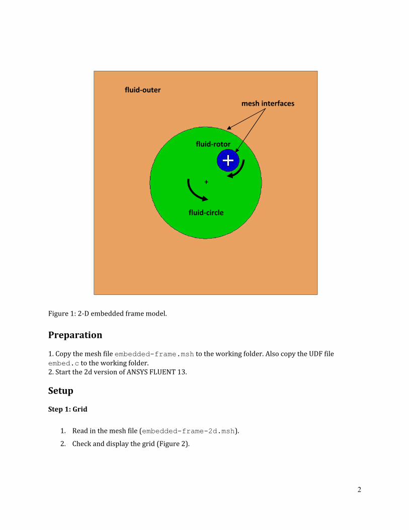
Note: Much of the background and set up has been repeated from the MRF tutorial in order to make this tutorial selfcontained. You can save some set up work by reusing the case file from the MRF tutorial. Prerequisites This tutorial assumes that you are familiar with the FLUENT interface and have a good understanding of basic setup and solution procedures. Some details not relevant to the setup will be omitted or only briefly mentioned. Problem Description This tutorial considers a simple 2‐D closed system as depicted in Figure 1. It consists of a cross‐shaped rotor domain (diameter = 0.1 m) which is offset from the center of a circular domain (diameter = 0.5 m) by 0.1 m in the x and y directions. The rotor is spinning clockwise at 2 rad/s. The circular domain, in turn, is centered within a square fluid domain which is bounded by impermeable walls. The circular domain is spinning counterclockwise at 1rad/s. The working fluid is water with a density of 1000 kg/m3 and viscosity of 0.001 kg/m‐s.
2
Figure 1: 2‐D embedded frame model. Preparation 1. Copy the mesh file embedded-frame.msh to the working folder. Also copy the UDF file embed.c to the working folder. 2. Start the 2d version of ANSYS FLUENT 13. Setup Step 1: Grid
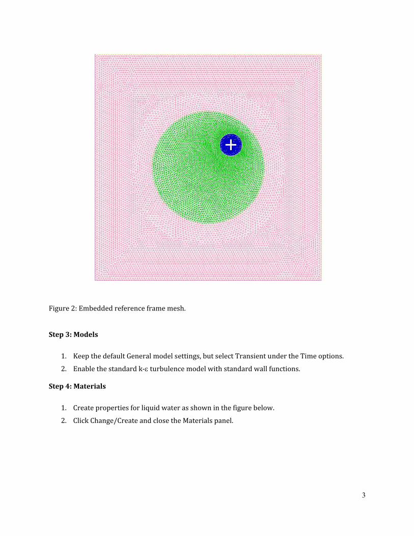
1. Keep the default General model settings, but select Transient under the Time options.
2. Enable the standard k‐ε turbulence model with standard wall functions. Step 4: Materials
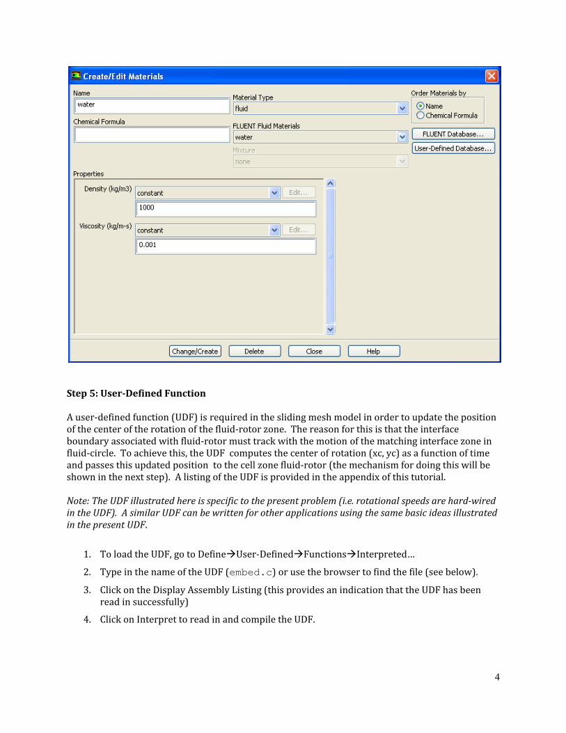
1. Create properties for liquid water as shown in the figure below.
2. Click Change/Create and close the Materials panel.
4
Step 5: UserDefined Function A user‐defined function (UDF) is required in the sliding mesh model in order to update the position of the center of the rotation of the fluid‐rotor zone. The reason for this is that the interface boundary associated with fluid‐rotor must track with the motion of the matching interface zone in fluid‐circle. To achieve this, the UDF computes the center of rotation (xc, yc) as a function of time and passes this updated position to the cell zone fluid‐rotor (the mechanism for doing this will be shown in the next step). A listing of the UDF is provided in the appendix of this tutorial. Note: The UDF illustrated here is specific to the present problem (i.e. rotational speeds are hardwired in the UDF). A similar UDF can be written for other applications using the same basic ideas illustrated in the present UDF.
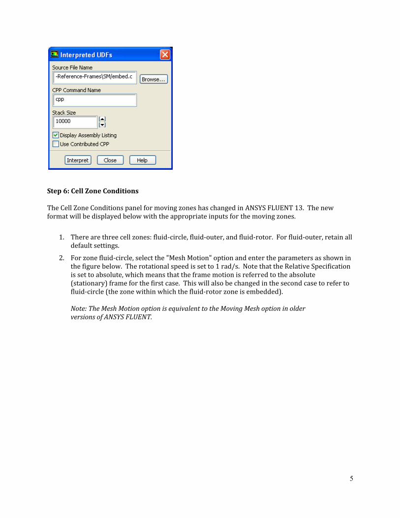
1. To load the UDF, go to Define User‐Defined Functions Interpreted…
2. Type in the name of the UDF (embed.c) or use the browser to find the file (see below).
3. Click on the Display Assembly Listing (this provides an indication that the UDF has been read in successfully)
4. Click on Interpret to read in and compile the UDF.
5
Step 6: Cell Zone Conditions The Cell Zone Conditions panel for moving zones has changed in ANSYS FLUENT 13. The new format will be displayed below with the appropriate inputs for the moving zones.
1. There are three cell zones: fluid‐circle, fluid‐outer, and fluid‐rotor. For fluid‐outer, retain all default settings.
2. For zone fluid‐circle, select the "Mesh Motion" option and enter the parameters as shown in the figure below. The rotational speed is set to 1 rad/s. Note that the Relative Specification is set to absolute, which means that the frame motion is referred to the absolute (stationary) frame for the first case. This will also be changed in the second case to refer to fluid‐circle (the zone within which the fluid‐rotor zone is embedded).
Note: The Mesh Motion option is equivalent to the Moving Mesh option in older versions of ANSYS FLUENT.
6
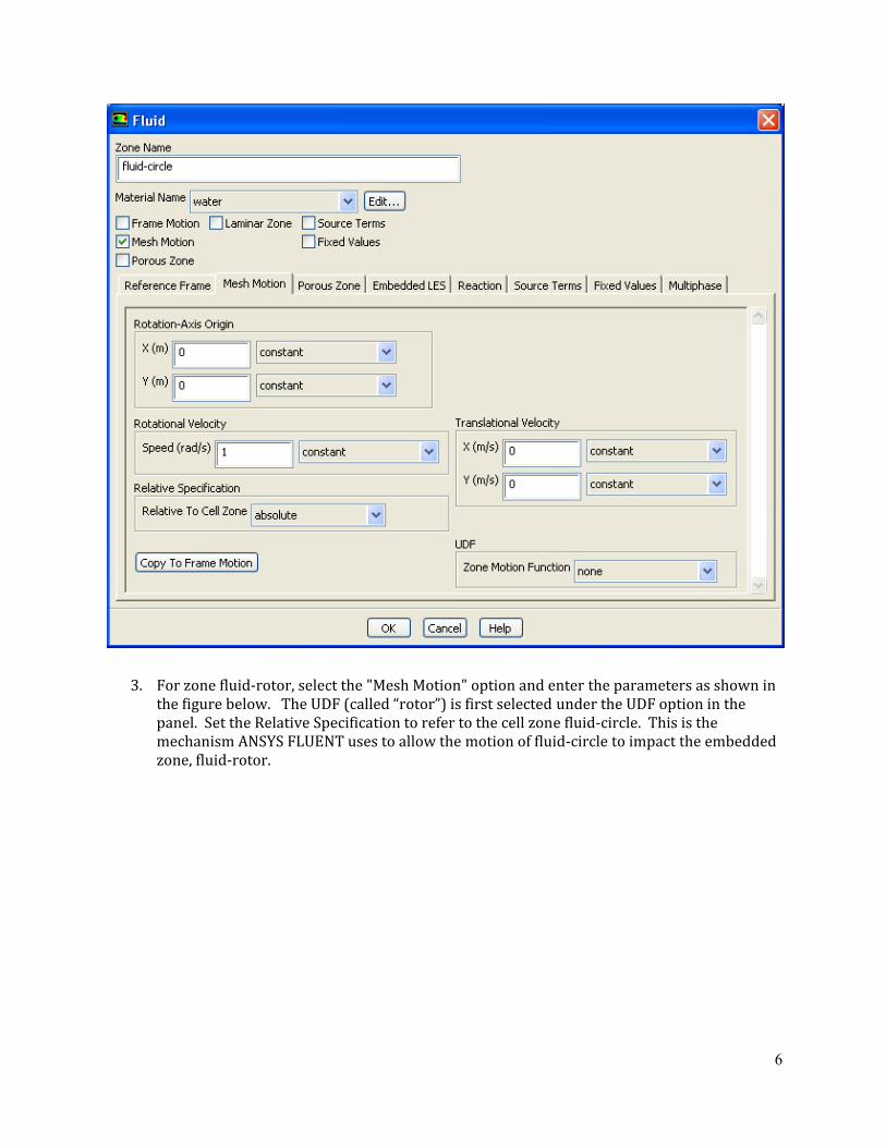
3. For zone fluid‐rotor, select the "Mesh Motion" option and enter the parameters as shown in the figure below. The UDF (called “rotor”) is first selected under the UDF option in the panel. Set the Relative Specification to refer to the cell zone fluid‐circle. This is the mechanism ANSYS FLUENT uses to allow the motion of fluid‐circle to impact the embedded zone, fluid‐rotor.
7
Step 6: Boundary Conditions
1. The only boundary conditions that need to be set are the outer boundary walls and the rotor walls. You can, in the present case, retain the defaults for these boundaries.
Step 7: Mesh Interfaces
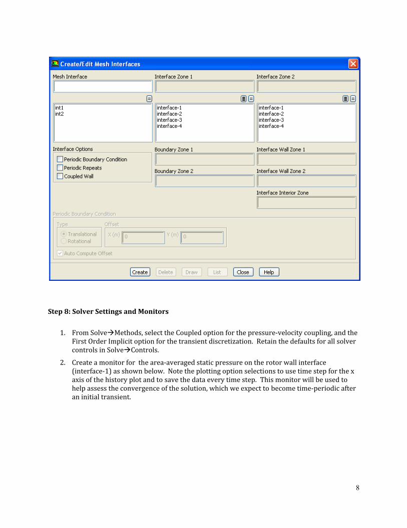
1. Open the Mesh Interfaces panel and create two interfaces: (1) mesh interface between fluid‐circle and fluid‐outer (using zones interface‐1 and interface‐2), and (2) mesh‐interface between fluid‐circle and fluid‐rotor (using zones interface‐3 and interface‐4). The panel is shown below.
8
Step 8: Solver Settings and Monitors
1. From Solve Methods, select the Coupled option for the pressure‐velocity coupling, and the First Order Implicit option for the transient discretization. Retain the defaults for all solver controls in Solve Controls.
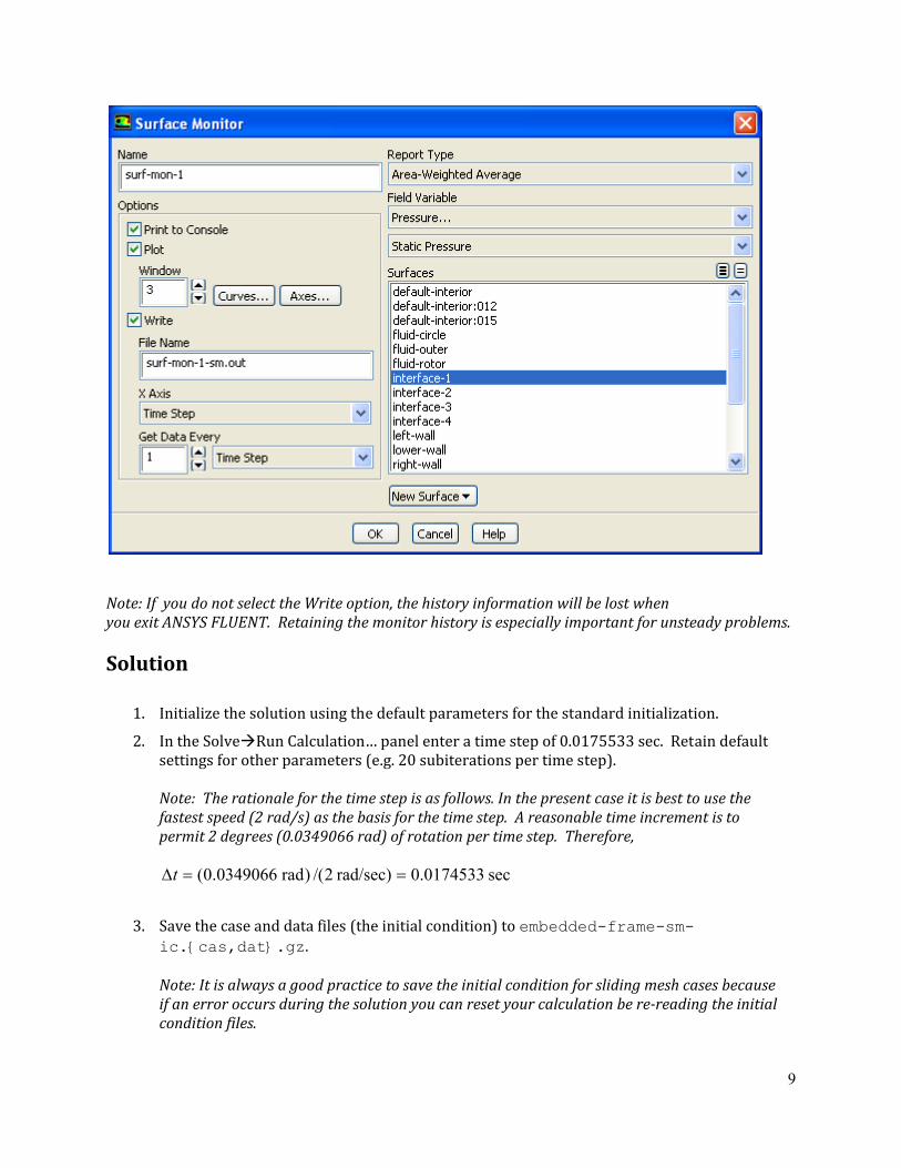
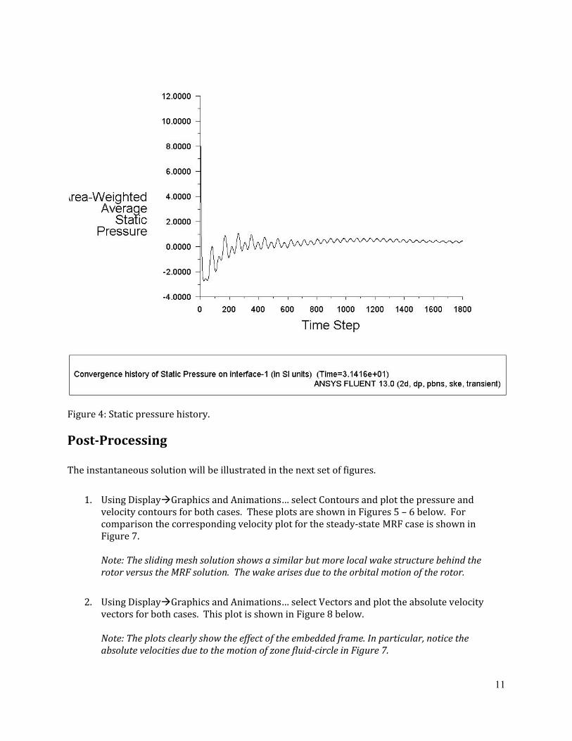
2. Create a monitor for the area‐averaged static pressure on the rotor wall interface (interface‐1) as shown below. Note the plotting option selections to use time step for the x axis of the history plot and to save the data every time step. This monitor will be used to help assess the convergence of the solution, which we expect to become time‐periodic after an initial transient.
9
Note: If you do not select the Write option, the history information will be lost when you exit ANSYS FLUENT. Retaining the monitor history is especially important for unsteady problems. Solution
1. Initialize the solution using the default parameters for the standard initialization.
2. In the Solve Run Calculation… panel enter a time step of 0.0175533 sec. Retain default settings for other parameters (e.g. 20 subiterations per time step).
Note: The rationale for the time step is as follows. In the present case it is best to use the fastest speed (2 rad/s) as the basis for the time step. A reasonable time increment is to permit 2 degrees (0.0349066 rad) of rotation per time step. Therefore,
sec 0.0174533rad/sec) 2/()rad 0349066.0( ==Δt
3. Save the case and data files (the initial condition) to embedded-frame-sm-ic.{cas,dat}.gz.
Note: It is always a good practice to save the initial condition for sliding mesh cases because if an error occurs during the solution you can reset your calculation be rereading the initial condition files.
10
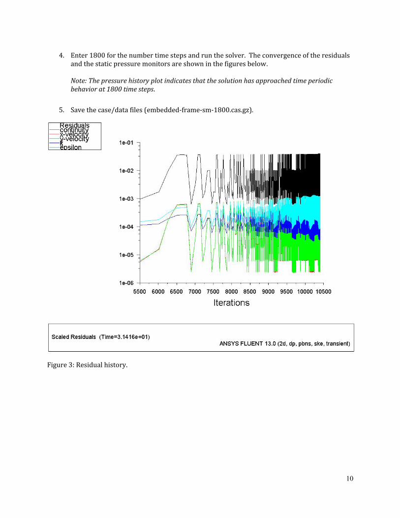
4. Enter 1800 for the number time steps and run the solver. The convergence of the residuals and the static pressure monitors are shown in the figures below.
Note: The pressure history plot indicates that the solution has approached time periodic behavior at 1800 time steps.
5. Save the case/data files (embedded‐frame‐sm‐1800.cas.gz).
Figure 3: Residual history.
11
Figure 4: Static pressure history. PostProcessing The instantaneous solution will be illustrated in the next set of figures.
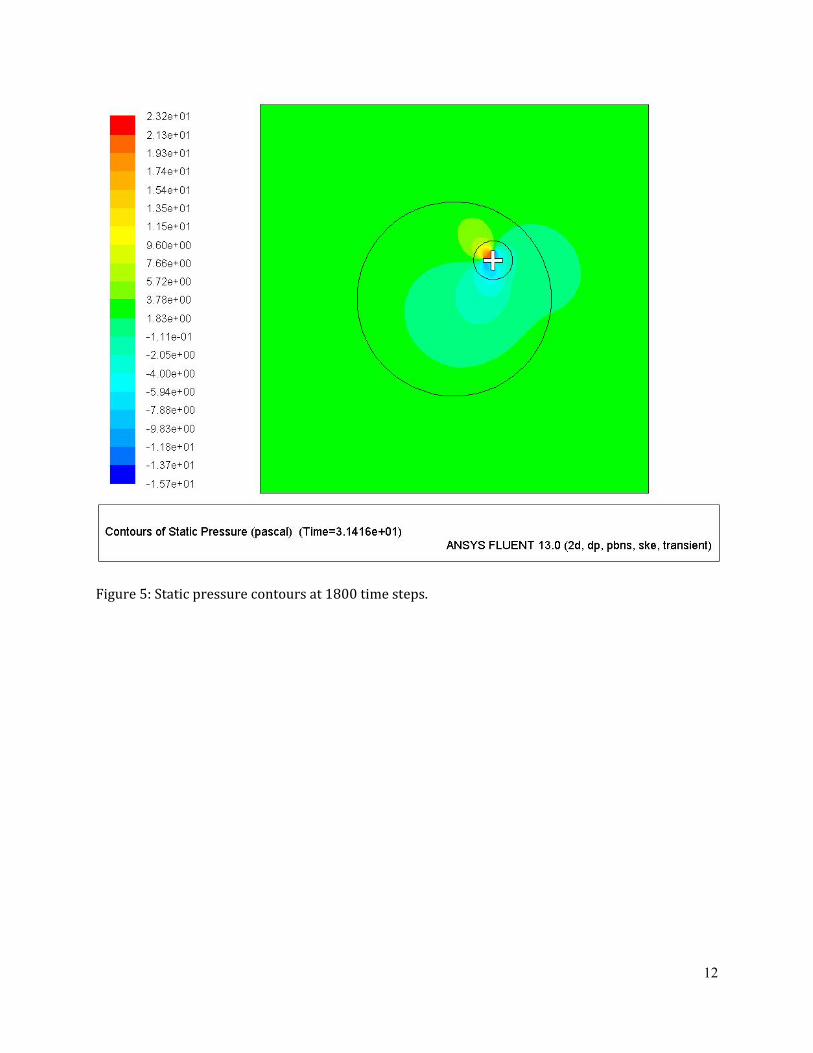
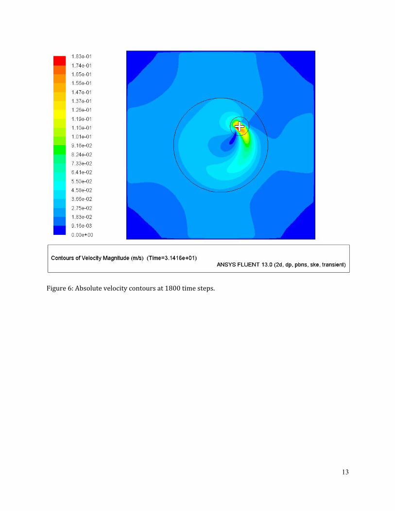
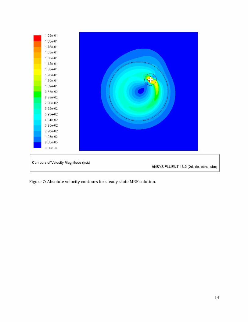
1. Using Display Graphics and Animations… select Contours and plot the pressure and velocity contours for both cases. These plots are shown in Figures 5 – 6 below. For comparison the corresponding velocity plot for the steady‐state MRF case is shown in Figure 7.
Note: The sliding mesh solution shows a similar but more local wake structure behind the rotor versus the MRF solution. The wake arises due to the orbital motion of the rotor.
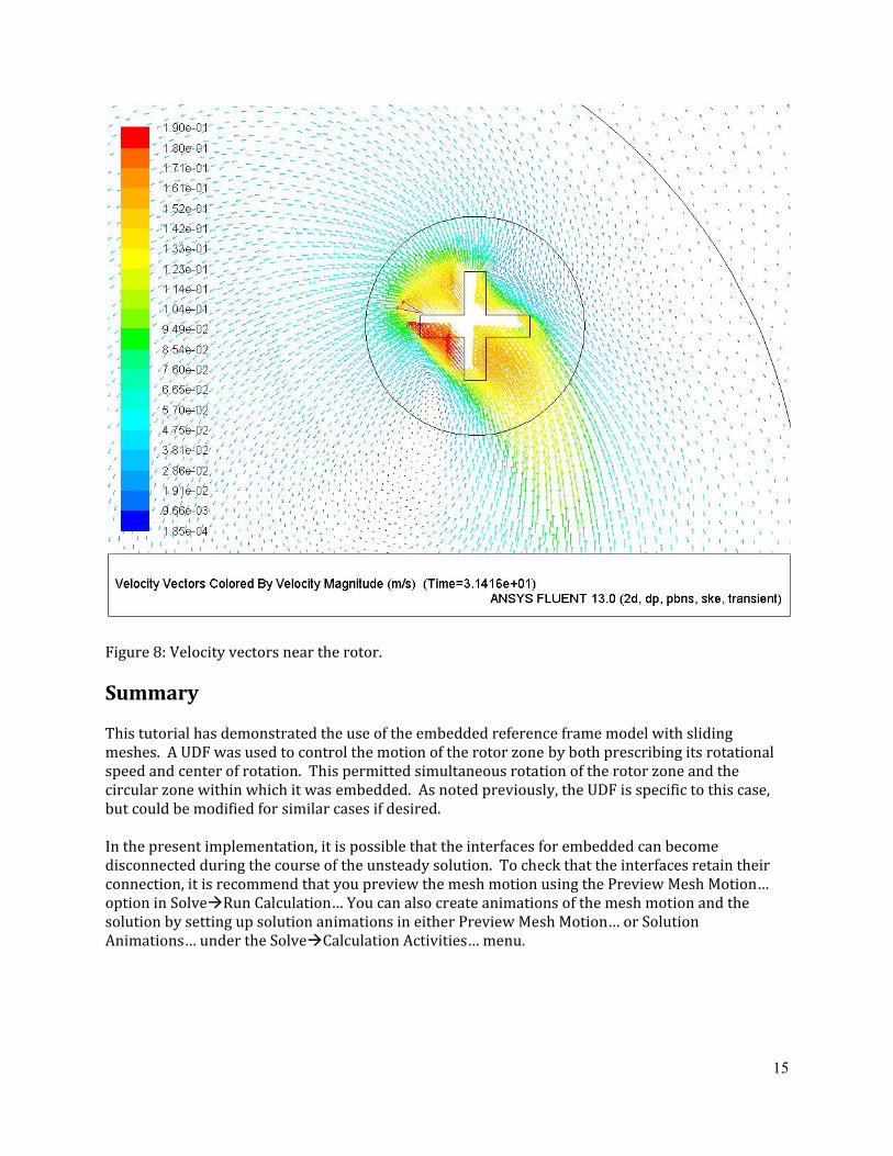
2. Using Display Graphics and Animations… select Vectors and plot the absolute velocity vectors for both cases. This plot is shown in Figure 8 below.
Note: The plots clearly show the effect of the embedded frame. In particular, notice the absolute velocities due to the motion of zone fluidcircle in Figure 7.
12
Figure 5: Static pressure contours at 1800 time steps.
13
Figure 6: Absolute velocity contours at 1800 time steps.
14
Figure 7: Absolute velocity contours for steady‐state MRF solution.
15
Figure 8: Velocity vectors near the rotor.
Summary This tutorial has demonstrated the use of the embedded reference frame model with sliding meshes. A UDF was used to control the motion of the rotor zone by both prescribing its rotational speed and center of rotation. This permitted simultaneous rotation of the rotor zone and the circular zone within which it was embedded. As noted previously, the UDF is specific to this case, but could be modified for similar cases if desired. In the present implementation, it is possible that the interfaces for embedded can become disconnected during the course of the unsteady solution. To check that the interfaces retain their connection, it is recommend that you preview the mesh motion using the Preview Mesh Motion… option in Solve Run Calculation… You can also create animations of the mesh motion and the solution by setting up solution animations in either Preview Mesh Motion… or Solution Animations… under the Solve Calculation Activities… menu.
16
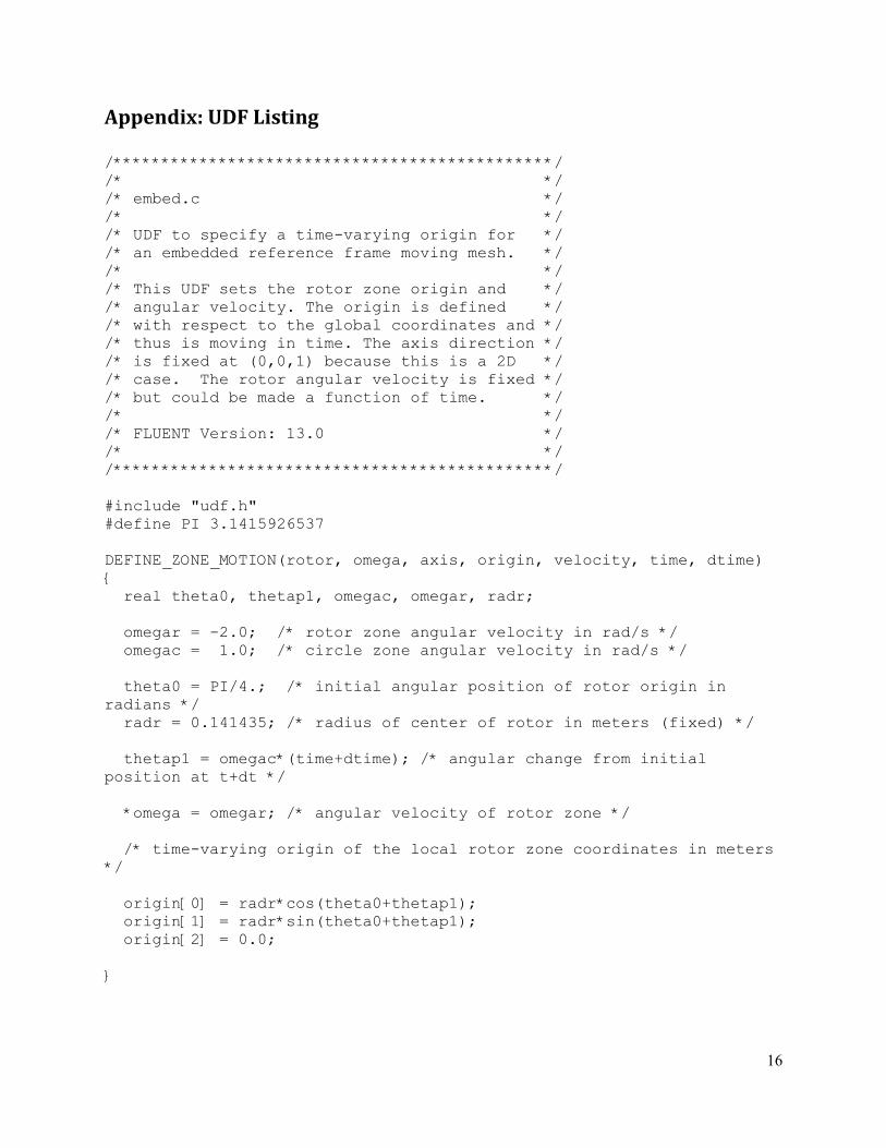
Appendix: UDF Listing /**********************************************/ /* */ /* embed.c */ /* */ /* UDF to specify a time-varying origin for */ /* an embedded reference frame moving mesh. */ /* */ /* This UDF sets the rotor zone origin and */ /* angular velocity. The origin is defined */ /* with respect to the global coordinates and */ /* thus is moving in time. The axis direction */ /* is fixed at (0,0,1) because this is a 2D */ /* case. The rotor angular velocity is fixed */ /* but could be made a function of time. */ /* */ /* FLUENT Version: 13.0 */ /* */ /**********************************************/ #include "udf.h" #define PI 3.1415926537 DEFINE_ZONE_MOTION(rotor, omega, axis, origin, velocity, time, dtime) { real theta0, thetap1, omegac, omegar, radr; omegar = -2.0; /* rotor zone angular velocity in rad/s */ omegac = 1.0; /* circle zone angular velocity in rad/s */ theta0 = PI/4.; /* initial angular position of rotor origin in radians */ radr = 0.141435; /* radius of center of rotor in meters (fixed) */ thetap1 = omegac*(time+dtime); /* angular change from initial position at t+dt */ *omega = omegar; /* angular velocity of rotor zone */ /* time-varying origin of the local rotor zone coordinates in meters */ origin[0] = radr*cos(theta0+thetap1); origin[1] = radr*sin(theta0+thetap1); origin[2] = 0.0; }