187
Several perspectives and solutions on Bayesian testing of hypotheses Christian P. Robert Universit´ e Paris-Dauphine, Paris & University of Warwick, Coventry
| Date post: | 29-Jul-2015 |
| Category: |
Science |
| Upload: | christian-robert |
| View: | 2,736 times |
| Download: | 1 times |

Several perspectives and solutions on Bayesiantesting of hypotheses
Christian P. RobertUniversite Paris-Dauphine, Paris & University of Warwick, Coventry

Outline
Significance tests: one new parameter
Noninformative solutions
Jeffreys-Lindley paradox
Deviance (information criterion)
Testing under incomplete information
Testing via mixtures

“Significance tests: one new parameter”
Significance tests: one new parameterBayesian testsBayes factorsImproper priors for testsConclusion
Noninformative solutions
Jeffreys-Lindley paradox
Deviance (information criterion)
Testing under incomplete information
Testing via mixtures

Fundamental setting
Is the new parameter supported by the observations or isany variation expressible by it better interpreted asrandom? Thus we must set two hypotheses forcomparison, the more complicated having the smallerinitial probability (Jeffreys, ToP, V, §5.0)
...compare a specially suggested value of a newparameter, often 0 [q], with the aggregate of otherpossible values [q′]. We shall call q the null hypothesisand q′ the alternative hypothesis [and] we must take
P(q|H) = P(q′|H) = 1/2 .

Construction of Bayes tests
Definition (Test)
Given an hypothesis H0 : θ ∈ Θ0 on the parameter θ ∈ Θ0 of astatistical model, a test is a statistical procedure that takes itsvalues in {0, 1}.
Type–one and type–two errors
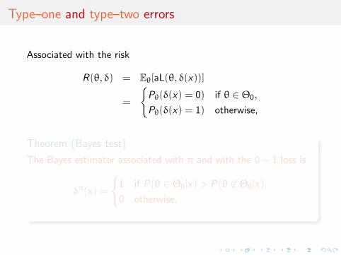
Associated with the risk
R(θ, δ) = Eθ[aL(θ, δ(x))]
=
{Pθ(δ(x) = 0) if θ ∈ Θ0,
Pθ(δ(x) = 1) otherwise,
Theorem (Bayes test)
The Bayes estimator associated with π and with the 0 − 1 loss is
δπ(x) =
{1 if P(θ ∈ Θ0|x) > P(θ 6∈ Θ0|x),
0 otherwise,
Type–one and type–two errors
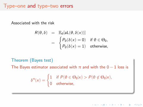
Associated with the risk
R(θ, δ) = Eθ[aL(θ, δ(x))]
=
{Pθ(δ(x) = 0) if θ ∈ Θ0,
Pθ(δ(x) = 1) otherwise,
Theorem (Bayes test)
The Bayes estimator associated with π and with the 0 − 1 loss is
δπ(x) =
{1 if P(θ ∈ Θ0|x) > P(θ 6∈ Θ0|x),
0 otherwise,

Jeffreys’ example (§5.0)
Testing whether the mean α of a normal observation is zero:
P(q|aH) ∝ exp
(−
a2
2s2
)P(q′dα|aH) ∝ exp
(−(a − α)2
2s2
)f (α)dα
P(q′|aH) ∝∫
exp
(−(a − α)2
2s2
)f (α)dα

A (small) point of contention
Jeffreys asserts
Suppose that there is one old parameter α; the newparameter is β and is 0 on q. In q′ we could replace α byα′, any function of α and β: but to make it explicit thatq′ reduces to q when β = 0 we shall require that α′ = αwhen β = 0 (V, §5.0).
This amounts to assume identical parameters in both models, acontroversial principle for model choice or at the very best to makeα and β dependent a priori, a choice contradicted by the nextparagraph in ToP
Orthogonal parameters
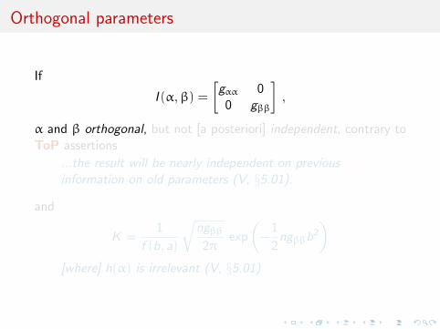
If
I (α,β) =
[gαα 0
0 gββ
],
α and β orthogonal, but not [a posteriori] independent, contrary toToP assertions
...the result will be nearly independent on previousinformation on old parameters (V, §5.01).
and
K =1
f (b, a)
√ngββ2π
exp
(−
1
2ngββb2
)[where] h(α) is irrelevant (V, §5.01)

Orthogonal parameters
If
I (α,β) =
[gαα 0
0 gββ
],
α and β orthogonal, but not [a posteriori] independent, contrary toToP assertions
...the result will be nearly independent on previousinformation on old parameters (V, §5.01).
and
K =1
f (b, a)
√ngββ2π
exp
(−
1
2ngββb2
)[where] h(α) is irrelevant (V, §5.01)

Acknowledgement in ToP
In practice it is rather unusual for a set of parameters toarise in such a way that each can be treated as irrelevantto the presence of any other. More usual cases are (...)where some parameters are so closely associated that onecould hardly occur without the others (V, §5.04).

Generalisation
Theorem (Optimal Bayes decision)
Under the 0 − 1 loss function
L(θ, d) =
0 if d = IΘ0(θ)
a0 if d = 1 and θ 6∈ Θ0
a1 if d = 0 and θ ∈ Θ0
the Bayes procedure is
δπ(x) =
{1 if Prπ(θ ∈ Θ0|x) > a0/(a0 + a1)
0 otherwise

Generalisation
Theorem (Optimal Bayes decision)
Under the 0 − 1 loss function
L(θ, d) =
0 if d = IΘ0(θ)
a0 if d = 1 and θ 6∈ Θ0
a1 if d = 0 and θ ∈ Θ0
the Bayes procedure is
δπ(x) =
{1 if Prπ(θ ∈ Θ0|x) > a0/(a0 + a1)
0 otherwise

Bound comparison
Determination of a0/a1 depends on consequences of “wrongdecision” under both circumstancesOften difficult to assess in practice and replacement with “golden”default bounds like .05, biased towards H0

Bound comparison
Determination of a0/a1 depends on consequences of “wrongdecision” under both circumstancesOften difficult to assess in practice and replacement with “golden”default bounds like .05, biased towards H0
A function of posterior probabilities
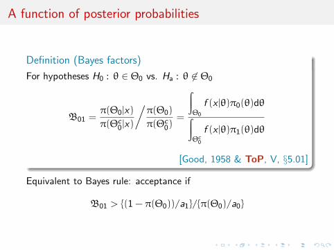
Definition (Bayes factors)
For hypotheses H0 : θ ∈ Θ0 vs. Ha : θ 6∈ Θ0
B01 =π(Θ0|x)
π(Θc0|x)
/π(Θ0)
π(Θc0)
=
∫Θ0
f (x |θ)π0(θ)dθ∫Θc
0
f (x |θ)π1(θ)dθ
[Good, 1958 & ToP, V, §5.01]
Equivalent to Bayes rule: acceptance if
B01 > {(1 − π(Θ0))/a1}/{π(Θ0)/a0}

Self-contained concept
Outside decision-theoretic environment:
I eliminates choice of π(Θ0)
I but depends on the choice of (π0,π1)
I Bayesian/marginal equivalent to the likelihood ratioI Jeffreys’ scale of evidence:
I if log10(Bπ10) between 0 and 0.5, evidence against H0 weak,
I if log10(Bπ10) 0.5 and 1, evidence substantial,
I if log10(Bπ10) 1 and 2, evidence strong and
I if log10(Bπ10) above 2, evidence decisive

A major modification
When the null hypothesis is supported by a set of measure 0against Lebesgue measure, π(Θ0) = 0 for an absolutely continuousprior distribution
[End of the story?!]
Suppose we are considering whether a location parameterα is 0. The estimation prior probability for it is uniformand we should have to take f (α) = 0 and K [= B10]would always be infinite (V, §5.02)

Point null refurbishment
Requirement
Defined prior distributions under both assumptions,
π0(θ) ∝ π(θ)IΘ0(θ), π1(θ) ∝ π(θ)IΘ1(θ),
(under the standard dominating measures on Θ0 and Θ1)
Using the prior probabilities π(Θ0) = ρ0 and π(Θ1) = ρ1,
π(θ) = ρ0π0(θ) + ρ1π1(θ).
Note If Θ0 = {θ0}, π0 is the Dirac mass in θ0
Point null hypotheses
Particular case H0 : θ = θ0Take ρ0 = Prπ(θ = θ0) and g1 prior density under Ha.Posterior probability of H0
π(Θ0|x) =f (x |θ0)ρ0∫
f (x |θ)π(θ) dθ=
f (x |θ0)ρ0f (x |θ0)ρ0 + (1 − ρ0)m1(x)
and marginal under Ha
m1(x) =
∫Θ1
f (x |θ)g1(θ) dθ.
Point null hypotheses
Particular case H0 : θ = θ0Take ρ0 = Prπ(θ = θ0) and g1 prior density under Ha.Posterior probability of H0
π(Θ0|x) =f (x |θ0)ρ0∫
f (x |θ)π(θ) dθ=
f (x |θ0)ρ0f (x |θ0)ρ0 + (1 − ρ0)m1(x)
and marginal under Ha
m1(x) =
∫Θ1
f (x |θ)g1(θ) dθ.
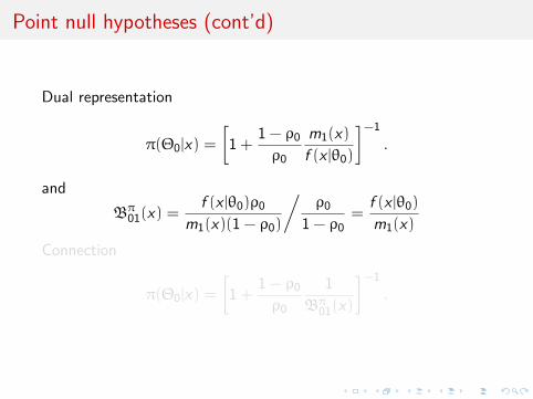
Point null hypotheses (cont’d)
Dual representation
π(Θ0|x) =
[1 +
1 − ρ0ρ0
m1(x)
f (x |θ0)
]−1
.
and
Bπ01(x) =
f (x |θ0)ρ0m1(x)(1 − ρ0)
/ρ0
1 − ρ0=
f (x |θ0)
m1(x)
Connection
π(Θ0|x) =
[1 +
1 − ρ0ρ0
1
Bπ01(x)
]−1
.

Point null hypotheses (cont’d)
Dual representation
π(Θ0|x) =
[1 +
1 − ρ0ρ0
m1(x)
f (x |θ0)
]−1
.
and
Bπ01(x) =
f (x |θ0)ρ0m1(x)(1 − ρ0)
/ρ0
1 − ρ0=
f (x |θ0)
m1(x)
Connection
π(Θ0|x) =
[1 +
1 − ρ0ρ0
1
Bπ01(x)
]−1
.

A further difficulty
Improper priors are not allowed here
If ∫Θ1
π1(dθ1) =∞ or
∫Θ2
π2(dθ2) =∞then π1 or π2 cannot be coherently normalised while thenormalisation matters in the Bayes factor remember Bayes factor?

A further difficulty
Improper priors are not allowed here
If ∫Θ1
π1(dθ1) =∞ or
∫Θ2
π2(dθ2) =∞then π1 or π2 cannot be coherently normalised while thenormalisation matters in the Bayes factor remember Bayes factor?

ToP unaware of the problem?
A. Not entirely, as improper priors keep being used on nuisanceparameters
Example of testing for a zero normal mean:
If σ is the standard error and λ the true value, λ is 0 onq. We want a suitable form for its prior on q′. (...) Thenwe should take
P(qdσ|H) ∝ dσ/σ
P(q′dσdλ|H) ∝ f
(λ
σ
)dσ/σdλ/λ
where f [is a true density] (V, §5.2).
Fallacy of the “same” σ!

Not enought information
If s ′ = 0 [!!!], then [for σ = |x |/τ, λ = σv]
P(q|θH) ∝∫∞0
(τ
|x |
)n
exp
(−
1
2nτ2)
dτ
τ,
P(q′|θH) ∝∫∞0
dτ
τ
∫∞−∞
(τ
|x |
)n
f (v) exp
(−
1
2n(v − τ)2
).
If n = 1 and f (v) is any even [density],
P(q′|θH) ∝ 1
2
√2π
|x |and P(q|θH) ∝ 1
2
√2π
|x |
and therefore K = 1 (V, §5.2).

Strange constraints
If n > 2, the condition that K = 0 for s ′ = 0, x 6= 0 isequivalent to ∫∞
0f (v)vn−1dv =∞ .
The function satisfying this condition for [all] n is
f (v) =1
π(1 + v2)
This is the prior recommended by Jeffreys hereafter.But, first, many other families of densities satisfy this constraintand a scale of 1 cannot be universal!Second, s ′ = 0 is a zero probability event...
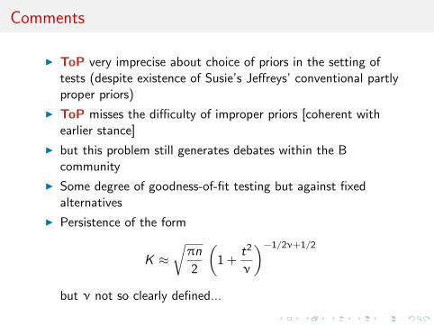
Comments
I ToP very imprecise about choice of priors in the setting oftests (despite existence of Susie’s Jeffreys’ conventional partlyproper priors)
I ToP misses the difficulty of improper priors [coherent withearlier stance]
I but this problem still generates debates within the Bcommunity
I Some degree of goodness-of-fit testing but against fixedalternatives
I Persistence of the form
K ≈√πn
2
(1 +
t2
ν
)−1/2ν+1/2
but ν not so clearly defined...

Noninformative proposals
Significance tests: one new parameter
Noninformative solutionsPseudo-Bayes factorsIntrinsic priors
Jeffreys-Lindley paradox
Deviance (information criterion)
Testing under incomplete information
Testing via mixtures

Vague proper priors are not the solution
Taking a proper prior and take a “very large” variance (e.g.,BUGS) will most often result in an undefined or ill-defined limit
Example (Lindley’s paradox)
If testing H0 : θ = 0 when observing x ∼ N(θ, 1), under a normalN(0,α) prior π1(θ),
B01(x)α−→∞−→ 0

Vague proper priors are not the solution
Taking a proper prior and take a “very large” variance (e.g.,BUGS) will most often result in an undefined or ill-defined limit
Example (Lindley’s paradox)
If testing H0 : θ = 0 when observing x ∼ N(θ, 1), under a normalN(0,α) prior π1(θ),
B01(x)α−→∞−→ 0

Vague proper priors are not the solution
Taking a proper prior and take a “very large” variance (e.g.,BUGS) will most often result in an undefined or ill-defined limit
Example (Lindley’s paradox)
If testing H0 : θ = 0 when observing x ∼ N(θ, 1), under a normalN(0,α) prior π1(θ),
B01(x)α−→∞−→ 0

Vague proper priors are not the solution (cont’d)
Example (Poisson versus Negative binomial (4))
B12 =
∫10
λα+x−1
x !e−λβdλ
1
M
∑m
x
m − x + 1
βα
Γ(α)
if λ ∼ Ga(α,β)
=Γ(α+ x)
x ! Γ(α)β−x
/1
M
∑m
x
m − x + 1
=(x + α− 1) · · ·α
x(x − 1) · · · 1β−x
/1
M
∑m
x
m − x + 1
depends on choice of α(β) or β(α) −→ 0

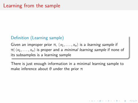
Learning from the sample
Definition (Learning sample)
Given an improper prior π, (x1, . . . , xn) is a learning sample ifπ(·|x1, . . . , xn) is proper and a minimal learning sample if none ofits subsamples is a learning sample
There is just enough information in a minimal learning sample tomake inference about θ under the prior π
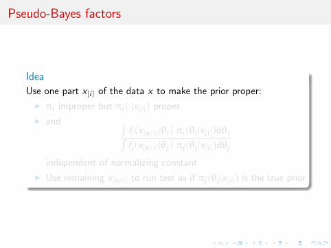
Pseudo-Bayes factors
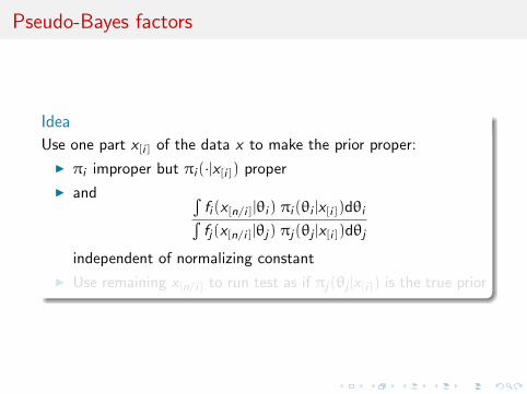
Idea
Use one part x[i] of the data x to make the prior proper:
I πi improper but πi (·|x[i]) proper
I and ∫fi (x[n/i]|θi ) πi (θi |x[i])dθi∫fj(x[n/i]|θj) πj(θj |x[i])dθj
independent of normalizing constant
I Use remaining x[n/i] to run test as if πj(θj |x[i]) is the true prior
Pseudo-Bayes factors
Idea
Use one part x[i] of the data x to make the prior proper:
I πi improper but πi (·|x[i]) proper
I and ∫fi (x[n/i]|θi ) πi (θi |x[i])dθi∫fj(x[n/i]|θj) πj(θj |x[i])dθj
independent of normalizing constant
I Use remaining x[n/i] to run test as if πj(θj |x[i]) is the true prior

Pseudo-Bayes factors
Idea
Use one part x[i] of the data x to make the prior proper:
I πi improper but πi (·|x[i]) proper
I and ∫fi (x[n/i]|θi ) πi (θi |x[i])dθi∫fj(x[n/i]|θj) πj(θj |x[i])dθj
independent of normalizing constant
I Use remaining x[n/i] to run test as if πj(θj |x[i]) is the true prior

Motivation
I Provides a working principle for improper priors
I Gather enough information from data to achieve properness
I and use this properness to run the test on remaining data
I does not use x twice as in Aitkin’s (1991)

Motivation
I Provides a working principle for improper priors
I Gather enough information from data to achieve properness
I and use this properness to run the test on remaining data
I does not use x twice as in Aitkin’s (1991)

Motivation
I Provides a working principle for improper priors
I Gather enough information from data to achieve properness
I and use this properness to run the test on remaining data
I does not use x twice as in Aitkin’s (1991)
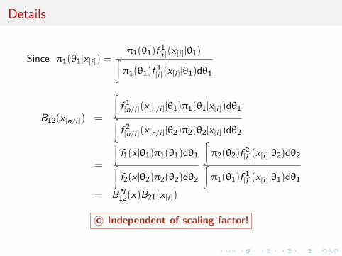
Details
Since π1(θ1|x[i]) =π1(θ1)f
1[i](x[i]|θ1)∫
π1(θ1)f1[i](x[i]|θ1)dθ1
B12(x[n/i]) =
∫f 1[n/i](x[n/i]|θ1)π1(θ1|x[i])dθ1∫
f 2[n/i](x[n/i]|θ2)π2(θ2|x[i])dθ2
=
∫f1(x |θ1)π1(θ1)dθ1∫f2(x |θ2)π2(θ2)dθ2
∫π2(θ2)f
2[i](x[i]|θ2)dθ2∫
π1(θ1)f1[i](x[i]|θ1)dθ1
= BN12(x)B21(x[i])
c© Independent of scaling factor!

Unexpected problems!
I depends on the choice of x[i]I many ways of combining pseudo-Bayes factors
I AIBF = BNji
1
L
∑`
Bij(x[`])
I MIBF = BNji med[Bij(x[`])]
I GIBF = BNji exp
1
L
∑`
log Bij(x[`])
I not often an exact Bayes factor
I and thus lacking inner coherence
B12 6= B10B02 and B01 6= 1/B10 .
[Berger & Pericchi, 1996]

Unexpec’d problems (cont’d)
Example (Mixtures)
There is no sample size that proper-ises improper priors, except if atraining sample is allocated to each componentReason If
x1, . . . , xn ∼
k∑i=1
pi f (x |θi )
and
π(θ) =∏i
πi (θi ) with
∫πi (θi )dθi = +∞ ,
the posterior is never defined, because
Pr(“no observation from f (·|θi )”) = (1 − pi )n
Intrinsic priors
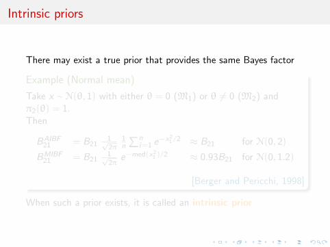
There may exist a true prior that provides the same Bayes factor
Example (Normal mean)
Take x ∼ N(θ, 1) with either θ = 0 (M1) or θ 6= 0 (M2) andπ2(θ) = 1.Then
BAIBF21 = B21
1√2π
1n
∑ni=1 e−x21 /2 ≈ B21 for N(0, 2)
BMIBF21 = B21
1√2π
e−med(x21 )/2 ≈ 0.93B21 for N(0, 1.2)
[Berger and Pericchi, 1998]
When such a prior exists, it is called an intrinsic prior

Intrinsic priors
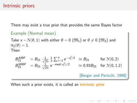
There may exist a true prior that provides the same Bayes factor
Example (Normal mean)
Take x ∼ N(θ, 1) with either θ = 0 (M1) or θ 6= 0 (M2) andπ2(θ) = 1.Then
BAIBF21 = B21
1√2π
1n
∑ni=1 e−x21 /2 ≈ B21 for N(0, 2)
BMIBF21 = B21
1√2π
e−med(x21 )/2 ≈ 0.93B21 for N(0, 1.2)
[Berger and Pericchi, 1998]
When such a prior exists, it is called an intrinsic prior
Intrinsic priors
There may exist a true prior that provides the same Bayes factor
Example (Normal mean)
Take x ∼ N(θ, 1) with either θ = 0 (M1) or θ 6= 0 (M2) andπ2(θ) = 1.Then
BAIBF21 = B21
1√2π
1n
∑ni=1 e−x21 /2 ≈ B21 for N(0, 2)
BMIBF21 = B21
1√2π
e−med(x21 )/2 ≈ 0.93B21 for N(0, 1.2)
[Berger and Pericchi, 1998]
When such a prior exists, it is called an intrinsic prior
Intrinsic priors (cont’d)
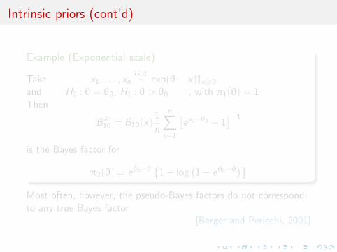
Example (Exponential scale)
Take x1, . . . , xni.i.d.∼ exp(θ− x)Ix>θ
and H0 : θ = θ0, H1 : θ > θ0 , with π1(θ) = 1Then
BA10 = B10(x)
1
n
n∑i=1
[exi−θ0 − 1
]−1
is the Bayes factor for
π2(θ) = eθ0−θ{
1 − log(1 − eθ0−θ
)}Most often, however, the pseudo-Bayes factors do not correspondto any true Bayes factor
[Berger and Pericchi, 2001]
Intrinsic priors (cont’d)
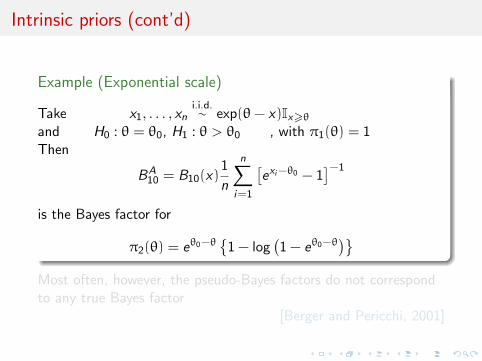
Example (Exponential scale)
Take x1, . . . , xni.i.d.∼ exp(θ− x)Ix>θ
and H0 : θ = θ0, H1 : θ > θ0 , with π1(θ) = 1Then
BA10 = B10(x)
1
n
n∑i=1
[exi−θ0 − 1
]−1
is the Bayes factor for
π2(θ) = eθ0−θ{
1 − log(1 − eθ0−θ
)}Most often, however, the pseudo-Bayes factors do not correspondto any true Bayes factor
[Berger and Pericchi, 2001]

Intrinsic priors (cont’d)
Example (Exponential scale)
Take x1, . . . , xni.i.d.∼ exp(θ− x)Ix>θ
and H0 : θ = θ0, H1 : θ > θ0 , with π1(θ) = 1Then
BA10 = B10(x)
1
n
n∑i=1
[exi−θ0 − 1
]−1
is the Bayes factor for
π2(θ) = eθ0−θ{
1 − log(1 − eθ0−θ
)}Most often, however, the pseudo-Bayes factors do not correspondto any true Bayes factor
[Berger and Pericchi, 2001]

Fractional Bayes factor
Idea
use directly the likelihood to separate training sample from testingsample
BF12 = B12(x)
∫Lb2(θ2)π2(θ2)dθ2∫
Lb1(θ1)π1(θ1)dθ1
[O’Hagan, 1995]
Proportion b of the sample used to gain proper-ness

Fractional Bayes factor
Idea
use directly the likelihood to separate training sample from testingsample
BF12 = B12(x)
∫Lb2(θ2)π2(θ2)dθ2∫
Lb1(θ1)π1(θ1)dθ1
[O’Hagan, 1995]
Proportion b of the sample used to gain proper-ness
Fractional Bayes factor (cont’d)
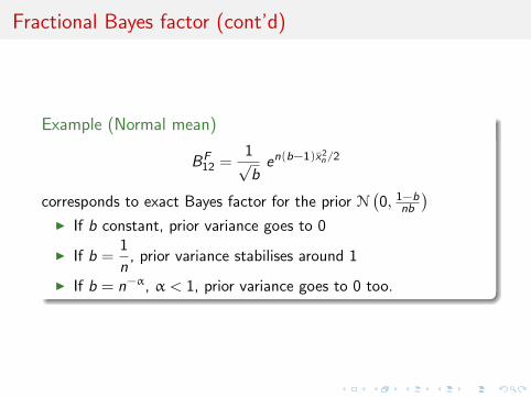
Example (Normal mean)
BF12 =
1√b
en(b−1)x2n/2
corresponds to exact Bayes factor for the prior N(0, 1−b
nb
)I If b constant, prior variance goes to 0
I If b =1
n, prior variance stabilises around 1
I If b = n−α, α < 1, prior variance goes to 0 too.

Jeffreys–Lindley paradox
Significance tests: one new parameter
Noninformative solutions
Jeffreys-Lindley paradoxLindley’s paradoxdual versions of the paradoxBayesian resolutions
Deviance (information criterion)
Testing under incomplete information
Testing via mixtures

Lindley’s paradox
In a normal mean testing problem,
xn ∼ N(θ,σ2/n) , H0 : θ = θ0 ,
under Jeffreys prior, θ ∼ N(θ0,σ2), the Bayes factor
B01(tn) = (1 + n)1/2 exp(−nt2n/2[1 + n]
),
where tn =√
n|xn − θ0|/σ, satisfies
B01(tn)n−→∞−→ ∞
[assuming a fixed tn][Lindley, 1957]

Lindley’s paradox
Often dubbed Jeffreys–Lindley paradox...
In terms of
t =√
n − 1x/s ′, ν = n−1
K ∼
√πν
2
(1 +
t2
ν
)−1/2ν+1/2
.
(...) The variation of K with tis much more important thanthe variation with ν (Jeffreys,V, §5.2).

Two versions of the paradox
“the weight of Lindley’s paradoxical result (...) burdensproponents of the Bayesian practice”.
[Lad, 2003]
I official version, opposing frequentist and Bayesian assessments[Lindley, 1957]
I intra-Bayesian version, blaming vague and improper priors forthe Bayes factor misbehaviour:if π1(·|σ) depends on a scale parameter σ, it is often the casethat
B01(x)σ−→∞−→ +∞
for a given x , meaning H0 is always accepted[Robert, 1992, 2013]
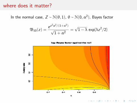
where does it matter?
In the normal case, Z ∼ N(θ, 1), θ ∼ N(0,α2), Bayes factor
B10(z) =ez
2α2/(1+α2)
√1 + α2
=√
1 − λ exp{λz2/2}
Evacuation of the first version
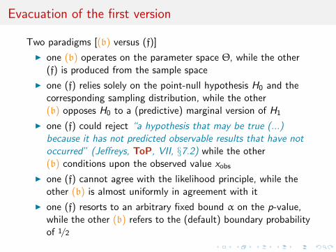
Two paradigms [(b) versus (f)]
I one (b) operates on the parameter space Θ, while the other(f) is produced from the sample space
I one (f) relies solely on the point-null hypothesis H0 and thecorresponding sampling distribution, while the other(b) opposes H0 to a (predictive) marginal version of H1
I one (f) could reject “a hypothesis that may be true (...)because it has not predicted observable results that have notoccurred” (Jeffreys, ToP, VII, §7.2) while the other(b) conditions upon the observed value xobs
I one (f) cannot agree with the likelihood principle, while theother (b) is almost uniformly in agreement with it
I one (f) resorts to an arbitrary fixed bound α on the p-value,while the other (b) refers to the (default) boundary probabilityof 1/2

More arguments on the first version
I observing a constant tn as n increases is of limited interest:under H0 tn has limiting N(0, 1) distribution, while, under H1
tn a.s. converges to ∞I behaviour that remains entirely compatible with the
consistency of the Bayes factor, which a.s. converges either to0 or ∞, depending on which hypothesis is true.
Consequent subsequent literature (e.g., Berger & Sellke, 1987;Bayarri & Berger, 2004) has since then shown how divergent thosetwo approaches could be (to the point of being asymptoticallyincompatible).

Nothing’s wrong with the second version
I n, prior’s scale factor: prior variance n times larger than theobservation variance and when n goes to ∞, Bayes factorgoes to ∞ no matter what the observation is
I n becomes what Lindley (1957) calls “a measure of lack ofconviction about the null hypothesis”
I when prior diffuseness under H1 increases, only relevantinformation becomes that θ could be equal to θ0, and thisoverwhelms any evidence to the contrary contained in the data
I mass of the prior distribution in the vicinity of any fixedneighbourhood of the null hypothesis vanishes to zero underH1
c© deep coherence in the outcome: being indecisive aboutthe alternative hypothesis means we should not chose it

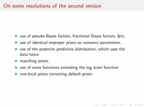
On some resolutions of the second version
I use of pseudo-Bayes factors, fractional Bayes factors, &tc,which lacks complete proper Bayesian justification
[Berger & Pericchi, 2001]
I use of identical improper priors on nuisance parameters,
I use of the posterior predictive distribution,
I matching priors,
I use of score functions extending the log score function
I non-local priors correcting default priors

On some resolutions of the second version
I use of pseudo-Bayes factors, fractional Bayes factors, &tc,
I use of identical improper priors on nuisance parameters, anotion already entertained by Jeffreys
[Berger et al., 1998; Marin & Robert, 2013]
I use of the posterior predictive distribution,
I matching priors,
I use of score functions extending the log score function
I non-local priors correcting default priors

On some resolutions of the second version
I use of pseudo-Bayes factors, fractional Bayes factors, &tc,
I use of identical improper priors on nuisance parameters,
I Peche de jeunesse: equating the values of the prior densitiesat the point-null value θ0,
ρ0 = (1 − ρ0)π1(θ0)
[Robert, 1993]
I use of the posterior predictive distribution,
I matching priors,
I use of score functions extending the log score function
I non-local priors correcting default priors
On some resolutions of the second version
I use of pseudo-Bayes factors, fractional Bayes factors, &tc,
I use of identical improper priors on nuisance parameters,
I use of the posterior predictive distribution, which uses thedata twice
I matching priors,
I use of score functions extending the log score function
I non-local priors correcting default priors

On some resolutions of the second version
I use of pseudo-Bayes factors, fractional Bayes factors, &tc,
I use of identical improper priors on nuisance parameters,
I use of the posterior predictive distribution,
I matching priors, whose sole purpose is to bring frequentistand Bayesian coverages as close as possible
[Datta & Mukerjee, 2004]
I use of score functions extending the log score function
I non-local priors correcting default priors

On some resolutions of the second version
I use of pseudo-Bayes factors, fractional Bayes factors, &tc,
I use of identical improper priors on nuisance parameters,
I use of the posterior predictive distribution,
I matching priors,
I use of score functions extending the log score function
logB12(x) = log m1(x) − log m2(x) = S0(x , m1) − S0(x , m2) ,
that are independent of the normalising constant[Dawid et al., 2013; Dawid & Musio, 2015]
I non-local priors correcting default priors

On some resolutions of the second version
I use of pseudo-Bayes factors, fractional Bayes factors, &tc,
I use of identical improper priors on nuisance parameters,
I use of the posterior predictive distribution,
I matching priors,
I use of score functions extending the log score function
I non-local priors correcting default priors towards morebalanced error rates
[Johnson & Rossell, 2010; Consonni et al., 2013]
Deviance (information criterion)
Significance tests: one new parameter
Noninformative solutions
Jeffreys-Lindley paradox
Deviance (information criterion)
Testing under incomplete information
Testing via mixtures

DIC as in Dayesian?
Deviance defined by
D(θ) = −2 log(p(y|θ)) ,
Effective number of parameters computed as
pD = D − D(θ) ,
with D posterior expectation of D and θ estimate of θDeviance information criterion (DIC) defined by
DIC = pD + D
= D(θ) + 2pD
Models with smaller DIC better supported by the data[Spiegelhalter et al., 2002]

“thou shalt not use the data twice”
The data is used twice in the DIC method:
1. y used once to produce the posterior π(θ|y), and theassociated estimate, θ(y)
2. y used a second time to compute the posterior expectationof the observed likelihood p(y |θ),∫
log p(y |θ)π(dθ|y) ∝∫
log p(y |θ)p(y |θ)π(dθ) ,
DIC for missing data models
Framework of missing data models
f (y|θ) =
∫f (y, z|θ)dz ,
with observed data y = (y1, . . . , yn) and corresponding missingdata by z = (z1, . . . , zn)
How do we define DIC in such settings?
DIC for missing data models
Framework of missing data models
f (y|θ) =
∫f (y, z|θ)dz ,
with observed data y = (y1, . . . , yn) and corresponding missingdata by z = (z1, . . . , zn)
How do we define DIC in such settings?

how many DICs can you fit in a mixture?
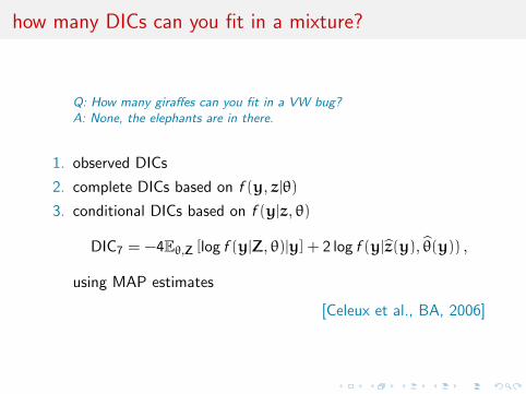
Q: How many giraffes can you fit in a VW bug?A: None, the elephants are in there.
1. observed DICs
DIC1 = −4Eθ [log f (y|θ)|y] + 2 log f (y|Eθ [θ|y])
often a poor choice in case of unidentifiability
2. complete DICs based on f (y, z|θ)
3. conditional DICs based on f (y|z, θ)
[Celeux et al., BA, 2006]

how many DICs can you fit in a mixture?
Q: How many giraffes can you fit in a VW bug?A: None, the elephants are in there.
1. observed DICs
DIC2 = −4Eθ [log f (y|θ)|y] + 2 log f (y|θ(y)) .
which uses posterior mode instead
2. complete DICs based on f (y, z|θ)
3. conditional DICs based on f (y|z, θ)
[Celeux et al., BA, 2006]

how many DICs can you fit in a mixture?
Q: How many giraffes can you fit in a VW bug?A: None, the elephants are in there.
1. observed DICs
DIC3 = −4Eθ [log f (y|θ)|y] + 2 log f (y) ,
which instead relies on the MCMC density estimate
2. complete DICs based on f (y, z|θ)
3. conditional DICs based on f (y|z, θ)
[Celeux et al., BA, 2006]

how many DICs can you fit in a mixture?
Q: How many giraffes can you fit in a VW bug?A: None, the elephants are in there.
1. observed DICs
2. complete DICs based on f (y, z|θ)
DIC4 = EZ [DIC(y,Z)|y]
= −4Eθ,Z [log f (y,Z|θ)|y] + 2EZ [log f (y,Z|Eθ[θ|y,Z])|y] .
3. conditional DICs based on f (y|z, θ)
[Celeux et al., BA, 2006]

how many DICs can you fit in a mixture?
Q: How many giraffes can you fit in a VW bug?A: None, the elephants are in there.
1. observed DICs
2. complete DICs based on f (y, z|θ)
DIC5 = −4Eθ,Z [log f (y,Z|θ)|y] + 2 log f (y, z(y)|θ(y)) ,
using Z as an additional parameter
3. conditional DICs based on f (y|z, θ)
[Celeux et al., BA, 2006]

how many DICs can you fit in a mixture?
Q: How many giraffes can you fit in a VW bug?A: None, the elephants are in there.
1. observed DICs
2. complete DICs based on f (y, z|θ)
DIC6 = −4Eθ,Z [log f (y,Z|θ)|y]+2EZ[log f (y,Z|θ(y))|y, θ(y)] .
in analogy with EM, θ being an EM fixed point
3. conditional DICs based on f (y|z, θ)
[Celeux et al., BA, 2006]
how many DICs can you fit in a mixture?
Q: How many giraffes can you fit in a VW bug?A: None, the elephants are in there.
1. observed DICs
2. complete DICs based on f (y, z|θ)
3. conditional DICs based on f (y|z, θ)
DIC7 = −4Eθ,Z [log f (y|Z, θ)|y] + 2 log f (y|z(y), θ(y)) ,
using MAP estimates
[Celeux et al., BA, 2006]

how many DICs can you fit in a mixture?
Q: How many giraffes can you fit in a VW bug?A: None, the elephants are in there.
1. observed DICs
2. complete DICs based on f (y, z|θ)
3. conditional DICs based on f (y|z, θ)
DIC8 = −4Eθ,Z [log f (y|Z, θ)|y]+2EZ[log f (y|Z, θ(y,Z))|y
],
conditioning first on Z and then integrating over Zconditional on y
[Celeux et al., BA, 2006]

Galactic DICs
Example of the galaxy mixture dataset
DIC2 DIC3 DIC4 DIC5 DIC6 DIC7 DIC8K (pD2) (pD3) (pD4) (pD5) (pD6) (pD7) (pD8)2 453 451 502 705 501 417 410
(5.56) (3.66) (5.50) (207.88) (4.48) (11.07) (4.09)3 440 436 461 622 471 378 372
(9.23) (4.94) (6.40) (167.28) (15.80) (13.59) (7.43)4 446 439 473 649 482 388 382
(11.58) (5.41) (7.52) (183.48) (16.51) (17.47) (11.37)5 447 442 485 658 511 395 390
(10.80) (5.48) (7.58) (180.73) (33.29) (20.00) (15.15)6 449 444 494 676 532 407 398
(11.26) (5.49) (8.49) (191.10) (46.83) (28.23) (19.34)7 460 446 508 700 571 425 409
(19.26) (5.83) (8.93) (200.35) (71.26) (40.51) (24.57)

questions
I what is the behaviour of DIC under model mispecification?
I is there an absolute scale to the DIC values, i.e. when is adifference in DICs significant?
I how can DIC handle small n’s versus p’s?
I should pD be defined as var(D |y)/2 [Gelman’s suggestion]?
I is WAIC (Gelman and Vehtari, 2013) making a difference forbeing based on expected posterior predictive?
In an era of complex models, is DIC applicable?[Robert, 2013]
Testing under incomplete information
Significance tests: one new parameter
Noninformative solutions
Jeffreys-Lindley paradox
Deviance (information criterion)
Testing under incomplete information
Testing via mixtures
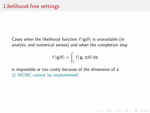
Likelihood-free settings
Cases when the likelihood function f (y|θ) is unavailable (inanalytic and numerical senses) and when the completion step
f (y|θ) =
∫Z
f (y, z|θ) dz
is impossible or too costly because of the dimension of zc© MCMC cannot be implemented!

The ABC method
Bayesian setting: target is π(θ)f (x |θ)When likelihood f (x |θ) not in closed form, likelihood-free rejectiontechnique:
ABC algorithm
For an observation y ∼ f (y|θ), under the prior π(θ), keep jointlysimulating
θ′ ∼ π(θ) , z ∼ f (z|θ′) ,
until the auxiliary variable z is equal to the observed value, z = y.
[Tavare et al., 1997]
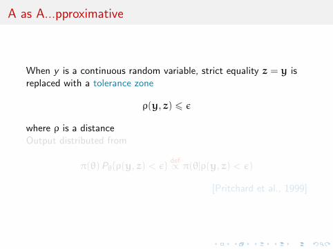
A as A...pproximative
When y is a continuous random variable, strict equality z = y isreplaced with a tolerance zone
ρ(y, z) 6 ε
where ρ is a distanceOutput distributed from
π(θ)Pθ{ρ(y, z) < ε}def∝ π(θ|ρ(y, z) < ε)
[Pritchard et al., 1999]

A as A...pproximative
When y is a continuous random variable, strict equality z = y isreplaced with a tolerance zone
ρ(y, z) 6 ε
where ρ is a distanceOutput distributed from
π(θ)Pθ{ρ(y, z) < ε}def∝ π(θ|ρ(y, z) < ε)
[Pritchard et al., 1999]

ABC algorithm
In most implementations, further degree of A...pproximation:
Algorithm 1 Likelihood-free rejection sampler
for i = 1 to N dorepeat
generate θ ′ from the prior distribution π(·)generate z from the likelihood f (·|θ ′)
until ρ{η(z),η(y)} 6 εset θi = θ
′
end for
where η(y) defines a (not necessarily sufficient) statistic
Which summary η(·)?
Fundamental difficulty of the choice of the summary statistic whenthere is no non-trivial sufficient statistics
I Loss of statistical information balanced against gain in dataroughening
I Approximation error and information loss remain unknown
I Choice of statistics induces choice of distance functiontowards standardisation
I may be imposed for external/practical reasons (e.g., LDA)
I may gather several non-B point estimates
I can learn about efficient combination
[Estoup et al., 2012, Genetics]

Generic ABC for model choice
Algorithm 2 Likelihood-free model choice sampler (ABC-MC)
for t = 1 to T dorepeat
Generate m from the prior π(M = m)Generate θm from the prior πm(θm)Generate z from the model fm(z|θm)
until ρ{η(z),η(y)} < εSet m(t) = m and θ(t) = θm
end for
[Grelaud et al., 2009]
ABC estimates
Posterior probability π(M = m|y) approximated by the frequencyof acceptances from model m
1
T
T∑t=1
Im(t)=m .
Issues with implementation:
I should tolerances ε be the same for all models?
I should summary statistics vary across models (incl. theirdimension)?
I should the distance measure ρ vary as well?

ABC estimates
Posterior probability π(M = m|y) approximated by the frequencyof acceptances from model m
1
T
T∑t=1
Im(t)=m .
Extension to a weighted polychotomous logistic regression estimateof π(M = m|y), with non-parametric kernel weights
[Cornuet et al., DIYABC, 2009]

ABCµ
Idea Infer about the error as well as about the parameter:Use of a joint density
f (θ, ε|y) ∝ ξ(ε|y, θ)× πθ(θ)× πε(ε)
where y is the data, and ξ(ε|y, θ) is the prior predictive density ofρ(η(z),η(y)) given θ and y when z ∼ f (z|θ)Warning! Replacement of ξ(ε|y, θ) with a non-parametric kernelapproximation.
[Ratmann, Andrieu, Wiuf and Richardson, 2009, PNAS]

ABCµ details
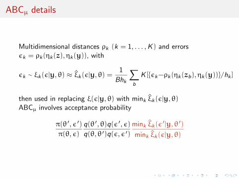
Multidimensional distances ρk (k = 1, . . . , K ) and errorsεk = ρk(ηk(z),ηk(y)), with
εk ∼ ξk(ε|y, θ) ≈ ξk(ε|y, θ) =1
Bhk
∑b
K [{εk−ρk(ηk(zb),ηk(y))}/hk ]
then used in replacing ξ(ε|y, θ) with mink ξk(ε|y, θ)ABCµ involves acceptance probability
π(θ ′, ε ′)
π(θ, ε)
q(θ ′, θ)q(ε ′, ε)
q(θ, θ ′)q(ε, ε ′)
mink ξk(ε′|y, θ ′)
mink ξk(ε|y, θ)
ABCµ details
Multidimensional distances ρk (k = 1, . . . , K ) and errorsεk = ρk(ηk(z),ηk(y)), with
εk ∼ ξk(ε|y, θ) ≈ ξk(ε|y, θ) =1
Bhk
∑b
K [{εk−ρk(ηk(zb),ηk(y))}/hk ]
then used in replacing ξ(ε|y, θ) with mink ξk(ε|y, θ)ABCµ involves acceptance probability
π(θ ′, ε ′)
π(θ, ε)
q(θ ′, θ)q(ε ′, ε)
q(θ, θ ′)q(ε, ε ′)
mink ξk(ε′|y, θ ′)
mink ξk(ε|y, θ)

ABCµ multiple errors
[ c© Ratmann et al., PNAS, 2009]

ABCµ for model choice
[ c© Ratmann et al., PNAS, 2009]
Questions about ABCµ [and model choice]
For each model under comparison, marginal posterior on ε used toassess the fit of the model (HPD includes 0 or not).
I Is the data informative about ε? [Identifiability]
I How much does the prior π(ε) impact the comparison?
I How is using both ξ(ε|x0, θ) and πε(ε) compatible with astandard probability model?
I Where is the penalisation for complexity in the modelcomparison?
[X, Mengersen & Chen, 2010, PNAS]

Formalised framework
Central question to the validation of ABC for model choice:
When is a Bayes factor based on an insufficient statistic T(y)consistent?
Note: c© drawn on T(y) through BT12(y) necessarily differs from
c© drawn on y through B12(y)

Formalised framework
Central question to the validation of ABC for model choice:
When is a Bayes factor based on an insufficient statistic T(y)consistent?
Note: c© drawn on T(y) through BT12(y) necessarily differs from
c© drawn on y through B12(y)

A benchmark if toy example
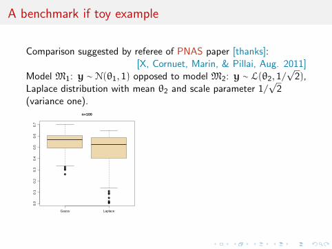
Comparison suggested by referee of PNAS paper [thanks]:[X, Cornuet, Marin, & Pillai, Aug. 2011]
Model M1: y ∼ N(θ1, 1) opposed to model M2: y ∼ L(θ2, 1/√
2),Laplace distribution with mean θ2 and scale parameter 1/
√2
(variance one).

A benchmark if toy example
Comparison suggested by referee of PNAS paper [thanks]:[X, Cornuet, Marin, & Pillai, Aug. 2011]
Model M1: y ∼ N(θ1, 1) opposed to model M2: y ∼ L(θ2, 1/√
2),Laplace distribution with mean θ2 and scale parameter 1/
√2
(variance one).Four possible statistics
1. sample mean y (sufficient for M1 if not M2);
2. sample median med(y) (insufficient);
3. sample variance var(y) (ancillary);
4. median absolute deviation mad(y) = med(y− med(y));

A benchmark if toy example
Comparison suggested by referee of PNAS paper [thanks]:[X, Cornuet, Marin, & Pillai, Aug. 2011]
Model M1: y ∼ N(θ1, 1) opposed to model M2: y ∼ L(θ2, 1/√
2),Laplace distribution with mean θ2 and scale parameter 1/
√2
(variance one).
0.1 0.2 0.3 0.4 0.5 0.6 0.7
01
23
45
6
posterior probability
Den
sity
A benchmark if toy example
Comparison suggested by referee of PNAS paper [thanks]:[X, Cornuet, Marin, & Pillai, Aug. 2011]
Model M1: y ∼ N(θ1, 1) opposed to model M2: y ∼ L(θ2, 1/√
2),Laplace distribution with mean θ2 and scale parameter 1/
√2
(variance one).
●
●
●
●
●
●
●●
●
●
●
Gauss Laplace
0.0
0.1
0.2
0.3
0.4
0.5
0.6
0.7
n=100

A benchmark if toy example
Comparison suggested by referee of PNAS paper [thanks]:[X, Cornuet, Marin, & Pillai, Aug. 2011]
Model M1: y ∼ N(θ1, 1) opposed to model M2: y ∼ L(θ2, 1/√
2),Laplace distribution with mean θ2 and scale parameter 1/
√2
(variance one).
0.1 0.2 0.3 0.4 0.5 0.6 0.7
01
23
45
6
posterior probability
Den
sity
0.0 0.2 0.4 0.6 0.8 1.0
01
23
probability
Den
sity

A benchmark if toy example
Comparison suggested by referee of PNAS paper [thanks]:[X, Cornuet, Marin, & Pillai, Aug. 2011]
Model M1: y ∼ N(θ1, 1) opposed to model M2: y ∼ L(θ2, 1/√
2),Laplace distribution with mean θ2 and scale parameter 1/
√2
(variance one).
●
●
●
●
●
●
●●
●
●
●
Gauss Laplace
0.0
0.1
0.2
0.3
0.4
0.5
0.6
0.7
n=100
●●
●
●
●
●
●
●
●
●
●
●
●
●
●
●●
●
Gauss Laplace
0.0
0.2
0.4
0.6
0.8
1.0
n=100

Consistency theorem
If Pn belongs to one of the two models and if µ0 = E[T] cannot beattained by the other one :
0 = min (inf{|µ0 − µi (θi )|; θi ∈ Θi }, i = 1, 2)
< max (inf{|µ0 − µi (θi )|; θi ∈ Θi }, i = 1, 2) ,
then the Bayes factor BT12 is consistent

Conclusion
Model selection feasible with ABC:
I Choice of summary statistics is paramount
I At best, ABC output → π(. | η(y)) which concentratesaround µ0
I For estimation : {θ;µ(θ) = µ0} = θ0
I For testing {µ1(θ1), θ1 ∈ Θ1} ∩ {µ2(θ2), θ2 ∈ Θ2} = ∅
[Marin et al., 2013]

Conclusion
Model selection feasible with ABC:
I Choice of summary statistics is paramount
I At best, ABC output → π(. | η(y)) which concentratesaround µ0
I For estimation : {θ;µ(θ) = µ0} = θ0
I For testing {µ1(θ1), θ1 ∈ Θ1} ∩ {µ2(θ2), θ2 ∈ Θ2} = ∅
[Marin et al., 2013]
Changing the testing perspective
Significance tests: one new parameter
Noninformative solutions
Jeffreys-Lindley paradox
Deviance (information criterion)
Testing under incomplete information
Testing via mixtures

Testing issues
Hypothesis testing
I central problem of statistical inference
I dramatically differentiating feature between classical andBayesian paradigms
I wide open to controversy and divergent opinions, includ.within the Bayesian community
I non-informative Bayesian testing case mostly unresolved,witness the Jeffreys–Lindley paradox
[Berger (2003), Mayo & Cox (2006), Gelman (2008)]

Testing hypotheses
I Bayesian model selection as comparison of k potentialstatistical models towards the selection of model that fits thedata “best”
I mostly accepted perspective: it does not primarily seek toidentify which model is “true”, but compares fits
I tools like Bayes factor naturally include a penalisationaddressing model complexity, mimicked by Bayes Information(BIC) and Deviance Information (DIC) criteria
I posterior predictive tools successfully advocated in Gelman etal. (2013) even though they involve double use of data
Some difficulties
I tension between using (i) posterior probabilities justified by abinary loss function but depending on unnatural prior weights,and (ii) Bayes factors that eliminate this dependence butescape direct connection with posterior distribution, unlessprior weights are integrated within the loss
I subsequent and delicate interpretation (or calibration) of thestrength of the Bayes factor towards supporting a givenhypothesis or model, because it is not a Bayesian decision rule
I similar difficulty with posterior probabilities, with tendency tointerpret them as p-values (rather than the opposite!) whenthey only report through a marginal likelihood ratio therespective strengths of fitting the data to both models
Some further difficulties
I long-lasting impact of the prior modeling, meaning the choiceof the prior distributions on the parameter spaces of bothmodels under comparison, despite overall consistency proof forBayes factor
I discontinuity in use of improper priors since they are notjustified in most testing situations, leading to many alternativeif ad hoc solutions, where data is either used twice or split inartificial ways
I binary (accept vs. reject) outcome more suited for immediatedecision (if any) than for model evaluation, in connection withrudimentary loss function

Some additional difficulties
I related impossibility to ascertain simultaneous misfit or todetect presence of outliers
I no assessment of uncertainty associated with decision itself
I difficult computation of marginal likelihoods in most settingswith further controversies about which algorithm to adopt
I strong dependence of posterior probabilities on conditioningstatistics, which in turn undermines their validity for modelassessment, as exhibited in ABC model choice
I temptation to create pseudo-frequentist equivalents such asq-values with even less Bayesian justifications

Paradigm shift
New proposal for a paradigm shift in the Bayesian processing ofhypothesis testing and of model selection
I convergent and naturally interpretable solution
I more extended use of improper priors
Simple representation of the testing problem as atwo-component mixture estimation problem where theweights are formally equal to 0 or 1

Paradigm shift
Simple representation of the testing problem as atwo-component mixture estimation problem where theweights are formally equal to 0 or 1
I Approach inspired from consistency result of Rousseau andMengersen (2011) on estimated overfitting mixtures
I Mixture representation not directly equivalent to the use of aposterior probability
I Potential of a better approach to testing, while not expandingnumber of parameters
I Calibration of the posterior distribution of the weight of amodel, while moving from the artificial notion of the posteriorprobability of a model

Encompassing mixture model
Idea: Given two statistical models,
M1 : x ∼ f1(x |θ1) , θ1 ∈ Θ1 and M2 : x ∼ f2(x |θ2) , θ2 ∈ Θ2 ,
embed both within an encompassing mixture
Mα : x ∼ αf1(x |θ1) + (1 − α)f2(x |θ2) , 0 6 α 6 1 (1)
Note: Both models correspond to special cases of (1), one forα = 1 and one for α = 0Draw inference on mixture representation (1), as if eachobservation was individually and independently produced by themixture model

Inferential motivations
Sounds like an approximation to the real model, but severaldefinitive advantages to this paradigm shift:
I Bayes estimate of the weight α replaces posterior probabilityof model M1, equally convergent indicator of which model is“true”, while avoiding artificial prior probabilities on modelindices, ω1 and ω2
I interpretation of estimator of α at least as natural as handlingthe posterior probability, while avoiding zero-one loss setting
I α and its posterior distribution provide measure of proximityto the models, while being interpretable as data propensity tostand within one model
I further allows for alternative perspectives on testing andmodel choice, like predictive tools, cross-validation, andinformation indices like WAIC
Computational motivations
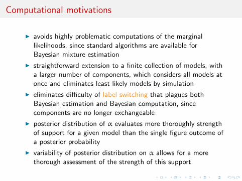
I avoids highly problematic computations of the marginallikelihoods, since standard algorithms are available forBayesian mixture estimation
I straightforward extension to a finite collection of models, witha larger number of components, which considers all models atonce and eliminates least likely models by simulation
I eliminates difficulty of label switching that plagues bothBayesian estimation and Bayesian computation, sincecomponents are no longer exchangeable
I posterior distribution of α evaluates more thoroughly strengthof support for a given model than the single figure outcome ofa posterior probability
I variability of posterior distribution on α allows for a morethorough assessment of the strength of this support

Noninformative motivations
I additional feature missing from traditional Bayesian answers:a mixture model acknowledges possibility that, for a finitedataset, both models or none could be acceptable
I standard (proper and informative) prior modeling can bereproduced in this setting, but non-informative (improper)priors also are manageable therein, provided both models firstreparameterised towards shared parameters, e.g. location andscale parameters
I in special case when all parameters are common
Mα : x ∼ αf1(x |θ) + (1 − α)f2(x |θ) , 0 6 α 6 1
if θ is a location parameter, a flat prior π(θ) ∝ 1 is available

Weakly informative motivations
I using the same parameters or some identical parameters onboth components highlights that opposition between the twocomponents is not an issue of enjoying different parameters
I those common parameters are nuisance parameters, to beintegrated out
I prior model weights ωi rarely discussed in classical Bayesianapproach, even though linear impact on posterior probabilities.Here, prior modeling only involves selecting a prior on α, e.g.,α ∼ B(a0, a0)
I while a0 impacts posterior on α, it always leads to massaccumulation near 1 or 0, i.e. favours most likely model
I sensitivity analysis straightforward to carry
I approach easily calibrated by parametric boostrap providingreference posterior of α under each model
I natural Metropolis–Hastings alternative

Poisson/Geometric
I choice betwen Poisson P(λ) and Geometric Geo(p)distribution
I mixture with common parameter λ
Mα : αP(λ) + (1 − α)Geo(1/1+λ)
Allows for Jeffreys prior since resulting posterior is proper
I independent Metropolis–within–Gibbs with proposaldistribution on λ equal to Poisson posterior (with acceptancerate larger than 75%)

Beta prior
When α ∼ Be(a0, a0) prior, full conditional posterior
α ∼ Be(n1(ζ) + a0, n2(ζ) + a0)
Exact Bayes factor opposing Poisson and Geometric
B12 = nnxn
n∏i=1
xi ! Γ
(n + 2 +
n∑i=1
xi
)/Γ(n + 2)
although undefined from a purely mathematical viewpoint
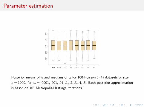
Parameter estimation
1e-04 0.001 0.01 0.1 0.2 0.3 0.4 0.5
3.90
3.95
4.00
4.05
4.10
Posterior means of λ and medians of α for 100 Poisson P(4) datasets of size
n = 1000, for a0 = .0001, .001, .01, .1, .2, .3, .4, .5. Each posterior approximation
is based on 104 Metropolis-Hastings iterations.

Parameter estimation
1e-04 0.001 0.01 0.1 0.2 0.3 0.4 0.5
0.990
0.992
0.994
0.996
0.998
1.000
Posterior means of λ and medians of α for 100 Poisson P(4) datasets of size
n = 1000, for a0 = .0001, .001, .01, .1, .2, .3, .4, .5. Each posterior approximation
is based on 104 Metropolis-Hastings iterations.
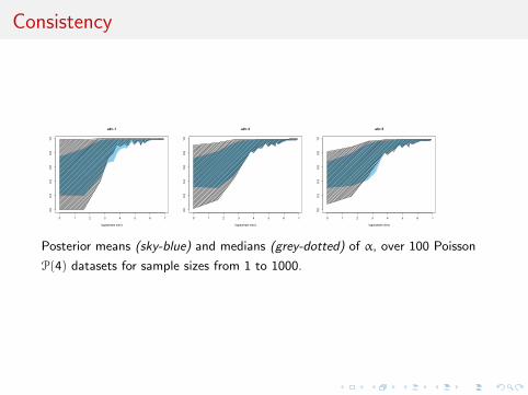
Consistency
0 1 2 3 4 5 6 7
0.0
0.2
0.4
0.6
0.8
1.0
a0=.1
log(sample size)
0 1 2 3 4 5 6 7
0.0
0.2
0.4
0.6
0.8
1.0
a0=.3
log(sample size)
0 1 2 3 4 5 6 7
0.0
0.2
0.4
0.6
0.8
1.0
a0=.5
log(sample size)
Posterior means (sky-blue) and medians (grey-dotted) of α, over 100 Poisson
P(4) datasets for sample sizes from 1 to 1000.

Behaviour of Bayes factor
0 1 2 3 4 5 6 7
0.0
0.2
0.4
0.6
0.8
1.0
log(sample size)
0 1 2 3 4 5 6 7
0.0
0.2
0.4
0.6
0.8
1.0
log(sample size)
0 1 2 3 4 5 6 7
0.0
0.2
0.4
0.6
0.8
1.0
log(sample size)
Comparison between P(M1|x) (red dotted area) and posterior medians of α
(grey zone) for 100 Poisson P(4) datasets with sample sizes n between 1 and
1000, for a0 = .001, .1, .5

Normal-normal comparison
I comparison of a normal N(θ1, 1) with a normal N(θ2, 2)distribution
I mixture with identical location parameter θαN(θ, 1) + (1 − α)N(θ, 2)
I Jeffreys prior π(θ) = 1 can be used, since posterior is proper
I Reference (improper) Bayes factor
B12 = 2n−1/2
/exp 1/4
n∑i=1
(xi − x)2 ,

Consistency
0.1 0.2 0.3 0.4 0.5 p(M1|x)
0.0
0.2
0.4
0.6
0.8
1.0
n=15
0.0
0.2
0.4
0.6
0.8
1.0
0.1 0.2 0.3 0.4 0.5 p(M1|x)
0.65
0.70
0.75
0.80
0.85
0.90
0.95
1.00
n=50
0.65
0.70
0.75
0.80
0.85
0.90
0.95
1.00
0.1 0.2 0.3 0.4 0.5 p(M1|x)
0.75
0.80
0.85
0.90
0.95
1.00
n=100
0.75
0.80
0.85
0.90
0.95
1.00
0.1 0.2 0.3 0.4 0.5 p(M1|x)
0.93
0.94
0.95
0.96
0.97
0.98
0.99
1.00
n=500
0.93
0.94
0.95
0.96
0.97
0.98
0.99
1.00
Posterior means (wheat) and medians of α (dark wheat), compared with
posterior probabilities of M0 (gray) for a N(0, 1) sample, derived from 100
datasets for sample sizes equal to 15, 50, 100, 500. Each posterior
approximation is based on 104 MCMC iterations.

Comparison with posterior probability
0 100 200 300 400 500
-50
-40
-30
-20
-10
0
a0=.1
sample size
0 100 200 300 400 500
-50
-40
-30
-20
-10
0
a0=.3
sample size
0 100 200 300 400 500
-50
-40
-30
-20
-10
0
a0=.4
sample size
0 100 200 300 400 500
-50
-40
-30
-20
-10
0
a0=.5
sample size
Plots of ranges of log(n) log(1−E[α|x ]) (gray color) and log(1− p(M1|x)) (red
dotted) over 100 N(0, 1) samples as sample size n grows from 1 to 500. and α
is the weight of N(0, 1) in the mixture model. The shaded areas indicate the
range of the estimations and each plot is based on a Beta prior with
a0 = .1, .2, .3, .4, .5, 1 and each posterior approximation is based on 104
iterations.

Comments
I convergence to one boundary value as sample size n grows
I impact of hyperarameter a0 slowly vanishes as n increases, butpresent for moderate sample sizes
I when simulated sample is neither from N(θ1, 1) nor fromN(θ2, 2), behaviour of posterior varies, depending on whichdistribution is closest

Logit or Probit?
I binary dataset, R dataset about diabetes in 200 Pima Indianwomen with body mass index as explanatory variable
I comparison of logit and probit fits could be suitable. We arethus comparing both fits via our method
M1 : yi | xi , θ1 ∼ B(1, pi ) where pi =
exp(xiθ1)
1 + exp(xiθ1)
M2 : yi | xi , θ2 ∼ B(1, qi ) where qi = Φ(xiθ2)
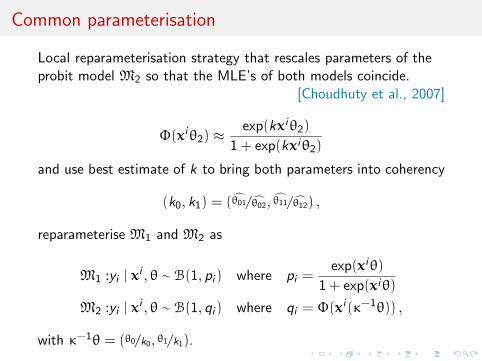
Common parameterisation
Local reparameterisation strategy that rescales parameters of theprobit model M2 so that the MLE’s of both models coincide.
[Choudhuty et al., 2007]
Φ(xiθ2) ≈exp(kxiθ2)
1 + exp(kxiθ2)
and use best estimate of k to bring both parameters into coherency
(k0, k1) = (θ01/θ02, θ11/θ12) ,
reparameterise M1 and M2 as
M1 :yi | xi , θ ∼ B(1, pi ) where pi =
exp(xiθ)
1 + exp(xiθ)
M2 :yi | xi , θ ∼ B(1, qi ) where qi = Φ(xi (κ−1θ)) ,
with κ−1θ = (θ0/k0, θ1/k1).

Prior modelling
Under default g -prior
θ ∼ N2(0, n(XTX )−1)
full conditional posterior distributions given allocations
π(θ | y, X , ζ) ∝exp{∑
i Iζi=1yixiθ}∏
i ;ζi=1[1 + exp(xiθ)]exp{−θT (XTX )θ
/2n}
×∏i ;ζi=2
Φ(xi (κ−1θ))yi (1 −Φ(xi (κ−1θ)))(1−yi)
hence posterior distribution clearly defined
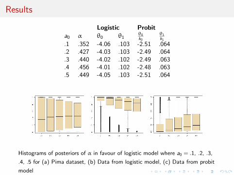
Results
Logistic Probita0 α θ0 θ1
θ0
k0θ1
k1.1 .352 -4.06 .103 -2.51 .064.2 .427 -4.03 .103 -2.49 .064.3 .440 -4.02 .102 -2.49 .063.4 .456 -4.01 .102 -2.48 .063.5 .449 -4.05 .103 -2.51 .064
Histograms of posteriors of α in favour of logistic model where a0 = .1, .2, .3,
.4, .5 for (a) Pima dataset, (b) Data from logistic model, (c) Data from probit
model
Survival analysis
Testing hypothesis that data comes from a
1. log-Normal(φ, κ2),
2. Weibull(α, λ), or
3. log-Logistic(γ, δ)
distribution
Corresponding mixture given by the density
α1 exp{−(log x − φ)2/2κ2}/√
2πxκ+
α2α
λexp{−(x/λ)α}((x/λ)α−1+
α3(δ/γ)(x/γ)δ−1/(1 + (x/γ)δ)2
where α1 + α2 + α3 = 1

Survival analysis
Testing hypothesis that data comes from a
1. log-Normal(φ, κ2),
2. Weibull(α, λ), or
3. log-Logistic(γ, δ)
distribution
Corresponding mixture given by the density
α1 exp{−(log x − φ)2/2κ2}/√
2πxκ+
α2α
λexp{−(x/λ)α}((x/λ)α−1+
α3(δ/γ)(x/γ)δ−1/(1 + (x/γ)δ)2
where α1 + α2 + α3 = 1

Reparameterisation
Looking for common parameter(s):
φ = µ+ γβ = ξ
σ2 = π2β2/6 = ζ2π2/3
where γ ≈ 0.5772 is Euler-Mascheroni constant.
Allows for a noninformative prior on the common location scaleparameter,
π(φ,σ2) = 1/σ2
Reparameterisation
Looking for common parameter(s):
φ = µ+ γβ = ξ
σ2 = π2β2/6 = ζ2π2/3
where γ ≈ 0.5772 is Euler-Mascheroni constant.
Allows for a noninformative prior on the common location scaleparameter,
π(φ,σ2) = 1/σ2

Recovery
.01 0.1 1.0 10.0
0.86
0.88
0.90
0.92
0.94
0.96
0.98
1.00
.01 0.1 1.0 10.00.00
0.02
0.04
0.06
0.08
Boxplots of the posterior distributions of the Normal weight α1 under the two
scenarii: truth = Normal (left panel), truth = Gumbel (right panel), a0=0.01,
0.1, 1.0, 10.0 (from left to right in each panel) and n = 10, 000 simulated
observations.

Asymptotic consistency
Posterior consistency holds for mixture testing procedure [underminor conditions]
Two different cases
I the two models, M1 and M2, are well separated
I model M1 is a submodel of M2.
Asymptotic consistency
Posterior consistency holds for mixture testing procedure [underminor conditions]
Two different cases
I the two models, M1 and M2, are well separated
I model M1 is a submodel of M2.

Posterior concentration rate
Let π be the prior and xn = (x1, · · · , xn) a sample with truedensity f ∗
propositionAssume that, for all c > 0, there exist Θn ⊂ Θ1 ×Θ2 and B > 0 such that
π [Θcn] 6 n−c , Θn ⊂ {‖θ1‖+ ‖θ2‖ 6 nB }
and that there exist H > 0 and L, δ > 0 such that, for j = 1, 2,
supθ,θ′∈Θn
‖fj,θj − fj,θ′j‖1 6 LnH‖θj − θ ′j ‖, θ = (θ1, θ2), θ
′= (θ
′1, θ′2) ,
∀‖θj − θ∗j ‖ 6 δ; KL(fj,θj , fj,θ∗j ) . ‖θj − θ∗j ‖ .
Then, when f ∗ = fθ∗,α∗ , with α∗ ∈ [0, 1], there exists M > 0 such that
π[(α, θ); ‖fθ,α − f ∗‖1 > M
√log n/n|xn
]= op(1) .
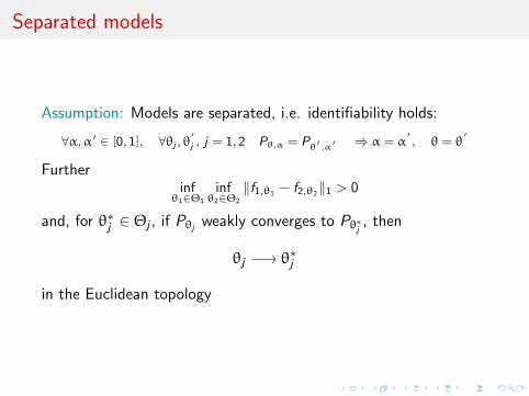
Separated models
Assumption: Models are separated, i.e. identifiability holds:
∀α,α ′ ∈ [0, 1], ∀θj , θ′j , j = 1, 2 Pθ,α = Pθ′ ,α′ ⇒ α = α
′, θ = θ
′
Furtherinfθ1∈Θ1
infθ2∈Θ2
‖f1,θ1− f2,θ2
‖1 > 0
and, for θ∗j ∈ Θj , if Pθj weakly converges to Pθ∗j , then
θj −→ θ∗j
in the Euclidean topology

Separated models
Assumption: Models are separated, i.e. identifiability holds:
∀α,α ′ ∈ [0, 1], ∀θj , θ′j , j = 1, 2 Pθ,α = Pθ′ ,α′ ⇒ α = α
′, θ = θ
′
theorem
Under above assumptions, then for all ε > 0,
π [|α− α∗| > ε|xn] = op(1)

Separated models
Assumption: Models are separated, i.e. identifiability holds:
∀α,α ′ ∈ [0, 1], ∀θj , θ′j , j = 1, 2 Pθ,α = Pθ′ ,α′ ⇒ α = α
′, θ = θ
′
theorem
If
I θj → fj ,θj is C2 around θ∗j , j = 1, 2,
I f1,θ∗1− f2,θ∗2
,∇f1,θ∗1,∇f2,θ∗2
are linearly independent in y and
I there exists δ > 0 such that
∇f1,θ∗1 , ∇f2,θ∗2 , sup|θ1−θ
∗1 |<δ
|D2f1,θ1 |, sup|θ2−θ
∗2 |<δ
|D2f2,θ2 | ∈ L1
thenπ[|α− α∗| > M
√log n/n
∣∣xn] = op(1).

Separated models
Assumption: Models are separated, i.e. identifiability holds:
∀α,α ′ ∈ [0, 1], ∀θj , θ′j , j = 1, 2 Pθ,α = Pθ′ ,α′ ⇒ α = α
′, θ = θ
′
theorem allows for interpretation of α under the posterior: If dataxn is generated from model M1 then posterior on α concentratesaround α = 1
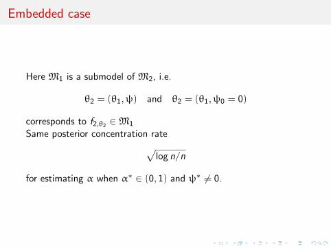
Embedded case
Here M1 is a submodel of M2, i.e.
θ2 = (θ1,ψ) and θ2 = (θ1,ψ0 = 0)
corresponds to f2,θ2 ∈M1
Same posterior concentration rate√log n/n
for estimating α when α∗ ∈ (0, 1) and ψ∗ 6= 0.
Null case
I Case where ψ∗ = 0, i.e., f ∗ is in model M1
I Two possible paths to approximate f ∗: either α goes to 1(path 1) or ψ goes to 0 (path 2)
I New identifiability condition: Pθ,α = P∗ only if
α = 1, θ1 = θ∗1 , θ2 = (θ∗1 ,ψ) or α 6 1, θ1 = θ
∗1 , θ2 = (θ∗1 , 0)
Priorπ(α, θ) = πα(α)π1(θ1)πψ(ψ), θ2 = (θ1,ψ)
with common (prior on) θ1
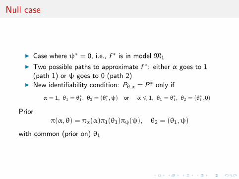
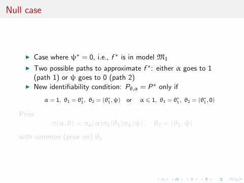

Assumptions
[B1] Regularity : Assume that θ1 → f1,θ1 and θ2 → f2,θ2 are 3times continuously differentiable and that
F ∗
(f 31,θ∗1
f 31,θ∗1
)< +∞, f1,θ∗1 = sup
|θ1−θ∗1 |<δ
f1,θ1 , f 1,θ∗1= inf
|θ1−θ∗1 |<δ
f1,θ1
F ∗
(sup|θ1−θ∗1 |<δ |∇f1,θ∗1 |
3
f 31,θ∗1
)< +∞, F ∗
(|∇f1,θ∗1 |
4
f 41,θ∗1
)< +∞,
F ∗
(sup|θ1−θ∗1 |<δ |D
2f1,θ∗1 |2
f 21,θ∗1
)< +∞, F ∗
(sup|θ1−θ∗1 |<δ |D
3f1,θ∗1 |
f 1,θ∗1
)< +∞

Assumptions
[B2] Integrability : There exists
S0 ⊂ S ∩ {|ψ| > δ0}
for some positive δ0 and satisfying Leb(S0) > 0, and such that forall ψ ∈ S0,
F ∗
(sup|θ1−θ∗1 |<δ f2,θ1,ψ
f 41,θ∗1
)< +∞, F ∗
(sup|θ1−θ∗1 |<δ f 3
2,θ1,ψ
f 31,θ1∗
)< +∞,
Assumptions
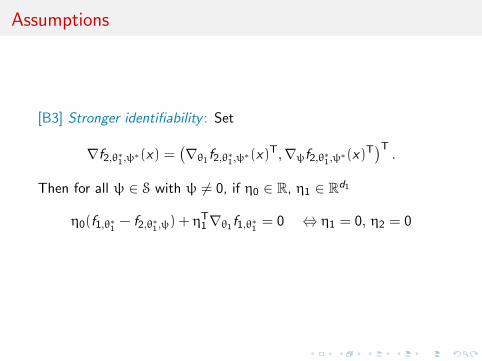
[B3] Stronger identifiability : Set
∇f2,θ∗1 ,ψ∗(x) =(∇θ1f2,θ∗1 ,ψ∗(x)
T,∇ψf2,θ∗1 ,ψ∗(x)T)T
.
Then for all ψ ∈ S with ψ 6= 0, if η0 ∈ R, η1 ∈ Rd1
η0(f1,θ∗1− f2,θ∗1 ,ψ) + η
T1∇θ1f1,θ∗1
= 0 ⇔ η1 = 0, η2 = 0

Consistency
theorem
Given the mixture fθ1,ψ,α = αf1,θ1 + (1 − α)f2,θ1,ψ and a samplexn = (x1, · · · , xn) issued from f1,θ∗1
, under assumptions B1 − B3,and an M > 0 such that
π[(α, θ); ‖fθ,α − f ∗‖1 > M
√log n/n|xn
]= op(1).
If α ∼ B(a1, a2), with a2 < d2, and if the prior πθ1,ψ is absolutelycontinuous with positive and continuous density at (θ∗1 , 0), then forMn −→∞π[|α− α∗| > Mn(log n)γ/
√n|xn
]= op(1), γ = max((d1 + a2)/(d2 − a2), 1)/2,


![[FRC 2015] Driver Station Tutorial](https://static.documents.pub/doc/80x56/563db9b8550346aa9a9f49ea/frc-2015-driver-station-tutorial.jpg)


![EL LXIC POPULAR VALENCIÀ EN LA LITERATURA DE …projectetraces.uab.cat/tracesbd/caplletra/2015/caplletra_a2015m10n... · poble honrat, el que treballa y riu [...], ham d’anar buscant](https://static.documents.pub/doc/80x56/5a78fd6f7f8b9adb5a8c4ab5/el-lxic-popular-valenci-en-la-literatura-de-honrat-el-que-treballa-y-riu-.jpg)
