Tutorial: Stochastic Modeling in Biology Applications of Discrete- Time Markov Chains Linda J. S. Allen Texas Tech University Lubbock, Texas U.S.A. NIMBioS Knoxville, Tennessee March 16-18, 2011 L. J. S. Allen Texas Tech University
Transcript
Tutorial: Stochastic Modeling in BiologyApplications of Discrete- Time Markov Chains
Linda J. S. AllenTexas Tech University
Lubbock, Texas U.S.A.
NIMBioSKnoxville, TennesseeMarch 16-18, 2011
L. J. S. Allen Texas Tech University
OUTLINE
Part I: Discrete-Time Markov Chains - DTMC
• Summary of Notation
• Applications:
(1) Proliferating Cells [Matlab program]
(2) Restricted Random Walk [Matlab program]
(3) Simple Birth and Death Process
(4) SIS Epidemic Process [Matlab program]
Part II: Discrete-Time Branching Processes
• Summary of Notation
• Applications:
(1) Cell Cycle
(2) Age-Structured Population
L. J. S. Allen Texas Tech University
References for these Notes
1. Allen, EJ 2007 Modeling with Ito Stochastic Differential Equations.Springer, Dordrecht, The Netherlands
2. Allen, LJS 2010 An Introduction to Stochastic Processes withApplications to Biology. 2nd Ed. CRC Press/Chapman & Hall,Boca Raton, Fl
3. Allen, LJS 2008 Chapter 3: An Introduction to StochasticEpidemic Models. Mathematical Epidemiology, Lecture Notesin Mathematics. Vol. 1945. pp. 81-130, F Brauer, P van denDriessche, and J Wu (Eds) Springer
4. Athreya, KB and P Ney 197. Branching Processes. Springer, Berlin
5. Caswell, H 2001 Matrix Population Models. 2nd Ed. Sinauer Assoc.Inc., Sunderland, MA
6. Karlin S and H Taylor 1975 A First Course in Stochastic Processes.2nd Ed. Acad. Press, NY
L. J. S. Allen Texas Tech University
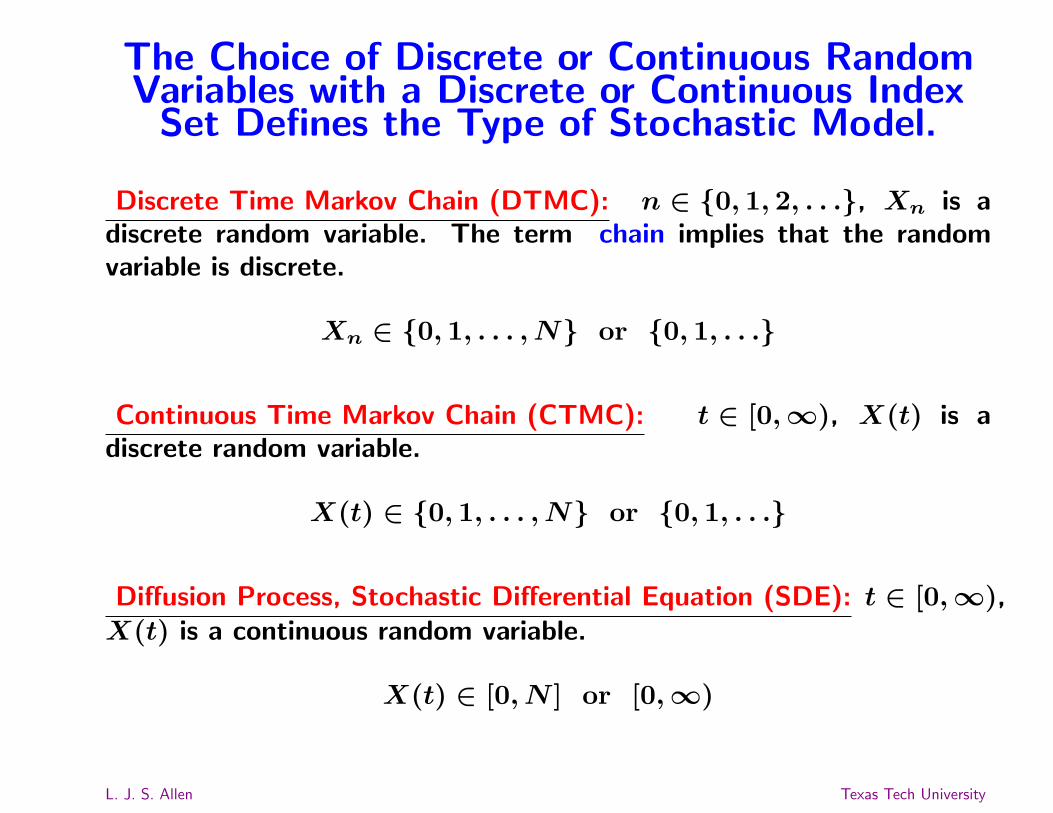
The Choice of Discrete or Continuous RandomVariables with a Discrete or Continuous Index
Set Defines the Type of Stochastic Model.
Discrete Time Markov Chain (DTMC): n ∈ {0, 1, 2, . . .}, Xn is adiscrete random variable. The term chain implies that the randomvariable is discrete.
Xn ∈ {0, 1, . . . , N} or {0, 1, . . .}
Continuous Time Markov Chain (CTMC): t ∈ [0,∞), X(t) is adiscrete random variable.
X(t) ∈ {0, 1, . . . , N} or {0, 1, . . .}
Diffusion Process, Stochastic Differential Equation (SDE): t ∈ [0,∞),X(t) is a continuous random variable.
X(t) ∈ [0, N ] or [0,∞)
L. J. S. Allen Texas Tech University
Part I:Discrete-Time Markov Chains
Notation and Terminology
Discrete random variable: Xn, n ∈ {0, 1, 2, . . .} with state space
{0, 1, 2, . . . , N} or {0, 1, 2, . . .}.
Markov property:
Prob{Xn = in|X0 = i0, . . . , Xn−1 = in−1}
= Prob{Xn = in|Xn−1 = in−1}.
Probability mass function of Xn: {pi(n)}∞i=0, where
pi(n) = Prob{Xn = i}.
L. J. S. Allen Texas Tech University
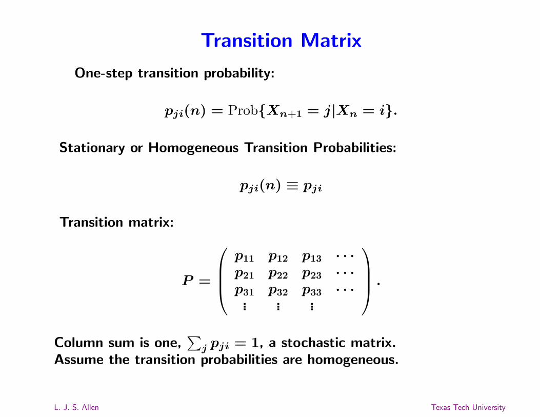
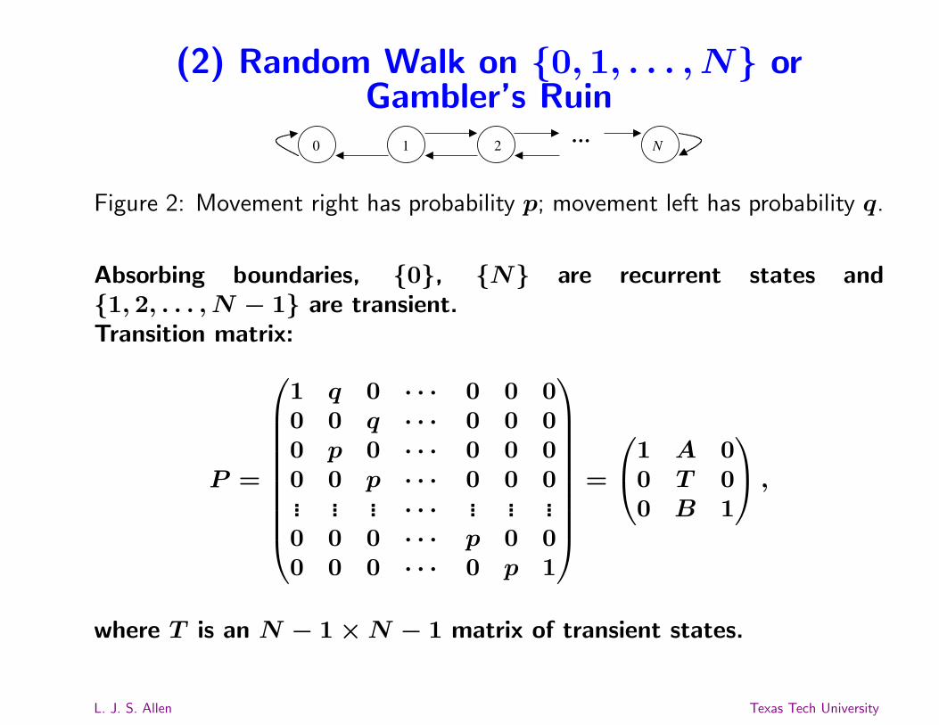
Transition Matrix
One-step transition probability:
pji(n) = Prob{Xn+1 = j|Xn = i}.
Stationary or Homogeneous Transition Probabilities:
Figure 1: Cell division results in two new vertices and three new sides per cell.
Proliferating epithelial cells in animal tissues have a polygonalshape with most cells being hexagonal (six-sided). An infinite MC isapproximated by a finite positive recurrent MC to show the highestprobability among all of the polygonal shapes is six-sided.
Gibson et al. 2006 Nature
L. J. S. Allen Texas Tech University
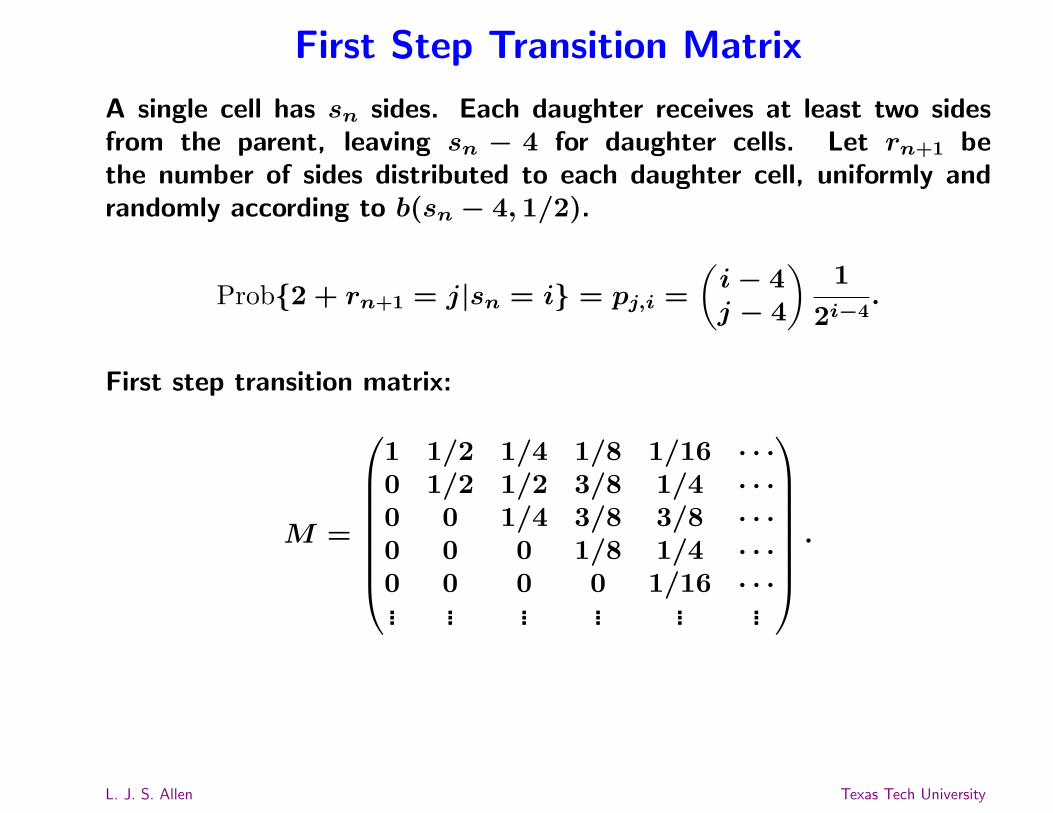
First Step Transition Matrix
A single cell has sn sides. Each daughter receives at least two sidesfrom the parent, leaving sn − 4 for daughter cells. Let rn+1 bethe number of sides distributed to each daughter cell, uniformly andrandomly according to b(sn − 4, 1/2).
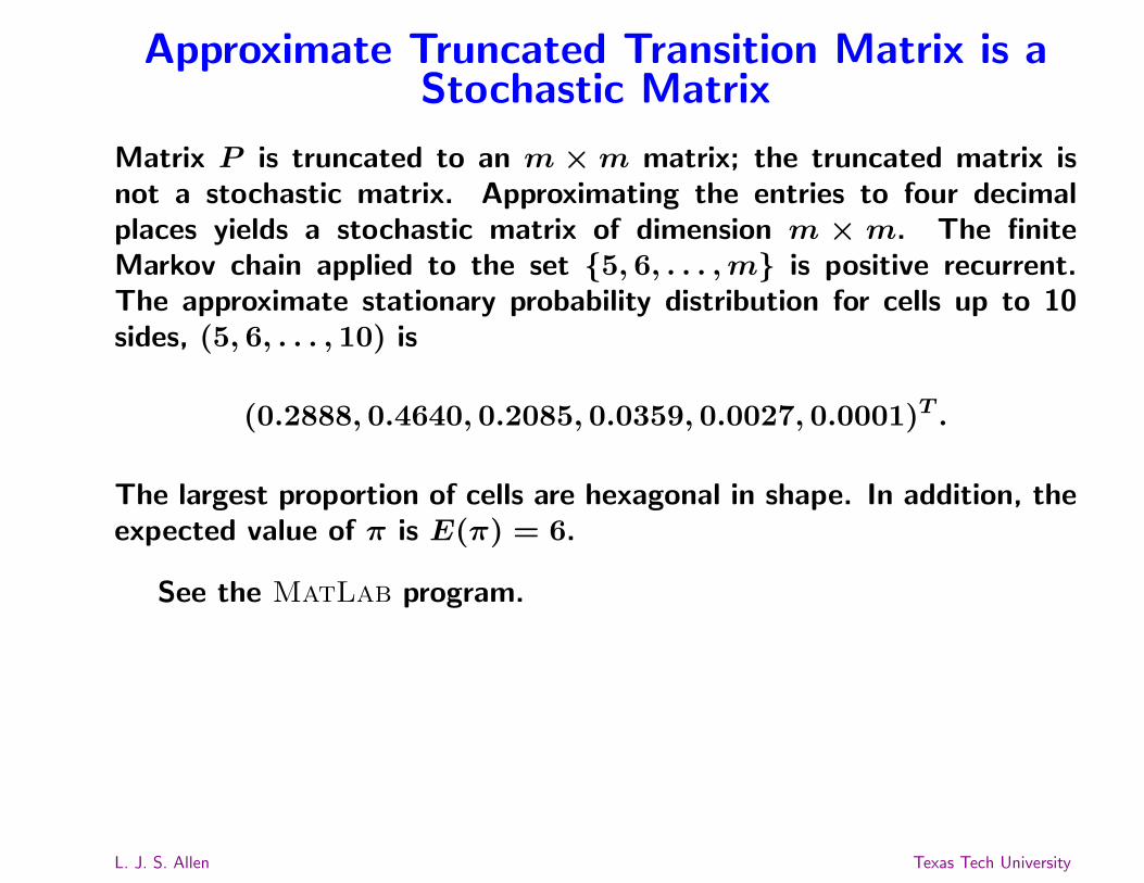
Approximate Truncated Transition Matrix is aStochastic Matrix
Matrix P is truncated to an m ×m matrix; the truncated matrix isnot a stochastic matrix. Approximating the entries to four decimalplaces yields a stochastic matrix of dimension m × m. The finiteMarkov chain applied to the set {5, 6, . . . ,m} is positive recurrent.The approximate stationary probability distribution for cells up to 10sides, (5, 6, . . . , 10) is
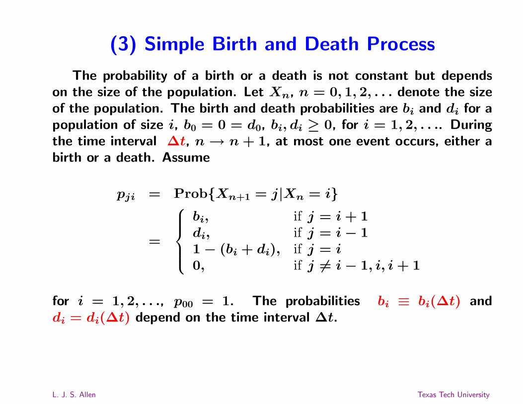
The probability of a birth or a death is not constant but dependson the size of the population. Let Xn, n = 0, 1, 2, . . . denote the sizeof the population. The birth and death probabilities are bi and di for apopulation of size i, b0 = 0 = d0, bi, di ≥ 0, for i = 1, 2, . . .. Duringthe time interval ∆t, n→ n+ 1, at most one event occurs, either abirth or a death. Assume
pji = Prob{Xn+1 = j|Xn = i}
=
bi, if j = i+ 1di, if j = i− 11− (bi + di), if j = i0, if j 6= i− 1, i, i+ 1
for i = 1, 2, . . ., p00 = 1. The probabilities bi ≡ bi(∆t) anddi = di(∆t) depend on the time interval ∆t.
L. J. S. Allen Texas Tech University
The Transition Matrix for a Birth and DeathProcess
The transition matrix P has the following form:1 d1 0 · · ·0 1− (b1 + d1) d2 · · ·0 b1 1− (b2 + d2) · · ·0 0 b2 · · ·... ... ... ...
=(
1 A0 T
).
During the time interval ∆t, either the population size increases byone, decreases by one, or stays the same size. This is a reasonableassumption if the time interval is sufficiently small.
supi{bi + di} ≤ 1
L. J. S. Allen Texas Tech University
Probability of Extinction
If bi = 0 for i ≥ N and di = 0 for i > N and bi, di > 0 elsewhere,then the population size is finite. There are two communication classes,{0} and {1, 2, . . . , N}. The first one is positive recurrent and thesecond one is transient. There exists a unique stationary probabilitydistribution π, Pπ = π, where π0 = 1 and πi = 0 for i = 1, 2, . . . , N.Eventually, population extinction occurs from any initial state:
limn→∞
Pnp(0) = π =
100...0
.
But if bi, di > 0 for i = 1, 2, . . . , then the probability of extinctionmay be less than one.
L. J. S. Allen Texas Tech University
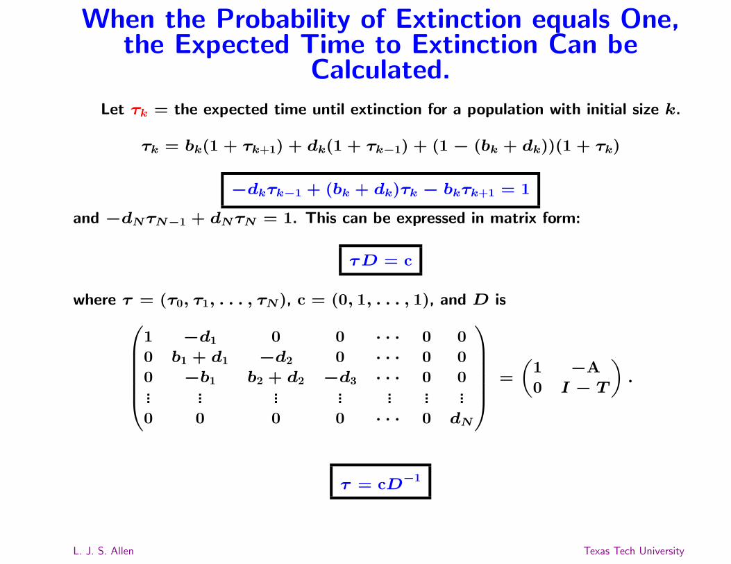
When the Probability of Extinction equals One,the Expected Time to Extinction Can be
Calculated.
Let τk = the expected time until extinction for a population with initial size k.
An Example of a Simple Birth and DeathProcess with N = 20.
Suppose the maximal population size is N = 20, where the birthand death probabilities are linear: bi ≡ 0.03i∆t, for i = 1, 2, . . . , 19,di ≡ 0.02i∆t, for i = 1, 2, . . . , 20, ∆t = 1 a simple birth and deathprocess.
0 5 10 15 200
2
4
6x 10
4
Initial population size
Exp
ecte
d d
ura
tio
n
b > d
Figure 4: Expected time until population extinction τ when the maximumpopulation size is N = 20, bi = 0.03i∆t, and di = 0.02i∆t.
If ∆t = 1 day, 6× 10⁴ ≈ 160 years.
L. J. S. Allen Texas Tech University
(4) SIS Epidemic Model
S I
Deterministic Model:
dS
dt= −
β
NIS + (b + γ)I
dI
dt=β
NIS − (b + γ)I =
β
NI(N − I)− (b + γ)I
S(t) = N − I(t), where N = constant total population size.
Basic Reproduction Number: R0 =β
b+ γ
If R0 ≤ 1, then limt→∞
I(t) = 0.
If R0 > 1, then limt→∞
I(t) = N
(1−
1
R0
)> 0.
L. J. S. Allen Texas Tech University
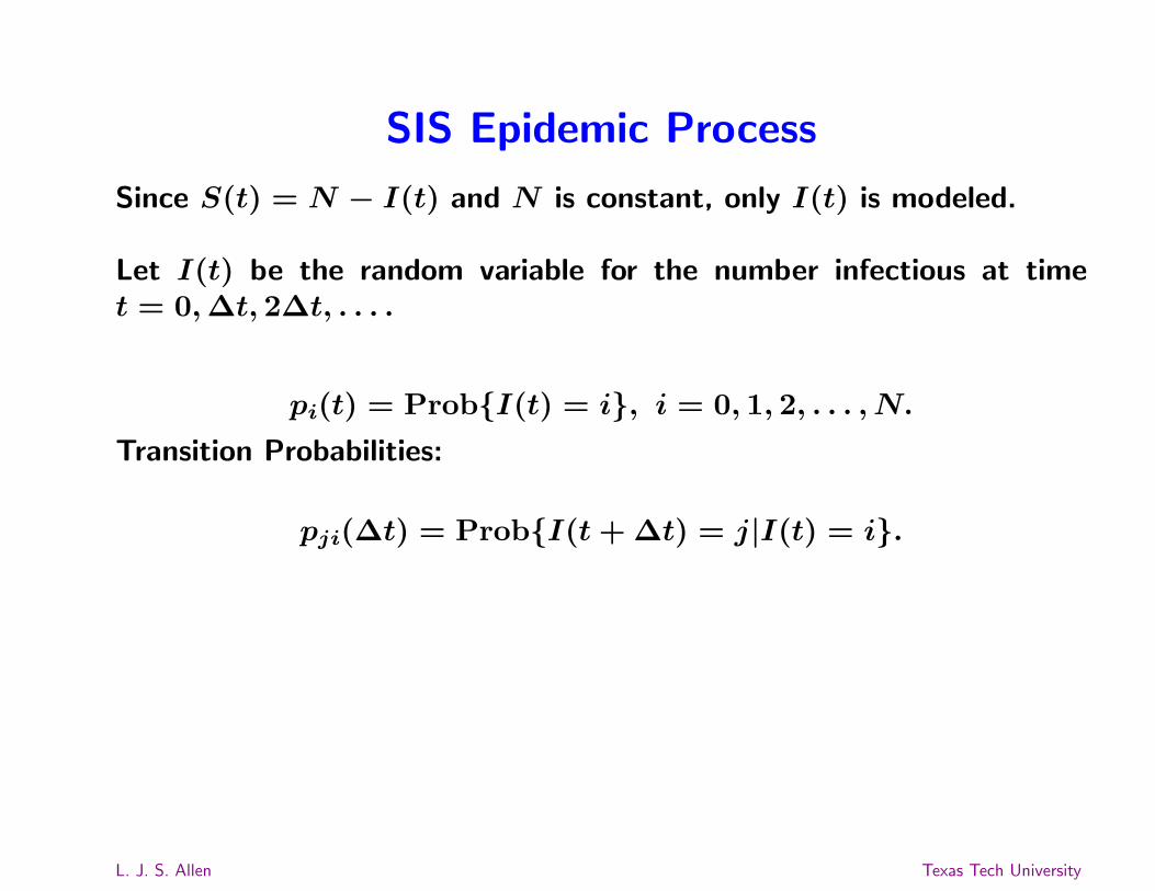
SIS Epidemic Process
Since S(t) = N − I(t) and N is constant, only I(t) is modeled.
Let I(t) be the random variable for the number infectious at timet = 0,∆t, 2∆t, . . . .
pi(t) = Prob{I(t) = i}, i = 0, 1, 2, . . . , N.
Transition Probabilities:
pji(∆t) = Prob{I(t+ ∆t) = j|I(t) = i}.
L. J. S. Allen Texas Tech University
Transition Probabilities
pji(∆t) =
8>>>>>><>>>>>>:
βi(N − i)N
∆t, j = i + 1
(b + γ)i∆t, j = i− 1
1−»βi(N − i)
N+ (b + γ)i
–∆t, j = i
0, j 6= i + 1, i, i− 1.Similar to a birth and death process:
pji(∆t) =
8>><>>:b(i)∆t, j = i + 1d(i)∆t, j = i− 11− [b(i) + d(i)]∆t, j = i
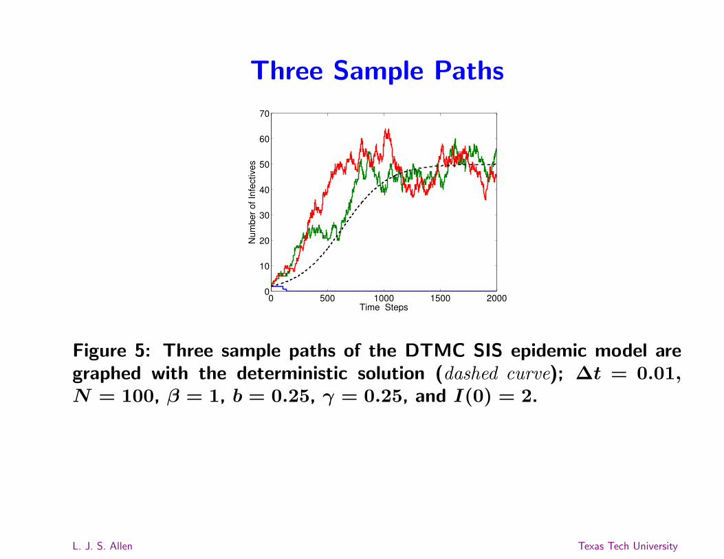
Figure 5: Three sample paths of the DTMC SIS epidemic model aregraphed with the deterministic solution (dashed curve); ∆t = 0.01,N = 100, β = 1, b = 0.25, γ = 0.25, and I(0) = 2.
L. J. S. Allen Texas Tech University
Probability Distribution
025
5075
100
0500
10001500
2000
0
0.25
0.5
0.75
1
InfectivesTime Steps
Prob
abilit
y
Figure 6: Probability distribution of the DTMC SIS epidemic model.∆t = 0.01, N = 100, β = 1, b = 0.25, γ = 0.25, I(0) = 2,R0 = 2. Quasistationary distribution-conditioned on nonextinction,(1/R0)2 = 0.25
See Matlab program.
L. J. S. Allen Texas Tech University
Part II:Discrete-Time Branching Processes (BP)
Single-Type and Multi-Type BP
Single-Type BP: The term “single-type” refers to the fact that allindividuals are of one type such as the same gender, same cell type, orsame genotype or phenotype.
(1) Cell Cycles, Active and Quiescent
Multi-type BP: Instead of only one type, there are several types ofindividuals. A population may be divided according to age, size, ordevelopmental stage, representing different types. In genetics, genesmay be classified as wild or mutant types.
(2) Age-Structured Population
L. J. S. Allen Texas Tech University
Single-Type Galton-Watson BP
In 1873, Galton sent a problem to the Educational Times regardingthe survival of family names. When he did not receive a satisfactoryanswer, he consulted Watson, who rephrased the problem in termsof generating functions. These types of problems are called Galton-Watson BP.
Assumptions:
(i) Each individual in generation n gives birth to Y offspring of the same type, whereY is a discrete random variable. Offspring probabilities:
pj = Prob{Y = j}, j = 0, 1, 2, . . . .
(ii) Each individual in the population gives birth independently of all other individuals.
(iii) The same offspring distribution applies to all generations.
L. J. S. Allen Texas Tech University
A Stochastic Realization or Sample Path of a BP
Let X0 = 1.
0
1
2
3
Figure 7: A sample path or stochastic realization of a branchingprocess {Xn}∞n=0. In the first generation, four individuals are born,X1 = 4. The four individuals give birth to three, zero, four, andone individuals, respectively, making a total of eight individuals ingeneration 2, X2 = 8.
L. J. S. Allen Texas Tech University
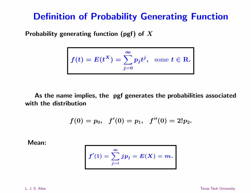
Definition of Probability Generating Function
Probability generating function (pgf) of X
f(t) = E(tX) =∞∑j=0
pjtj, some t ∈ R.
As the name implies, the pgf generates the probabilities associatedwith the distribution
f(0) = p0, f ′(0) = p1, f ′′(0) = 2!p2.
Mean:
f′(1) =
∞Xj=1
jpj = E(X) = m.
L. J. S. Allen Texas Tech University
PGF hn of the Galton-Watson BP Xn
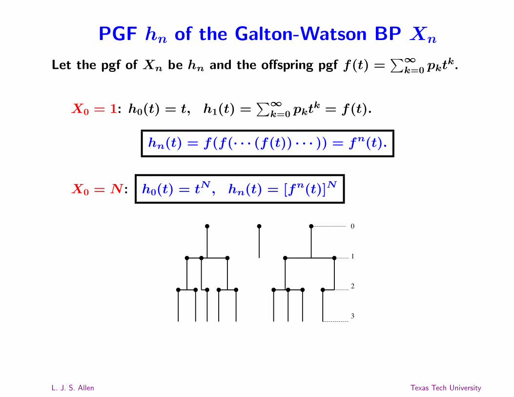
Let the pgf of Xn be hn and the offspring pgf f(t) =∑∞k=0 pkt
k.
X0 = 1: h0(t) = t, h1(t) =∑∞k=0 pkt
k = f(t).
hn(t) = f(f(· · · (f(t)) · · · )) = fn(t).
X0 = N : h0(t) = tN , hn(t) = [fn(t)]N
0
1
2
3
L. J. S. Allen Texas Tech University
Extinction Theorem in Branching Processes.
Theorem 1. Assume X0 = N and the offspring distribution {pk}∞k=0satisfies p0 > 0 and 0 < p0 + p1 < 1.
(i) If m ≤ 1, then
limn→∞
Prob{Xn = 0} = limn→∞
hn(0) = limn→∞
[fn(0)]N = 1
(ii) If m > 1, then there exists unique q < 1 such that f(q) = q
limn→∞
Prob{Xn = 0} = limn→∞
hn(0) = limn→∞
[fn(0)]N = q
L. J. S. Allen Texas Tech University
Extinction in Branching Processes.
The Galton-Watson BP is referred to as supercritical if m > 1,critical if m = 1, and subcritical if m < 1.
If the process is subcritical or critical, then the probability ofextinction is certain.
But if the process is supercritical, then there is a positive probability,1− qN , that the population will survive. As the initial population sizeincreases, the probability of survival also increases.
L. J. S. Allen Texas Tech University
(1) Cell Cycle: Active and Quiescent
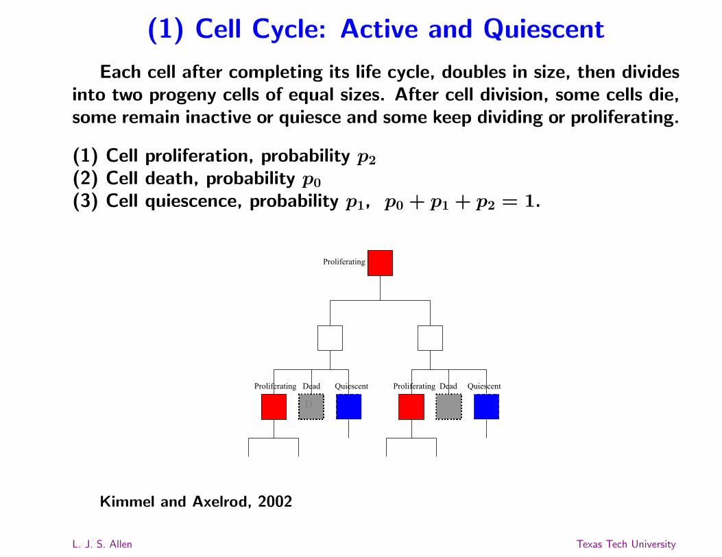
Each cell after completing its life cycle, doubles in size, then dividesinto two progeny cells of equal sizes. After cell division, some cells die,some remain inactive or quiesce and some keep dividing or proliferating.
Proliferating Dead Quiescent Proliferating Dead Quiescent
D
Kimmel and Axelrod, 2002
L. J. S. Allen Texas Tech University
The Cell Cycle is a Galton-Watson Process
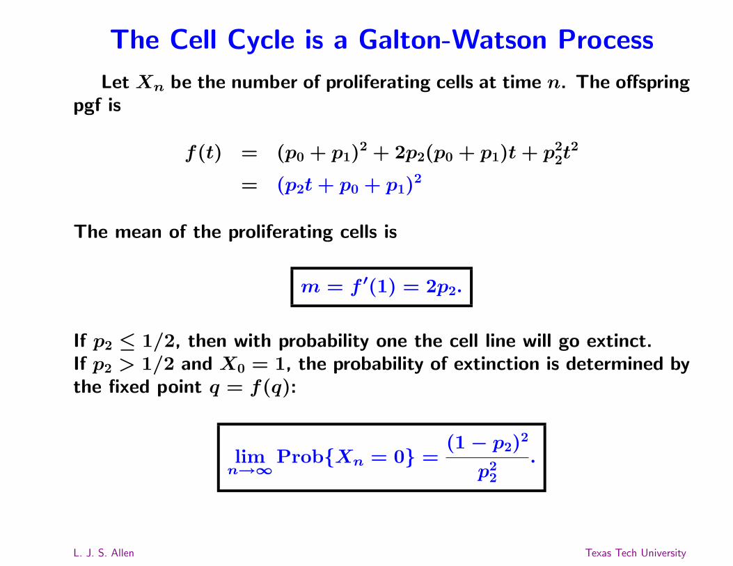
Let Xn be the number of proliferating cells at time n. The offspringpgf is
f(t) = (p0 + p1)2 + 2p2(p0 + p1)t+ p22t
2
= (p2t+ p0 + p1)2
The mean of the proliferating cells is
m = f ′(1) = 2p2.
If p2 ≤ 1/2, then with probability one the cell line will go extinct.If p2 > 1/2 and X0 = 1, the probability of extinction is determined bythe fixed point q = f(q):
limn→∞
Prob{Xn = 0} =(1− p2)2
p22
.
L. J. S. Allen Texas Tech University
Multi-type Galton Watson BP
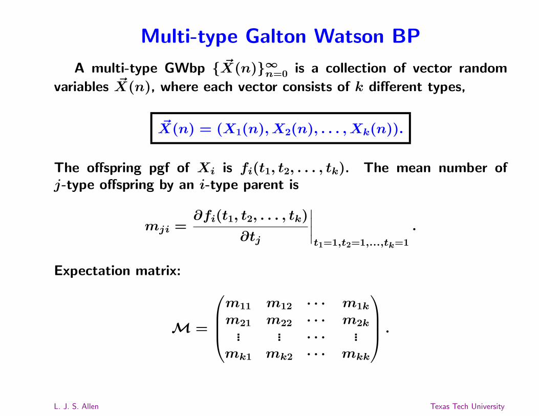
A multi-type GWbp { ~X(n)}∞n=0 is a collection of vector random
variables ~X(n), where each vector consists of k different types,
~X(n) = (X1(n), X2(n), . . . , Xk(n)).
The offspring pgf of Xi is fi(t1, t2, . . . , tk). The mean number ofj-type offspring by an i-type parent is
mji =∂fi(t1, t2, . . . , tk)
∂tj
∣∣∣∣t1=1,t2=1,...,tk=1
.
Expectation matrix:
M =
m11 m12 · · · m1k
m21 m22 · · · m2k... ... · · · ...
mk1 mk2 · · · mkk
.
L. J. S. Allen Texas Tech University
Extinction Theorem for Multi-typeGalton-Watson BP
Theorem 2. Let the initial sizes for each type be Xi(0) = Ni,i = 1, 2, . . . , k. Suppose the generating functions fi for each of the ktypes are nonlinear functions of tj with some fi(0, 0, . . . , 0) > 0, theexpectation matrix M is regular, and λ is the dominant eigenvalueof matrix M.(i) If λ ≤ 1, then the probability of ultimate extinction is one,
limn→∞
Prob{ ~X(n) = ~0} = 1.
(ii) If λ > 1, then the probability of ultimate extinction is less thanone,
limn→∞
Prob{ ~X(n) = ~0} = qN11 qN2
2 · · · qNkk ,
where (q1, q2, . . . , qk) is the unique fixed point of the k generatingfunctions fi(q1, . . . , qk) = qi and 0 < qi < 1, i = 1, 2 . . . , k.
L. J. S. Allen Texas Tech University
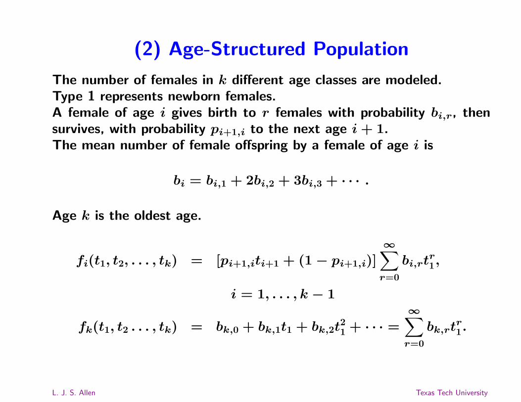
(2) Age-Structured Population
The number of females in k different age classes are modeled.Type 1 represents newborn females.A female of age i gives birth to r females with probability bi,r, thensurvives, with probability pi+1,i to the next age i+ 1.The mean number of female offspring by a female of age i is