TV-regularized Iterative Image Reconstruction on a Mobile C-ARM CT

Yongsheng Pan, Ross Whitaker1 and Arvi Cheryauka, Dave Ferguson2

1Scientific Computing and Imaging Institute, University of Utah, 72 South Central

Campus Drive, 3750 WEB, Salt Lake City, UT, 84112, USA 2GE Healthcare - Surgery, 384 Wright Brothers Drive, Salt Lake City, UT, 84116

ABSTRACT

3D computed tomography has been extensively studied and widely used in modern society. Although most manufacturers choose the filtered backprojection algorithm (FBP) for its accuracy and efficiency, iterative reconstruction methods have a significant potential to provide superior performance for incomplete, noisy projection data. However, iterative methods have a high computational cost, which hinders their practical use. Furthermore, regularization is usually required to reduce the effects of noise. In this paper, we analyze the use of the Simultaneous Algebraic Reconstruction Technique (SART) with total variation (TV) regularization. Additionally, graphics hardware is utilized to increase the speed of SART. NVIDIA’s GPU and Compute Unified Device Architecture (CUDA) comprise the core of our computational platform. GPU implementation details, including ray-based forward projection and voxel-based backprojection are illustrated. Experimental results for high-resolution synthetic and real data are provided to demonstrate the accuracy and efficiency of the proposed framework. 1 Keywords: C-arm CT, FDK, SART, TV, GPU, CUDA 1. INTRODUCTION Computed tomography (CT) has been extensively studied and widely used for a variety of medical applications. CT reconstruction methods can be roughly categorized as analytical reconstruction methods such as filtered backprojection (FBP) methods and optimization-based iterative reconstruction methods such as algebraic methods.

Reconstruction by filtered backprojection (FBP) is used by most manufacturers because of speed, ease of implementation and relatively few parameters. In practice, an FBP algorithm, specifically designed to approximate 3D cone beam geometries, proposed by Feldkamp et al [2], is widely used. FBP methods, however, require sufficient projection data with low noise level. This, combined with the approximations used for cone-beam acquisions, results in reconstruction artifacts. Iterative reconstruction methods, such as simultaneous algebraic reconstruction technique (SART), have a significant potential to provide superior performance with incomplete and noisy data, or with less than ideal geometries such as cone-beam systems. Algebraic reconstruction methods require less data than FBP methods [3], and they are more robust to the effects of noise. Furthermore, these methods can include nonlinear regularization terms, which are analogous to the linear filters used in FBP. However, the iterative nature of algebraic methods poses a computational challenge, and the requirement

Further author information: (Send correspondence to Ross Whitaker) Ross Whitaker: Email: whitaker@cs.utah.edu. Telephone: 1 801 587 9549 Arvi Cheryauka: Emal: Arvi.Cheryauka@med.ge.com. Telephone: 1 801 536 4653

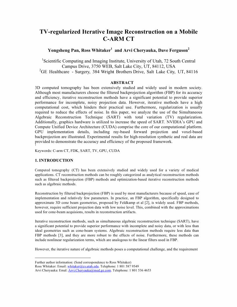
(a) (b) (c) Figure 1. Illustration of FBP reconstruction. (a) Original synthetic 2D image. (b) Projection of (a) using equidistant fan beam. (c) FBP reconstruction using (b). of the regularization of the solutions further increases the computation time. Many improvements on algebraic methods [4-9, 16] have been proposed recently. The methods proposed in [4, 5, 7] apply regularization methods to image reconstruction. The methods in [8, 9] utilize graphics processing unit (GPU) to speed up the SART method. However, few of them address GPU and regularization together to improve iterative methods. On the other hand, while Cg [10] is applied in [8] and OpenGL texture mapping [11] is utilized in [9] for speed-up, both platforms are nontrivial to implement. The recently proposed API for graphics cards, called compute unified device architecture (CUDA), is more general for GPU computing. The simultaneous algebraic reconstruction technique (SART) is studied in this paper, while the Feldkamp method (FDK) for filtered backprojection may be used as an initialization for iterative SART. Graphics hardware is utilized to increase the speed of SART implementation. Nvidia processors and CUDA form the platform for GPU computation. Furthermore, we use total variation (TV) minimization to regularize the SART algorithm. GPU SART reconstruction results for both synthetic and real data are presented. This paper is organized as follows. Section 2 introduces the background information. The proposed framework and its implementation details are shown in Section 3. Experimental results are provided in Section 4. Section 5 contains the summary and the discussions for future work. 2. BACKGROUND This section provides background information on FBP, SART, and TV algorithms. These algorithms form the framework utilized in Section 3. 2.1 FBP FBP methods reconstruct an object using Fourier transforms. They generally entail three steps. First, the Fourier transform

!

S(w) for each projection

!

P(t) is calculated. Second, the Fourier transform

!

S(w) is multiplied with the weighting function

!

2" # K in the frequency domain, where

!

" # $"m,"m[ ] represents the bandlimited frequency and

!

K is the number of projections.

!

"m is the maximum frequency related to the sampling interval during data acquisition. This step is usually implemented by a convolution in the time domain. Third, the inverse Fourier transforms of the filtered projections are summarized over the image plane, which is called the backprojection process. Reconstruction results from FBP methods are affected by the imaging beam types: parallel beam, equiangular fan beam and equidistant fan beam. Fig. 1 shows an example of FBP reconstruction of a 2D object using the projections from the equidistant fan beam. It can be seen in Fig. 1 (c) that the reconstruction is good except for some artifacts in the background.

Three-dimensional cone beam geometry is a 3D generalization of the 2D equidistant fan beam geometry, and results when a 3D object is irradiated with a point source and the signal intensity is measured on a detector plane. The Feldkamp algorithm (FDK) [2] is a practical FBP algorithm designed for 3D cone beam reconstruction. It is fast to compute, but only approximate, and it results in reconstruction artifacts off the center axis. 2.2 SART Algebraic methods formulate the reconstruction problem as finding an array of unknowns using algebraic equations from the projection data. These methods are designed to solve the following simultaneous equation system where

!

pi represents the

!

i th projection,

!

wij represents the weight which the voxel

!

v j contributes its value to the

!

i th projection. Reconstruction is achieved by finding

!

v j from the equation system (1). The SART algorithm solves the equation system by iteratively applying a correction array to each voxel

!

v j as follows

where

!

" is a constant coefficient. It has been proved that the SART algorithm converges globally to the solution of a weighted least square problem for

!

" # (0,2) [12]. An initial condition for the reconstruction

!

v j needs to be specified for iterative updates in the implementation. 2.3 Total Variation Minimization Total variation minimization [13] is a nonlinear image denoising method that performs a gradient descent on the total variation of the image. Given an image

!

f defined on domain

!

", this method seeks a regularized image

!

u which minimizes the following energy functional where

!

" is a constant coefficient. This energy functional has the nice property of allowing (or preserving) straight, sharp edges, and thus allows solutions to have a piecewise flat property. It has been, very recently, tied to the more general method of compressed sensing [14]. The minimization of the energy function (3) is numerically calculated using the following update scheme

!

F(u) = "u +#

2u $ f

2

%&

%&

!

pi = wijvjj=1

N

"

!

vjk+1

= vjk+ "

wij

pi # wimvmk

m=1

N

$

wim

m=1

N

$

%

&

' '

(

' '

)

*

' '

+

' '

i

$

wij

i

$ (2)

(3)

!

un+1" un

#t= $%

$un

$un" &(un " f ) (4)

(1)

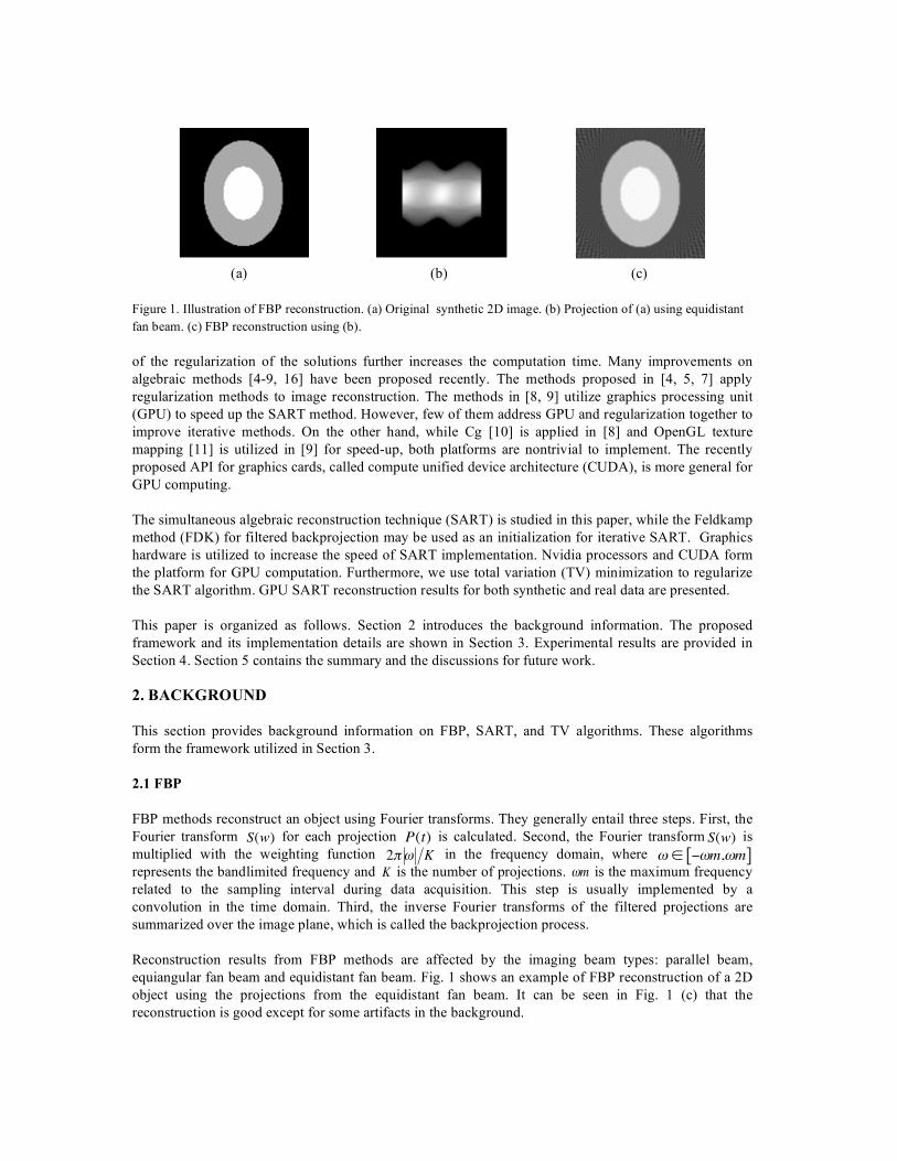
(a) (b) (c) Figure 2. Illustration of TV regularization. (a) Original image with noise. (b) Image regularized using TV with

!

" = 0.1. (c) Image regularized using TV with

!

" = 0.5 . where

!

"t represents the time step and

!

un

is the image value for iteration

!

n . The minimization is iteratively processed until convergence is achieved. Fig. 2 illustrates the regularization effects of TV. Fig. 2(b) shows the TV results from the original image Fig. 2(a) with the coefficient

!

" = 0.1, and Fig. 2(c) shows the results with the coefficient

!

" = 0.5 . It can be seen that the TV results contain less noise than the original image and that the results in Fig. 2(c) are closer to the original image with larger

!

" . 3. PROPOSED FRAMEWORK AND GPU IMPLEMENTATION DETAILS FDK, SART and TV methods introduced above may be combined for 3D CT reconstruction, depending on applications. Although SART is proved to converge, the initialization may make a difference on efficiency. The reconstruction results from FDK may be utilized as an initialization for SART for this aspect while its initialization can be generally set to be zero. The TV method is applied after each iteration of SART to reduce the effects of noise. This framework takes the following steps for algebraic reconstruction.

• Step 1. Perform FDK reconstruction for SART initialization (optional). • Step 2. Perform TV on FDK results using (4) (optional). • Step 3. Compute forward projection and compute correction image for each ray, i.e., • Step 4. Compute backward projection and update each voxel, i.e.,

• Step 5. Perform TV on SART results using (4). where steps 3-5 are iterated until convergence is achieved. The above framework is implemented using both CPU and GPU. The CPU implementation is relatively

!

ˆ p i = wimvm

k

m =1

N

"

!

"ri = pi # ˆ p i( ) wim

m=1

N

$

!

v j

k+1= v j

k+ "

wij#rii

$

wij

i

$

Figure 3. Ray-based forward projection mechanism with an equidistant sample step size. straightforward, but it usually requires the storage of huge weight information {

!

wij } for efficiency. For an object of size 256

!

"256

!

"193 and projections of size 100

!

"339

!

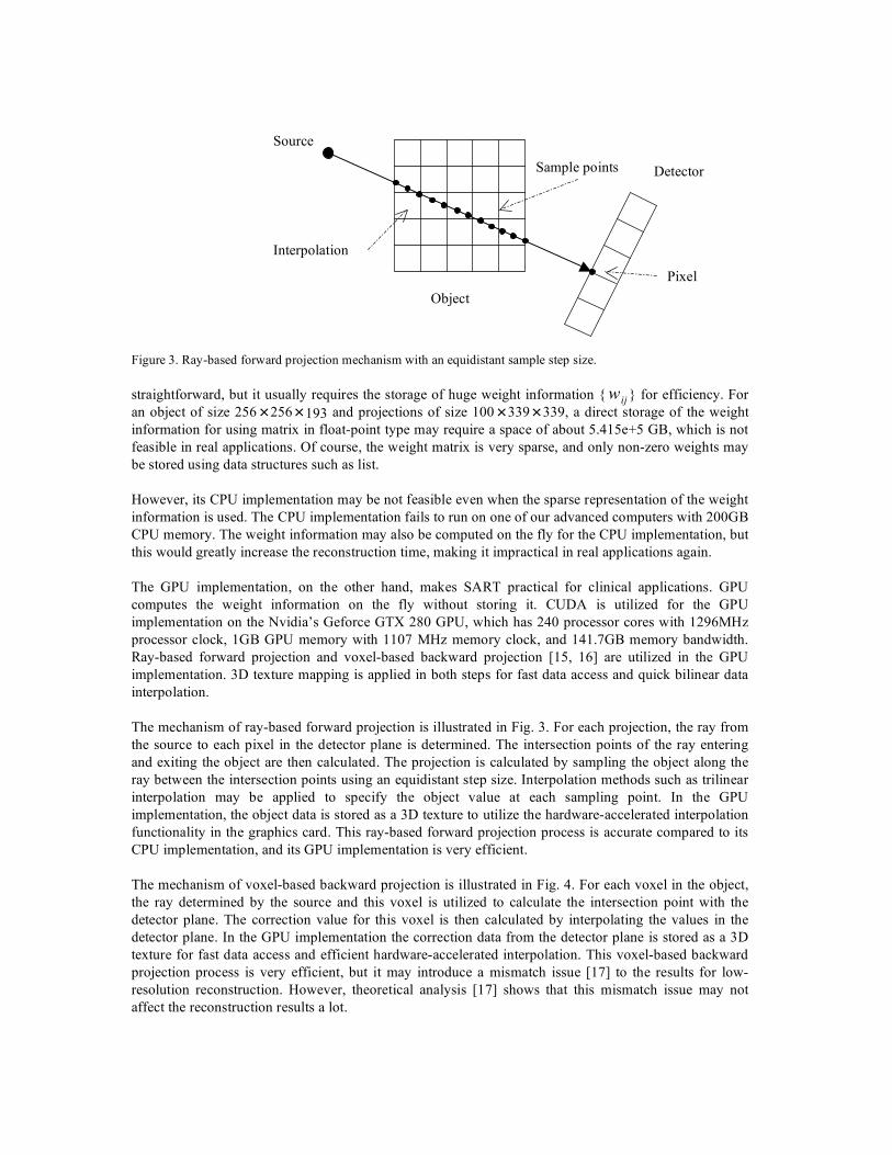
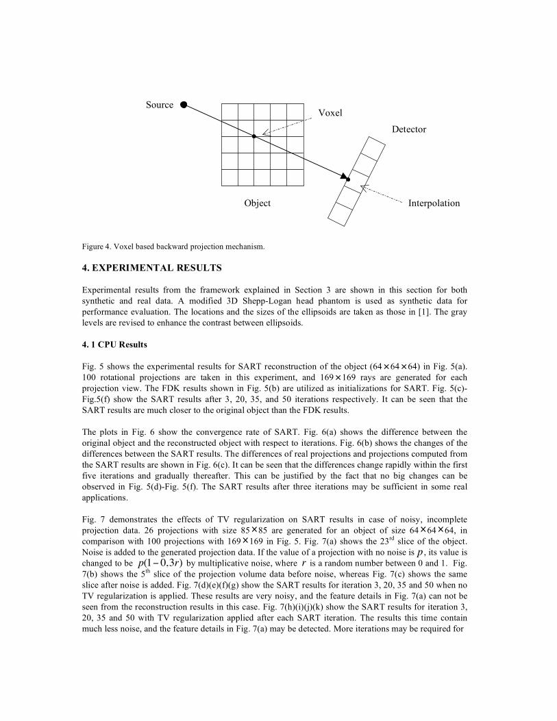
"339, a direct storage of the weight information for using matrix in float-point type may require a space of about 5.415e+5 GB, which is not feasible in real applications. Of course, the weight matrix is very sparse, and only non-zero weights may be stored using data structures such as list. However, its CPU implementation may be not feasible even when the sparse representation of the weight information is used. The CPU implementation fails to run on one of our advanced computers with 200GB CPU memory. The weight information may also be computed on the fly for the CPU implementation, but this would greatly increase the reconstruction time, making it impractical in real applications again. The GPU implementation, on the other hand, makes SART practical for clinical applications. GPU computes the weight information on the fly without storing it. CUDA is utilized for the GPU implementation on the Nvidia’s Geforce GTX 280 GPU, which has 240 processor cores with 1296MHz processor clock, 1GB GPU memory with 1107 MHz memory clock, and 141.7GB memory bandwidth. Ray-based forward projection and voxel-based backward projection [15, 16] are utilized in the GPU implementation. 3D texture mapping is applied in both steps for fast data access and quick bilinear data interpolation. The mechanism of ray-based forward projection is illustrated in Fig. 3. For each projection, the ray from the source to each pixel in the detector plane is determined. The intersection points of the ray entering and exiting the object are then calculated. The projection is calculated by sampling the object along the ray between the intersection points using an equidistant step size. Interpolation methods such as trilinear interpolation may be applied to specify the object value at each sampling point. In the GPU implementation, the object data is stored as a 3D texture to utilize the hardware-accelerated interpolation functionality in the graphics card. This ray-based forward projection process is accurate compared to its CPU implementation, and its GPU implementation is very efficient. The mechanism of voxel-based backward projection is illustrated in Fig. 4. For each voxel in the object, the ray determined by the source and this voxel is utilized to calculate the intersection point with the detector plane. The correction value for this voxel is then calculated by interpolating the values in the detector plane. In the GPU implementation the correction data from the detector plane is stored as a 3D texture for fast data access and efficient hardware-accelerated interpolation. This voxel-based backward projection process is very efficient, but it may introduce a mismatch issue [17] to the results for low-resolution reconstruction. However, theoretical analysis [17] shows that this mismatch issue may not affect the reconstruction results a lot.

Source

Object

Detector Sample points

Interpolation

Pixel

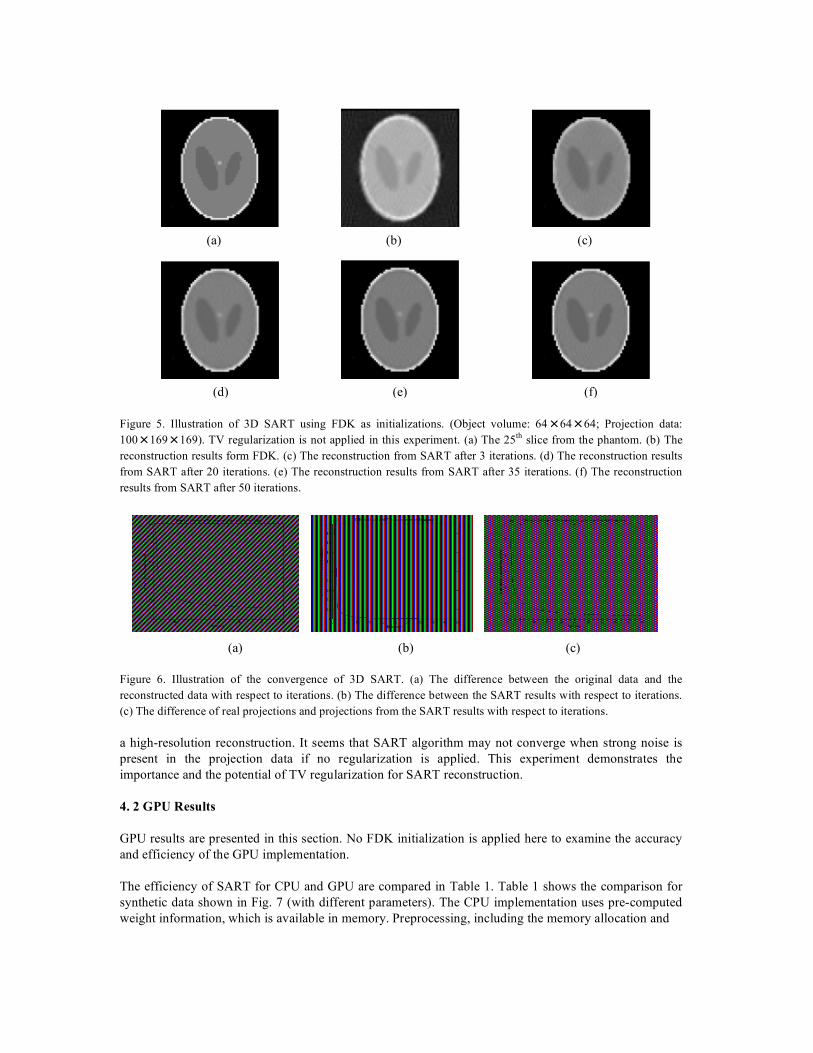
Figure 4. Voxel based backward projection mechanism. 4. EXPERIMENTAL RESULTS Experimental results from the framework explained in Section 3 are shown in this section for both synthetic and real data. A modified 3D Shepp-Logan head phantom is used as synthetic data for performance evaluation. The locations and the sizes of the ellipsoids are taken as those in [1]. The gray levels are revised to enhance the contrast between ellipsoids. 4. 1 CPU Results Fig. 5 shows the experimental results for SART reconstruction of the object (64

!

"64

!

"64) in Fig. 5(a). 100 rotational projections are taken in this experiment, and 169

!

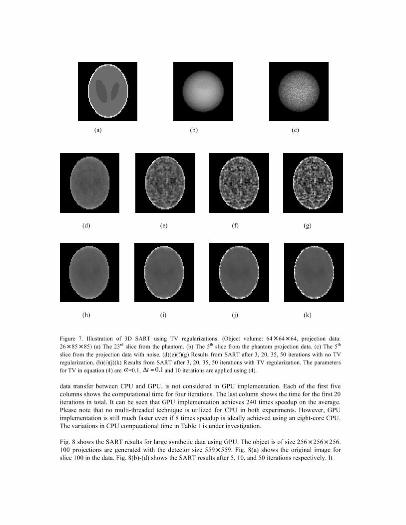
"169 rays are generated for each projection view. The FDK results shown in Fig. 5(b) are utilized as initializations for SART. Fig. 5(c)-Fig.5(f) show the SART results after 3, 20, 35, and 50 iterations respectively. It can be seen that the SART results are much closer to the original object than the FDK results. The plots in Fig. 6 show the convergence rate of SART. Fig. 6(a) shows the difference between the original object and the reconstructed object with respect to iterations. Fig. 6(b) shows the changes of the differences between the SART results. The differences of real projections and projections computed from the SART results are shown in Fig. 6(c). It can be seen that the differences change rapidly within the first five iterations and gradually thereafter. This can be justified by the fact that no big changes can be observed in Fig. 5(d)-Fig. 5(f). The SART results after three iterations may be sufficient in some real applications. Fig. 7 demonstrates the effects of TV regularization on SART results in case of noisy, incomplete projection data. 26 projections with size 85

!

"85 are generated for an object of size 64

!

"64

!

"64, in comparison with 100 projections with 169

!

"169 in Fig. 5. Fig. 7(a) shows the 23rd slice of the object. Noise is added to the generated projection data. If the value of a projection with no noise is

!

p , its value is changed to be

!

p(1" 0,3r) by multiplicative noise, where

!

r is a random number between 0 and 1. Fig. 7(b) shows the 5th slice of the projection volume data before noise, whereas Fig. 7(c) shows the same slice after noise is added. Fig. 7(d)(e)(f)(g) show the SART results for iteration 3, 20, 35 and 50 when no TV regularization is applied. These results are very noisy, and the feature details in Fig. 7(a) can not be seen from the reconstruction results in this case. Fig. 7(h)(i)(j)(k) show the SART results for iteration 3, 20, 35 and 50 with TV regularization applied after each SART iteration. The results this time contain much less noise, and the feature details in Fig. 7(a) may be detected. More iterations may be required for

Source

Object

Detector Voxel

Interpolation

Figure 5. Illustration of 3D SART using FDK as initializations. (Object volume: 64

!

"64

!

"64; Projection data: 100

!

"169

!

"169). TV regularization is not applied in this experiment. (a) The 25th slice from the phantom. (b) The reconstruction results form FDK. (c) The reconstruction from SART after 3 iterations. (d) The reconstruction results from SART after 20 iterations. (e) The reconstruction results from SART after 35 iterations. (f) The reconstruction results from SART after 50 iterations.

Figure 6. Illustration of the convergence of 3D SART. (a) The difference between the original data and the reconstructed data with respect to iterations. (b) The difference between the SART results with respect to iterations. (c) The difference of real projections and projections from the SART results with respect to iterations. a high-resolution reconstruction. It seems that SART algorithm may not converge when strong noise is present in the projection data if no regularization is applied. This experiment demonstrates the importance and the potential of TV regularization for SART reconstruction. 4. 2 GPU Results GPU results are presented in this section. No FDK initialization is applied here to examine the accuracy and efficiency of the GPU implementation. The efficiency of SART for CPU and GPU are compared in Table 1. Table 1 shows the comparison for synthetic data shown in Fig. 7 (with different parameters). The CPU implementation uses pre-computed weight information, which is available in memory. Preprocessing, including the memory allocation and

(a) (b) (c)

(d) (e) (f)

(a)

(b)

(c)

Figure 7. Illustration of 3D SART using TV regularizations. (Object volume: 64

!

"64

!

"64, projection data: 26

!

"85

!

"85) (a) The 23rd slice from the phantom. (b) The 5th slice from the phantom projection data. (c) The 5th slice from the projection data with noise. (d)(e)(f)(g) Results from SART after 3, 20, 35, 50 iterations with no TV regularization. (h)(i)(j)(k) Results from SART after 3, 20, 35, 50 iterations with TV regularization. The parameters for TV in equation (4) are

!

"=0.1,

!

"t = 0.1 and 10 iterations are applied using (4). data transfer between CPU and GPU, is not considered in GPU implementation. Each of the first five columns shows the computational time for four iterations. The last column shows the time for the first 20 iterations in total. It can be seen that GPU implementation achieves 240 times speedup on the average. Please note that no multi-threaded technique is utilized for CPU in both experiments. However, GPU implementation is still much faster even if 8 times speedup is ideally achieved using an eight-core CPU. The variations in CPU computational time in Table 1 is under investigation. Fig. 8 shows the SART results for large synthetic data using GPU. The object is of size 256

!

"256

!

"256. 100 projections are generated with the detector size 559

!

"559. Fig. 8(a) shows the original image for slice 100 in the data. Fig. 8(b)-(d) shows the SART results after 5, 10, and 50 iterations respectively. It

(a)

(b)

(c)

(d)

(e)

(f)

(g)

(h) (i) (j) (k)

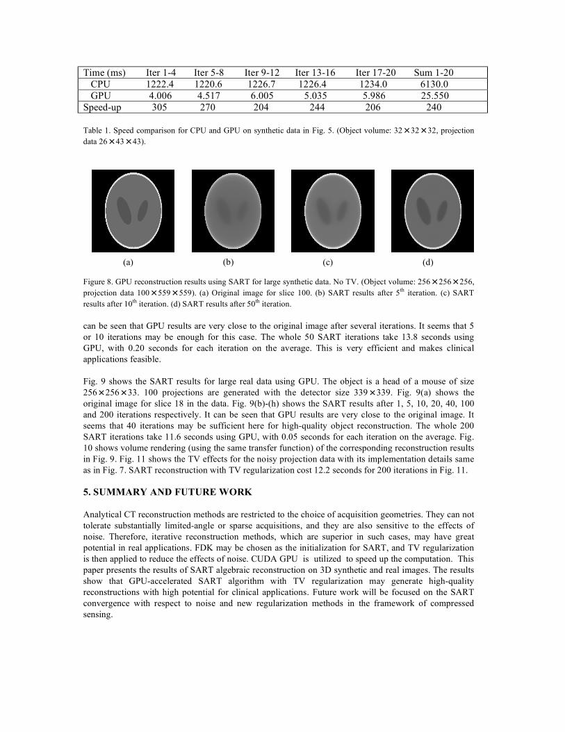
Time (ms) Iter 1-4 Iter 5-8 Iter 9-12 Iter 13-16 Iter 17-20 Sum 1-20 CPU 1222.4 1220.6 1226.7 1226.4 1234.0 6130.0 GPU 4.006 4.517 6.005 5.035 5.986 25.550 Speed-up 305 270 204 244 206 240 Table 1. Speed comparison for CPU and GPU on synthetic data in Fig. 5. (Object volume: 32

!

"32

!

"32, projection data 26

!

"43

!

"43).

Figure 8. GPU reconstruction results using SART for large synthetic data. No TV. (Object volume: 256

!

"256

!

"256, projection data 100

!

"559

!

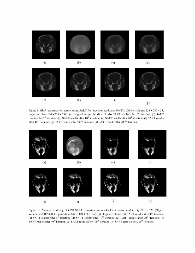
"559). (a) Original image for slice 100. (b) SART results after 5th iteration. (c) SART results after 10th iteration. (d) SART results after 50th iteration. can be seen that GPU results are very close to the original image after several iterations. It seems that 5 or 10 iterations may be enough for this case. The whole 50 SART iterations take 13.8 seconds using GPU, with 0.20 seconds for each iteration on the average. This is very efficient and makes clinical applications feasible. Fig. 9 shows the SART results for large real data using GPU. The object is a head of a mouse of size 256

!

"256

!

"33. 100 projections are generated with the detector size 339

!

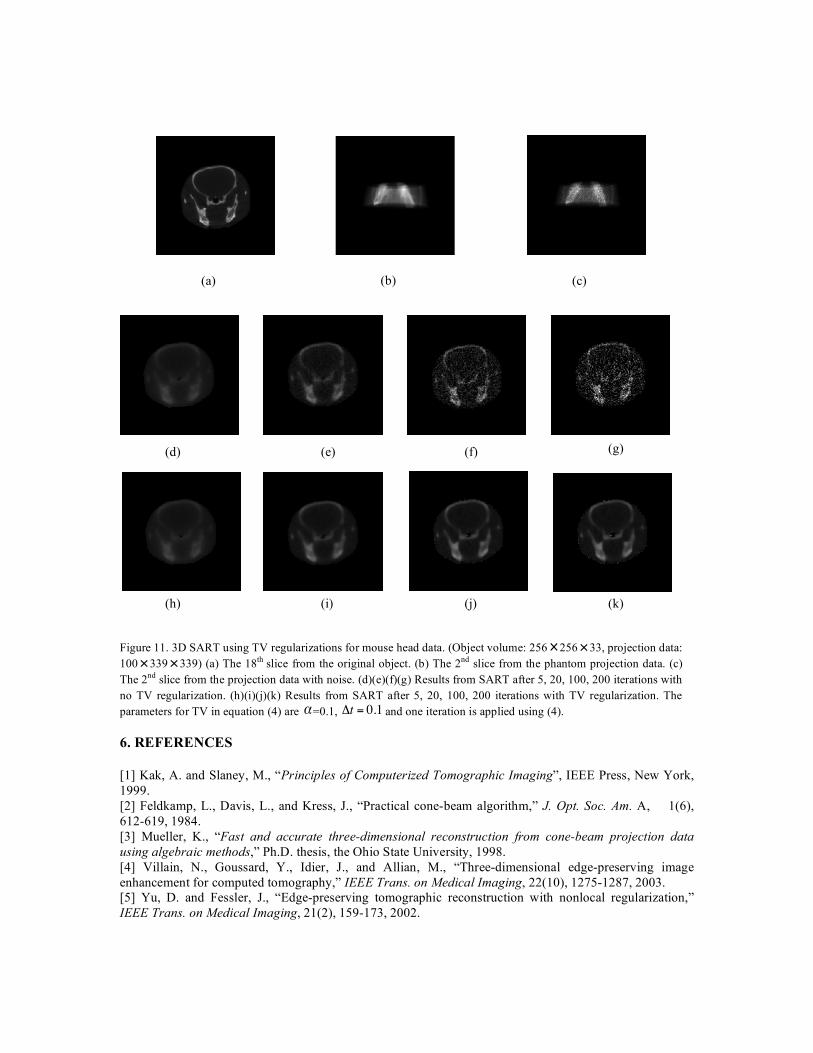
"339. Fig. 9(a) shows the original image for slice 18 in the data. Fig. 9(b)-(h) shows the SART results after 1, 5, 10, 20, 40, 100 and 200 iterations respectively. It can be seen that GPU results are very close to the original image. It seems that 40 iterations may be sufficient here for high-quality object reconstruction. The whole 200 SART iterations take 11.6 seconds using GPU, with 0.05 seconds for each iteration on the average. Fig. 10 shows volume rendering (using the same transfer function) of the corresponding reconstruction results in Fig. 9. Fig. 11 shows the TV effects for the noisy projection data with its implementation details same as in Fig. 7. SART reconstruction with TV regularization cost 12.2 seconds for 200 iterations in Fig. 11. 5. SUMMARY AND FUTURE WORK Analytical CT reconstruction methods are restricted to the choice of acquisition geometries. They can not tolerate substantially limited-angle or sparse acquisitions, and they are also sensitive to the effects of noise. Therefore, iterative reconstruction methods, which are superior in such cases, may have great potential in real applications. FDK may be chosen as the initialization for SART, and TV regularization is then applied to reduce the effects of noise. CUDA GPU is utilized to speed up the computation. This paper presents the results of SART algebraic reconstruction on 3D synthetic and real images. The results show that GPU-accelerated SART algorithm with TV regularization may generate high-quality reconstructions with high potential for clinical applications. Future work will be focused on the SART convergence with respect to noise and new regularization methods in the framework of compressed sensing.

(a)

(b) (c)

(d)

Figure 9. GPU reconstruction results using SART for large real head data. No TV. (Object volume: 256

!

"256

!

"33, projection data 100

!

"339

!

"339). (a) Original image for slice 18. (b) SART results after 1st iteration. (c) SART results after 5th iteration. (d) SART results after 10th iteration. (e) SART results after 20th iteration. (f) SART results after 40th iteration. (g) SART results after 100th iteration. (h) SART results after 200th iteration. Figure 10. Volume rendering of GPU SART reconstruction results for a mouse head in Fig. 9. No TV. (Object volume: 256

!

"256

!

"33, projection data 100

!

"339

!

"339). (a) Original volume. (b) SART results after 1st iteration. (c) SART results after 5st iteration. (d) SART results after 10th iteration. (e) SART results after 20th iteration. (f) SART results after 40th iteration. (g) SART results after 100th iteration. (h) SART results after 200th iteration.

(a) (b) (c) (d)

(e) (f) (g)

(h)

(a)

(b)

(c)

(d)

(e) (f) (g) (h)

Figure 11. 3D SART using TV regularizations for mouse head data. (Object volume: 256

!

"256

!

"33, projection data: 100

!

"339

!

"339) (a) The 18th slice from the original object. (b) The 2nd slice from the phantom projection data. (c) The 2nd slice from the projection data with noise. (d)(e)(f)(g) Results from SART after 5, 20, 100, 200 iterations with no TV regularization. (h)(i)(j)(k) Results from SART after 5, 20, 100, 200 iterations with TV regularization. The parameters for TV in equation (4) are

!

"=0.1,

!

"t = 0.1 and one iteration is applied using (4). 6. REFERENCES [1] Kak, A. and Slaney, M., “Principles of Computerized Tomographic Imaging”, IEEE Press, New York, 1999. [2] Feldkamp, L., Davis, L., and Kress, J., “Practical cone-beam algorithm,” J. Opt. Soc. Am. A, 1(6), 612-619, 1984. [3] Mueller, K., “Fast and accurate three-dimensional reconstruction from cone-beam projection data using algebraic methods,” Ph.D. thesis, the Ohio State University, 1998. [4] Villain, N., Goussard, Y., Idier, J., and Allian, M., “Three-dimensional edge-preserving image enhancement for computed tomography,” IEEE Trans. on Medical Imaging, 22(10), 1275-1287, 2003. [5] Yu, D. and Fessler, J., “Edge-preserving tomographic reconstruction with nonlocal regularization,” IEEE Trans. on Medical Imaging, 21(2), 159-173, 2002.

(a)

(b) (c)

(d)

(e)

(f)

(g)

(h) (i) (j) (k)

[6] Hsieh, J. and Tang, X., “Tilted cone-beam reconstruction with row-wise fan-to-parallel rebinning,” Physics in Medicine and Biology, 51, 5259-5276, 2006. [7] Sidky, E. and Pan, X., “Few-view, cone-beam CT image reconstruction by GPU-accelerated total variation minimization,” in 9th International Meeting on Fully Three-Dimensional Image Reconstruction in Radiology and Nuclear Medicine, Kacheriess, M., Beekman, F., and Mueller, K., eds., 60-63, 2007. [8] Tita, R. and Lueth, T., “Online iterative reconstruction with the use of the Graphical Processing Unit (GPU),” in 9th International Meeting on Fully Three-Dimensional Image Reconstruction in Radiology and Nuclear Medicine, Kacheriess, M., Beekman, F., and Mueller, K., eds., 72-75, 2007. [9] Mueller, K. and Yagel, R., “Rapid 3-D reconstruction with the Simultaneous Algebraic Reconstruction Technique (SART) using 2-D texture mapping hardware,” IEEE Trans. on Medical Imaging, 19(12), 1227-1237, 2000. [10] Fernando, R. and Kilgard, M., “The Cg Tutorial: The Definitive Guide to Programmable Real-Time Graphics”, Addision-Wesley Professional, March 2003. [11] Shreiner, D., Woo, M., Neider, J., and Davis, T., “OpenGL Programming Guide”, Addison-Wesley Professional, 5 ed., 2006. [12] Jiang, M. and Wang, G., “Convergence of the Simultaneous Algebraic Reconstruction Technique (SART),” IEEE Trans. on Image Processing, 12 (8), 957-961, Aug. 2003. [13] Rudin, L. I., Osher, S., and Fatemi, E., “Nonlinear total variation based noise removal algorithms,” Physica D, 60, 259-268, 1992. [14] Candes, E., Romberg, J., and Tao, T., “Robust uncertainty principles: Exact signal reconstruction from highly incomplete frequency information,” IEEE Trans. on Information Theory, 52, 489-509, 2006. [15] Galigekere, R. R., Wiesent, K., and Holdsworth D. W., “Cone-beam reprojection using projection-matrices,” IEEE Trans. on Medical Imaging, 22(10), 1202-1214, Oct. 2003. [16] Keck, B., Hofmann, H., Scherl H., Kowarschik M., and Hornegger J., “GPU-accelerated SART reconstruction using the CUDA programming environment,” Proc. SPIE, vol. 7258, 72582B, 2009. [17] Man, B. D., and Basu, S., “Distance-driven projection and backprojection in three dimensions,” Physics in Medicine and Biology, 49, 2463-2475, 2004. [18] Pan, Y., Whitaker, R., Cheryauka, A., Ferguson D., “Feasibility of GPU-assisted iterative image reconstruction for mobile C-arm CT,” Proc. SPIE, vol. 7258, 72585J, 2009.