Two and threeparticle distribution functions for lattice fluids fromOrnstein–Zernike equationsElijah Johnson Citation: J. Chem. Phys. 86, 5739 (1987); doi: 10.1063/1.452501 View online: http://dx.doi.org/10.1063/1.452501 View Table of Contents: http://jcp.aip.org/resource/1/JCPSA6/v86/i10 Published by the AIP Publishing LLC. Additional information on J. Chem. Phys.Journal Homepage: http://jcp.aip.org/ Journal Information: http://jcp.aip.org/about/about_the_journal Top downloads: http://jcp.aip.org/features/most_downloaded Information for Authors: http://jcp.aip.org/authors

Downloaded 07 Oct 2013 to 128.123.35.41. This article is copyrighted as indicated in the abstract. Reuse of AIP content is subject to the terms at: http://jcp.aip.org/about/rights_and_permissions

Two- and three-particle distribution functions for lattice fluids from Ornstein­Zernike equations8

)

Elijah Johnson Chemistry Division, Oak Ridge National Laboratory, Oak Ridge, Tennessee 37831

(Received 23 April 1986; accepted 10 February 1987)

A set of closed and exact equations for the particle distribution functions is used to treat classical fluids which have a pairwise additive potential energy function. The equations involve the two-particle and the three-particle Ornstein-Zernike direct correlation functions. The procedure has been applied to one-, two-, and three-dimensional lattice fluids. Results are presented here for a number oflattice fluids. It is not the main purpose ofthis article to present a new method for treating lattice fluids. The main purpose is to present a procedure for solving the set of equations mentioned above.

I. INTRODUCTION

Recently, a procedure was introduced for obtaining the two- and three-particle distribution functions from the inte­grated Buff-Brout equation and a variational equation for the three-particle distribution function. 1 This variational equation expresses the three-particle distribution function in terms of the pair distribution function.2 In this article, the two- and three-particle direct correlation functions and dis­tribution functions are obtained from the two-particle Orn­stein-Zernike equation,3 an equation which was apparently first derived by Baxter,4 and the variational equation.2.5

Results for lattice fluids are presented in this article. In a lattice fluid, positions of particles are confined to sites on a lattice. This confinement distinguishes these fluids from or­dinary fluids. A lattice gas is a lattice fluid in which each particle occupies only one lattice site. In the systems treated here, each particle occupies more than one lattice site.

The approach presented here is suitable for the treat­ment not only of Ising models and lattice fluids, but also of the general class of classical fluids. In the case of classical fluids, the basis functions used can be different from those presented in the Appendix. A Gaussian basis set might be appropriate in this case.6 It appears that the use of the Baxter equation in the manner in which it is used here is original.

The technique used in this article is simpler than the technique used in Ref. 1. This simplification is largely the result of an improved numerical procedure for solving the variational equation for the three-particle direct correlation function. In Ref. 1, results for one-dimensional lattice fluid systems are presented.

In this article, results for one-, two- and three-dimen­sional systems are presented. One advantage of treating one­dimensional systems is that techniques for obtaining exact results are already availablel

•7 for a number of these systems.

This allows the accuracy of a new procedure to be easily assessed. The key difference between these techniques and the technique presented here is that they are adequate only for one-dimensional nearest neighbor interaction systems, while the technique presented here is applicable to any clas-

a) Research sponsored by the Division of Materials Sciences/Office of Basic Energy Sciences, U. S. Department of Energy. under contract DE-ACOS-840R21400 with Martin Marietta Energy Systems. Inc.

sical system which has a pairwise additive potential energy function. A main purpose of this article is to show how a specific set of three closed and exact equations may be solved for particle distribution and direct correlation functions. The three equations are the two-particle Ornstein-Zernike equation, the Baxter equation, and an integral equation for the three-particle direct correlation function.

In Sec. II, equations which involve the two- and three­particle Ornstein-Zernike direct correlation functions are presented. The variational equation for the three-particle distribution function is presented in Sec. III. The numerical approach is discussed in Sec. IV. Particle distribution func­tions for six different systems are given and analyzed in Sec. V. Conclusions are presented in Sec. VI. The Appendix is concerned mostly with the basis functions used for finding solutions of the variational equation of Sec. III.

II. TWO- AND THREE-PARTICLE ORNSTEIN-ZERNIKE FUNCTIONS

Two equations which explicitly involve Ornstein-Zer­nike direct correlation functions will be used. The first is the two-particle Ornstein-Zernike equation.3 For a one-compo­nent, uniform system, this equation is

h(r l ,r2) = C(2)(r l ,r2) + P f dr3 C(2)(rl!r3)h(r3,r2)'

(2.1)

where h(r l ,r2) is the total correlation function, C(2)(r l ,r2) is the two-particle direct correlation function, p is the particle number density, and r I denotes the position vector of particle i. The total correlation function is given by

h(r l ,r2) = g<2)(r l ,r2) - 1, (2.2)

whereg(2)(r l ,r2) is the pair distribution function. The quan­tity p2g(2)(r l ,r2) is the probability density for finding one particle at position r l and a different particle at position r2· The particle number density is equal to the number of parti­cles in the system divided by the volume of the system.

The second equation was apparently first derived by Baxter.4 This equation is

(aC(2)(rl ,r2 ») -fd C(3)( ) - r3 f h f2,f3 , ap fJ.V

(2.3)

whefe C(3)(f l ,f2,f3) is the three-particle direct correlation

J. Chern. Phys. 86 (10). 15 May 1987 0021-9606/87/105739-09$02.10 © 1987 American Institute of Physics 5739

Downloaded 07 Oct 2013 to 128.123.35.41. This article is copyrighted as indicated in the abstract. Reuse of AIP content is subject to the terms at: http://jcp.aip.org/about/rights_and_permissions

5740 Elijah Johnson: Distribution functions for lattice fluids

function. Here V is the volume of the system and P = 1/ k B T, where k B is the Boltzmann constant and Tis the absolute temperature. The integrated form of Eq. (2.3) is used in calculations:

C(Zl(rl,rz) =/(rl,rz) + [ dp' f dC3 C(3l(cl,rZ'c3 ),

(2.4)

where /(cl>rz) is the Mayer / function

/(cl,rz) = exp[ - pu(cI,CZ)] - 1. (2.5)

Here u(cl,CZ ) is the pair potential. It is clear from Eqs (2.3) and (2.4) that /(clorz) is a constant of integration.

The function C(3)(c l ,CZ'C3 ) is defined as follows. Let (J(c) be the external potential energy function acting on the system of interest. Letp(l)(rl(J) be the single-particle density under the influence of the external potential energy function (J(c). Let p be the value of p(l)(rl(J) when (J(c) = 0, p =p(l)(rl(J) 1</>=0' Let

Y(rl(J) =p{1l(rl(J)exp[p(J(r)]lp. (2.6)

By the definition4 of C(2)(c l ,CZ)' C(3l(rl,cZ'c3), and C (nl(cl,cZ""'cn ) for n > 3,

In[Y(cll(J)]

= f dcz C(Zl(cl,cz)S(cz) + ~! f dcz dC3 C(3)(CI ,C2,C3)

00 1 f XS(C2)S(C3) + L dC2 n=4(n-l)!

X f dc3'" f dCn c(nl(CI ,C2,···,cn )

XS(C2)S(C3)" 'S(rn ), (2.7)

where S(c) = p(l)(rl(J) - p. So C(3)(C I ,CZ'C3) is a term in a functional Taylor series for Y(cl(J). In terms of functional derivativesz.s.9

C(3)(CI,C

2,C

3) = 8

Z[P(J(c l ) + Inp(i)(cd(J)] I .

8S(c2)8S(C3) </>=0

(2.8)

The function C(3)(c l ,cZ,r3 ) may also be written in terms of two- and three-particle distribution functions and the two-particle direct correlation function. Because of its length, this relationship will not be given here. For this defin­ition, see Eq. (5.8) of Ref. 8, or see Eq. (2. lOa) of Ref. 2. A diagrammatic representation ofC(3)(rl,c2,c3) is given by Eq. (2.13) of Ref. 2.

III. AN INTEGRAL EQUATION FOR THE THREE­PARTICLE DIRECT CORRELATION FUNCTION

The variational equation used here was obtained from an integral equation for the three-particle direct correlation function. These equations express the three-particle direct correlation function as a functional of the pair distribution function. 2 An expression for the three-particle direct corre­lation function is

s C(3)(CI,CZ'C3) = B9 (cl ,c2,r3) + L Bi (r l ,cz,c3)Ei (rl,c2,c3),

i=1

(3.1 )

where the B i 's are functions of the pair distribution function,

and where the Ei's are functionals of the pair distribution function. Equation (3.1) is based on graph theory. The Ei's are the functions to be determined.

The E/s satisfy the following integral equationz: 8

BI (r l ,c2,r3 ) L Ei (c lor Z'c3 ) ;=1

s = VI (cl,r2,r3) + L Bi (cI,cZ,r3)Ei (Cl>r2,r3 ), (3.2)

i=1

where VI is a functional of the Ei's and of the pair distribu­tion function. Equation (3.2) is based on the three-particle Ornstein-Zernike equation. The Bi's are given in Ref. 2. Ex­amples of the B/s involved are given below. Equation (3.2) is solved using the calculus of variations. The Ei's are repre­sented as a linear combination of basis functions:

n,

E i (c I ,c2,r3 ) = L eijPij(rl ,c2,c3), (3.3) j=1

where the Pq's are basis functions, ni is the number of basis functions used to represent E i , and the eq's are expansion coefficients. The e/s are the quantities to be determined by the calculus of variations. Application of the calculus ofvar­iations yields2

8 n, 8 S

L L eij L Dm (ij,kl) = - L dm (kl), (3.4) i=lj=1 m=1 m=1

where the Dm (ij,kl),s and the dm (kl),s are integrals with integrands that are functions of the pair distribution func­tion and the basis functions. Equation (3.4) is a system of nonhomogeneous linear equations. The Dm's and the dm's are given in Ref. 2. Examples are given below.

Equations (2.1), (2.4), and (3.4) or the Ornstein-Zer­nike, integrated Baxter, and variational equations, respec­tively, are exact. The forms of the Ornstein-Zernike and Baxter equations given are valid for all uniform, classical fluids. The variational equation is valid for all classical sys­tems with a pairwise additive potential energy function.

The meaning of the functions Ei (c I,r Z,(3 ) are given bylo

g(3)(cl ,rZ'c3) = g(Z)(cI,cz)g(2)(cI,r3)g(Z)(r2,r3)

8

Es (r l ,rZ'c3) = L E i (c l ,r2,r3)· i=1

(3.5)

(3.6)

The functions Ei (C I ,C2,C3) are explicitly defined in terms of diagrams of equilibrium statistical mechanics in Ref. 2. Here g(3)(cl,r2,c3 ) is the three-particle distribution function. The quantity p3g(3)(r l ,c2,c3) is the probability density for finding three different particles at positions cl , c2' and c3 •

Examples oftheBi functions follow:

BI (c l ,CZ'C3) = g<2)(cI,cz)g(Z)(r!>c3)g(2)(C2,C3)' (3.7)

B 2(c!>cZ'c3) = h(cI,r2) + h(c!>c3) + BS (rl ,cZ'c3 ), (3.8)

where

B S (c l ,rz,c3)

= h(cl>c2)h(CI ,C3) + h(cl ,cz)h(C2,C3)

+ h(CI,c3)h(C2,C3) + h(CI,C2)h(CI,c3)h(rz,c3)'

(3.9)

J. Chem. Phys., Vol. 86, No. 10, 15 May 1987

Downloaded 07 Oct 2013 to 128.123.35.41. This article is copyrighted as indicated in the abstract. Reuse of AIP content is subject to the terms at: http://jcp.aip.org/about/rights_and_permissions

Elijah Johnson: Distribution functions for lattice fluids 5741

The other six Bi functions are given in Ref. 2. An example of Dm (ij,k/) and of dm (kl) follow:

and

DI (ij,kl) = f drl2 f dr13 [Bi (rl,r2,r3 ) - BI (rl,r2,r3 )]

XPij (rl>r2,r3 )Bk (rl,r2,r3)Pkl (rl,r2,r3 )

(3.10)

dl(kl) =p f drl2 f dr13 J dr4 h(rl,r4)h(r2,r4)h(r3,r4)

XBk (rl,r2,r3)Pkl (rl,r2,r3). (3.11)

The other Dm's anddm's are given in Ref. 2. Hererij denotes the vector r i - rj" For lattice fluids, the integration opera­tions become summations over lattice sites.

The significance of the variational equation, Eq. (3.4), is that it expresses the three-particle direct correlation func­tion in terms of the pair distribution function and one set of unknown three-particle correlation functions, the Ei 's, with­out the appearance of correlation functions which involve more than three particles. This means that the two-particle Omstein-Zemike equation, the Baxter equation, and the variational equation constitute a closed set of equations. It is very significant that these three equations are each exact. With appropriate numerical techniques for solving these three equations, results for the two- and three-particle distri­bution and direct correlation functions which are as accurate as desired may be obtained.

IV. NUMERICAL METHOD

The basis functions associated with the pair potentials of this paper are discussed in the Appendix. The basis sets used here contain a few more functions than the corresponding basis sets used in Refs. 1 and 5. The pair distribution func­tion, the two-particle direct correlation function, and the function C(3)(rl,r2,r3) were obtained by solving Eqs. (2.1), (2.4 ), and (3.4) in conjunction. The procedure used to solve these equations will now be discussed.

The density integration in the integrated Baxter equa­tion, Eq. (2.4), was performed using the trapezoidal integra­tion rule. The grid size for this integration is denoted here by l1p. In calculations, the functions C(2)(X I 2,y12,z12) and h(X12'YI2,z12) were set equal to zero when either Ixd, !Yd or Izd is greater than or equal to a chosen value. This value of Ixd, !Yd, or Izd is denoted here by Rh • Here Xl2 = Xl - X2, Yl2 = YI - Y2' and Z12 = Zl - Z2, where r i = (Xt>Yi,zi)' The quantity (Xi,yi,zi) denotes the Cartesian coordinates of particle i and Ixd denotes the absolute value ofx12•

In the trapezoidal rule integration of the integrated Bax­ter equation, Eq. (2.4), C(3)(rl,r2,r3 ) is needed at zero den­sity. Equation (3.1) implies that C(3)(r l,r2,r3 )

= h(rl,r2)h(rl,r3)h(r2,r3) at zero density because B9 (rl,r2,r3) = h(rl>r2)h(rl,r3)h(r2,r3) and because Ei (r l,r2,r3) = 0 for each value of i at zero density. This can be seen by examining the graphical representations2 of the E/s. At zero density, h (r l,r2) = !(rl>r2) and also C (2)(rl,r2) = !(rl,r2).

To obtain C(3)(rl,r2,r3) at l1p, an estimate for h(rl,r2) at

l1p was used in a first iteration. More accurate functions were obtained by further iteration. The first estimate used for h(rl,r2) at l1p was obtained from the two-particle Om­stein-Zemike equation with C(2)(rl,r2) for zero density. Note that the first estimate for h(rl,r2) used atp = l1p is not of crucial importance, since when iteration is used, the re­sults obtained for C(3)(r l,r2,r3), C(2)(rl,r2), and h(rl,r2) at p = l1p do not depend on the initial estimate of h(rl,r2) at p = l1p when numerical uncertainty is taken into considera­tion. The last statement is based on the assumption that a reasonable initial estimate of h(rl,r2) atp = l1p is used.

To obtain h(rl>r2) at l1p, the variational equation was first solved for C(3)(rl,r2,r3) with the estimate for h(rl,r2) discussed above. This C(3)(rl,r2,r3) was then used in theinte­grated Baxter equation to find C(2)(rl,r2). A new h(rl,r2) was then found using the two-particle Omstein-Zemike equation. More accurate results for h(rl,r2), C(Z)(r l,r2), and C (3) (r l,rZ,r 3) were found by iterating the three steps just giv­en using the h (r l,r z) from the last iteration in the succeeding iteration. To obtain h (r l,r 2) at 2l1p, the variational equation was first solved for C(3)(rl,r2,r3) with the h(rl,rZ) for p = 2l1p obtained by using C(Z)(rl,rZ) for p = l1p and the two-particle Omstein-Zemike equation at p = 2l1p. This C (3) (r l,r 2,r 3) was then used in the integrated Baxter equation to find the corresponding C(2)(rl,rZ)' A new h(rl>r2) was then found by using the two-particle Omstein-Zemike equation. Further interation gives more accurate results for h(rl,rZ)' C(2)(rl,r2), and C(3)(rl,r2,r3).

To obtain h(rl,r2) atp = nl1p, the procedure described above was executed at all points on the density integration grid from p = l1p to p = nl1p. Note that an evenly spaced density grid is not necessary. In obtaining C (3) (r l,r 2,r 3) using the variational equation, the following conditions were im­posed on h(rl,r2) and B(r l ,r2,r3):

h(rl,r2) = - 1 for Ixd <a, Izd<a,

and (4.1 )

h(rl,r2) = 0 for Ixd>RB or lyd>RB or Izd>RB, (4.2)

and

Bm (r l ,r2,r3) =0 for IXijl>RB or !Yijl>RB or IZijl>RB fori or j= 1,2, or 3, (4.3)

where a value must be specified for RB and where a is de­fined below by the pair potential, Eq. (5.1) for the one-di­mensional case. Here a is a parameter in the pair potential. Note that the conditions, given by Eqs. (4.1) and (4.2), were not imposed when obtaining h(rl,r2) from the two­particle Omstein-Zemike equation.

For a given C(2)(r l,r2), the corresponding h(r l ,r2) was found from the two-particle Omstein-Zemike equation by iteration. The initial estimate for h(r l ,r2) was h(r l ,r2) = C(2)(r l ,r2). This initial estimate is denoted by hI (r l ,r2). The h(r l ,r2) obtained by using hi (r l ,r2) in the two-particle Omstein-Zemike equation is denoted by hi (r l ,r2). The h(r l ,r2) which is denoted by h2(r l ,r2) is de­fined by

h2(r l ,r2) = hi (r l ,r2) + ¢'[ hi (r l ,r2) - h i (r l ,r2)] (4.4a)

and

J. Chern. Phys., Vol. 86, No. 10, 15 May 1987

Downloaded 07 Oct 2013 to 128.123.35.41. This article is copyrighted as indicated in the abstract. Reuse of AIP content is subject to the terms at: http://jcp.aip.org/about/rights_and_permissions

5742 Elijah Johnson: Distribution functions for lattice fluids

hi (rl,r2) = C(2)(rl,r2) + P J dr3 C(2)(rl,r3)h l (r3,r2),

(4.4b)

where rp is a parameter. II The value of rp may vary from zero to one. For the results from Eq. (2.1) presented in this arti­cle, rp = 0.9. Let

ah; (rl,r2) = [h; (r l,r2) - h;_1 (rl,r2)]/(l - rp).

(4.5)

Here,h;(rl,r2) ish(r l,r2) after (i-I) iterations. The iter­ation was continued untillah; (rl,r2) I was less than the val­ue of a parameter I) for each value of Ixd, Iyd, and Izd. For the results presented here, the value of I) was LOX 10-8•

Note that to this point two sets of iterations have been described in the solving ofEqs. (2.1), (2.4), and (3.4). Let Nc denote the number of iterations of Eqs. (2.1), (2.4), and (3.4) to obtain C(3)(rl,r2,r3), C(2)(rl,r2), and h(rl,r2). The other iteration is the iteration of the two-particle Omstein­Zemike equation, Eq. (2.1), to obtain h(rl,r2) for a given C(2)(rl,r2)·

The Jacobi methodl2 is an iterative procedure for solv­ing a system of nonhomogeneous linear equations. This method was used to solve the variational equation, Eq. (3.4). A least-squares criterion was used to choose the ele­ment of the iteration sequence that was used to construct C(3)(rl,r2,r3)·

Let the nth iteration solution of the variational equation be represented by eij (n). The Jacobi method solution of the variational equation is

[

8 n, 8

ekl(n + 1) = - ;~lj~1 eij(n) m~1 Dm(ij,kl) (ij)#(kl)

- mtl dm (kl) J/.tl Dm (kl,kl). (4.6)

In practice, a convergence parameter,1I rpJ' is usually neces­sary:

ekl(n + 1) = ekl(n + 1) + rpJ[ekl(n) - ekl(n + 1)], (4.7)

where O<rpJ < 1. In Eq. (4.6), eij(n) is replaced by eij(n) when the convergence parameter is used. The initial ekl' ekl(l), was

(4.8)

8

d(kl) = 2: dm (kl), (4.9) m=1 8 n, 8

d ~ (kl) = 2: 2: eij (n) 2: Dm (ij,kl) , ;=lj=1 m=1

(4.10)

and

{

8 nk } 1/2

Q(n) = k~1 I~I [d ~ (kl) - d(kl)]2 . (4.11)

Let the number of iterations be denoted by NJ . The eij(n) in the sequence [eij (1), eij (2), ... , eij (NJ )] which was used to

construct C (3) (r I ,r 2,r 3) was that which gave the smallest val­ue of Q(n). This is a form of least-squares criterionl3 for C(3)(rl,r2,r3)·

The smallest value of Q(n) does not always correspond to the last element of the sequence. This means that Q(NJ ) is not always the element of the set [Q(l), Q(2), ... , Q(NJ )]

with the smallest value. The variational equation may also be solved using the

Gaussian eliminationl,5,14 procedure. For lattice gases, the Gaussian elimination procedure gives better results than the Jacobi least-squares procedure. Lattice gas particles exclude only one lattice site per particle. Lattice gases are a class of lattice fluids. For one-dimensional lattice fluids which are not lattice gases, the Gaussian elimination procedure works poorly. For two- and three-dimensional lattice fluids which are not lattice gases, the Gaussian elimination procedure does not seem to work at all. The Jacobi least-squares proce­dure works poorly for lattice gases, but it seems to work well for all other lattice fluids.

v. APPLICATIONS

In this section, pair distribution functions are given and discussed for six different systems. The one-dimensional sys­tems treated in this article have a pair potential of the form

u(x) = 00, Ixl <u = w(x), Ixl>u,

(5.1 )

where u is a positive integer, x denotes the relative positions of two particles on a one-dimensional lattice, Ix I denotes the absolute value of x, and w(x) is a function to be specified. The function w(x) is finite for each value of x by definition. The values of x are integers. The variable u is in lattice units. This variable will be treated as if it is dimensionless here. Note that the technique used here is not limited to systems with pair potentials that have a hard core region.

In Table I, pair distribution functions are shown for a

TABLE I. Pair distribution functions 1f2' (x ) for the one-dimensional lattice fluid with /3u(x) = 00, Ixl < 3 and /3u(x) = 0, Ixl>3. The value of pu is equal to 0.6. The results in columns I and II were obtained using Eqs. (2.1), (2.4), and (3.4). The results in column III were obtained using Eqs. (3.1) and (6.3) of Ref. 1. Column I: Rs = 5 lattice units. Column II: Rs = 6 lattice units. Column III: exact E function used.

x II III

0 0.087 0.025 0 1 0.045 0.053 0 2 0.008 0.031 0 3 1.683 1.662 1.667 4 1.130 1.104 1.110 5 0.714 0.736 0.740 6 1.050 1.056 1.051 7 1.085 1.071 1.070 8 0.953 0.956 0.959 9 0.985 0.991 0.990

10 1.022 1.018 1.017 11 0.998 0.997 0.997 12 0.993 0.995 0.995 13 1.003 1.003 1.002 14 1.001 1.001 1.001 15 0.998 0.999 0.999

J. Chern. Phys., Vol. 86, No.10,15 May 1987

Downloaded 07 Oct 2013 to 128.123.35.41. This article is copyrighted as indicated in the abstract. Reuse of AIP content is subject to the terms at: http://jcp.aip.org/about/rights_and_permissions

Elijah Johnson: Distribution functions for lattice fluids 5743

system with a hard rod pair potential. The pair potential times /3 is given by

/3u(x) = 00, Ixl < 3 =0, Ixl>3.

(5.2)

Here u = 3 lattice units. The reduced density pu for Table I is equal to 0.6. The results in columns I and II of Table I were obtained using Eqs. (2.1), (2.4), and (3.4) in conjunction. The steps used to solve this set of equations were iterated three times, Ne = 3. For the results in columns I and II of Table I, the trapezoidal rule integration grid size times u, uAp, is equal to 0.05, {j = LOX lO-8, Rh = 21 lattice units, NJ = 5000, tPJ = 0.999, and the values of R» are 5 and 6 lattice units, respectively, for the results in column I and column II.

The procedure used to obtain the results in column III of Table lis discussed in Ref. 1. Equations (3.1) and (6.3) of Ref. 1. are used. The values of the numerical parameters used in this procedure were the same as those used to obtain results in columns I and II except that tP = 0 and the param­eters NJ and tP J are not needed. The procedure referred to in Ref. 1 is based on the integrated Buff-Brout equation, and an exact expression for the triplet correlation function 7

E(r1,r2,r3 ). This exact expression for E(r1,r2,r3 ) in Ref. 1 holds for one-dimensional nearest neighbor interaction sys­tems. The integrated Buff-Brout equation is exact, so all results in Table I are based on closed sets of exact equations. Any limitations on accuracy are due to the numerical proce­dure used to solve them.

The results in column III of Table I are more accurate than the results in the other two columns. Comparison of results in column II with results in column III suggests that results in column II are accurate through about two decimal places. The comparison of results in columns I and II of Table I shows that the solution obtained by solving Eqs. (2.1), (2.4), and (3.4) by iteration is not greatly affected by changing R B from 5 to 6 lattice units for the system and thermodynamic state considered. Best results have been ob­tained for u<RB <2u. Increasing Ne or Rh or decreasing uAp or {j does not appreciably change results in Table I. The accuracy of results obtained by solving Eqs. (2.1), (2.4), and (3.4) in conjunction is inversely proportional to the den­sity. This accuracy increases as the size of the minimum val­ue of the Jacobi least-squares parameter Q(n) decreases.

In Table II, pair distribution functions are shown for the hard rod lattice fiuid with u = 3 lattice units. The reduced density pu for columns I and II and for columns III and IV of Table II are 0.5 and 0.7, respectively. The results in columns I and III were obtained using Eqs. (2.1), (2.4), and (3.4) in conjunction. The steps used to solve this set of equations were iterated three times, Ne = 3. For the results in columns I and III of Table II, the trapezoidal rule integration grid size times u, uAp, is equal to 0.05, {j = 1.0X lO-8, Rh = 2Ilat­tice units, NJ = 5000, tPJ = 0.999, and RB = 6 lattice units. The results in columns II and IV were obtained using an exact expression for the functionE(rl,r2,r3 ) with tP = 0 as is described above. Results in columns II and IV are more ac­curate than results in columns I and III.

The accuracy of results in column I and column III of

TABLE II. Pair distribution functions i2l for the one-dimensional lattice fluid with /Ju(x) = 00, Ixl < 3 and /Ju(x) = 0, Ixl>3. The value of RB is equal to 6 lattice units. The results in columns I and III were obtained using Eqs. (2.1), (2.4 ), and (3.4). The results in columns II and IV were obtained using Eqs. (3.1) and (6.3) of Ref. 1. Column I:pu = 0.5. Column II: exact E function used,pu = 0.5. Column III:pu = 0.7. Column IV: exact E func­tion used, pu = 0.7.

x

o 1 2 3 4 5 6 7 8 9

10 11 12 13 14 15

0.011 0.025 0.022 1.509 1.123 0.842 1.008 1.038 0.989 0.993 1.005 1.00~ 0.999 1.000 1.000 1.000

II

o o o 1.500 1.I25 0.843 1.008 1.037 0.988 0.994 1.005 1.000 0.999 1.000 1.000 1.000

III

0.089 0.111 0.065 1.819 1.027 0.628 1.161 1.088 0.889 1.014 1.042 0.974 0.993 1.014 0.996 0.996

IV

o o o 1.876 1.053 0.592 l.lS6 1.108 0.884 1.003 1.046 0.979 0.990 1.010 1.000 0.997

Table II may be estimated by comparing with corresponding results in column II and column IV, respectively. Compar­ing these accuracies shows that the accuracy of results ob­tained by solving Eqs. (2.1), (2.4), and (3.4) in conjunction decreases as the density increases. The accuracy of these re­sults may be improved at all densities in either of two ways. The first way is to make appropriate adjustments in the val­ues ofthe parameters Ne , uAp, {j, R h , NJ> tPJ' and R B • The second way is to find a method for solving the variational equation which is better than the Jacobi least-squares meth­od. A procedure which is better than the Jacobi least-squares method is considered here to be one which would give a smaller minimum value for Q(n) than that given by the Ja­cobi least-squares method.

The results in Tables III and IV are for systems with pair potentials that have an attractive region. In Table III, pair distribution functions are shown for the system with the pair potential times /3 given by

/3u(x) = 00, Ixl <2 = - 8/lxI3, 2<lxl <4 (5.3) =0, Ixl>4.

Here u = 2 lattice units. The reduced density pu for Table III is equal to 0.5. The results in column I of Table III were obtained using Eqs. (2.1), (2.4), and (3.4) in conjunction. The steps used for solving this set of equations were iterated three times, Ne = 3. For the results in column I of Table III, the trapezoidal rule integration grid size times u, ullp, is equal to 0.05, {j = LOX 10-8

, Rh = 21 lattice units, RB = 4 lattice units, NJ = 5000, and tPJ = 0.999. The results in col­umn II of Table III were obtained using an exact expression for the function E(r1,r2,r3 ) with tP = 0 as was discussed above.

The most accurate results in Table III are given in col­umn II. Comparison of results in column I with results in column II suggests that Eqs. (2.1), (2.4), and (3.4), used in

J. Chern. Phys., Vol. 86, No.1 0, 15 May 1987

Downloaded 07 Oct 2013 to 128.123.35.41. This article is copyrighted as indicated in the abstract. Reuse of AIP content is subject to the terms at: http://jcp.aip.org/about/rights_and_permissions

5744 Elijah Johnson: Distribution functions for lattice fluids

TABLE III. Pair distribution functions g2)(X) for the one-dimensionallat­tice fluid with pu(x) = co, Ixl <2; pu(x) = - Sflxl', 2<lxl <4; and pu(x) = 0, Ixl>4. The value ofpuis equal to 0.5. The results in column I were obtained using Eqs.(2.l), (2.4), and (3.4). The results in column II were obtained using Eqs. (3.1) and (6.3) of Ref. 1.

x I II

0 0.051 0 1 - 0.015 0 2 1.828 1.837 3 0.670 0.678 4 1.217 1.222 5 0.902 0.905 6 1.058 1.060 7 0.972 0.972 8 1.016 1.016 9 0.992 0.992

10 1.004 1.004 11 0.998 0.998 12 1.001 1.001 13 0.999 0.999 14 1.000 1.000 15 1.000 1.000

conjunction, gave results that are accurate through about two decimal places. The results in Table III show that Eqs. (2.1), (2.4), and (3.4) gave accurate results for a hard rod lattice fluid with an attractaive interaction at least for the thermodynamic states used to obtain the results.

In Table IV, pair distribution functions are shown for the system with pair potential times /3 given by

/3u(x) = 00, Ixl<2 = - 32/x6

, Ixl ;;;.2. (5.4)

Here u = 2 lattice units. The reduced density pu for Table IV is equal to 0.6. The results in Table IV were obtained using Eqs. (2.1), (2.4), and (3.4) in conjunction. The steps used in solving this set of equations were iterated three times, Nc = 3. For the results in Table IV, the trapezoidal rule inte-

TABLE IV. Pair distribution functionsg2'(x) for the one-dimensionallat­ticefluidwithpu(x) = co,lxl <2andpu(x) = - 321x6,lxl>2. The value ofpCTis equal to 0.6. The results were obtained using Eqs. (2.1), (2.4), and (3.4 ).

x g2'(X)

0 0.007 1 0.034 2 1.614 3 0.658 4 1.199 5 0.886 6 1.066 7 0.962 8 1.022 9 0.988

10 1.007 11 0.996 12 1.002 13 0.999 14 1.001 15 1.000

gration grid size times u, utlp, is equal to 0.05, {j 7'" 1.0 X 10-8, Rh = 21 lattice units, RB = 4 lattice units, NJ = 5000, and tPJ = 0.9995.

The exact expression for the function E(r}>r2,r3 ) used previously is not valid for the pair potential given by Eq. (5.4), because this pair potential is not of the nearest neigh­borinteraction type. With Eqs. (2.1), (2.4), and (3.4) used in conjunction, it is not more difficult to treat a long-range pair potential than it is to treat a nearest neighbor interaction type pair potential. The results in Table IV are probably as accurate as corresponding results in Tables I, II, and III.

Results for a couple of two-dimensional systems follow. In Table V, results are presented for a system with pair po­tential times /3 given by

/3u(x,y) = 00,

= -0.2, Ixl <2 and Iyl <2 Ixl = 2 and Iyl <2 or

Ixl<2 and IYI = 2 = 0, Ixl;;;.3 or IYI;;;.3.

(5.5)

Here u = 2 lattice units. The reduced density, pu2, for co­lumns I and II and for columns III and IV of Table V are 0.4 and 0.5, respectively. The results in columns I and III were obtained using Eqs. (2.1), (2.4), and (3.4) in conjunction. The steps used to solve this set of equations were iterated three times, N c = 3. For the results in columns I and III of Table V, the trapezoidal rule integration grid size times u2, u2tlp, is equal to 0.05, {j = 1.0 X 10-8

, Rh = 7 lattice units, NJ = 5000, tPJ = 0.9995, and RB = 3 lattice units.

The results in columns II and IV were obtained using the Monte Carlo method. 16 Periodic boundary conditions were used. The length of each side of the Monte Carlo square was 20 lattice units. The particles were placed on the lattice randomly using a pseudorandom number generator. One thousand moves were made after the initial placement of the particles on the lattice. These initial moves were followed by 119 000 more moves. The last sets of moves were used to

TABLE V. Pair distribution functions g2'(X,y) for the two-dimensionallat-tice fluid with (3u(x,y) = co for Ixl <2 and lvl <2, pu(x,y) = - 0.2 for Ixl = 2 and lyl<20r Ixl<2and Iyl = 2,andpu(x,y) = o for Ixl>30r lyl>3. Theresuits in columns I and III were obtained using Eqs. (2.1), (2.4), and (3.4). The results in columns II and IV were obtained using the Monte Carlo method. Columns I and II: pq2 = 0.4. Columns III and IV: pq2 =0.5.

x y II III IV

0 0 0.087 0 0.222 0 1 0 0.026 0 0.067 0 1 1 -0.028 0 -0.065 0 2 0 1.681 1.601 1.716 1.725 2 1 1.276 1.289 1.309 1.301 2 2 1.285 1.252 1.301 1.285 3 0 0.815 0.846 0.766 0.781 3 1 0.788 0.834 0.730 0.764 3 2 0.932 0.949 0.915 0.935 3 3 0.949 0.976 0.935 0.955 4 0 1.112 1.100 1.158 1.161 4 1 1.077 1.078 1.110 1.113 4 2 1.063 1.050 1.088 1.090 4 3 1.015 1.032 1.020 1.031 4 4 1.012 1.011 1.017 1.036

J. Chem. Phys., Vol. 86, No.1 0, 15 May 1987

Downloaded 07 Oct 2013 to 128.123.35.41. This article is copyrighted as indicated in the abstract. Reuse of AIP content is subject to the terms at: http://jcp.aip.org/about/rights_and_permissions

Elijah Johnson: Distribution functions for lattice fluids 5745

determine the particle distribution functions shown in Table V.

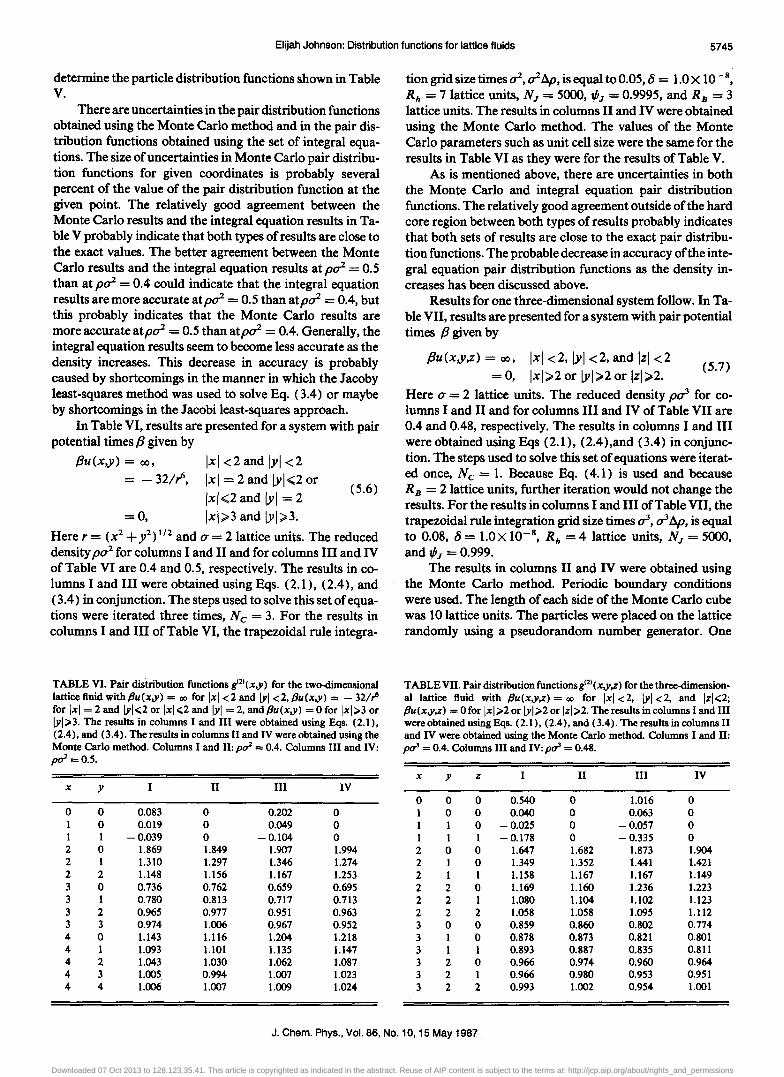
There are uncertainties in the pair distribution functions obtained using the Monte Carlo method and in the pair dis­tribution functions obtained using the set of integral equa­tions. The size of uncertainties in Monte Carlo pair distribu­tion functions for given coordinates is probably several percent of the value of the pair distribution function at the given point. The relatively good agreement between the Monte Carlo results and the integral equation results in Ta­ble V probably indicate that both types of results are close to the exact values. The better agreement between the Monte Carlo results and the integral equation results at pUZ = 0.5 than at pUZ = 0.4 could indicate that the integral equation results are more accurate at pUZ = 0.5 than at pUZ = 0.4, but this probably indicates that the Monte Carlo results are more accurate atpUZ = 0.5 than atpUZ = 0.4. Generally, the integral equation results seem to become less accurate as the density increases. This decrease in accuracy is probably caused by shortcomings in the manner in which the Jacoby least-squares method was used to solve Eq. (3.4) or maybe by shortcomings in the Jacobi least-squares approach.

In Table VI, results are presented for a system with pair potential times /3 given by

/3u(x,y) = 00,

= - 32/r'>, Ixl <2 and Jyl <2 Ixl = 2 and JyI<2 or

Ixl<2 and Iyl = 2 = 0, Ixl>3 and lyl>3.

(5.6)

Here r = (x2 + y2)1/2 and (J' = 2 lattice units. The reduced density pUZ for columns I and II and for columns III and IV of Table VI are 0.4 and 0.5, respectively. The results in co­lumns I and III were obtained using Eqs. (2.1), (2.4), and (3.4 ) in conjunction. The steps used to solve this set of equa­tions were iterated three times, N c = 3. For the results in columns I and III of Table VI, the trapezoidal rule integra-

TABLE VI. Pair distribution functions g'2)(X,y) for the two-dimensional lattice fluid with /1u(x,y) = 00 for Ixl <2 and Iyl <2, /1u(x,y) = - 32/,P for Ixl = 2 and lyl<2 or Ixl<2 and Iyl = 2, and/1u(x,y) = 0 for Ixl>3 or lyl>3. The results in columns I and III were obtained using Eqs. (2.1). (2.4). and (3.4). The results in columns II and IV were obtained using the Monte Carlo method. Columns I and II: per = 0.4. Columns III and IV: per =0.5.

x y II III IV

0 0 0.083 0 0.202 0 1 0 0.019 0 0.049 0 1 1 -0.039 0 - 0.104 0 2 0 1.869 1.849 1.907 1.994 2 1 1.310 1.297 1.346 1.274 2 2 1.148 1.156 1.167 1.253 3 0 0.736 0.762 0.659 0.695 3 1 0.780 0.813 0.717 0.713 3 2 0.965 0.977 0.951 0.963 3 3 0.974 1.006 0.967 0.952 4 0 1.143 1.116 1.204 1.218 4 1 1.093 1.101 1.135 1.147 4 2 1.043 1.030 1.062 1.087 4 3 1.005 0.994 1.007 1.023 4 4 1.006 1.007 1.009 1.024

tion grid size times UZ' UZ~, is equal to 0.05, 8 = LOX 10-8,

Rh = 7 lattice units, NJ = 5000, tPJ = 0.9995, and RB = 3 lattice units. The results in columns II and IV were obtained using the Monte Carlo method. The values of the Monte Carlo parameters such as unit cell size were the same for the results in Table VI as they were for the results of Table V.

As is mentioned above, there are uncertainties in both the Monte Carlo and integral equation pair distribution functions. The relatively good agreement outside of the hard core region between both types of results probably indicates that both sets of results are close to the exact pair distribu­tion functions. The probable decrease in accuracy of the inte­gral equation pair distribution functions as the density in­creases has been discussed above.

Results for one three-dimensional system follow. In Ta­ble VII, results are presented for a system with pair potential times /3 given by

/3u(x,y,z) = 00, Ixl <2, Jyl <2, and Izl <2 = 0, Ixl>2 or JyI>2 or Izl>2.

(5.7)

Here (J' = 2 lattice units. The reduced density per for co­lumns I and II and for columns III and IV of Table VII are 0.4 and 0.48, respectively. The results in columns I and III were obtained using Eqs (2.1), (2.4),and (3.4) in conjunc­tion. The steps used to solve this set of equations were iterat­ed once, N c = 1. Because Eq. (4.1) is used and because R B = 2 lattice units, further iteration would not change the results. For the results in columns I and III of Table VII, the trapezoidal rule integration grid size times er, er ~, is equal to 0.08, 8 = l.OX 10-8

, Rh = 4 lattice units, NJ = 5000, and tPJ = 0.999.

The results in columns II and IV were obtained using the Monte Carlo method. Periodic boundary conditions were used. The length of each side of the Monte Carlo cube was 10 lattice units. The particles were placed on the lattice randomly using a pseudorandom number generator. One

TABLE VII. Pair distribution functionsg'2)(x,y,z) for the three-dimension-al lattice fluid with /1u(x,y,z) = 00 for Ixl <2. IYI <2. and Izl<2; /1u(x,y,z) = o for Ixl>2 or lyl>2 or Izl>2. The results in columns I and III were obtained using Eqs. (2.1), (2.4), and (3.4). The results in columns II and IV were obtained using the Monte Carlo method. Columns I and II: pa3 = 0.4. Columns III and IV: pul = 0.48.

x y z II III IV

0 0 0 0.540 0 1.016 0 1 0 0 0.040 0 0.063 0 1 I 0 -0.025 0 -0.057 0 1 1 1 - 0.178 0 - 0.335 0 2 0 0 1.647 1.682 1.873 1.904 2 1 0 1.349 1.352 1.441 1.421 2 1 1 1.158 1.167 1.167 1.149 2 2 0 1.169 1.160 1.236 1.223 2 2 1 1.080 1.104 1.102 1.123 2 2 2 1.058 1.058 1.095 1.112 3 0 0 0.859 0.860 0.802 0.774 3 1 0 0.878 0.873 0.821 0.801 3 1 1 0.893 0.887 0.835 0.811 3 2 0 0.966 0.974 0.960 0.964 3 2 1 0.966 0.980 0.953 0.951 3 2 2 0.993 1.002 0.954 1.001

J. Chem. Phys., Vol. 86, No. 10, 15 May 1987

Downloaded 07 Oct 2013 to 128.123.35.41. This article is copyrighted as indicated in the abstract. Reuse of AIP content is subject to the terms at: http://jcp.aip.org/about/rights_and_permissions

5746 Elijah Johnson: Distribution functions for lattice fluids

thousand moves were made after the initial placement of the particles on the lattice. These initial moves were followed by 119 ()()() more moves. The last sets of moves were used to determine the particle distribution functions shown in Table VII.

As was the case for the two-dimensional systems, the agreement between the Monte Carlo and the integral equa­tion pair distribution functions is good. There are uncertain­ties in both the Monte Carlo and integral equations results.

VI. CONCLUSIONS

The technique for obtaining two- and three-particle dis­tribution functions used in this article is quite general. It is applicable to all classical systems which have a pairwise ad­ditive potential energy function. Some results of the tech­nique for several lattice fluids were presented. Exact results are available for some one-dimensional fluids, so the accura­cy of most of the results of the technique for the one-dimen­sional systems presented may be fully assessed. The results presented for these systems were accurate through about two decimal places. This accuracy was determined by com­paring with very accurate results which were determined by a technique presented in Ref. 1. Results from the integral equations for two- and three-dimensional systems were com­pared with corresponding Monte Carlo results.

The uncertainty in the particle distribution functions tends to increase as the density increases. A higher degree of numerical precision may be obtained in two ways. The first way is to make appropriate adjustments in the values of the numerical parameters Nc , Ap, R B , R h , tJ, NJ , and tPJ' The second way is to develop an improvement over the Jacobi least-squares procedure for solving the variational equation, Eq. (3.4). The development of an improved method for solv­ing the variational equation is perhaps the most important step for improving accuracy. It appears that the technique will give accurate results for any classical fluid with a pair­wise additive potential energy function when appropriate numerical techniques are used.

ACKNOWLEDGMENTS

The author is grateful to Dr. William R. Busing and to Dr. G. E. Wesenberg for their suggestions on how to solve the variational equation, Eq. (3.4). Dr. Busing suggested that an alternative to the Gaussian elimination procedure be sought. Dr. Wesenberg suggested the least-squares criterion approach.

APPENDIX

Basis functions for uniform and nonuniform one-di­mensionallattice gases were discussed in detail in Ref. 15. In Ref. 1, basis functions for uniform one-dimensional lattice fluids were presented. The basis sets used in this article con­tain more elements than the corresponding basis sets used in Ref. 1, so the relevant part of the Appendix of Ref. 1 is pre­sented here with appropriate changes.

Let r; be the position of particle i in one-dimensional

space. Let

and

LI = {r; Irj is the element of the set (r1,r2,r3) which is farthest to the left on the number line}, (AI)

L3 = {r; Irj is the element of the set (r1,r2,r3) which is farthest to the right on the number line}, (A2)

L2 = {rj Ir; ¥=L I' r;¥=L3, and rj is an element of (rl,r2,r3)}. (A3)

If IL3 -L21>ILI -L21, then let R2= IL I -L21 and R3 = IL 3 - L 21· If IL3 - L21 < ILl - L 21, then let R2 = IL 3 - L21 and R3 = ILl - L 21· Here IL; I denotes the absolute value of L;. Let Rs = R2 + R3 and let R6 = R3.

Let

P ~~ (Rs,R6) = tJy,(a,'y),R, tJy.(a,r),R.' (A4)

where tJjj is the Kronecker delta function, andYs(a,r) and Y6(a,r) map the pair (a,r) into integer values. The allowed values of Ys and Y6 are determined by the numerical limit chosen for Rs. The function Qar (Rs,R6) is defined by

Q~~(Rs,R6) =P~~(Rs,R6) +P~~(RB + 1,RB)' (A5)

It is assumed that E(Rs,R6) = 0 for Rs >RB. The basis functions Q ijO) are used in place of the functions denoted by Pij in Eq. (3.3).

In the case of interest here, the case when g(2)(x) = 0 when Ix I < u where u is defined by Eq. (5.1), it is necessary to exclude some of the basis functions in order to obtain a linearly independent basis set. These excluded functions are

( 1) Q ijO) (Rs,R6) for i = 1 through 4 when Rs - R6 < u andRs<u.

(2) Q ijO)(RS,R6) fori = 1 whenRs - R6 <uandRs>u.

Note that here the inequalities Rs < u and Rs>u replace the inequalities R6 < u and R6>U, respectively, in the corre­sponding conditions of Ref. 1.

Basis functions for uniform two- and three-dimensional lattice gases were discussed in detail in Ref. 5. The procedure for generalizing these basis sets to lattice fluids is analogous to this procedure for the one-dimensional case. To see this procedure, compare the discussion in the Appendices of Ref. 15 and of Ref. 1. The basis sets used in this article for two­and three-dimensional systems contain more elements than the corresponding basis sets used in Ref. 5. The procedure for including these extra basis functions is analogous to the procedure used above to include these basis functions for the one-dimensional case.

A particular procedure was used to perform the two summations in Eqs. (3.10) and (3.11) indicated by Sdrl2 and Sdr13 in order to reduce the computation time required to obtain these integrals. This procedure follows. Let

112 = X12 + RB - 1 + (Y12 + RB - 1) (2RB - 1)

+ (Z12 + RB - 1 )(2RB - 1)2. (A6)

When the rangeofx12'YI2' andz12 is (-RB + I,RB -1), each value of 112 corresponds to a different element of the set (XI2,y12,z12)' The maximum value of 112 is [(2RB - 1)3 - 1]. The lowest value is zero. For a given

J. Chem. Phys., Vol. 86, No.1 0, 15 May 1987

Downloaded 07 Oct 2013 to 128.123.35.41. This article is copyrighted as indicated in the abstract. Reuse of AIP content is subject to the terms at: http://jcp.aip.org/about/rights_and_permissions

Elijah Johnson: Distribution functions for lattice fluids 5747

value of 112, (XI2,y12,z12) is given by

and

Zl2 = - RB + 1 + 112/(2RB - 1 )2,

Yl2 = - RB + 1 + [/12 - (Z12 + RB - 1)

X(2RB _1)2]1(2RB -1),

(A7)

(AS)

X l2 = - RB + 1 + [/12 - (Z12 + RB - 1) (2RB - 1)2

- (Y12 +RB -1)(2Rb -1)]. (A9)

The quantity 113 is defined analogously to 112, Computation time is saved by using 112 and 113 as summation variables with the following restriction:

For two-dimensional cases, the following restrictions are also imposed:

and

YI2<X 12,

1 + YI2>O,

1 +x13>O,

1 + Y13>O.

For the three-dimensional case, the following extra restric­tions were imposed:

and

ZI2<;.Y12'

YI2<X I2,

1 +ZI2>O,

1 +XI3>O,

1 + Y13>O,

1 +Z13>O.

These restrictions prevented some redundancies in the sum­mations.

IE. Johnson, J. Chern. Phys. 82, 3779 (1985). 2E. Johnson, J. Chern. Phys. 72, 3010 (1980). 3J. A. Barker and D. Henderson, Rev. Mod. Phys. 48, 587 (1976). 4R. J. Baxter, J. Chern. Phys. 41, 553 (1964). sE. Johnson, J. Chern. Phys. 77, 3238 (1982). 6E. Johnson (unpublished). 7Z. W. Salsburg, R. W. Zwanzig, and J. G. Kirkwood, J. Chern. Phys. 21, 1098 (1953).

BL. L. Lee, J. Chern. Phys. 60,1197 (1974). 9J. K. Percus, in The Equilibrium Theory o/Classical Fluids, edited by H. L. Frisch and J. L. Lebowitz (W. A. Benjamin, New York, 1964), Eq. (5.12).

lOG. Stell, in Phase Transitions and Critical Phenomena, edited by C. Dornb and M. S. Green (Acadernic, New York, 1976), Vol. 5B.

llA. A. Broyles, J. Chern. Phys. 33, 456 (1960). 12A. M. Cohen, J. F. Cutts, R. Fielder, D. E. Jones, J. Ribbans, and E.

Stuart, Numerical Analysis (Wiley, New York, 1973), pp. 190-192. 13Reference 12, pp. 284-285. 14Reference 12, pp. 135-136. ISE. Johnson, J. Chern. Phys. 76, 2073 (1982). 16E. Johnson, G. R. Whittaker, and T. W. Breeden (unpublished).

J. Chern. Phys., Vol. 86, No. 10,15 May 1987

Downloaded 07 Oct 2013 to 128.123.35.41. This article is copyrighted as indicated in the abstract. Reuse of AIP content is subject to the terms at: http://jcp.aip.org/about/rights_and_permissions