Keyframe animation

Oldest keyframe animation

PraxinoscopeZoetropePhenakistiscope

1. Higher than 10 frames per second

2. A period of blackness between images

Two conditions to make a moving image in 19th century

2D animation

Highly skilled animators draw the keyframes

Less skilled (lower paid) animators draw the in-between frames

Difficult to create physically realistic animation

Time consuming process

3D animation

Animators specify important keyframes in 3D

Computers generates the in-between frames

Some dynamic motion can be done by computers (hair, clothes, etc)

Still time consuming; Pixar spent four years to produce Toy Story

From the making of toy story General pipeline

Story board

Keyframes

Inbetweens

Painting

Storyboards

The film in outline form

specify the key scenes

specify the camera moves and edits

specify character gross motion

Typically paper and pencil sketches on individual sheets taped on a wall

Story boarding from “a bug’s life”

http://www.pixar.com/featurefilms/ab!behind_pop4.html

The process of keyframing

Specify the keyframes

Specify the type of interpolation

linear, cubic, parametric curves

Specify the speed profile of the interpolation

constant velocity, ease-in-ease-out, etc

Computer generates the in-between frames

A keyframe

In 2D animation, a keyframe is usually a single image

In 3D animation, each keyframe is defined by a set of parameters

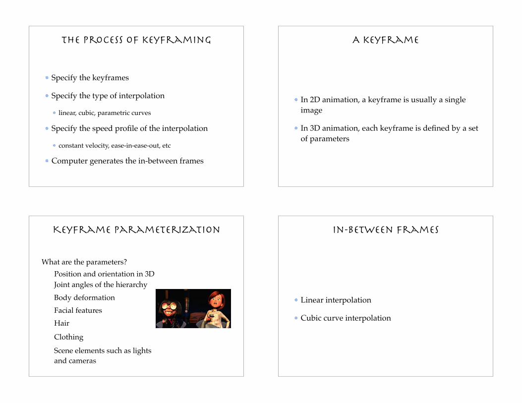
Keyframe parameterization

What are the parameters?

Position and orientation in 3D

Joint angles of the hierarchy

Body deformation

Facial features

Hair

Clothing

Scene elements such as lights

and cameras

in-between frames

Linear interpolation

Cubic curve interpolation

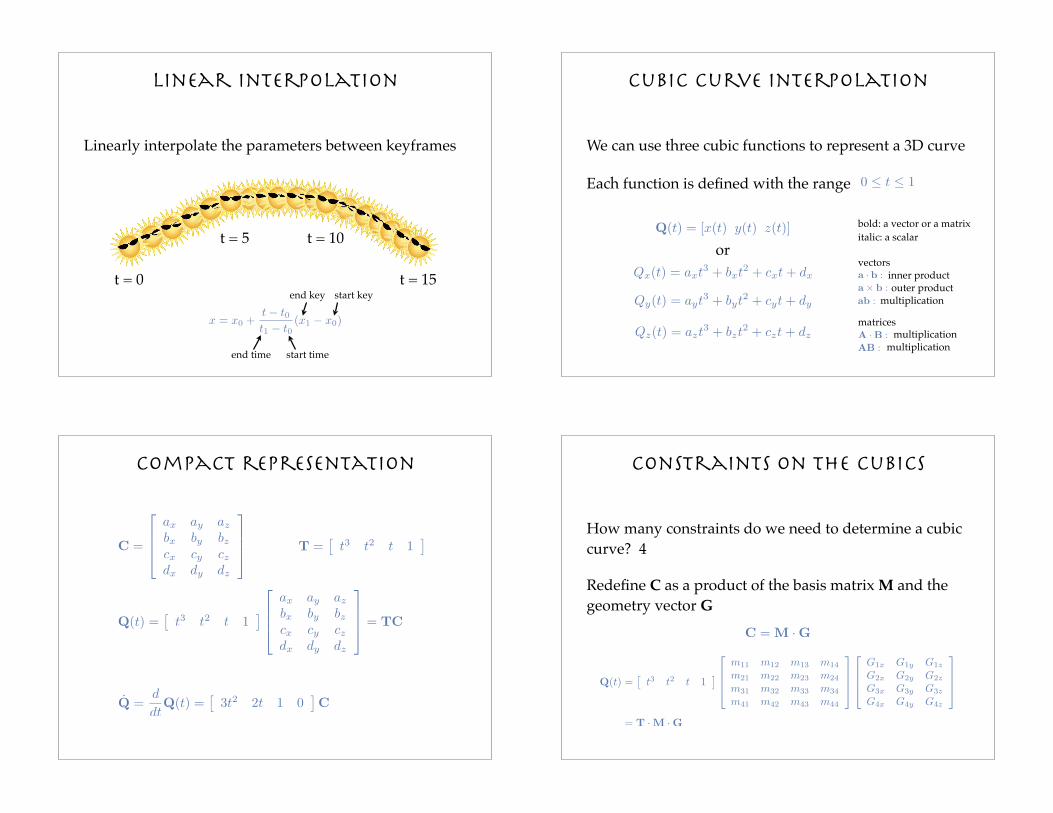
Linear interpolation

Linearly interpolate the parameters between keyframes

x = x0 +t ! t0

t1 ! t0(x1 ! x0)

end key start key

end time start time

t = 0

t = 5 t = 10

t = 15

Cubic curve interpolation

Qx(t) = axt3 + bxt2 + cxt + dx

Qy(t) = ayt3 + byt2 + cyt + dy

Qz(t) = azt3 + bzt

2 + czt + dz

Q(t) = [x(t) y(t) z(t)]

or

We can use three cubic functions to represent a 3D curve

0 ! t ! 1Each function is defined with the range

bold: a vector or a matrix

italic: a scalar

a · b : inner producta ! b : outer productab : multiplication

vectors

matricesA · B :

AB :

multiplicationmultiplication

Compact representation

C =

!

"

"

#

ax ay az

bx by bz

cx cy cz

dx dy dz

$

%

%

&

T =!

t3

t2

t 1"

Q(t) =!

t3 t2 t 1"

#

$

$

%

ax ay az

bx by bz

cx cy cz

dx dy dz

&

'

'

(

= TC

d

dtQ(t) =

!

3t2 2t 1 0"

CQ̇ =

Constraints on the cubics

Q(t) =!

t3 t2 t 1"

#

$

$

%

m11 m12 m13 m14

m21 m22 m23 m24

m31 m32 m33 m34

m41 m42 m43 m44

&

'

'

(

#

$

$

%

G1x G1y G1z

G2x G2y G2z

G3x G3y G3z

G4x G4y G4z

&

'

'

(

= T · M · G

How many constraints do we need to determine a cubic

curve?

C = M · G

Redefine C as a product of the basis matrix M and the

geometry vector G

4

Hermite curves

A Hermite curve is determined by

1. endpoints P1 and P4 P1

P4

2. tangent vectors R1 and R4 at the endpoints

R4

R1

Gh =

!

"

"

#

P1x P1y P1z

P4x P4y P4z

R1x R1y R1z

R4x R4y R4z

$

%

%

&

Use these elements to construct the geometry vector

Hermite basis matrix

Given desired constraints:

Q(0) =!

0 0 0 1"

· Mh · Gh = P1

Q(1) =!

1 1 1 1"

· Mh · Gh = P4

1. endpoints meet P1 and P4

Q!(1) =!

3 2 1 0"

· Mh · Gh = R4

2. tangent vectors meet R1 and R4

Q!(0) =!

0 0 1 0"

· Mh · Gh = R1

Hermite basis matrix

We can solve for basis matrix Mh

!

"

"

#

P1

P4

R1

R4

$

%

%

&

= Gh =

!

"

"

#

0 0 0 1

1 1 1 1

0 0 1 0

3 2 1 0

$

%

%

&

· Mh · Gh

Mh =

!

"

"

#

0 0 0 1

1 1 1 1

0 0 1 0

3 2 1 0

$

%

%

&

!1

=

!

"

"

#

2 !2 1 1

!3 3 !2 !1

0 0 1 0

1 0 0 0

$

%

%

&

Hermite Blending functions

Let’s define B as a product of T and M

Bh(t) =!

t3

t2

t 1"

#

$

$

%

2 !2 1 1!3 3 !2 !10 0 1 01 0 0 0

&

'

'

(

Bh(t) indicates the weight of each element in Gh

Q(t) = Bh(t) ·

!

"

"

#

P1

P4

R1

R4

$

%

%

&

t

P1 P4

R4

R1

Bh(t)

Bézier curves

Indirectly specify tangent vectors by specifying two

intermediate points

Gb =

!

"

"

#

P1

P2

P3

P4

$

%

%

&

R4 = 3(P4 ! P3)

P3

P4

R4

R1 = 3(P2 ! P1)

P1

P2

R1

Bézier basis matrix

Establish the relation between Hermite and Bezier

geometry vectors

Gh =

!

"

"

#

P1

P4

R1

R4

$

%

%

&

=

!

"

"

#

1 0 0 0

0 0 0 1

!3 3 0 0

0 0 !3 3

$

%

%

&

!

"

"

#

P1

P2

P3

P4

$

%

%

&

= Mhb · Gb

Bézier basis matrix

Q(t) = T · Mh · Gh = T · Mh · (Mhb · Gb)

= T · (Mh · Mhb) · Gb = T · Mb · Gb

Mb = MhMhb =

!

"

"

#

!1 3 !3 1

3 !6 3 0

!3 3 0 0

1 0 0 0

$

%

%

&

http://www.cs.unc.edu/~mantler/research/bezier/index.html

Bézier blending functions

Bb(t) =!

t3

t2

t 1"

#

$

$

%

!1 3 !3 13 !6 3 0!3 3 0 01 0 0 0

&

'

'

(

Bezier blending functions are also called Bernstein

polynomials

Q(t) = Bb(t) ·

!

"

"

#

P1

P2

P3

P4

$

%

%

&

t

Bb(t)

P1

P2 P3

P4

Complex curves

What if we want to model a curve that passes through

these points?

Problem with higher order polynomials:

Wiggly curves

No local control

Splines

A piecewise polynomial function that has locally very simple form, yet be globally flexible and smooth

There are three nice properties of splines we’d like to have

Continuity

Local control

Interpolation

Continuity

Cubic curves are continuous and differentiable

We only need to worry about the derivatives at the endpoints when two curves meet

Continuity

C0: points coincide, velocities don’t

C1: points and velocities coincide

What’s C2? points, velocities and accelerations coincide

Local control

Bezier and Hermite curves don’t have local control; moving a single control point affects the whole curve

We’d like to have each control point on the spline only affect some well-defined neighborhood around that point

Interpolation

Bezier curves do not necessarily pass through all the control points

We’d like to have a spline interpolating the control points so that the spline always passes through every control points

B-splines

We can join multiple Bezier curves to create B-splines

Ensure C2 continuity when two curves meet

Continuity in B-splines

Qv(1) = Qw(0)

Q!

v(1) = Q!

w(0)

Q!!

v(1) = Q!!

w(0)

V3 = W0

V3 ! V2 = W1 ! W0

V1 ! 2V2 + V3 = W0 ! 2W1 + W2

W2 = V1 + 4V3 ! 4V2

Suppose we want to join two Bezier curves (V0, V1, V2, V3)

and (W0, W1, W2, W3) so that C2 continuity is met at the joint

V0

V1V2

V3 W0

W1 W2

W3

B1

V0

V1 V2

V3 = W0

W0 = V3

W2

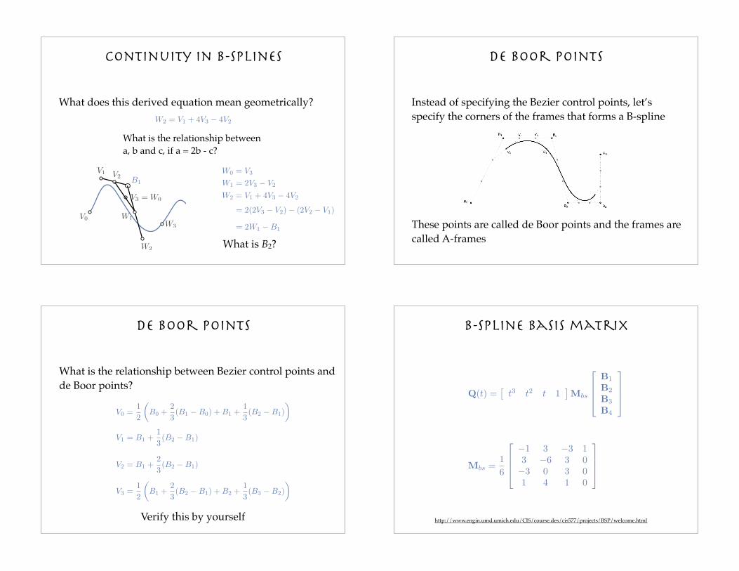
Continuity in B-splines

What does this derived equation mean geometrically?

W2 = V1 + 4V3 ! 4V2

= 2(2V3 ! V2) ! (2V2 ! V1)

= 2W1 ! B1

W1

W3

What is the relationship between a, b and c, if a = 2b - c?

W2 = V1 + 4V3 ! 4V2

What is B2?

W1 = 2V3 ! V2

de Boor points

These points are called de Boor points and the frames are

called A-frames

Instead of specifying the Bezier control points, let’s

specify the corners of the frames that forms a B-spline

de boor points

What is the relationship between Bezier control points and

de Boor points?

Verify this by yourself

V1 = B1 +1

3(B2 ! B1)

V0 =1

2

!

B0 +2

3(B1 ! B0) + B1 +

1

3(B2 ! B1)

"

V2 = B1 +2

3(B2 ! B1)

V3 =1

2

!

B1 +2

3(B2 ! B1) + B2 +

1

3(B3 ! B2)

"

B-spline basis matrix

Mbs =1

6

!

"

"

#

!1 3 !3 1

3 !6 3 0

!3 0 3 0

1 4 1 0

$

%

%

&

Q(t) =!

t3

t2

t 1"

Mbs

#

$

$

%

B1

B2

B3

B4

&

'

'

(

http://www.engin.umd.umich.edu/CIS/course.des/cis577/projects/BSP/welcome.html

B-Spline properties

C2 continuity?

Local control?

Interpolation?

B-Spline properties

C2 continuity?

Local control?

Interpolation?

Catmull-Rom splines

If we are willing to sacrifice C2 continuity, we can get interpolation and local control

If we set each derivative to be a constant multiple of the vector between the previous and the next controls, we get a Catmull-Rom spline

Catmull-Rom splines

Dn = Cn ! Cn!1

.

.

.

C0

C1

C2

C3

D0 = C1 ! C0

D0

D1 =1

2(C2 ! C0) D1

D2 =1

2(C3 ! C1) D2

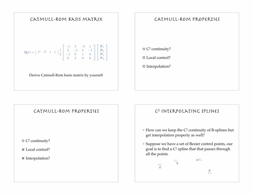
Catmull-Rom Basis matrix

Derive Catmull-Rom basis matrix by yourself

Q(t) =!

t3

t2

t 1" 1

2

#

$

$

%

!1 3 !3 12 !5 4 !1!1 0 1 00 2 0 0

&

'

'

(

#

$

$

%

P1

P2

P3

P4

&

'

'

(

CATmull-Rom properties

C2 continuity?

Local control?

Interpolation?

CATmull-Rom properties

C2 continuity?

Local control?

Interpolation?

C2 interpolating splines

How can we keep the C2 continuity of B-splines but get interpolation property as well?

Suppose we have a set of Bezier control points, our goal is to find a C2 spline that that passes through all the points

C0

C1C2

C3

C2 interpolating splines

C0

C1C2

C3D0

D1

D2

D3

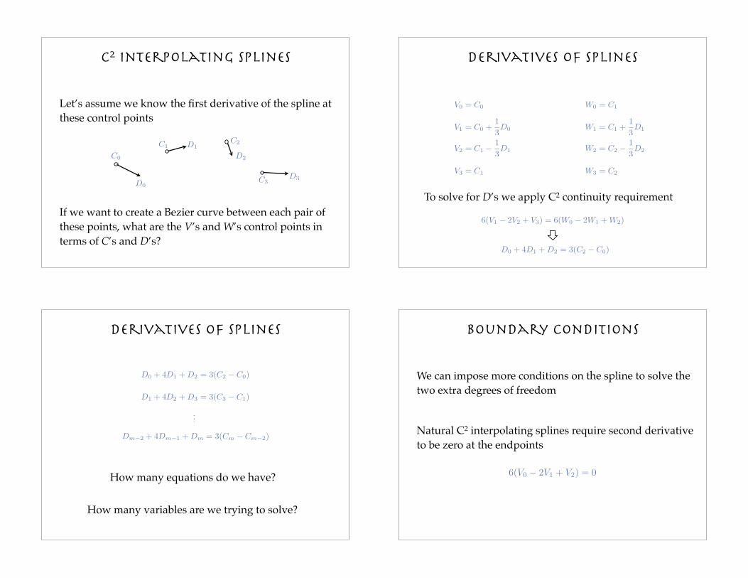
Let’s assume we know the first derivative of the spline at

these control points

If we want to create a Bezier curve between each pair of

these points, what are the V’s and W’s control points in

terms of C’s and D’s?

Derivatives of splines

V0 = C0

V1 = C0 +1

3D0

V3 = C1

W0 = C1

W1 = C1 +1

3D1

W3 = C2

V2 = C1 !

1

3D1 W2 = C2 !

1

3D2

6(V1 ! 2V2 + V3) = 6(W0 ! 2W1 + W2)

To solve for D’s we apply C2 continuity requirement

D0 + 4D1 + D2 = 3(C2 ! C0)

Derivatives of splines

D0 + 4D1 + D2 = 3(C2 ! C0)

D1 + 4D2 + D3 = 3(C3 ! C1)

Dm!2 + 4Dm!1 + Dm = 3(Cm ! Cm!2)

.

.

.

How many equations do we have?

How many variables are we trying to solve?

Boundary conditions

We can impose more conditions on the spline to solve the

two extra degrees of freedom

Natural C2 interpolating splines require second derivative

to be zero at the endpoints

6(V0 ! 2V1 + V2) = 0

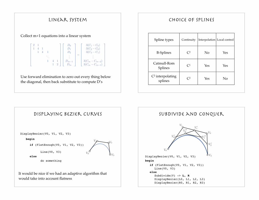
Linear system

Collect m+1 equations into a linear system

!

"

"

"

"

"

"

"

#

2 11 4 1

1 4 1. . .1 4 1

1 2

$

%

%

%

%

%

%

%

&

!

"

"

"

"

"

"

"

#

D0

D1

D2

...Dm!1

Dm

$

%

%

%

%

%

%

%

&

=

!

"

"

"

"

"

"

"

#

3(C1 ! C0)3(C2 ! C0)3(C3 ! C1)

...3(Cm ! Cm!2)3(Cm ! Cm!1)

$

%

%

%

%

%

%

%

&

Use forward elimination to zero out every thing below

the diagonal, then back substitute to compute D’s

Choice of splines

Spline types Continuity Interpolation Local control

B-Splines C2 No Yes

Catmull-Rom Splines

C1 Yes Yes

C2 interpolating splines

C2 Yes No

Displaying Bezier curves

DisplayBezier(V0, V1, V2, V3)

begin

if (FlatEnough(V0, V1, V2, V3))

Line(V0, V3)

else

do something

It would be nice if we had an adaptive algorithm that

would take into account flatness

V0

V1V2

V3

V0

V1

V2

V3

Subdivide and Conquer

V!

0

V!

1

V!

2

V!!

0

V!!

1

DisplayBezier(V0, V1, V2, V3)

begin

if (FlatEnough(V0, V1, V2, V3))

! Line(V0, V3)

else

! Subdivide(V) -> L, R

! DisplayBezier(L0, L1, L2, L3)

! DisplayBezier(R0, R1, R2, R3)

Flatness Test

V0

V1

V2

V3

Compare total length of control polygon to length of line

connecting endpoints:

|V0 ! V1| + |V1 ! V2| + |V2 ! V3|

|V0 ! V3|< 1 + !

Endpoints of B-splines

We can see that B-splines don’t interpolate the de Boor points

It would be nice if we could at least control the endpoints of the splines explicitly

There’s a trick to make the spline begin and end at the de Boor points by repeating them

Curves in the animation

Each animation parameter is determined by a 2D curve

Q(u) = (x(u), y(u))

Treat this curve as!(u) = y(u)

t(u) = x(u)

!

!(t)

where is a variable you want to animate. We can think

of the results as a function:

!(t)Apply constraints to make sure that actually is a

function

Wrapping the curves

Wrapping is an important feature that makes the animation restart smoothly when looping back to the beginning

Create “phantom” control points before and after the first and the last control points

C!1

Cn+1C0

C1

C2

Cn

t

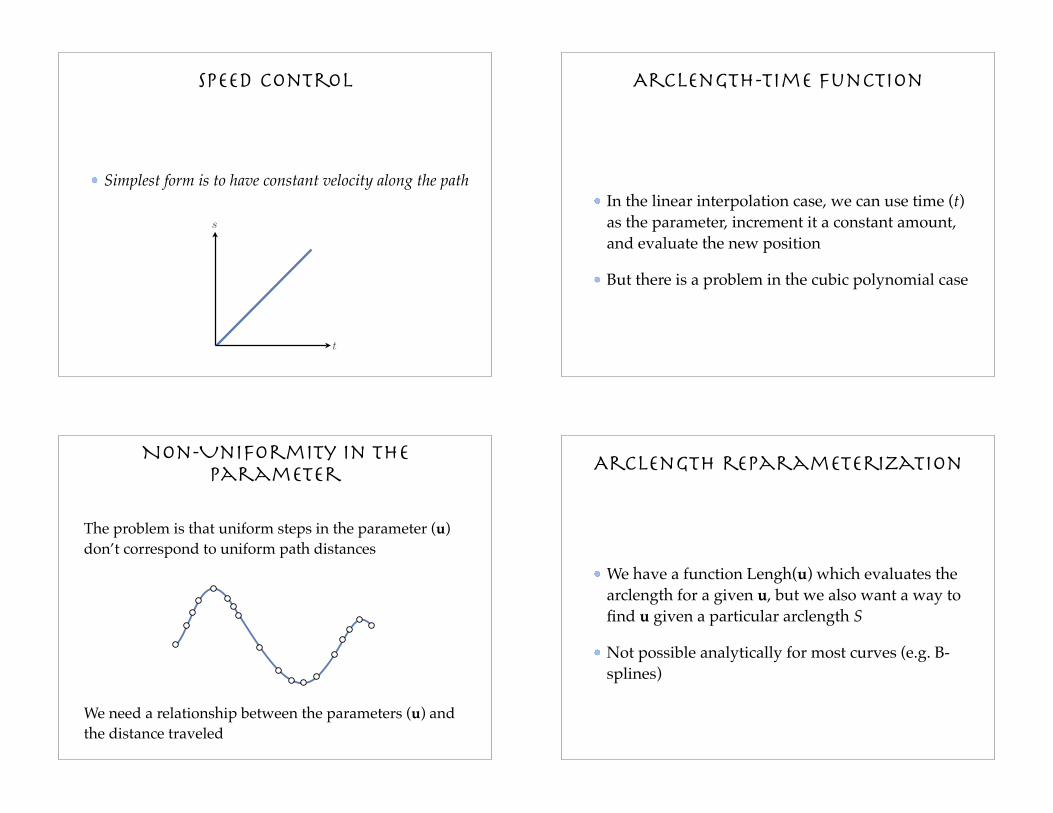
Speed control

Simplest form is to have constant velocity along the path

t

s

Arclength-Time function

In the linear interpolation case, we can use time (t) as the parameter, increment it a constant amount, and evaluate the new position

But there is a problem in the cubic polynomial case

Non-Uniformity in the parameter

The problem is that uniform steps in the parameter (u)

don’t correspond to uniform path distances

We need a relationship between the parameters (u) and

the distance traveled

Arclength reparameterization

We have a function Lengh(u) which evaluates the arclength for a given u, but we also want a way to find u given a particular arclength S

Not possible analytically for most curves (e.g. B-splines)

Finite Differences

Sample the curve at small intervals of the parameter and determine the distance between samples

Use theses distances to build a table of arclength for this particular curve

index parametric value arclength01234

0.000.050.100.150.20

0.000

0.320

0.080

0.2300.150

Finite differences

If we want to know S at a particular value of the parameter u = 0.73, spacing of the table is 0.05

Find the entry in the table closest to this u

Or take the u before and after it and interpolate linearly

Similarly, we can find u for a given S

Speed control recipe

Given a time t, lookup the corresponding arclength S in the speed curve

For S, look up the corresponding value of u in the reparameterization table

Evaluate the curve at u to obtain the correct interpolated position for the animated object for the given time t

Ease-in Ease-out curve

Assume that the motion slows down at the beginning and end of the motion curve

t

s

Do you know this?

Why does a movie run at 24 frames per second while a TV runs at 30 frames per second?

Open questions

What should the key values be?

When should the key values occur?

Are there better ways to specify key values?

What kind of bad things can occur from interpolation? How do we prevent them?

Invalid configurations (pass through walls)

Unnatural motions (painful twists)

What’s next?

What about rotations?

Can we interpolate rotations using the these same techniques?