1 Two-Dimensional Computational Fluid Dynamics and Conduction Simulations of Heat Transfer in Window Frames with Internal Cavities - Part 1: Cavities Only Arild Gustavsen, Christian Kohler, Dariush Arasteh and Dragan Curcija ABSTRACT Accurately analyzing heat transfer in window frame cavities is essential for developing and characterizing the performance of highly insulating window products. Window frame thermal performance strongly influences overall product thermal performance because framing materials generally perform much more poorly than glazing materials. This paper uses Computational Fluid Dynamics (CFD) modeling to assess the accuracy of the simplified frame cavity conduction/convection models presented in ISO 15099 and used in software for rating and labeling window products. (We do not address radiation heat-transfer effects.) We examine three representative complex cavity cross-section profiles with varying dimensions and aspect ratios. Our results support the ISO 15099 rule that complex cavities with small throats should be subdivided; however, our data suggest that cavities with throats smaller than seven millimeters (mm) should be subdivided, in contrast to the ISO 15099 rule, which places the break point at five mm. The agreement between CFD modeling results and the results of the simplified models is moderate. The differences in results may be a result of the underlying ISO correlations being based on studies where cavity height/length (H/L) aspect ratios were smaller than 0.5 and greater than five (with linear interpolation assumed in between). The results presented here are for horizontal frame members because convection in vertical jambs involves very different aspect
Transcript
1
Two-Dimensional Computational Fluid Dynamics and Conduction Simulations of Heat Transfer in Window Frames
with Internal Cavities - Part 1: Cavities Only
Arild Gustavsen, Christian Kohler, Dariush Arasteh and Dragan Curcija
ABSTRACT
Accurately analyzing heat transfer in window frame cavities is essential for developing
and characterizing the performance of highly insulating window products. Window frame
thermal performance strongly influences overall product thermal performance because framing
materials generally perform much more poorly than glazing materials. This paper uses
Computational Fluid Dynamics (CFD) modeling to assess the accuracy of the simplified frame
cavity conduction/convection models presented in ISO 15099 and used in software for rating and
labeling window products. (We do not address radiation heat-transfer effects.) We examine three
representative complex cavity cross-section profiles with varying dimensions and aspect ratios.
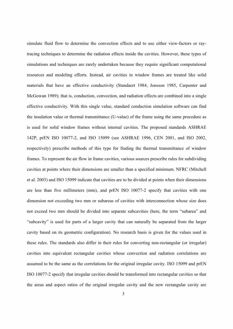
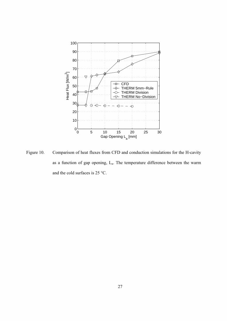
Our results support the ISO 15099 rule that complex cavities with small throats should be
subdivided; however, our data suggest that cavities with throats smaller than seven millimeters
(mm) should be subdivided, in contrast to the ISO 15099 rule, which places the break point at
five mm. The agreement between CFD modeling results and the results of the simplified models
is moderate. The differences in results may be a result of the underlying ISO correlations being
based on studies where cavity height/length (H/L) aspect ratios were smaller than 0.5 and
greater than five (with linear interpolation assumed in between). The results presented here are
for horizontal frame members because convection in vertical jambs involves very different aspect
2
ratios that require three-dimensional CFD simulations. Ongoing work focuses on quantifying the
exact effect on window thermal performance indicators of using the ISO 15099 approximations in
typical real window frames.
INTRODUCTION
The frame is an important part of a fenestration product. In a window with a total area of
1.2 × 1.2 m2 and a frame with a width of 10 cm, the frame occupies 30 percent of the window’s
total area. If the total area of the window is increased to 2.0 × 2.0 m2, the same frame occupies 19
percent of the total area. When rating a fenestration product, engineers area-weight the thermal
performance of the different parts of the product to determine a single number that describes the
entire product. Thus, to be able to accurately calculate a product's thermal performance, engineers
need models that accurately describe the thermal performance of each part of the product or
accurate measurements of actual thermal performance. Because actual measurement is expensive,
use of accurate models is preferable.
A significant body of research has focused on heat-transfer effects in glazing cavities. The
primary goal of that work has been to develop accurate correlations for natural convection effects
inside multiple-pane windows (Batchelor 1954, Eckert and Carlson 1961, Hollands et al. 1976,
Raithby et al. 1977, Berkovsky and Polevikov 1977, ElSherbiny et al. 1982, Shewen et al. 1996,
Wright 1996, and Zhao 1998). Less research has been conducted on heat transfer in window
frames that have internal cavities. This is an important issue for high-performance window
frames because cavities are a primary area where frame heat transfer can be minimized (the
thermal conductivity of solid framing materials is another key area). In window frames with
internal cavities, the heat-transfer process involves a combination of conduction, convection, and
radiation. To fully describe heat transfer through these window frames, it would be necessary to
3
simulate fluid flow to determine the convection effects and to use either view-factors or ray-
tracing techniques to determine the radiation effects inside the cavities. However, these types of
simulations and techniques are rarely undertaken because they require significant computational
resources and modeling efforts. Instead, air cavities in window frames are treated like solid
materials that have an effective conductivity (Standaert 1984, Jonsson 1985, Carpenter and
McGowan 1989); that is, conduction, convection, and radiation effects are combined into a single
effective conductivity. With this single value, standard conduction simulation software can find
the insulation value or thermal transmittance (U-value) of the frame using the same procedure as
is used for solid window frames without internal cavities. The proposed standards ASHRAE
142P, prEN ISO 10077-2, and ISO 15099 (see ASHRAE 1996, CEN 2001, and ISO 2002,
respectively) prescribe methods of this type for finding the thermal transmittance of window
frames. To represent the air flow in frame cavities, various sources prescribe rules for subdividing
cavities at points where their dimensions are smaller than a specified minimum. NFRC (Mitchell
et al. 2003) and ISO 15099 indicate that cavities are to be divided at points when their dimensions
are less than five millimeters (mm), and prEN ISO 10077-2 specify that cavities with one
dimension not exceeding two mm or subareas of cavities with interconnection whose size does
not exceed two mm should be divided into separate subcavities (here, the term “subarea” and
“subcavity” is used for parts of a larger cavity that can naturally be separated from the larger
cavity based on its geometric configuration). No research basis is given for the values used in
these rules. The standards also differ in their rules for converting non-rectangular (or irregular)
cavities into equivalent rectangular cavities whose convection and radiation correlations are
assumed to be the same as the correlations for the original irregular cavity. ISO 15099 and prEN
ISO 10077-2 specify that irregular cavities should be transformed into rectangular cavities so that
the areas and aspect ratios of the original irregular cavity and the new rectangular cavity are
4
equal. ASHRAE 142P specifies that irregular cavities should be transformed into rectangular
cavities using a bounding rectangle. The aspect ratios and the total heights and widths of the
original irregular cavity and the new rectangular cavity should be equal. (The total heights and
widths will most likely not be equal under ISO 15099 and prEN ISO 10077-2.)
In this paper, we focus on convective heat transfer in frame cavities; problems related to
dividing cavities and transforming irregular cavities into rectangular cavities are addressed.
Computational fluid dynamics (CFD) and conduction simulations were conducted for this study.
In the conduction simulations, an effective conductivity was used to account for both conduction
and convection in frame cavities. In a companion paper the U-values of complete window frames
with internal cavities are studied.
GEOMETRIES STUDIED
The air cavities studied are shown in Figure 1. The particular cavities were chosen to
represent air cavities that can be found in real window frames. The cavities are identified as H-
cavity, L-cavity and C-cavity (left to right in Figure 1). H-cavity is square with two solid fins
protruding into it. Measurements and temperature differences simulated for the cavities are
shown in Tables 1 to 3. Because the cavities are simulated in two dimensions, the results are valid
for horizontal frame members. CFD results that are valid for jamb sections require simulations in
three dimensions.
Table 1. Cavity measures and temperatures for the H-cavity.