Hindawi Publishing Corporation Mathematical Problems in Engineering Volume 2012, Article ID 581493, 26 pages doi:10.1155/2012/581493 Research Article Two-Dimensional Fracture Mechanics Analysis Using a Single-Domain Boundary Element Method Chien-Chung Ke, 1 Cheng-Lung Kuo, 2 Shih-Meng Hsu, 1 Shang-Chia Liu, 2 and Chao-Shi Chen 3 1 Geotechnical Engineering Research Center, Sinotech Engineering Consultants, Inc., Taipei 110, Taiwan 2 Department of Business Administration, Fu Jen Catholic University, New Taipei City 242, Taiwan 3 Department of Resources Engineering, National Cheng Kung University, Tainan 701, Taiwan Correspondence should be addressed to Chien-Chung Ke, [email protected]Received 13 March 2012; Accepted 21 March 2012 Academic Editor: Kue-Hong Chen Copyright q 2012 Chien-Chung Ke et al. This is an open access article distributed under the Creative Commons Attribution License, which permits unrestricted use, distribution, and reproduction in any medium, provided the original work is properly cited. This work calculates the stress intensity factors SIFsat the crack tips, predicts the crack initiation angles, and simulates the crack propagation path in the two-dimensional cracked anisotropic materials using the single-domain boundary element method BEMcombined with maximum circumferential stress criterion. The BEM formulation, based on the relative displacements of the crack tip, is used to determine the mixed-mode SIFs and simulate the crack propagation behavior. Numerical examples of the application of the formulation for different crack inclination angles, crack lengths, degree of material anisotropy, and crack types are presented. Furthermore, the propagation path in Cracked Straight Through Brazilian Disc CSTBDspecimen is numerically predicted and the results of numerical and experimental data compared with the actual laboratory observations. Good agreement is found between the two approaches. The proposed BEM formulation is therefore suitable to simulate the process of crack propagation. Additionally, the anisotropic rock slope failure initiated by the tensile crack can also be analyzed by the proposed crack propagation simulation technique. 1. Introduction Fracture mechanics theory has been developed to solve many geotechnical engineering problems, such as blasting, hydraulic fracturing, and slope stability. In two-dimensional fracture mechanics problems, SIFs are important parameters in analysis of cracked materials. The singularity of stresses near the crack tip is the challenge to numerical modelling methods, even to the BEM. Because the coincidence of the crack surfaces gives rise to a singular system of algebraic equations, the solution of cracked problem cannot be obtained with the direct
Transcript
Hindawi Publishing CorporationMathematical Problems in EngineeringVolume 2012, Article ID 581493, 26 pagesdoi:10.1155/2012/581493
Research ArticleTwo-Dimensional Fracture Mechanics AnalysisUsing a Single-Domain Boundary Element Method
Chien-Chung Ke,1 Cheng-Lung Kuo,2 Shih-Meng Hsu,1Shang-Chia Liu,2 and Chao-Shi Chen3
1 Geotechnical Engineering Research Center, Sinotech Engineering Consultants, Inc.,Taipei 110, Taiwan
2 Department of Business Administration, Fu Jen Catholic University, New Taipei City 242, Taiwan3 Department of Resources Engineering, National Cheng Kung University, Tainan 701, Taiwan
Correspondence should be addressed to Chien-Chung Ke, [email protected]
Received 13 March 2012; Accepted 21 March 2012
Academic Editor: Kue-Hong Chen
Copyright q 2012 Chien-Chung Ke et al. This is an open access article distributed under theCreative Commons Attribution License, which permits unrestricted use, distribution, andreproduction in any medium, provided the original work is properly cited.
This work calculates the stress intensity factors (SIFs) at the crack tips, predicts the crack initiationangles, and simulates the crack propagation path in the two-dimensional cracked anisotropicmaterials using the single-domain boundary element method (BEM) combined with maximumcircumferential stress criterion. The BEM formulation, based on the relative displacements of thecrack tip, is used to determine the mixed-mode SIFs and simulate the crack propagation behavior.Numerical examples of the application of the formulation for different crack inclination angles,crack lengths, degree of material anisotropy, and crack types are presented. Furthermore, thepropagation path in Cracked Straight Through Brazilian Disc (CSTBD) specimen is numericallypredicted and the results of numerical and experimental data compared with the actual laboratoryobservations. Good agreement is found between the two approaches. The proposed BEMformulation is therefore suitable to simulate the process of crack propagation. Additionally, theanisotropic rock slope failure initiated by the tensile crack can also be analyzed by the proposedcrack propagation simulation technique.
1. Introduction
Fracture mechanics theory has been developed to solve many geotechnical engineeringproblems, such as blasting, hydraulic fracturing, and slope stability. In two-dimensionalfracture mechanics problems, SIFs are important parameters in analysis of cracked materials.The singularity of stresses near the crack tip is the challenge to numerical modelling methods,even to the BEM. Because the coincidence of the crack surfaces gives rise to a singular systemof algebraic equations, the solution of cracked problem cannot be obtained with the direct
2 Mathematical Problems in Engineering
formulation of the BEM. Several special methods within the scope of the BEM have beensuggested for handling stress singularities, such as the Green’s function method [1], thesubregional method [2–4], and the displacement discontinuity method (DDM) [5–7].
The Green’s function method overcomes the crack modelling problem withoutconsidering any source point along the crack boundaries. This method has the advantageof avoiding crack surface modelling and gives excellent accuracy; it is, however, restricted tovery simple crack geometries for which analytical Green’s function is available. The sub-regional method has the advantage of modelling cracks with any geometric shape. Themethod has the disadvantage of introducing the artificial boundaries of the original regioninto several subregions, thus resulting in a large system of equations. In crack propagationanalysis, these artificial boundaries must be repeatedly introduced for each increment ofthe crack extension. Therefore, this method cannot be easily implemented as an automaticprocedure in an incremental analysis of crack extension problems. The DDM overcomesthe crack modelling by replacing each pair of coincident source points on crack boundariesby a single source point [8]. Instead of using the Green’s stresses and displacements frompoint forces, the DDM uses Green’s functions corresponding to point dislocations, that is,displacement discontinuities. This method is quite suitable for crack problems in infinitedomains where there is no crack boundary. However, it alone may not be efficient for finitedomain problems since the kernel functions in the DDM involve singularities with orderhigher than those in the traditional displacement BEM. Hence, this method is not suitable forproblems involving finite domains.
With the advances in single-domain BEM in recent decades, it involves two setsof boundary integral equations for the study of cracked media [9–21]. The single-domainanalysis can eliminate remeshing problems, which are typical of the FEM and the subregionalBEM. The single-domain BEM has received considerable attention and has been found to bea proper method for simulating crack propagation processes.
The single-domain BEM formulation can be achieved by applying the displacementintegral equation to the no-crack boundary only, and the traction integral equation on oneside of the crack surface only. Since only one side of the crack surface is collocated, one needsto choose either the relative crack opening displacement (COD). This BEM formulation canbe applied to the general fracture mechanics analysis in anisotropic media while keeping thesingle-domain merit.
In this study, the BEM formulation combined with the maximum circumferentialstress criterion is adopted to predict the crack initiation angles and to simulate thecrack propagation paths. Crack propagation in an anisotropic homogeneous plate undermixed-mode I-II loading is simulated by an incremental crack growth with a piece-wiselinear discretization. A new computer program, which can automatically generate a newmesh required for analyzing the changing boundary configuration sequentially, has beendeveloped to simulate the fracture propagation process. To demonstrate the proposed BEMprocedure for predicting crack propagation in anisotropic materials, the propagation path ina CSTBD is numerically predicted and compared with the actual laboratory observations.
A geotechnical engineering problem, slope stability, was analyzed here by theproposed crack propagation simulation technique. Slope stability analysis in the past reliedheavily on the use of the limit equilibrium method. An analysis is often carried out byfirst assuming a failure mode, then using an extensive search to determine the location ofcritical failure surface. From the type of analysis, estimates of the normal and shear stressdistribution on the failure surface and a factor of safety are obtained. This type of study hasproved very effective for most engineering applications. However, numerical models, such
Mathematical Problems in Engineering 3
as continuum models and discontinuum models, tend to be general purpose in nature; thatis, they are capable of solving a wide variety of problems. While it is often desirable to havea general-purpose tool available, it requires that each problem be constructed individually.The zones must be arranged by the user to fit the limits of geomechanical units and/or theslope geometry. Hence, numerical models often require more time to set up and run thanspecial-purpose tools such as limit equilibrium method.
In the past, the two most popular techniques in continuum mechanics, namely, finiteelement method (FEM) and finite difference method (FDM), are used in the analysis ofthe slope stability problems. Early numerical analyses of rock slopes were predominantlyundertaken using continuum finite element codes. Kalkani and Piteau (1976) [22], forexample, used this method to analyze toppling of rock slopes at Hells Gate in BritishColumbia, Canada, and Krahn and Morgenstern (1976) [23] undertook preliminary finiteelement modeling of the Frank Slide in Albetra, Canada. More recently, Stacey et al. in 2003[24] used finite element analysis in an innovative analysis of extensile strain distributionsassociated with deep open pit mines. The use of finite difference codes has predominantlyinvolved the use of the FLAC 2D and 3D codes [25]. Coggan et al. (2000) [26] demonstratedthe use of both 2D and 3D finite difference analyses in the back analysis of highly kaolinisedchina clay slopes [27]. However, the tensile crack propagation simulations are scarce inthese analyses. This study is interested in the modeling of the fracture propagation pathresulting from an unstable slope. The approach is based on fracture mechanics in that fracturepropagation is permitted only from the tips of existing cracks. An anisotropic rock slopewith a tensile crack is modelled. Failure is triggered by a rise of water pressure withinthe previously existing crack. At present time, only the tensile failure is considered for thefracture propagation under mixed mode constraints.
2. Methodology
2.1. Basic Equations for Anisotropic Elasticity
For the linear elastic, homogeneous, and anisotropic material, the stress and displacementfields can be formulated in terms of two analytical functions, φk(zk), of the complex variableszk = x + μky (k = 1, 2), where μk are the roots of the following characteristic equation [28]:
a11μ4 − 2a16μ
3 + (2a12 + a66)μ2 − 2a26μ + a22 = 0, (2.1)
where the coefficients aij are the compliance components calculated in the x-y coordinatesystem. The detailed relationship of these components with the material elasticity can befound in Chen et al. (1998) [28]. If the roots μj of (2.1) are assumed to be distinct, the generalexpression for the stress and displacements is [28, 29]. One has
σx = 2 Re[μ2
1φ′1(z1) + μ2
2φ′2(z2)
],
σy = 2 Re[φ′
1(z1) + φ′2(z2)
],
τxy = −2 Re[μ1φ
′1(z1) + μ2φ
′2(z2)
],
u = 2 Re[A11φ1(z1) +A12φ2(z2)
],
ν = 2 Re[A21φ1(z1) +A22φ2(z2)
],
(2.2)
4 Mathematical Problems in Engineering
where
A1j = a11μ2j + a12 − a16μj,
A2j = a12μj +a22
μj− a26
(j = 1, 2
).
(2.3)
The traction components in the x and y directions are
Tx = 2 Re[μ1φ1(z1) + μ2φ2(z2)
],
Ty = −2 Re[φ1(z1) + φ2(z2)
].
(2.4)
With the complex analytical functions φi(zi), one can, in general, express (2.2) and(2.4) as follows [28, 30, 31]
ui = 2 Re
⎡⎣
2∑j=1
Aijφj(zj)⎤⎦, Ti = −2 Re
⎡⎣
2∑j=1
Bijφj(zj)⎤⎦,
σ2i = 2 Re
⎡⎣
2∑j=1
Bijφ′j
(zj)⎤⎦, σ1i = −2 Re
⎡⎣
2∑j=1
Bijμjφ′j
(zj)⎤⎦ (i = 1, 2),
(2.5)
where zj = x + μjy, the complex number μj , and the elements of the complex matrices A aredefined in (2.3), and matrices B can be defined as
Bij =
[−μ1 −μ2
1 1
]. (2.6)
Considering the concentrated forces acting at the source point (x0, y0), the analyticfunctions (φk) with the complex variables can be expressed as [30]
φk(zk) =−12π
[Dklf1 ln
(zk − z0
k
)+Dk2f2 ln
(zk − z0
k
)], (2.7)
where z0k= x0 + μky0 and fk are the magnitudes of the point force in the k-direction, and
Dkl = U−1(V −1 + V
−1)−1, U =
[A11 A12
A21 A22
],
V = iUW−1, W =
[−μ1 −μ2
1 1
],
(2.8)
where i =√−1, overbar means the complex conjugate, and superscript −1 means matrix
inverse.
Mathematical Problems in Engineering 5
Green’s functions of the tractions Tij and displacements Uij can be obtained by sub-stituting (2.7) into (2.5). Their complete expressions are as follows [32]:
Tij(zk, z
0k
)= 2 Re
[Qi1(μ1nx − ny
)Rj1/
(z1 − z0
1
)+Qi2
(μ2nx − ny
)Rj2/
(z2 − z0
2
)],
Uij
(zk, z
0k
)= 2 Re
[Pi1Rj1 ln
(z1 − z0
1
)+ Pi2Rj2 ln
(z2 − z0
2
)] (i, j = 1, 2
).
(2.9)
In (2.9), nx and ny are the outward normal components of the field points, and
Qij = −W =
[μ1 μ2
−1 −1
]. (2.10)
The complex coefficients Rjk are obtained from the requirements of unit loads at z0k and from
the displacement continuity for the fundamental solution. They are the solutions of the fol-lowing equation:
⎡⎢⎢⎢⎢⎢⎣
1 −1 1 −1
μ1 −μ1 μ2 −μ2
A11 −A11 A12 −A12
A21 −A21 A22 −A22
⎤⎥⎥⎥⎥⎥⎦·
⎡⎢⎢⎢⎢⎢⎣
Rj1
Rj1
Rj2
Rj2
⎤⎥⎥⎥⎥⎥⎦
=
⎡⎢⎢⎢⎢⎢⎢⎢⎣
δj2
(2πi)−δj1(2πi)
0
0
⎤⎥⎥⎥⎥⎥⎥⎥⎦, (2.11)
where δjk is the Kronecker delta.
2.2. Single-Domain Boundary Integral Equations
A single-domain boundary element method (BEM), based on the relative displacementsat the crack tip, is used to determine the mixed-mode SIFs of anisotropic materials. Thesingle-domain BEM formulation consists of the following displacement and traction integralequations (see Figure 1).
(1) Displacement integral equation: We have
Cij
(z0k,B
)uj(z0k,B
)+∫
ΓBTij(zk,B, z
0k,B
)uj(zk,B)dΓ(zk,B)
+∫
ΓCTij(zk,C, z
0k,B
)[uj(zk,C+) − uj(zk,C−)
]dΓ(zk,C)
=∫
ΓBUij
(zk,B, z
0k,B
)tj(zk,B)dΓ(zk,B),
(2.12)
where zk and z0k are the field and source points on the boundary. Here, the
subscripts B and C denote the outer boundary and the crack surface, respectively.
6 Mathematical Problems in Engineering
::
B
Element nodeElement end point
ΓB: Traction equationΓC: Displacement equation
ΓC+
ΓC−
Crack tip
Figure 1: Geometry of a two-dimensional cracked domain.
Cij are coefficients that depend only on the local geometry of the uncrackedboundary at z0
k,B; Tij and Uij are the Green’s traction and displacement given
in (2.9); uj and tj are the boundary displacement and traction; ΓC has the sameoutward normal as ΓC+.
(2) Traction integral equation: One has
0.5tj(z0k,C
)+ nm
(z0k,C
)∫
ΓBClmikTij,k
(zk,B, z
0k,C
)uj(zk,B)dΓ(zk,B)
+ nm(z0k,C
)∫
ΓCClmikTij,k
(zk,C, z
0k,C
)[uj(zk,C+) − uj(zk,C−)
]dΓ(zk,C)
= nm(z0k,C
)∫
ΓBClmikUij,k
(zk,B, z
0k,C
)tj(zk,B)dΓ(zk,B),
(2.13)
where Clmik is the fourth-order stiffness tensor for anisotropic medium; nm is theunit outward normal to the contour path; the gradient tensors Tij,k and Uij,k denotedifferentiation with respect to z0
k.
The Cauchy singularity in (2.12) can be avoided by the rigid-body motion method.The integrand on the right-hand side of (2.12) has only integrable singularity, which canbe resolved by the bicubic transformation method [33]. The hypersingularity in (2.13) isresolved by the Gauss quadrature formula, which is very similar to the traditional weightedGauss quadrature but with a different weight. Therefore, (2.12) and (2.13) can be discretizedand solved numerically for the unknown displacements (or the relative crack openingdisplacements (CODs) on the crack surface) and tractions. In the following section, wepresent an approach for the evaluation of mixed-mode SIFs.
Mathematical Problems in Engineering 7
2.3. Evaluation of Mixed-Mode SIFs
The mixed-mode SIFs for anisotropic materials can be determined by using the extrapolationmethod of the relative COD, combined with a set of the shape functions. The relative COD isdefined as [18]
Δui =3∑k=1
φkΔuki , (2.14)
where the subscript i(= 1, 2) denotes the components of the relative COD, and the superscriptk(= 1, 2, 3) denotes the relative COD at nodes s = −2/3, 0, 2/3, respectively; φk are the shapefunctions which can be expressed as follows:
φ1 =3√
38
√s + 1
[5 − 8(s + 1) + 3(s + 1)2
],
φ2 =14
√s + 1
[−5 + 18(s + 1) − 9(s + 1)2
],
φ3 =3√
3
8√
5
√s + 1
[1 − 4(s + 1) + 3(s + 1)2
].
(2.15)
It is well known that for a crack in a homogeneous and anisotropic solid, the relativeCOD is proportional to
√r, where r is the distance behined the crack tip. Therefore, the
relation of the relative CODs and the SIFs can be found as [18, 33]
Δu1 = 2
√2rπ(H11KI +H12KII),
Δu2 = 2
√2rπ(H21KI +H22KII),
(2.16)
where
H11 = Im(μ2A11 − μ1A12
μ1 − μ2
), H12 = Im
(A11 −A12
μ1 − μ2
),
H21 = Im(μ2A21 − μ1A22
μ1 − μ2
), H22 = Im
(A21 −A22
μ1 − μ2
).
(2.17)
Substituting (2.14) into (2.16), a set of algebraic equations is obtained, and then theSIFs KI and KII can be solved. A sign convention for the corresponding SIFs is shown inFigure 2. Using the relative COD, the sign of SIFs can then be determined.
8 Mathematical Problems in Engineering
2.4. Particular Solutions of Gravity and Far-Field Stresses
As mentioned above, if the particular solutions corresponding to the body force of gravityand far-field stresses can be derived in exact closed form, the single-domain BEM formulationpresented in this study can then be applied to solve the body force and far-field problems. Forthe gravity force, the exact close-form solutions can be obtained in a similar way as for thecorresponding half-space case [17]. Assuming that the gravity has the components gx and gy,respectively, in the x- and y-directions, the particular solution for the displacements can befound as [34]
upx = a1ρgxx
2 + b1ρgyy2,
upy = a2ρgxx
2 + b2ρgyy2,
(2.18)
where the coefficients ai and bi depend on the elastic stiffness and their expressions are
a1 =0.5(c55c66 − c56c56)
Δ1,
a2 =0.5(c15c56 − c55c16)
Δ1,
b1 =0.5(c24c46 − c26c44)
Δ2,
b2 =0.5(c44c66 − c46c46)
Δ2,
(2.19)
where
Δ1 = c11c55c66 + 2c16c15c56 − c55c216 − c11c
256 − c66c
215,
Δ2 = c22c44c66 + 2c26c24c46 − c44c226 − c22c
246 − c66c
224,
(2.20)
and cij are the elastic stiffness coefficients.Similarly, the particular stresses can be expressed as
⎡⎢⎢⎢⎢⎢⎢⎢⎢⎣
σp
11
[7pt]σp22
[7pt]σp23
[7pt]σp13
[7pt]σp12
⎤⎥⎥⎥⎥⎥⎥⎥⎥⎦
=
⎡⎢⎢⎢⎢⎢⎢⎢⎢⎣
d11 d12
d21 d22
d41 d42
d51 d52
d61 d62
⎤⎥⎥⎥⎥⎥⎥⎥⎥⎦
[ρgxx
ρgyy
]. (2.21)
Mathematical Problems in Engineering 9
Mode I (opening mode) Mode II (sliding mode)
Crack tip Crack tip
KI> 0 KII>0
Figure 2: Sign convention used for determining SIFs in mode I and mode II.
Again, dij depend on the elastic stiffness coefficients, and their expressions are
d11 = 1, d21 = 2(a1c12 + a2c26),
d41 = 2(a1c14 + a2c46), d51 = 0, d61 = 0,
d12 = 2(b2c12 + b1c16), d22 = 1, d42 = 0,
d52 = 2(b2c25 + b1c56), d62 = 0.
(2.22)
2.5. Crack Initiation and Propagation
Three criteria are commonly utilized to predict the crack initiation angle in fracture mechanicsproblems: the maximum circumferential stress criterion, or σ-criterion [35]; the maximumenergy release rate criterion, orG-criterion [36]; the minimum strain energy density criterion,or S-criterion [37]. Among them, the σ-criterion has been found to predict well the directionsof crack initiation compared to the experimental results for polymethylmethacrylate [38, 39]and brittle clay [40]. Because of its simplicity, the σ-criterion seems to be the most popularcriterion in mixed mode I-II fracture studies [41]. Therefore, the σ-criterion is utilized in thispaper to determine the crack initiation angle.
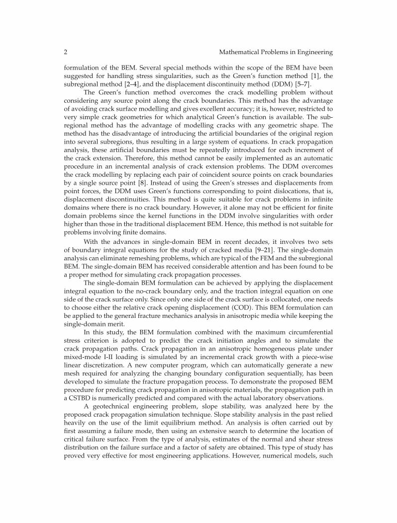
For anisotropic materials, the general form of the elastic stress field near the crack tipin the local Cartesian coordinates x”-y”, as shown in Figure 3, can be expressed in terms ofthe two SIFs KI and KII as follows [29]:
σx′′ =KI√2πr
Re
[μ1μ2
μ1 − μ2
(μ2√
cos θ + μ2 sin θ− μ1√
cos θ + μ1 sin θ
)]
+KII√2πr
Re
[1
μ1 − μ2
(μ2
2√cos θ + μ2 sin θ
− μ21√
cos θ + μ1 sin θ
)],
10 Mathematical Problems in Engineering
σy′′ =KI√2πr
Re
[1
μ1 − μ2
(μ1√
cos θ + μ2 sin θ− μ2√
cos θ + μ1 sin θ
)]
+KII√2πr
Re
[1
μ1 − μ2
(1√
cos θ + μ2 sin θ− 1√
cos θ + μ1 sin θ
)],
τx′′y′′ =KI√2πr
Re
[μ1μ2
μ1 − μ2
(1√
cos θ + μ1 sin θ− 1√
cos θ + μ2 sin θ
)]
+KII√2πr
Re
[1
μ1 − μ2
(μ1√
cos θ + μ1 sin θ− μ2√
cos θ + μ2 sin θ
)],
(2.23)
where μ1 and μ2 are the roots of (2.1). We have
σθ =σx′′ + σy′′
2− σx′′ − σy′′
2cos 2θ − τx′′y′′ sin 2θ,
τrθ = −σx” − σy”
2sin 2θ + τx”y” cos 2θ.
(2.24)
For the σ-criterion, the angle of crack initiation, θ0, must satisfy the following:
∂σθ∂θ
= 0 (or τrθ = 0),∂2σθ∂θ2
< 0. (2.25)
A numerical procedure is applied to find the angle θ0 when σθ is maximum for knownvalues of the material elastic constants, the anisotropic orientation angle ψ, and the crackgeometry.
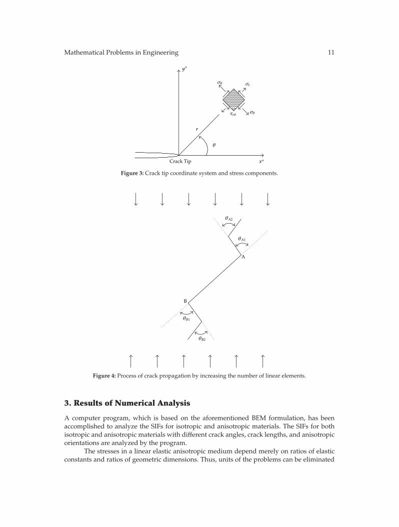
Since the proposed BEM formulation is simple and can be used for any kind of crackgeometry, it is straightforward to extend to analyze the crack propagation in anisotropicmaterials. The process of crack propagation in anisotropic homogeneous material undermixed mode I-II loading is simulated by incremental crack extension with a piecewise lineardiscretization. For each incremental analysis, the crack extension is conveniently modeled bya new boundary element. A computer program has been developed to automatically generatenew data required for sequentially analyzing the changing boundary configuration. Based onthe calculation of the SIFs and crack initiation angle for each increment, the procedure of crackpropagation can be simulated. The steps in the crack propagation process are summarized asfollows (Figure 4):
(1) compute the SIFs using the proposed BEM formulation;
(2) determine the angle of crack initiation based on the maximum circumferential stresscriterion;
(3) extend the crack by a linear element (of length selected by the user) along thedirection determined in step (2);
(4) automatically generate the new BEM mesh;
(5) repeat all of the above steps until the crack is near the outer boundary.
Mathematical Problems in Engineering 11
Crack Tip
r
σθ
σθ
σr
τrθ
θ
x′′
y′′
Figure 3: Crack tip coordinate system and stress components.
θA2
θA1
θB1
θB2
A
B
Figure 4: Process of crack propagation by increasing the number of linear elements.
3. Results of Numerical Analysis
A computer program, which is based on the aforementioned BEM formulation, has beenaccomplished to analyze the SIFs for isotropic and anisotropic materials. The SIFs for bothisotropic and anisotropic materials with different crack angles, crack lengths, and anisotropicorientations are analyzed by the program.
The stresses in a linear elastic anisotropic medium depend merely on ratios of elasticconstants and ratios of geometric dimensions. Thus, units of the problems can be eliminated
12 Mathematical Problems in Engineering
y
W
β
2a
R
W
Figure 5: The geometry of cracked Brazilian disc.
by the method of normalization. Accordingly, the SIFs of the following examples arenormalized with respect to the applied load and to the square root of half crack length.
Totally 9 numerical examples including isotropic and anisotropic materials arepresented to illustrate the accuracy and versatility of the proposed BEM program fordetermining the SIFs, predicting the crack initiation angle, and simulating crack propagationpath. The examples include cases for finite/infinite domains, curved/edge cracks, andisotropic/anisotropic conditions. A generalized plane stress is assumed in all the examplesexcept for crack propagation simulation of slope failure.
3.1. Stress Intensity Factors Determination
Example 1: Isotropic Cracked Brazilian Disc
In order to compare our results with the existing published results, an isotropic and crackedBrazilian disc with a central slant crack is considered. The geometry of the problem is thatof a thin circular disc of radius R and thickness t with a central crack of length 2a, loadedwith a pair of concentrated and diametral compressive load W , as shown in Figure 5. Theouter boundary and crack surface are discretized with 28 continuous and 10 discontinuousquadratic elements, respectively. Two cases are analyzed: (1) a/R = 0.5, the crack angleβ varies between 0 and π/2, and (2) β = 45◦, a/R varies between 0.1 and 0.7. The twonormalized SIFs, FI(= KI/σ
√πa) and FII(= KII/σ
√πa), calculated with the BEM program
for these two cases, are compared with those obtained numerically by Atkinson et al. [42]and Chen et al. [28]. The results are shown in Tables 1 and 2. In general, a good agreement isfound among these three methods.
Mathematical Problems in Engineering 13
Table 1: Normalized SIFs for a central slant in an isotropic Brazilian disc subjected to a concentrated load(a/R = 0.5).
β (rad.) Atkinson et al. (1982) [42] Chen et al. (1998) [28] This studyKI/σ
Consider a circular-arc crack of a radius R embedded in an infinite domain under a far-fieldtensile stress σ and out-of-plane shear stress τ as shown in Figure 6. The center of the circulararc is taken at the origin of the coordinate system, the midpoint of the crack is located onthe x-axis, and the angle subtended by the crack is 2α. In this example only 20 discontinuousquadratic elements are used to discretize the curved crack surface. For α = 30◦ and α = 45◦,the numerical solutions of SIFs calculated by this study as well as the analytic ones by Tadaet al. [43] are shown in Table 3.
Example 3: Anisotropic Rectangular Plate under a Uniform Tension
In order to evaluate the influence of material anisotropy on the SIFs, consider an anisotropicrectangular plate of width 2w, and height 2h with a central crack inclined 45◦ to the x-axis,as shown in Figure 7. The plate is loaded with a uniform tensile stress in the y direction. Theratios of crack length and of height to width are a/W = 0.2 and h/W = 2.0, respectively.The material is glass-epoxy with elastic properties E = 48.26 GPa, E′ = 17.24 GPa, ν′ = 0.29,and G′ = 6.89 GPa. The direction of the fibers is rotated from ψ = 0◦ to ψ = 180◦. Theouter boundary and crack surface are discretized with 32 continuous and 10 discontinuousquadratic elements, respectively. Table 4 shows the results obtained by the proposed method
14 Mathematical Problems in Engineering
α α
a
Y
X
σ
σ
τ
τ
Figure 6: A curved crack under a far-field tensile stress σ and out-of-plane shear stress τ .
Table 3: Normalized SIFs for a circular arc crack in an infinite domain.
as well as those by Sollero and Aliabadi [44], Gandhi [45], and Chen et al. [28]. Again, anexcellent agreement is obtained.
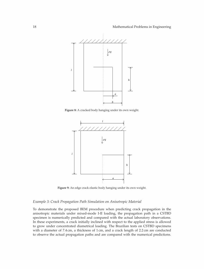
Example 4: Cracked Body Hanging under Its Own Weight
Consider a body with a crack of length 2a under the gravitational loading as shown inFigure 8. The ratios of distance from crack to free end to height are h/l = 0.5. The ratio ofcrack length to width is varied from 0.05 to 0.5. The outer boundary and crack surface arediscretized with 44 continuous and 30 discontinuous quadratic elements, respectively. Planestrain condition is considered. Table 5 shows the results obtained by the proposed methodas well as the analytic ones by Shi’s handbook [46], and the numerical ones by Ostanin et al.(2011) [47]. Again, an excellent agreement is obtained.
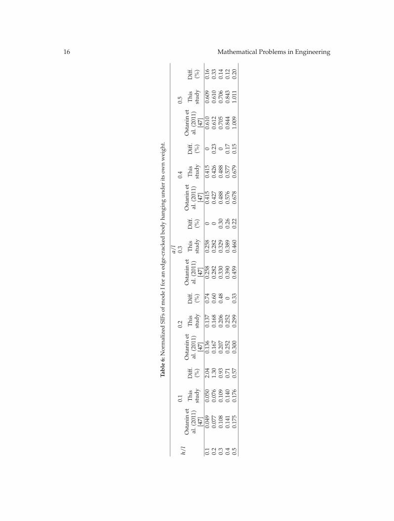
Example 5: Edge Crack in an Elastic Body Hanging under Its Own Weight
Figure 9 shows a square block l × l containing an edge crack of length a is hanging under itsown weight. The distance of crack tip to the free end is h. Poisson’s ratio is assumed to be zero.In this example, the outer boundary and crack surface are discretized with 44 continuous and30 discontinuous quadratic elements, respectively. Table 6 shows the normalized SIFs of modeI. This problem was solved previously by Ostanin et al. (2011) [47] using a complex variableboundary element method (CVBEM). As shown in Table 6, the present numerical results arein excellent agreement with those obtained by Ostanin et al. (2011) [47].
Mathematical Problems in Engineering 15
Table 4: Normalized SIFs for a central slant in anisotropic rectangular plate subjected to a uniform tension(β = 45◦, a/R = 0.5).
ψ(Deg.)
Gandhi (1972) [45] Sollero and Aliabadi(1995) [15]
3.2. Crack Initiation Angle Prediction and Propagation Path Simulation
The proposed BEM formulation combined with the maximum circumferential stress criterionis developed to predict the angle of crack initiation and to simulate the path of crackpropagation under mixed-mode loading. The crack propagation process in the crackedmaterials is numerically estimated by two-dimensional stress and displacement analysis. Inorder to understand the behavior of cracks under mixed-mode loading, the BEM program isapplied.
Example 1: Crack Initiation Angle Prediction
The proposed BEM formulation is also used to predict the initial growth of cracks inanisotropic materials. To examine the validity of our crack initiation prediction procedure,the tests of Erdogan and Sih [35] and Vallejo [40] are reproduced numerically with our BEMprogram. Erdogan and Sih [35] conducted uniaxial tension test on isotropic Plexiglass sheets229 × 457 × 4.8 mm in size containing a 50.8 mm central crack. The crack inclination angle βbetween the crack plane and the tensile stress is varied. Figure 10 shows the variation of thecrack initiation angle θ0 with the crack angle β determined numerically and experimentally.
16 Mathematical Problems in Engineering
Table
6:N
orm
aliz
edSI
Fsof
mod
eIf
oran
edge
-cra
cked
bod
yha
ngin
gun
der
its
own
wei
ght.
h/l
a/l
0.1
0.2
0.3
0.4
0.5
Ost
anin
etal
.(20
11)
[47]
Thi
sst
udy
Diff
.(%
)
Ost
anin
etal
.(20
11)
[47]
Thi
sst
udy
Diff
.(%
)
Ost
anin
etal
.(20
11)
[47]
Thi
sst
udy
Diff
.(%
)
Ost
anin
etal
.(20
11)
[47]
Thi
sst
udy
Diff
.(%
)
Ost
anin
etal
.(20
11)
[47]
Thi
sst
udy
Diff
.(%
)
0.1
0.04
90.
050
2.04
0.13
60.
137
0.74
0.25
80.
258
00.
415
0.41
50
0.61
00.
609
0.16
0.2
0.07
70.
076
1.30
0.16
70.
168
0.60
0.28
20.
282
00.
427
0.42
60.
230.
612
0.61
00.
330.
30.
108
0.10
90.
930.
207
0.20
60.
480.
330
0.32
90.
300.
488
0.48
80
0.70
50.
706
0.14
0.4
0.14
10.
140
0.71
0.25
20.
252
00.
390
0.38
90.
260.
576
0.57
70.
170.
844
0.84
30.
120.
50.
175
0.17
60.
570.
300
0.29
90.
330.
459
0.46
00.
220.
678
0.67
90.
151.
009
1.01
10.
20
Mathematical Problems in Engineering 17
σ
2 W
y
2 h
2 ax
Ψ45◦
Figure 7: An anisotropic rectangular plate with a central crack inclined 45◦ under uniform tensile stress σ.
A good agreement is found between the experimental results of Erdogan and Sih [35] andour numerical predictions.
Other verification is done using the experimental results of Vallejo [40]. The uniaxialcompression tests were conducted on cracked prismatic specimens of kaolinite clay 76.2 ×76.2 × 25.4 mm in size containing a central crack 24.9 mm in length by Vallejo [40].Several tests are carried out by varying the crack angle β between the crack plane andthe compressive stress. Figure 11 shows a comparison between the crack initiation anglesmeasured experimentally and those predicted numerically. Again, a good agreement is foundwith the experimental results.
Example 2: Isotropic Cracked Plate under Pure Mode I Loading
The behavior of an existing crack under pure mode I loading is studied for the application.The first problem, as shown in Figure 12, is a square plate with a horizontal edge cracksubjected to uniaxial tension. The width of the square plate is w. The initial crack length, a,is equal to w/3. The no-crack boundary and crack surface are discretized with 55 continuousand 10 discontinuous quadratic elements, respectively. According to the experimental resultsfrom Erdogan and Sih [35], it is known that the crack propagation angle (θ) is zero whenthe crack inclination angle (β) is 90 degree with respect to y-axis, which means that the crackwill propagate along the horizontal direction. Figure 13 shows the path of crack propagationunder pure mode I loading. It is shown that the path of crack propagation is a horizontal line,which is in full agreement with the experimental results made by Erdogan and Sih [35].
18 Mathematical Problems in Engineering
a
b
h
l
ρg
Figure 8: A cracked body hanging under its own weight.
a
h
l
l
ρg
Figure 9: An edge crack elastic body hanging under its own weight.
Example 3: Crack Propagation Path Simulation on Anisotropic Material
To demonstrate the proposed BEM procedure when predicting crack propagation in theanisotropic materials under mixed-mode I-II loading, the propagation path in a CSTBDspecimen is numerically predicted and compared with the actual laboratory observations.In these experiments, a crack initially inclined with respect to the applied stress is allowedto grow under concentrated diametrical loading. The Brazilian tests on CSTBD specimenswith a diameter of 7.4 cm, a thickness of 1 cm, and a crack length of 2.2 cm are conductedto observe the actual propagation paths and are compared with the numerical predictions.
Mathematical Problems in Engineering 19
00
10 20 30 40 50 60 70 80 90
−10
−20
−30
−40
−50
−60
−70
−80
This study
Cra
ck in
itia
tion
ang
le,θ
0(◦)
β
θ0
σ
σ
Crack angle β (◦)
Erdogan and Sih (1963) [35]
Figure 10: Variation of crack initiation angle θ0 with the crack angle β. Plexiglass plate subjected to uniaxialtension.
0
20
40
60
80
100
120
140
160
180
0 10 20 30 40 50 60 70 80 90
Numerical results (this study)
Experimental results (Vallejo, 1987) [40]
Cra
ck in
itia
tion
ang
le,θ
0(◦)
Crack angle, β
β
(◦)
Water content, w = 3%w = 9%
θ0
σ
σ
Figure 11: Variation of crack initiation angle θ0 with the crack angle β. Prismatic sample of kaolinite claysubjected to uniaxial compression.
Details of the experimental procedure can be found in the paper by Ke et al. [48]. The fiveelastic constants of anisotropic marble are E = 78.302 GPa, E′ = 67.681 GPa, ν = 0.267,ν′ = 0.185, G = 30.735 GPa, and G′ = 25.336 GPa, respectively. The ratios of E/E′ and E/G′ are1.156 and 3.091, respectively. Since the value of E/E′ = 1.156, this marble can be classified asa slightly anisotropic rock.
Two specimens with the material inclination angle ψ = 45◦, defined as the AM-4,and DM-4, have crack angles β = 0◦ and β = 45◦ respectively. After Brazilian tests withcracked specimens, the paths of crack propagation for AM-4 and DM-4 are shown in Figures14 and 16, respectively. It can be observed that the crack propagates nearly perpendicular
20 Mathematical Problems in Engineering
W
a
σ
σ
W/
2W/
2
Figure 12: Square plate with a straight edge crack under pure mode I loading.
Simulation of propagation path
Figure 13: Crack propagation path and normalized SIFs of the cracked plate initially under pure mode Iloading.
to the crack surface in the initial stage and then rapidly approaches toward the loadingpoint. The proposed BEM procedure is also used to simulate crack propagation in the CSTBDspecimens. The outer boundary and crack surface are discretized with 28 continuous and20 discontinuous quadratic elements, respectively. Figures 15 and 17 are the comparisons ofcrack propagation paths between experimental observations and numerical predictions inAM4 and DM-4, respectively. Again, the proposed BEM procedure accurately simulates the
Mathematical Problems in Engineering 21
Figure 14: Photograph of specimen AM-4 after failure (ψ = 0◦ and β = 45◦).
Numerical resultExperimental result
Ψ = 0, β = 45
Figure 15: Propagation of a crack at the center of a CSTBD specimen with ψ = 0◦ and β = 45◦. Comparisonbetween experimental observations and numerical predictions for specimen AM-4.
crack propagation in these anisotropic specimens. According to the simulations of foregoingexamples, it can be concluded that the proposed BEM is capable of predicting the crackpropagation in anisotropic rocks.
3.3. Crack Propagation Simulation of Slope Failure
A slope 15 m high with a 2 m deep initial tension crack located on the top of the slope isused for the analysis. 10 discontinuous quadratic elements and 46 quadratic elements wereused to discretize the crack surface and outer boundary. Plane strain condition is considered.The top of the slope has surface recharge due to heavy rain. Figure 18 gives a descriptionof the problem layout that includes the slope geometry and the crack. The crack propagation
22 Mathematical Problems in Engineering
Figure 16: Photograph of specimen DM-4 after failure (ψ = 45◦ and β = 45◦).
Numerical resultExperimental result
Ψ = 45, β = 45
Figure 17: Propagation of a crack at the center of a CSTBD specimen with ψ = 45◦ and β = 45◦. Comparisonbetween experimental observations and numerical predictions for specimen DM-4.
20 m
10 m(2 m )
15 m
2 m
Tension crack
Ψ
Figure 18: The description of an anisotropic rock slope.
Mathematical Problems in Engineering 23
Ψ = 0Ψ = 15Ψ = 30Ψ = 45
Ψ = 60Ψ = 75Ψ = 90
Figure 19: The anisotropic rock slope failure surface simulated by the proposed BEM.
process under body force of gravity is considered. The crack increment length is fixed at a size1/6 times the crack tip element. An anisotropic rock slope was simulated with different valuesof rock anisotropy (ψ = 0◦, 15◦, 30◦, 45◦, 60◦, 75◦, 90◦). The dimensionless elastic constant(E/E′ = 3) is considered. Figure 18 gives a description of the problem layout that includesthe slope geometry, the crack, and anisotropy orientation. Figure 19 shows the slope failuresurfaces simulated by the BEM. It can be found that the slope failure surfaces depend onthe different anisotropy inclination angles. The anisotropy orientation angle ψ has a stronginfluence on the surface of slope failure.
4. Conclusions
A formulation of the BEM, based on the relative displacements near the crack tip, isutilized to determine the mixed-mode SIFs of anisotropic rocks. Numerical examples for thedetermination of the mixed-mode SIFs for a CSTBD specimen are presented for isotropicand anisotropic media. The numerical results obtained by the proposed method are in goodagreement with those reported by previously published results. In addition, the SIFs forvarious crack geometry and loading type such as a curved crack under far-field tensilestress and a cracked body hanging by its own weight are also determined by the proposedBEM formulation. The numerical results obtained by this study are in agreement with thosereported by previously published results.
This paper presents the development of BEM procedure based on the maximumcircumferential stress criterion for predicting the crack initiation directions and propagationpaths in isotropic and anisotropic materials under mixed-mode loading. Good agreements arefound between crack initiation and propagation predicted with the BEM and experimentalobservations reported by previous researchers of isotropic materials. Numerical simulationsof crack initiation and propagation in CSTBD specimens of the anisotropic rock are also foundto compare well with experimental results. Additionally, the crack propagation simulationtechnique is used to apply for analyzing the rock slope within a preexisting tensile crack. Wecan find that the slope failure surfaces strongly depend on the different anisotropy inclinationangles.
24 Mathematical Problems in Engineering
Nomenclature
β: The crack inclination angle [deg.]ψ: The material orientation angle [deg.]a: The half crack lengthCSTBD: The cracked straight through Brazilian discD: The diameter of Brazilian discE: The Young’s modulusSIF(s): The Stress Intensity Factor(s)KI: The mode I SIF [MPa m1/2]KII: The mode II SIF [MPa m1/2]FI: The normalized mode I SIFFII: The normalized mode II SIF.
Acknowledgments
The authors are grateful to the Editor, Dr. Kue-Hong Chen, and an anonymous reviewer forconstructive comments that led to improvements of the paper.
References
[1] M. D. Snyder and T. A. Cruse, “Boundary-integral equation analysis of cracked anisotropic plates,”International Journal of Fracture, vol. 11, no. 2, pp. 315–328, 1975.
[2] G. E. Blandford, A. R. Ingraffea, and J. A. Liggett, “Two-dimensional stress intensity factor computa-tions using the boundary element method,” International Journal for Numerical Methods in Engineering,vol. 17, no. 3, pp. 387–404, 1981.
[3] P. Sollero and M. H. Aliabadi, “Fracture mechanics analysis of anisotropic plates by the boundaryelement method,” International Journal of Fracture, vol. 64, no. 4, pp. 269–284, 1993.
[4] P. Sollero, M. H. Aliabadi, and D. P. Rooke, “Anisotropic analysis of cracks emanating from circularholes in composite laminates using the boundary element method,” Engineering Fracture Mechanics,vol. 49, no. 2, pp. 213–224, 1994.
[5] L. L. Libatskii and S. E. Kovchik, “Fracture of discs containing cracks,” Soviet Materials Science, vol. 3,no. 4, pp. 334–339, 1967.
[6] S. L. Crouch and A. M. Starfield, Boundary Element Methods in Solid Mechanics, George Allen andUnwin, London, UK, 1983.
[7] B. Shen and O. Stephansson, “Modification of the G-criterion for crack propagation subjected tocompression,” Engineering Fracture Mechanics, vol. 47, no. 2, pp. 177–189, 1994.
[8] A. Portela, Dual Boundary Element Analysis of Crack Growth, UK and USA: Computational Mechanics,Boston, Mass, USA, 1993.
[9] M. H. Aliabadi, “A new generation of boundary element methods in fracture mechanics,” InternationalJournal of Fracture, vol. 86, no. 1-2, pp. 91–125, 1997.
[10] A. Portela, Dual Boundary Element Analysis of Crack Growth, Computational Mechanics, Boston, Mass,USA, 1993.
[11] H. K. Hong and J. T. Chen, “Derivations of integral equations of elasticity,” Journal of EngineeringMechanics, vol. 114, pp. 1028–1044, 1988.
[12] L. J. Gray, L. F. Martha, and A. R. Ingraffea, “Hypersingular integrals in boundary element fractureanalysis,” International Journal for Numerical Methods in Engineering, vol. 29, no. 6, pp. 1135–1158, 1990.
[13] A. Portela, M. H. Aliabadi, and D. P. Rooke, “Dual boundary element method. Effectiveimplementation for crack problems,” International Journal for Numerical Methods in Engineering, vol.33, no. 6, pp. 1269–1287, 1992.
[14] A. Portela, M. H. Aliabadi, and D. P. Rooke, “Dual boundary element incremental analysis of crackpropagation,” Computers and Structures, vol. 46, no. 2, pp. 237–247, 1993.
Mathematical Problems in Engineering 25
[15] P. Sollero and M. H. Aliabadi, “Dual boundary element analysis of anisotropic crack problems,” inBoundary Element XVII, pp. 267–278, Computational Mechanics, Southampton, UK, 1995.
[16] P. Sollero and M. H. Aliabadi, “Anisotropic analysis of cracks in composite laminates using the dualboundary element method,” Composite Structures, vol. 31, no. 3, pp. 229–233, 1995.
[17] E. Pan and B. Amadei, “Fracture mechanics analysis of cracked 2-D anisotropic media with a newformulation of the boundary element method,” International Journal of Fracture, vol. 77, no. 2, pp. 161–174, 1996.
[18] E. Pan, “A general boundary element analysis of 2-D linear elastic fracture mechanics,” InternationalJournal of Fracture, vol. 88, no. 1, pp. 41–59, 1997.
[19] J. T. Chen and H. K. Hong, “Review of dual boundary element methods with emphasis on hyper-singular integrals and divergent series,” Applied Mechanics Reviews, vol. 52, no. 1, pp. 17–32, 1999.
[20] A. P. Cisilino and M. H. Aliabadi, “Three-dimensional boundary element analysis of fatigue crackgrowth in linear and non-linear fracture problems,” Engineering Fracture Mechanics, vol. 63, no. 6, pp.713–733, 1999.
[21] S. W. Chyuan and Lin Jiann-Hwa, “Dual boundary element analysis for fatigue behavior of missilestructures,” Journal of the Chinese Institute Engineers, vol. 23, no. 3, pp. 339–348, 2000.
[22] E. C. Kalkani and D. R. Piteau, “Finite element analysis of toppling failure at Hell’s Gate Bluffs. BritishColumbia,” Bulletin of the International Association of Engineering Geology, vol. 13, no. 4, pp. 315–327,1976.
[23] J. Krahn and N. R. Morgenstern, “The mechanics of the Frank Slide. Rock Engineering forFoundations and Slopes,” in Proceedings of the ASCE Geotechnical Engineering Specialty Conference, pp.309–332, ASCE, Boulder, Colo, USA, 1976.
[24] T. R. Stacey, Y. Xianbin, R. Armstrong, and G. J. Keyter, “New slope stability considerations for deepopen pit mines,” Journal of The South African Institute of Mining and Metallurgy, vol. 103, no. 6, pp.373–389, 2003.
[26] J. S. Coggan, D. Stead, and J. H. Howe, “Characterisation of a structurally controlled flowslide ina kaolinised granite slope,” in Proceedings of the 8th International Symposium on Landslides, Landslidesin Research, Theory and Practice, E. Bromhead, N. Dixon, and M.-L. Ibsen, Eds., vol. 1, pp. 299–304,Cardiff, UK, 2000.
[27] D. Stead, E. Eberhardt, and J. S. Coggan, “Developments in the characterization of complex rock slopedeformation and failure using numerical modelling techniques,” Engineering Geology, vol. 83, no. 1–3,pp. 217–235, 2006.
[28] C. S. Chen, E. Pan, and B. Amadei, “Fracture mechanics analysis of cracked discs of anisotropic rockusing the boundary element method,” International Journal of Rock Mechanics and Mining Sciences, vol.35, no. 2, pp. 195–218, 1998.
[29] G. C. Sih, P. C. Paris, and G. R. Irwin, “On cracks in rectilinearly anisotropic bodies,” InternationalJournal of Fracture Mechanics, vol. 1, no. 3, pp. 189–203, 1965.
[30] Z. Suo, “Singularities, interfaces and cracks in dissimilar anisotropic media,” in Proceedings of the RoyalSociety of London, Series A, Mathematical and Physical Sciences, pp. 331–358, 1990.
[31] T. C. T. Ting, Anisotropic Elasticity: Theory and Applications, Oxford University Press, New York, NY,USA, 1996.
[32] M. H. Aliabadi, “Boundary element formulations in fracture mechanics,” Applied Mechanics Reviews,vol. 50, no. 2, pp. 83–96, 1997.
[33] M. Cerrolaza and E. Alarcon, “Bi-cubic transformation for the numerical evaluation of the CauchyPrincipal Value integrals in boundary methods,” International Journal for Numerical Methods inEngineering, vol. 28, no. 5, pp. 987–999, 1989.
[34] E. Pan, C. S. Chen, and B. Amadei, “A BEM formulation for anisotropic half-plane problems,” Engi-neering Analysis with Boundary Elements, vol. 20, no. 3, pp. 185–195, 1997.
[35] F. Erdogan and G. C. Sih, “On the crack extension in plates under loading and transverse shear,”Journal of Basic Engineering, vol. 85, pp. 519–527, 1963.
[36] K. Palaniswamy and W. G. Knauss, “Propagation of a crack under general, in-plane tension,”International Journal of Fracture Mechanics, vol. 8, no. 1, pp. 114–117, 1972.
[37] G. C. Sih, “Strain-energy-density factor applied to mixed mode crack problems,” International Journalof Fracture, vol. 10, no. 3, pp. 305–321, 1974.
[38] C. W. Woo and L. H. Ling, “On angled crack initiation under biaxial loading,” Journal of Strain Analysisfor Engineering Design, vol. 19, no. 1, pp. 51–59, 1984.
26 Mathematical Problems in Engineering
[39] H. A. Richard, “Examination of brittle fracture criteria for overlapping mode I and mode II loadingapplied to cracks,” in Application of Fracture Mechanics to Materials and Structures, G. C. Sih et al., Ed.,pp. 309–316, Martinus Nijhoff, 1984.
[40] L. E. Vallejo, “The brittle and ductile behavior of a material containing a crack under mixed-modeloading,” in Proceedings of the 28th U.S. Symposium on Rock Mechanics, University of Arizona, Tucson,Ariz, USA, 1987.
[41] B. N. Whittaker, R. N. Singh, and Gexin Sun, Rock Fracture Mechanics: Principles, Design and Applica-tions, Academic Press, Amsterdam, The Netherlands, 1992.
[42] C. Atkinson, R. E. Smelser, and J. Sanchez, “Combined mode fracture via the cracked Brazilian disktest,” International Journal of Fracture, vol. 18, no. 4, pp. 279–291, 1982.
[43] H. Tada, P. C. Paris, and G. R. Irwin, The Stress Analysis of Cracks Handbook, Paris Productions Incor-porated, Missouri, Mo, USA, 1985.
[44] P. Sollero and M. H. Aliabadi, “Fracture mechanics analysis of anisotropic plates by the boundaryelement method,” International Journal of Fracture, vol. 64, no. 4, pp. 269–284, 1993.
[45] K. R. Gandhi, “Analysis of inclined crack centrally placed in an orthotropic rectangular plate,” Journalof Strain Analysis, vol. 7, no. 3, pp. 157–162, 1972.
[46] G. C. Sih, Handbook of Stress-Intensity Factors: Stress-Intensity Factor Solutions and Formulas for Reference,Lehigh University, Bethlehem, Pa, USA, 1973.
[47] I. A. Ostanin, S. G. Mogilevskaya, J. F. Labuz, and J. Napier, “Complex variables boundary elementmethod for elasticity problems with constant body force,” Engineering Analysis with BoundaryElements, vol. 35, no. 4, pp. 623–630, 2011.
[48] C. C. Ke, C. S. Chen, and C. H. Tu, “Determination of fracture toughness of anisotropic rocks byboundary element method,” Rock Mechanics and Rock Engineering, vol. 41, no. 4, pp. 509–538, 2008.