JOURNAL OF GEOPHYSICAL RESEARCH, VOL. 107, NO. 8 4, 2065, IO.l029/200IJ8 000191, 2002

Two-dimensional magnetotelluric inversion of blocky geoelectrical structures

S. Mehanee and M. Zhdanov Department of Geology and Geophysics , University of Utah, Salt Lake City, Utah, USA

Received 30 November 1999; revised 16 October 2000; accepted 22 August 2001; published 13 April 2002.

[ I] This paper de mo ns trates that there are alternative ap proa ches to the magneto telluric (M T) inverse problem so lution based on different types of geoelectrical mod els. The traditional approach uses smooth models to describe the conductivity d istribution in underground formations. In this paper, we prese nt a new approach, based on approxi mating the geology by models with blo cky co nd uct ivi ty structures. We can se lect one or ano the r class of inverse mod els by choosing between differe nt stabilizing functionals in the reg ularization metho d. The fina l decision , w hose approach may be used for the specific MT data se t, is made on the basis of available geo log ica l information . This paper describes a new way of stabi liz ing two -dimens iona l MT inversion using a minimum support functiona l and shows the improvement that it provides over traditiona l meth ods for geoelec trical mo de ls with blocky structures. The new meth od is applied to MT data co llec ted for crus ta l imaging in the Carrizo Plain in Californ ia and to MT data co llec ted for mining exploration by INc a Exploration . INDEX TERMS : 0644 Elec tro magnetics : N umerica l me thods; 3260 Mathematical Geophysics : Inverse theory; K EYWORDS: Electromagnetic , m agnetotelluric, inversion, foc using

1. Introduction about the geological structure in the inversion procedure. In the case of the traditional smooth inversion this information is provided as

[2J The two-dimensional (2-D) magnetotelluric inverse problem an assumption that the solution, the geoelectrical model in the MT has been addressed by several authors. The most well-known case, should be represented by smooth functions. At the same time, approaches are the search for a smooth model [de Groot-Hedlin in some geological situations it can be useful to consider other and Constable, 1990; de Lugao et al., 1997; Mackie et aI., 1997; assumptions in selecting the class of possible solutions. For Rodi and Mackie, 2001] and the rapid relaxation inversion (RRI) example, the traditional smooth inversion algorithms have difficul­[Smith and Booker, 1991). The majority of existing algorithms are ties in describing the sharp geoelectrical boundaries between differ­based on the minimum norm or maximum smoothness criteria used ent geological formations, while in actual geological situations, for stable inversion of magnetotelluric data. The RRI method is sharp boundaries may constitute an important goal of interpretation. also based on approximate calculation of the Frechet derivatives This problem arises in inversion for a local conductive target with a under the assumption that horizontal variations in conductivity are sharp boundary embedded in a resistive host rock, which is a typical much smaller than vertical ones. model in mining exploration. Another example is a marine MT

[3J The magnetotelluric (MT) inverse problem, as almost any survey to map the salt dome structures in sea bottom geological inverse problem in geophysics, is ill-posed and therefore unstable. formations [Hoversten et al., 1998). Even in general cases of It means that one can find several very different geoelectrical regional geological studies we may be interested in determining models fitting the observed data with the same accuracy. The stable large regions with blocky structures. In these situations it can be solution of an ill-posed inverse problem can be obtained by using useful to search for a stable solution within the class of inverse the corresponding regularization methods [Tikhonov and Arsenin, models with blocky geoelectrical structures . The mathematical 1977J. The regularization is based on a simple idea ofsearching for technique for solving this problem was developed by Portniaguine a solution within the specific class of selected models. Note that the and Zhdanov [1999a). It is based on introducing a new type of traditional way to implement regularization in inverse problem stabilizing functional in inverse problem solution, a so-called solution is based on considering the class of inverse models with minimum support functional. We call this technique a focusing smooth distribution of model parameters. Within the framework of regularized inversion to distinguish it from the traditional smooth the classical Tikhonov regularization, one can select the smooth regularized inversion. solution by introducing the corresponding minimum norm, or [5J This technique was successfully applied to the inversion of " smoothing" stabilizing functionals. This approach is widely used gravity data [Last and Kubik, 1983; Portniaguine and Zhdanov, in geophysics and has been proved to be a powerful tool for stable 1999aJ to generate a focused and resolved inverse image of the inversion of geophysical data. Note that practically all traditional density distribution in a geological cross section. This idea was MT inversion methods use the same approach and therefore they also implemented in inversion of three-dimensional (3-D) con­produce a smooth image of geoelectrical structures, which in some trolled-source MT (CSMT) data over the structures with sharp cases may not describe the geology properly. geoelectrical boundaries [Portniaguine and Zhdanov, 1999b; Zhda­

[4] It is important to emphasize, however, that regularization nov and Hursan, 2000]. In this paper we demonstrate that this does not necessarily mean a smoothing of the solution. The main approach helps to generate much more "focused" and resolved basis for regularization is the implementation ofa priori information images of blocky geoelectrical structures than conventional MT

inversion methods. Copyright 2002 by the American Geophysical Union. [6J We test the focused regularized inversion of magnetotelluric 0148-0227/02/200IJBOOO 191$09.00 data on synthetic models. We also apply this technique to interpret

EPM 2 - I

EPM 2 - 2 MEHANE E AN D ZHD ANO V: MT INVERSION OF BLOCKY STRUCTU RES

the MT data collected in Canizo Plain, California [Unsworth et al., 1999], and to analyze the MT data collected for mining exploration by INCO Explorat ion.

2. Principles of Blocky Structure Imaging

[7] The magnetotelluric inverse problem can be formul ated as the numerica l solution of the following operator equation:

A(m) = d, ( 1)

where A is the forward modeling operator, m = mer) is a scalar function describing geoelec trical model parame ter distribu tion, conductivit ies a(r) (or resistivities per)), in some volume Vin the Earth, (m E M, where M is a Hilb ert space of model parameters with an Lz norm), and d is a geophysica l data set (d E D, where D is a Hilbert space of data). Inverse problem (1) is usually ill-posed; that is, the so lution can be nonunique and unstabl e. The conventiona l way of solving ill-posed inverse problems, according to regularization theory [Tikhonov and Arsenin, 1977; Zhdanov, 1993], is based on minimization of the Tikhonov parametric functional:

(2)PO«m ) = <jJ(m) + os (m),

where <jJ(m) is a misfit functional determined as a square norm of difference between observed and predicted (theoretical) data,

<jJ(m) = II Am - d 111 , (3)

and sCm) is a stabilizing functional (a stabilizer). The main role of the stabilizer is to select an appropriate class of models for the inverse problem solution. Actually, the stabilizer can be treated as a tool for including a priori inform ation about the geological struc tures in the inverse problem solution.

[8] There are several comm on choices for stabilizers, wh ich lead to the different classes of geologica l models used for inver­sion. One is based on the least squares criteria or, in other words , on the Lz norm for funct ions desc ribing geoe lectrica l model parameters:

SL, (m) = II mllz= (m,m) = 1mZdv = min , (4)

whe re ( , ) deno tes the inner product multipli cation [Parker, 1994] . Another stabi lizer uses a minimum norm of difference between the selected model and some a priori model mapr:

SL,apr(m) = 11 m - maprW= min . (5)

The conventional maximum smoo thness stabilizing functional uses the minimum norm of the gradient of model parameters 'ilm :

z=Smaxsm(m) = II 'il mll ('ilm, 'ilm) = min , (6)

or, in some cases , the minimum norm of the Laplaci an of mod el parameters 'ilZm,

Smaxsm(m) = II'ilZmIIZ= ('ilZm, 'ilZm) = min. (7)

The se functionals have been successfully used in many inversion schemes developed for EM data interpretation [Berdichevsky and Zhdanov, 1984; Constable et al., 1987; Jiracek et al., 1987; Smith and Booker, 1991; Ellis and Oldenburg, 1994 ; Rodi and Mackie,

2001]. These stabilizers produce smoot h geoe lectrica l models which in some practical situations may not desc ribe properly the real blocky geological structures with sharp bound aries.

[9] Last and Kubik [1983] and Portniaguine and Zhdanov [1999a] considered a different stabilizing functional which mini­mizes the area of the anomalous model parameters. This functiona l is called a minimum support (MS) functiona l, which can be described as follows. Consider the following integral of the model parameter distribution:

r~dv,Je(m) = Jv mZ+ eZ (8)

where e =F 0 is a small numb er, introduced to exclude singularity in the points where m = O.

[1 0] We introduce the support of m (denoted sptm) or mod el parameter support, as the combined closed subdomai ns of V where m =F O. Then (8) can be modified:

Je(m) =l [ 1 -~] dv=sPtm - eZl ~dv . (9) sptm m + e splm m + e

From (8) we can see that

Je(m) -> sptm, e -> O. (10)

Thus Je(m) can be treated as a functional , proportional (for a small e) to the model parameter support . We can use the above integral to introduc e a minimum support stabilizing functional sMS(m) as

) 1 (m - mapr)Z SMs (m) = Je m - mapr = Z dv

v (m - mapr) +e Z(

mapr mapr _ [ m - m - ] ( )- vn > l/Z' 11

r(m- mapr)Z +ezl r(m- mapr) z+e21

where ( , ), similar to (4), denotes the inner produ ct multipli cation . [11] One can demonstrate that thi s new functional can be

represented in a form similar to the original minimum norm function al. This analogy simplifies the regularized solution of the inverse problem based on the new stabilizer. In orde r to demon­strate this analogy we introduce a variable weighting function:

1 we(m) = [ )z+ez] "0 , (12)

(m - mapr

where e is a small numb er. Then the stabilizing functional (11) can be written as the weig hted least squares norm of m:

SMs( m) = [we(m)(m - mapr) , we(m)( m - mapr) ]

= (m- mapr, m- mapr) w, = 11 m - mapr l l ~"

where the lower subscript "we" denotes the weighted inner product mult iplication and the weig hted norm. Using these notations, the corresponding parametric functional can be cast in the form

PO«m ) = IIAm - d111+Qllm - m aprll ~" (13)

which shows that the minimization probl em of the param etric functional with the minimum support stabilizer can be treated in a

MEHANEE AND ZHDANOV: MT INVERSION OF BLOCKY STRUCTURES EPM 2 - 3

similar way to the minimization of the convent ional Tikhonov functional with the L2 norm stabilizer sL2apr(m) (equation (5» . The only difference is that now we introduce some a priori variable weighting functions w.( m) for model parameters. This method is similar to the variable metric method [Press et al., 1987]. However, in our case the variable weighted metric is used in calculation of the stabilizing functional only. The minimization problem for the parametric functional introduced by (13) can be solved using the ideas of traditional gradient type methods [Tarantala, 1987]. In Appendix A we present a description of the reweighted conjugate gradient (RCG) method which we used for MT inversion.

3. Formulation of the Weighted Inverse Solution

[12] In the practical inversion of magnetotelluric data we must remember that we have a finite set of observed data (apparent resistivities and phases at a finite number of observatio n points for specific frequencies). This set of data forms a matrix d in the form of a column of length N. ~

[13] After discretizing the field data, d, and conductivity distribution over the model, ;; = iii, the inverse problem stated in ( I) can be written in matrix form:

A(m) = d, (14)

where A is the discrete matrix analogous to the operator A which appears in the numerical solution of the Maxwell' s system of equations.

[1 4] Since the inverse problem (14) is ill-posed, we minimize a parametric functional (13) which is the combination of the misfit and stabilizing functionals [Tikhonov and Arsenin, 1977] . An additional way to constrain the solution is by introducing weights. The data-weighting matrix usually contains information on the importance of one data point with relation to the others. In this way, for example, data of better quality will have a larger weight than data of poor quality. The weights can also be used to normalize data to make them more uniformly distributed. One can also introduce weights for the model parameters to make the sensitivity of the data more uniformly distributed for different model parameters. The parametric functional we seek to minimize is then

P<> (iii <> ,d) = [WdA(iii) - Wdd] * [wdA(m ) - Wdd] + ex ( w'niii - Wmmapr) *(w'nm - w'nmapr) = min,

(15)

where Wd and Wm are some weighting matrices of data and model parameters, mapr is some a priori model, and the asterisk means transposed matrix. The minimization problem (15) gives us the regularized weighted least squares solution to the inverse problem. Note that practically all existing inversion methods (see, for example, OCCAM MT inversion by de Groot-Hedlin and Constable [1990] or gravity and magnetic inversion by Li and Oldenburg [1998]) use the weighting of the model parameters in one or another form. However, the weights are usually selected on the basis ofsome simple assumptions about the variation of the sensitivity with the depth to the target. The goal of weighting, usually, is to amplify a weak response and to decrease the strong response in order to resolve the structures located at different distances from the observations. We suggest a new mathematical approach to weighting, based on sensitivity analysis, which automatically makes the sensitivity of the data more uniform to the model parameters.

[15] Let us analyze the sensitivity of the data to the perturbation of one specific parameter mi. In this case,

8d; = F;k8mk, (16)

where F;k are the elements of the Frechet derivative matrix computed, for example, using the reciprocity principle [Madden, 1972;Rodi, 1976; McGillvray and Oldenburg, 1990 ; McGillvary et al., 1994 ; de Lugao and Wannamaker, 1996; de Lugao et al., 1997]. Following Mehanee et al. [1998], we determine the integrated sensitivity of the data to the parameter mk as the ratio

8m118dll = /L;(F;d k = IL(F;d . s, = Sm, 8mk V 1

(17)

[16] The diagonal matrix with diagon al elements equal to Sk is called an integrated sensitivity matrix, S:

~ (~ * ~) 1/2S = diag F F . (18)

One can see that the sensitivity depends on the parameter number k. In other words, sensitivity of the data to different parameters is different because the contribution of the different parameters in the observation is also different.

[17] The way of selecting the model parameter weighting matrix can be based on the following <;pnsid£ration. Let us analyze again the stabilizing functional with W~ = I :

s(iii) = (m- mapr)*(iii - iiiapr ) . (19)

This functional penalizes all departures from the a priori model equally. However, we can weight the model parameters propor­tionally to the integrated sensitivity of the data to these parameters:

sw(iii ) = (iii - mapr ) * S(iii - iiiapr ) . (20)

In other words, we can introduce the model parameters weighting matrix as the square roots of the integrated sensitivity matrix:

~ Fe ( ~* ~) 1/ 4w'n= V S = diag F F . (2 1)

The weighted stabilizer with the weighting matrix Wm=VS imposes a stronger penalty on the variations from the a priori model for the parameters that contribute to a greater extent to the data. On the contrary, the parameters with a smaller contribution to the data can have a greater range of variations. As a result, in inversion all parameters become practically equally dependent on the data, which leads to a more reliable inverse model solution.

4. Regularized Solution of a Discrete MT Inverse Problem

[18] Now we combine the weighting matrix an smg from sensitivity analysis with the variable weighting function of the minimum support stabilizer into one algorithm, minimizing the parametric functional:

P<> (m)= [A(m) - d]* [A(m )- d] (22)

(~ ~ )* ~2( ~~2 W ~ )_ .+ex m - mapr tv;: m m - mapr - mm,

where Wm is the constant weighting matrix of model parameters, mapr is an a priori model, the asterisk means transposed matrix, and We is a variable diagonal weighting matrix. Note that in (22) the data-weighting matrix, for simplicity, is set to be equal to the identity matrix. In principle, the data weighting can be easily incorporated in our algorithm. However, the corres ponding algebraic equations become too cumbersome. That is why we

EPM 2 - 4 MEHANEE AN D ZHDANOV: MT INVERSION OF BLOCKY STRUCTURES

a) FOCUSING b) MINIMUM NORM

~ I:~ _ EliiRg ~ r~ 30

i 2 ~ ~~

~ j W

3 ~

10

4 ' -0 02468

oL, "~ £L%lrWb~, r :: ~

~ E ~ t ~

i 2 f ~ I ~

3 ~

10

4 I -0 02468

Horizontal location (km)

: -.- , ~: g ~ I I ~ E

fm1 30

i 2 ~ _

~ j~ ro

3 ~

110 4 0

0 24

d)RRI

0 Q::1 ~ .

~ E ~ t ~~

%2 ~ ~ I ~~

3 ~

110 4 '-- - - - - - - - ­

0 246 Horizontal location (km)

Figure 1. Model I, 5 ohm m rectangular conductive body (shown by dashed line) embedded in 50 ohm m homogeneous half-space. TE mode inversion results: (a) regularized weighted focusing inversion; (b) regularized weighted minimum norm inversion ; (c) NLCG inversion; and (d) RRI inversio n.

prefer not to keep matrix tV~ in further calculations. Matrix tVm is computed once, using (2 1),

_ ~ (_* _)1/4 (23)Wm = V S = diag FoFo ,

where F0 is the Frechet derivative matrix of the forward mode ling operator, computed for the initial iteration.

[19] Matrix w; is computed according to (12) so that the diagonal elements of We are formed by the values of the func­tion weCm) in the corres ponding nodes of the model parameter grid:

_ _ . [ (_ _ ) 2 2]- 1/2 we(m ) = diag m - mapr +e . (24)

Substitut ing (24) and (23) into (22) , we arrive at the following formul a for the parametric functional P"':

P"(m) = (A(m) - d) *(A(m) - d) + a(m - mapr ) *

2 2]- I (_* _)1/2diag (m- mapr) +e diag Fo Fo (m - mapr ) = min. (25)[

[20] We use the reweigh ted conjugate gradie nt method (RCG) in the space of weighted parameters to minimize the parametric functional expresse d by (22) or (25) . This algorithm is presented in Appendix A. The forward mod eling is based on the same numer­ical implementat ion of the finite difference method as of Zhda nov et al. [1982] and de Lugao et al. [1997]. We use the reciprocity principle [Madden, 1972; Rodi, 1976; McGi llivray and Oldenburg, 1990; de Lugao and Wannamaker, 1996; de Lugao et al., 1997] for Frechet derivative calcu lations. Note that accord ing to the con­struction the minimum support functiona l ge nera tes a stable solution that tends to produce the smallest possible anomalous

domain. It could make the image look unrealistically sha rp . Following Portniaguine and Zhdanov [1999a], we impose the upper bound a+(r) and the lower bound a-(r) for the conductivity values a( r) determined from inve rsion. During the iterative process we force the model parameter values to fit within these bounds. This algorithm can be described by

a (r) = a +(r), a(r):2: a+(r)

a( r ) = a- (r) , a( r) :S; a- (r) . (26)

Thus, accord ing to (26) the inverse conductivi ties a( r) are always distributed with in the interva l a" (r) :s; a( r) :s; a" (r). The upp er and lower bounds of the conductivity are determined on the basis of a priori information about the physical properties of the rock formations in the inversion area. This information may be available based on the well logging or can be reasonab ly estimated.

5. Numerical Examples

[21] The 2-D magnetotelluri c focusing inversion has been tested on sev era l synthetic mod els. We pr esent here, as an example, the results obtained for two different models. Model I consis ts of a rectang ular conductor with a resistivity of 5 ohm m buried in a 50 ohm m homogeneous half-space. The position of the conducto r is shown by the dashed line in Figure I. Twelve frequenc ies (0.Q1, 0.03 , 0.1, 0.3, 1,3, 5, 10, 15, 30,50, 100 Hz) have been used to generate two sets of synthetic apparen t resis­tivities and phases for transverse electric (TE) and transverse magnetic (TM) modes at 23 stations located at the Earth 's surface . The data were contaminated by 4% random noise. The mesh used for the inversion consists of 24 columns and IS rows , giving rise to 360 blocks to invert for. A 50 ohm m half-space starting model has been used for the TE and TM mode inversions . The a priori model has been selected to be equal to zero (mapr = 0), and the

MEHANEE AND ZHDANOV: MT INVERSION OF BLOCKY STRUCTURES EPM 2 - 5

8) 0.35 1

0.3 ca 0.8 c:

g 00.25

.2 0.6

.g 0.2

0.15 ~O.4 l!0.1

a..0.2 '" 0.05

0 0 1 2 3 4 5 6 0 1 2 3 4 5 6

0

b) 10.35

0.3 "iii 0.8

(ij 0.25 ~ 5 Z O.S

§ U 0.2

.g ~ 0.15 1"4 ~ 0. 1

o, 0.2 '" 0.05

00 0 1 2 3 4 5 6 0 1 2 3 4 5 6

Iteration numb er Iteration number

Figure 2. Behavior of the parametric and misfit functionals for the TE mode regularized weighted inversion (top) with focusing and (bottom) with minimum norm.

upper and lower bounds of focusing inversion resistivities have been set to 50 and 5 ohm m, respectively. The regularization parameter a has been selected automatically on the basis of the algorithm outlin ed in Appendix A.

[22] Regularized weighted invers ion of the TE mode apparent resist ivity and phase data without focusing (a minimum norm solution) for a misfit of 4% produces the result sho wn in Figure lb. In this case we use only constant weighting matrix Will> assuming We = 7, where 7is the identity matrix. The misfit was reached after 6 iterations. Focusing inversion (with variable weighting matrix we) of the same TE mode data has been performed for a 4% misfit as well and resulted in the model shown in Figure Ia. This misfit was reached after 4 iterations. The

8) FOCUSINGso so

40

140

I e:

f1130

i"

2

I nusoI •~2

20ml 20o f110'0

4 (.. --J14 (.. --J1

o o

d)RRI so 50

4040 Ee: E

I E li fWl3030i I

"§. 2 a2

20 fW'i20t <'3<'3 a:!!'

10'0

44 o 2 4 6 o 2 4 6

Horizontal location (km) Horizontal location (km)

Figure 3. Model I , 5 ohm m rectangular conductive body (shown by dashed line) embedded in 50 ohm m homogeneous half­space . TM mode inversion results: (a) regularized weighted focusing inversion; (b) regularized weighted minimum norm inversion; (c) NLCG inversion; and (d) RRI inversion.

a) 0.35

0.3 ta 0.8

"'iij 0.25 5 s U.2 0.6g 0.2

.g:: 0.15., ~ O.4 .!! ~ 0.1

0.05 ~o :~ 0

0 10 20 so 40 0 10 20 so 40

b) 0.35

0.3 to 0,8 c

mO .25 t: ~ .2 .2 0.6U 0.2 c .g<lii 0.15 ~ O.4 ~ 0.1 l!

'" 0.05 ~ 1~

0 0 10 20 so 40 0 10 20 30 40

Iteration number Iteration numb er

Figure 4. Behavior of the parametric and misfit functionals for the TM mode regularized weighted inversions (a) with focusing and (b) with minimum norm.

behavior of both the parametric functional normalized by its value computed from the starting model and the misfit functional normalized by the observed data is shown in Figure 2.

[23] The TM mode regularized weighted minimum norm inversion (without focusing) produced a 4% misfit after 34 iterations. The corr esponding inversion image is shown in Figure 3b. The TM mode focusing inversion (with the mini­mum support stabilizer) has been calculated for a misfit of 4% and resulted in the model shown in Figure 3a. The 4% misfit was reached after 13 iterations. The plots of the parametric and misfit functionals are shown in Figure 4. One can see that the focusing inversion converges much faster than the conventional minimum norm inversion. This is because it is more difficult to

8) FOCUSING b) MINIMUM NORM 50 50

40 40 E E E E

30 i fmU 30Ii~ • ~i 2:a 2

20 ~ Wla 20<'3 <'3f !!' 3

10 10

4 l- ----l1 14 1- - - - - - - ----' o o

50 50

4040

E E

1 30 ! WH 30

] .~

20

Ij2 f

20

'£ 1!!' ' 0'0

4' 11 4 l----- ---- - - ---' o 2 4 6 o 2 4 6 Horizontal location (km) Horizonta l location (km)

Figure 5. Model I , 5 ohm m rectangular conductive body (shown by dashed line) embedded in 50 ohm m homogeneous half­space. Joint (TE and TM) inversion results : (a) regularized weighted focusing inversion; (b) regularized weighted minimum norm inversion; (c) NLCG inversion; and (d) RRI invers ion.

EPM 2 - 6 MEHANEE AND ZHDANOV: MT INVERSION OF BLOCKY STRU CTURES

s: hi&W1.<

_

250

100

:KI 50:[2 10

4

5 4 6 8 10 ' 2

b) MINIMUM NORM

E g

~<~~i1f&1ffiJ¥@§¥ ' € _

250

, ~2

10

4

5

0 2 4 6 8 10 12

C) NLCG . :: 5

0 2 4 6 8 10 12

mIml l 0

Horizonta l loca tion (km)

Figure 6. Model 2, 10 and 250 ohm m rectangular bodies (shown by solid white line) embedded in a 50 ohm m homogeneous half­space . Join t (TE and TM) inversion results: (a) regularized weighted focusing inversion; (b) regularized weighted minimum norm invers ion; and (c) NLCG inversion.

describe the orig inal blocky structure by the model s generated by the code with the minimum norm stabilizer.

[24] For comparison, we inverted the same data using two different codes; the RRI by Smith and Booker [1991] and the nonlinear conjugate gradient (NLCG) inversio n by Rodi and Mackie [200 1]. Figures Ic , Id , 3c, and 3d show the inversion results obtained from these codes for both the TE and TM modes. One can see that RRI and NLCG inversion codes, as one may expect, produce smooth and diffused images which correspond to a traditional smooth stabilizer, incorpora ted in these codes. Figure 5 shows the invers ion results for the joint (TE and TM mode) focusing invers ion (Figure Sa), minimum norm inversion (Figure 5b), NLCG (Figure 5c), and RRI (Figure 5d) algorithms, using 50 ohm m homogeneous half-space start­ing model. One can clearly see that focusing inversion results in a well-reso lved image, while all three other techniques produ ce diffused image s.

[25] Mode l 2 consists of two rectangular bodies with resis­tivities of 250 and 10 ohm m embedded in a 50 ohm m homogeneous half-space. The locations of these bodies are shown by a bold solid white line in Figure 6. Two sets of synthetic apparent resistivities and phases were generated for TE and TM modes at 51 stations using 14 frequencies (0.0 1, 0.03, 0.1, 0.3, I , 3, 5, 10, IS, 30, 50, 100, 300, 1000 Hz). These data were contaminated by 4% random noise. A 50 ohm m half-space starting model has been used for the joint (TE and TM) inversions. The a priori model was set to be equal to zero, and the upper and lower bounds of focusing inversion resistiv ities were set to 250 and 10 ohm m, respectively. The mesh used for the inversion consists of 52 columns and 26 rows, giving rise to 1352 blocks to invert for. Figure 6 shows the inversi on results for the joint (TE and TM mode) focusin g inversion (Figure 6a), minimum norm inversion by our code (Figure 6b), and smooth inversion obtained by the NLCG code (Figure 6c). Note that all three models fit the observed data

practically with the same accuracy of 4%. One can clearly see that the focusing joint inversion results in a sharper image. To provide a better comparison between the focusing and smooth images, in Figure 7 we present the horizontal profiles for the resistivity distribution at a depth of 2 km for the inverse models presented in Figure 6. The solid lines in Figure 7 correspond to the true resistivity distribution of the original model at a depth of 2 km. The dashed lines show the inversion results, obtained by focusing inversion (Figure 7a), minimum norm inversio n (Figure 7b), and NLCG inversion (Figure 7c). One can clearly see that the minimum norm and NLCG inversions smooth the blocky structure of the original model, especially in the case of conductive body. For comparison, in Figure 8 we present the results of join t (TE and TM) focusing inversion for two different resistivity bounds. Figure 8a shows the joint focusing inversion results corresponding to lower and upper resistivity bounds of 8 and 280 ohm m, respectively. Lower and upper resistivity bounds of 5 and 300 ohm m, respectively, resulted in the joint focusing inversio n results shown in Figure 8b. One can see that these images still resolve the two bodies well, especially the conductive one.

[26] Note that we use the blocky model as a true model in our test and therefore arrive at the result that the focusing inversion produces a better image for this model than the smooth inversion. Thus the result of our model study shows that the solution based on the focusing inversion (the blocky structure inversion) is obviously better if we solve the inverse problem for blocky geoelectrical structures. However, if one would solve the inverse problem for the smooth structures, the smooth inversio n would generate the better image. We can select one or another class of the inverse models by choosing between different stabilizing functionals in the regulari­zation method. The final decis ion on which approach is used for a

a) FOCUSING

'0 10 12

b) MINIMUM NORM

~ 250

.§100 1,~~r'.,£. 50 .... - -= - - J , r~ 'f -I .... - - - ­

.~ 10 'in a:"

1 1 , , !

o 10 12

c) NLCG

f~I "" ,J ·i · - - . t - - - : ---.r'\./ ;·" wi o 2 4 6 8 10 12

Horizontal loca tion (km)

Figure 7. Resistivity distribution from horizontal profile at a depth of 2 km for the joint inversion results of model 2 shown in Figure 6. Solid line presents the true resistivity values. Dashed line presents the resistivity values obtained from inversion: (a) joint regularized weighted focusing inversion; (b) joint regularized weighted minimum norm inversion; and (c) joint NLCG inversion.

MEHANEE AND ZHDANOV: MT INVERSION OF BLOCKY STRUCTURES EPM 2 - 7

_

280

E ~2 l J::

g.3 f .~0 <t

10 12

b) fOCUSING

1210.68

E2 ~

'K ~ 3

300

50

Horizontal location (km)

Figure 8. Model 2, 10 and 250 ohm m rectangular bodies (shown by solid white line) embedded in a 50 ohm m homogeneous half­space. Joint focusing inversion results for two different bounds for the inverse resistivity: (a) joint regularized weighted focusing inversion using upper and lower resistivity bounds of 280 and 8 ohm m, respectively; and (b) joint regularized weighted focusing inversion using upper and lower resistivity bounds of 300 and 5 ohm m, respectively.

specific MT data set should be made by the practical geophysicist based on available geological information.

6. Focusing Inversion of MT Data Collected in Carrizo Plain, California

[27J High-resolution magnetotelluric data were collected across the San Andreas Fault (SAF) at Carrizo Plain, California for crustal imaging [Unsworth et al., I999J. The TE and TM mode regular­ized weighted inversions with focusing were applied to these data. We expected to find some blocky structures in this area associated with the resistive granitic rock formations. We used a 20 ohm m homogeneous half-space starting model. Figure 9a shows the TM mode regularized weighted inversion results with focusing. The inversion results with focusing for the TE mode data are shown in Figure lOa. One can see that the TE mode inversion shows structures similar to those obtained from the TM mode inversion. The TE and TM jo int inversion was performed with focusing using the TM mode inversion results as a starting model. Figure II a shows the jo int focusing inversion results. Figure 11 a shows two structures at different depths on the eastern side of the profile. One is a shallow « 1 km depth) conductive occurrence at horizontal locations 5 and 7 km which can be interpreted as a low-resistivity, sandy clay-rich facies of the Monterey shale. The other is a deep resistor centered at ~4 km depth. Note that this resistive structure was also imaged by previous inversions performed for MT data collected across the San Andreas Fault within the Carrizo Plain [Mackie et al., 1997; Unsworth et al., 1999J. At the same time it is commonly accepted that the Great Valley sedimentary units and the Fransiscan formation extend westward to the SAF [Page, 1981). One possible explanation for the resistive structure located east of the SAF is that the resistive body may comprise resistive

~2 :2, ;E

30 ···.i a

. ~1.····. ..··········0'..•".'.••'.'.1.t•••..•.•... ~:~ t

~. ]!

~ "i. , ~~ , 10

,o 1 A 5

RRI 200

100

~2 30:;3

Co

~. 10

• 5

c) NLCG

1 200

E 100

E :'0/

~ .i¥< ...:. 30\. m. ••:;; l :~~ -- -J: 10

3 4 5 6 Horizontal location (km)

Figure 9. Carrizo Plain, TM inversion results obtained by (a) focusing inversion, (b) RRI, and (c) NLCG.

crystalline rocks. Supporting evidence for the existence of this resistive structure includes the occurrence of granitic rocks in the Crocker Flat-Recruit Pass area ncar the crest of the Temblors Range, where according to Simonson [1962J it appears that crystalline rocks overlie lower Miocene strata. In addition, the Western Gulf Vishnu no. I oil well [Graff, 1962J penetrated resistive granitic rocks at 2.11 Ian depth at a location east of the SAF. Figure Il a shows two other structures on the western side of the profile. The shallow (1-2.5 km depth) conductive structure

~2 £ 3 g­o'

~2 ~3

~.

~2 :;3!4

3 4 5 6 Horizontal location (km)

Figure 10. Carrizo Plain, TE inversion results obtained by (a) focusing inversion, (b) RRI, and (c) NLCG.

EPM 2 - 8 MEHANEE AND ZHDANOV: MT INVERSION OF BLOCKY STRUCTURES

correlates well with the geologic mapping and well log data for the area under study [Vedder, 1970]. The deep structure is a resistive one located on the western side at a depth >3 km. The transition boundary between the conductive and resistive bodies located on the western side of the profile was identified from seismic reflection performed by Da vis et at. [1988].

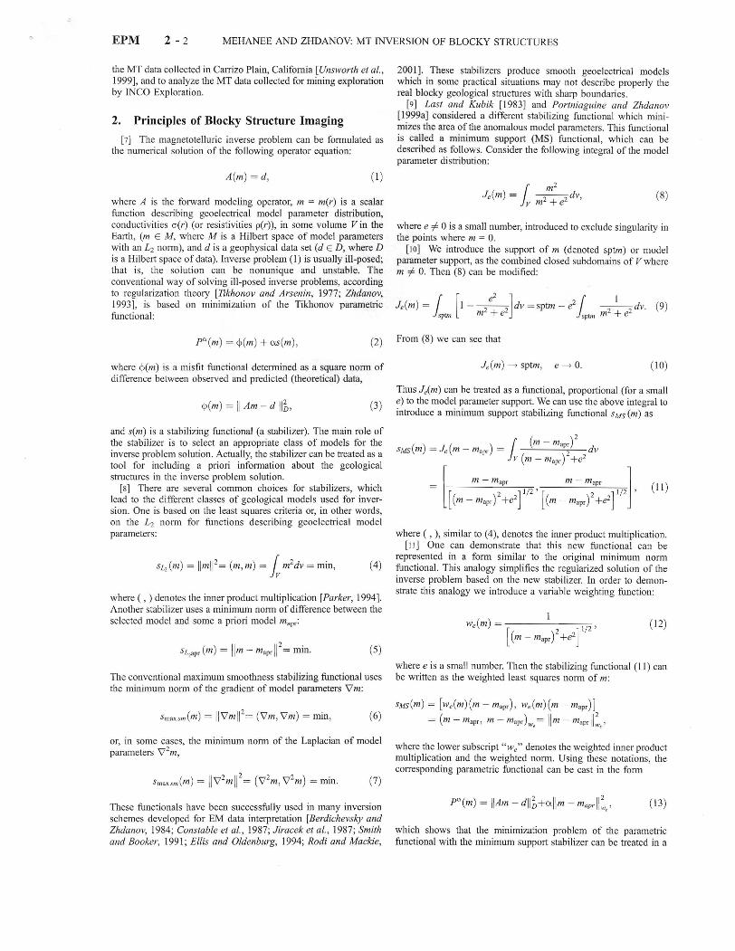
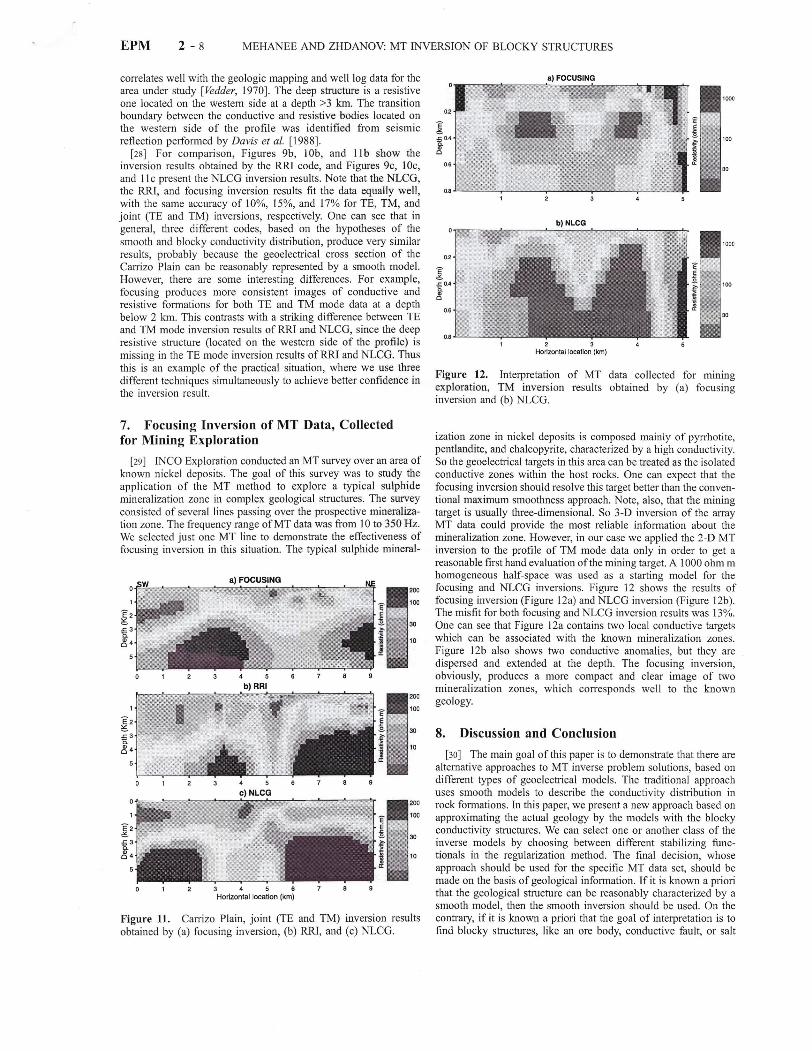
[28} For comparison, Figures 9b, lOb, and lIb show the inversion results obtained by the RRI code, and Figures 9c, 10c, and II c present the NLCG inversion results. Note that the NLCG, the RRI, and focusing inversion results fit the data equally well, with the same accuracy of 10%, 15%, and 17% for TE, TM, and joint (TE and TM) inversions, respectively. One can see that in general, three different codes, based on the hypotheses of the smooth and blocky conductivity distribution, produce very similar results, probably because the geoelectrical cross section of the Carrizo Plain can be reasonably represented by a smooth model. However, there are some interesting differences. For example, focusing produces more consistent images of conductive and resistive formations for both TE and TM mode data at a depth below 2 km. This contrasts with a striking difference between TE and TM mode inversion results of RRI and NLCG, since the deep resistive structure (located on the western side of the profile) is missing in the TE mode inversion results ofRRI and NLCG. Thus this is an example of the practical situation, where we use three different techniques simultaneously to achieve better confidence in the inversion result.

7. Focusing Inversion of MT Data, Collected for Mining Exploration

[29} INCO Exploration conducted an MT survey over an area of known nickel deposits. The goal of this survey was to study the applic ation of the MT method to explore a typica l sulphide mineralization zone in complex geological structures. The survey consisted of several lines passing over the prospective mineraliza­tion zone. The frequency range of MT data was from 10 to 350 Hz. We selected ju st one MT line to demonstrate the effectiveness of focusing inversion in this situation. The typical sulphide mineral­

~ -a: ss ,,:<

200

100

~ 2 30

~3 10~4

5

b)RRI. 200

_ _

~llr•

1lIIIiIIIIIIIII 100

~t ~·rr Jl~~ ' , ,

100

E E~2

~3

• • ;1 3'11 i i i

J!:'

~ : 10~4 ~

4 5

c) NLCG 200

~ E2

_

E ~ -"3

~4 ~ 10

3 4 5 6 Horizonta l location (km)

Figure n. Carrizo Plain, joint (TE and TM) inversion results obtained by (a) focusing inversion, (b) RRI, and (c) NLCG.

a) FOCUSING

1000

02

;[ £ 0.4 100 g­o

0.6 30

oa

1000

02

100

0.6

I !imMmlll!iillY . 7' 1i0Ii1lilifJ -,5\10_ -::: h,,_l

W"'__~_W.~ ' · "~_'_T_ V · ~._ , -" 0, 'm ',,, " 3O

oa 2 3

Horizontal location (km)

Figure 12. Interpretation of MT data collected for rnmmg exploration, TM inversion results obtained by (a) focusing inversion and (b) NLCG.

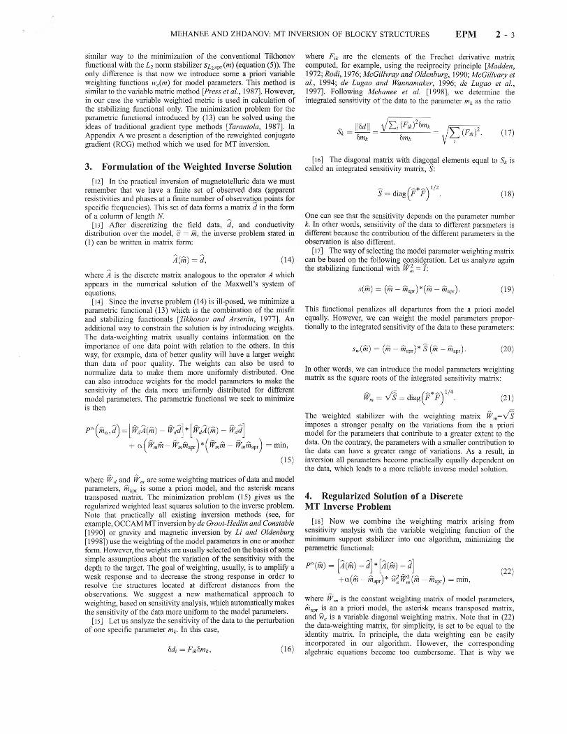
ization zone in nickel deposits is composed mainly of pyrrhotite, pentlandite, and chalcopyrite, characterized by a high conductivity. So the geoelectrical targets in this area can be treated as the isolated conductive zones within the host rocks. One can expect that the focusing inversion should resolve this target better than the conven­tional maximum smoothness approach. Note, also, that the mining target is usually three-dimensional. So 3-D inversion of the array MT data could provide the most reliable information about the mineralization zone. However, in our case we applied the 2-D MT inversion to the profile of TM mode data only in order to get a reasonable first hand evaluation of the mining target. A 1000 ohm m homogeneous half-space was used as a starting model for the focusing and NLCG inversions. Figure 12 shows the results of focusing inversion (Figure 12a) and NLCG inversion (Figure 12b). The misfit for both focusing and NLCG inversion results was 13%. One can see that Figure 12a contains two local conductive targets which can be associated with the known mineralization zones. Figure 12b also shows two conductive anomalies, but they are dispersed and extended at the depth. The focusing inversion, obviously, produces a more compact and clear image of two mineralization zones, which corresponds well to the known geology.

8. Discussion and Conclusion

[30} The main goal of this paper is to demonstrate that there are alternative approaches to MT inverse problem solutions, based on different types of geoelectrical models. The traditional approach uses smooth models to describe the conductivity distribution in rock formations. In this paper, we present a new approach based on approximating the actual geology by the models with the blocky conductivity structures. We can select one or another class of the inverse models by choosing between different stabilizing func ­tionals in the regularization method. The final decision, whose approach should be used for the specific MT data set, should be made on the basis of geological information. If it is known a priori that the geological structure can be reasonably characterized by a smooth model, then the smooth inversion should be used. On the contrary, if it is known a priori that the goal of interpretation is to find blocky structures, like an ore body, conductive fault, or salt

ii

MEHAN EE AND ZHDANOV: MT INVERSION OF BLO CKY STRUCTURES EPM 2 - 9

dome structure, then the new method developed in this paper will be more appro priate. In genera l cases, when there is not enough a priori information about the study area, the best solution would be to try both techniques and to make comparative analysis of two possible geoelectrical cross sections, using both smooth and the focus ing inversions. Each of these models will prob ably fit the data with the same accuracy. The addi tional geo logical analysis and the comparison w ith other geo physica l data on ly could make it possible to select one or another solut ion. Our code, based on focusing inversion, is designed in such a way that it can generate the minimum norm and the focused solutions simultaneously. Thi s resul t is reached by a simple se lectio n o f the correspond ing we ighting matrix Wedefi ned by (24). In the case of the minimum norm inversion this matrix is selected to be equa l to identity matrix. In the case of the focusing invers ion it is a varia ble matrix, determined by (24). The output of the code consists of two result ing models, fitting the data with the same accuracy but generating two different images. Thu s the new techniqu e presented in this paper brings more flexibility in the interpretation of MT data, leaving the final cho ice of the most suitable model to the user.

[31] We have applie d this technique for crusta l imag ing by invert ing the magnetotelluri c data acquired in the Carrizo Pla in area of Californi a. Our inversion result confirms the principal geoelectrical structures recovered in previous public ation s [Mackie et al., 1997; Unsworth et al., 1999] but also produces more focu sed and consistent images of conductive and resistive formations for both TE and TM mode data at depth below 2 km. We suggest that both images, obtained by traditional smooth inversion and by the new method, are useful for further interpre tation and analysis because they provide complimentary information about the deep geoelectr ical struc tures . Finally, application of the new focusing inversion to MT data collected for mining exploration by INCO Explora tion clearly demonstrates the adva ntage of the new tech ni­que in this situation.

Appendix A: Reweighted Conjugate Gradient (RCG) Method in the Space of Weighted Parameters

[32] The problem ofparam etric functional minimization (22) can be reform ulated in the space of weighted parameters, introd uced as

iiiW = Wm em , (A I)

where

W.ne= we Wm . (A2)

We can consider the forward operator which relates the new weighted parameters ,nw to the data

d= AW(in"'). (A3)

In order to keep the same data we should assume

WA = AW;;). (A4)

[33] Us ing these notatio ns, we can rewrit e the parametric func­tiona l (22) as

P"(mw,d) = [A ( W,~el mw) - d) *(A(W;;e1 mw) - d]

+Ci(m -w- m )*(-mw- m-w )• (AS) -r-w apr apr

In other words, we keep the same misfit, as in (22 ), because

<pw(m) = [A ( W~) mw) - d] *[A ( W,~el mw) - d]

= [A(m) - d]* [A(m)- d], (A6)

and the same stabilizer, as in (22), equa l to the least squares norm of difference (m - mapr) with the weights

Sw = (inw - ;n;pr )*(m W

- m;pr)

= (m- mapr )*W,~ e (m - mapr ) ' (A7)

[34] To construct the iterative process in the space of weig hted parameters, one can apply the conventional conjugate grad ient method [Tarantola, 1987] to find the minimum of the parametric functional (AS). However, in this case we should take into acco unt the nonl inea r character of the transformati on s (A I ) and (A2) . Portniagu ine and Zhdanov [1999, 1999 b] and Zhdano v and Hursan [2000 ] have developed a more efficient approach to the solution of this probl em, based on so-called reweighted regularized conjugate gradient (RCG) method . In the fram ewo rk of th is app roach the variable we ighting matrix We is precomputed on each iteration, We= Wen = we(mn) based on the va lues m.. obtained on the previou s iteration. As a result, the weighting matrix Wme is updated on each iteration as well,

Wme = Well w'n l (A8)

and it is treated as a fixed matrix on each iterat ion. The refore the transformations (A I) and (A2) on each iteration can be treated as linear operations, which simplifies significantly all calculations.

[35] This approach uses the idea of adaptive regularization [Zhdallov, 1993], which invo lves up dating the regularization parameter Ci on each iterat ion. The on ly difference is that we update now the regu larization parameter and the weighting matrix simultaneous ly. Note that witho ut ada ptive regulariza tion one shou ld solve the minimization prob lem for param etric functiona l (AS) many times for different values of the regularization param­eter o, which is an extremely time consuming and impractical approach. The adaptive regularization substitutes this compl icated procedure by one grad ient-type iterative process with the regula­rization parameter Ci changing from iteration to iterat ion. We use similar approach in our reweighted algorithm.

[36] The reweighted RCG method is based on the successive line search in the conjuga te gradient directi on !(mn):

-t-w <-w -r-w -r-w -(-w) mll +1 = mil + 811l = IIlIl - kill IIl n .

The idea of the line search can be described as follow s. We present P"'[m;:' - k!(m;:' )] as a function of one variable k and, evaluating it three times along direction I(mn ) , approx imately fit it by a parabola and find its minimum and the value of kn , correspondin g to this minimum .

[37] The conjugate gradient directions !(m;;') are selected with the following steps: In the first step we use the gradient direction

I(m il ) = I(mil ) = W~) F* [A(W,~el mil) - d]+ Ci(mil - m;;'r) . (A9)

In the next step, the conjuga te gradient direction is the linear combination of the gradient in this step and the direct ion I(mo)in the

EPM 2 - 10 MEHANEE AND ZHDANOV: MT rNVERSION OF BLOCKY STRUCTURES

previous step:

7(mn = 7(m7) + ~ 1 7(m~) .

In the nth step,

7(m:+1) = 7(m:+1) + ~1l+ J (m:),

where

17(m:) = v:F*[.4 (W';;-em:) - d] + a(m: - m;p} (AIO)

[38] The coefficients ~ 'L+ l are defined from the condition that the directions [(mn+l) and [(mil) are conjugate:

2

117(m:+1) 11(A l l)~ Il+ l = 2 .

1 1 7(m~ ) II

In the last step we recompute the real parameters of the model from the weighted parameters at the nth iteration:

mfl+l = W';e1m:+l = W:;;-elw~/ m:+l' (AI2)

[39] The regularization parameter a describes the trade-off between the best fitting and most reasonable stabilization. In a case when a is selected to be too small, the minimization of the parametric functional P"(m) is equivalent to the minimization of the misfit functional <Pw(m); therefore we have no regularization, which can result in an unstable incorrect solution. When a is too large, the minimization of the parametric functional F(m) is equivalent to the minimization of the stabilizing functional sw(m), which will force the solution to be closer to the a priori model. Ultimately, we would expect the final model to be exactly like the a priori model, while the observed data are totally ignored in the inversion. Thus the critical question in the regularized solution of the inverse problem is the selection of the optimal regularization parameter a. The basic principles used for determining the regularization parameter a are discussed by Tikhonov and Arsenin [1977] and Zhdan ov [1993]. It can be selected from the progression of numbers

ak =aOq\ k=0,1 ,2, . . . , n; q >O. (Al3)

For any number ak we can find an element mo.., minimizing P'" (m), and calculate the misfit 11.4(mo.. - df The optimal value of the parameter a is the number akO, for which we have

2 11.4(m"kO )- dl1= 52, (A I4)

where 5 is the level of noise in the observed data. The equality (AI4) is called the misfit condition.

[40] In our code, as we have mentioned above, we use the adaptive RCG method [Zhdanov, 1993]. In the framework of this method we begin an iteration from a value of ao, which can be obtained as a ratio of the misfit functional and stabilizer for an initial model, then reduce all according to (Al3) on each subse­quent iteration and continuously iterate until the misfit condition (A14) is reached.

[41] Note that on each iteration of the reweighted RCG method we actually minimize the parametric functional with the different stabilizers because the regularization parameter and the weighting

matrix Wen are updated on each iteration. In order to insure the convergence of the misfit functional to the minimum we check the misfit value on each iteration . We decrease the regularization parameter a if the misfit does not decrease fast enough. This procedure in combination with the parabolic line search in the conjugate gradient direction on every iteration insures the con­vergence of the method.

[42] Acknowledgments. The MT data from the Carrizo Plain were collected with financial support from the USGS under grant 1434-94-6­2423 and from the National Science Foundation under grant EAR 9316160. We are thankful to the University of Washington and, in particular, to Martin Unsworth and Gary Egbert for providing the MT data. We are thankful, also, to INCO Exploration and, in particular, to Alan King and Steve Balch for providing MT data, collected for mining exploration, and permission to publish the inversion results. The authors acknowledge the support of the University of Utah Consortium for Electromagnetic Model­ing and Inversion (CEMI), which includes Advanced Power Technologies Inc., AGIP, Baker Atlas Logging Services, BHP Minerals , EXXON­MOBIL Upstream Research Company, INCO Exploration, Japan National Oil Corporation , MINDECO, Naval Research Laboratory, Rio Tinto-Ken­necott, 3JTech Corporation, and Zonge Engineering. We are thankful to anonymous reviewers for their useful comments and recommendations, which helped to improve the manuscript.

References Berdichevsky, M. N., and M. S. Zhdanov, Adva nced Theory of Deep

Geomagnetic Sounding, 408 pp., Elsevier Sci., New York, 1984. Constable, S. C., R. C. Parker, and G. G. Constab le, Occam's inversion:

A practical algorithm for generating smooth models from EM sounding data, Geophysics, 52, 289- 300, 1987.

Davis, T. L., M. B. Lagoe, W. J. M. Bazeley, S. Gordon, K. McIntosh, and J. S. Namson, Structure of the Cuyama Valley, Caliente Range and Carrizo Plain and its significance to the structural style of the southern Coast Ranges and western Transverse Ranges, in Tertiary Tectonics and Sedimentation ofthe Cuyama Basin. San Luis Obispo, Santa Barbara and Ventura Counties, California, edited by W. J. M. Bazeley, pp. 141- 158, Pac. Sect., Soc. of Econ. and Paleoentol. Mineral., Bakersfield, Calif., 1988.

de Groot-Hedlin, C. D., and S. C. Constable, Occam 's inversion to generate smooth, two-dimensional models from magnetote lluric data, Geophysics, 93, 1613-1624, 1990.

de Lugao, P., and P. E. Wannamaker, Calculating the two-dimensional magnetotelluric Jacobian in finite elements using reciprocity, Geophys. J Int., 127, 806-810, 1996.

de Lugao, P., O. Portniaguine, and M. S. Zhdanov, Fast and stable two­dimensional inversion of magnetotelluric data, J. Geomagn. Geoelectr., 49, 1469- 1497, 1997.

Ellis, R. G., and D. W.Oldenburg, The pole-pole 3-D DC-resistivity inverse problem: A conjugate gradient approach, Geophys. J lnt., 119, 187-1 94, 1994.

Graff, L. B., Exploration drilling in the Carrizo Plain, in Guidebook to the Geology of Carrizo Plain and San Andreas Fault , pp. 21- 24, San Joaquin Geol. Soc., 1962.

Hoversten, G. M., H. F. Morrison, and S. C. Constable, Marine magneto­tellurics for petroleum exploration, part Il, Numerical analysis of subsalt resolution, Geophysics, 63, 826-840, 1998.

Jiracek, G. R., W. L. Rodi, and L. L. Vanyan, Implications of magnetotel­luric modeling for the deep crustal environment in the Rio Grande Rift, Phys. Earth Planet. Inter., 45, 179-1 92,1 987.

Last, B. J., lind K. Kubik, Compact gravity inversion , Geop hysics, 48, 713- 72 1,1 983.

Li, Y., and D. W. Oldenburg, 3-D inversion of gravity data, Geophysics, 63, 109-11 9, 1998.

Mackie, R. L., D. W. Livel ybrook s, T. R. Madden , and J. C. Larsen, A magnetotelluric investigation of the San Andreas Fault at Carrizo Plain, California, Geophys. Res. Lett., 24, 1847- 1850, 1997.

Madden, T. R., Transmission system and network analogies to geophysical forward and inverse problems, Rep. 72-3, Dep. of Earth and Planet. Sci., Mass. Inst. of Technol., Cambridge, 1972.

McGillvray, P. R., and D. W. Oldenburg, Methods for calculating Frechet derivatives and sensitivities for the non-linear inverse problem: A com­parative study, Geophys. Prospect., 38, 499- 524, 1990.

McGillvary, P. R., D. W. Oldenburg, R. G. Ellis, and T. M. Habashy, Calculation of sensitivities for the frequency domain electromagnetic problem, Geophys. J. Int., 116, 1-4, 1994.

Mehanee, S., N. Golubev, and M. S. Zhdanov, Weighted regularized in­

MEHANEE AND ZHDANOV: MT INVERSION OF BLOCKY STRUCTURES EPM 2 - 11

version of magnetotelluric data, paper presented at International Exposi­tion and Meeting, Soc. of Expl. Geophys ., New Orleans, La., 13- 18 Sept. 1998.

Page, B. M., The southe m Coas t Ranges, in The Geotectonic Development of California, edited by W. G. Ernst, pp. 329 -41 6, Prentice-Hall, Old Tappan, N. J., 1981.

Parker, R. L., Geophysical Inverse Theory, 386 pp., Princton Univ. Press, Princeton, N. J., 1994.

Port niaguine, 0 ., and M. S. Zhdanov, Focusing geophysical inversion images, Geophysics, 64, 874 - 887, 1999a.

Portniaguine, 0 ., and M. S. Zhdanov, 3-D focusing inversion of CSMT data, in Three-Dimensional Electromagnetics, Proceedings ofthe Second International Symposium, pp. 132-1 35, Univ. of Utah, Salt Lake City, 1999b.

Press, W. H., B. P. Flannery, S. A. Teukolsky, and W. T. Veterling, Numer­ical Recipes: The Art ofScientific Computing, 818 pp., Cambridge Univ. Press, New York, 1987.

Rodi, W. L., A techn ique for improving the accuracy of finite elemen t solutions for magnetotelluric data, Geophys. J. R. Astron. Soc., 44, 483 -506, 1976.

Rodi, W. L., and R. L. Mackie, Nonlinear conjugate gradients algorithm for 2-D magnetotelluric inversion, Geophysics, 66, 174-187,2001.

Simonson, R. R., Crocker Flat landslide, Recruit Pass area, in Guidebook to the Geology of Carrizo Plain and San Andreas Fault, pp. 14- 15, San Joaquin Geol. Soc., 1962.

Smith, J. T., and J. R. Booker, Rapid inversion of two- and three-dimen­sional magnetotelluric data, J. Geophys. Res., 96, 3905 -3922, 1991.

Tarantola, A., Inverse Problem Theory, 613 pp., Elsevier Sci., New York, 1987.

Tikhonov, A. N., and V. Y. Arsenin, Solutions of Ill-posed Problems, 258 pp., John Wiley, New York, 1977.

Unswo rth, M. J., G. D. Egebert, and J . R. Booker, High resolution electromagnetic imaging of the San Andreas Fault in centra l Califor­nia, J. Geophys. Res., 104, 1131- 1150, 1999.

Vedder, J. G., Geologic map of the Wells Ranch and Elkhorn Hills quad ­rangles, San Luis Obispo and Kern Counties, California, Us. Geol. Surv Misc. Geol. Invest. Map, 1-585, 1970.

Zhdanov, M. S., Tutorial: Regularization in Inversion Theory, Colo. Sch. of Mines" Golden, 1993.

Zhdanov, M. S., and G. Hursan, 3D electromagnet ic inversion based on quasi-analytical approximation, Inverse Problems, 16, 1- 26, 2000.

Zhdanov, M. S., N. G. Golubev, V. V. Spichak, and I. M. Varentsov, The construction ofeffective methods for electromagnetic modeling , Geophys . J. R. Astron. Soc., 68, 589 -607, 1982.

S. Mehanee and M. Zhdanov, Department of Geology and Geophysics, University of Utah, 135 South 1460 East, RM 719, Salt Lake City, UT 84112-0111, USA. (smehanee@mines.utah.ed u; mzhdanov@mines.utah. edu)