TWO DIMENSIONAL PARTICLE FLOW INSIDE DRIVEN TRAPEZOID APPLYING EULARIAN-LAGRANGIAN APPROACH NOR HAFRIZ BINTI ABD HALIL A report submitted in partial fulfillment of The requirements for the award of the degree of Bachelor of Mechanical Engineering Faculty of Mechanical Engineering UNIVERSITI MALAYSIA PAHANG JUNE 2013
Transcript
TWO DIMENSIONAL PARTICLE FLOW INSIDE DRIVEN TRAPEZOID
APPLYING EULARIAN-LAGRANGIAN APPROACH
NOR HAFRIZ BINTI ABD HALIL
A report submitted in partial fulfillment of
The requirements for the award of the degree of
Bachelor of Mechanical Engineering
Faculty of Mechanical Engineering
UNIVERSITI MALAYSIA PAHANG
JUNE 2013
vii
ABSTRACT
In this report, Navier Stokes Equation (NSE) method is use to simulate lid-
driven flow in a two dimensional isosceles trapezoidal cavity. For the first part in this
report, the simulation of the NSE are compared with the existing research (Lattice
Boltmann Method of lid-driven flow in trapezoidal cavities) and for the second part is to
studied about the number of the vortexes based of Reynolds numbers. For these
numerical simulations, the effect of Reynolds numbers, various lid movement and
number of vortices in the isosceles trapezoidal cavities are studied. Re is varied from
100 to 7500. Numerical result show that, as the Re increases, the phenomena in the
cavity becomes more and more complex, and the number of the vortexes increases.
Furthermore, as Re is increased, the flow in the cavity undergoes a complex transition
(from steady to the periodic flow and finally to the chaotic flow). For the various lid
movements, the maximum number of the vortexes is six when upper and the bottom lid
move in the same direction.
viii
ABSTRAK
Dalam laporan ini, kaedah Persamaan Navier Stokes (NSE) adalah digunakan
untuk mensimulasikan aliran didorong tudung dalam dimensi rongga sama kaki
trapezoid dua. Untuk bahagian pertama di dalam laporan ini, simulasi NSE
dibandingkan dengan penyelidikan yang sedia ada (Lattice Boltmann Kaedah aliran
didorong tudung dalam rongga trapezoid) dan bahagian kedua adalah untuk mengkaji
tentang bilangan putaran berdasarkan nombor Reynolds . Untuk simulasi berangka ini,
kesan nombor Reynolds, pelbagai pergerakan tudung dan bilangan vorteks dalam
rongga trapezoid sama kaki dikaji. Re diubah 100-7500. Menunjukkan hasil berangka
bahawa, sebagai Re bertambah, fenomena dalam rongga menjadi lebih dan lebih
kompleks, dan bilangan putaran bertambah. Tambahan pula, sebagai Re meningkat,
aliran dalam rongga menjalani peralihan kompleks (daripada stabil kepada aliran
berkala dan akhirnya aliran huru-hara). Untuk pelbagai pergerakan tudung, bilangan
maksimum putaran adalah enam apabila atas dan tudung langkah bawah dalam arah
yang sama.
ix
TABLE OF CONTENTS
TITLE PAGE I
EXAMINER DECLARATION II
SUPERVISOR DECLARATION III
STUDENT DECLARATION IV
ACKNOWLEDGEMENT VI
ABSTRACT VII
TABLE OF CONTENTS IX
LIST OF FIGURES XII
LIST OF TABLE XIII
CHAPTER
1
INTRODUCTION
1.0 INTRODUCTION 1
1.1 PROJECT BACKGROUND 1
1.2 PROBLEM STATEMENT 1
1.3 OBJECTIVES 2
1.4 SCOPE OF STUDY 2
1.5 INTRODUCTION TO NAVIER STOKES
EQUATION 2
1.6 STRUCTURE OF REPORT 3
CHAPTER
2
LITERATURE REVIEW
2.0 INTRODUCTION 4
2.1 FLOW BEHAVIOUR IN LID DRIVEN
CAVITY
4
2.2 DRIVEN CAVITY 5
x
2.3 EULERIAN-LAGRANGIAN 8
2.4 REYNOLDS NUMBERS 11
2.5 NAVIER-STOKES EQUATION 13
2.6 CONTINUITY EQUATION 14
2.7 STREAM FUNCTION-VORTICITY
NAVIER-STOKES EQUATION
17
2.8 GOVERNING EQUATIONS IN CAVITY
FLOW
17
2.9 PRIMITIVE VARIABLES VERSUS
STREAM FUNCTION-V0RTICITY
APPROACH
18
2.10 DIMENSIONLESS VARIABLES 21
2.11 DISCRETIZATION 22
CHAPTER
3
METHODOLOGY
3.0 INTRODUCTION 24
3.1 BOUNDARY CONDITION 24
3.2 METHODOLOGY FLOW CHART 28
3.3 COLLECT INFORMATION 30
3.4 STUDY EXISTING CODE 30
3.5 RUN EXISTING CODE 32
3.6 MODIFY CODING 33
3.7 ADD NEW TERM
( BOUNDARY LIMITS AND SHAPE )
34
3.8 RUN THE SIMULATIONS 36
xi
3.9 CHAPTER SUMMARY 36
CHAPTER
4
RESULT AND DISCUSSION
4.1 INTRODUCTION 37
4.2 LID-DRIVEN CAVITY FLOW 37
4.3 COMPARISON OF RESULT FOR FD-NSE
AND LBM 39
4.3.1 Result (physical) 39
4.3.2 Result (data) 42
4.4 RESULT WITH VARIOUS VALUE OF
REYNOLDS NUMBERS FOR DIFFERENT
DIRECTION AND POSITION OF
VELOCITY
44
4.4.1 44
4.4.2 48
4.4.3 52
4.4.4 56
4.4.5 60
4.4.6 65
CHAPTER
5
CONCLUSSION AND
RECOMENDATION
5.1 CONCLUSSION 69
5.2 RECOMENDATION 70
REFERENCES 71
APPENDICES A-D 73
xii
LIST OF TABLE
Table Title No. Of
page
Table 4.1 First, second and third primary eddies characteristics at
different Reynolds numbers for NSE
42
Table 4.2 First, second and third primary eddies characteristics at
different Reynolds numbers for LBM
43
Table 4.3 Percentage of error for the comparison position of 1st, 2
nd
and 3rd
eddies at different Reynolds number
43
Table 4.4 First, second and third primary eddies characteristics for
different Reynolds numbers at
45
Table 4.5 First, second and third primary eddies characteristics for
different Reynolds numbers at
49
Table 4.6 First, second, third, fourth and fifth primary eddies
characteristics for different Reynolds numbers at
53
Table 4.7 First, second, third, fourth and fifth primary eddies
characteristics for different Reynolds numbers at
57
Table 4.8 First, second and third primary eddies characteristics for
different Reynolds numbers at
61
Table 4.9 Fourth, fifth and sixth primary eddies characteristics for
different Reynolds numbers at
61
Table 4.10 First, second and third primary eddies characteristics for
different Reynolds numbers at
66
xiii
LIST OF FIGURES
Figure Title Page
Figure 2.1 Coordinate of the isosceles trapezoidal cavity 5
Figure 2.2 The schematic diagram for 2D lid-driven cavity 6
Figure 2.3 Lagrangian of particle flow 9
Figure 2.4 Eularian description of fluid flow 10
Figure 2.5 Schematic view of driven cavity flow for square 13
Figure 2.6 The coquette flow at the steady state 15
Figure 2.7 Numerical and analytical graph of coquette flow 16
Figure 3.1 Boundary condition of a Lid-driven cavity flow 24
Figure 3.2 The boundary for a 2D lid driven cavity 25
Figure 3.3 Methodology flow chart 29
Figure 3.4 Streamline plot of square cavity flow with different
Reynolds number which is 100, and 1000
33
Figure 3.5 Modify coding ( Where change size of grid) 33
Figure 3.6 Modify coding
(Where change the boundary nodes of the vorticity and
which part moving)
34
Figure 3.7 Meshing in Two Dimension 34
Figure 3.8 Flow chart for NSE 35
Figure 4.1 The schematics diagram for 2D lid driven cavity 38
Figure 4.2 The boundary for a 2D lid driven cavity 38
Figure 4.3 Streamline plot using NSE method for Reynolds number
100,1000, 3200, 5000 and 7500.
39
Figure 4.4 Streamline plot using LBM for Reynolds number
100,1000, 3200, 5000 and 7500.
40
Figure 4.5 Streamline plot of , for Reynolds number
100,1000,3200,5000 and 7500
44
Figure 4.6 Variation of the X₁ and Y₁ direction coordinates of the
central location with Re
46
Figure 4.7 Velocity profile at the with the vertical position
for variation of Reynolds number
46
Figure 4.8 Streamline plot of , for Reynolds number
100,1000,3200,5000 and 7500
48
Figure 4.9 Variation of the X₁ and Y₁ direction coordinates of the
central location with Re
50
Figure 4.10 Velocity profile at the with the vertical position
for variation of Reynolds number
50
Figure 4.11 Streamline plot of , for Reynolds number
100, 1000, 3200, 5000 and 7500.
52
Figure 4.12 Variation of the X₁ and Y₁ direction coordinates of the
central location with Re
54
Figure 4.13 Velocity profile at the with the vertical position
for variation of Reynolds number
54
xiv
Figure 4.14 Streamline plot of , for Reynolds number
100,1000,3200,5000 and 7500
56
Figure 4.15 Variation of the X₁ and Y₁ direction coordinates of the
central location with Re
58
Figure 4.16 Velocity profile at the with the vertical position
for variation of Reynolds number
58
Figure 4.17 Streamline plot of , for Reynolds
number 100, 1000, 3200,5000 and 7500
60
Figure 4.18 Variation of the X₁ and Y₁ direction coordinates of the
central location with Re
63
Figure 4.19 Velocity profile at the with the vertical position
for variation of Reynolds number
63
Figure 4.20 Streamline plot of , for
Reynolds number 100, 1000, 3200,5000 and 7500
65
Figure 4.21 Variation of the X₁ and Y₁ direction coordinates of the
central location with Re
67
Figure 4.22 Velocity profile at the with the vertical position
for variation of Reynolds number
67
xv
LIST OF ABBREVIATIONS
E-L Eularian- Lagrangian
NSE Navier-Stokes Equation
LBM Lattice Boltzmann Method
CFD Computational Fluid Dynamics
FDM Finite Element Method
FVM Finite Volume Method
CIP Cubic Interpolated Pseudo-Particle
xvi
LIST OF SYMBOLS
AR Aspect Ratio
H Height of cavity
P Pressure
ρ Density
Re Reynolds Number
T Time
T Dimensionless time
U Velocity in x direction
Lid velocity
U Dimensionless velocity in x direction
V Velocity in y direction
V Dimensionless velocity in y direction
Kinematic Viscosity
W Width of the cavity
X Axial distance
X Dimensionless axial distance
Y Vertical distance
Y Dimensionless vertical distance
Μ Dynamics viscosity
Kinematic viscosity
Ω Vorticity
Ω Dimensionless vortocity
Ψ Stream function
Ψ Dimensionless stream function
L Length
xvii
Superscript
N Current Value
n+1 Next step value
* Non advection phase value
Subscript
I x direction node
J y direction node
max i x direction maximum node
Max j y direction maximum node
,e Free stream condition
xviii
LIST OF APPENDICES
A Gantt chart 73
B Codes for cavity flow of Trapezoidal 74
C Codes of Streamline 80
D Codes of velocity 82
CHAPTER 1
INTRODUCTION
1.1 PROJECT BACKGROUND
The main idea of this project is to expose student with many aspect of
engineering work; run simulation using MATLAB, edit existing coding, about the
particle flow and the effect of Reynolds Number and particle position. The task follows
a common product development activity, where student need to apply all their
engineering knowledge and skill to complete this project. In random, student must know
some basic knowledge which is definition of particle flow, software and about the
experiment. In the other hand, student must master in conceptual of modifying code and
run the coding using MATLAB. Not only that, student must know how to solve
problem in edit the coding.
1.2 PROBLEM STATEMENT
Pattern of the particle flow will change if Reynolds number and particle position not
fixed. What will happen to the pattern of the particle flow when it is at different
Reynolds number and various lid movements.
2
1.3 OBJECTIVES
Objectives of this project are:
- To identify flow inside driven trapezoid cavity for different Reynolds number.
- To study the vortex structures of flow for various lid movements.
1.4 SCOPE OF THE STUDY
Scopes for this particular research are bounded by these three matters and therefore
will be followed throughout the research :
- Applying Eularian – Langrangian approach
- Study on the vortex structures of flow with various lid movements.
( , ).
- Focus on different Reynolds numbers.
(100, 1000, 3200, 5000, 7500)
- Do simulation on the vortex structures of flow with different Reynolds number
and various lid movements using Matlab.
1.5 INTRODUCTION TO NAVIER STOKES EQUATION
Navier-Stokes equation is well known in the field of fluid dynamic. The
equation is nonlinear and usually the flows that apply this equation are considered
incompressible. Many fluid flows are governed by this equation because in describing
the conservation of momentum, the equation is almost perfect. The equation consists the
unsteady term, the diffusive term, pressure term, convective term and the external force.
In spite, there is no analytical solution to this equation as there are many Partial
differential terms in the equation.
3
1.6 STRUCTURE OF REPORT
This report consists of five chapters which are Chapter 1 (introduction), chapter
2 (literature review), chapter 3 (methodology), chapter 4 (result and discussion) and
chapter 5 (conclusion). Chapter 1 is focused on the basic information about the study
which is background of study, problem statement, objectives of study, scope and the
structure of this project.
While chapter 2 was focused on the review of past studies that are relate to this
study. This chapter includes about particle flow, driven cavity, Lagrangian-Eularian,
Reynolds Numbers and some equations that related to this topic. A review of other
relevant research studies also provided. The review is detailed so that the present
research effort can be properly tailored to add to the present body of literature as well as
to justly the scope and direction of the present research effort.
In chapter 3, a review of the methodology that has been suggested in conducting
the study was provided. It is start with the designing of the study, what the activities in
performing this study has been reviewed. This chapter reviews the planning that has
been suggested in conducting the study. A review of data analysis and software that will
be used also discussed in general.
Chapter 4 was focused on collecting data from the simulation. The data focus on
pattern of particle flow for different Reynolds number and various lid movements that
had been used. The data will be used to make analysis. The data has been analyzed
using graphs and table. This chapter also provided a discussion for data and analysis of
the results.
Finally, chapter 5 was conclusion of this project and discusses some
recommendations for futurer work.
CHAPTER 2
LITERATURE REVIEW
2.0 INTRODUCTION
Chapter 2 explains about literature review of the project. All the theories,
concepts, and other related standards that related to the study were reviewed. It includes
particle flow, Reynolds number, and method that use. A review of other relevant
research studies also provided.
2.1 FLOW BEHAVIOUR IN LID DRIVEN CAVITY
In many industrial processes, including the transport of solids in liquids and
removal of particulates from gas streams for pollution control, particle flow is most
important things. The main problems of flow in industrial design involve the flow of
liquids or gas with suspended solids.
Stokes number is a key parameter in fluid-particle flows, which is the ratio of
the response time of a particle to a time characteristic of a flow system. The time that a
particle takes to respond to a change in carrier flow velocity is known as a particle
response time. The Stokes number is small when it is less than 0.1, then the particles
have sufficient time to respond to the change in fluid velocity, so the particle velocity
approaches the fluid velocity. However, if the Stokes number is large where is greater
than 10, the particles have short time to respond to the varying fluid velocity and the
particle velocity shows little change.
5
O
H
L
The relative concentration of the particles in the fluid is referred as the loading.
There are several ways to define the loading, such as the ratio of particle mass flow to
fluid mass flow. Highly loaded particle flows were involved in many industrial
applications.
When the particle loading is small, the fluid will affect the particle properties,
such as velocity and temperature and the fluid properties will not be influenced by the
particle. This is referred to as one-way coupling. If the condition is that there is a mutual
interaction between the particles and fluid, the flow is two-way-coupled. When the
Stokes number increasing, the two-way coupling effect will reduce because the particles
undergo acceleration.
The flow is termed dilute if the particles motion is controlled by the action of the
fluid on the particle. The particles will collide with each other and their motion will be
depending on particle-particle collisions, when the particle concentration is sufficiently
high and the flow is then regarded as dense.
2.2 DRIVEN CAVITY
Figure 2.1 Coordinate of the isosceles trapezoidal cavity
In this section, the trapezoidal cavity model is first introduced. L is the length of
the top wall and H is the height of the cavity. In all simulations presented here. L and H
are set to be 1 and 0.577.
6
A
B C
D
Figure 2.2 The schematic diagram for a 2D lid driven cavity
The flow in the driven cavity will be divided into two groups it the development
of new numerical schemes (where the driven cavity is used as a benchmark) and is the
analysis of the physics of the flow it is stated in most of the paper. For these objectives,
there are a lot of works devoted to the issue of transition to turbulence and regarding to
the location of the so-called first Hopf bifurcation.
A few work has been done on rectangular rather than square cavities. Some of
researchers used a lattice boltzmann method for the analysis of the 2D vortex structure
in a rectangular lid driven cavity for the various Reynolds numbers and for different
depth to width ratios. There are some works devoted to the issue of motion of two walls
in the cavity rather than one wall. This is an example of the work that been done by
some researchers, where the linear stability of two counter-rotating vortices driven by
the parallel motion of the two walls is investigated by a FVM. The driven cavity will be
effect by the flow temperature, where it also been the subject of some interests, a
temperature gradient is introduced and this leads to buoyancy driven flow. The field
becomes coupled by temperature distributions and velocity.
The particles are treated as points, where motion is the result of the influence of
the fluid phase and the flow of the particles were modelled by the Eularian-Lagrangian
(E-L) approach. The biggest drawback of this method is the fact that in the real
industrial applications the number of the particles is too large to consider the behaviour
all of them.
Y
X
v u
7
In order to overcome this problem, a number of particles are often “pooled” to
form “virtual particles” with the same parameters, so that the number of the particles to
be considered can be reduced. The E–L type of model can be used accurately without
introducing virtual particles for small geometries with limited number of particles. The
E–L approach makes it possible to investigate the fundamental processes. (Elsevier
B.V.2008)
The lid driven cavity flow is most probably one of the most studied fluid
problems in computational fluid dynamics field. The easiness of the geometry of the
cavity flow makes the problem easy to code and apply boundary conditions. Sometimes
the problem looks like simple in many ways, but the flow in a cavity keeps all the flow
physics with counter rotating vortices appear at the corners of the cavity. Driven cavity
flow is the benchmark of the problem for the numerical methods in term of accuracy
and numerical efficiency. In basically the driven cavity flow can be grouped into three
categories.
For the first category studies that present steady solution is at the high Reynolds
numbers, at the presented solutions of steady 2-D incompressible flow in a driven cavity
for Re ≤ 10000. Solutions for Re=12,500 also have presented among these researchers.
Moreover, other researchers also have presented steady solutions up to Re=20,000. In
the second category, the following two dimensional Direct Numerical Simulation
studies on driven cavity flow. For the third category studies, Fortin, Gervais(2000),
Sahin(1998) and Abouhamza(2002) are examples of two dimensional hydrodynamic
stability studies on driven cavity flow.
Even though that driven cavity flow is studied at this scope in numerical studies,
the nature of the flow at high Reynolds number is still not agreed upon. For example
many studies come from the first category, where present steady solutions at very high
Reynolds numbers showing that there exists a solution for steady 2-D Navier-Stokes
equations for the flow inside the driven cavity.
8
On the other hand, after a two dimensional hydrodynamic stability analysis or Direct
Numerical Simulation, the studies from the second and third categories will claim
beyond a moderate Reynolds number. The flow in a 2-D driven cavity is unsteady,
therefore a steady solution does not exist hence a steady solution at high Reynolds
numbers is not computable.
The main purpose of this study is then to discuss the incompressible flow in a 2-
D driven cavity in terms of physical, numerical aspects and mathematical, together with
a very brief literature survey on numerical studies and experimental. We will also
present very fine grid steady solutions for the driven cavity flow at very high Reynolds
numbers. We will discuss on the driven cavity flow in an attempt to address the
important points mentioned as above. (Ercan Erturk,2009)
2.3 EULERIAN-LAGRANGIAN
Normally Eulerian-Lagrangian approach is widely used to simulate dispersed
two-phase of the flows. In this approach the dispersed phase is represented by discrete
particle in a Lagrangian frame, while the carrier phase is represented by continuous
field in an Eulerian frame reference. The mean interphase momentum transfer term
cannot be neglected, and two-way coupling effects must be accounted for when it occur
in two-phase flows with non-negligible mass loading. The mean interphase momentum
transfer term, it is the average force of exerted by the particles on the fluid and accounts
for the presence of the dispersed phase on the fluid phase.
In numerical implementations of the Eulerian-Lagrangian method, the numerical
estimate of the mean interphase momentum transfer term (or any other mean quantity)
at Eulerian grid nodes is obtained using a finite number of particles, leading to statistical
and bias errors (Garg et al,2007).
Statistical error can be reduced either by increasing the number of particles, or
by averaging over multiple independent realizations. Bias error is insensitive to the
number of independent realizations and becomes zero only in the limit of infinite
particles or also called the dense data limit.
9
In addition to these errors, a finite time is a main step to the usual spatial and a
finite number of grid cells and temporal discretization errors that are encountered in
numerical simulations of single-phase flow. The scaling of each of these error
contributions was bias, statistical, and discretization error.
It will divided with variation of numerical parameters determines the numerical
convergence characteristics of any Lagrangian-Eulerian numerical implementation.
Although Lagrangian-Eulerian simulations are frequently used to simulate multiphase
of flows, their numerical convergence and accuracy properties have not been critically
examined until recently.(R.Garg et al, 2008)
A fluid flow (both liquid and air) may be described in two different ways it is
the Lagrangian approach (named after the French mathematician Joseph Louis
Lagrange), and the Eulerian approach (named after Leonhard Euler, a famous Swiss
mathematician). In the Lagrangian approach, one particle is chosen and is followed as it
moves through space with time. The line traced out by that one particle is called a
particle pathline. An example is a transmitting ocean buoy that observes a set path over
regular intervals over a period of time. The path observed is the particle pathline.
Figure 2.3 Lagrangian description of Particle Flow
In the Lagrangian description of fluid flow, individual fluid particles are
"marked," and their positions, velocities are described as a function of time. In the
example shown, particles A and B have been identified. Position vectors and velocity
vectors are shown at one instant of time for each of these marked particles.
10
As the particles move in the flow field, their positions and velocities change
with time, as seen in the diagram. The physical laws, such as Newton's laws and
conservation of mass and energy, apply directly to each particle.
If there were only a few particles to consider, as in a high school physics
experiment with billiard balls, the Lagrangian description would be desirable. However,
fluid flow is a continuum phenomenon, at least down to the molecular level. It is not
possible to track each "particle" in a complex flow field. Thus, the Lagrangian
description is rarely used in fluid mechanics. A Eulerian approach is used to obtain a
clearer idea of the airflow at one particular instant. One can look at a “photograph” of
the flow of, for instance, surface ocean currents at a particular fixed time. The entire
flow field is easily visualized. The lines comprising this flow field are called
streamlines.
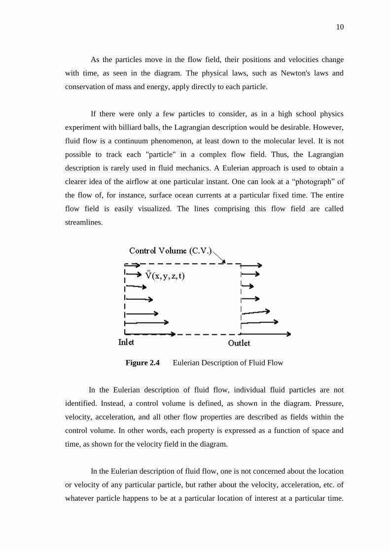
Figure 2.4 Eulerian Description of Fluid Flow
In the Eulerian description of fluid flow, individual fluid particles are not
identified. Instead, a control volume is defined, as shown in the diagram. Pressure,
velocity, acceleration, and all other flow properties are described as fields within the
control volume. In other words, each property is expressed as a function of space and
time, as shown for the velocity field in the diagram.
In the Eulerian description of fluid flow, one is not concerned about the location
or velocity of any particular particle, but rather about the velocity, acceleration, etc. of
whatever particle happens to be at a particular location of interest at a particular time.
11
Since fluid flow is a continuum phenomenon, at least down to the molecular level, the
Eulerian description is usually preferred in fluid mechanics. Note that, the physical laws
such as Newton's laws and the laws of conservation of mass and energy apply directly
to particles in a Lagrangian description. Hence, some translation or reformulation of
these laws is required for use with an Eulerian description.
2.4 REYNOLDS NUMBERS
Reynolds number can be defined for a number of different situations where a
fluid is in relative motion to a surface. These definitions generally include the fluid
properties of density and viscosity, plus a velocity and a characteristic length or
characteristic dimension. This dimension is a matter of convention – for example a
radius or diameters are equally valid for spheres or circles, but one is chosen by
convention. For aircraft or ships, the length or width can be used. For flow in a pipe or a
sphere moving in a fluid the internal diameter is generally used today.
Other shapes such as rectangular pipes or non-spherical objects have
an equivalent diameter defined. For fluids of variable density such as compressible
gases or fluids of variable viscosity such as non-Newtonian fluids, special rules apply.
The velocity may also be a matter of convention in some circumstances, notably stirred
vessels. The inertial forces, which characterize how much a particular fluid resists any
change in motion are not to be confused with inertial forces defined in the classical way.
The Reynolds number (Re) is a dimensionless number that gives a measure of
the ratio of inertial forces to viscous forces and consequently quantifies the relative
importance of these two types of forces for given flow conditions.