Two-fluid modeling of three-dimensional cylindrical gas–solidfluidized beds using the kinetic theory of granular flow

Vikrant Verma, Niels G. Deen n, Johan T. Padding, J.A.M. KuipersDepartment of Chemical Engineering and Chemistry, Eindhoven University of Technology, PO Box 513, 5600 MB Eindhoven, The Netherlands

H I G H L I G H T S

� We present a highly efficient numer-ical model for large scale densefluidized beds.

� We present a solution for the bound-ary condition at the centerline of thecylindrical grid.

� We quantify the effects of grid size,flux limiters, frictional model andcoefficient of restitution.

G R A P H I C A L A B S T R A C T

a r t i c l e i n f o

Article history:Received 9 June 2013Received in revised form26 July 2013Accepted 2 August 2013Available online 11 August 2013

Keywords:Fluidized bedTwo-fluid modelThree-dimensionalCylinderDeferred correctionBoundary conditions

a b s t r a c t

A highly efficient numerical scheme has been incorporated to solve a traditional two-fluid model fordense gas–solid flow in large scale fluidized beds. Difficulties associated with the numerical solution andboundary condition enforcement especially in the azimuthally direction and at the axis of the cylindricaldomain are discussed in detail. Higher order discretization schemes with deferred correction approachhave been implemented for the convection terms. The p–ε algorithm (Van der Hoef et al., 2006) has beenimplemented to deal with densely packed regions in the fluidized bed. A modified SIMPLE algorithm isused to solve the pressure and volume fraction corrections, and a projection method is used to obtainsolutions of the momentum equations. The resulting semi-implicit method allows for using larger timesteps and produces accurate results in a stable and efficient manner. Numerical tests on bubblingfluidized beds are undertaken and compared with experimental data reported by Laverman et al., 2012.The simulation results are found to be in good agreement. In addition a comparative study has beenperformed quantifying the effects of grid size, flux limiters, frictional model and coefficient of restitution.

& 2013 Elsevier Ltd. All rights reserved.

1. Introduction

The gas-fluidized bed (FB) is a very important gas–solidcontractor that is widely used in processes involving separation,classification, drying and mixing of particles, chemical reactions,and regeneration (Kunii and Levenspiel,1991). Fluidized beds areperhaps best known for their use in fluid catalytic cracking (FCC)processes, where heavy hydrocarbons are converted into fractions

of lower molecular weight by the action of a catalyst. FBs are alsoused as chemical reactors at high pressure, such as in gas phasepolymerization processes. Understanding the dynamics of FBs is akey issue in improving efficiency and rational scale-up to acommercial scale. Conversely, lack of understanding of the funda-mentals of dense gas–particle flows in general has led to severaldifficulties in the design and scale-up of these reactors (van Swaaij,1985). Difficulties can be associated with operating conditionsand/or reactor dimensions. Therefore, the prediction of dense gas–solids flows has been an active area of research for many years,with an increasing interest in three-dimensional (3-D) systemsin recent years. Experimental research into the hydrodynamics

Contents lists available at ScienceDirect

journal homepage: www.elsevier.com/locate/ces

Chemical Engineering Science

0009-2509/$ - see front matter & 2013 Elsevier Ltd. All rights reserved.http://dx.doi.org/10.1016/j.ces.2013.08.002

n Corresponding author. Tel.: +31 40 247 3681; fax: +31 40 247 5833.E-mail address: N.G.Deen@TUe.nl (N.G. Deen).

Chemical Engineering Science 102 (2013) 227–245

of 3-D FBs can be difficult, costly and it becomes more complicatedfor larger scale systems. Fortunately, with increasing computa-tional power, numerical modeling appears to be a promisingmeans to predict dense gas–solids flows dynamics in 3-D FBs.This approach can provide detailed information on the bedbehaviors and subsequently contribute to an efficient design andscale-up of fluidization process equipment.

Many numerical and experimental studies of fluidized beds areavailable in the literature. However, most of the combined experi-mental and numerical works are limited to two-dimensional (2-D)or pseudo 2-D systems in which the particle motion is restrictedby parallel front and back walls. The advantage of such flat beds istheir optical accessibility allowing for measurements using PIVand DIA techniques (Link et al., 2005; Laverman et al., 2008;Busciglio et al., 2008). Moreover, simulations for 2D beds arecomputationally less expensive and easy to achieve. However, 3-Dsimulations of real bed geometries are more realistic, and are to bepreferred for design and scale-up studies of FB reactors. There hasbeen very little numerical work (Hansen et al., 2004; Wang et al.,2010; Asegehegn et al., 2012) reported in literature with focus onfull three-dimensional domains, as this still poses a challengebecause of high computational costs. So far, efforts to simulate a3-D domain for dense gas–solids flows do not provide sufficientdetailed characteristics of gas and solids motion on large time andlength scales. Experimentally, the study of 3-D beds is also achallenge because flow visualization and measurements are diffi-cult to perform. Nevertheless, researchers (Laverman et al., 2012;Godlieb et al., 2012; Brouwer et al., 2012; Rautenbach et al., 2013)have successfully conducted 3-D experiments on FBs using PEPT,XRT, ECT, etc. These experimental studies provide details of bubbleand solids flow characteristics at various operating conditions, andcan be used to validate 3-D numerical models. To the best of ourknowledge no such parametric simulation study has beenreported in the literature. So far the flow characteristics obtainedfor 3-D fluidized beds were mostly compared with 2-D or axis-symmetric simulations (Lindborg et al., 2007; Nieuwland et al.,1996), but the validity of these simulations can be questioned. AsGeldart (1970) reported, in a 2-D bed bubbles are restrained by thewalls in one dimension, becoming slugs when viewed from theside of the bed, contributing to a greater bed expansion andleading to considerable differences in particle and bubble char-acteristics. Cranfield and Geldart (1974) compared measurementstaken from a pseudo 2-D bed and a full 3-D bed and foundsignificant differences with respect to bubble size and bed expan-sion. Therefore the dimensions and geometry of a fluidized bedshould be more accurately accounted to understand the verycomplex prevailing fluid dynamics. As such there is a strong needfor efficient and robust full 3-D numerical modeling tools.

Ding and Lyczkowski (1992) were the first to present thekinetic theory of granular flow (KTGF) and assumed that thesingle particle velocities were distributed around the local meanaccording to a Maxwell distribution. They showed that completelydifferent porosity contours and solids flow patterns were observedin 3-D as compared to 2-D. Peirano et al. (2001) performed bothsimulations (using the ESTET/ASTRID code) and experiments(using pressure sensors) for turbulent gas–solids flows and foundsignificant differences between 2-D and 3-D simulation results,where only the 3-D simulations could predict the correct bedheight and power spectra. Similar differences were reported byPepiot and Desjardins (2012), Xie et al. (2008), Cammarata et al.,(2003), and Pain et al. (2002), when they compared 2-D and 3-Dsimulations. Recently, Li et al. (2012) presented a discrete elementmethod (DEM) study on the effect of bed thickness and suggestedthat a transition from 2-D to 3-D occurs for a wall-to-wall distancebetween 20 and 40 particle diameters dp. Note that these simula-tion studies are restricted to relatively small 3-D fluidized beds,

considering mostly rectangular domains on a Cartesian grid, andusing commercial software with a relatively coarse grid for solvingthe flow equations.

Industrial fluidized beds are generally large and cylindrical inshape, therefore the main focus of this work is to develop andvalidate an efficient numerical two-fluid model to study thehydrodynamics in large scale cylindrical fluidized beds. So-far, tothe best of our knowledge no numerical studies have beenreported for 3-D cylindrical gas-fluidized beds with particularfocus on experimental validation. In our work, the original two-dimensional model (in-house code) developed by Kuipers et al.(1992) and (1993), has been extended to three-dimensionalcylindrical coordinates, including KTGF theory, with an improvednumerical approach. Various numerical difficulties and challengespresented themselves during the course of this work. Theirsolutions are given in detail.

This paper is organized as follows: first a general description ofCFD models for gas–solids flows is given, then details of TFM andKTGF theory are discussed, followed by our numerical approach tosolving the equations including boundary conditions. Then thepost-processing of 3-D simulation data is discussed. The simula-tion results of bubbling fluidization are compared with publishedexperimental work. The effects of grid size, choice of flux limiter,the frictional model and coefficient of restitution are investigated.We end with our conclusions.

2. Computational fluid dynamics of gas–solid flows

There is an extensive literature available dealing with numer-ical studies of gas–solid fluidized beds using different levels ofmodeling. Van der Hoef et al. (2004) describe in detail variousnumerical models (with their limitations) to simulate dense gas–particle flows. They discus three levels of modeling: the latticeBoltzmann model (LBM), the discrete particle model (DPM) andthe two-fluid model (TFM) based on KTGF. Each smaller scalemodel can be used to provide closures for use in a larger scalemodel, thus enabling one to model a fluidized bed from small scaleto engineering scale. LBM simulations consider very smalldomains and fully resolve the flow around the particle to establishrelationships for the drag force. The so-obtained drag relations areused in unresolved DPM simulations at laboratory scale to studyclosures for particle–particle interactions. For the engineeringscale, TFM simulations based on KTGF is used, incorporatingfluid–particle interactions from LBM and refined particle–particleinteraction closures from DPM.

Among these models, DPM (Euler–Lagrange) and TFM (Euler–Euler) are two most common modeling approaches for fluidizedbeds (Goldschmidt et al., 2004). In DPM, the gas phase isconsidered as the continuous phase whereas the particle trajec-tories are obtained by integrating Newton's equations of motion.Particle–particle and particle–wall interactions are explicitly takeninto account using various physical models such as the soft spheremodel. Such Lagrangian models quickly become computationallytoo expensive because of the large number of particle interactions.Therefore an Euler–Euler approach has been adopted by severalauthors, treating the gas and solids phase as fully interpenetratingcontinua. Initially constant viscosity model (CVM) was used(Anderson and Jackson, 1967; Tsuo and Gidaspow, 1990; Kuiperset al., 1992), in which the solids phase viscosity was estimatedfrom experimental data. Later, the KTGF was used to describeparticle–particle interaction on a more fundamental basis. Jenkinsand Savage (1983), Lun et al. (1984), Gidaspow (1994) used thesimilarity of the random motion of granular particles suspended ina gas flow with the random motion of molecules in a gas andadapted the kinetic theory of dense gases (Chapman and Cowling,

V. Verma et al. / Chemical Engineering Science 102 (2013) 227–245228

1970). Thus they developed the kinetic theory of granular flow,where solids phase viscosity and solids phase pressure arecalculated by simultaneously solving the equations of motion forthe mean velocity and the fluctuating kinetic energy of theparticles. The beauty of this model is the continuum representa-tion of the particle phase, accounting for particle–particle colli-sions, which is an important factor in gas–solid fluidized beds.Comparing KTGF and CVM closures, Patil et al. (2005a, 2005b)came to the conclusion that KTGF is in good agreement withexperimental results and literature correlations for the predictionof single rising bubble characteristics. Goldschmidt et al. (2004)compared DPM and TFM with experiments and found that bothmodels are consistent with experiments, with a slight superiorityof DPM, and concluded that the applicability of KTGF is highlydependent upon the values taken for the particle collisionalproperties. There exist additional studies (Sinclair and Jackson,

1989; Ding and Gidaspow, 1990; Nieuwland et al., 1996; Detamoreet al., 2001 among others) using KTGF to simulate dense gas–solidflow in FBs. These studies predict the dynamics of FBs successfully.KTGF theory is under continuous development resulting in anincreasingly realistic behavior of dense particles flow (Garzó andDufty, 1999; Jenkins and Zhang, 2002; Srivastava and Sundaresan,2003; Vun et al., 2010; Wang Shuai et al., 2012).

3. Two-fluid model

The two-fluid continuum model describes both the gas phaseand the solids phase as fully interpenetrating continua using ageneralized form of the Navier–Stokes equations (Kuipers et al.,1992; Gidaspow, 1994). In general each phase has its own velocityand temperature. Vector forms of equations are compact and

Table 1The two-fluid model, governing equations for the solids phase.

Continuity equation:

∂ðεsρsÞ∂t

þ 1r∂∂rðrεsρsus;rÞ þ

1r∂∂θðεsρsus;θÞ þ

∂∂zðεsρsus;zÞ ¼ 0 ðT1� 1Þ

Radial momentum:

∂ðεsρsus;rÞ∂t

þ 1r∂ðrεsρsus;rus;rÞ

∂rþ 1

r∂ðεsρsus;θus;rÞ

∂θ�ρsεsðus;θus;θÞ

rþ ∂ðεsρsus;zus;rÞ

∂z

¼�εs∂p∂r�∂ps

∂r� 1

r∂∂rðεsrτs;rrÞ þ 1

r∂ðεsτs;θrÞ

∂θ�εsτs;θθ

rþ ∂ðεsτs;zrÞ

∂z

� �þ βðug;r�us;rÞ þ εsρsgr

ðT1� 2Þ

Azimuthal momentum:

∂ðεsρsus;θÞ∂t

þ 1r∂ðrεsρsus;rus;θÞ

∂rþ 1

r∂ðεsρsus;θus;θÞ

∂θþ ∂ðεsρsus;zus;θÞ

∂zþ εsρsus;rus;θ

r

¼�εs1r∂p∂θ

�1r∂ps∂θ

� 1r2

∂∂rðεsr2τs;rθÞ þ 1

r∂ðεsτs;θθÞ

∂θþ ∂ðεsτs;zθÞ

∂z

� �þ βðug;θ�us;θÞ þ εsρsgθ

ðT1� 3Þ

Axial momentum equation:

∂ðεsρsus;zÞ∂t

þ 1r∂ðrεsρsus;rus;zÞ

∂rþ 1

r∂ðεsρsus;θus;zÞ

∂θþ ∂ðεsρsus;zus;zÞ

∂z

¼�εs∂p∂z�∂ps

∂z� 1

r∂∂rðεsrτs;rzÞ þ 1

r∂ðεsτs;θzÞ

∂θþ ∂ðεsτs;zzÞ

∂z

� �þ βðug;z�us;zÞ þ εsρsgz

ðT1� 4Þ

Granular temperature equation:

32

∂∂tðεsρsΘÞ þ ∇UðεsρsΘusÞ

� �¼�ðpsI þ εsτ sÞ : ∇us�∇UðεsqsÞ�3βΘ�γ ðT1� 5Þ

Table 2The two-fluid model, constitutive equations, (Nieuwland et al., 1996).

Particle pressure:

ps ¼ ½1þ 2ð1þ enÞεsg0�εsρsΘ ðT2� 1Þ

Bulk viscosity:

λs ¼ 43εsρsdpgoð1þ enÞ

ffiffiffiffiΘ

π

rðT2� 2Þ

Shear viscosity:

μs ¼ 1:01600596

πρsdp

ffiffiffiffiΘ

π

r1þ ð8=5Þðð1þ enÞ=2Þεsg0� �

1þ ð8=5Þεsg0� �

εsg0þ 4

5εsρsdpg0ð1þ enÞ

ffiffiffiffiΘ

π

rðT2� 3Þ

Dissipation of granular energy due to inelastic particle–particle collision:

γ ¼ 3ð1�e2nÞε2s ρsg0Θ4dp

ffiffiffiffiΘ

π

r�ð∇UusÞ

" #ðT2� 4Þ

Pseudo-Fourier fluctuating kinetic energy flux:

qs ¼�κs∇ΘðT2� 5Þ

Pseudo thermal conductivity:

κs ¼ 1:0251375384

πρsdp

ffiffiffiffiΘ

π

r1þ ð12=5Þðð1þ enÞ=2Þεsg0� �

1þ ð12=5Þεsg0� �

εsg0þ 2εsρsdpg0ð1þ enÞ

ffiffiffiffiΘ

π

rðT2� 6Þ

V. Verma et al. / Chemical Engineering Science 102 (2013) 227–245 229

conducive to physical interpretation but ‘hide’ the details, so weprefer to display the equations in component form. The conserva-tion equations governing the solid phase are given in Table 1. Herethe subscripts g and s represent the gas and solids phase, and r, θ, zrepresent radial, azimuthal and axial directions, respectively. InTable 1, ε, ρ, u, β, τ represent the volume fraction, density, velocity,inter-phase momentum transfer coefficient and stress tensor,respectively. The gas phase equations can be obtained by replacingsubscripts s by g and vice versa and dropping the solids pressuregradient terms, which only concerns the particle phase.

The gas and solid phases are coupled through the inter-phasemomentum transfer coefficient β appearing in the momentumequations. The mechanism and formulation of interaction forceshas been presented in detail by Van der Hoef et al. (2005). A localdrag force is caused by a local velocity difference between thephases. Different drag models are listed in Table 3. Drag relationsderived from Lattice Boltzmann simulations are often presented asa dimensionless drag force F. The momentum exchange coefficientβ can be expressed in terms of this dimensionless drag force as

β¼ 18ð1�εgÞεgμF

d2ð1Þ

The stress tensor (τ) for the gas phase is given by Eq. (2). The solidsphase, the stress tensor can be obtained by replacing subscript g by s.

τg ¼ � λg�23μg

� �ð∇UugÞI þ μgðð∇ugÞ þ ð∇ugÞT Þ�

�ð2Þ

The use of a co-ordinate system with curvature introduces somepeculiarities (compared to Cartesian coordinates). Notably, the fourthterm on the left hand side of the radial momentum equation (T1-2)represents a centrifugal-like force due to an azimuthal velocitycomponent, and the fifth term in the azimuthal momentumequation (T1-3) represents a Coriolis-like force due to radial andazimuthal velocity components, respectively.

In Eq. (2), λs and μs are the bulk viscosity and solids shearviscosity respectively, and in the momentum equations (Table 1) psis the solids pressure, which is defined in analogy with μs andconsists of collision and kinetic terms. Details of these parametersare given in Table 2. Note that these parameters are a function ofthe coefficient of restitution en, the radial distribution function g0and the granular temperature Θ. The coefficient of restitution isdefined as the ratio of velocities after and before collision. Its value

lies between 0 and 1, where en¼1 represent perfectly elasticcollision and en¼0 represent inelastic collision. The radial dis-tribution function of the solids phase takes into account theprobability of collisions of the particles. Ding and Gidaspow(1990) and Ma and Ahmadi (1986) proposed expression for radialdistribution function given by Eqs. (3) and (4) respectively, withεmaxs ¼ 0:64356.

g0 ¼35

1� εsεmaxs

� �1=3" #�1

ð3Þ

g0 ¼ 1þ 4εs1þ 2:5εs þ 4:5904ε2s þ 4:515439ε3s

1� εsεmaxs

3� �0:67802 ð4Þ

The granular temperature, a pseudo-temperature obtained fromKTGF, (specifically T1-5) is defined as

Θ¼ 13⟨Cs UCs⟩ ð5Þ

where Cs represents the particle fluctuation velocity, and ⟨ ⟩

indicates an averaging operator. The derivation of these constitu-tive equations has been discussed in the books by Chapman andCowling (1970) and Gidaspow (1994), and the papers by Jenkinsand Savage (1983), Ding and Gidaspow (1990) and Nieuwlandet al. (1996). In this work the constitutive equations (presented inTable 2) by Nieuwland et al. (1996) have been used for the particlephase rheology.

The time evolution for the granular temperature is given byequation T1-5. The first term on the right hand side describes theproduction of kinetic fluctuation energy due to irreversible defor-mation of the velocity fields. The second term models theconductive transport of kinetic fluctuation energy. The third termrepresents the exchange of fluctuation energy due to interphasemomentum transport. The last term describes the fluctuationenergy dissipation due to inelastic particle–particle interaction.

3.1. Particle collisions

In the Kinetic Theory of Granular Flow, the particle–particlecollisions are described by a single parameter collision model.Since the theory assumes the particles to be perfectly smooth,particle velocity changes in the tangential impact direction areneglected. Only normal impact and rebound velocities of two

Table 4Effective coefficient of restitution.

eef f ¼ en�12a1 þ

12a2

b1b2

a1 ¼μ

μ0πμ0 1�2

πarc tan μ0

� �þ 2μ20

1þ μ201�2

μ

μ0

� �" #

a2 ¼52μ

μ0

π

2μ0 1�2

πarctan μ0

� �þ μ20�μ40

1þ μ20� �2

" #

b1 ¼μ

μ0

� �2 μ201þ μ20

b2 ¼12μ

μ0

π

2μ0 1�2

πarctan μ0

� �þ μ20

1þ μ20

" #

μ0 ¼72μð1þ enÞð1þ β0Þ

Table 3Gas–particle drag relations.

Ergun (1952)

F ¼ 15018

εg

ð1�εgÞ2þ 1:75

18Re

ð1�εg Þ2; Re¼ εgdpðug�usÞρg

μ; εgo0:8

Wen and Yu (1966)

F ¼ 124

CDε�3:65g Re; CD ¼

24Reð1þ 0:15Re0:687Þ for Reo10000:44 for Re41000

(; εg40:8

Van der Hoef et al. (2005)

F ¼ F0ðεgÞ þ F1ðεgÞ

F0ðεgÞ ¼ 10εg

ð1�εgÞ2þ ð1�εgÞ2ð1þ 1:5

ffiffiffiffiffiεg

p Þ; F1ðεgÞ ¼0:48þ 1:9εg18ð1�εgÞ2

Beetstra et al. (2007)

Fðεg ;ReÞ ¼10εg

ð1�εgÞ2þ ð1�εgÞ2ð1þ 1:5 ffiffiffiffiffi

εgp Þ

þ 0:413Re24ð1�εgÞ2

ð1�εgÞ�1 þ 3εg ð1�εgÞ þ 8:4Re�0:343

1þ 103Re�ð1þ4εg Þ=2

" #

V. Verma et al. / Chemical Engineering Science 102 (2013) 227–245230

colliding particles is taken into account using the coefficient ofnormal restitution (en). Jenkins and Zhang (2002) suggested tolump the effect of tangential friction into an effective coefficient ofrestitution eeff, presented in Table 4. In the expression for eeff, β0 isthe coefficient of tangential restitution and μ0 is the coefficient offriction, i.e. the tangent of the critical angle between the normaland the tangential component of the impact velocity at which thetransition from sticking to sliding collision takes place. When theimpact angle exceeds the critical angle a sliding collision occurs.

3.2. Frictional stress model

DPM simulations have shown (Godlieb et al., 2008) that solidsfractions close to random packing fraction of 0.64356 can bereached during fluidization. At these high solids volume fractions,individual particles interact with multiple neighbors in contact,where normal reaction forces and associated tangential forces atthese sliding contacts are dominant. Therefore frictional stress fordense packing requires closures along with the KTGF model.Critical state theory of soil mechanics has been used to developclosures for friction stress for dense solids packing (Johnson andJackson, 1987; Ocone et al., 1993; Syamlal et al., 1993; Laux, 1998;Srivastava and Sundaresan, 2003). An overview of different fric-tional stress models and their influences on single bubble forma-tion in fluidized beds has been reported by Patil et al. (2005a). Inour model, the frictional stress model developed by Laux (1998)and by Srivastava and Sundaresan (2003) have been implemented.Expressions for these models are given in Table 5. Laux (1998)tested several models from the field of soil mechanics. On the basisof arguments put forward by Savage (1998), Srivastava andSundaresan (2003) suggested an ad hoc modification, whichrecognizes the effect of the strain rate fluctuations on the frictionalstresses in an approximate manner.

Srivastava and Sundaresan (2003) make use of a critical statepressure pc(εs) and an effect of strain rate fluctuations on thefrictional stresses to calculate the frictional viscosity. In theirequation, addition of a term Θs=d

2p avoids a numerical singularity

in the region where Dij : Dij approaches zero as long as thegranular temperature is non-zero. Various expressions for pc(εs)

have been proposed in the literature (Atkinson and Bransby, 1978;Johnson and Jackson, 1987; Savage, 1998), in our model we use theexpression given by Johnson and Jackson (1987). Values ofempirical constants F, s and r are listed in Table 6. These constantsdirectly affect the net drag force on the particles at randommaximum packing fraction. Minimum fluidization velocities pre-dicted by TFM and directly from the drag correlation used in themodel are equal, when we use the empirical constant values fromOcone et al. (1993). Using the values from Johnson et al. (1990) thepredictedminimum fluidization velocity is approximately 1.5 timeshigher than that calculated directly from the drag correlation.Therefore, we use the empirical constants from Ocone et al. (1993).

3.3. Numerical solution

The numerical method that we use to solve the governingequations is based on the finite difference technique developed byHarlow and Amsden (1974). This semi-implicit numerical methodcan be considered as an extension of the ICE-method of Harlowand Amsden (1971) for gas–solids flow calculations, which issimilar to that described in Harlow and Amsden (1975). Withincreasing computational power and new developments in

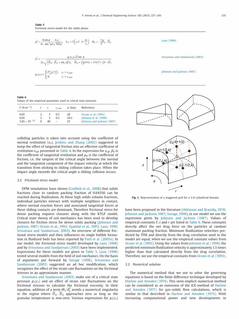
Table 5Frictional stress model for the solids phase.

μfs ¼6 sinϕ

9� sin 2ϕ

I11j j2

ffiffiffiffiffiffiffiffiffiffiffiffi3 IIDj j

p ; I11 ¼ 3 λs∇Uv�psεs

� �IID ¼�1

2D ij : D ij

Laux (1998)

μfs ¼pc εsð Þ

ffiffiffi2

psin ϕ

2εs

ffiffiffiffiffiffiffiffiffiffiffiffiffiffiffiffiffiffiffiffiffiffiffiffiffiffiffiffiffiffiffiffiffiffiffiffiffiffiffiffiffiffiffiffiffiffiffiffiffiffiffiffiffiffiffiffiffiffiffiffiffiffiffiffiffiffiffiffiffiffiffiffiffiffiffiffiffiffiffiffiffiffiffiffiffiffiffiffiffiffiffiffiffiffiffiffiffiffiffiffiffiffiffiffiffiffiffiffiffiffiffiffiffiffiffiffiD ij : D ij þ ðΘs=d

2s ÞÞ; D ij ¼ 1

2ðð∇vÞ þ ð∇vÞT Þ�13∇UvI Þ

r Srivastava and Sundaresan (2003)

pcðεsÞ ¼Fðεs�εs;min Þrðεmax

s �εs Þs ; εs4εs;min

0; εsoεs;min

8<:

Johnson and Jackson (1987)

Table 6Values of the empirical parameter used in critical state pressure.

F (N m�2) r s εs,min ϕ (deg) References

0.05 2 3 0.5 28 Ocone et al. (1993)0.05 2 5 0.5 28.5 Johnson et al. (1990)3.65�10�32 0 40 – 25 Johnson and Jackson (1987)

r

z

(i,j,k+1/2)

(i-1/2,j, k)(i,j -1/2,k)

(i,j+1/2,k)

Fig. 1. Representation of a staggered grid for a 3-D cylindrical domain.

V. Verma et al. / Chemical Engineering Science 102 (2013) 227–245 231

numerical methods, several modifications have been made toobtain robust and more accurate numerical models. In this work,special attention was paid to enhancing the stability and speed ofthe method. A two-step projection method has been used toobtain simultaneous solution for the momentum equations. Thetraditional solution method may get unstable at low values of thecoefficient of restitution, due to the tendency of inelastic particlesto concentrate in high-density clusters and strong non-linearity ofthe particle pressure near the maximum packing density. In suchcases unacceptable low time-steps of 10�6 s or less are required.To overcome this problem, a pressure and volume fraction (p–ε)correction algorithm is applied (Van der Hoef et al., 2006). In thisalgorithm, the compressibility of the solids phase is directly takeninto account in each computational cycle, while calculating thenew particle volume fraction. The SIMPLE algorithm of Patankarand Spalding (1972) is used to solve the pressure and volumefraction correction equations. Incorporation of the frictional modelfor dense phase regions further enhances the stability and com-putational speed of the code. Details of the solution method andboundary conditions will be explained later in this section. In thiswork, we only describe the model for the 3-D cylindrical coordi-nates system. However, the same methodology can also be appliedfor a Cartesian coordinate system, with only some differences inthe boundary conditions and the omission of terms related tocentrifugal-like and Coriolis-like forces. The inclusion of a cylind-rical wall in a Cartesian coordinate system would require the useof a cut cell method. However, evaluation of such a system isbeyond the scope of this work.

3.3.1. Representation of the flow domainThe domain of interest is represented by a number of fixed

Eulerian cells through which the gas–solid dispersion moves.Representation of a single cell is shown in Fig. 1. The cell interfacesin the r–θ plane and the r–z plane have toroidal and rectangularshapes respectively. The cells are labeled by indices i, j, and k,located at the cell center. A staggered grid arrangement is used,where the scalar variables (porosity, pressure, density, viscosityand granular temperature) are defined at the cell centers, whereasthe vector quantities (velocities) are defined at the cell face. Simplelinear interpolations have been used whenever variables arerequired at other locations. The computational grid in the cylind-rical domain forms a rectangular matrix in computational space.This rectangular matrix is enforced with a periodic boundarycondition (see Section 3.3.2.1) at the radial grid line where θ¼0and θ¼2π.

3.3.2. Initial and boundary conditionsAs an initial condition the solid velocities are set to zero and

the gas velocity is set with respect to the inflow boundaryconditions. Boundaries of the physical domain are representedby fictitious cells surround the computational domain. For acylindrical domain these fictitious cell lie at i¼0, i¼nr+1, k¼0

and k¼nz+1 where nr and nz are the total number of cells in radialand axial directions respectively. Scalar variables at these bound-aries are explicitly taken into account; data in these cells are up-dated during each iteration and computational cycle. Velocitycomponents are implicitly taken into account within the discre-tized flow equations. For example, the axial velocity component isemployed implicitly using

ðug;zÞi;j;k�12¼ aðug;zÞi;j;kþ1

2þ bðug;zÞi;j;kþ3

2þ c ð6Þ

In the above relationship, k¼0 defines a boundary condition (BC)at the bottom of the domain whereas the coefficients a, b, and cdepend on the type of BC. For instance, for inflow a and b are set tozero and c is set equal to the axial inflow velocity. Similarly, forfirst order no slip BC, a¼�1 and b¼c¼0 (for tangential compo-nents). Eq. (6) also allows us to use higher order BCs, where valuesof coefficients a, b and c are calculated depending upon the natureof the problem.

Table 7 shows different boundary conditions implemented inour code. These boundary conditions can be applied, by specifyingthe value of a cell flag fl(i,j,k) which is associated with relevantboundary conditions for cell i,j,k. Details of some of these bound-ary conditions have been reported by Kuipers et al. (1993).Additional boundary conditions required for the cylindrical systemare discussed in this section.

In order to break the numerical symmetry quickly after thestart of the simulation, a small random perturbation was added tothe initial solids fraction. A random small fluctuation in the inletvelocity can also be set in our model, to gain realistic inflow,similar to what is expected in experiments due to non-uniformities of the bottom plate.

3.3.2.1. Periodic boundary. Because we use a cylindrical grid, aperiodic BC is applied for flow crossing the boundary at θ¼0 orθ¼2π. All scalar and vector variables are incorporated implicitly atthis boundary, hence no fictitious boundary cells are required atθ¼0 or θ¼2π. This implicit incorporation of periodic BC willsubsequently contribute to the construction of an additional pairof diagonals in the resulting sparse matrix problem.

3.3.2.2. Axis boundary conditions. In reality there is no physicalboundary at the center of a fluidized bed reactor but numericallyan axis boundary condition (at r¼0) is applied to the velocitycomponents and the scalar quantities. At first sight, a free slipboundary condition for tangential components could be anapplicable solution, including a vanishing normal velocity at theaxis. However when these conditions are applied, we observedunrealistic behavior at the axis such as solids accumulation andthe distorted shapes of the bubbles. Bubbles prefer to stay awayfrom the axis (deflect towards the inner computational domain),rather than naturally crossing the axis. Some of these difficultieswith axis-symmetric cylindrical coordinates have been circum-vented by other researchers (Ma et al., 1998; Akselvoll and Moin,1996; Fukagata and Kasagi, 2002; Morinishi et al., 2004) mainlyfor single phase turbulent flow. Sun and Gidaspow (1999) alsoobserved the same effects for circulating fluidized bed riser flow,when using axis-symmetric 2-D cylindrical coordinates. Theyapplied a suitable remedy to their problem by employing adifferent grid structure near the central axis, integrating theequations from –r to +r. This approach seems to be unrealistictoo, as no information can travel through the axis. Moreover, adifferent combination of grid systems leads to different sets offlow equations that need to be connected at the interfaces of thegrids. These approaches are not only computationally expensivebut also very cumbersome for multiphase flow systems.

Table 7Boundary conditions.

Flag: 1 interior cellFlag: 2 free-slip for gas and particlesFlag: 3 no-slip for gas and particlesFlag: 4 prescribed influx for gas and particlesFlag: 5 prescribed pressure for gas and permeable free-slip for particlesFlag: 6 zero-gradient outflow for gas and particlesFlag: 7 no-slip for gas and partial-slip for particlesFlag: 8 no-slip for gas and free-slip for particlesFlag: 9 corner cellFlag: 10 prescribed pressure for gas and permeable no-slip for particlesFlag: 11 Periodic flow for gas and particles.

V. Verma et al. / Chemical Engineering Science 102 (2013) 227–245232

Our staggered grid arrangement proves to be advantageous fortreatment of the axis because no scalar variable or velocity compo-nent lies at the axis, except the radial velocity component (ur). Fig. 1shows that a staggered variable near the axis (i.e. at Δr/2) can beconnected to the boundary by using information from the cell at theopposite side of the axis. Only the radial velocity component at theaxis needs a special treatment, for apparent radial flow communica-tion through the axis without influence to or from points atneighboring θ locations. In this work we tried different approachesto minimize numerical artifacts at the axis. A cross-analysis (fromporosity visualization) for different axis treatments at different flowconditions reveals that numerical artifacts at the axis are negligiblewhen radial momentum is taken into account across the axis. Thistreatment is very similar to Morinishi et al. (2004), who introducedan averaged value of the radial velocity component at the axis.Similarly we define the radial momentum of each phase at the axis

as equal to the mean momentumwith its neighboring cell across theaxis, represented by Eqs. (7) and (8).

½ερðΔr=2;θ; zÞ þ ερðΔr=2;θ þ π; zÞ�2

urð0;θ; zÞ ¼½ερurðΔr;θ; zÞ�ερurðΔr;θ þ π; zÞ�

2ð7Þ

The negative sign in the RHS of Eq. (7) accounts for the reversal ofthe radial direction at θ+π. Therefore the radial velocity componentat the axis is defined as

urð0;θ; zÞ ¼½ερurðΔr;θ; zÞ�ερurðΔr;θ þ π; zÞ�½ερðΔr=2;θ; zÞ þ ερðΔr=2;θ þ π; zÞ� ð8Þ

This approach may lead to a multi-value of ur at the axis, as differentvalues of ur are obtained for different values of θ (taking into accountthe different orientations of the cells). We also tried a single valueapproach proposed by Fukagata and Kasagi (2002), in combinationwith the above approach but results (visualization of porosity plot)reveal no improvement compared to the above approach. So in thiswork we opt for the above (Eq. (8)) approach, but a single valueapproach has also been implemented in our model.

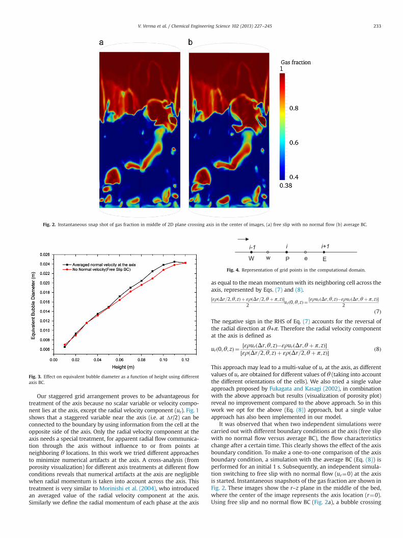
It was observed that when two independent simulations werecarried out with different boundary conditions at the axis (free slipwith no normal flow versus average BC), the flow characteristicschange after a certain time. This clearly shows the effect of the axisboundary condition. To make a one-to-one comparison of the axisboundary condition, a simulation with the average BC (Eq. (8)) isperformed for an initial 1 s. Subsequently, an independent simula-tion switching to free slip with no normal flow (ur¼0) at the axisis started. Instantaneous snapshots of the gas fraction are shown inFig. 2. These images show the r–z plane in the middle of the bed,where the center of the image represents the axis location (r¼0).Using free slip and no normal flow BC (Fig. 2a), a bubble crossing

Fig. 2. Instantaneous snap shot of gas fraction in middle of 2D plane crossing axis in the center of images, (a) free slip with no normal flow (b) average BC.

Fig. 3. Effect on equivalent bubble diameter as a function of height using differentaxis BC.

W EP ew

i i+1i-1

Fig. 4. Representation of grid points in the computational domain.

V. Verma et al. / Chemical Engineering Science 102 (2013) 227–245 233

the axis is not properly connected, but rather shows splitting. Thismay be due to accumulation of the solid phase near to the axis.However when the average normal velocity at the axis is applied(Fig. 2b), the bubble shows continuous attachment at the axis.

An analysis of the effect of the axis BC has been made as wellon a time-average scale, by measuring the equivalent bubblediameter with height. Fig. 3 shows a difference in bubble size,applying different axis BC as discussed above. With no normalvelocity at the axis, a lower bubble size is predicted above a heightof 5 cm. This may be due to splitting of the bubble, creatingsmaller bubbles. No significant difference in bubble size in thebottom region of the bed is observed. This may be because smallbubbles are mostly formed near to the wall of the bed.

3.3.2.3. Partial slip. Tangential velocities and pseudo-granulartemperature for partial slip BC at the wall can be obtained bycalculating values of coefficients a, b and c in Eq. (6). Relations forthe solids velocity gradient at the wall have been given by Sinclairand Jackson (1989). Details of this BC and implementation havebeen given by Nieuwland (1995).

3.3.3. Discretization of convection termsMass, momentum and granular flux have been discretized

using total variation diminishing (TVD) methods such as MINMOD.Other variables such as pressure, viscosity and time derivativeshave been discretized using a central differencing scheme. Theconcept of a flux limiter function is used to construct highresolution schemes (TVD). The idea is to mix the numerical fluxof higher order and lower order schemes using a flux limiterfunction in such a way that the resulting scheme gives higherorder accuracy in smooth regions of the flow and sticks with firstorder accuracy in the vicinity of physical discontinuities.

Description of the TVD schemes using flux limiter functions isexplained for the case shown in Fig. 4. Flux limiters for differentTVD are presented in Table 8. Standard notation is used for thisexplanation; however notation used on staggered grids is alsoshown in Fig. 4. The value at the position “e” is affected by itsneighboring points, so the effective value at “e” can be interpo-lated using higher order interpolation, considering that thevalue should lie within a TVD region of the Sweby flux-limiterdiagram (Sweby, 1984; Waterson and Deconinck, 2007). Thereforea representation of the value at position “e” is given by

ϕe ¼ϕP þ ð1=2Þψ ðreÞðϕE�ϕPÞ ð9Þwhere ψ(ri) is the flux limiter function as a function of re, where reis given by

re ¼ϕP�ϕW

ϕE�ϕPð10Þ

A singularity may be expected in solving the discretized forms ofthe governing equations at the central axis, when r equals zero.However discretizing the governing equations on a cylindricalforward staggered arrangement, reveals that no singularity is

encountered, except for the stress component τθr in the radialmomentum equation, which is assumed to be zero at the axis.

3.3.4. Solution methodA semi-implicit methodology is used to solve the governing

equations. For convenience, the time discretization is shown here.The time discretization of the continuity and momentum equa-tions is given by

ðεmρmÞnþ1 ¼ ðεmρmÞn�Δt ∇U ðεmρmumÞ� �nþ1 ð11Þ

ðεmρmumÞnþ1 ¼ ðεmρmumÞn�Δtðεm∇pgÞnþ1�Δtð∇pmÞnþ1

þAn þΔtβnðug�usÞnþ1 þΔtðεmρmgÞn ð12Þhere subscript m represents the phase (either gas or solids) andsuperscript n denotes the time index. Note that in Eq. (12), thethird term on the RHS is only included for the solids phase (for thegas phase this term drops out) and that the inter-phase momen-tum exchange term changes its sign for the gas phase. An in theequation collectively represents convection and viscous interac-tion terms. The superscript * denotes that these terms are takeninto account semi-implicitly, where for each direction the normalderivative of convection and viscous interaction are treatedimplicitly whereas mixed derivatives are taken explicitly. Adeferred correction (DC) has been incorporated in the convectionterms to offer stability to the solution. In the solution of thealgebraic equations, DC uses a lower order (upwind (UW)) methodimplicitly and a higher order (TVD) method explicitly. The DCformulation for the convection term is given by Eq. (13). Such aformation still leads to a diagonally dominant sparse matrix, andprovides a stable solution with better convergence.

An

conv: ¼ Anþ1conv:;UW þ ðAn

conv:;TVD�Anconv:;UW Þ ð13Þ

The solution to the momentum equation (Eq. (12)) for both phasesis obtained through a two-step projection method. For this Eq. (12)is re-written as

ðεmρmumÞnþ1 ¼ ðεmρmumÞnn�Δtðεm∇pgÞnþ1�Δtð∇pmÞnþ1

þΔtβnðug�usÞnþ1 ð14Þwhere

ðεmρmumÞnn ¼ ðεmρmumÞn þ An þΔtðεmρmgÞn ð15ÞIn a first step, tentative momentum fields are calculated fromEq. (15). Subsequently, the velocity fields are calculated using thecoupled momentum equations (Eq. (14) for both phases). Next, thep–ε method is used for calculating the corrected pressure andsolids volume fraction.

The pressure correction equation is given by

ðJgÞni�1;j;kðΔPgÞi�1;j;k þ ðJgÞniþ1;j;kðΔPgÞiþ1;j;k þ ðJgÞni;j�1;kðΔPgÞi;j�1;k

þðJgÞni;jþ1;kðΔPgÞi;jþ1;k þ ðJgÞni;j;k�1ðΔPgÞi;j;k�1 þ ðJgÞni;j;kþ1ðΔPgÞi;j;kþ1

þðJgÞni;j;kðΔPgÞi;j;k ¼�ðDgÞni;j;k ð16Þ

where Jng represents the Jacobi matrix for the gas phase. This matrixcontains the derivatives of the mass residual Dg with respect to the gasphase pressure, for which explicit expressions can be obtained fromthe continuity equation (Eq. (11)) for the gas phase in combinationwith the momentum equations (Eq. (12)). To save computationaleffort, the elements of the Jacobi matrix are evaluated at the old timelevel. The solution procedure for Eq. (16) is exactly the same as theSIMPLE procedure of Patankar and Spalding (1972).

Having obtained the corrected pressure, the new velocities arecalculated from the coupled momentum equations, and new solidsvolume fractions are obtained from the solids phase mass balance.Only then the new solids pressures are determined, whichregularly leads to excessive compaction and extremely high

Table 8Flux limiter functions.

TVD Limiter function ψ(r) Source

Minmod minðr;1Þ if r400 if rr0

(Roe (1986)

Superbee max½0; minð2r;1Þ; minð2; rÞ� Roe (1986)

Upwind 0Central differencing 1

V. Verma et al. / Chemical Engineering Science 102 (2013) 227–245234

particle pressures in areas where the particle packing densities areclose to random close packing. Therefore we employ a volumefraction correction procedure, which computes the particlevolume fractions, taking the compressibility of the solids phasemore directly into account. Similar to the pressure correction forthe gas phase, a whole field particle volume fraction correction iscomputed, satisfying

ðJsÞni�1;j;kðΔεsÞi�1;j;k þ ðJsÞniþ1;j;kðΔεsÞiþ1;j;k þ ðJsÞni;j�1;kðΔεsÞi;j�1;k

þðJsÞni;jþ1;kðΔεsÞi;jþ1;k þ ðJsÞni;j;k�1ðΔεsÞi;j;k�1 þ ðJsÞni;j;kþ1ðΔεsÞi;j;kþ1

þðJsÞni;j;kðΔεsÞi;j;k ¼�ðDsÞni;j;k ð17Þ

where now Jns represents the derivative of the solid phase masswith respect to the solid volume fraction. Eqs. (16) and (17) aresolved for the whole computational domain, and form two sparsematrix equations. The solution to such matrix equations isachieved using a conjugate gradient method. After the new solidsvolume fractions have been obtained from Eq. (17), new solidspressures are calculated after which new velocities are calculatedfrom the coupled momentum equations. Subsequently, the gran-ular temperature equation (Eq. (T1-5)) is solved by an iterativeprocedure. In Eq. (T1-5), terms representing convective transportand generation of fluctuation kinetic energy by viscous shear aretreated explicitly. The granular energy dissipation term is treatedsemi-implicitly, whereas all other terms are treated fully implicitly.

4. Results and discussions

A TFM simulation generates output in matrix form, with outputvariables on a regular computational grid. These output variablesinclude solids volume fraction, velocity components of each phase,the gas phase pressure, and the granular temperature. Other

Table 9TFM simulation setting for comparison with experimental work.

Particle type: GlassParticle density 2500 kg m�3

Particle diameter 0.5 mmCoefficient of restitution 0.86Minimum fluidizing velocity (Umf) 0.18 m s�1

Superficial velocity 3.5Umf

Gas–particle drag Van der Hoef et al. (2005)The frictional model Srivastava and Sundaresan (2003)Flux limiter Superbee (Roe, 1986)Flow solver time-step 10�4 s

Table 10Bed size specification for comparison withexperimental work

Bed diameter (m) 0.306Overall height of the domain (m) 0.816Initial particle bed height (m) 0.45Numbers of grids in the r-direction 45Numbers of grids in the θ-direction 30Numbers of grids in the z-direction 240

Table 11Bed size specification in the simulations.

Bed diameter (m) 0.10Overall height of the domain (m) 0.30Initial particle bed height (m) 0.125Numbers of grids in the r-direction 20Numbers of grids in the θ-direction 20Numbers of grids in the z-direction 120

Fig. 5. Instantaneous snapshot of volume fraction of gas in the middle of 3-D bed at (a) t¼2.6, (b) t¼4.0 and (c) t¼5.0 s (simulation setting in Tables 9 and 10).

V. Verma et al. / Chemical Engineering Science 102 (2013) 227–245 235

quantities of interest can be calculated from these variables, suchas the average particle bed height, average pressure drop andbubble characteristics.

Different test simulations were carried out to show the validity ofthe model. We compare the TFM simulations with experimentalwork from the literature for a full 3-D cylindrical domain. Specifically,Laverman et al. (2012) have used PEPT experimental techniques tostudy the behavior of different types of particles (glass and LLDP) atdifferent superficial velocities, for two different initial particle bed

Fig. 6. 3-D contours plot for the gas phase (εg¼0.7) for same instantaneous snapshot as shown in Fig. 5.

Fig. 7. TFM and experimental comparison of the azimuthally and time-averagedlateral profile of solids axial velocity at three different heights above the distributor.

Fig. 8. Azimuthally and time-averaged solids circulation patterns, (a) experiments(Laverman et al., 2012) (b) TFM simulations.

V. Verma et al. / Chemical Engineering Science 102 (2013) 227–245236

heights in a 30.6 cm diameter column. We compare one of theirmeasurements with our simulations in Section 4.1. Our simulationssettings correspond to their experimental setup and operatingconditions, as presented in Tables 9 and 10.

In this work we have introduced different TVD schemes.Comparisons between two TVD schemes (Section 4.3) were carriedout for a specific case of initial particle bed height of 30 cm and asuperficial gas velocity of 2.5Umf. Investigation of the effects of thefrictional model (Section 4.4), grid refinement (Section 4.2), andcoefficient of restitution (Section 4.5) were carried out indepen-dently for a particle bed height of 12.5 cm. Other simula-tion settings for the bed dimensions are presented in Table 11.The numerical setting and particle properties are the same as inTable 9, except for the superficial gas velocity which was set to 2.5Umf.

The comparisons are based on the equivalent bubble diameter asa function of height from the distributor plate. Here the equivalentbubble diameter is calculated as a number and time-average,assuming the area of a bubble detected in cross-sections (r–θ plane)at different heights to be circular. A gas fraction of 0.80 is assumedto define the bubble boundary and a linear interpolation techniqueis used to calculate the precise position of the boundary in the sharpgradient between bubble and emulsion phase. Along with thebubble size, the bubble number distributions at different heights

are compared. Instantaneous snapshots are shown in a verticalplane through the middle of the 3-D bed. Particle characteristics arecompared for solids circulation patterns and solids axial velocity onan azimuthally and time-averaged scale. Eq. (18) shows the expres-sion for azimuthally and time-averaging axial velocity, where ⟨ ⟩ and∑ shows azimuthally-averaging and time-averaging respectively.Time-averaging is performed for a total time of 10 s, ignoring theinitial fist second to avoid inclusion of start-up effects.

uavgz;s ¼∑ΔtA t εsuz;s

� �Δt

∑ΔtA t εsh iΔtð18Þ

4.1. Comparison between TFM simulation and experimental results

We first compare our simulations with the experimental work ofLaverman et al. (2012). Fig. 5 shows instantaneous snapshots of thegas fraction in a vertical plane in the middle of the bed. Fig. 6 shows3-D gas fraction contours in the 3-D domain. These figures clearlyshow that small bubbles originate at the bottom of the bed, grow insize due to coalescence and move towards the central axis due to alower resistance at the center (Kunii and Levenspiel, 1991).

Fig. 7 shows the azimuthally and time-averaged axial velocityprofile of the solids phase at three different heights in the fluidizedbeds. At the bottom section of the bed, particles show descendingbehavior near the central axis and ascending behavior near thewalls. The prediction in the top section of the bed is just theopposite. This is due to the formation of two vortices above oneanother in the particle bed. Fig. 8 shows the azimuthally and time-averaged solids circulations pattern predicted from TFM simulation.For clarity, not all vectors are shown, but only every alternate vectorin the radial direction and axial direction. The particle motion isgoverned mainly by the motions of the bubbles, because the

Table 12Grid refinement test.

Direction Number of grid cells Grid size (mm, rad, mm)

Base case 20�20�120 2.5�2π/20�2.5Radially refined 32�20�120 1.5625�2π/20�2.5Azimuthally refined 20�32�120 2.5�2π/32�2.5

Fig. 9. Instantaneous snapshot of gas fraction in the middle of 3-D bed at t¼0.5 s, for grids (a) 20�20�120, (b) 20�32�120 and (c) 32�20�120, in radial, azimuthallyand axial directions respectively.

V. Verma et al. / Chemical Engineering Science 102 (2013) 227–245 237

moving bubbles carry particles with them in their wakes. Densephase surrounding wakes of the bubble tries to shed those particlesfrom the bubble wakes. Our results indicate that bubbles generallyoriginate at the bottom, near the wall boundary, grow in size andtend to move towards the center of the bed due to a lowerresistance. Eruption of the bubble in the freeboard regions generallytakes place in the center of the bed, and particles generally descendnear to the wall, leading to an overall circulation of particles. Overallthis motion of bubbles and particles follows an “S”-like structure.

Figs. 7 and 8 show that the TFM simulation results are veryclose to the experimental observations. The centers of bothvortices (Fig. 8) are approximately at the same locations as inthe experiments. The TFM simulations results are in very goodagreement at a height of 31 cm from the bottom of the distributor.Small deviations in the TFM results are observed at heights of21 cm and 11 cm (see Fig. 7). This can be explained from Fig. 8. Theheight of 21 cm lies at the separation region between two vortices,and is therefore somewhat more prone to deviations.

The axial velocity profiles near the walls show larger deviations atall heights. This may be due to the partial-slip boundary conditionsused for the particle phase at the wall. The simulationwas performedon a relatively coarse grid (3.5 mm). With refinement of the grid size,the results are expected to come to closer agreement with experi-mental results. The effect of grid refinement (using a finer grid on asmaller system) is presented in the next section.

4.2. Grid independence

We now turn to a smaller system, for which the base case isdescribed in Table 11. A grid (in)dependency test is carried outwith refinement of the grid in radial and azimuthal directionsindependently. The different combination of grids is given inTable 12.

Fig. 9 shows instantaneous snapshots of the gas fraction for thedifferent grid combinations. When grids are refined in the azimuthaldirection, no significant differences are observed. However refinementin the radial direction shows considerable differences in the instanta-neous images. A comparison of the time-averaged bubble size,averaged over a total time of 10 s, is presented in Fig. 10. Fig. 10(a) shows that the change in the equivalent bubble diameter atdifferent grid size combinations does not show major differences.The predicted number of bubbles as a function of height is shown inFig. 10(b). The number of bubbles is significantly larger when a gridrefinement is performed in azimuthal and radial directions. When thegrid is only refined in the radial direction many smaller bubbles arepredicted in the bottom section of the bed. These grid refinement tests

show that refinement in the radial direction is much more importantthan refinement in the azimuthal direction. A grid independentsolution could be established with the number of radial grids equalto 32 and the number of azimuthal grids between 20 and 32. We alsonote that that excessive refinement in the azimuthal direction leadsto very small grids near the central axis, resulting in convergenceproblems.

4.3. Effects of the flux-limiter function

To increase the accuracy of the numerical solution, one can notonly refine the grids but also make use of higher order discretizationschemes for the convection terms. The superiority of higher orderdiscretization schemes is no point of doubt when compared withfirst-order differencing schemes or upwind schemes (FOU). Althoughfirst-order schemes are highly diffusive, they still find use in CFD dueto their stability and fast convergence. However, the higher orderschemes provide more accurate solutions with less numerical diffu-sion. Various higher order schemes exist, and all lie within a TVDregion of the Sweby flux-limiter diagram (Sweby, 1984; Watersonand Deconinck, 2007). A flux limiter function is used to implementthese schemes (see Section 3.3.3). In this work we will compare theMinmod and Superbee schemes, because they cover the lower boundand upper bound of the TVD region, respectively. Both these schemes

Fig. 10. Comparison on grid refinement, (a) equivalent bubble diameter as a function of height and (b) bubble distribution as a function of height.

Fig. 11. Azimuthally and time-averaged lateral profiles of the axial solids velocity atthree different heights from the bottom. Results of Laverman et al. (2012),compared with simulations using Superbee and Minmod limiters.

V. Verma et al. / Chemical Engineering Science 102 (2013) 227–245238

are composites of the upper differencing scheme (UDS), centraldifferencing scheme (CDS) and linear upwind scheme (LUS). TheSuperbee scheme was designed to achieve the best possible resolu-tion of discontinuities, whereas the Minmod scheme seems to benumerically diffusive (Waterson and Deconinck, 2007). Consideringthis, we have tested both schemes for gas–solids flow, where a highresolution is required in the vicinity of the different phases.

Fig. 11 shows azimuthally and time-averaged axial solidsvelocity profiles computed at three different heights in compar-ison with the experimental results of Laverman et al. (2012) usingthe two different flux limiters. The results obtained from theSuperbee limiter are in close agreement with the experimentalresults. A major difference in the solids axial velocity profile isobserved at a height of 0.31 m from the bottom. At this height, theMinmod limiter predicts approximately zero solids velocity near

the center. This is also evident from the solids circulation patternin Fig. 12, where the Minmod limited predicts no solids motionabove a height of 30 cm near the center. However, Laverman et al.(2012) observed a higher solids axial velocity at this height. Thisobservation is in close resemblance with our results using theSuperbee flux-limiter. Since the solids motion is directly governedby bubble flow, further explanation of this behavior should besought in the differences with respect to the bubble characteristicspredicted by both schemes.

Fig. 13(a) shows the equivalent bubble diameter as a function ofheight, comparing the two limiters. The Superbee limiter predictsa larger bubble size above a height of 0.15 m. Fig. 13(b) reveals thatconsiderably more bubbles are predicted by the Superbee limitercompared to the Minmod limiter at the bottom section of thefluidized bed. Fig. 14 shows the bubble size distribution at a height

Fig. 12. Azimuthally and time-average solids axial velocity vectors. (a) Experimental results (Laverman et al., 2012), (b) Superbee flux limiter and (c) Minmod flux limiter.

Fig. 13. Comparisons on Superbee and Minmod flux-limiter, (a) Bubble size as a function of height and (b) Bubble number distribution as a function of height.

V. Verma et al. / Chemical Engineering Science 102 (2013) 227–245 239

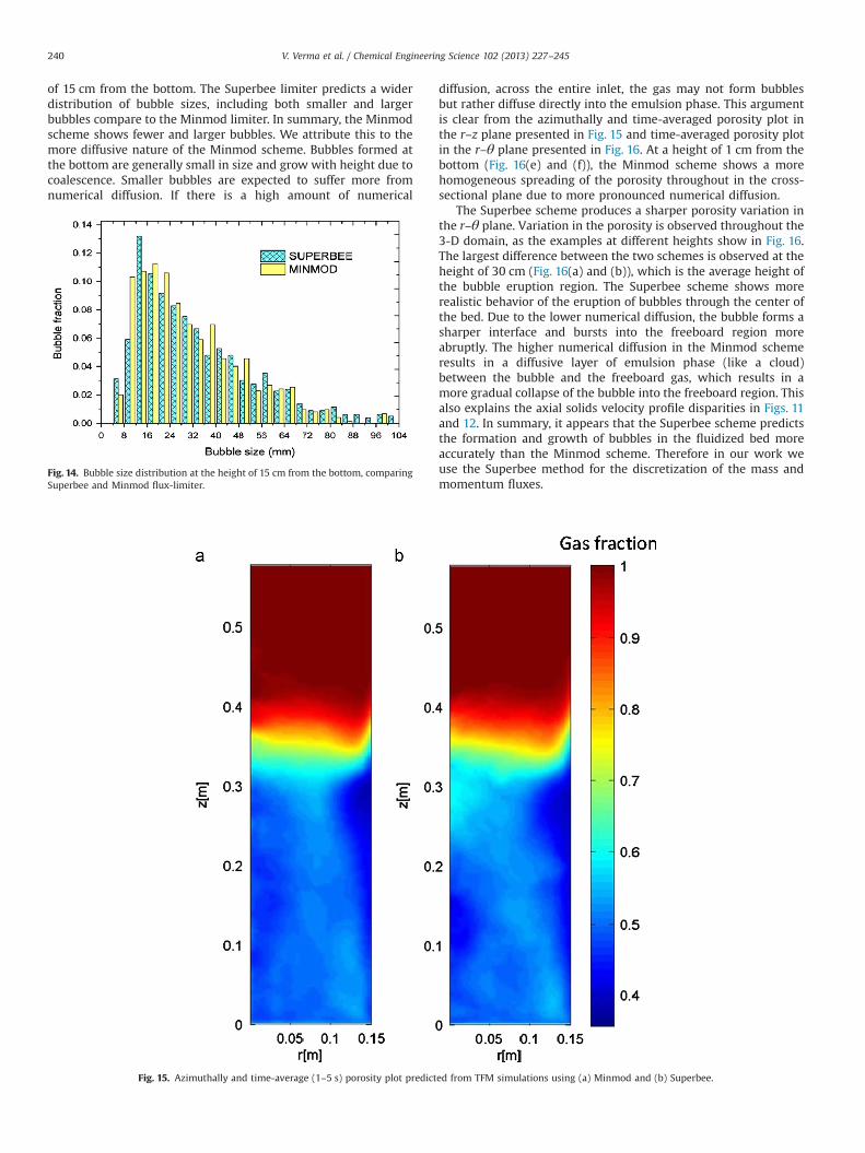
of 15 cm from the bottom. The Superbee limiter predicts a widerdistribution of bubble sizes, including both smaller and largerbubbles compare to the Minmod limiter. In summary, the Minmodscheme shows fewer and larger bubbles. We attribute this to themore diffusive nature of the Minmod scheme. Bubbles formed atthe bottom are generally small in size and grow with height due tocoalescence. Smaller bubbles are expected to suffer more fromnumerical diffusion. If there is a high amount of numerical

diffusion, across the entire inlet, the gas may not form bubblesbut rather diffuse directly into the emulsion phase. This argumentis clear from the azimuthally and time-averaged porosity plot inthe r–z plane presented in Fig. 15 and time-averaged porosity plotin the r–θ plane presented in Fig. 16. At a height of 1 cm from thebottom (Fig. 16(e) and (f)), the Minmod scheme shows a morehomogeneous spreading of the porosity throughout in the cross-sectional plane due to more pronounced numerical diffusion.

The Superbee scheme produces a sharper porosity variation inthe r–θ plane. Variation in the porosity is observed throughout the3-D domain, as the examples at different heights show in Fig. 16.The largest difference between the two schemes is observed at theheight of 30 cm (Fig. 16(a) and (b)), which is the average height ofthe bubble eruption region. The Superbee scheme shows morerealistic behavior of the eruption of bubbles through the center ofthe bed. Due to the lower numerical diffusion, the bubble forms asharper interface and bursts into the freeboard region moreabruptly. The higher numerical diffusion in the Minmod schemeresults in a diffusive layer of emulsion phase (like a cloud)between the bubble and the freeboard gas, which results in amore gradual collapse of the bubble into the freeboard region. Thisalso explains the axial solids velocity profile disparities in Figs. 11and 12. In summary, it appears that the Superbee scheme predictsthe formation and growth of bubbles in the fluidized bed moreaccurately than the Minmod scheme. Therefore in our work weuse the Superbee method for the discretization of the mass andmomentum fluxes.

Fig. 15. Azimuthally and time-average (1–5 s) porosity plot predicted from TFM simulations using (a) Minmod and (b) Superbee.

Fig. 14. Bubble size distribution at the height of 15 cm from the bottom, comparingSuperbee and Minmod flux-limiter.

V. Verma et al. / Chemical Engineering Science 102 (2013) 227–245240

4.4. Effect of the frictional model

We now turn to the requirement of an additional frictionalclosure for dense phase regions in the TFM. We will compare thefrictional stress models of Srivastava and Sundaresan (2003) andLaux (1998). The main difference between these two models isthat additional frictional normal stresses were ignored by Laux(1998). The model of Laux (1998) calculates the frictional viscosityfrom kinetic and collisional contributions in the KTGF, instead ofusing a semi-empirical expression for the critical state pressurewith respect to the solids volume fraction. This may lead toconvergence problems due to divergence of the radial distributionfunction (see Eqs. (3) and (4)) close to maximum packing. A fixedvalue for the solids viscosity is used otherwise. From our simula-tions we observed that the number of iterations to reach conver-gence reduced significantly using the Srivastava and Sundaresan(2003) model, whereas the Laux (1998) model was found to benumerically unstable and fails to reach convergence at someoperating conditions.

Fig. 17(a) and (b) shows instantaneous snapshots of the gasvolume fraction obtained using Laux (1998) and Srivastava andSundaresan (2003), respectively. The Laux (1998) model predictsvery much diffusive bubbles, i.e. excessive gas from the bubblediffuse into the emulsion phase through the bubble interface. Thisbehavior may be due to additional frictional stresses because ofsolids fluctuations ignored by Laux (1998). This directly affects theporosity distribution near to the bubble surface, leading toexcessive leakage of gas through the bubble boundary. TheSrivastava and Sundaresan (2003) model predicts a sharp bubble

Fig. 16. Time-averaged (1–5 s) porosity plot in r–θ plane at three different heightsfrom the bottom, comparing Minmod and Superbee flux limiter. (a) h¼30 cm forMinmod, (b) h¼30 cm for Superbee, (c) h¼14 cm for Minmod, (d) h¼14 cm forSuperbee, (e) h¼1 cm for Minmod and (f) h¼1 cm for Superbee.

Fig. 17. Instantaneous snapshot of gas fraction at t¼0.5 s (a) Laux (1998) and (b)Srivastava and Sundaresan (2003).

Fig. 18. Azimuthally and time-averaged solids flow patterns predicted using thefrictional model from (a) Srivastava and Sundaresan (2003) and (b) Laux (1998).

V. Verma et al. / Chemical Engineering Science 102 (2013) 227–245 241

interface and dense regions are much more pronounced. Fig. 19(a) shows the effect on the predicted equivalent bubble diameterusing the two frictional models. Almost the same average bubblesize is predicted with both models in the bottom section of thebeds. At larger height, there is a significant difference in averagebubble size. The Srivastava and Sundaresan (2003) model predictsa larger bubble size compared to the Laux (1998) model. Fig. 19(b) shows that the number of bubbles predicted by the Laux (1998)model is higher throughout the bed. This may be due to smallpores forming in the dense phase (see Fig. 17(a)) which are

counted as bubbles, with a considerable effect on the measuredbubble size as well as the bubble distribution.

Fig. 18(a) and (b) shows the azimuthally and time-averagedsolids circulation pattern predicted using the two frictional mod-els. The main difference can be seen in the formation of the uppervortex. The particle velocity and average particle circulation heightis higher in the case of the Srivastava and Sundaresan (2003)model. Very different particle flow patterns are predicted in theregion between the lower and upper vortex. This shows thedifference in the bubble dynamics in this region. The nature of

Fig. 19. Comparisons between Laux (1998) and Srivastava and Sundaresan (2003) frictional models. (a) Bubble size as a function of height and (b) bubble numberdistribution as a function of height.

Fig. 20. Effect of coefficient of restitution on bubble characteristics, (a) equivalent bubble diameter as a function of height and (b) bubble number distribution as a function of height.

Fig. 21. Root Mean Square (RMS) of (a) pressure drop fluctuations and (b) granular temperature, over the bed as a function of coefficient of restitution. Total time of 2–6 s.

V. Verma et al. / Chemical Engineering Science 102 (2013) 227–245242

the circulation pattern and the vortex formation are very close tothe experimental findings of Laverman et al. (2012) if theSrivastava and Sundaresan (2003) frictional stress model is used.In summary, the Srivastava and Sundaresan (2003) frictional stressmodel not only provides better numerical stability and fastconvergence but also predicts more realistic bubbles and particledynamics. Therefore in our work we use the Srivastava andSundaresan (2003) frictional stress model to take into accountdense solids phase regions in the fluidized bed.

4.5. Effect of the coefficient of restitution

To study the influence of the coefficient of restitution en on thehydrodynamics, simulations for various values of en representingnearly elastics to rough spheres (en¼0.97, 0.94, 0.90, 0.86, 0.77 and0.74) have been performed, keeping all other parameters fixed.Fig. 20(a) shows the change in bubble size with height from thebottom for different values of en. The average equivalent bubblediameter calculated for different values of the coefficient ofrestitution does not show a significant difference. However, thenumber of bubbles increases with decreasing coefficient of resti-tution (see Fig. 20(b)). This is due to the well-known fact thatstronger dissipations of fluctuating energy leads to creation ofmore and more bubbles. As the particle collisions become lessideal, inhomogeneities become more pronounced, resulting insharper porosity contours and larger bubbles.

Fig. 21(a) shows the root-mean-square pressure fluctuations asa function of the coefficient of restitution. We observe that thepressure fluctuations decrease gradually as the collisions becomemore elastic. Simultaneously, the granular temperature increases,as shown in Fig. 21(b). The same observations have been reportedby Goldschmidt (2001). KTGF (the original version) only takes intoaccount normal particle–particle collisions, ignoring the effects ofsliding friction. An effective coefficient of restitution may becalculated, taking the effects of sliding friction during collisioninto account (see Table 2). Goldschmidt (2001) finds that using theeffective value of the coefficient of restitution leads to closeresemblance of experimental results. For example, the coefficientof restitution for glass particles is 0.97, yet the effective restitutionof coefficient is 0.86. A significant difference in the bubble size,pressure and granular temperature is predicted for these twovalues of the coefficient of restitution. Therefore additional clo-sures, which incorporate tangential and rotational friction in theKTGF more accurately, are considered necessary.

5. Conclusion

A two-fluid model using KTGF closure has been numericallyintegrated on a three dimensional cylindrical coordinate system tostudy dense gas–solid flow. A highly efficient numerical scheme hasbeen incorporated to obtain a solution to the governing equations.This work has been initiated to enable computational studies oflarge scale gas–solid fluidized beds, further addressing industrialproblems. We have paid attention to increase the speed and stabilityof the code. A two-step projection method has been used to solvethe set of momentum equations, allowing us to take larger timesteps. A higher order discretization scheme, using flux limiters, isused for the momentum, mass and granular fluxes. Deferredcorrection provides stability and computational speed to the solu-tion, solving a linear form of the p–ε equations. The validity of theTFM approach is supported by comparison with experimentalresults from the literature. The axial velocity of the solids phasepredicted by TFM simulations is in close agreement with experi-mental observations of Laverman et al. (2012). For the first time, adetailed comparative study on numerical parameters is made for a

3-D cylindrical fluidized bed in the bubbling regime. Grid depen-dency tests show that refinement of the grid is more sensitive in theradial direction than the azimuthal direction. Results obtained usingthe frictional stress models of Laux versus Srivastava and Sundar-esan show that only the latter can properly predict the dynamics inthe dense phase regions. Comparison between Minmod andSuperbee flux limiters shows that the Minmod limiter is numericallydiffusive in nature, fails to predict smaller bubbles. A study of theeffect of the coefficient of restitution shows that KTGF is mostsuitable for nearly elastics collision. The bubble size increases withheight and increases in coefficient of restitution. Of course, the TFMfor fluidized bed is highly dependent upon the validity of the KTGFclosures. Hence further investigation is required for the KTGFclosures to include particle tangential and rotational friction. Never-theless, TFM is able to provide detailed insight in the behavior ofbubbles and the solids phase in 3-D fluidized beds.

Nomenclature

C fluctuation particle velocity, m s�1

g gravitational acceleration, m s�2

I unit tensor, dimensionlessp pressure, Paq kinetic fluctuation energy, kg s�1

u velocity, m s�1

t time, sen coefficient of restitutions, dimensionlessUmf minimum fluidizations velocity, m s�1

Greek symbols

β interphase momentum transfer coefficient, kg m�3 s�1

γ dissipation due to inelastic particles collisions,kg m�1 s�3

ε volume fraction, dimensionlessρ density, kg m�3

Θ pseudo-particles temperature, m2 s�2

τ stress tensor, Paμ shear viscosity, kg m�1 s�1

μ dynamic friction coefficient, dimensionless (used inTable 4 only)

Subscripts

s solid phaseg gas phasep particlem solid phase/gas phasemf minimum fluidizationmax maximumeff effective

Operator

∇ gradient∇∙ divergence

Acknowledgment

The authors would like to thank the European Research Councilfor its financial support, under its Advanced Investigator Grantscheme, Contract no. 247298 (MultiscaleFlows).

V. Verma et al. / Chemical Engineering Science 102 (2013) 227–245 243

References

Akselvoll, K., Moin, P., 1996. Large-eddy simulation of turbulent confined coannularjets. Journal of Fluid Mechanics 315, 387–411.

Anderson, T.B., Jackson, R., 1967. A fluid mechanical description of fluidized bed. I &EC Fundamentals 6 (4), 527–539.

Asegehegn, T.W., Schreiber, M., Krautz, H.J., 2012. Influence of two- and three-dimensional simulations on bubble behavior in gas–solid fluidized beds withand without immersed horizontal tubes. Powder Technology 219, 9–19.

Atkinson, H., Bransby, L., 1978. The Mechanics of Solids: An Introduction to CriticalState Soil Mechanics. McGraw-Hill, UK.

Beetstra, R., van der Hoef, M., Kuipers, J.A.M., 2007a. Drag force of intermediateReynolds number flow past mono- and bidisperse arrays of spheres. AIChEJournal 53, 489–501.

Brouwer, G.C., Wagner, E.C., Van Ommen, J.R., Mudde, R.F., 2012. Effects of pressureand fines content on bubble diameter in a fluidized bed studied using fast X-raytomography. Chemical Engineering Journal 207–208, 711–717.

Busciglio, A., Vella, G., Micale, G., Rizzuti, L., 2008. Analysis of the bubblingbehaviour of 2D gas solid fluidized beds. Part I. Digital image analysistechnique. Chemical Engineering Journal 140, 398–413.

Cammarata, L., Lettieri, P., Micale, G., Colman, D., 2003. 2D and 3D CFD simulationsof bubbling fluidized beds using Eulerian–Eulerian models. InternationalJournal of Chemical Reactor Engineering 1 (A48), 1–19.

Chapman, S., Cowling, T.G., 1970. The Mathematical Theory of Non-Uniform Gases,3rd ed. Cambridge University Press, Cambridge.

Cranfield, R.R., Geldart, D., 1974. Large particle fluidization. Chemical EngineeringSciences 29, 935–947.

Detamore, M.S., Swanson, M.A., Frender, K.R., Hrenya, C.M., 2001. A kinetic theoryanalysis of the scale-up of circulating fluidized beds. Powder Technology 116,190–203.

Ding, J., Gidaspow, D., 1990. A bubbling fluidization model using kinetic theory ofgranular flow. AIChE Journal 36, 523–538.

Ding, J., Lyczkowski, R.W., 1992. Three-dimensional kinetic theory modelingof hydrodynamics and erosion in fluidized bed. Powder Technology 73,127–138.

Ergun, S., 1952. Fluid flow through packed columns, Chemical and ProcessEngineering. (London) 48, 89.

Fukagata, K., Kasagi, N., 2002. Highly energy-conservative finite difference methodfor the cylindrical coordinates system. Journal of Computational Physics 181,478–498.

Garzó, V., Dufty, J.W., 1999. Dense fluid transport for inelastic hard spheres. PhysicalReview E 59 (5), 5895–5911.

Geldart, D., 1970. The size and frequency of bubble in two and three dimensionalgas–solid fluidized beds. Powder Technology 4, 41.

Gidaspow, D., 1994. Multiphase Flow and Fluidization: Continuum and KineticTheory Description. Academic Press, Boston.

Godlieb, W., Deen, N.G., Kuipers, J.A.M., 2008. On the relationship betweenoperating pressure and granular temperature: a discrete particle simulationstudy. Powder Technology 182, 250–256.

Godlieb, W., Gorter, S., Deen, N.G., Kuipers, J.A.M., 2012. Experimental study of largescale fluidized beds at elevated pressure. Industrial & Engineering ChemistryResearch 2012 (51), 1962–1969.

Goldschmidt, M.J.V., 2001. Hydrodynamic Modelling of Fluidized Bed SprayGranulation (Ph.D. thesis), Twente University, Enschede, The Netherlands.

Goldschmidt, M.J.V., Beetstra, R., Kuipers, J.A.M., 2004. Hydrodynamic modelling ofdense gas-fluidised beds: comparison and validation of 3D discrete particle andcontinuum models. Powder Technology 142, 23–47.

Hansen, K.G., Solberg, T., Hjertager, B.H., 2004. A three-dimensional simulation ofgas/particle flow and ozone decomposition in the riser of a circulating fluidizedbed. Chemical Engineering Sciences 59, 5217–5224.

Harlow, F.H., Amsden, A.A., 1974. Kachina: an Eulerian Computer Program forMultifield Fluid Flows. Los Alamos, Report.

Harlow, F.H., Amsden, A.A., 1971. A numerical fluid dynamics calculation for all flowspeeds. Journal of Computational Physics8, 197–213.

Harlow, F.H., Amsden, A.A., 1975. Numerical calculation of multiphase fluid flow.Journal of Computational Physics 17, 19–52.

Jenkins, J.T., Savage, S.B., 1983. A theory for the rapid flow of identical, smooth,nearly elastic, spherical particles. Journal of Fluid Mechanics 130, 187–202.

Jenkins, J.T., Zhang, C., 2002. Kinetic theory for identical, frictional, nearly elasticspheres. Physics of Fluids 14, 1228.

Johnson, P.C., Nott, P., Jackson, R., 1990. Frictional–collisional equations of motionfor particulate flows and their application to chutes. Journal of Fluid Mechanics210, 501–535.

Johnson, P.C., Jackson, R., 1987. Frictional–collisional constitutive relations forgranular materials, with application to plane shearing. Journal of FluidMechanics 176, 67–69.

Kuipers, J.A.M., van Duin, K.J., van Beckum, F.P.H., van Swaaij, W.P.M., 1992. A numericalmodel of gas-fluidized beds. Chemical Engineering Science 47, 1913–1924.

Kuipers, J.A.M., Van Duin, K.J., Van Beckun, F.P.H., van Swaaij, W.P.M., 1993.Computer simulation of the hydrodynamics of a two-dimensional gas-fluidisedbed. Computers & Chemical Engineering 8, 839–858.

Kunii, D., Levenspiel, O., 1991. Fluidization Engineering, 2nd ed. Butterworth-Heinemann, Inc., Newton.

Laux, H., 1998. Modeling of Dilute and Dense Dispersed Fluid–Particle Flow (Ph.D.thesis). NTNU Trondheim, Trondheim, Norway.

Laverman, J.A., Roghair, I., van Sint Annaland, M., Kuipers, J.A.M., 2008. Investiga-tion into the hydrodynamics of gas–solid fluidized beds using particle imagevelocimetry coupled with digital image analysis. Canadian Journal of ChemicalEngineering 86, 523–535.

Laverman, J.A., Fan, X., Ingram, A., van Sint Annaland, M., Parker, D.J., Seville, J.P.K.,Kuipers, J.A.M., 2012. Experimental study on the influence of bed material onthe scaling of solids circulation patterns in 3D bubbling gas–solid fluidized bedsof glass and polyethylene using positron emission particle tracking. PowderTechnology 224, 297–305.

Lindborg, H., Lysberg, M., Jakobsen, H.A., 2007. Practical validation of the two-fluidmodel applied to dense gas–solid flow in fluidized beds. Chemical EngineeringSciences 62, 5854–5869.

Link, J.M., Cuypers, L.A., Deen, N.G., Kuipers, J.A.M., 2005. Flow regimes in a spout–fluid bed: a combined experimental and simulation study. Chemical Engineer-ing Sciences 60, 3425–3442.

Li, T., Gopalakrishnan, P., Garg, R., Shahnam, M., 2012. CFD-DEM study of effect ofbed thickness for bubbling fluidized beds. Particuology 10, 532–541.

Lun, C.K.K., Savage, S.B., Jeffrey, D.J., Chepurniy, N., 1984. Kinetic theories forgranular flow: inelastic particles in Couette flow and slightly inelastic particlesin a general flowfield. Journal of Fluid Mechanics 140, 223–256.

Ma, D., Ahmadi, G., 1986. An equation of state for dense rigid sphere gases. Journalof Chemical Physics 84, 3449–3450.

Ma, L., Ingham, D.B., Wen, X., 1998. A finite volume method for fluid flow in polarcylindrical grids. International Journal for Numerical Methods in Fluids 28, 663–677.

Morinishi, Y., Vasilyev, O.V., Ogi, T., 2004. Fully conservative finite differencescheme in cylindrical coordinates for incompressible flow simulations. Journalof Computational Physics 197, 686–710.

Nieuwland, J.J., Veenendaal, M.L., Kuipers, J.A.M., van Swaaij, W.P.M., 1996. Bubbleformation at a single orifice in gas-fluidized beds. Chemical EngineeringScience 51, 4087–4102.

Nieuwland, J.J., van Sint Annaland, M., Kuipers, J.A.M., Van Swaaij, W.P.M., 1996.Hydrodynamic modeling of gas/particle flows in riser reactors. AIChE Journal42, 1569–1582.

Nieuwland, J.J., 1995. Hydrodynamic Modelling of Gas–Solid Two-Phase Flows (Ph.D. thesis). Twente University, Enschede, The Netherlands.

Ocone, R., Sundaresan, S., Jackson, R., 1993. Gas–particle flow in a duct of arbitraryinclination with particle–particle interactions. AIChE Journal 39 (8), 1261.

Pain, C.C., Mansoorzadeh, S., Gomes, J.L.M., de Oliveira, C.R.E., 2002. A numericalinvestigation of bubbling gas–solid fluidized bed dynamics in 2-D geometries.Powder Technology 128, 56–77.

Patankar, S.V., Spalding, D.B., 1972. A calculation procedure for heat, mass andmomentum transfer in three-dimensional parabolic flows. International Journalof Heat and Mass Transfer 15, 1787–1806.

Patil, D.J., van Sint Annaland, M., Kuipers, J.A.M., 2005a. Critical comparisonof hydrodynamic models for gas–solid fluidized beds – part I: bubbling gas–solid fluidized beds operated with a jet. Chemical Engineering Science 60,57–72.

Patil, D.J., van Sint Annaland, M., Kuipers, J.A.M., 2005b. Critical comparison ofhydrodynamic models for gas–solid fluidized beds – part II: freely bubblinggas–solid fluidized beds. Chemical Engineering Science 60, 73–84.

Peirano, E., Delloume, V., Leckner, B., 2001. Two- or three-dimensional simulationsof turbulent gas–solid flows applied to fluidization. Chemical EngineeringScience 56, 4787–4799.

Pepiot, P., Desjardins, O., 2012. Numerical analysis of the dynamics of two- andthree-dimensional fluidized bed reactors using an Euler–Lagrange approach.Powder Technology 220, 104–121.

Rautenbach, C., Mudde, R.F., Yang, X., Melaaen, M.C., Halvorsen, B.M., 2013.A comparative study between electrical capacitance tomography andtime-resolved X-ray tomography. Flow Measurement and Instrumentation 30,34–44.

Roe, P.L., 1986. Characteristic-based schemes for the Euler equations. AnnualReview of Fluid Mechanics 18, 337–365.

Syamlal, M., Rogers, W., O'Brien, T.J., 1993. MFIX Documentation Theory Guide,Technical Note U.S. Department of Energy, Morgantown, USA.

Savage, S.B., 1998. Analyses of slow high-concentration flows of granular materials.Journal of Fluid Mechanics 377, 1–26.

Sinclair, J.L., Jackson, R., 1989. Gas–particle flow in a vertical pipe with particle–particle interactions. AIChE Journal 35, 1473–1486.

Srivastava, A., Sundaresan, S., 2003. Analysis of a frictional-kinetic model for gas–particle flow. Powder Technology 129, 72–85.

Sun, B., Gidaspow, D., 1999. Computation of circulating fluidized-bed riser flow forthe fluidization VIII benchmark test. Industrial & Engineering ChemistryResearch 38, 787–792.

Sweby, P.K., 1984. High resolution schemes using flux-limiters for hyperbolicconservation laws. SIAM Journal on Numerical Analysis 21, p995.

Tsuo, Y.P., Gidaspow, D., 1990. Computation of flow patterns in circulating fluidizedbeds. AIChE Journal 36, 885.

Van der Hoef, M.A., van Sint Annaland, M., Kuipers, J.A.M., 2004. Computationalfluid dynamics for dense gas–solid fluidized beds: a multi-scale modelingstrategy. Chemical Engineering Science 59, 5157–5165.

Van der Hoef, M.A., Beetstra, R., Kuipers, J.A.M., 2005. Lattice–Boltzmann simula-tions of low-Reynolds number flow past mono- and bidisperse arrays ofspheres: results for the permeability and drag force. Journal of Fluid Mechanics528, 233–254.

V. Verma et al. / Chemical Engineering Science 102 (2013) 227–245244

Van der Hoef, M.A., Ye, M., van Sint Annaland, M., Andrews, A.T., Sundaresan, S.,Kuipers, J.A.M., 2006. Multiscale modeling of gas-fluidized beds. Advances inChemical Engineering 31, 65–149.

Van Swaaij, W.P.M., 1985. In: Davidson, J.F., Clift, R., Harrison, D. (Eds.), Fluidization,2nd ed. Academic Press, London, pp. 595–629.

Vun, S., Naser, J., Witt, P., 2010. Extension of the kinetic theory of granular flow toinclude dense quasi-static stresses. Powder Technology 204, 11–20.

Wang, Y., Chao, Z., Jakobsen, H.A., 2010. A sensitivity study of the two-fluid modelclosure parameters determining the main gas–solid flow pattern characteris-tics. Industrial & Engineering Chemistry Research 49, 3433–34441.

Wang Shuai, W., Zhenhua, H., Huilin, L., Yunchao, L., Pengfei, X., Guodong, L., 2012.Hydrodynamic modeling of particle rotation in bubbling gas-fluidized beds.International Journal of Multiphase Flow 39, 159–178.

Wen, C.Y., Yu, Y.H., 1966. Mechanics of fluidization. AIChE Series 62, 100.Waterson, N.P., Deconinck, H., 2007. Design principles for bounded higher-order

convection schemes – a unified approach. Journal of Computational Physics224, 182–207.

Xie, N., Battaglia, F., Pannala, S., 2008. Effect of using two-versus three-dimensionalcomputational modeling of fluidized beds – part I, hydrodynamics. PowderTechnology 182, 1–13.

V. Verma et al. / Chemical Engineering Science 102 (2013) 227–245 245