Two interpretations of WKL 0 in subsystems of PA€¦ · in subsystems of PA Diploma thesis...

Two interpretations of WKL0

in subsystems of PA

Diploma thesis

Philosophisch-naturwissenschaftliche Fakultatder Universitat Bern

submitted by

Thomas Schweizer

2003

Supervised by:

Prof. Dr. Gerhard Jager

Research group for theoretical computer science and logicInstitut fur Informatik und angewandte Mathematik (IAM)

Contents

1 Proof-theoretic Approach 4

1.1 Logical framework . . . . . . . . . . . . . . . . . . . . . . . . 4

1.1.1 Language L2 of second order arithmetic . . . . . . . . . 4

1.1.2 Arithmetical hierarchy and asymmetric translation . . 7

1.1.3 Axioms and rules of inference . . . . . . . . . . . . . . 8

1.1.4 Theories RCA0 and ∆0-CA . . . . . . . . . . . . . . . . 10

1.2 WKL: Weak Konig’s lemma . . . . . . . . . . . . . . . . . . . 11

1.2.1 Theory WKL0 and strict Π11-reflection . . . . . . . . . . 12

1.3 Derivability relation and useful results from proof-theory . . . 13

1.4 Asymmetric interpretation theorem . . . . . . . . . . . . . . . 17

1.5 Π02-conservativity of WKL0 over PRA . . . . . . . . . . . . . . 22

2 Recursion-theoretic Approach 27

2.1 Logical Framework . . . . . . . . . . . . . . . . . . . . . . . . 27

2.1.1 Language L0 of first order arithmetic . . . . . . . . . . 27

2.1.2 Hilbert-style calculus . . . . . . . . . . . . . . . . . . . 28

2.1.3 L0-structures and Tarski’s truth conditions . . . . . . . 28

2.1.4 Arithmetical hierarchy . . . . . . . . . . . . . . . . . . 30

2.2 Robinson arithmetic and the theory Σ1-PA . . . . . . . . . . . 31

2.2.1 Godel numbering of arithmetic . . . . . . . . . . . . . 32

2.2.2 Extending the language L0 to L0,X . . . . . . . . . . . 34

2.2.3 Extending the language L0,X to L0,X,H . . . . . . . . . 36

2.2.4 Notion of Σ∗0(Σn) sets and low Σ∗0(Σn) sets . . . . . . . 37

2.3 Low-Basis theorem . . . . . . . . . . . . . . . . . . . . . . . . 38

1

Introduction

In this thesis we will present two completely different approaches to obtainconservation results of WKL0 over subsystems of Peano arithmetic.

The first one uses mainly proof-theoretic methods; we will first embed WKL0

in s-RCA0, that is RCA0 together with the strict Π11 reflection principle (which

implies (WKL)). Then we will asymmetrically interpret s-RCA0 in ∆0-CA.From this we obtain Π0

2-conservation. By model-theoretic arguments (al-though it could be done purely proof-theoretically) we will show full conser-vation of ∆0-CA over PRA, and thus Π0

2-conservation of WKL0 over PRA.

The second approach is recursion-theoretic; at first we will define severalsatisfaction predicates (using a Godel numbering of the language L0) andgive the definition of the meaningful class of low Σ?

0(Σ1) sets. The low basistheorem will be the basis from which we will be able to define an operationB? which will give rise to defining two predicates, number and class, whichwill eventually yield the ω-interpretation of WKL0 in Σ1-PA. Hence we getfull conservation of WKL0 over Σ1-PA.

WKL0 and RCA0 have their meaningfullness in the foundations of mathemat-ics and reverse mathematics. The main question asks which set existenceaxioms are needed to support ordinary mathematical reasoning. RCA0 is re-lated to Bishop’s program of constructivism, while on the other hand WKL0

has relations to Hilbert’s finitistic reductionism. In RCA0 one can developalready a large part of ordinary mathematics (e.g., real or complex analysis)which does not rely on set-theoretic mathematics. RCA0 is strong enough toprove basic results of analysis such as Baire’s category theorem, Urysohn’sand Tietze’s lemma. On the other hand RCA0 does not prove weak Konig’slemma (WKL). Within RCA0 we can show that (WKL) is equivalent to Heine–Borel covering lemma or Godel’s completeness theorem. From the viewpointof mathematical practice WKL0 is much stronger than RCA0. In fact WKL0 isstrong enough to prove many non-constructive theorems which are importantfor mathematical practice.

2

CONTENTS 3

I am grateful to Prof. Gerhard Jager for introducing me to proof- and re-cursion-theory and Dr. Thomas A. Strahm for guiding me during my work.I have always appreciated his competent advise. I also wish to acknowl-edge support and assistance I received from my friends and all others whocontributed in one or the other way to the completion of this work.

Thomas Schweizer

Berne, January 2003

Our difficulty is not in the proofs,but in learning what to prove.

— EMIL ARTIN

Proof-theoretic Approach

In this chapter we will present a syntactical way to achieve the conserva-tion result of WKL0 over PRA. We first define the logical systems which wewill work in and then the relevant theories we need. As (WKL) is a rathercomplicated rule, we will introduce s-RCA0, that is RCA0 together with strictΠ1

1-reflection, which implies weak Konig’s lemma (WKL), so we can embedWKL0 in s-RCA0. Then we will asymmetrically interpret RCA0 + (s-Π1

1), andhence also WKL0, in the weaker theory ∆0-CA. From this interpretation wewill obtain Π0

2-conservativity of WKL0 over ∆0-CA

In the last section we will use model-theoretic arguments to show full con-servation of ∆0-CA over PRA, even though it could also be obtained usingproof-theoretical methods.

The way we proceed is inspired by Cantini’s Asymmetric Interpretations forBounded Theories [2].

1.1 Logical framework

The subsystems ∆0-CA, RCA0, s-RCA0 and WKL0 of analysis are formulatedin the second order language L2, which consists of number and set variables,symbols for all primitive recursive functions and three relation symbols.

1.1.1 Language L2 of second order arithmetic

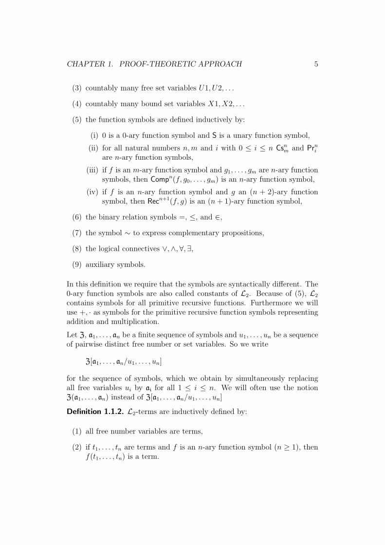
Definition 1.1.1. Let L2 denote the language of second order arithmeticwhich contains the following symbols:

(1) countably many free number variables u1, u2, . . .

(2) countably many bound number variables x1, x2, . . .

4

CHAPTER 1. PROOF-THEORETIC APPROACH 5

(3) countably many free set variables U1, U2, . . .

(4) countably many bound set variables X1, X2, . . .

(5) the function symbols are defined inductively by:

(i) 0 is a 0-ary function symbol and S is a unary function symbol,

(ii) for all natural numbers n,m and i with 0 ≤ i ≤ n Csnm and Prni

are n-ary function symbols,

(iii) if f is an m-ary function symbol and g1, . . . , gm are n-ary functionsymbols, then Compn(f, g0, . . . , gm) is an n-ary function symbol,

(iv) if f is an n-ary function symbol and g an (n + 2)-ary functionsymbol, then Recn+1(f, g) is an (n + 1)-ary function symbol,

(6) the binary relation symbols =, ≤, and ∈,

(7) the symbol ∼ to express complementary propositions,

(8) the logical connectives ∨,∧,∀,∃,

(9) auxiliary symbols.

In this definition we require that the symbols are syntactically different. The0-ary function symbols are also called constants of L2. Because of (5), L2

contains symbols for all primitive recursive functions. Furthermore we willuse +, · as symbols for the primitive recursive function symbols representingaddition and multiplication.

Let Z, a1, . . . , an be a finite sequence of symbols and u1, . . . , un be a sequenceof pairwise distinct free number or set variables. So we write

Z[a1, . . . , an/u1, . . . , un]

for the sequence of symbols, which we obtain by simultaneously replacingall free variables ui by ai for all 1 ≤ i ≤ n. We will often use the notionZ(a1, . . . , an) instead of Z[a1, . . . , an/u1, . . . , un]

Definition 1.1.2. L2-terms are inductively defined by:

(1) all free number variables are terms,

(2) if t1, . . . , tn are terms and f is an n-ary function symbol (n ≥ 1), thenf(t1, . . . , tn) is a term.


Numerals n for all natural numbers n are variable-free terms, defined byn :≡ S(. . . S(0) . . .) where S occurs n-times. They are used to representnatural numbers in L2.

The positive atomic formulas of L2 are expressions of the form t1 = t2, t1 ≤ t2and t1 ∈ U where t1, t2 are terms, and U is a set variable. The negative atomicformulas of L2 are expressions of the form ∼R where R is a positive atomicformula.

Literals are positive or negative atomic formulas.

Definition 1.1.3. L2-formulas are defined inductively by:

(1) every literal is a formula,

(2) if A, B are formulas, so are (A ∧B) and (A ∨B),

(3) if A is a formula, u a free number variable and x a bound numbervariable, which does not occur in A, then ∃xA[x/u] and ∀xA[x/u] areformulas,

(4) if A is a formula, U a free set variable and X a bound set variable, whichdoes not occur in A, then ∃XA[X/U ] and ∀XA[X/U ] are formulas.

By FV(t), FV(A) or FV(Γ) we denote the set of free variables which occurin the term t, in the formula A or the set of formulas Γ respectively. A termor formula is called closed or variable-free if FV(t) = ∅ resp. FV(A) = ∅.Closed formulas are often called sentences.

Definition 1.1.4 (Negation). The negation ¬A of a formula A is definedinductively by:

(1) if A is a positive atomic formula, then ¬A :≡ ∼A,

(2) if A ≡ ∼B and B positive atomic, then ¬A :≡ B,

(3) if A ≡ (B ∨ C), then ¬A :≡ (¬B ∧ ¬C),

(4) if A ≡ (B ∧ C), then ¬A :≡ (¬B ∨ ¬C),

(5) if A ≡ ∃xB[x/u], then ¬A :≡ ∀x¬B[x/u],

(6) if A ≡ ∀xB[x/u], then ¬A :≡ ∃x¬B[x/u],

(5) if A ≡ ∃XB[X/U ], then ¬A :≡ ∀X¬B[X/U ],


(6) if A ≡ ∀XB[X/U ], then ¬A :≡ ∃X¬B[X/U ].

The logical implication (A → B), logical equivalence (A ↔ B) and the binaryrelations <, 6= are introduced as abbreviations:

(A → B) :≡ (¬A ∨B) (A ↔ B) :≡ (A → B) ∧ (B → A)

(x 6= y) :≡ ¬(x = y) (x < y) :≡ (x ≤ y ∧ x 6= y)

As we will deal a lot with bounded formulas we introduce the followingabbreviations which we will use very often.

(1) (∀x ≤ t)A(x) :≡ ∀x(x ≤ t → A(x))

(2) (∃x ≤ s)A(x) :≡ ∃x(x ≤ s ∧ A(x))

Further we will use the vector notion ~z for finite sequences z1, . . . , zn. Thearity will always be clear from the context.

1.1.2 Arithmetical hierarchy and asymmetric translation

The quantifiers (∀x ≤ t) and (∃x ≤ s) are called bounded quantifiers. By∆0

0 = Σ00 = Π0

0 we denote the smallest collection of formulas generated fromliterals by means of conjunction, disjunction and bounded number quantifi-cation. ∆0

0-formulas may contain free set and free number variables, theso-called parameters.

The arithmetical hierarchy is inductively defined by:

(1) A is Σ01 if A ≡ ∃xB for a ∆0

0-formula B or A is ∆00,

A is Π01 if A ≡ ∀xB for a ∆0

0-formula B or A is ∆00.

(2) A is Σ0n+1 if A ≡ ∃xB for a Π0

n-formula B or A is Σ0n,

A is Π0n+1 if A ≡ ∀xB for a Σ0

n-formula B or A is Π0n+1.

Furthermore the collection of strict Π11- and strict Σ1

1-formulas will be of acertain interest in the sequel.

Definition 1.1.5 (s-Π11/s-Σ

11-formulas).

By s-Π11 we denote the smallest collection of formulas which are generated

from literals by means of ∧,∨,∃x ≤ t,∀x ≤ s, ∀X and ∃x.By s-Σ1

1 we denote the smallest collection of formulas which are generatedfrom literals by means of ∧,∨,∃x ≤ t,∀x ≤ s, ∃X and ∀x.


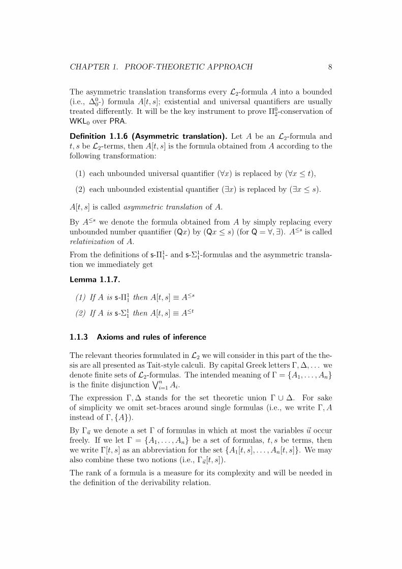
The asymmetric translation transforms every L2-formula A into a bounded(i.e., ∆0

0-) formula A[t, s]; existential and universal quantifiers are usuallytreated differently. It will be the key instrument to prove Π0

2-conservation ofWKL0 over PRA.

Definition 1.1.6 (Asymmetric translation). Let A be an L2-formula andt, s be L2-terms, then A[t, s] is the formula obtained from A according to thefollowing transformation:

(1) each unbounded universal quantifier (∀x) is replaced by (∀x ≤ t),

(2) each unbounded existential quantifier (∃x) is replaced by (∃x ≤ s).

A[t, s] is called asymmetric translation of A.

By A≤s we denote the formula obtained from A by simply replacing everyunbounded number quantifier (Qx) by (Qx ≤ s) (for Q = ∀,∃). A≤s is calledrelativization of A.

From the definitions of s-Π11- and s-Σ1

1-formulas and the asymmetric transla-tion we immediately get

Lemma 1.1.7.

(1) If A is s-Π11 then A[t, s] ≡ A≤s

(2) If A is s-Σ11 then A[t, s] ≡ A≤t

1.1.3 Axioms and rules of inference

The relevant theories formulated in L2 we will consider in this part of the the-sis are all presented as Tait-style calculi. By capital Greek letters Γ, ∆, . . . wedenote finite sets of L2-formulas. The intended meaning of Γ = {A1, . . . , An}is the finite disjunction

∨ni=1 Ai.

The expression Γ, ∆ stands for the set theoretic union Γ ∪ ∆. For sakeof simplicity we omit set-braces around single formulas (i.e., we write Γ, Ainstead of Γ, {A}).By Γ~u we denote a set Γ of formulas in which at most the variables ~u occurfreely. If we let Γ = {A1, . . . , An} be a set of formulas, t, s be terms, thenwe write Γ[t, s] as an abbreviation for the set {A1[t, s], . . . , An[t, s]}. We mayalso combine these two notions (i.e., Γ~u[t, s]).

The rank of a formula is a measure for its complexity and will be needed inthe definition of the derivability relation.


Definition 1.1.8 (Rank). The rank rk(A) of a formula A is defined by

(1) rk(A) = 0, if A is s-Π11 or s-Σ1

1,

(2) otherwise the rank is:

(i) rk(A ◦B) = max{rk(A), rk(B)}+ 1, if ◦ = ∧,∨,

(ii) rk(QxA(x)) = rk(A(u)) + 1, if Q = ∀,∃,(iii) rk(QXA(X)) = rk(A(U)) + 1, if Q = ∀,∃.

The following definition describes the axioms and rules of inference thatare present in all theories T we will consider. The mathematical rules ofinference and axioms are theory-dependent; this is: a theory consists of someadditional mathematical rules of inference (or axioms) which make up thetheory. Examples of the latter are: induction and comprehension rules forspecific collections of formulas. In the following two sections we define thetheories we will make use of.

Definition 1.1.9. The axioms of theories T formulated in L2 consist of thesubstitution closure of the following sets:

(A.1) Logical Axioms.

Γ, u = uΓ,¬u = v,¬A(u), A(v) (A atomic)Γ,¬A, A (A atomic).

(A.2) Axioms for primitive recursion.

Γ,¬S(u) = 0 Γ,¬S(u) = S(v), u = vΓ,¬u < 0 Γ,¬u < S(v), u < v, u = vΓ, u < v, u < S(v), u = v Γ,¬u < v, u < S(v)Γ¬u = v, u < v Γ, u < v, u = v, v < uΓ, Csn

m(u1, . . . , un) = m Γ, Prni (u1, . . . , un) = ui

Γ, Compn(f, g1, . . . , gn)(~u) = f(g1(~u), . . . , gn(~u))Γ, Recn+1(f, g)(~u, 0) = f(~u)Γ, Recn+1(f, g)(~u, S(v)) = g(u, v, Recn+1(f, g)(~u, v))

The logical rules of inference are given by.


(R.1) Logical Rules

Γ, A Γ, B

Γ, A ∧B(∧)

Γ, A

Γ, A ∨B(∨1)

Γ, B

Γ, A ∨B(∨2)

Γ, A(u)

Γ,∀xA(x)(∀0), provided u is not a free variable in Γ,∀xA(x)

Γ, A(t)

Γ,∃xA(x)(∃0), where t is an arbitrary term.

Γ, A Γ,¬A

Γ(cut)

Γ, A(U)

Γ,∀XA(X)(∀1), provided U is not a free variable in Γ,∀XA(X)

Γ, A(U)

Γ,∃XA(X)(∃1)

1.1.4 Theories RCA0 and ∆0-CA

In this section we will define two second-order theories which will be im-portant: RCA0 with recursive comprehension (RCA stands for RecursiveComprehension Axiom, the zero indicates restricted induction), and theweaker theory ∆0-CA in which we will interpret (s-Π1

1) + RCA0 asymmet-rically. Both theories are weak subsystems of ACA0.

Definition 1.1.10 (RCA0). The theory RCA0 is formulated in L2 and containsthe axioms and logical rules of inference given in definition 1.1.9 and thefollowing mathematical rules:

(R.2) Mathematical Rules.For any Σ0

1-formula A(u):

Γ, A(0) Γ,∀x(A(x) → A(S(x))

Γ, A(t)(Σ0

1-IND), t any term

For any Σ01-formula A(u) and Π0

1-formula B(u):

Γ,∀x(A(x) → B(x)) Γ,∀x(B(x) → A(x))

Γ,∃X[∀x(x ∈ X → B(x)) ∧ ∀x(A(x) → x ∈ X)](∆0

1-CR)

∆01-comprehension is often also called recursive comprehension, since a set is

recursive iff itself and its complement are recursively enumerable and recur-sively enumerable sets correspond to Σ1-definable sets in N.


In the literature about RCA0 or reverse mathematics, such as Simpson [10], wewill find ∆0

1-comprehension and Σ01-induction formulated as axiom-schemes;

these axioms are logical consequences of the rules presented here (becausewe have formulated them with side-formulas).

Definition 1.1.11 (∆0-CA). The theory ∆0-CA is formulated in L2 and con-tains the axioms and logical rules of inference given in definition 1.1.9 andthe following mathematical axioms and rules:

(A.2) Axiom for ∆00-comprehension.

For any ∆00-formula A(u):

Γ,∃X∀x(x ∈ X ↔ A(x)) (∆00-CA)

(R.2) Mathematical Rules.For any ∆0

0-formula A(u):

Γ, A(0) Γ,∀x(A(x) → A(S(x))

Γ, A(t)(∆0

0-IND), t any term

1.2 WKL: Weak Konig’s lemma

In ordinary mathematics weak Konig’s Lemma is stated as follows:

Weak Konig’s Lemma.1 Given an infinite binary tree T , there exists aninfinite path P through the tree T .

We need a formulation of “binary tree” and “path” in our second orderarithmetic. Since our language L2 contains symbols for all primitive recursivefunctions, there is a symbol of a primitive recursive function that maps finitesequences x1, . . . , xn of natural numbers to the so-called sequence number〈x1, . . . , xn〉 which is a standard result from basic recursion theory (cf. forexample Jager [7]). On the other hand we can also find a primitive recursive“decoding” function (·)i with the property (〈x1, . . . , xn〉)i = xi and a lengthfunction lh(·) defined on sequence numbers. Furthermore we can define aprimitive recursive predicate Seq(x) which holds iff x is a sequence number.

Now we are able to define a binary relation ⊆ on the set of all sequencenumbers stating that u is a subsequence of v, u ⊆ v, formally:

u ⊆ v :≡ Seq(u) ∧ Seq(v) ∧ ∀x ≤ lh(u)[(u)x = (v)x]

1which is named after the Hungarian mathematician Denes Konig (1884–1944)


We require all sequences, that build up the tree to be binary (i.e., to consistonly of 0 and 1). So we define an additional unary predicate Seq2(·), ensuringthat a given sequence s consists only of 0’s and 1’s:

Seq2(s) ≡ Seq(s) ∧ ∀x ≤ lh(s)[(s)x = 0 ∨ (s)x = 1]

An infinite binary tree is therefore a set consisting of 0-1-sequence numbersof arbitrary length that are closed under initial subsequences.

Definition 1.2.1. Let U be a set of sequence-numbers. U defines an infi-nite binary tree, if U consists only of 0-1 sequence numbers, is closed undersubsequences and contains sequences of arbitrary length; formally:

Tree∞(U) :≡ ∀x(x ∈ U → Seq2(x))∧∀x∀y(x ∈ U ∧ y ⊆ x → y ∈ U)∧∀x∃y ≤ 〈1〉(x)(y ∈ U ∧ lh(y) = x)

where 〈1〉 denotes the unary primitive-recursive function symbol with theproperty 〈1〉(x) = 〈1, . . . , 1︸︷︷︸

x-times

〉.

A path is an infinite tree linearly ordered with respect to the subsequencerelation:

Path∞(U) :≡ Tree∞(U) ∧ ∀x∀y(x ∈ U ∧ y ∈ U → x ⊆ y ∨ y ⊆ x)

We remark that RCA0 6` (WKL), as the standard model M = (ω,REC,≤M,SM, . . . ) of RCA0 is a not model of (WKL). There exist infinite recursive treeswith no recursive paths (e.g., Kleene-Tree).

1.2.1 Theory WKL0 and strict Π11-reflection

In this section we formally define the theory WKL0 which consists of thesame axioms and rules as RCA0 plus weak Konig’s lemma principle (WKL).We will not directly work within WKL0, but we define an additional theorybased on RCA0 with the strict Π1

1-reflection rule (s-Π11) which will prove weak

Konig’s lemma, so we can embed WKL0 in this theory. Strict Π11-reflection is

an important reflection principle which is equivalent to weak Konig’s lemma.A predicate P on N is strict Π1

1 iff it is recursively enumerable. For more in-formation and details on s-Π1

1-reflection and s-Π11-sets we refer to Barwise [1].

Definition 1.2.2. The theory WKL0 is formulated in L2 and contains theaxioms and logical rules of inference given in definition 1.1.9 and the followingmathematical rules:



1-formula A(u):

Γ, A(0) Γ,∀x(A(x) → A(S(x))

Γ, A(t)(Σ0

1-IND), t any term


1-formula B(u):

Γ,∀x(A(x) → B(x)) Γ,∀x(B(x) → A(x))

Γ,∃X[∀x(x ∈ X → B(x)) ∧ ∀x(A(x) → x ∈ X)](∆0

1-CR)

Γ, Tree∞(U)

Γ,∃X[Path∞(X) ∧ ∀x(x ∈ X → x ∈ U)](WKL)

Definition 1.2.3. The theory s-RCA0 is formulated in L2 and contains theaxioms and logical rules of inference given in definition 1.1.9 and the followingmathematical rules:


1-formula A(u):

Γ, A(0) Γ,∀x(A(x) → A(S(x))

Γ, A(t)(Σ0

1-IND), t any term


1-formula B(u):

Γ,∀x(A(x) → B(x)) Γ,∀x(B(x) → A(x))

Γ,∃X[∀x(x ∈ X → B(x)) ∧ ∀x(A(x) → x ∈ X)](∆0

1-CR)

For any s-Π11-formula A

Γ, A

Γ,∃xA≤x(s-Π1

1)

According to this definition, s-RCA0 equals RCA0 + (s-Π11) in which we will

embed WKL0.

1.3 Derivability relation and useful results from proof-theory

In this section we will state the definition of the derivability relation in ourTait-calculus and some basic results which come from ordinary proof-theorythat we will be often using. For further information on proof theory we referto Schutte [8], Girard [4] or Takeuti [11].

Definition 1.3.1 (Derivability). The derivability relation T mn

Γ (m, n ∈ ω)for theories T formulated in L2 is inductively defined by the clauses:


(1) If Γ is an axiom, T mn

Γ for every m, n.

(2) Assume that Γ is the conclusion from the premises Γi of a logical ormathematical rule, or of a cut of rank < n with T mi

nΓi (i < 3) and

mi < m. Then T mn

Γ.

T mn

Γ means that there exists a proof of Γ whose depth is bound by m andwhich contains only cuts of rank smaller than n.

Lemma 1.3.2 (Weakening). If s-RCA0mn

Γ and Γ ⊂ ∆, then s-RCA0mn

∆

Lemma 1.3.3. s-RCA0 ` Γ, A and s-RCA0 ` ∆,¬A imply s-RCA0 ` Γ, ∆.

Proof. Obvious.

Lemma 1.3.4 (Inversion).

(1) If s-RCA0mn

Γ, A1 ∧ A2 and rk(A1 ∧ A2) > 0 then s-RCA0mn

Γ, Ai

(i = 1, 2).

(2) If s-RCA0mn

Γ, A1 ∨A2 and rk(A1 ∨A2) > 0 then s-RCA0mn

Γ, A1, A2.

(3) If s-RCA0mn

Γ,∀xA(x) and rk(∀xA(x)) > 0 then s-RCA0mn

Γ, A(t)(t an individual term).

(4) If s-RCA0mn

Γ,∀XA(X) and rk(∀XA(X)) > 0 then s-RCA0mn

Γ, A(U).

Weak cut elimination gives us the information that any proof can be trans-lated into one using only formulas of rank < 1 in the cut rule, even thoughthe depth of the proof will increase. “Weak” in this context means that weonly eliminate cuts of rank ≥ 1. Since the principal formulas of conclusionsof mathematical rules are always s-Π1

1 or s-Σ11 and thus have a cut-rank of

zero, we do not eliminate these cuts. In the cut-elimination procedure wereplace cuts occuring in the proof by cuts with a smaller rank (which lets theproof-depth increase).

Further information on cut elimination can be found in Schwichtenberg [9],for instance.

Theorem 1.3.5 (Weak cut elimination). If s-RCA0 ` Γ, then s-RCA0k1

Γfor some k ∈ ω.

The following lemma is very helpful in the proceeding; it is so-to-speak thetechnical tool to handle the asymmetric interpretation of the rules of inferencequite easily. As sets of formulas are interpreted as the disjunction of its


members, it is not required to apply it to all members of the set. Thus wemay leave some formulas of a set untouched if we wish so.

Lemma 1.3.6 (Persistence). Let Γ ∪ {A} be a set of L2-formulas.

(1) ∆0-CA ` ¬t′ ≤ t, s ≤ s′,¬A[t, s], A[t′, s′]

(2) If A is s-Π11, then A[t, s] ≡ A≤s and ∆0-CA ` ¬s ≤ t,¬A≤s, A≤t

(3) If A is s-Σ11, then A[t, s] ≡ A≤t and ∆0-CA ` ¬t ≤ s,¬A≤s, A≤t

where ¬A[t, s] is an abbreviation for ¬(A[t, s]).

Proof. (2) and (3) are easy consequences of (1) and lemma 1.1.7. We prove(1) on the build-up of formulas:

Let A be atomic, then A ≡ A[t, s] ≡ A[t′, s′] and ¬t′ ≤ t,¬s ≤ s′,¬A[t, s], A[t′, s′]is a logical axiom by definition 1.1.9 (A.1).

A ≡ B ∧ C: By induction hypothesis we have

¬t′ ≤ t,¬s ≤ s′,¬A[t, s], A[t′, s′] and ¬t′ ≤ t,¬s ≤ s′,¬B[t, s], B[t′, s′]

Applying (∨i) to both sets of formulas yields

¬t′ ≤ t,¬s ≤ s′,¬A[t, s] ∨ ¬B[t, s], A[t′, s′]

¬t′ ≤ t,¬s ≤ s′,¬A[t, s] ∨ ¬B[t, s], B[t′, s′]

A final (∧) between these two lines gives

¬t′ ≤ t,¬s ≤ s′,¬(A[t, s] ∧B[t, s]), A[t′, s′] ∧B[t′, s′]

A ≡ B ∨ C: analogously to the previous case.

A ≡ ∀xB: Let v 6∈ FV(¬t′ ≤ t,¬s ≤ s′,¬B[t, s], B[t′, s′]). Then ¬t′ ≤ t,¬s ≤ s′, v ≤ t,¬v ≤ t′ is provable, since ≤ is transitive. Hence by weakening:

¬t′ ≤ t,¬s ≤ s′, v ≤ t,¬v ≤ t′, B[t′, s′] (1.3.1)

By induction hypothesis we are allowed to assume:

¬t′ ≤ t,¬s ≤ s′,¬B[t, s], B[t′, s′]

using weakening on the previous sequent leads to:

¬t′ ≤ t,¬s ≤ s′,¬B[t, s], B[t′, s′],¬v ≤ t′ (1.3.2)


Applying (∧) between (1.3.1) and (1.3.2) yields:

¬t′ ≤ t,¬s ≤ s′, v ≤ t ∧ ¬B[t, s], B[t′, s′],¬v ≤ t′ (1.3.3)

By (∃0)-introduction and using (∨2) we obtain from the preceding lines:

¬t′ ≤ t,¬s ≤ s′,¬∀x ≤ tB[t, s],¬v ≤ t′ ∨B[t′, s′]

A last application of (∀0) is needed to get to the desired result

¬t′ ≤ t,¬s ≤ s′,¬∀x ≤ tB[t, s],∀x ≤ tB[t′, s′]

A ≡ ∃xB: This case is similar to (∀); assume v 6∈ FV(¬t′ ≤ t,¬s ≤ s′, B[t, s],B[t′, s′]) and by transitivity of ≤, ¬s ≤ s′,¬v ≤ s, v ≤ s′ is provable. Hence,by weakening:

¬s ≤ s′,¬v ≤ s, v ≤ s′,¬B[t, s] (1.3.4)

By induction hypothesis we are allowed to assume:

¬t′ ≤ t,¬s ≤ s′,¬B[t, s], B[t′, s′]

using weakening on the previous sequent leads to:

¬t′ ≤ t,¬s ≤ s′,¬B[t, s], B[t′, s′],¬v ≤ s (1.3.5)

An application of (∧) between the sequents in (1.3.4) and (1.3.5) leads to

¬t′ ≤ t,¬s ≤ s′,¬v ≤ s,¬B[t, s], v ≤ s′ ∧B[t′, s′]

By (∃0)-introduction and using (∨1) we obtain from the preceding sequent:

¬t′ ≤ t,¬s ≤ s′,¬v ≤ s ∨ ¬B[t, s],∃x ≤ s′B[t′, s′]

Eventually we apply (∀0) and get the required result:

¬t′ ≤ t,¬s ≤ s′,∃x ≤ sB[t, s],∃x ≤ s′B[t′, s′]

A ≡ ∀XB(X), A ≡ ∃XB(X): these cases are obvious.


1.4 Asymmetric interpretation theorem

The following proposition shows the already mentioned fact that RCA0 +(s-Π1

1) proves weak Konig’s lemma. So it is sufficient to show all subsequentresults for s-RCA0 and henceforth it applies to WKL0 as well. The asymmetricinterpretation of s-RCA0 is more elegant than the one for WKL0 even though adirect asymmetric interpretation of WKL0 could be accomplished, as Cantinishows in [2] for his bounded arithmetic.

Proposition 1.4.1. RCA0 and s-Π11-reflection imply weak Konig’s lemma:

RCA0 + (s-Π11) ` (WKL).

Proof. We show the contra positive, i.e., RCA0 + (s-Π11) proves

∀Y [Path∞(Y ) → ∃w(w ∈ Y ∧ ¬w ∈ U)] → ¬Tree∞(U).

Therefore we assume

∀Y [Path∞(Y ) → ∃w(w ∈ Y ∧ ¬w ∈ U)] (1.4.1)

∀x∀y(Seq2(x) ∧ x ∈ U ∧ y ⊆ x → y ∈ U) (1.4.2)

∀x(x ∈ U → Seq2(x)) (1.4.3)

By the strict Π11-reflection rule we obtain a bound b such that

∀Y [Path∞≤b(Y ) → ∃w ≤ b(w ∈ Y ∧ ¬w ∈ U)].

We claim that the tree defined by U is finite and all its paths have length< b, i.e.,

∀x(Seq2(x) ∧ lh(x) = b → ¬x ∈ U) (1.4.4)

Let z be arbitrary with lh(z) = b ∧ Seq2(z) then by ∆01-comprehension there

exists the set X(z) := {u : u ⊆ z}. Then X(z) satisfies

(∀x ≤ b)[x ∈ X → Seq2(x)] (1.4.5)

(∀x ≤ b)(∀y ≤ b)[x ∈ X(z) ∧ y ⊆ x → y ∈ X(z)] (1.4.6)

(∀x ≤ b)(∃y ≤ 〈1〉(x))[y ∈ X(z) ∧ lh(y) = x] (1.4.7)

(∀x ≤ b)(∀y ≤ b)[x ∈ X(z) ∧ y ∈ X(z) → x ⊆ y ∨ y ⊆ x] (1.4.8)

Hence, Path∞≤b(X(z)) holds and thus, since

Path∞(X(z)) → ∃w ≤ b(w ∈ X(z) ∧ ¬w ∈ U),

we conclude there exists w such that w ⊆ z∧w ∈ X(z)∧¬w ∈ U with length≤ b. By (1.4.2) we conclude ¬z ∈ U , the verification of (1.4.4).


On our way to the Π02-conservativity we prove the asymmetric interpretation

theorem of s-RCA0 in ∆0-CA. Based on this, we will show the conservativ-ity. If we apply the transformation of asymmetric translation to any formulaprovable in s-RCA0 (and thus also in WKL0) we will get a bounded formulawhich will be provable in the weaker system ∆0-CA. The bound of an exis-tential quantifier depends on the given bound of the universal quantifier.

Theorem 1.4.2 (Asymmetric interpretation). Let s-RCA0k1

Γ~z. Then onecan find a unary primitive recursive function symbol g of L2 such that, prov-ably in ∆0-CA:

(1) ∀x∀~z(~z ≤ x →∨

Γ~z[x, g(x)]);

(2) ∀x(x ≤ g(x))

Proof. We prove the claim by induction on the depth of the derivation. Asthe logical axioms and axioms for primitive recursion are atomic, we may letg(u) = u and thus the claim holds.

(∧): The (∧)-rule applies if we can prove Γ, A and Γ, B in s-RCA0, thenby induction hypothesis we may assume that ∆0-CA proves the asymmetrictranslation of these two premises of (∧) and thus we have u ≤ gi(u) (i = 1, 2)and

¬~z ≤ u, Γ~z[u, g1(u)], A[u, g1(u)] (1.4.9)

¬~z ≤ u, Γ~z[u, g2(u)], B[u, g2(u)] (1.4.10)

Define g(u) := g1(u)+g2(u), then clearly u ≤ g(u) and by persistence (gi(u) ≤g(u) for i = 1, 2) we get:

¬~z ≤ u, Γ~z[u, g(u)], A[u, g(u)] (1.4.11)

¬~z ≤ u, Γ~z[u, g(u)], B[u, g(u)] (1.4.12)

Applying (∧) to (1.4.11) and (1.4.12) yields the result.

(∨1,2): analogously to (∧)

(∀0): Then Γ~z = ∆~z,∀xA(x) and thus we have for some v 6∈ FV(Γ~z) andsome k0 < k

s-RCA0k0

1Γ~z, A(v)

By the induction hypothesis we have provably in ∆0-CA

¬v, ~z ≤ u, Γ~z[u, g0(u)], A[u, g0(u)](v)


for some term g0(u) such that u ≤ g0(u). We define g(u) = g0(u) and hence

¬v, ~z ≤ u, Γ~z[u, g(u)], A[u, g(u)](v)

Since v 6∈ FV(Γ~z) we may apply (∀0) and obtain:

¬~z ≤ u, Γ~z[u, g(u)],∀x ≤ uA[u, g(u)](x)

(∃0): Then Γ~z = ∆~z,∃xA(x) and s-RCA0k1

Γ~z, A(s) for some k ∈ ω andsome term s = s(~z). By induction hypothesis, we have, provably in ∆0-CA,u ≤ g(u) and under the assumption ~z ≤ u

Γ~z[u, g(u)], A[u, g(u)](s)

Since every primitive-recursive function f can be majorized by a mono-tone primitive-recursive one (e.g., a branch of the Ackermann function),we can find a term s′(~z) which is monotone with respect to ≤, such thats(~z) ≤ s′(~z) ≤ s′(u, . . . , u). Then we choose h(u) := g(u) + s′(u, . . . , u).Obviously s(~z), g(u) ≤ h(u). The persistence lemma and (∃0) imply therequired conclusion.

(s-Π11): Let A be s-Π1

1 i.e., A[t, s] ≡ A≤s, and assume ~z ≤ u; then by inductionhypothesis we may assume

Γ~z[u, g(u)], A≤g(u).

Choose h(u) := g(u); with an application of (∧) we get

Γ~z[u, g(u)], g(u) ≤ h(u) ∧ A≤g(u) (1.4.13)

Applying (∃0) yields

Γ~z[u, h(u)],∃x(x ≤ h(u) ∧ A≤x) (1.4.14)

≡ Γ~z[u, h(u)],∃x ≤ h(u)A≤x (1.4.15)

(∆01-CR): By induction hypothesis we may assume that ∆0-CA proves the

asymmetric translation of the two premises of (∆01-CR) and thus there exist

terms g0(u), g1(u) with u ≤ g0(u), g1(u) such that under the assumption~z ≤ u

Γ~z[u, g0(u)],∀y ≤ u[∃x ≤ uA(x, y) → ∀x ≤ uB(x, y)] (1.4.16)

Γ~z[u, g1(u)],∀y ≤ u[∀x ≤ g1(u)B(x, y) → ∃x ≤ g1(u)A(x, y)] (1.4.17)


If we choose g(u) := g0(g1(u)) and let u = g1(u) then (1.4.16) implies

Γ~z[g1(u), g(u)],∀y ≤ g1(u)[∃x ≤ g1(u)A(x, y) →∀x ≤ g1(u)B(x, y)]

(1.4.18)

whence by persistence we get from (1.4.17) and (1.4.18)

Γ~z[u, g(u)],∀y ≤ u[∃x ≤ g1(u)A(x, y) → ∀x ≤ g1(u)B(x, y)] (1.4.19)

Γ~z[u, g(u)],∀y ≤ u[∀x ≤ g1(u)B(x, y) → ∃x ≤ g1(u)A(x, y)] (1.4.20)

As w ≤ u ∧ ∃x ≤ g1(u)A(x, w) is a ∆00-formula, we obtain by the (∆0

0-CA)axiom the following sequent

Γ~z[u, g(u)],∃X∀y[y ∈ X ↔ (y ≤ u ∧ ∃x ≤ g1(u)A(x, y))] (1.4.21)

Hence by logic

Γ~z[u, g(u)],∃X[∀y(y ∈ X → (y ≤ u ∧ ∃x ≤ g1(u)A(x, y))∧∀y((y ≤ u ∧ ∃x ≤ g1(u)A(x, y)) → y ∈ X)]

(1.4.22)

Then from (1.4.22) together with (1.4.19) we obtain by logic

Γ~z[u, g(u)],∃X[∀y(y ∈ X → (y ≤ u ∧ ∀x ≤ g1(u)B(x, y))∧∀y((y ≤ u ∧ ∃x ≤ g1(u)A(x, y)) → y ∈ X)]

(1.4.23)

A last application of persistence and some logic on the preceding sequentyields the asymmetric interpretation of the conclusion of (∆0

1-CR)

Γ~z[u, g(u)],∃X[∀y ≤ u(y ∈ X → ∀x ≤ uB(x, y))∧∀y ≤ u(∃x ≤ uA(x, y) → y ∈ X)]

(1.4.24)

Surprisingly we only need one asymmetrically interpreted premise of (∆01-CR).

At a first look this may seem strange, since if we only take ∀x(A(x) → B(x))(A(u) is Σ0

1, B(u) is Π01) from the conjunction in the premise of ∆0

1-CA, wecan prove the existence of some separable sets, which would not be possiblein RCA0. But it is a consequence of (WKL) and hence we do not get toomuch comprehension.

(Σ01-IND): By induction hypothesis there exist terms g0(u), g1(u) with u ≤

g0(u), g1(u) such that ∆0-CA proves the asymmetrically translated premisesof (Σ0

1-IND):

Γ~z[u, g0(u)],∃x ≤ g0(u)A(x, 0) (1.4.25)

Γ~z[u, g1(u)],∀y ≤ u[∃x ≤ uA(x, y) → ∃x ≤ g1(u)A(x, S(y))] (1.4.26)


By primitive recursion, we define a term f as f(u, 0) = g0(u) and f(u, S(v)) =g1(f(u, v)) + 1. By ∆0

0-induction on v we will prove

Γ~z[u, f(u, v)],∃x ≤ f(u, v)A(x, v). (1.4.27)

By definition of f and persistence we have

Γ~z[u, f(u, v)],∃x ≤ f(u, 0)A(x, 0) (1.4.28)

Now we assume

Γ~z[u, f(u, v)],∃x ≤ f(u, v)A(x, v) (1.4.29)

If we let u = f(u, v), then we obtain from (1.4.26) using persistence (u ≤f(u, v) on (1.4.26))

Γ~z[u, f(u, S(v))],∀y ≤ f(u, v)[∃x ≤ f(u, v)A(x, y) →∃x ≤ f(u, S(v))A(x, S(y))]

(1.4.30)

Then by (∀0)-inversion we obtain

Γ~z[u, f(u, S(v))], v ≤ f(u, v)[∃x ≤ f(u, v)A(x, v) →∃x ≤ f(u, S(v))A(x, S(v))]

(1.4.31)

Using persistence (f(u, v) ≤ f(u, S(v))) on (1.4.29) we get

Γ~z[u, f(u, S(v))],∃x ≤ f(u, S(v))A(x, S(v)) (1.4.32)

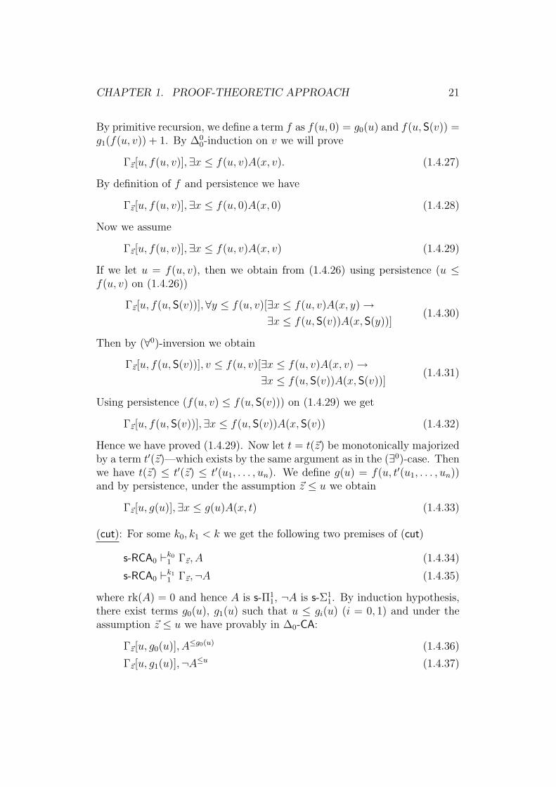
Hence we have proved (1.4.29). Now let t = t(~z) be monotonically majorizedby a term t′(~z)—which exists by the same argument as in the (∃0)-case. Thenwe have t(~z) ≤ t′(~z) ≤ t′(u1, . . . , un). We define g(u) = f(u, t′(u1, . . . , un))and by persistence, under the assumption ~z ≤ u we obtain

Γ~z[u, g(u)],∃x ≤ g(u)A(x, t) (1.4.33)

(cut): For some k0, k1 < k we get the following two premises of (cut)

s-RCA0 `k01 Γ~z, A (1.4.34)

s-RCA0 `k11 Γ~z,¬A (1.4.35)

where rk(A) = 0 and hence A is s-Π11, ¬A is s-Σ1

1. By induction hypothesis,there exist terms g0(u), g1(u) such that u ≤ gi(u) (i = 0, 1) and under theassumption ~z ≤ u we have provably in ∆0-CA:

Γ~z[u, g0(u)], A≤g0(u) (1.4.36)

Γ~z[u, g1(u)],¬A≤u (1.4.37)


Define g(u) := g1(g0(u)) and we have provably in ∆0-CA, u ≤ g(u). Letu := g0(u), then from (1.4.37) we obtain

Γ~z[g0(u), g(u)],¬A≤g0(u) (1.4.38)

Now using persistence, (1.4.36) and (1.4.38) yield

Γ~z[u, g(u)], A≤g0(u) (1.4.39)

Γ~z[u, g(u)],¬A≤g0(u) (1.4.40)

A cut between these last two sequents gives the desired result.

Using the above theorem we will almost immediately get the Π02-conservation

result of WKL0 over ∆0-CA.

Corollary 1.4.3 (Conservation). WKL0 is a conservative extension of ∆0-CAfor Π0

2-sentences, i.e. if A is Π02 and WKL0 ` A then ∆0-CA ` A.

Proof. Let A(u, v) be ∆00 and WKL0 ` ∀x ∃yA(x, y). By proposition 1.4.1 and

the asymmetric interpretation theorem ∆0-CA ` (∀x ≤ u)(∃y ≤ f(u))A(x, y)for an appropriate term f . By (∀0)- and (∨i)-inversion we conclude

¬u ≤ u, ∃y ≤ f(u)A(u, y). (1.4.41)

A cut between (1.4.41) and the axiom u ≤ u, ∃y ≤ f(u)A(u, y) yields

∃y ≤ f(u)A(u, y)

By logic we deduce ∃yA(u, y) from ∃y ≤ f(u)A(u, y) and an application of(∀0) finally yields ∀x∃yA(x, y).

Using the asymmetric interpretation of WKL0 in ∆0-CA it does not seem tobe possible to get a conservation result for a bigger collection of formulasthan Π0

2-formulas. It remains an open question if there exists a purely proof-theoretic method to obtain full conservation of WKL0 over ∆0-CA.

1.5 Π02-conservativity of WKL0 over PRA

Theoretically we could have interpreted WKL0 directly in RCA0 and thenproved the conservativity of RCA0 over PRA. In this thesis we have already


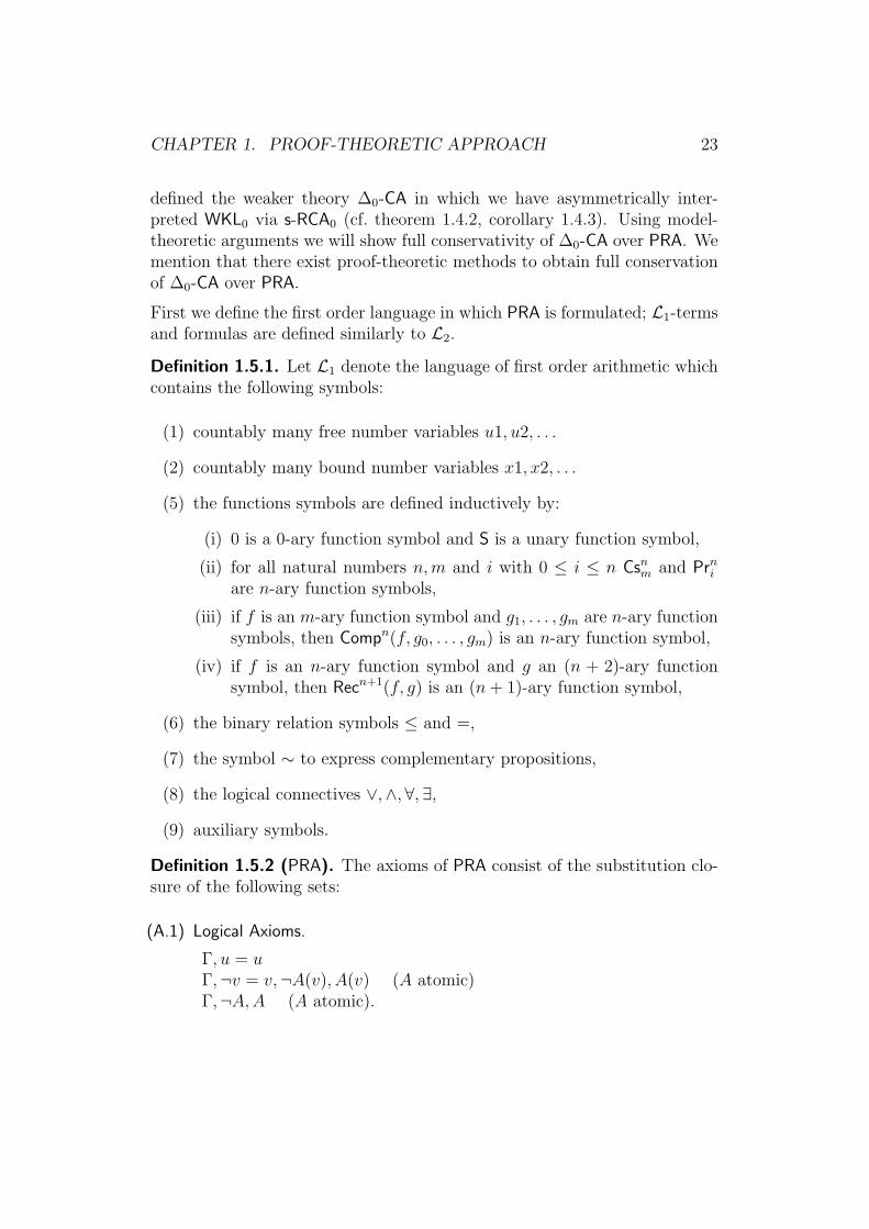
defined the weaker theory ∆0-CA in which we have asymmetrically inter-preted WKL0 via s-RCA0 (cf. theorem 1.4.2, corollary 1.4.3). Using model-theoretic arguments we will show full conservativity of ∆0-CA over PRA. Wemention that there exist proof-theoretic methods to obtain full conservationof ∆0-CA over PRA.

First we define the first order language in which PRA is formulated; L1-termsand formulas are defined similarly to L2.

Definition 1.5.1. Let L1 denote the language of first order arithmetic whichcontains the following symbols:

(1) countably many free number variables u1, u2, . . .

(2) countably many bound number variables x1, x2, . . .

(5) the functions symbols are defined inductively by:

(i) 0 is a 0-ary function symbol and S is a unary function symbol,

(ii) for all natural numbers n, m and i with 0 ≤ i ≤ n Csnm and Prni

are n-ary function symbols,

(iii) if f is an m-ary function symbol and g1, . . . , gm are n-ary functionsymbols, then Compn(f, g0, . . . , gm) is an n-ary function symbol,

(iv) if f is an n-ary function symbol and g an (n + 2)-ary functionsymbol, then Recn+1(f, g) is an (n + 1)-ary function symbol,

(6) the binary relation symbols ≤ and =,

(7) the symbol ∼ to express complementary propositions,

(8) the logical connectives ∨,∧,∀,∃,


Definition 1.5.2 (PRA). The axioms of PRA consist of the substitution clo-sure of the following sets:

(A.1) Logical Axioms.

Γ, u = uΓ,¬v = v,¬A(v), A(v) (A atomic)Γ,¬A, A (A atomic).


(A.2) Axioms for primitive recursion.

Γ,¬S(u) = 0 Γ,¬S(u) = S(v), u = vΓ,¬u < 0 Γ,¬u < S(v), u < v, u = vΓ, u < v, u < S(v), u = v Γ,¬u < v, u < S(v)Γ¬u = v, u < v Γ, u < v, u = v, v < uΓ, Csn

m(u1, . . . , un) = m Γ, Prni (u1, . . . , un) = ui

Γ, Compn(f, g1, . . . , gn)(~u) = f(g1(~u), . . . , gn(~u))Γ, Recn+1(f, g)(~u, 0) = f(~u)Γ, Recn+1(f, g)(~u, S(v)) = g(u, v, Recn+1(f, g)(~u, v))

The logical rules of inference are given by.

(R.1) Logical Rules

Γ, A Γ, B

Γ, A ∧B(∧)

Γ, A

Γ, A ∨B(∨1)

Γ, B

Γ, A ∨B(∨2)

Γ, A(u)

Γ,∀xA(x)(∀), provided u is not a free variable in Γ,∀xA(x)

Γ, A(t)

Γ,∃xA(x)(∃), where t is an arbitrary term.

Γ, A Γ,¬A

Γ(cut)

(R.2) Mathematical Rules.For any quantifier-free formula A(u):

Γ, A(0) Γ,∀x(A(x) → A(S(x))

Γ, A(t)(QF-IND), t any term

An arithmetical hierarchy can be defined analogously for L1; A is ∆0 if it isgenerated from literals by means of conjunctions, disjunction and boundedquantification. ∃xA is Σn+1 if A is Πn and ∀xA is Πn+1 if A is Σn.

It is a well-known result that PRA proves induction for the bigger collection ofbounded formulas. This is, for every bounded formula A there exists a quan-tifier-free formula B such that PRA ` A ↔ B and hence PRA ` (∆0-IND).

To prove conservativity of ∆0-CA over PRA it is sufficient to show that wecan extend every first-order model M of PRA to a second-order model M? of∆0-CA such that for any formula A in the language L1, M |= A ⇔M? |= A.This is because if we assume ∆0-CA ` A and PRA 6` A for any A in thelanguage L1 of PRA. By Godel completeness there exists a model M |= PRA


such that M 6|= A. As M? |= ∆0-CA we have consequently M? 6|= A andhence by soundness ∆0-CA 6` A, which contradicts our initial assumption.

Consider a model M of PRA

M = (M, +M, ·M, SM,≤M, . . .)

In order to extend M to a second-order model M? of ∆0-CA we have todefine the universe over which set variables will run:S ∈ SM if there exists a ∆0 L1-formula A(m,~n) with parameters ~n ∈ Msuch that S = {m ∈ M : M |= A(m,~n)}.

We claim that M? = (M,SM, +M, ·M, SM,≤M, . . .) is a model of ∆0-CA.The axioms (A.1) and (A.2) from definition 1.1.9 are clearly satisfied as theycoincide; we have to verify that M? satisfies ∆0

0-CA and ∆00-IND.

Let A be ∆00 in the language L2 with parameters from |M|∪SM? . Exhibiting

the parameters A ≡ A(u; X1, . . . , Xm, a1, . . . , ak). By definition of SM we canfind a formula Bi(tj) for every literal tj ∈ Xi such that tj ∈ Xi holds iff Bi(tj)holds. As the collection of ∆0

0 formula is closed under ∆00, we can replace

every literal tj ∈ Xi in A by the corresponding formula Bi(tj) and obtain aformula A such that M? |= A ↔ A. A is ∆0 and formulated in L1.

Assume A(u; X1, . . . , Xm, a1, . . . , ak) is ∆00, so we can find A(u) with the

only free variable u such that M |= A(u; X1, . . . , Xm, a1, . . . , ak) ↔ A(u).As A is ∆0, it defines a set X := {m ∈ M : A(m)} which is then inSM. So M? |= ∃X∀x(x ∈ X ↔ A(x)), and thus M? |= ∃X∀x(x ∈ X ↔A(x; X1, . . . , Xm, a1, . . . , ak)).

LetM? |= A(0)∧∀x(A(x) → A(S(x))) by replacing all set parameters in A byappropriate literals t ∈ Xi, we obtain an equivalent L1-formula A and henceM |= A(0) ∧ ∀x(A(x) → A(S(x))). As PRA ` ∆0-IND we have M |= A(v)and thus M? |= A(v) and eventually M? |= A(v).

So far we have just proved:

Lemma 1.5.3. ∆0-CA is conservative over PRA.

Composing corollary 1.4.3 and lemma 1.5.3 together we get our main resultin this section:

Theorem 1.5.4. WKL0 is Π02-conservative over PRA.


Using model-theoretic methods or the recursion-theoretic approach as pre-sented in the next part, we can prove the full conservation result of WKL0

over Σ1-PA. On the other hand, the proof-theoretic approach seems to memuch more intuitive than the recursive one.

The axiomatic method has many advantagesover honest work.

— BERTRAND RUSSEL

Recursion-theoretic Approach

In this chapter we will prove the full conservation result of WKL0 over Σ1-PA,following closely Hajek–Pudlak [6] resp. Hajek–Kucera [5]. The necessarydefinitions will be given, but some rather technical results will be cited only.

2.1 Logical Framework

In this part of the thesis we will work only with first order theories, and wewill use them in a Hilbert-style context. L0 is only the basic language. Butin order to prove the main result we will have to extend L0 twice.

2.1.1 Language L0 of first order arithmetic

Definition 2.1.1. Let L0 denote the language of first order arithmetic whichcontains the following symbols:

(1) countably many variable symbols u, v, w, x, y, z, . . .,

(2) 0 is a 0-ary function symbol, S is a unary function symbol, +, · arebinary function symbols,

(3) the binary relation symbols ≤, =,

(4) the logical connectives ¬,∧,∀,


Terms, literals, formulas and the negation are defined analogously to the defi-nitions in the first chapter. →,↔,∨ and ∃ are understood as abbreviations—nevertheless we will use them to formulate the logical rules of inference.

If we compare L0 with L1 from the first part of the thesis, we see, thatL0 lacks the symbols for all primitive recursive functions (except S, +, ·), areason will be given later.

27

CHAPTER 2. RECURSION-THEORETIC APPROACH 28

2.1.2 Hilbert-style calculus

As our main goal does not lie in “the proofs” themselves, we will work ina Hilbert-style context where we formulate the necessary theories as sets ofaxioms and axiom-schemes and keep the rules of inference identical in allused theories.

Definition 2.1.2. The logical axioms of first-order theories T are all instancesof propositional tautologies. The rules of inference are given by

A → B(t)

A → ∃xB(x)(∃r), A(u) → B

∃xA(x) → B(∃l),

A → B(u)

A → ∀xB(x)(∀r), A(t) → B

∀xA(x) → B(∀l),

where the free variable u in the rules (∃l), (∀r) may not occur in the conclu-sion of the respective rule.

A A → B

B(MP)

An axiomatic theory in L0 is given by a set T of L0-formulas—the so-called“axioms of T”.

Definition 2.1.3 (Provability). By T ` A we denote the provability relationin the Hilbert-style calculus. T ` A if there exists a finite sequence A1, . . . , An

such that

(1) A ≡ An

(2) for all k < n either

(i) Ak is a logical axiom or

(ii) Ak is an axiom of T or

(iii) Ak is the conclusion of a rule of inference with premises Ai fori < k.

2.1.3 L0-structures and Tarski’s truth conditions

In this section we define the terms “model” and “truth condition” which willbe used to express satisfiability for L0-formulas within theories formulatedin L0.


A model M for the first-order language L0 consists of a non-empty domainM and for every n-ary predicate P of L0, an n-ary relation PM ⊆ Mn; forevery n-ary function symbol f an n-ary mapping fM : Mn → M ; for everyconstant c an element cM ∈ M .

An evaluation e of a term t is a finite mapping whose domain consists ofvariables, among them at least all variables occurring in t, and whose rangeis a subset of M .

The value of a term t in a model M given by an evaluation e is inductivelydefined by:

t[e] :=

tM if t is a constante(t) if t is a variablefM(t1[e], . . . , tn[e]) if t ≡ f(t1, . . . , tn)

The following definition is Tarski’s truth condition; M |= A[e] is read as “esatisfies A in M” or “A is true in M under the evaluation e”.

Definition 2.1.4. Let M be a model, P an n-ary predicate and t1, . . . , tnterms.

(1) If A ≡ P (t1, . . . , tn), then M |= A[e] if (t1[e], . . . , tn[e]) ∈ PM.

(2) M |= ¬A[e] if M 6|= A[e]

(3) M |= (A ∧B)[e] if M |= A[e] and M |= B[e]

(4) M |= ∀xA[e] if M |= A[e′] for all evaluations e′ coinciding with e onall variables except x.

A formula A is true in M if M |= A[e] for every possible evaluation e.

If a formula A has only one free variable, say x, and a ∈ M , we will writeM |= A(a) or M |= A[a] instead of M |= A[e] where e evaluates x to a ∈ M .

N will be the standard model of theories formulated in L0. To be able towork with natural numbers within L0 we assign a variable free term n toevery n ∈ N, n := S(S(. . . S(0) . . .)), S occurring n-times. n is called n-thnumeral.

As a convention, we will use infix notation for binary functions and predi-cates; superfluous parenthesis will be omitted, whenever they do not lead toconfusion and provide better readability.


2.1.4 Arithmetical hierarchy

As we did in the proof-theoretic approach, it is convenient to define usefulcollections of formulas (naturally restricted to first order variables) whichbuild the arithmetical hierarchy.

We make use of the following abbreviations:

(1) (∃x ≤ y)A ≡ ∃x(x ≤ y ∧ A)

(2) (∀x ≤ y)A ≡ ∀x(x ≤ y → A)

Quantifiers of the form (∀x ≤ y) and (∃x ≤ y) are called bounded. AnL0-formula is called bounded if every quantifier occurring in it is bounded.

Definition 2.1.5 (Arithmetical hierarchy). The arithmetical hierarchy isdefined inductively by:

(1) The collection of Σ0-formulas = Π0-formulas consists of all boundedL0-formulas.

(2) A is Σn+1 if A ≡ ∃xB where B is Πn

(3) A is Πn+1 if A ≡ ∀xB where B is Σn.

A set M ⊂ N is defined by a formula A if M = {n ∈ N : N |= A(n)}. Tobe able to talk about the “complexity” of functions and relations in terms ofthe arithmetical hierarchy, we give the following definition.

Definition 2.1.6. An m-ary relation R ⊂ Nm is Σn (resp. Πn) if it is definedby a Σn (resp. Πn) formula with exactly m free variables.A function f : Nm → N is Σn (resp. Πn) if its graph is Σn (resp. Πn).

A relation R is ∆n if it is Σn and Πn.

Note that Σn relations are complements of Πn relations and vice versa.

The following definition somewhat widens the class of Σn- resp. Πn-formulas,as we do not only characterize formulas by their syntactical properties; butwe will also take into account that some theories T may prove the equivalencebetween a Σn resp. Πn formulas to an arbitrary one, which we will then callΣn resp. Πn in T .

Definition 2.1.7. A formula A is Σn resp. Πn in a theory T if there exists aΣn resp. Πn formula B with the same free variables such that T ` A ↔ B.


Lemma 2.1.8 (Pairing function). There is a Σ0 pairing function, i.e., aone-one mapping (·, ·) : N2 → N increasing in both arguments

Proof. Define (m,n) := 12(m + n + 1)(m + n) + m

As we need to encode finite sequences of natural numbers by natural numbers,we state the following definition

Definition 2.1.9. A coding of finite sequences of natural numbers by naturalnumbers consists of a primitive-recursive set Seq ⊂ N and three primitive-recursive functions

– lh lh(s) is the length of s– (·)i (s)i is the i-th element of s; (〈s1, . . . , si, . . . , sn〉)i = si

– ? ? is concatenation of sequence-numbers; 〈s1, . . . , sn〉 ? 〈t1, . . . , tm〉 =〈s1, . . . , sn, t1, . . . , tm〉

such that the following requirements hold:

(1) lh(s) < s and for every i < lh(s) we have (s)i < s

(2) there is an empty sequence ∅ with lh(∅) = 0

(3) monotonicity: if lh(s) ≤ lh(s′) and for each i < lh(s) we have (s)i ≤ (s′)i

then s ≤ s′.

(4) the set N r Seq is infinite.

2.2 Robinson Arithmetic and the theory Σ1-PA

The theory Σ1-PA is formalized in the language L0 and presented in a Hilbert-style calculus containing the axioms for equality. Σ1-PA is sometimes alsoreferred to as IΣ1.

We start first defining the Robinson arithmetic Q, which is the underlyingtheory, then we extend it to Σ1-PA by adding the induction scheme for Σ1-formulas.

Definition 2.2.1. Robinson arithmetic Q is the theory in L0 which satisfiesthe following axioms plus the equality axioms:


(Q.1) S(x) 6= 0(Q.2) S(x) = S(y) → x = y(Q.3) x 6= 0 → (∃y)(x = S(y))(Q.4) x + 0 = x(Q.5) x + S(y) = S(x + y)(Q.6) x · 0 = 0(Q.7) x · S(y) = (x · y) + x(Q.8) x ≤ y ↔ (∃z)(z + x = y)

Σ1-PA is defined from Q by adding the induction scheme

(I.Σ1) A(0) ∧ (∀x)(A(x) → A(S(x))) → ∀xA(x)

for every Σ1-formula A(x).

We remark that it is possible to build up all primitive-recursive functions inΣ1-PA and prove within Σ1-PA their properties (e.g., totality). In Σ1-PA wecan develop exponentiation in the usual manner; this is exp(0) = 1 and forevery x, exp(S(x)) = exp(x) · 2 are provable.

2.2.1 Godel numbering of arithmetic

As lh, (·)i and ? are primitive-recursive we can, based on them define theGodel numbering of the language L0. By a Godel numbering we mean anencoding of L0-terms t and formulas A by natural numbers ptq and pAq. Wehave to assure that we can reconstruct t and A from ptq and pAq. A possibledefinition of a Godel numbering may be found in Girard [4] (definition 1.2.22).Furthermore there are three primitive recursive predicates Tm, Fml, Fr andVal such that Tm(a) holds iff a is the Godel number of a term in L0, Fml(a)holds iff a is the Godel number of a formula in L0, Fr(a, b) holds iff b is theGodel number of a variable occurring freely in the expression encoded by band Val(t, e) is the value of the term t under the evaluation e.

We mention there is a formula Σ0(x) which is ∆1 in Σ1-PA such that Σ0(x)holds iff x is the Godel number of a Σ0-formula. This result can even beextended to Σn- and Πn-formulas (for a fixed n ∈ N). We will use themin the definition of the various satisfaction predicates that we are going todefine.

Due to the Godel numbering of L0 we are able to express within L0 what itmeans that a formula of restricted complexity (e.g., Σn, Πn) is true. We aregoing to develop this by defining a partial satisfaction formula at first, fromwhich we will be able to give a definition of satisfaction for Godel numbersrepresenting Σ0-formulas.


Definition 2.2.2 (Partial Satisfaction). q is a partial satisfaction for Σ0-formulas ≤ p and their evaluations by elements ≤ r, written as PSat0(q, p, r)if q is a finite mapping whose domain consists of all pairs (z, e), where z is aΣ0-formula z ≤ p and e an evaluation of free variables of z by elements ≤ r,ran(q) is a subset of {0, 1} and Tarski’s truth conditions are satisfied, i.e.,

(1) if z is atomic of the form u = v then q(z, e) = 1 if Val(u, e) = Val(v, e);if z has the form u ≤ v then q(z, e) = 1 if Val(u, e) ≤ Val(v, e),

(2) if z has the form ¬u then q(z, e) = 1 if q(u, e) = 0.

(3) if z has the form v ∧ u then q(z, e) = 1 if q(u, e) = 1 and q(v, e) = 1,

(4) if z has the form (∀x ≤ y)u then q(z, e) = 1 if for every extension e′ ofe such that e′(x) is defined and e′(x) ≤ e′(y) we have q(u, e′) = 1.

This leads to the following definition of satisfaction for Σ0 formulas:

Definition 2.2.3. Sat0(z, e) ≡ (∃q, p, r)[PSat0(q, p, r) ∧ q(z, e) = 1] ∧ Σ0(z).

And of course we get what we were aiming at: satisfaction for Σ0-formulassuch that Tarski’s truth conditions hold.

Lemma 2.2.4. Sat0 is ∆1 in Σ1-PA and satisfies Tarski’s truth conditionsfor Godel numbers representing Σ0-formulas, i.e.,

(1) if z is atomic of the form u = v then Sat0(z, e) iff Val(u, e) = Val(v, e);if z has the form u ≤ v then Sat0(z, e) iff Val(u, e) ≤ Val(v, e),

(2) if z has the form ¬u then Sat0(z, e) iff ¬ Sat0(u, e),

(3) if z has the form v ∧ u then Sat0(z, e) iff Sat0(v, e) ∧ Sat0(u, e),

(4) if z has the form (∀x ≤ y)u then Sat0(z, e) iff for every evaluation e′

of u coinciding on all free variables of z except x and such that e′(x) isdefined and e′(x) ≤ e′(y), Sat0(u, e′) holds.

A proof of this lemma may be found in Hajek–Pudlak [6], where it is formu-lated as theorem 1.70.

One might want to have a full satisfaction predicate such that it applies to allL0-formulas and is true if A is satisfied. This is not possible since it would leadto a contradiction with Godel’s famous incompleteness theorem. Neverthelessit is still possible to define a satisfaction predicate for the collection of Σn-resp. Πn-formulas.


Definition 2.2.5 (Satisfaction for Σn/Πn). For every n ≥ 0 we define inΣ1-PA satisfaction for Σn-formulas SatΣ,n(z, e) and Πn-formulas SatΠ,n(z, e)inductively as follows:

SatΣ,0(z, e) = SatΠ,0(z, e) = Sat0(z, e)

given SatΣ,n(z, e) resp. SatΠ,n(z, e) we define

SatΠ,n+1(z, e) ≡ z has the form (∀x)u where u is number of a Σn-formulae evaluates free variables of z, and for each evaluation e′

of free variables of u extending e we have SatΣ,n(u, e′).

SatΣ,n+1(z, e) ≡ z has the form (∃x)u where u is number of a Πn-formula,e evaluates free variables of z, and there exists anevaluation e′ of free variables of u extending e we haveSatΠ,n(u, e′)

And once again, we can prove what we intended SatΠ,n(z, e) resp. SatΣ,n(z, e)to be, as the following theorem shows.

Theorem 2.2.6. The predicates SatΣ,n and SatΠ,n obey Tarski’s truth condi-tions for Σn resp. Πn formulas, i.e., they obey (1)–(4) from lemma 2.2.4 andadditionally (5) for SatΠ,n and (5’) for SatΣ,n

(5) if m ≤ n, z is Πm and z has the form (∀x)u then SatΠ,n(z, e) iff forall evaluations e′ of u coinciding with e on the free variables of z suchthat SatΠ,n(u, e′) holds.

(5’) if m ≤ n, z is Σm and z has the form (∀x)u then SatΣ,n(z, e) iff for allevaluations e′ of u coinciding with e on the free variables of z such thatSatΣ,n(u, e′) holds.

Remark. SatΣ,n is Σn and SatΠ,n is Πn for n ≥ 1.

If SatΓ(z, e) is a formula which expresses satisfaction for a collection Γ offormulas (e.g., Σn or Πn) then we may take Γ-formulas with exactly one freevariable for codes of Γ-sets. We may also introduce new variables for Γ-setsand quantify over such sets. Whenever we exhibit satisfaction for a collectionΓ of formulas we speak may of Γ-definable sets.

2.2.2 Extending the language L0 to L0,X

By L0,X we denote the language of first-order arithmetic extended by a newrelation symbol X. We let the new atomic formulas consists of the onesfrom L0 plus t ∈ X for any term t. L0,X-formulas are built up from the


new atomic ones by closing against the logical connectives and quantifiers.Hence, Σ0(X)-formulas are generated from the atomic ones using the logicalconnectives and bounded quantifiers. Σn(X) and Πn(X) are defined from Σ0

in the same way as did for L0. Of course we can define a Godel numberingof L0,X and find a unary predicate Σ0(X)(z) which is true if z is the Godelnumber of a Σ0(X)-formula.

Definition 2.2.7. A definable set X is piecewise coded (p. c.) if for each xthere is a sequence s of 0’s and 1’s of length x such that (∀i < x)(i ∈ X ↔(s)i = 1). Each such string s is called piece of X.

The notion of piecewise coded sets is due to Clote [3]. We will be using thefact that Σ1-PA proves every Σ1-set to be piecewise coded; this result caneven be improved to Σ0(Σ1)-sets.

Definition 2.2.8 (Partial Satisfaction). Let X be piecewise coded. q isa partial satisfaction for Σ0(X)-formulas ≤ p, their evaluation by numbers≤ r and partial interpretation of X by a string s of 0’s and 1’s, written asPSat0,X(q, p, r, s) if q is a finite mapping whose domain consists of all pairs(z, e) where z is a Σ0(X)-formula z ≤ p, e is an evaluation of free variablesof z by elements ≤ r with ran(q) ⊆ {0, 1}, lh(s) > rp and Tarski’s truthconditions hold, i.e., for every (z, e) ∈ dom(q)

(1) if z is atomic of the form u = v then q(z, e) = 1 if Val(u, e) = Val(v, e);if z has the form u ≤ v then q(z, e) = 1 if Val(u, e) ≤ Val(v, e)

(2) if z has the form ¬u then q(z, e) = 1 if q(u, e) = 0,

(3) if z has the form v ∧ u then q(z, e) = 1 if q(u, e) = 1 and q(v, e) = 1,

(4) if z has the form (∀x ≤ y)u then q(z, e) = 1 if for every extension e′ ofe such that e′(x) is defined and e′(x) ≤ e′(y) we have q(u, e′) = 1,

(5) if z has the form t ∈ X then q(z, e) = 1 if (s)Val(t,e) = 1.

The somewhat unusual condition lh(s) ≥ rp needs a further explanation; it isneeded to ensure that (s)Val(t,e) is defined, since if t ≤ p is a Godel number ofa term, and e an evaluation of the latter by numbers ≤ r, then Val(t, e) ≤ rp

which follows from the fact that Val(t, e) ≤ rlh(t).

Lemma 2.2.9. PSat0,X is ∆1 in Σ1-PA.

Proof. The reader may confer lemma 2.59 in Hajek–Pudlak [6]


Definition 2.2.10. For a piecewise-coded set X we defineSat0,X(z, e) ≡ (∃q, p, r, s)[s piece of X ∧ PSat0,X(q, p, r, s) ∧ q(z, e) = 1] ∧Σ0(X)(z)

We can also define SatΣ,n,X and SatΠ,n,X from the Sat0,X in much the sameway as we did it in definition 2.2.5, under the assumption that X is piecewisecoded.

Lemma 2.2.11. There is a formula WSatΣ,1 which is ∆1 in Σ1-PA such thatΣ1-PA proves that for every piecewise-coded set X, every Godel number z ofa Σ1(X)-formula with exactly one free variable and every x the following areequivalent:

(1) SatΣ,1,X(z, [x]) ( [x] being the evaluation of the only free variable in z).

(2) (∃s piece of X) WSatΣ,1(z, x, s)

(3) (∃w)(∀s piece of X)[w ≤ lh(s) → WSatΣ,1(z, x, s)]

WSatΣ,1 expresses that s witnesses the satisfaction of z by x. In a slightlydifferent formulation WSatΣ,1 will be involved in the proof of the low basistheorem. A proof of this lemma is given in Hajek–Pudlak [6] as lemma 2.62.

2.2.3 Extending the language L0,X to L0,X,H

Let X be a new variable, H a new unary function symbol and add t ∈ X(t a term) to the atomic formulas. ΣH

0 (X)-formulas result from the newatomic formulas using logical connectives and bounded quantifiers of theform ∀x ≤ y, ∀x ≤ H(y) and ∃x ≤ y, ∃x ≤ H(y), where H(y) is a ∆1 totalstrictly increasing function. The resulting language will be denoted L0,X,H .

As with the extension of L0 to L0,X , we can define an appropriate Godel num-bering of L0,X,H , define the arithmetical hierarchy and find a unary predicateΣH

0 (X)(z) which is true if z is the Godel number of a ΣH0 (X)-formula. Not

very surprisingly, satisfaction for ΣH0 (X)-formulas can also be expressed with

a ∆1(X) formula SatH0,X :

Theorem 2.2.12. There is a formula SatH0,X(z, e) obeying Tarski’s truth con-

ditions for Godel numbers of ΣH0 (X)-formulas and SatH0,X(z, e) is ∆1(X) in

Σ1-PA.

A proof of this theorem can be found in Hajek–Pudlak [6] (theorem 2.74).There may also be defined a partial satisfaction predicate PSatH0,X(q, u, v, s)in the language L0,X,H as Hajek–Kucera [5] did.


2.2.4 Notion of Σ∗0(Σn) sets and low Σ∗

0(Σn) sets

The purpose of this section is to introduce two collections of L0,X,H-formulaswith specific properties which we will need to prove the low basis theorem.At a first glance, these definitions seem rather technical; but it turns out tobe the “right” definition to reach our goal.

Definition 2.2.13 (in Σ1-PA). X is a Σ∗0(Σn) set if there exists a total ∆1

function H and some Σn set Y such that X is ΣH0 (Y ).

X is low Σ∗0(Σn) if it is Σ∗0(Σn) and every Σ1(X) set Y is Σ∗0(Σn).

We will say X is LLn to express that X is low Σ∗0(Σn).

Next we present some useful facts about low Σ∗0(Σ1) sets. We already knowthat Σ1-PA proves every Σ0 and Σ0(Σ1) set to be piecewise coded; this alsoapplies to LL1 sets. Σ1-PA proves even more; it can be shown that Σ1-PAproves induction for LL1 sets and thus also collection, as the following lemmastates.

Lemma 2.2.14. Σ1-PA proves induction and collection for Σ1(LL1) sets.

A proofs of this lemma is presented in Hajek–Pudlak [6] in detail. And wewill also need to know that the LL1 sets are closed under taking ∆1.

Theorem 2.2.15. Σ1-PA proves, if Z is LL1 and Y is ∆1(Z) then Y is LL1.

Proof. Let Z be LL1, Y be ∆1(Z) and X in Σ1(Y ). We are going to showthat X is in Σ1(Z).

For appropriate Σ1(Z)-formulas A, B (given as Godel numbers) we have

Y = {y : (∃s piece of Z) WSatΣ,1(A, y, s)}−Y = {y : (∃s piece of Z) WSatΣ,1(B, y, s)}

where −Y denotes the complement of Y . Using the previous lemma we getby BΣ1(LL1) (provably in Σ1-PA) a common bound:

(∀y < a)(∃s piece of Z)[WSatΣ,1(A, y, s) ∨WSatΣ,1(B, y, s)]

Thus for some ∆1-formula D we have

t piece of Y ↔ (∃s piece of Z)D(t, s).

Now let X be in Σ1(Y ). This is for some Σ1(Y )-formula C

X = {x : (∃t piece of Y ) WSatΣ,1(C, x, t)}= {x : (∃s piece of Z)(∃t)[D(t, s) ∧WSatΣ,1(C, x, t)]}


This shows that X is Σ1(Z). Thus we have Σ1(Y ) ⊂ Σ1(Z) ⊂ Σ?0(Σ1) and

consequently Y is LL1. This completes the proof.

2.3 Low-Basis theorem

The aim of this section is to prove the following theorem, which will be ourstarting-point towards the ω-interpretation of WKL0 in Σ1-PA.

Theorem 2.3.1 (Low-Basis-Theorem). Every infinite binary ∆1-tree T hasa low Σ?

0(Σ1) infinite path B (provable in Σ1-PA).

Corollary 2.3.2. Every infinite binary LL1-tree T has an infinite LL1-path B(provable in Σ1-PA).

Proof. By relativization. Let T be LL1, thus T is Σ?0(Σ1) and every Σ1(T )

set is Σ?0(Σ1) by definition. By the Low-Basis-Theorem we know that there

is a low Σ?0(Σ1(LL1)) path B which is the same as Σ?

0(Σ1(low Σ?0(Σ1))); since

every Σ1(LL1) set is by definition Σ?0(Σ1) we have B to be Σ?

0(Σ?0(Σ1)) which

is eventually Σ?0(Σ1), hence B is LL1.

Before we are going to prove the low-basis theorem we remind the readerof the ∆1-formula WSatΣ,1. Σ1-PA proves for every piecewise coded set X,every Godel number z of a Σ1(X) formula with exactly one free variable andevery number x the equivalence:

SatΣ,1,X(z, [x]) ↔ (∃s piece of X) WSatΣ,1(z, x, s)

↔ (∃w)(∀s piece of X)[w ≤ lh(s) → WSatΣ,1(z, x, s)]

WSatΣ,1(z, x, s) reads “s witnesses the satisfaction of z by x” (lemma 2.2.11).If X is a binary relation such that for every u the restriction X � u exists asa finite sequence (from which follows that X is p.c.) we have to change thenotation of “witnessing” by replacing “piece of” with “restriction of”. So wehave a new ∆1-predicate WSat such that:

SatΣ,1,X(z, [x]) ↔(∃x)(∃s = X � x) WSat(z, x, s)

↔(∃x)(∀y ≥ x)(∀s = X � y) WSat(z, x, s)

Later on, we will use this formulation of WSat (and drop the indices toindicate that).


Definition 2.3.3. Let string(e) be the set of all sequences of 0’s and 1’s oflength e, i.e., s ∈ string(e) ≡ (∀i < e)[(s)i = 0 ∨ (s)i = 1] ∧ lh(s) = e.T is unbounded if (∀e)(∃t ∈ string(e))(t ∈ T )T is unbounded over t if (∀e)(∃s ∈ string(e))(s ∈ {t′ ∈ T : t′ ⊃ t})

We remark that s ∈ string(e) is ∆0 and Σ?0(Σ1) sets are closed under quan-

tification of the form ∀s ∈ string(e) and ∃s ∈ string(e). In addition “T isunbounded” is Π1.

Proof of the Low-Basis Theorem. The construction of the path Z happensin steps. We define two strings se and ce of length e in step e; se will be apiece of the path Z and ce holds information about the truncation of T inprevious steps. To show that Σ1(Z) is Σ?

0(Σ1), we need a ∆1-enumeration(ϕe, ae) of all pairs consisting of a Σ1(Z)-formula with one free variable andof a number. In step e we will decide whether ϕe will be satisfied under theevaluation ae and Z.

The basic problem of the proof is to show that the path is LL1. The proofof the lowness requires the infiltration of the SatΣ,1,X-predicate; we will showthat in Σ1-PA SatΣ,1,X(ϕe, ae) is provably equivalent to a Σ?

0(Σ1) formula, soΣ1(X) sets are Σ?

0(Σ1) and thus X is LL1.

We define two subsets of the ∆1-tree T . Let s, c be strings of length e:

T (e, s, c) := {t ∈ T : (t ⊆ s∨s ⊆ t)∧(∀i < e)[(c)i = 1 → ¬WSat(ϕi, ai, t)}

T ′(e, s, c) := {t ∈ T : t ∈ T (e, s, c) ∧ ¬WSat(ϕe, ae, t)}

Next, we define a predicate prolong saying how to prolong the binary stringss, c of length e to s′, c′ of length e + 1.

prolong(e, s, c, s′, c′) ≡s, c ∈ string(e) ∧ s′, c′ ∈ string(e + 1)

∧ (s ⊆ s′ ∧ t ⊂ t′) ∧ (case 1 ∨ case 2)(2.3.1)

where:

case 1 : T ′(e, s, c) is unbounded, c′ = c ? 〈1〉, and

s′ =

{s ? 〈0〉 if T ′(e, s, c) is unbounded over s ? 〈0〉s ? 〈1〉 otherwise.

case 2 : T ′(e, s, c) is bounded, c′ = c ? 〈0〉, and

s′ =

{s ? 〈0〉 if T (e, s, c) is unbounded over s ? 〈0〉s ? 〈1〉 otherwise.


We see that prolong is Σ?0(Σ1), since being unbounded is Π1. This next lemma

gives us the information that we can always prolong s, c in step e if T (e, s, c)is unbounded. This is done by case distinction.

Lemma 2.3.4.

(i) If T (e, s, c) is unbounded then ∃s′, c′ prolong(e, s, c, s′, c′),

(ii) If T (e, s, c) is unbounded and prolong(e, s, c, s′, c′) holds, so T (e+1, s′, c′)is unbounded.

We define an initial path-predicate path(e, s, c), from which we will be ableto define the path-function Z, in the following way:

path(e, s, c) ≡ s, c ∈ string(e)∧(∀i < e) prolong(i, s � i, c � i, s′ � (i + 1), c′ � (i + 1))

As prolong is a boolean combination of Σ?0(Σ1)-formulas and Σ?

0(Σ1) formulasare closed under bounded quantification, path is Σ?

0(Σ1).

Lemma 2.3.5. If T (e, s, c) is unbounded then Σ1-PA proves

(∀e)[(∃s, c)path(e, s, c) ∧ (∀s, c)(path(e, s, c) → T (e, s, c) unbounded)]

Proof. This follows from the fact that Σ1-PA proves induction for Σ?0(Σ1)-

formulas (by lemma 2.2.14); the inductive step follows from the previouslemma.

Define a function Z (the path-function) as

Z(x) = y ≡ ∃s, c ∈ string(x + 1)[path(x + 1, s, c) ∧ (s)x = y]

Thus Z is Σ?0(Σ1) since path is Σ?

0(Σ1) and Σ?0(Σ1)-formulas are closed under

∃s, c ∈ string(x + 1).

This lemma is fundamental for the proof of the lowness of Z

Lemma 2.3.6. SatΣ,1,Z(ϕe, [ae]) holds iff for the unique s, c satisfying path(e, s, c)we have T ′(e, s, c) is bounded.

Proof. Recall that SatΣ,1,Z(ϕe, [ae]) is equivalent to the existence of a piece tof Z such that WSat(ϕe, ae, t) holds. We consider the two cases:Assume we are in case 2: T ′(e, s, c) is bounded, and let t be a piece of Z


longer than a bound for T ′(e, s, c). Then t ∈ T (e, s, c) and WSat(ϕe, ae, t)holds; thus SatΣ,1,Z(ϕe, ae) holds by lemma 2.2.11.Now assume case 1, then for i > e we have

(∀s′, c′ ∈ string(i))(path(i, s′, c′) → ¬WSat(ϕe, ae, s′)

by induction on i, which is admissible, since the formula is Σ?0(Σ1). Hence,

there is no piece t of Z such that WSat(ϕe, ae, t) holds.

This lemma yields immediately:

SatΣ,1,Z(ϕe, [ae]) ↔ ∃s, c ∈ string(e + 1)[path(e, s, c) ∧ (c)e = 0]

As ∃s, c ∈ string(e + 1)[path(e, s, c) ∧ (c)e = 0] is Σ?0(Σ1) we conclude that

SatΣ,1,Z(ϕe, [ae]) is Σ?0(Σ1) and thus Z is an LL1 path. This finishes the proof

of the low basis theorem. �

The next problem which arises is concerning recursive comprehension withseveral parameters. One could think of putting them together into one bytaking the disjoint union (Turing join) of them. The Turing join of twoclasses X, Y is defined as

X ⊕ Y := {(x, 0) : x ∈ X} ∪ {(0, y) : y ∈ Y }

Unfortunately, LL1 classes are probably not closed under Turing join. So thislast section is devoted to solving the problem with recursive comprehension.

Lemma 2.3.7 (Uniformity). There is an LL1-set B? such that every infinitebinary ∆1-tree T has a ∆1(B

?) infinite path B.

Proof. We are going to replace the set of all ∆1-trees by a single Π1-tree,such that every ∆1-tree results from the Π1-tree by projections.Assuming that every natural number m ∈ N codes a Turing machine (orequivalently: is the index of a recursive function), we define two sets ofstrings:

TΣm := {s : there exists an accepting computation z with input s

on the TM m.}TΠ

m := {s : every computation z with input s on the TM m is accepting.}

As Turing machines are finite objects, TΣm is Σ1 and TΠ

m is Π1, because of theunbounded existential resp. universal quantifier defining these sets. More-over, TΣ

m ⊆ TΠm and equality holds iff m defines a total function on the set of

all strings.


By (i, j) we denote the usual pairing function (which is Σ0, cf. lemma 2.1.8).If s is a string of length x = lh(s) > (i, j), we define si to be:

si := ((s)(i,0), (s)(i,1), . . . , (s)(i,k))

where k = max{l : (i, l) < x} and (s)(i,k) denotes the (i, k)-th element of s.By si � j we mean the restriction of si to j i. e.:

si � j := ((s)(i,0), (s)(i,1), . . . , (s)(i,j))

Furthermore t is a strong element of U , denoted t ∈∈ U if every initial seg-ment of t is in U (i.e., ∀s(s ⊆ t → s ∈ U)).

Let us now define the Π1-tree T

s ∈ T :≡ ∀(i, j) < lh(s)[(∃t ∈∈ TΣi ∧ lh(t) = j) → (si � j) ∈ TΠ

i ]

We claim that T is an infinite, binary Π1-tree. Π1-ness stems from the factthat Σ1-PA proves collection. To prove that T is infinite it suffices to showthat for every i there is an arbitrarily long si in T such that

∀j < lh(si)[(∃t ∈∈ TΣi ∧ lh(t) = j) → (si � j) ∈ TΠ

i ] (2.3.2)

we distinguish two cases: either TΣi has arbitrarily long strong elements, and

thus they are all in TΠi , too; or there is a maximal length x such that TΣ

i hasa strong element t′ of length x, but then any s prolonging t′ satisfies (2.3.2).

If we now consider a total function Z with ran(Z) ⊆ {0, 1} which is an infinitepath through T and m is a total Turing machine defining a ∆1 infinite binarytree, then Zm defined by Zm(j) := Z((m, j)) is a path through Tm. What isleft to prove is, that T has an infinite LL1-path B?; then the assertion thatevery infinite binary ∆1-tree has an infinite LL1-path B in ∆1(B

?) follows.But this is immediate from the following lemma.

Lemma 2.3.8. Σ1-PA proves that every infinite Π1 tree T has an infinite LL1

path B.

Proof. We must check that the proof of the low basis theorem also works forΠ1-trees. Let T be a Π1 tree, then the two sets T (e, s, c) and T ′(e, s, c) whichare used in the proof are also Π1. As “being unbounded” is Π1 so is “T isunbounded” for a T which is Π1. Consequently, prolong will remain Σ?

0(Σ1)and thus the rest of the proof will be identical.

Theorem 2.3.9. For every LL1-set X there exists an LL1-set B?(X) such thatevery infinite binary ∆1(X)-tree T has an infinite ∆1(B

?(X))-path B.


Proof. Consequence of the uniformity lemma 2.3.7 by relativization.

We can interpret the preceding theorem as a definition of an operation B?

which assigns to every class X the corresponding class B?(X). Starting withthe empty set ∅ we can construct a sequence q such that (q)0 = ∅, (q)i ∈ LL1

for i < lh(q) and for i > 0 we have (q)i = B?((q)i). We refer to each suchsequence q as a chain.

Let i ∈ J iff there is a unique chain of length i. Further we define

class(X) ≡ (∃i ∈ J)(q = (B0, . . . , Bi) ∧X ∈ ∆(Bi))

number(x) = (x = x)

and we let ∈ be the membership predicate in the sense of LL1-classes.

Theorem 2.3.10 (ω-Interpretation). The predicates number, class and ∈ to-gether with S, +, ·,≤, 0 define an ω-interpretation of WKL0 in Σ1-PA.

Proof. The axioms of WKL0 are clear, as they coincide with those in Σ1-PA.We have to verify ∆0

1-CA, Σ01-IND and WKL.

Σ01-IND: As Σ1-PA proves Σ1 induction for LL1 classes, Σ1-PA proves Σ0

1

induction.

∆01-CA: Let class(X1, . . . , Xn) be the parameters and Z be recursive in X1, . . . , Xn

i.e., Z ∈ ∆1(X1, . . . , Xn). By definition there exists j ∈ J such that Z ∈∆1(Bj), thus class(Z) and so ∆0

1-CA holds.

WKL: Let class(T ) be an unbounded binary tree, then for some i ∈ J ,T ∈ ∆1(Bi) and by theorem 2.3.9 T has an unbounded path P ∈ ∆1(Bi+1)and so class(P ) is immediate.

Corollary 2.3.11 (Harrington’s Theorem). WKL0 is a conservative exten-sion of Σ1-PA.

Rien n’est beau que le vrai

— HERMANN MINKOWSKI

References

[1] Jon Barwise. Admissible Sets and Structures: An Approach to Defin-ability Theory. Springer, Berlin, 1975.

[2] Andrea Cantini. Asymmetric interpretations for bounded theories.Mathematical Logic Quarterly, 42:270–288, 1996.

[3] Peter Clote. Partition relations in arithmetic. In Methods in mathemat-ical logic, volume 1130 of Lecture Notes in Mathematics, pages 32–68.Springer, 1985.

[4] Jean-Yves Girard. Proof theory and logical complexity. Bibliopolis, 1987.

[5] Petr Hajek and Antonın Kucera. On recursion theory in IΣ1. Journalof Symbolic Logic, 54(2):576–589, 1989.

[6] Petr Hajek and Pavel Pudlak. Metamathematics of First-Order Arith-metic. Perspectives in Mathematical Logic. Springer, 1993.

[7] Gerhard Jager. Einfuhrung in die theoretische Informatik, 1998. Vor-lesungsskript.

[8] Kurt Schutte. Proof Theory. Springer, 1977.

[9] Helmut Schwichtenberg. Proof theory: Some applications of cut-elimination. In Jon Barwise, editor, Handbook of Mathematical Logic,pages 867–895. North Holland, Amsterdam, 1977.

[10] Stephen G. Simpson. Subsystems of Second Order Arithmetic. Perspec-tives in Mathematical Logic. Springer-Verlag, 1998.

[11] Gaisi Takeuti. Proof Theory. North Holland, 1987.

Address:Thomas Schweizer, Institut fur Informatik und angewandte Mathematik,Universitat Bern, Neubruckstrasse 10, CH-3012 Bern, [email protected]

44

Date post:	19-Jun-2020
Category:	Documents
Upload:	others
View:	3 times
Download:	0 times

Two interpretations of WKL 0 in subsystems of PA€¦ · in subsystems of PA Diploma thesis...

Documents