MATHEMATICS OF COMPUTATION, VOLUME 33, NUMBER 145
JANUARY 1979, PAGES 289-300
Two Linear Programming Algorithms
for the Linear Discrete L{ Norm Problem
By Ronald D. Armstrong and James P. Godfrey
Abstract. Computational studies by several authors have indicated that linear program-
ming is currently the most efficient procedure for obtaining L, norm estimates for a
discrete linear problem. However, there are several linear programming algorithms, and
the "best" approach may depend on the problem's structure (e.g., sparsity, triangular-
ity, stability). In this paper we shall compare two published simplex algorithms, one
referred to as primal and the other referred to as dual, and show that they are con-
ceptually equivalent.
1. Introduction. The linear discrete approximation problem in the L x norm can be
stated as follows: Given points (f¡, cix, ci2, . . . , cim), i — 1, 2, . . . , n, in m + 1
Euclidean space, determine a value for a = (ax, a2, . . . , am) which will
n
(1) minimize g |/. - cixax - ci2a2-cimam |.
It is a well-known result that (1) can be written as the following linear programming
problem.n
(2) Minimize £ (P. + N¡),i'=i
subject to
cixax + ci2a2 +••• + cimam + P¡ -Nt = ft,
Pi > 0 and A,. > 0, i = 1, 2, . . . , «,
where P¡ and N¡ axe the positive and negative deviations of the ith observation, respec-
tively. Since this relationship between (1) and (2) was demonstrated by Chames,
Cooper and Ferguson [8], it has generally been agreed that linear programming is
computationally the most efficient method for obtaining an optimal a value. Wagner
[15] showed that the linear programming dual of (2) can be solved with simple upper
bounding techniques which requires a working basis of size m by m. This would be
as opposed to the « by « basis if (1) were to be solved with a standard primal simplex
algorithm. Generally, m is substantially less than « and, thus, Wagner's approach was con-
sidered the most efficient for some time. However, Barrodale and Roberts [5] dem-
onstrated how the structure of (2) could be utilized to solve it directly with a special
purpose primal algorithm. This algorithm maintains a basis of size mhy m (or the
Received April 25, 1977; revised May 15, 1978.
AMS (MOS) subject classifications (1970). Primary 62J05, 90C05, 90C50.
© 1979 American Mathematical Society
0025-5718/79/0000-001 8/$04.00
289
License or copyright restrictions may apply to redistribution; see http://www.ams.org/journal-terms-of-use
290 RONALD D. ARMSTRONG AND JAMES P. GODFREY
rank of (cJ) and also combines several standard pivots into one. In other words, in-
stead of passing from an extreme point to an adjacent extreme point, an iteration may
pass through several extreme points. This approach has been shown [5], [9] to be
computationally superior to solving the dual directly.
Abdelmalek [2] also presents a special purpose linear programming algorithm to
solve (1). He employs a transformation on the dual of (2) and solves it with a modifi-
cation of the dual simplex algorithm for bounded variables [14].
The dual linear program of (2) is:
n
(3) Maximize £ fkvkk = l
subject ton
X vkckj = °> j = 1,2, . . . ,m, - I < vk <l, k = I, . . . ,n.k=l
The dual problem that is considered by Abdelmalek is the bounded variable linear pro-
gram determined by the transformation bk = vk + 1 :
(4) Maximize ¿ fk(bk - 1) = ¿ (fkbk - fk)k-l k=l
subject to
n n
Z Vfc/ = Z c*/. j= 1,2,. . . ,m, 0<bk<2, k = 1,2.n.k= 1 k=1
It is the special structure of the problem that enables a modification to the dual
simplex method to perform a pivot through several bases in one iteration as was done
by the algorithm of Barrodale and Roberts. However, solving the dual with the dual
simplex algorithm is identical to solving the primal with the primal simplex algorithm.
What we shall demonstrate in this paper is that Abdelmalek's algorithm is equivalent
to the Barrodale and Roberts'algorithm. By equivalence, we mean that, given an initial
basis for the dual problem and the corresponding basis for the primal problem, the
two algorithms will generate corresponding bases at each iteration. The only real dif-
ference is in the formations of the simplex tableaus.
The first step will be to explicitly develop the algorithms and the manipulations
that are performed on the tableaus. We shall then demonstrate the truth of the hy-
pothesis from an algorithmic and geometrical viewpoint. An underlying assumption of
the hypothesis is that the same pivot selection criteria are used and also that in case of
degeneracy corresponding perturbations [6] will be employed. We shall also present a
numerical example to further illuminate our presentation.
2. Development of Primal Algorithm (Barrodale and Roberts). Using matrix
notation, LP(2) can be rewritten as follows:
(5) Minimize eTP + eTN = eT(P + N)
subject to
Ca + IP - IN = f P, N> 0,
where e is a vector of conforming dimension whose components are 1 's, aT=
License or copyright restrictions may apply to redistribution; see http://www.ams.org/journal-terms-of-use
ALGORITHMS FOR THE LINEAR DISCRETE Lx NORM PROBLEM
"T-(Nx,...,Nn), fT = (fx>.
291
(ax, . . , am), P> =(/»,,... , Pn), NT = (NX,..., Nn), f=(fx./„), and
C is an « by m matrix with « > m.
For convenience we shall assume that the matrix C has full column rank; i.e.,
rank C = m. However, we should note that rank deficiencies are easily treated within
the linear programming framework (see Chames and Cooper [7]). Because of the rank
assumption, it follows directly that an optimal basis must contain all « columns of the
matrix X and also « - m columns from the matrices / and -/ associated with the 2«
variables, P, and N-.
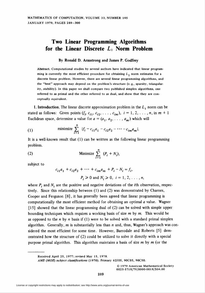
If we use the revised simplex approach to generate the tableau, then the basis
matrices will be of the form (after row interchanges)
"-C3-where (^ ) = C after row interchanges, B is an m by m matrix, R is an (« - m) by m
matrix, 0 is an m by (« - m) zero matrix, (CB) = f after row interchanges, and D is
an (n - m) by (n - m) matrix whose diagonal elements are either +1 or -1 and non-
diagonal elements are zeros. Due to the format of the basis matrix, the initial tableau
will also require the appropriate adjustments.
a
11
R
0
NB
I 0 -/
0/0
e e e
I 0 -/
0 / 0
eDRB~' - D
'B
¿r1
-DRB-
e e e
A",B
-B-1
DRB-
NB
-D
4
ÎR
0
ÍB
4
B~lfB
D(fR-RB~lfB)
e+eDRB~ eD eDRB' e + eD eD(fR -RB~lfB)
The marginal cost for (n - m) nonbasic N¡ (P¡) with the corresponding P. (N¡) in the
basis is 2. For the case where both N¡ and Pp m of each, are nonbasic, the marginal
cost for P¡ is 1 + eDRBk 1, and for N¡ it is 1 - eDRBk l, where Bk 1 is the kth
column of B~l, and c¡ = Bk = (cix, ci2, . . . , c¡n) is the kth row of B. At optimality,
the row of the marginal cost terms will be nonnegative, or this can be replaced by the
equivalent statement
(6) -KeDRBkl <l, k=l,2,...,m.
License or copyright restrictions may apply to redistribution; see http://www.ams.org/journal-terms-of-use
292 RONALD D. ARMSTRONG AND JAMES P. GODFREY
To assist in demonstrating the equivalence of the two algorithms under consider-
ation here, two index sets are defined as follows:
U = {i \P¡ is basic}, L = {i \N¡ is basic}.
Condition (6) can now be restated as
-1</2>|-E e,W!<1' k=l,2,...,m,\i&u íe¿ J
or defining
wk = (Z c¡- Z cSb^1, -l<wk<l, k= 1,2, ...,m.
Once it has been ascertained that the optimality conditions are not satisfied for
some /' (say / = /), then either Nt or P¡ is to enter the basis and the primal algorithm
proceeds to determine the LP variable to leave the basis. The standard procedure at
this stage is to take the minimum of the ratios
fk-CkB-% _
^kB~ql
(7)fk-CkB-lfi
pckB~' > 0, kEU, and
Bpc^-^0, kEL,
WkBo
where q is the row of B associated with the index / (c¡ = B ) and
(-1 if P¡ enters the basis,
P = \
1 1 if A, enters the basis.
The standard primal algorithm would now perform a pivot to remove the vector
chosen by the minimum ratio test from the basis and to enter either N¡ or P¡ into the
basis. However, the special purpose algorithms may perform several interchanges of
basis vectors before executing the pivot to bring either N¡ ox P¡ into the basis. Let t
be the value of k when the minimum ratio occurs in (7). Then the linear program-
ming variable to be removed from the basis will be either Nt or Pt, whichever is in the
basis. In order to clarify this process, suppose P¡ is to enter the basis, and Nt is to
leave the basis. If 1 + w + 2 \cfi~1 I > 0, then the standard pivoting procedure of
the simplex algorithm is carried out. If 1 + w + 2 \CfB~1 I < 0, then Pt will re-
place Nt in the basis, and the row of marginal costs are updated. This calculation is
achieved by adding twice the rth row of the current tableau to the row of the reduced
cost factors. The algorithm now returns to the minimum ratio test and finds the ratio
which is next to the smallest. The basic variable associated with this ratio is then
tested, as above, for removal by the standard pivoting technique or for interchange in
the basis with its corresponding dependent deviation variable. This procedure will
continue until P, is brought into the basis by the usual pivoting method, and then a new
vector will be sought to enter the basis by observing the values of the marginal cost
row, and the steps are repeated until optimality is reached.
License or copyright restrictions may apply to redistribution; see http://www.ams.org/journal-terms-of-use
ALGORITHMS FOR THE LINEAR DISCRETE Lj NORM PROBLEM 293
3. Development of Dual Algorithm (Abdelmalek). In this section, we shall
briefly develop the dual simplex method which Abdelmalek applies to LP (4). Re-
writing LP (4) in matrix notation and condensing the constant term in the objective
function, we obtain the following.
(8) Maximize fTb - fTe
subject to
CTb = CTe, 0<bt<2, i = 1, 2, . . . , n,
where bT = (bx, b2, . . . , bn) is the vector of the variables for this dual problem.
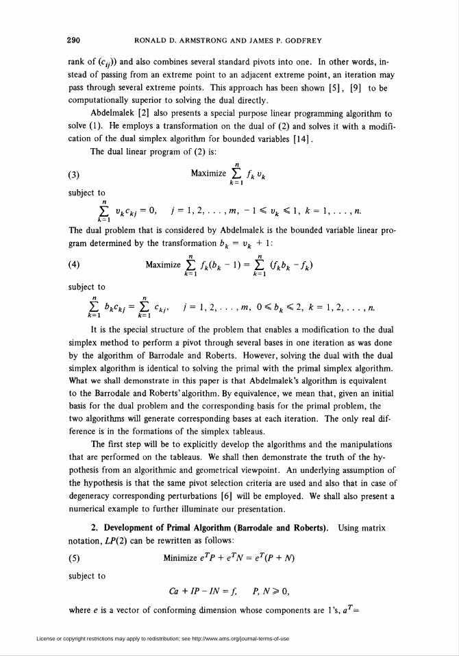
We shall now present the simplex tableau formulation that is employed by Abdel-
malek in solving LP (8). The notation is the same as in the preceding section.
[
BT on-
fl l.
B1 R1
-fTJB -fTJR
CTe
~eTf
iB-lfBy(B-1)
l\T
(B~ifBy i
B R1
-fT _fTJB JR
CTe
-eTf
I
0
(RB~l)T
fT(RB-l)T-fl
(CB-l)Te
(BL%fCT'e'-eTf
However, since some of the nonbasic elements associated with the columns of
(RB~l)T may be at their upper bound, we must modify the right-hand side to account
for this fact. Thus, the values of the kth basic variable bB,k) will be given by
**<*> = (BkV[cTe-2 J^j = (BkY [Be + Re - £ cl
=i+(V)rrz ci-zciL/ez, /er/ J
where U and L axe the index set of the nonbasic variables which are at their upper and
lower bound, respectively. (Further details on this can be found in Hadley [10].)
Nonbasic variables which are at their upper bound are recognized by the fact that the
associated entry in f^(RB~l)T -/J^will be negative. These variables will have anx
placed above their associated column in the tableau. Therefore, the tableau may have
the following form:
/ (RB~l)T
cT(Db-UT _ fT f!ibB0 f¿(RB-y-fT
At this point a brief description of the steps from Abdelmalek's algorithm is
0 + 1 ff-I.frjeu jGL
given.
1. Select a variable to become primal feasible (vector to leave the basis) by the
rule
License or copyright restrictions may apply to redistribution; see http://www.ams.org/journal-terms-of-use
294 RONALD D. ARMSTRONG AND JAMES P. GODFREY
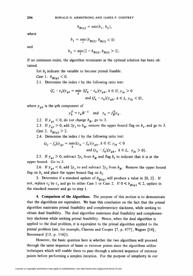
bB(q) =iran{*i. b2},
where
bx =mm{bB(i),bBt¡)<0}
andb2 = min{2 - bB(i), bB>i) > 2}.
If no minimum exists, the algorithm terminates as the optimal solution has been ob-
tained.
Let b¡ indicate the variable to become primal feasible.
Case 1. bB, <. < 0.
2.1. Determine the index t by the following ratio test:
(ft - zt)lyqt = mül Ofk - zk)lyqk> kEU, yik > 0
and (fk - zk)/yqk, k E L, yik < 0},
where y k is the ¿7th component of
yl = ckB~l and zk=fSyk-
2.2. If y t < 0, do not change bB , go to 3.
2.3. If y t > 0, add 2yt to bB, remove the upper bound flag on bt, and go to 3.
Case 2. bB(q) > 2.
2.4. Determine the index t by the following ratio test:
(zt-ft)lyqt = min{(zk -fk)lyqk, kEU, yik < 0
and (zk ~fk)/yqk, k E L, yik > 0}.
2.5. lfyqr > 0, subtract 2y, from bB and flag b, to indicate that it is at the
upper bound. Go to 3.
2.6. If y t < 0, add 2yt to and subtract 2y¡ from bB. Remove the upper bound
flag on bt and place the upper bound flag on b¡.
3. Determine if a standard update of bB, -, will produce a value in [0, 2]. If
not, replace c¡ by ct and go to either Case 1 or Case 2. If 0 < bB, % < 2, update in
the standard manner and go to step 1.
4. Comparison of the Algorithms. The purpose of this section is to demonstrate
that the algorithms are equivalent. We base this conclusion on the fact that the primal
algorithm maintains primal feasibility and complementary slackness, while seeking to
obtain dual feasibility. The dual algorithm maintains dual feasibility and complemen-
tary slackness while seeking primal feasibility. Hence, when the dual algorithm is
applied to the dual problem, it is equivalent to the primal algorithm applied to the
primal problem (see, for example, Chames and Cooper [7, p. 477], Wagner [14],
Simonnard [13, p. 116]).
However, the basic question here is whether the two algorithms will proceed
through the same sequence of bases or extreme points since the algorithms utilize
techniques which will enable them to pass through a selected sequence of extreme
points before performing a simplex iteration. For the purpose of simplicity in our
License or copyright restrictions may apply to redistribution; see http://www.ams.org/journal-terms-of-use
ALGORITHMS FOR THE LINEAR DISCRETE Lx NORM PROBLEM 295
development, we shall assume that degeneracy is not present in our problem.
In general, we shall illustrate how the steps performed on the dual relate to the
primal. A negative zk —fk in the dual and flagging the kth column (bk = 2) corre-
sponds to having a Pk in the basis of the primal. Also, when bk is nonbasic with
bk = 0 in the dual problem, Nk is in the basis of the primal. If bk is basic in the dual,
then Nk and Pk are nonbasic in the primal. The fk - zks in the dual are the same as
the deviations in the primal. Therefore, the ranking of the minimum ratios will be in
the same sequence for each of the algorithms so that corresponding vectors will enter
and leave the basis during a pivot. This can be observed directly by noting that the
same vector (assuming no ties exist in the ratios) must enter the basis in both algo-
rithms, because there is a unique vector whose entry into basis will maintain the dual
feasibility of (8) and force primal feasibility in the pivot row. Both the rules given by
Abdelmalek and Barrodale and Roberts do this although they are stated in slightly
different forms.
The primal algorithm attempts to place the dual variables in the interval [-1, 1 ].
The dual algorithm works towards placing the primal variables of the dual (which are
the dual variables of the primal) in the interval [0, 2]. The difference in the intervals
has been brought about by the transformation employed by Abdelmalek. Thus, there
will be a difference between these variables which is created by the transformation.
In addition, the differences in tableaus in terms of the signs of the elements can be
accounted for by the utilization of the D matrix in the primal. This matrix is not
employed by Abdelmalek in the dual, but he utilizes the x above the columns to flag
the variables at their upper bounds.
Additional aspects such as the value of the objective function being the same at
each extreme point of the sequence is clearly observable from the tableaus which were
developed. The process of adding (or subtracting) the term 2yt is the same in the al-
gorithms.
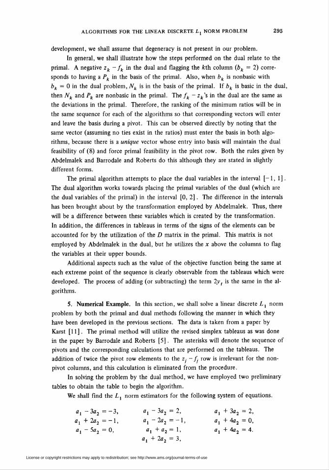
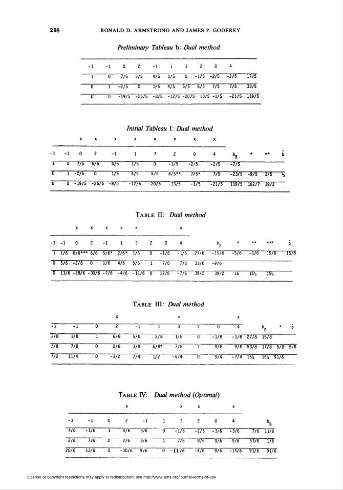
5. Numerical Example. In this section, we shall solve a linear discrete Lx norm
problem by both the primal and dual methods following the manner in which they
have been developed in the previous sections. The data is taken from a paper by
Karst [11]. The primal method will utilize the revised simplex tableaus as was done
in the paper by Barrodale and Roberts [5]. The asterisks will denote the sequence of
pivots and the corresponding calculations that are performed on the tableaus. The
addition of twice the pivot row elements to the z;- - / row is irrelevant for the non-
pivot columns, and this calculation is eliminated from the procedure.
In solving the problem by the dual method, we have employed two preliminary
tables to obtain the table to begin the algorithm.
We shall find the Lx norm estimators for the following system of equations.
ax - 3a2 = -3, a^~ 3a2 = 2, ax + 3a2 = 2,
ax+2a2=-l, ax-2a2=-l, ax+4a2=0,
ax - 5a2 = 0, ax + a2 = 1, ax + 4a2 = 4.
ax + 2a2 = 3,
License or copyright restrictions may apply to redistribution; see http://www.ams.org/journal-terms-of-use
296 RONALD D. ARMSTRONG AND JAMES P. GODFREY
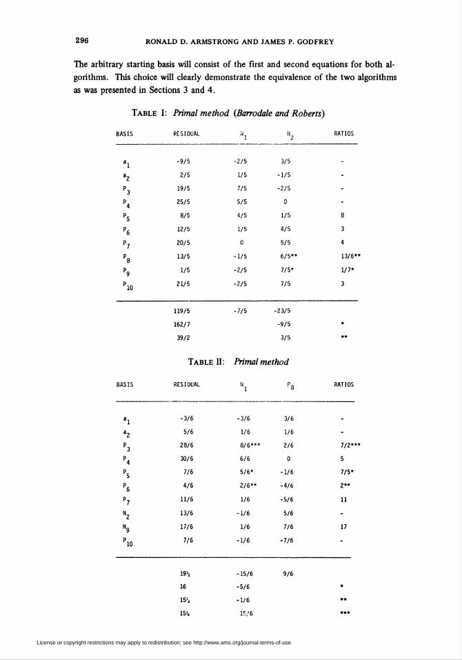
The arbitrary starting basis will consist of the first and second equations for both al-
gorithms. This choice will clearly demonstrate the equivalence of the two algorithms
as was presented in Sections 3 and 4.
Table I: Primal method (Barrodale and Roberts)
BASIS RESIDUAL H N RATIOS
a -9/5 -2/5 3/5
a2 2/5 1/5 -1/5
P3 19/5 7/5 -2/5
P. 25/5 5/5 04
P5 8/5 4/5 1/5 8
P6 12/5 1/5 4/5 3
P? 20/5 0 5/5 4
P0 13/5 -1/5 6/5** 13/6*
P9 1/5 -2/5 7/5* 1/7*
P10 21/5 -2/5 7/5 3
119/5 -7/5 -23/5
162/7 -9/5
39/2 3/5
Table II: Primal method
BASIS RESIDUAL M P„ RATIOS1 u
ix -3/6 -3/6 3/6
a2 5/6 1/6 1/6
P3 28/6 8/6*** 2/6 7/2***
P, 30/6 6/6 0 54
P5 7/6 5/6* -1/6 7/5*
P6 4/6 2/6** -4/b 2**
P7 11/6 1/6 -5/6 11
N2 13/6 -1/6 5/6
Ng 17/6 1/6 7/6 17
P10 7/6 -1/6 -7/6
19!j -15/6 9/6
16 -5/6
15'a -1/6
151, 15/6
License or copyright restrictions may apply to redistribution; see http://www.ams.org/journal-terms-of-use
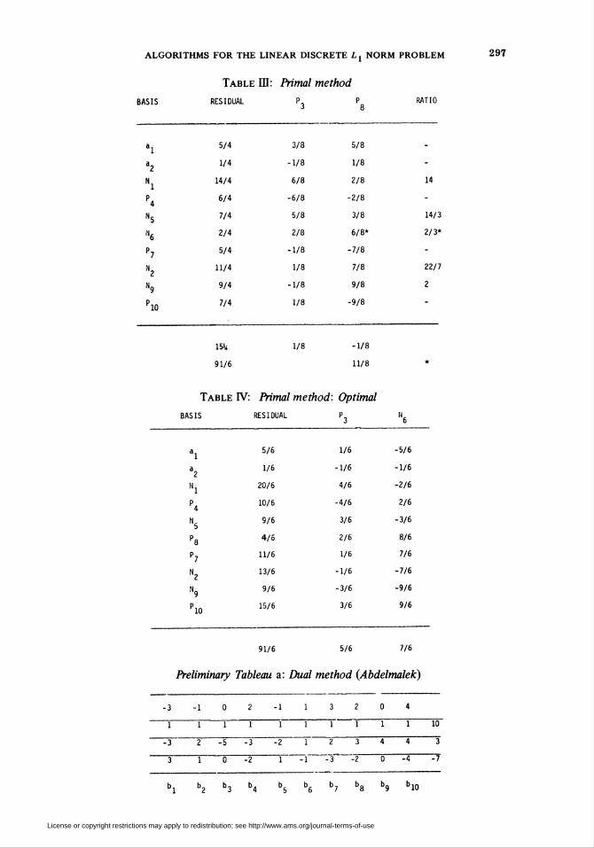
ALGORITHMS FOR THE LINEAR DISCRETE Lx NORM PROBLEM 297
Table HI: Primal method
BASIS RESIDUAL P, P RATIO3 8
aj 5/4 3/8 5/8
a2 1/4 -1/8 1/8
N 14/4 6/8 2/8 14
P. 6/4 -6/8 -2/84
N5 7/4 5/8 3/8 14/3
fig 2/4 2/8 6/8* 2/3*
P? 5/4 -1/8 -7/8
H 11/4 1/8 7/8 22/7
Ng 9/4 -1/8 9/8 2
P10 7/4 1/8 -9/8
15% 1/8 -1/8
91/6 11/8
Table IV: Primal method: Optimal
BASIS RESIDUAL P, M,3 6
a 5/6 1/6 -5/6
21/6 -1/6 -1/6
Nj 20/6 4/6 -2/6
P. 10/6 -4/6 2/64
N 9/6 3/6 -3/6
P8 4/6 2/6 8/6
P? 11/6 1/6 7/6
N2 13/6 -1/6 -7/6
Ng 9/6 -3/6 -9/6
P1Q 15/6 3/6 9/6
91/6 5/6 7/6
Preliminary Tableau a: Dual method (Abdelmalek)
-10 2-113204
i i i i Ï P "T i Î~2 3) ^3 "-Í i 2 3 4 4
10
-7
bl b2 b3 b4 b5 b6 b7 b8 b9 b10
License or copyright restrictions may apply to redistribution; see http://www.ams.org/journal-terms-of-use
298 RONALD D. ARMSTRONG AND JAMES P. GODFREY
Preliminary Tableau b: Dual method
-3-102-113204
~i B 775 575 475 T/5 0 -1/5 -2/1 =775 Î775
"5 1 -275 B Í75 475 "575 675 775 7/5 3375
~3 0 =T9/b -25/5 -8/5 -1275 -20/5 13/5 -1/5 -21/5 119/5
Initial Tableau I : Dual method
xxxxxxxx
-3-10 2-1 1 3 2 0 4 b„ * ** b
1 B 775 575 4/5 175 B ~ï/5~ ~275 "^275 ^775
"Ö 1 -2/5 S 175 T75 5/5 6/5** TTF* 775 -23/5 -9/5 375 Ç
"5 0 -19/5 -25/5 -8/5 -12/5 ^2075 "lTTS -T/5 ^2175 119/5 162/7 39/2
Table II: Dual method
X X X X X X
-3-102-113204 b3 ****** £
T 1/6 8/6*** 6/6 5/6* 2/6* 1/6 B ^T/l ~l7"6 2776 -15/6 ^TT6 rT/6 1575 1575
0 5/6 -2/6 (5 176 471 576 Î 776 776 3376 ^¡78
0 13/6 -28/6 -30/6 -7/6 -4/6 -fi/TT) 1775 "776 3972 3972 Î6 Ï5Ç 155
Table III: Dual method
XXX
^3 ~\ B 2 ~1 Ï 3 2 ~ "B 4~ bn * bB
Ö71 178 î 678 5/8 278 178 B "HTS -1/8 27/8 15/8
173 778 B 278 378 578* 778 I 978 9/8 53/8 17/8 5/8 5/6
772 ÏÏ74 B ^3?2 774 Î72 -5/4 15 974 -7/4 15% 15!. 91/6
Table IV: Dual method (Optimal)
X XXX
-3-102-113204 b
"475 ^176 i 476 375 o -"l/l -276 "371 ^376 7/1 TiTl
2/6 776 B 276 371 Ï 771 876" 976 976 5376 Í/1
2Ô76 13/6 0 -Wß "9/6 Ö" ~^TÏ '/l ^4/1 9/1 "ll/l 9Î76 9Ï71
License or copyright restrictions may apply to redistribution; see http://www.ams.org/journal-terms-of-use
ALGORITHMS FOR THE LINEAR DISCRETE Lx NORM PROBLEM 299
6. Conclusions. Because Abdelmalek's algorithm is essentially equivalent to the
Barrodale and Roberts' algorithm, Abdelmalek's comment that the methods are com-
parable in terms of both speed and number of iterations is not surprising. A set of
comprehensive tests performed by the National Bureau of Standards [9] on four Lx
norm codes clearly demonstrates this fact. The only differences between the two algo-
rithms involve the choice of an initial basis and the heuristic rules for breaking ties. Of
course, there are an infinite number of ways any linear programming "algorithm" can
be implemented-e.g., full tableau, revised simplex with product form or explicit in-
verse, multiple pricing, etc. The unique thing about the Barrodale and Roberts' algo-
rithm is the ability to combine several standard iterations into one.
It does appear that the simplex algorithm of linear programming is the most effi-
cient method to solve the linear discrete Lx norm problem. A superior nonsimplex
based algorithm would amount to finding a better way to solve a linear programming
problem. This topic has been studied for many years, and the iterative technique of
passing from extreme point to extreme point common to virtually all linear program-
ming codes remains the most efficient.
Current research on solving the linear discrete Lx norm problem seems to involve
extensions of the Barrodale and Roberts' algorithm. McCormick and Sposito [12] dem-
onstrate how the L2 norm estimate can be utilized to accelerate the convergence of the
Barrodale and Roberts' algorithm. Armstrong and Hultz [4] extend the algorithm to
handle additional linear constraints on the parameters. Finally, Armstrong and Frome
[3] demonstrate how a network structure can be utilized when obtaining Lx norm
estimates for two-way tables.
Department of General Business
Graduate School of Business
The University of Texas
Austin, Texas 78712
Economic Planning Division
Central Intelligence Agency
Washington, D. C. 22101
1. N. N. ABDELMALEK, "On the discrete linear Lx approximation and Lx solutions of
overdetermined linear equations,"/. Approximation Theory, v. 11, 1974, pp. 38—53.
2. N. N. ABDELMALEK, "An efficient method for the discrete linear Lx approximation
problem," Math. Comp., v. 29, 1975, pp. 844-850.
3. R. D. ARMSTRONG & E. L. FROME, "Least absolute value estimators for one-way
and two-way tables," Naval Res. Logist. Quart. (To appear.)
4. R. D. ARMSTRONG & J. W. HULTZ, "An algorithm for a restricted discrete approxi-
mation problem in the Lx norm," SIAM J. Numer. Anal., v. 14, 1977, pp. 555-565.
5. I. BARRODALE & F. D. K. ROBERTS, "An improved algorithm for discrete Lx linear
approximation," SIAM J. Numer. Anal., v. 10, 1973, pp. 839-848.
6. A. CHARNES, "Optimality and degeneracy in linear programming," Econometrica, v. 20
(2), 1952, pp. 160-170.7. A. CHARNES & W. W. COOPER, Management Models and Industrial Applications of
Linear Programming, Vol. II, Wiley, New York, 1961.8. A. CHARNES, W. W. COOPER & R. FERGUSON, "Optimal estimation of executive
compensation by linear programming," Management Sei., v. 2, 1955, pp. 138—151.
9. J. GILSINN, K. HOFFMAN, R. H. F. JACKSON, E. LEYENDECKER, P. SAUNDERS &
D. SHIER, "Methodology and analysis for comparing discrete linear Lx approximation codes,"
Comm. Statist., v. B6(4), 1977.
License or copyright restrictions may apply to redistribution; see http://www.ams.org/journal-terms-of-use
300 RONALD D. ARMSTRONG AND JAMES P. GODFREY
10. G. HADLEY, Linear Programming, Addison-Wesley, Reading, Mass., 1962.
11. O. J. KARST, "Linear curve fitting using least deviations," /. Amer. Statist. Assoc, v.
53, 1958, pp. 118-132.
12. G. F. McCORMICK & V. A. SPOSITO, "Using the Lj-estimator in the ¿j-estimation,"
SIAM J. Numer. Anal, v. 13, 1976, pp. 337-343.
13. M. SIMONNARD, Linear Programming, Prentice-Hall, Englewood Cliffs, N.J., 1966.
14. H. M. WAGNER, "The dual simplex algorithm for bounded variables," Naval Res.
Logist Quart, v. 5, 1958, pp. 257-261.
15. H. M. WAGNER, "Linear programming techniques for regression analysis," /. Amer.
Statist. Assoc, v. 54, 1959, pp. 206-212.
License or copyright restrictions may apply to redistribution; see http://www.ams.org/journal-terms-of-use


![Ppt0000011.ppt [Lecture seule]...Message-passing on chains Global minimum in linear time Optimization proceeds in two passes: Forward pass (dynamic programming) Backward pass prq s](https://static.documents.pub/doc/80x56/5ff8631a599c3e071c6bba30/lecture-seule-message-passing-on-chains-global-minimum-in-linear-time-optimization.jpg)


