arX

iv:0

708.

1780

v2 [

nucl

-th]

18

Dec

200

7

Two-particle scattering on the lattice:

Phase shifts, spin-orbit coupling, and mixing angles

Bugra Borasoya, Evgeny Epelbauma,b, Hermann Krebsa,b, Dean Leec,a, Ulf-G. Meißnera,b

aHelmholtz-Institut fur Strahlen- und Kernphysik (Theorie) Universitat Bonn,

Nußallee 14-16, D-53115 Bonn, Germany

bInstitut fur Kernphysik (Theorie), Forschungszentrum Julich, D-52425 Julich, Germany

cDepartment of Physics, North Carolina State University, Raleigh, NC 27695, USA

Abstract

We determine two-particle scattering phase shifts and mixing angles for quantum theories

defined with lattice regularization. The method is suitable for any nonrelativistic effective

theory of point particles on the lattice. In the center-of-mass frame of the two-particle

system we impose a hard spherical wall at some fixed large radius. For channels without

partial-wave mixing the partial-wave phase shifts are determined from the energies of the

nearly-spherical standing waves. For channels with partial-wave mixing further information

is extracted by decomposing the standing wave at the wall boundary into spherical harmon-

ics, and we solve coupled-channels equations to extract the phase shifts and mixing angles.

The method is illustrated and tested by computing phase shifts and mixing angles on the

lattice for spin-1/2 particles with an attractive Gaussian potential containing both central

and tensor force parts.

1

I. INTRODUCTION

There have been several recent studies on the subject of lattice simulations for low-energy

nuclear physics using effective interactions [1, 2, 3, 4, 5, 6, 7, 8, 9, 10, 11, 12, 13, 14]. Similar

lattice effective field theory techniques have been used to study cold atomic Fermi systems

in the limit of short-range interactions and large scattering length [15, 16, 17, 18, 19, 20, 21].

In nearly all cases the connection between lattice interactions and physical observables is

made using some variant of Luscher’s result [22, 23, 24] relating the energy levels of two-

body states in a finite-volume cubic box with periodic boundaries to the infinite-volume

scattering matrix.

Luscher’s method has been extended in a number of different ways. Several studies

have looked at asymmetric boxes [25, 26], while another considered small volumes where

the lattice length L is smaller than the scattering length [27]. There have also been studies

of moving frames [28, 29], winding of the interaction around the periodic boundary [30],

modifications at finite lattice spacing [8], and techniques to distinguish shallow bound states

from scattering states using Levinson’s theorem [31]. A very recent study derived finite

volume formulas for systems of n bosons with short-range repulsive interactions [32].

While Luscher’s method has been very useful at low momenta, there is currently no

technique which is able to determine phase shifts on the lattice at higher energies and higher

orbital angular momenta. There is also no technique which can accurately measure spin-

orbit coupling and partial-wave mixing on the lattice. The physics of spin-orbit coupling and

partial-wave mixing is difficult to extract using Luscher’s method due to artifacts generated

by the periodic cubic boundary. An example of this problem is shown in the summary

and discussion section of this paper. Any method overcoming these theoretical problems

would probably not be numerically practical when applied to lattice simulations of quantum

chromodynamics. This is because each individual hadron must be constructed as a bound

state of quark and gluon fields, and the Monte Carlo signal for hadron-hadron scattering

states well above threshold would be very weak. However for an effective lattice theory

of fundamental point particles, such a technique should be numerically viable since the full

two-particle spectrum is relatively easy to compute.

In this paper we discuss a simple method which directly measures two-particle phase shifts

and mixing angles on the lattice. In the center-of-mass frame of the two-particle system

2

we impose a hard spherical wall boundary condition at some large radius. Phase shifts

and mixing angles are determined from properties of the nearly-spherical standing waves

produced by the wall boundary. The method is suitable for any nonrelativistic effective

theory of point particles on the lattice with or without spin. We test the method on the

lattice using an attractive Gaussian potential for spin-1/2 particles containing both central

and tensor force parts.

The organization of the paper is as follows. We first discuss representations of the cubic

rotational group. We then introduce the test potential and solve the S = 0 channels and

uncoupled S = 1 channels up to J = 4 using the spherical wall method. We then discuss

coupled partial waves with a common nodal constraint and the coupled equations needed to

solve for the L = J −1 and J +1 phase shifts and mixing angle for total angular momentum

J . Finally we solve the coupled S = 1 channels on the lattice up to J = 4 and discuss

applications of the technique.

II. CUBIC ROTATIONAL GROUP

Our choice of lattice regularization reduces the SO(3) rotational symmetry of continuous

space to the cubic rotational group SO(3, Z). This consists of 24 group elements generated

by products of π/2 rotations about the x, y, z axes. Since SO(3, Z) is discrete, we cannot

define angular momentum operators Jx, Jy, Jz in the usual sense. However if Rz (π/2) is

the group element for a π/2 rotation about the z axis, we can use the SO(3) relation

Rz (π/2) = exp[

−iπ

2Jz

]

(1)

to define Jz. The eigenvalues of Jz are integers modulo 4. Jx and Jy can be defined in the

same manner.

There are five irreducible representations of the cubic rotational group. These are usually

written as A1, T1, E, T2, and A2. Some of their properties and examples in terms of spherical

harmonics YL,Lz(θ, φ) are listed in Table I.

The 2J + 1 elements of the total angular momentum J representation of SO(3) break up

into smaller pieces consisting of the five irreducible representations. Examples for J ≤ 7

are shown in Table II [33].

In this analysis we consider the scattering of two identical particles and assume that

3

TABLE I: Irreducible SO(3, Z) representations

Representation Jz Example

A1 0mod 4 Y0,0

T1 0, 1, 3mod 4 {Y1,0, Y1,1, Y1,−1}

E 0, 2mod 4{

Y2,0,Y2,−2+Y2,2√

2

}

T2 1, 2, 3mod 4{

Y2,1,Y2,−2−Y2,2√

2, Y2,−1

}

A2 2mod 4Y3,2−Y3,−2√

2

TABLE II: SO(3, Z) decompositions for J ≤ 7

SO(3) SO(3, Z)

J = 0 A1

J = 1 T1

J = 2 E ⊕ T2

J = 3 T1 ⊕ T2 ⊕ A2

J = 4 A1 ⊕ T1 ⊕ E ⊕ T2

J = 5 T1 ⊕ T1 ⊕ E ⊕ T2

J = 6 A1 ⊕ T1 ⊕ E ⊕ T2 ⊕ T2 ⊕ A2

J = 7 T1 ⊕ T1 ⊕ E ⊕ T2 ⊕ T2 ⊕ A2

the interactions are parity conserving. Therefore in continuous space the two particles

share the same group representation for intrinsic spin and the same group representation

for all other internal quantum symmetries. As a result each two-particle state must be

symmetric or antisymmetric under parity and symmetric or antisymmetric with respect

to internal symmetry quantum numbers. Once these are fixed the overall Fermi or Bose

statistics determines whether the total intrinsic spin combination must be symmetric or

antisymmetric.

There are well-known problems associated with massless fermions on the lattice. How-

ever for nonrelativistic particles one can easily find a lattice Hamiltonian or Euclidean action

which maintains exact parity invariance and all internal symmetries. Therefore the sym-

metry or antisymmetry of intrinsic spin on the lattice is unambiguous and the same as in

continuous space. For two spin-1/2 particles where the total intrinsic spin is S = 0 or

4

S = 1, this is enough to specify the intrinsic spin representation completely. If the intrinsic

spin is symmetric then the SO(3, Z) representation is A1. If the intrinsic spin is antisym-

metric then the SO(3, Z) representation is T1. These are in one-to-one correspondence with

the representations S = 0 and S = 1 in continuous space, respectively, and so there is no

confusion in borrowing the continuous space names for the two cases. For particles with

higher intrinsic spin, there is in general some unphysical mixing on the lattice among even

values of S and among odd values of S. The same mixing on the lattice occurs among even

values and odd values of orbital angular momentum L regardless of the intrinsic spin.

III. TEST POTENTIAL

There is an endless variety of different interactions one can study on the lattice. For our

analysis we choose a simple pedagogical example for which the continuum limit is relatively

easy to compute. We choose a bounded short-range potential producing both a central

force and tensor force. This yields all of the essential complications of spin-orbit coupling

with partial-wave mixing while leaving out additional issues of ultraviolet divergences and

singular interactions. We take a system of identical spin-1/2 particles with mass m and a

spin-dependent potential,

V (~r ) = C

{

1 +r2

R20

[3 (r · ~σ1) (r · ~σ2) − ~σ1 · ~σ2]

}

exp

(

−1

2

r2

R20

)

. (2)

The range of the potential is set by the parameter R0. We leave the internal symmetry

group unspecified and consider all possible combinations of symmetry or antisymmetry for

parity and intrinsic spin.

The tensor operator

S12(r) = 3 (r · ~σ1) (r · ~σ2) − ~σ1 · ~σ2 (3)

is of considerable general interest in physics. It is produced both by one-pion exchange in

low-energy nuclear physics as well as by magnetic and electric dipole interactions in atoms

and molecules. The parameters C, R0, and m we choose are motivated by low-energy

5

nuclear physics,

C = −2 MeV, (4)

R0 = 2 × 10−2 MeV−1, (5)

m = 938.92 MeV. (6)

This produces a very shallow bound state in the 3S(D)1 channel with energy −0.155 MeV.

The parenthesis in our spectroscopic notation indicates a mixture of two partial waves. For

example 3S(D)1 indicates a mixture of S and D partial waves. The ordering of the partial

waves, S(D) rather than D(S), indicates that this state becomes a pure S wave when the

tensor part of the interaction is continuously dialed down to zero. This identification is

unambiguous in finite volume systems where the energy levels are discrete.

For total intrinsic spin S = 0 the tensor operator S12 vanishes. And so for this case it

suffices to consider just the central part of the potential,

V0(~r ) = C exp

(

−1

2

r2

R20

)

, (7)

for particles with no intrinsic spin at all. We start first with this simplest case. Afterwards

we consider S = 1 for uncoupled channels and then finally S = 1 in coupled channels.

IV. INTRINSIC SPIN S = 0

We measure phase shifts by imposing a hard spherical wall boundary on the relative

separation between the two particles at some chosen radius Rwall. Viewed in the center-of-

mass frame we solve the Schrodinger equation for spherical standing waves which vanish at

r = Rwall. This is sketched in Fig. 1. We are of course assuming that the original lattice

system is large enough to hold a sphere of radius Rwall. The reason for this spherical wall

is to remove copies of the two-particle interactions due to the periodic boundaries of the

lattice. It is this feature that distinguishes our method from Luscher’s method [24].

For values of r beyond the range of the interaction, the spherical standing wave in con-

tinuous space can be decomposed as a superposition of products of spherical harmonics and

spherical Bessel functions,

[cos δL × jL(kr) − sin δL × yL(kr)] YL,Lz(θ, φ), (8)

6

Rwall

FIG. 1: Spherical wall imposed in the center-of-mass frame.

where the center-of-mass energy of the spherical wave is

E = 2 ×k2

2m=

k2

m, (9)

and the phase shift for partial wave L is δL. Therefore we know k from the energy E, and

the phase shift δL is determined by setting the wavefunction (8) equal to zero at the wall

boundary,

cos δL × jL(kRwall) = sin δL × yL(kRwall), (10)

δL = tan−1

[

jL(kRwall)

yL(kRwall)

]

. (11)

On the lattice there is some ambiguity on the precise value of Rwall since the components

of ~r must be integer multiples of the lattice spacing. We resolve this ambiguity by fine-

tuning the value of Rwall for each standing wave so that δL equals zero when the particles

are non-interacting. This is illustrated in the following discussion of the lattice calculation.

V. LATTICE CALCULATION FOR S = 0

Since our method is intended as a tool for simulations of few- and many-body systems

using lattice effective field theory, we present the analysis using the standard formalism of

lattice field theory developed in the literature. For the free part of the lattice action we

use the same lattice action defined in [13] with spatial lattice spacing a = (100 MeV)−1

and temporal lattice spacing at = (70 MeV)−1. We define αt as the ratio between lattice

spacings, αt = at/a. Throughout we use dimensionless parameters and operators, which

7

correspond with physical values multiplied by the appropriate power of a. Final results are

presented in physical units with the corresponding unit stated explicitly.

Since the temporal lattice spacing is nonzero we work with transfer matrices rather than

the Hamiltonian directly. In simple terms the transfer matrix is just the exponential of the

Hamiltonian exp(−H∆t), where ∆t equals one temporal lattice spacing. More precisely

the free-particle transfer matrix is defined as

Mfree ≡ : exp (−Hfreeαt) : , (12)

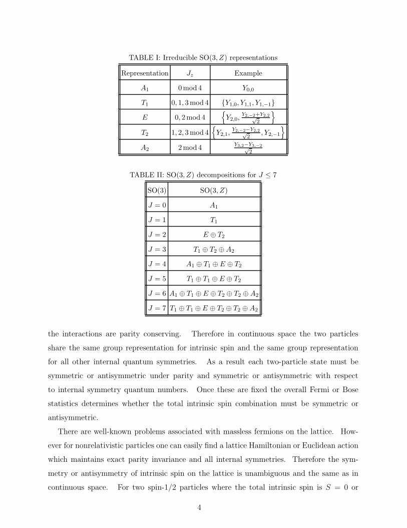
where the :: symbols indicate normal ordering. We use the O(a4)-improved free lattice

Hamiltonian,

Hfree =49

12m

∑

~n

∑

j=↑,↓

a†j(~n)aj(~n)

−3

4m

∑

~n

∑

j=↑,↓

∑

l=1,2,3

[

a†j(~n)aj(~n + l) + a†

j(~n)aj(~n − l)]

+3

40m

∑

~n

∑

j=↑,↓

∑

l=1,2,3

[

a†j(~n)aj(~n + 2l) + a†

j(~n)aj(~n − 2l)]

−1

180m

∑

~n

∑

j=↑,↓

∑

l=1,2,3

[

a†j(~n)aj(~n + 3l) + a†

j(~n)aj(~n − 3l)]

. (13)

The vector ~n denotes integer-valued coordinate vectors on a spatial three-dimensional lattice,

and l = 1, 2, 3 are lattice unit vectors in each of the spatial directions.

Since the potential energy is finite we can take the lattice potential at ~n to agree with

the continuum potential at ~r = ~na. For S = 0 we can omit the tensor part of the potential,

and so the transfer matrix is

M ≡ : exp

−Hfreeαt −αt

2

∑

~n1,~n2

V0(~n1 − ~n2)ρa†,a(~n1)ρ

a†,a(~n2)

: , (14)

where ρa†,a(~n) is the particle density operator

ρa†,a(~n) =∑

j=↑,↓

a†j(~n)aj(~n). (15)

We calculate eigenvalues of the transfer matrix using the Lanczos method [34]. In the

transfer matrix formalism eigenvalues of the transfer matrix are interpreted as exponentials

of the energy,

M |Ψ〉 = λ |Ψ〉 = e−Eαt |Ψ〉 . (16)

8

0

2

4

6

8

10

12

0 1 2 3

E (

MeV

)

Lz mod 4

even parity

1S

1D

2S

1G

2D

3S

1I

A1T1E T2A2

0

2

4

6

8

10

12

0 1 2 3

E (

MeV

)Lz mod 4

odd parity

1P

1F

2P

1H

2F

3P

0

2

4

6

8

10

12

0 1 2 3

E (

MeV

)Lz mod 4

odd parity

1P

1F

2P

1H

2F

3P

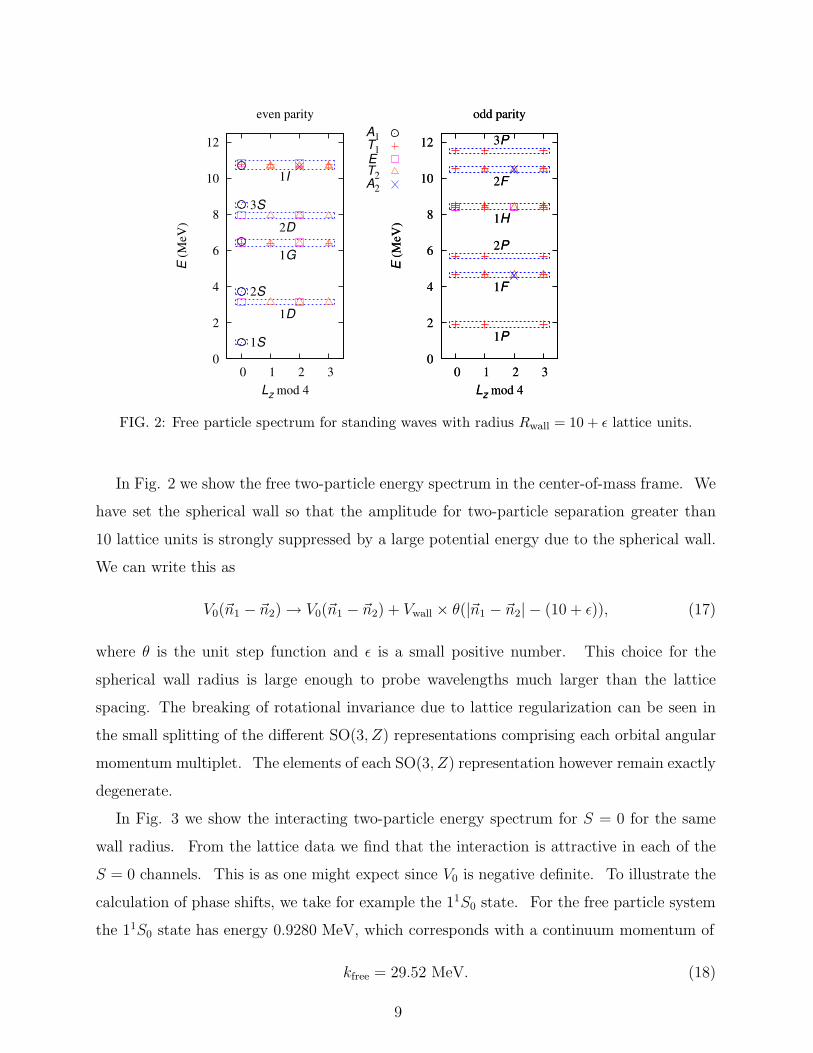
FIG. 2: Free particle spectrum for standing waves with radius Rwall = 10 + ǫ lattice units.

In Fig. 2 we show the free two-particle energy spectrum in the center-of-mass frame. We

have set the spherical wall so that the amplitude for two-particle separation greater than

10 lattice units is strongly suppressed by a large potential energy due to the spherical wall.

We can write this as

V0(~n1 − ~n2) → V0(~n1 − ~n2) + Vwall × θ(|~n1 − ~n2| − (10 + ǫ)), (17)

where θ is the unit step function and ǫ is a small positive number. This choice for the

spherical wall radius is large enough to probe wavelengths much larger than the lattice

spacing. The breaking of rotational invariance due to lattice regularization can be seen in

the small splitting of the different SO(3, Z) representations comprising each orbital angular

momentum multiplet. The elements of each SO(3, Z) representation however remain exactly

degenerate.

In Fig. 3 we show the interacting two-particle energy spectrum for S = 0 for the same

wall radius. From the lattice data we find that the interaction is attractive in each of the

S = 0 channels. This is as one might expect since V0 is negative definite. To illustrate the

calculation of phase shifts, we take for example the 11S0 state. For the free particle system

the 11S0 state has energy 0.9280 MeV, which corresponds with a continuum momentum of

kfree = 29.52 MeV. (18)

9

0

1

2

3

4

5

6

0 1 2 3

E (

MeV

)

Lz mod 4

S = 0, even parity

11S0

21S0

11D2

11G4

A1T1E T2A2

0

1

2

3

4

5

6

0 1 2 3

E (

MeV

)

Lz mod 4

S = 0, odd parity

11P1

11F3

21P1

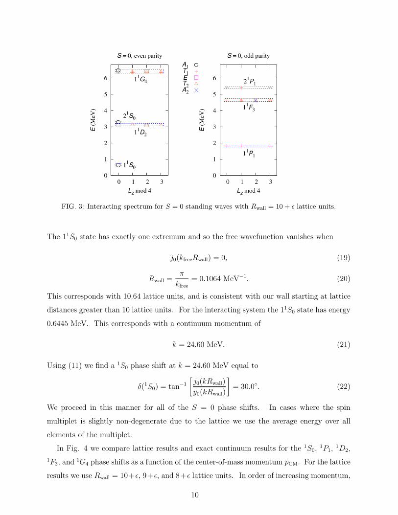
FIG. 3: Interacting spectrum for S = 0 standing waves with Rwall = 10 + ǫ lattice units.

The 11S0 state has exactly one extremum and so the free wavefunction vanishes when

j0(kfreeRwall) = 0, (19)

Rwall =π

kfree= 0.1064 MeV−1. (20)

This corresponds with 10.64 lattice units, and is consistent with our wall starting at lattice

distances greater than 10 lattice units. For the interacting system the 11S0 state has energy

0.6445 MeV. This corresponds with a continuum momentum of

k = 24.60 MeV. (21)

Using (11) we find a 1S0 phase shift at k = 24.60 MeV equal to

δ(1S0) = tan−1

[

j0(kRwall)

y0(kRwall)

]

= 30.0◦. (22)

We proceed in this manner for all of the S = 0 phase shifts. In cases where the spin

multiplet is slightly non-degenerate due to the lattice we use the average energy over all

elements of the multiplet.

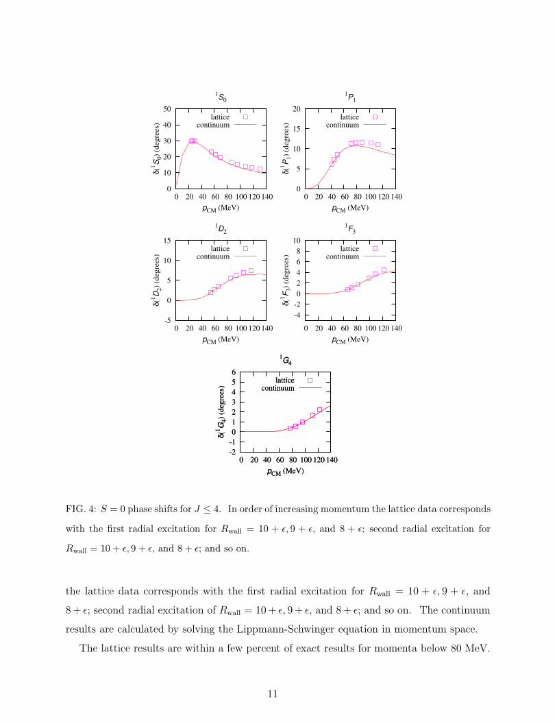
In Fig. 4 we compare lattice results and exact continuum results for the 1S0,1P1,

1D2,

1F3, and 1G4 phase shifts as a function of the center-of-mass momentum pCM. For the lattice

results we use Rwall = 10+ǫ, 9+ǫ, and 8+ǫ lattice units. In order of increasing momentum,

10

0

10

20

30

40

50

0 20 40 60 80 100 120 140

pCM (MeV)

1S0

δ(1S

0)

(deg

rees

)

latticecontinuum

0

5

10

15

20

0 20 40 60 80 100 120 140

pCM (MeV)

1P1

δ(1P

1)

(deg

rees

)

latticecontinuum

-5

0

5

10

15

0 20 40 60 80 100 120 140

pCM (MeV)

1D2

δ(1D

2)

(deg

rees

)

latticecontinuum

-4

-2

0

2

4

6

8

10

0 20 40 60 80 100 120 140

pCM (MeV)

1F3

δ(1F

3)

(deg

rees

)

latticecontinuum

-2

-1

0

1

2

3

4

5

6

0 20 40 60 80 100 120 140

pCM (MeV)

1G4

δ(1G

4)

(deg

rees

)

latticecontinuum

-2

-1

0

1

2

3

4

5

6

0 20 40 60 80 100 120 140

pCM (MeV)

1G4

δ(1G

4)

(deg

rees

)

latticecontinuum

FIG. 4: S = 0 phase shifts for J ≤ 4. In order of increasing momentum the lattice data corresponds

with the first radial excitation for Rwall = 10 + ǫ, 9 + ǫ, and 8 + ǫ; second radial excitation for

Rwall = 10 + ǫ, 9 + ǫ, and 8 + ǫ; and so on.

the lattice data corresponds with the first radial excitation for Rwall = 10 + ǫ, 9 + ǫ, and

8 + ǫ; second radial excitation of Rwall = 10 + ǫ, 9 + ǫ, and 8 + ǫ; and so on. The continuum

results are calculated by solving the Lippmann-Schwinger equation in momentum space.

The lattice results are within a few percent of exact results for momenta below 80 MeV.

11

The error increases to 10% or 15% for momenta near 120 MeV. This is as good as can be

expected without fine-tuning of the lattice action. The lattice spacing a = (100 MeV)−1

corresponds with a momentum cutoff equal to π/a = 314 MeV. The quality of the results

at higher spin is remarkable considering that Jz can only be determined modulo 4 on the

lattice using (1).

VI. LATTICE CALCULATION FOR S = 1

For intrinsic spin S = 1 the tensor interaction in V (~r ) must be included. We define the

spin densities,

ρa†,al (~n) =

∑

i,j=↑,↓

a†i (~n) [σl]ij aj(~n) l = 1, 2, 3. (23)

The transfer matrix has the form

M ≡ : exp

−Hfreeαt −αt

2

∑

~n1,~n2

V0(~n1 − ~n2)ρa†,a(~n1)ρ

a†,a(~n2)

−αt

2R20

∑

~n1,~n2

∑

l,l′=1,2,3

V0(~n1 − ~n2)Tll′(~n1 − ~n2)ρa†,al (~n1)ρ

a†,al′ (~n2)

: , (24)

where

Tll′(~n) = 3nlnl′ − |~n|2 δll′ . (25)

In Fig. 5 we show the interacting two-particle energy spectrum for S = 1 for wall radius

Rwall = 10 + ǫ lattice units.

The total angular momentum J multiplets are deduced from the approximate degeneracy

of SO(3, Z) representations comprising the multiplet decompositions in Table II. In some

cases the accidental degeneracy of different J multiplets makes this process difficult. For

example the 13F (P )2 and 13F (H)4 multiplets are nearly degenerate for Rwall = 10 + ǫ, as

can be seen in Fig. 5. In such cases further information can be extracted by calculating

the inner product of the standing wave with spherical harmonics YL,Lz(θ, φ). In the infinite

volume limit the 13S(D)1 bound state has an energy of −0.170 MeV, in good agreement

with the exact result −0.155 MeV.

For S = 1 we start with the uncoupled channels. Once the 2S+1LJ multiplets are

identified the process is exactly the same as for the S = 0 case. In Fig. 6 we compare

12

0

1

2

3

4

5

0 1 2 3

E (

MeV

)

Jz mod 4

S = 1, even parity

13S(D)1

13D2

13D(S)1

13D(G)3

23S(D)1

A1T1E T2A2

0

1

2

3

4

5

6

0 1 2 3

E (

MeV

)

Jz mod 4

S = 1, odd parity

13P1

13P(F)2

13P0

23P1

13F3

13F(H)4

13F(P)2

23P(F)2

FIG. 5: Interacting spectrum for S = 1 standing waves with Rwall = 10 + ǫ lattice units.

lattice results and exact continuum results for the 3P0,3P1,

3D2,3F3, and 3G4 phase shifts.

For the lattice results we again use Rwall = 10 + ǫ, 9 + ǫ, and 8 + ǫ lattice units.

The tensor interaction produces a strong repulsion in the 3P0 channel, enough to overcome

the attraction from the central force interaction. As in the S = 0 case, the lattice results

for the uncoupled S = 1 channels are within a few percent of exact results for momenta

below 80 MeV and within 10% or 15% for momenta near 120 MeV.

VII. PARTIAL WAVE MIXING FOR S = 1 AT ASYMPTOTICALLY LARGE RA-

DIUS

In the next few sections we consider partial-wave mixing between the partial waves L =

J − 1 and L = J + 1 using the Stapp parameterization [35]. It is convenient to use the

two-component notation,

RJ−1(r)

RJ+1(r)

, (26)

13

-100

-80

-60

-40

-20

0

20

40

0 20 40 60 80 100 120 140

pCM (MeV)

3P0

δ(3P

0)

(deg

rees

)

latticecontinuum

0

20

40

60

80

100

120

140

0 20 40 60 80 100 120 140

pCM (MeV)

3P1

δ(3P

1)

(deg

rees

)

latticecontinuum

-10

0

10

20

30

40

50

60

70

80

0 20 40 60 80 100 120 140

pCM (MeV)

3D2

δ(3D

2)

(deg

rees

)

latticecontinuum

-10

0

10

20

30

40

50

60

70

0 20 40 60 80 100 120 140

pCM (MeV)

3F3

δ(3F

3)

(deg

rees

)

latticecontinuum

-10

0

10

20

30

40

50

0 20 40 60 80 100 120 140

pCM (MeV)

3G4

δ(3G

4)

(deg

rees

)

latticecontinuum

-10

0

10

20

30

40

50

0 20 40 60 80 100 120 140

pCM (MeV)

3G4

δ(3G

4)

(deg

rees

)

latticecontinuum

FIG. 6: Uncoupled S = 1 phase shifts for J ≤ 4. The lattice data corresponds with Rwall =

10 + ǫ, 9 + ǫ, and 8 + ǫ.

for the radial part of the wavefunction in continuous space. The full expression is

RJ−1(r)J−1∑

Lz=−(J−1)

1∑

Sz=−1

YJ−1,Lz(θ, φ) 〈J − 1, Lz; 1, Sz |J, Jz〉 × |1, Sz〉

+ RJ+1(r)J+1∑

Lz=−(J+1)

1∑

Sz=−1

YJ+1,Lz(θ, φ) 〈J + 1, Lz; 1, Sz |J, Jz〉 × |1, Sz〉 , (27)

14

where 〈L, Lz; S, Sz |J, Jz〉 denotes the usual Clebsch-Gordon coefficient for adding orbital

angular momenta and intrinsic spin. Using this shorthand notation the S-matrix can be

parametrized as a 2 × 2 matrix of the form

S =

eiδJ−1 0

0 eiδJ+1

cos 2εJ i sin 2εJ

i sin 2εJ cos 2εJ

eiδJ−1 0

0 eiδJ+1

. (28)

Let the incoming wave at asymptotically large radius r be

Ψin = −e−i(kr−Jπ/2)

2ikr

e−iπ/2 0

0 eiπ/2

C

D

. (29)

Then the outgoing wave at large r is [35, 36, 37]

Ψout =ei(kr−Jπ/2)

2ikr

eiπ/2 0

0 e−iπ/2

S

C

D

=ei(kr−Jπ/2)

2ikr

Ceiπ/2e2iδJ−1 cos 2εJ + iDeiπ/2ei(δJ−1+δJ+1) sin 2εJ

De−iπ/2e2iδJ+1 cos 2εJ + iCe−iπ/2ei(δJ−1+δJ+1) sin 2εJ

. (30)

It is convenient to define another unitary operator,

W =

e−iδJ−1 0

0 e−iδJ+1

cos εJ −i sin εJ

−i sin εJ cos εJ

, (31)

so that

W† =

cos εJ i sin εJ

i sin εJ cos εJ

eiδJ−1 0

0 eiδJ+1

, (32)

W∗ =

eiδJ−1 0

0 eiδJ+1

cos εJ i sin εJ

i sin εJ cos εJ

. (33)

These satisfy the identities

WW† = W

†W = 1, (34)

W∗W

† = S. (35)

To construct a real-valued standing wave, we let the asymptotic incoming wave be

−e−i(kr−Jπ/2)

2ikr

e−iπ/2 0

0 eiπ/2

W

C

D

(36)

15

for real numbers C and D. Then the outgoing wave is

ei(kr−Jπ/2)

2ikr

eiπ/2 0

0 e−iπ/2

SW

C

D

=ei(kr−Jπ/2)

2ikr

eiπ/2 0

0 e−iπ/2

W∗

C

D

. (37)

The resulting standing wave is then

Ψ = 2 Re

ei(kr−Jπ/2)

2ikr

eiπ/2 0

0 e−iπ/2

W∗

C

D

=1

kr

C sin(

kr − J−12

π + δJ−1

)

cos εJ + D cos(

kr − J−12

π + δJ−1

)

sin εJ

D sin(

kr − J+12

π + δJ+1

)

cos εJ + C cos(

kr − J+12

π + δJ+1

)

sin εJ

. (38)

We now impose a hard spherical wall boundary at r = Rwall. Both partial waves vanish

at the wall, and we define the angle ∆ so that

− ∆ = kRwall −J − 1

2π. (39)

ThenC

Dtan (−∆ + δJ−1) = − tan εJ (40)

andD

Ctan (−∆ − π + δJ+1) =

D

Ctan (−∆ + δJ+1) = − tan εJ . (41)

In general there are two solutions for ∆ per angular interval π. In the asymptotic case where

Rwall ≫ k−1 the spacing between energy levels becomes infinitesimal. We can therefore

choose two independent solutions ∆I and ∆II with nearly the same values of k, and we

neglect the difference in k in the following steps.

The solutions ∆I and ∆II satisfy

tan(

−∆I,II + δJ−1

)

tan(

−∆I,II + δJ+1

)

= tan2 εJ . (42)

The standing wave now looks like

Ψ =1

kr

C sin(

kr − J−12

π + δJ−1

)

cos εJ − C sin(−∆+δJ−1)

cos(−∆+δJ−1)cos

(

kr − J−12

π + δJ−1

)

cos εJ

−C sin(

kr − J+12

π + δJ+1

) cos(−∆+δJ+1)sin(−∆+δJ+1)

sin εJ + C cos(

kr − J+12

π + δJ+1

)

sin εJ

=C

kr

cos εJ

cos(−∆+δJ−1)sin

[

kr − J−12

π + ∆]

− sin εJ

sin(−∆+δJ+1)sin

[

kr − J+12

π + ∆]

. (43)

16

There are two linearly independent real-valued standing wave solutions. We write them as

ΨI,II ∝1

kr

AI,IIJ−1 sin

(

kr − J−12

π + ∆I,II)

AI,IIJ+1 sin

(

kr − J+12

π + ∆I,II)

. (44)

Then

AI,IIJ−1 tan εJ = −AI,II

J+1

sin(

−∆I,II + δJ+1

)

cos (−∆I,II + δJ−1). (45)

Only three of the constraints in (42) and (45) are needed to determine the parameters

δJ−1, δJ+1, and εJ . Therefore one constraint, for example

AIIJ−1 tan εJ = −AII

J+1

sin(

−∆II + δJ+1

)

cos (−∆II + δJ−1), (46)

must be redundant. This makes sense in light of the symmetry associated with the inter-

change of the two solutions ∆I and ∆II . The orthogonality of ΨI and ΨII implies

AIJ−1A

IIJ−1 + AI

J+1AIIJ+1 = 0, (47)

AIJ+1

AIJ−1

= −AII

J−1

AIIJ+1

. (48)

From this one can derive (46) from (42) and (45).

VIII. EXPANSION FOR SMALL εJ

For our test potential we have chosen the tensor force to be very strong, and so the mixing

angles are quite large. In several real physical systems however, for example nucleon-nucleon

scattering at low momenta, the mixing angles are quite small. For small εJ it is useful to

expand around εJ = 0. We choose ∆I to be the solution that equals δJ−1 at zero mixing,

and ∆II to be the solution that equals δJ+1 at zero mixing. Since

tan(

−∆I + δJ−1

)

tan(

−∆I + δJ+1

)

= tan2 εJ , (49)

the first correction to ∆I and ∆II comes at order O(ε2J),

∆I = δJ−1 + cIε2J + O(ε4

J), (50)

∆II = δJ+1 + cIIε2J + O(ε4

J). (51)

We find

− cIε2J tan (δJ+1 − δJ−1) = ε2

J + O(ε4J), (52)

17

cI = −1

tan (δJ+1 − δJ−1). (53)

Similarly

− cIIε2J tan (δJ−1 − δJ+1) = ε2

J + O(ε4J), (54)

cII =1

tan (δJ+1 − δJ−1). (55)

Since

AIJ−1 tan εJ = −AI

J+1

sin(

−∆I + δJ+1

)

cos (−∆I + δJ−1), (56)

we have

sin (δJ+1 − δJ−1) = −AI

J−1εJ

AIJ+1

+ O(ε2J). (57)

Up to O(ε2J) then

sin(

∆II − ∆I)

= −AI

J−1εJ

AIJ+1

+ O(ε2J), (58)

or

εJ = −AI

J+1

AIJ−1

sin(

∆II − ∆I)

+ O(ε3J). (59)

Similarly we have

AIIJ−1 tan εJ = −AII

J+1

sin(

−∆II + δJ+1

)

cos (−∆II + δJ−1), (60)

and so

AIIJ−1 = −AII

J+1

−cIIε2J

εJ cos (−δJ+1 + δJ−1)+ O(ε3

J)

= AIIJ+1

εJ

sin (δJ+1 − δJ−1)+ O(ε3

J), (61)

or

sin (δJ+1 − δJ−1) =AII

J+1εJ

AIIJ−1

+ O(ε2J). (62)

Up to order O(ε2J) we find

εJ =AII

J−1

AIIJ+1

sin(

∆II − ∆I)

+ O(ε3J). (63)

This is consistent with (59) given the orthogonality condition,

AIJ+1

AIJ−1

= −AII

J−1

AIIJ+1

. (64)

18

IX. HARD SPHERICAL WALL AT NON-ASYMPTOTIC RADIUS

The constraints in (42) and (45) hold if the spherical wall is at asymptotically large

radius, kRwall ≫ 1. In this limit the nodes of the spherical Bessel functions jJ−1(kr) and

jJ+1(kr) coincide, and we determine one shift angle for both partial waves,

− ∆ = kRwall −J − 1

2π. (65)

However for numerical calculations it is more convenient to work with smaller values of

kRwall. In this case the coincidence of the nodes for L = J − 1 and L = J + 1 at the wall

boundary does not automatically imply the coincidence of nodes for kr ≫ 1. Nevertheless

we can still work with the asymptotic form for kr ≫ 1 if the node remains at Rwall but the

spherical wall is removed,

Ψ =1

kr

C sin(

kr − J−12

π + δJ−1

)

cos εJ + D cos(

kr − J−12

π + δJ−1

)

sin εJ

D sin(

kr − J+12

π + δJ+1

)

cos εJ + C cos(

kr − J+12

π + δJ+1

)

sin εJ

. (66)

Instead of one angle ∆, we define two angles ∆J−1 and ∆J+1 so that the J − 1 partial wave

vanishes when

− ∆J−1 = kr −J − 1

2π, (67)

and the J + 1 partial wave vanishes when

− ∆J+1 = kr −J + 1

2π. (68)

ThenC

Dtan (−∆J−1 + δJ−1) = − tan εJ (69)

andD

Ctan (−∆J+1 + δJ+1) = − tan εJ . (70)

In general for a given k, there are two pairs of solutions (∆J−1, ∆J+1) per angular interval

π corresponding with different positions of the nodes. However instead of taking k as the

independent variable, we consider the location of the spherical wall radius as the independent

variable. We denote the two solutions as(

∆IJ−1, ∆

IJ+1, k

I)

and(

∆IIJ−1, ∆

IIJ+1, k

II)

. We have

tan(

−∆IJ−1 + δJ−1

)

tan(

−∆IJ+1 + δJ+1

)

= tan2 εJ , (71)

19

at momentum kI , and

tan(

−∆IIJ−1 + δJ−1

)

tan(

−∆IIJ+1 + δJ+1

)

= tan2 εJ , (72)

at momentum kII .

The standing wave now looks like

Ψ =1

kr

C sin(

kr − J−12

π + δJ−1

)

cos εJ + D cos(

kr − J−12

π + δJ−1

)

sin εJ

D sin(

kr − J+12

π + δJ+1

)

cos εJ + C cos(

kr − J+12

π + δJ+1

)

sin εJ

=C

kr

cos εJ

cos(−∆J−1+δJ−1)sin

[

kr − J−12

π + ∆J−1

]

− sin εJ

sin(−∆J+1+δJ+1)sin

[

kr − J+12

π + ∆J+1

]

. (73)

We write these as

ΨI ∝1

kIr

AIJ−1 sin

(

kIr − J−12

π + ∆IJ−1

)

AIJ+1 sin

(

kIr − J+12

π + ∆IJ+1

)

(74)

and

ΨII ∝1

kIIr

AIIJ−1 sin

(

kIIr − J−12

π + ∆IIJ−1

)

AIIJ+1 sin

(

kIIr − J+12

π + ∆IIJ+1

)

. (75)

So the generalization of equations (42) and (45) to the non-asymptotic case is

tan(

−∆IJ−1 + δJ−1

)

tan(

−∆IJ+1 + δJ+1

)

= tan2 εJ , (76)

tan(

−∆IIJ−1 + δJ−1

)

tan(

−∆IIJ+1 + δJ+1

)

= tan2 εJ , (77)

AIJ−1 tan εJ = −AI

J+1

sin(

−∆IJ+1 + δJ+1

)

cos(

−∆IJ−1 + δJ−1

) , (78)

AIIJ−1 tan εJ = −AII

J+1

sin(

−∆IIJ+1 + δJ+1

)

cos(

−∆IIJ−1 + δJ−1

) . (79)

We note that the phase shifts and mixing angle in (76) and (78) are at momentum kI while

the phase shifts and mixing angle in (77) and (79) are at momentum kII . In the calculation

one must in general interpolate between values for k = kI and k = kII . However the need

for interpolation is largely eliminated by considering only close pairs of values kI ≈ kII in

solving (76)-(79). This can be done for example by considering the (n+1)st-radial excitation

of L = J − 1 together with the nth-radial excitation of L = J + 1. In this scheme we use

tan(

−∆IJ−1 + δJ−1(k

I))

tan(

−∆IJ+1 + δJ+1(k

I))

= tan2[

εJ(kI)]

, (80)

tan(

−∆IIJ−1 + δJ−1(k

I))

tan(

−∆IIJ+1 + δJ+1(k

I))

≈ tan2[

εJ(kI)]

, (81)

20

AIJ−1 tan

[

εJ(kI)]

= −AIJ+1

sin(

−∆IJ+1 + δJ+1(k

I))

cos(

−∆IJ−1 + δJ−1(kI)

) , (82)

for the phase shifts and mixing angle at k = kI , and

tan(

−∆IJ−1 + δJ−1(k

II))

tan(

−∆IJ+1 + δJ+1(k

II))

≈ tan2[

εJ(kII)]

, (83)

tan(

−∆IIJ−1 + δJ−1(k

II))

tan(

−∆IIJ+1 + δJ+1(k

II))

= tan2[

εJ(kII)]

, (84)

AIIJ−1 tan

[

εJ(kII)]

= −AIIJ+1

sin(

−∆IIJ+1 + δJ+1(k

II))

cos(

−∆IIJ−1 + δJ−1(kII)

) , (85)

for the phase shifts and mixing angle at k = kII . This is the technique we use for the lattice

results presented here. If more accuracy is required then this pair technique for kI ≈ kII

can be used as a starting point to determine numerical derivatives for the phase shifts and

mixing angle. Then the equations (76)-(79) can be solved again while keeping all terms at

order O(kI − kII).

In the limit of small mixing the expressions in (80)-(85) reduce to

δJ−1(kI) = ∆I

J−1 +ε2

J(kI)

tan(

−∆IJ+1 + δJ+1(kI)

) + O(ε4J), (86)

εJ(kI) = −AI

J+1

AIJ−1

sin(

∆IIJ+1 − ∆I

J+1

)

+ O(ε3J), (87)

at k = kI and

δJ+1(kII) = ∆II

J+1 +ε2

J(kII)

tan(

−∆IIJ−1 + δJ−1(kII)

) + O(ε4J), (88)

εJ(kII) =AII

J−1

AIIJ+1

sin(

∆IIJ−1 − ∆I

J−1

)

+ O(ε3J). (89)

at k = kII .

X. RESULTS FOR S = 1 COUPLED CHANNELS

In Fig. 7 we show lattice and continuum results for 3S1,3D1 partial waves and J = 1

mixing angle ε1. The 3P2,3F2 partial waves and mixing angle ε2 are shown in Fig. 8. The

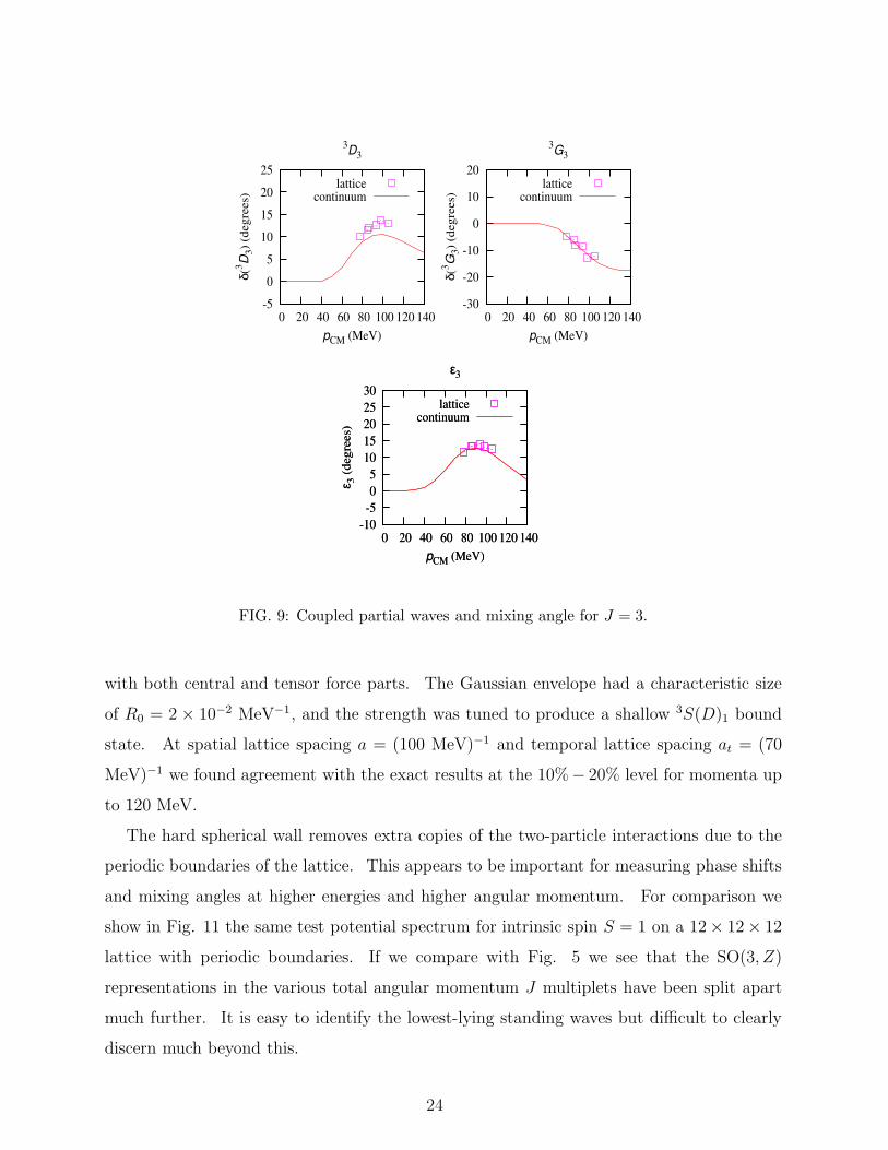
3D3,3G3 partial waves and mixing angle ε3 are shown in Fig. 9. The 3F4,

3H4 partial waves

and mixing angle ε4 are shown in Fig. 10. As before we use Rwall = 10 + ǫ, 9 + ǫ, and 8 + ǫ

21

0

20

40

60

80

100

120

140

160

180

0 20 40 60 80 100 120 140

pCM (MeV)

3S1

δ(3S

1)

(degre

es)

latticecontinuum

-50

-40

-30

-20

-10

0

10

20

0 20 40 60 80 100 120 140

pCM (MeV)

3D1

δ(3D

1)

(degre

es)

latticecontinuum

-40

-30

-20

-10

0

10

20

30

0 20 40 60 80 100 120 140

pCM (MeV)

ε1

ε 1 (

degre

es)

latticecontinuum

-40

-30

-20

-10

0

10

20

30

0 20 40 60 80 100 120 140

pCM (MeV)

ε1

ε 1 (

degre

es)

latticecontinuum

FIG. 7: Coupled partial waves and mixing angle for J = 1. The pairs of points connected by

dotted lines indicate pairs of solutions at k = kI and k = kII .

lattice units. The pairs of points connected by dotted lines indicate pairs of solutions at

k = kI and k = kII . The partial-wave ratios

AIJ−1

AIJ+1

,AII

J−1

AIIJ+1

, (90)

are determined by computing the inner product of the standing wave near the spherical wall

with spherical harmonics.

The lattice results in the coupled channels are somewhat less accurate than the S = 0

results and uncoupled S = 1 results. However they are still within 20% of the exact results

up to momentum 120 MeV. The leading error appears to come from mixing with extraneous

channels due to broken rotational invariance on the lattice. For example the 3S1-3D1

standing waves have a small but non-negligible amount of a 3D3 component. Nevertheless

overall the lattice results are remarkably good for partial-wave mixing at higher total angular

22

0

10

20

30

40

50

0 20 40 60 80 100 120 140

pCM (MeV)

3P2

δ(3P

2)

(degre

es)

latticecontinuum

-40

-30

-20

-10

0

10

20

30

0 20 40 60 80 100 120 140

pCM (MeV)

3F2

δ(3F

2)

(degre

es)

latticecontinuum

-20

-10

0

10

20

30

0 20 40 60 80 100 120 140

pCM (MeV)

ε2

ε 2 (

degre

es)

latticecontinuum

-20

-10

0

10

20

30

0 20 40 60 80 100 120 140

pCM (MeV)

ε2

ε 2 (

degre

es)

latticecontinuum

FIG. 8: Coupled partial waves and mixing angle for J = 2.

momentum.

XI. SUMMARY AND DISCUSSION

We have discussed a general technique for measuring phase shifts and mixing angles for

two-particle scattering on the lattice. In the center-of-mass frame we impose a hard spherical

wall at large fixed radius Rwall. For channels without mixing we identify total angular

momentum J multiplets by the approximate degeneracy of SO(3, Z) representations and

calculate phase shifts from the energies of the spherical standing waves. For channels with

partial-wave mixing, further information is extracted by decomposing the standing wave at

the wall boundary into spherical harmonics. The coupled-channels equations are then solved

to extract the phase shifts and mixing angles. The method was tested by computing phase

shifts and mixing angles for J less than or equal to 4 for an attractive Gaussian potential

23

-5

0

5

10

15

20

25

0 20 40 60 80 100 120 140

pCM (MeV)

3D3

δ(3D

3)

(degre

es)

latticecontinuum

-30

-20

-10

0

10

20

0 20 40 60 80 100 120 140

pCM (MeV)

3G3

δ(3G

3)

(degre

es)

latticecontinuum

-10

-5

0

5

10

15

20

25

30

0 20 40 60 80 100 120 140

pCM (MeV)

ε3

ε 3 (

degre

es)

latticecontinuum

-10

-5

0

5

10

15

20

25

30

0 20 40 60 80 100 120 140

pCM (MeV)

ε3

ε 3 (

degre

es)

latticecontinuum

FIG. 9: Coupled partial waves and mixing angle for J = 3.

with both central and tensor force parts. The Gaussian envelope had a characteristic size

of R0 = 2 × 10−2 MeV−1, and the strength was tuned to produce a shallow 3S(D)1 bound

state. At spatial lattice spacing a = (100 MeV)−1 and temporal lattice spacing at = (70

MeV)−1 we found agreement with the exact results at the 10%− 20% level for momenta up

to 120 MeV.

The hard spherical wall removes extra copies of the two-particle interactions due to the

periodic boundaries of the lattice. This appears to be important for measuring phase shifts

and mixing angles at higher energies and higher angular momentum. For comparison we

show in Fig. 11 the same test potential spectrum for intrinsic spin S = 1 on a 12× 12 × 12

lattice with periodic boundaries. If we compare with Fig. 5 we see that the SO(3, Z)

representations in the various total angular momentum J multiplets have been split apart

much further. It is easy to identify the lowest-lying standing waves but difficult to clearly

discern much beyond this.

24

-4

-2

0

2

4

6

8

10

12

0 20 40 60 80 100 120 140

pCM (MeV)

3F4

δ(3F

4)

(degre

es)

latticecontinuum

-20

-15

-10

-5

0

5

10

0 20 40 60 80 100 120 140

pCM (MeV)

3H4

δ(3H

4)

(degre

es)

latticecontinuum

-5

0

5

10

15

20

25

0 20 40 60 80 100 120 140

pCM (MeV)

ε4

ε 4 (

degre

es)

latticecontinuum

-5

0

5

10

15

20

25

0 20 40 60 80 100 120 140

pCM (MeV)

ε4

ε 4 (

degre

es)

latticecontinuum

FIG. 10: Coupled partial waves and mixing angle for J = 4.

-1

0

1

2

3

4

5

6

7

0 1 2 3

E (

MeV

)

Jz mod 4

S = 1, even parity

A1T1E T2A2

0

1

2

3

4

5

6

7

8

0 1 2 3

E (

MeV

)

Jz mod 4

S = 1, odd parity

FIG. 11: Interacting spectrum for S = 1 standing waves for a 12 × 12 × 12 periodic lattice.

25

The method we have presented can be applied directly to any nonrelativistic effective

theory of point particles on the lattice. There is a long list of interesting few- and many-

body systems one could consider on the lattice. For example one interesting system is that

of atoms and molecules with long-range dipole interactions,

Vdipole-dipole(~r ) ∝ −1

4πr3[3 (r · ~µ1) (r · ~µ2) − ~µ1 · ~µ2] . (91)

There is interest both in magnetic dipole interactions of cold atoms [38, 39, 40, 41, 42] and

electric dipole interactions in cold polar molecules [43, 44, 45, 46]. These spin-changing

interactions are important for determining topological structures of the many-body ground

state as well as practical issues impacting evaporative cooling in magnetic traps.

We will discuss in some detail the application to low-energy nuclear physics in a forth-

coming paper. One important low-energy interaction between nucleons is the exchange of

a virtual pion, producing spin-dependent forces of the form

V1π(~r ) =

(

gA

2fπ

)2

(τ 1 · τ 2)

×

{

m2πe

−mπr

12πr

[

S12(r)

(

1 +3

mπr+

3

(mπr)2

)

+ ~σ1 · ~σ2

]

−1

3~σ1 · ~σ2δ

3(~r )

}

. (92)

Here τ are Pauli matrices in isospin space, mπ is the pion mass, fπ is the pion decay

constant, gA is the nucleon axial charge, and S12(r) is the tensor operator for spin-1/2

particles defined in (3). Recent reviews of literature relating to chiral effective field theory

can be found in [47, 48]. This tensor interaction has some general similarities to that of

the test potential considered here. However the divergent short-distance behavior of the

one-pion exchange potential and other short-distance nucleon-nucleon interactions means

that the lattice spacing plays an essential role in regulating ultraviolet divergences. The

hard spherical wall method we have presented should therefore be useful in determining the

underlying physics of a given lattice action. The singular short-distance interactions are

likely to cause larger breaking of rotational invariance than that found for the bounded test

potential. In such cases it may be useful to include higher-order derivative interactions

specifically designed to cancel lattice artifacts.

26

Acknowledgements

Partial financial support from the Deutsche Forschungsgemeinschaft (SFB/TR 16),

Helmholtz Association (contract number VH-NG-222), and U.S. Department of Energy (DE-

FG02-03ER41260) are gratefully acknowledged. This research is part of the EU Integrated

Infrastructure Initiative in Hadron Physics under contract number RII3-CT-2004-506078.

[1] H. M. Muller, S. E. Koonin, R. Seki, and U. van Kolck, Phys. Rev. C61, 044320 (2000),

nucl-th/9910038.

[2] T. Abe, R. Seki, and A. N. Kocharian, Phys. Rev. C70, 014315 (2004), erratum-ibid. C71

(2005) 059902, nucl-th/0312125.

[3] S. Chandrasekharan, M. Pepe, F. D. Steffen, and U. J. Wiese, Nucl. Phys. Proc. Suppl. 129,

507 (2004), hep-lat/0309093.

[4] S. Chandrasekharan, M. Pepe, F. D. Steffen, and U. J. Wiese, JHEP 12, 035 (2003), hep-

lat/0306020.

[5] D. Lee, B. Borasoy, and T. Schafer, Phys. Rev. C70, 014007 (2004), nucl-th/0402072.

[6] D. Lee and T. Schafer, Phys. Rev. C72, 024006 (2005), nucl-th/0412002.

[7] M. Hamilton, I. Lynch, and D. Lee, Phys. Rev. C71, 044005 (2005), nucl-th/0412014.

[8] R. Seki and U. van Kolck, Phys. Rev. C73, 044006 (2006), nucl-th/0509094.

[9] D. Lee and T. Schafer, Phys. Rev. C73, 015201 (2006), nucl-th/0509017.

[10] D. Lee and T. Schafer, Phys. Rev. C73, 015202 (2006), nucl-th/0509018.

[11] B. Borasoy, H. Krebs, D. Lee, and U.-G. Meißner, Nucl. Phys. A768, 179 (2006), nucl-

th/0510047.

[12] F. de Soto and J. Carbonell (2006), hep-lat/0610040.

[13] B. Borasoy, E. Epelbaum, H. Krebs, D. Lee, and U.-G. Meißner, Eur. Phys. J. A31, 105

(2007), nucl-th/0611087.

[14] D. Lee and R. Thomson, Phys. Rev. C75, 064003 (2007), nucl-th/0701048.

[15] J.-W. Chen and D. B. Kaplan, Phys. Rev. Lett. 92, 257002 (2004), hep-lat/0308016.

[16] M. Wingate (2005), cond-mat/0502372.

[17] A. Bulgac, J. E. Drut, and P. Magierski, Phys. Rev. Lett. 96, 090404 (2006), cond-

27

mat/0505374.

[18] D. Lee, Phys. Rev. B73, 115112 (2006), cond-mat/0511332.

[19] E. Burovski, N. Prokofev, B. Svistunov, and M. Troyer, Phys. Rev. Lett. 96, 160402 (2006),

cond-mat/0602224.

[20] E. Burovski, N. Prokofev, B. Svistunov, and M. Troyer, New J. Phys. 8, 153 (2006), cond-

mat/0605350.

[21] D. Lee, Phys. Rev. B75, 134502 (2007), cond-mat/0606706.

[22] M. Luscher, Commun. Math. Phys. 104, 177 (1986).

[23] M. Luscher, Commun. Math. Phys. 105, 153 (1986).

[24] M. Luscher, Nucl. Phys. B354, 531 (1991).

[25] X. Li and C. Liu, Phys. Lett. B587, 100 (2004), hep-lat/0311035.

[26] X. Feng, X. Li, and C. Liu, Phys. Rev. D70, 014505 (2004), hep-lat/0404001.

[27] S. R. Beane, P. F. Bedaque, A. Parreno, and M. J. Savage, Phys. Lett. B585, 106 (2004),

hep-lat/0312004.

[28] K. Rummukainen and S. A. Gottlieb, Nucl. Phys. B450, 397 (1995), hep-lat/9503028.

[29] C. H. Kim, C. T. Sachrajda, and S. R. Sharpe, Nucl. Phys. B727, 218 (2005), hep-lat/0507006.

[30] I. Sato and P. F. Bedaque (2007), hep-lat/0702021.

[31] S. Sasaki and T. Yamazaki, Phys. Rev. D74, 114507 (2006), hep-lat/0610081.

[32] S. R. Beane, W. Detmold, and M. J. Savage (2007), arXiv:0707.1670 [hep-lat].

[33] R. C. Johnson, Phys. Lett. B114, 147 (1982).

[34] C. Lanczos, J. Res. Nat. Bur. Stand. 45, 255 (1950).

[35] H. P. Stapp, T. J. Ypsilantis, and N. Metropolis, Phys. Rev. 105, 302 (1957).

[36] J. M. Blatt and L. C. Biedenharn, Phys. Rev. 86, 399 (1952).

[37] J. M. Blatt and L. C. Biedenharn, Rev. Mod. Phys. 24, 258 (1952).

[38] C. A. Regal, C. Ticknor, J. L. Bohn, and D. S. Jin, Phys. Rev. Lett. 90, 053201 (2003),

cond-mat/0209071v1.

[39] J. Zhang, E. G. M. van Kempen, T. Bourdel, L. Khaykovich, J. Cubizolles, F. Chevy, M. Te-

ichmann, L. Tarruell, S. J. J. M. F. Kokkelmans, and C. Salomon, Phys. Rev. A 70, 030702(R)

(2004).

[40] C. H. Schunck, M. W. Zwierlein, C. A. Stan, S. M. F. Raupach, W. Ketterle, A. Simoni,

E. Tiesinga, C. J. Williams, and P. S. Julienne, Phys. Rev. A 71, 045601 (2005), cond-

28

mat/0407373.

[41] J. P. Gaebler, J. T. Stewart, J. L. Bohn, and D. S. Jin (2007), cond-mat/0703087.

[42] J. G. E. Harris, S. V. Nguyen, S. C. Doret, W. Ketterle, and J. M. Doyle (2007),

arXiv.org:0705.0713.

[43] J. Doyle, B. Friedrich, R. V. Krems, and F. Masnou-Seeuws, Eur. Phys. J. D31, 149 (2004),

physics/0505201.

[44] K. Gunter, T. Stoferle, H. Moritz, M. Kohl, and T. Esslinger, Phys. Rev. Lett. 95, 230401

(2005), cond-mat/0507632.

[45] A. Micheli, G. K. Brennen, and P. Zoller, Nat. Phys. 2, 341 (2006), quant-ph/0512222v2.

[46] G. K. Brennen, A. Micheli, and P. Zoller, New J. Phys. 9, 138 (2007), quant-ph/0612180.

[47] P. F. Bedaque and U. van Kolck, Ann. Rev. Nucl. Part. Sci. 52, 339 (2002), nucl-th/0203055.

[48] E. Epelbaum, Prog. Part. Nucl. Phys. 57, 654 (2006), nucl-th/0509032.

29