177
Images from Nicolás García Rosa (Supaero Ph.D) Two-phase Flows in Combustion Systems Gérard Lavergne SUPAERO, ONERA
| Date post: | 02-Jun-2018 |
| Category: |
Documents |
| Upload: | julinavia3482 |
| View: | 220 times |
| Download: | 1 times |

8/10/2019 Two phase flow in combustion system
http://slidepdf.com/reader/full/two-phase-flow-in-combustion-system 1/177
Images from Nicolás García Rosa (Supaero Ph.D)
Two-phase Flowsin Combustion
Systems
Gérard Lavergne
SUPAERO, ONERA

8/10/2019 Two phase flow in combustion system
http://slidepdf.com/reader/full/two-phase-flow-in-combustion-system 2/177
CHAPTER I: INTRODUCTION TO COMBUSTION AND FLAMES IN INDUSTRY ............ .............. ..... 4
I. INTRODUCTION........................................................................................................................................... 5 II. COMBUSTION AND FLAMES IN INDUSTRY AND IN THE NATURE. ...................................................................... 8
CHAPTERII: INTRODUCTION TO TWO PHASE FLOWS........................................................................29 CHAPTER III: DEFINITIONS AND CLASSIFICATION OF THE DIFFERENT RÉGIMES OF TWOPHASE FLOWS...................................................................................................................................................33
I : DENSITY AND MASS FRACTION.......................................................................................................................34 II RELAXATION TIME..........................................................................................................................................36
III. DILUTED AND DENSE TWO PHASE FLOWS .....................................................................................................39 CHAPTER IV: DIFFERENT APPROACHES FOR TWO PHASE FLOWS NUMERICALSIMULATION .....................................................................................................................................................41
I. GASEOUS PHASE NUMERICAL SIMULATION : ...................................................................................................42 I.1 Introduction....... .............. ............. ............ .............. ............. .............. ............ ............. .............. .............. .42 I.2 Scales and main characteristics of the turbulence ............ ............. .............. ............. ............ .............. ....42 Kinetic energy of turbulence.........................................................................................................................44 Spectrum of the length scales of the turbulence ...........................................................................................44
RANS .............. ............ .............. ............. ............ .............. ............. .............. ............ ............. .............. .............. .46 LES....................................................................................................................................................................46 DNS...................................................................................................................................................................46 II. TWO APPROACHES FOR TWO PHASE FLOW MODELING....................................................................................47
II.1 Euler/Euler approach ........................ ............ .............. ............. ............ .............. ............. .............. ........47 II.2 Euler/Lagrange approach............... .............. ............. ............ .............. ............. .............. ............ ...........49
CHAPTER V: SPRAY FORMATION ..............................................................................................................51 I COMBUSTION CHAMBER AND INJECTION SYSTEM.............................................................................................52 SPRAY MEASUREMENT ......................................................................................................................................55 II PRIMARY AND SECONDARY LIQUID SHEET BEAK UP ........................................................................................56
Atomisation...... .............. ............. ............ .............. ............. .............. ............ .............. ............. .............. ........56 Secondary break-up......................................................................................................................................58
III, DROPLET SIZE,DEFINITIONS, NON DIMENSIONAL NUMBERS, DIFFÉRENT INJECTION SYSTEMS........................61 III, DROPLET SIZE,DEFINITIONS, NON DIMENSIONAL NUMBERS, DIFFÉRENT INJECTION SYSTEMS........................62
Size distributions ..........................................................................................................................................62 Mean size............... ............ ............. .............. ............. ............. ............. .............. ............. ............ .............. ....62 Distribution function: ............. ............ .............. ............. .............. ............ .............. ............. ............ ..............62
CHAPTER VI: TURBULENT DISPERSION OF THE LIQUID PHASE.....................................................64 I. DRAG COEFFICIENT OF A SPHERICAL PARTICLE (OR DROPLET) ........................................................................65
Drag coefficient for subsonic compressible flows .............. ............. ............ .............. ............. .............. ........66 Drag coefficient for supersonic compressive flows ............ ............. ............ .............. ............. .............. ........66 Drag coefficient in rarefied gases ............ ............ .............. ............. ............ .............. ............. .............. ........67
II. TURBULENT PARTICLES (OR DROPLETS) DISPERSION .....................................................................................69 CHAPTER VII: DROPLET EVAPORATION AND COMBUSTION...........................................................74
EVAPORATION MODEL FOR AN ISOLATED DROPLET............................................................................................75 Liquid phase calculation/Droplet heating ............ .............. ............. ............ .............. ............. .............. ........76 I.1 Isolated droplet evaporation without convection ............ ............ .............. ............. .............. ............ .......77 I.2 Variable physical properties ............ .............. ............. ............ .............. ............. ............ .............. ...........81 I.3 Convection correction.............. ............ .............. ............. ............ .............. ............. .............. ............ .......82
I.4 LIQUID PHASE MODEL ...................................................................................................................................84 • D
2model : ...........................................................................................................................................84
• Infinite Conductivity.......... .............. ............ .............. ............. ............ .............. ............. .............. ........84 • Limited conduction............... ............ .............. ............. ............ .............. ............. .............. ............ .......85 • Effective conduction.... ............. ............ .............. ............. .............. ............ ............. .............. ............. ..85 Validation .............. ............ ............. .............. ............. ............. ............. .............. ............. ............ .............. ....86 Continuity equation for species in spherical coordinates.............................................................................86 Combustion rate computation.......................................................................................................................89 Flame position ............. ............. ............. .............. ............. ............ .............. ............. ............ .............. ...........90 - Temperature profile....................................................................................................................................90 - Combustion time.........................................................................................................................................91
QUASI-STEADY THEORY OF AN ISOLATED DROPLET BURNING ............................................................................92 CHAPTER VIII DENSE SPRAYS...................................................................................................................102
INTRODUCTION ................................................................................................................................................105
8/10/2019 Two phase flow in combustion system
http://slidepdf.com/reader/full/two-phase-flow-in-combustion-system 3/177
EXPERIMENTAL SETUP .....................................................................................................................................106 Droplet Generator............ ............. ............ .............. ............. ............ .............. ............. .............. ............ .....106 Electrostatic Droplet Deflector ..................... .............. ............. .............. ............ ............. .............. .............106 Measuring techniques............. ............ .............. ............. .............. ............ .............. ............. ............ ............106 Droplet Size Measurements............ .............. ............. ............. ............. .............. ............. ............ .............. ..107 Droplet Temperature Measurements ............ ............. ............. ............. .............. ............. ............ .............. ..107 Droplet Velocity Measurements .................... .............. ............. .............. ............ ............. .............. .............107 CARS Thermometry .............. ............. ............ .............. ............. .............. ............ ............. .............. .............108
RESULTS AND DISCUSSION ...............................................................................................................................108 Drag Coefficient under Non Evaporating Conditions:.. .............. ............ .............. ............. ............ ............108 Reacting Conditions ...................... ............ .............. ............. ............ .............. ............. .............. ............ .....109
CHAPTER IX : DROPLET WALL INTERACTION......... ............ .............. ............. ............ .............. .........117 DROPLET BEHAVIOR ON A HOT WALL ...............................................................................................................118 FIRST CLASSIFICATION (PHD C. AMIEL SUPAERO) .......................................................................................122 SECOND CLASSIFICATION (P. VILLEDIEU) ........................................................................................................122
CHAPTER IX: EULER-LAGRANGE APPROACH, TWO WAY COUPLING ............. .............. .............126 THE PARTICLE SOURCE IN CELL MODEL (PSICM) FOR GAS DROPLET FLOWS ................................................128 BASIC CONCEPT ...............................................................................................................................................128 SOURCE TERMS ................................................................................................................................................129
CHAPTER X : EXAMPLES OF STUDIED CONFIGURATIONS..............................................................133 DROPLET TRAJECTORY IN A TURBULENT FLOW................................................................................................134 DUMP COMBUSTOR [11] ..................................................................................................................................134 LEAN PREMIXER PREVAPORISER MODULE [12].................................................................................................135 MODELLING OF THE TWO PHASE FLOW IN SOLID ROCKET MOTORS [13,14]......................................................135
REFERENCES...................................................................................................................................................139 ACKNOWLEDGEMENTS...............................................................................................................................153 EXERCISES.......................................................................................................................................................154
EXERCISE 1: LIQUID SHEET DISINTEGRATION ...................................................................................................155 EXERCISE 2: DROPLET EVAPORATION...............................................................................................................158 EX 3 : STABILITY OF A TURBOJET COMBUSTION CHAMBER...............................................................................159 EXERCISE 4 : COMBUSTION CHAMBER DESIGN .................................................................................................160 EXERCISE 5: DROPLET TRAJECTORIES IN AN ACOUSTIC FIELD ..........................................................................169
8/10/2019 Two phase flow in combustion system
http://slidepdf.com/reader/full/two-phase-flow-in-combustion-system 4/177
Chapter I: Introduction to Combustion andflames in industry
8/10/2019 Two phase flow in combustion system
http://slidepdf.com/reader/full/two-phase-flow-in-combustion-system 5/177
8/10/2019 Two phase flow in combustion system
http://slidepdf.com/reader/full/two-phase-flow-in-combustion-system 6/177
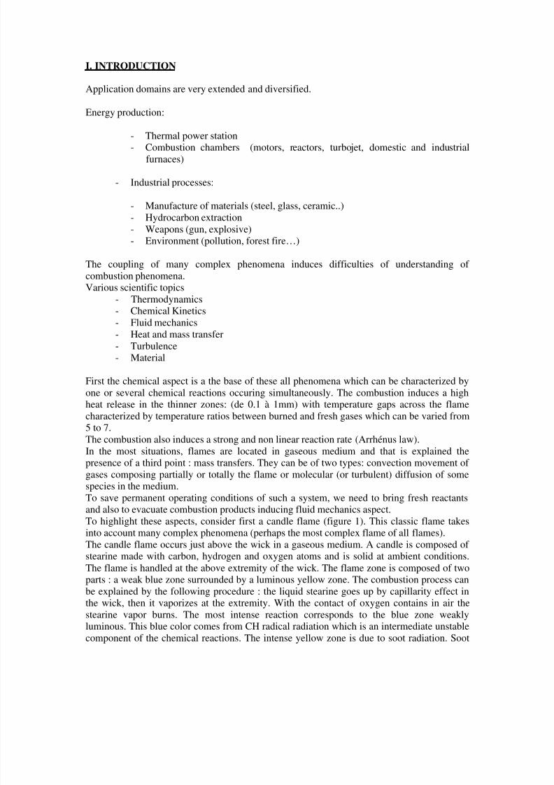
are carbon particles, C, which collide. The presence of these particles is due to a non completecombustion. That is means that oxygen is lacking to burn all the available amount of fuel. Incontrary soot emits a lot of light, thanks to this particle emission the candle can lighteverybody.!!The candle light comes from a radiative thermal transfer. The thermal transfers also producesthe liquefaction of the stearine at the top of the candle by conduction in the wick and by
radiationAt the last, the fluid mechanics is necessary to mix vapor and air. The natural convectioninduced by the heat release entrains fresh air along the flame necessary for the combustionand to evacuate the combustion products (CO 2 , H 2 O, carbon particles).
Figure 1 [1] Different physical aspects in a candle flame
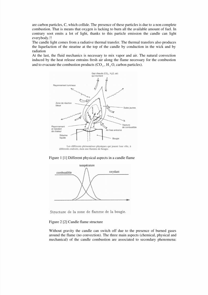
Figure 2 [2] Candle flame structure
Without gravity the candle can switch off due to the presence of burned gasesaround the flame (no convection). The three main aspects (chemical, physical andmechanical) of the candle combustion are associated to secondary phenomena:
8/10/2019 Two phase flow in combustion system
http://slidepdf.com/reader/full/two-phase-flow-in-combustion-system 7/177
liquefaction, evaporation, nucleation and collision of soot particles. The heatconduction in the porous wick and the ascension of the liquid stearine along thewick are also some physical processes participating to the flame. The figure 2shows a simplified scheme of the flame structure. The zone where the chemicalreactions occur shares a gaseous medium where gases are oxidizer (outside) and agaseous medium (reductor, inside).
This kind of flame is called diffusion flame (mass transfer by molecular diffusion)or non-premixed flames.
- Premixed laminar flames
Two main combustion regimes can be encountered: the diffusion flame and thepremixed flame. In this last case the oxidizer and the fuel are mix upstream thecombustion zone..
Example of premixed flame
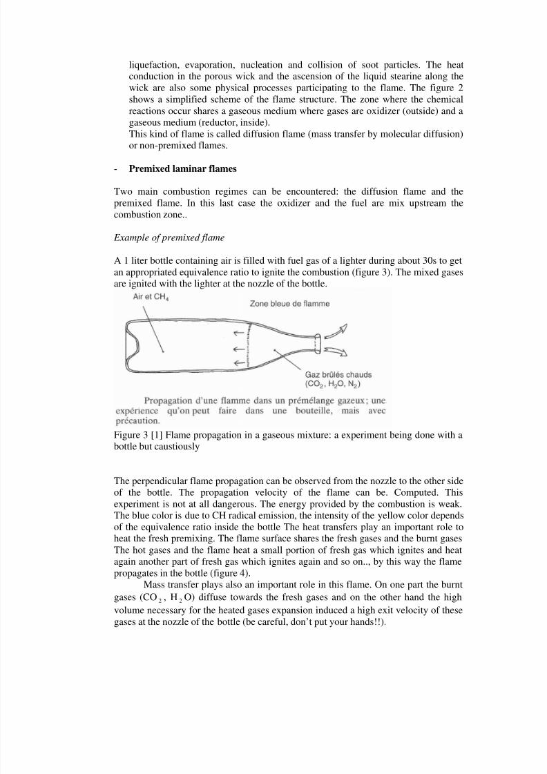
A 1 liter bottle containing air is filled with fuel gas of a lighter during about 30s to get
an appropriated equivalence ratio to ignite the combustion (figure 3). The mixed gasesare ignited with the lighter at the nozzle of the bottle.
Figure 3 [1] Flame propagation in a gaseous mixture: a experiment being done with abottle but caustiously
The perpendicular flame propagation can be observed from the nozzle to the other sideof the bottle. The propagation velocity of the flame can be. Computed. Thisexperiment is not at all dangerous. The energy provided by the combustion is weak.The blue color is due to CH radical emission, the intensity of the yellow color dependsof the equivalence ratio inside the bottle The heat transfers play an important role to
heat the fresh premixing. The flame surface shares the fresh gases and the burnt gasesThe hot gases and the flame heat a small portion of fresh gas which ignites and heatagain another part of fresh gas which ignites again and so on.., by this way the flamepropagates in the bottle (figure 4).
Mass transfer plays also an important role in this flame. On one part the burntgases (CO 2 , H 2 O) diffuse towards the fresh gases and on the other hand the highvolume necessary for the heated gases expansion induced a high exit velocity of thesegases at the nozzle of the bottle (be careful, don’t put your hands!!).

8/10/2019 Two phase flow in combustion system
http://slidepdf.com/reader/full/two-phase-flow-in-combustion-system 8/177
Figure 4 [2] Premixed laminar flame strucure
II. COMBUSTION AND FLAMES IN INDUSTRY AND IN THE NATURE.
The synoptic presents a classification of different practical systems of combustion following
the type reactant injection types (diffusion or premixed).
Figure 5: Different types of flame
8/10/2019 Two phase flow in combustion system
http://slidepdf.com/reader/full/two-phase-flow-in-combustion-system 9/177
- motors
Two kinds of motors
• Airbreathing using oxygen of the air.
• no airbreathing (rocket motors for example), oxygen comes from otherssources.
Different types of airbreathing motors:
Piston engine ignites by a spark plug or diesel The physical processes are so complex that is very difficult to predict thecombustion chamber performance from a numerical computation. However thenumerical simulation is used to reduce the number of experimental tests and toreduce the cost.Many empirical approaches are yet used for combustion chamber development.For example in France, the Renault society has developed only three motors
between 1960 and 1980.The actual motivation in the domain of research is to improve theunderstanding of the physics of this hind of reacting two phase flows, todevelop new models to get some predictive tools for performancescomputation. From 1960, the car consumption has been divided by two, thevolume of the cylinder has been reduced from some liters to 1000 cm3, thepower has increased and the weight reduced.
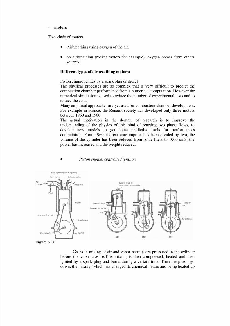
• Piston engine, controlled ignition
Figure 6 [3]
Gases (a mixing of air and vapor petrol). are pressured in the cylinderbefore the valve closure.This mixing is then compressed, heated and thenignited by a spark plug and burns during a certain time. Then the piston godown, the mixing (which has changed its chemical nature and being heated up
8/10/2019 Two phase flow in combustion system
http://slidepdf.com/reader/full/two-phase-flow-in-combustion-system 10/177
to 2500 or 2700K) is then expanded and cooled and finally exhaust when theexhaust valves are open and the piston go up. The ignition appears for a crankangle about of 20 before the high dead point and the end of combustion of thetotal volume of gas contained in the cylinder corresponds to about a crankangle of 20° after the high dead point.
Example : If the rotation velocity of a motor is 3000t/mn, the combustion delay isabout : (40/360)*(60/3000) seconds, about 2 milliseconds ; this delay is enough longfor the chemical reactions.
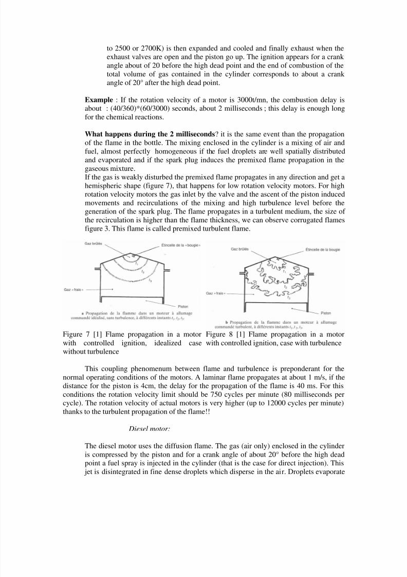
What happens during the 2 milliseconds? it is the same event than the propagationof the flame in the bottle. The mixing enclosed in the cylinder is a mixing of air andfuel, almost perfectly homogeneous if the fuel droplets are well spatially distributedand evaporated and if the spark plug induces the premixed flame propagation in thegaseous mixture.If the gas is weakly disturbed the premixed flame propagates in any direction and get ahemispheric shape (figure 7), that happens for low rotation velocity motors. For highrotation velocity motors the gas inlet by the valve and the ascent of the piston induced
movements and recirculations of the mixing and high turbulence level before thegeneration of the spark plug. The flame propagates in a turbulent medium, the size ofthe recirculation is higher than the flame thickness, we can observe corrugated flamesfigure 3. This flame is called premixed turbulent flame.
Figure 7 [1] Flame propagation in a motorwith controlled ignition, idealized casewithout turbulence
Figure 8 [1] Flame propagation in a motorwith controlled ignition, case with turbulence
This coupling phenomenum between flame and turbulence is preponderant for thenormal operating conditions of the motors. A laminar flame propagates at about 1 m/s, if thedistance for the piston is 4cm, the delay for the propagation of the flame is 40 ms. For thisconditions the rotation velocity limit should be 750 cycles per minute (80 milliseconds per
cycle). The rotation velocity of actual motors is very higher (up to 12000 cycles per minute)thanks to the turbulent propagation of the flame!!
Diesel motor:
The diesel motor uses the diffusion flame. The gas (air only) enclosed in the cylinderis compressed by the piston and for a crank angle of about 20° before the high deadpoint a fuel spray is injected in the cylinder (that is the case for direct injection). This
jet is disintegrated in fine dense droplets which disperse in the air. Droplets evaporate
8/10/2019 Two phase flow in combustion system
http://slidepdf.com/reader/full/two-phase-flow-in-combustion-system 11/177
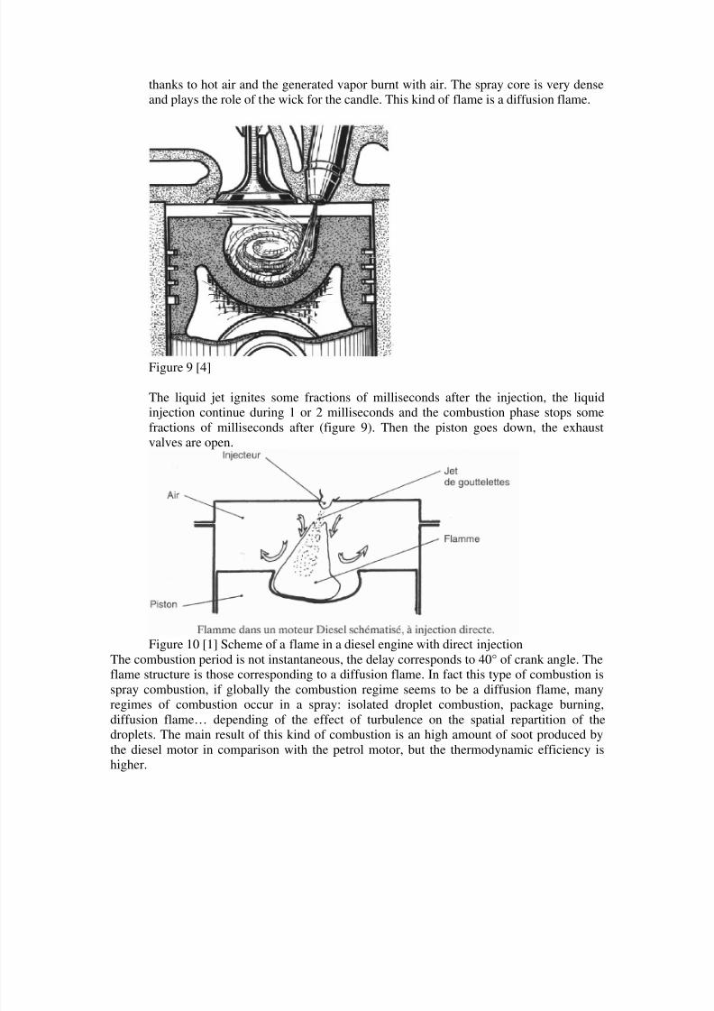
thanks to hot air and the generated vapor burnt with air. The spray core is very denseand plays the role of the wick for the candle. This kind of flame is a diffusion flame.
Figure 9 [4]
The liquid jet ignites some fractions of milliseconds after the injection, the liquidinjection continue during 1 or 2 milliseconds and the combustion phase stops somefractions of milliseconds after (figure 9). Then the piston goes down, the exhaustvalves are open.
Figure 10 [1] Scheme of a flame in a diesel engine with direct injectionThe combustion period is not instantaneous, the delay corresponds to 40° of crank angle. Theflame structure is those corresponding to a diffusion flame. In fact this type of combustion isspray combustion, if globally the combustion regime seems to be a diffusion flame, many
regimes of combustion occur in a spray: isolated droplet combustion, package burning,diffusion flame… depending of the effect of turbulence on the spatial repartition of thedroplets. The main result of this kind of combustion is an high amount of soot produced bythe diesel motor in comparison with the petrol motor, but the thermodynamic efficiency ishigher.
8/10/2019 Two phase flow in combustion system
http://slidepdf.com/reader/full/two-phase-flow-in-combustion-system 12/177
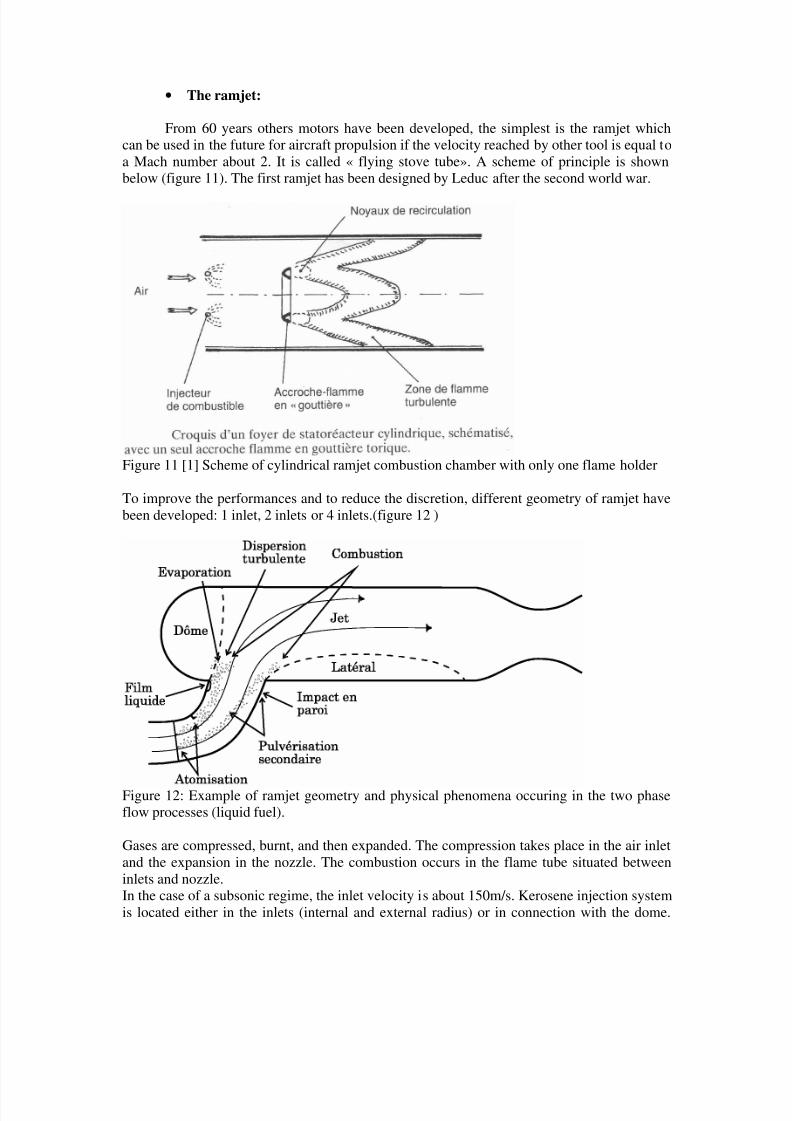
• The ramjet:
From 60 years others motors have been developed, the simplest is the ramjet whichcan be used in the future for aircraft propulsion if the velocity reached by other tool is equal toa Mach number about 2. It is called « flying stove tube». A scheme of principle is shownbelow (figure 11). The first ramjet has been designed by Leduc after the second world war.
Figure 11 [1] Scheme of cylindrical ramjet combustion chamber with only one flame holder
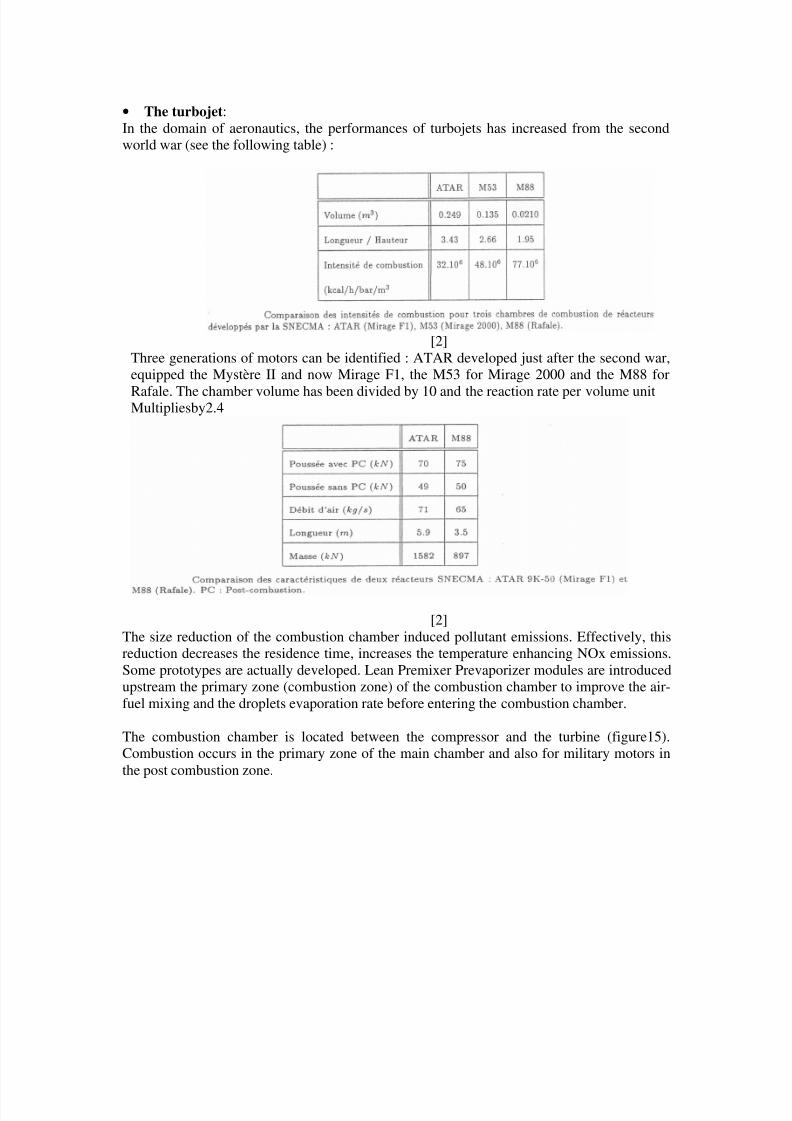
To improve the performances and to reduce the discretion, different geometry of ramjet havebeen developed: 1 inlet, 2 inlets or 4 inlets.(figure 12 )
Figure 12: Example of ramjet geometry and physical phenomena occuring in the two phaseflow processes (liquid fuel).
Gases are compressed, burnt, and then expanded. The compression takes place in the air inletand the expansion in the nozzle. The combustion occurs in the flame tube situated betweeninlets and nozzle.In the case of a subsonic regime, the inlet velocity is about 150m/s. Kerosene injection systemis located either in the inlets (internal and external radius) or in connection with the dome.

8/10/2019 Two phase flow in combustion system
http://slidepdf.com/reader/full/two-phase-flow-in-combustion-system 13/177
The liquid fuel is generated in this case directly in the flame tube.The fuel is disintegratedthen evaporated at the entry of the combustion zone. The combustion chamber performancesare depending on disintegration quality but also of the position of the injection devices whichinfluences the spatial repartition of the equivalence ratio.These geometries are defined in order to generate several recirculating zones to attach theflame. We can distinguish on the previous figure three main zones, one between the inlets
called “dome” which is a very mixed zone piloting the stability of the combustion chamber,the other called “lateral recirculating zone” which is a non well mixed zone and then the jetwithout recirculation.In the frame of a global approach a network of elementary reactors is considered, the two
first zones are modeled as well stirred reactors and the last as piston reactor. The maincharacteristics of these reactors (volume, residence time, airflow rate, fuel flow rate…) have adeterminant influence on the ramjet performances. To improve the turbulence level inside therecirculating zones some obstacles are placed in the inlet. Heat and mass transfer occur insidethese zones, and the combustion in maintained if the residence time is enough high or if theair velocity is low. The flame regime observed is not diffusion or premixed flame. It is calledcombustion zone.These zones produced permanently hot gases in the main flow and then thecombustion propagates between these different zones.(figure 13).
Figure 13 [1] Some details on flame stabilization from recirculating kernels behind the flameholder
In the flame tube the mean air velocity is about 50m/s.One example of numerical simulation of the reactive unsteady two phase flows is shownbelow for a simplified ramjet configuration.
Figure 14: Example of numerical simulation of reacting two phase flow inside a dumpconfiguration[5]
The ramjet propulsion type is often uses in the military domain, for missile propulsion butactually some recent researches are lead for plane propulsion for the cruise flight (scramjet).
8/10/2019 Two phase flow in combustion system
http://slidepdf.com/reader/full/two-phase-flow-in-combustion-system 14/177
• The turbojet:In the domain of aeronautics, the performances of turbojets has increased from the secondworld war (see the following table) :
[2]Three generations of motors can be identified : ATAR developed just after the second war,equipped the Mystère II and now Mirage F1, the M53 for Mirage 2000 and the M88 for
Rafale. The chamber volume has been divided by 10 and the reaction rate per volume unitMultipliesby2.4
[2]The size reduction of the combustion chamber induced pollutant emissions. Effectively, thisreduction decreases the residence time, increases the temperature enhancing NOx emissions.Some prototypes are actually developed. Lean Premixer Prevaporizer modules are introducedupstream the primary zone (combustion zone) of the combustion chamber to improve the air-fuel mixing and the droplets evaporation rate before entering the combustion chamber.
The combustion chamber is located between the compressor and the turbine (figure15).Combustion occurs in the primary zone of the main chamber and also for military motors inthe post combustion zone.

8/10/2019 Two phase flow in combustion system
http://slidepdf.com/reader/full/two-phase-flow-in-combustion-system 15/177
Figure 15: Scheme of an aeronautic reactor
An actual combustion chamber configuration is presented below:
Figure 16: Scheme of a combustion chamber sector
8/10/2019 Two phase flow in combustion system
http://slidepdf.com/reader/full/two-phase-flow-in-combustion-system 16/177
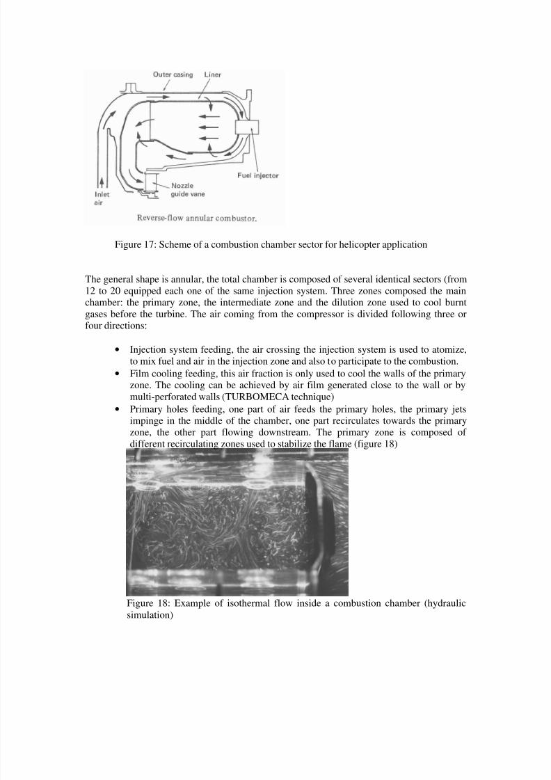
Figure 17: Scheme of a combustion chamber sector for helicopter application
The general shape is annular, the total chamber is composed of several identical sectors (from12 to 20 equipped each one of the same injection system. Three zones composed the mainchamber: the primary zone, the intermediate zone and the dilution zone used to cool burntgases before the turbine. The air coming from the compressor is divided following three orfour directions:
• Injection system feeding, the air crossing the injection system is used to atomize,to mix fuel and air in the injection zone and also to participate to the combustion.
• Film cooling feeding, this air fraction is only used to cool the walls of the primaryzone. The cooling can be achieved by air film generated close to the wall or bymulti-perforated walls (TURBOMECA technique)
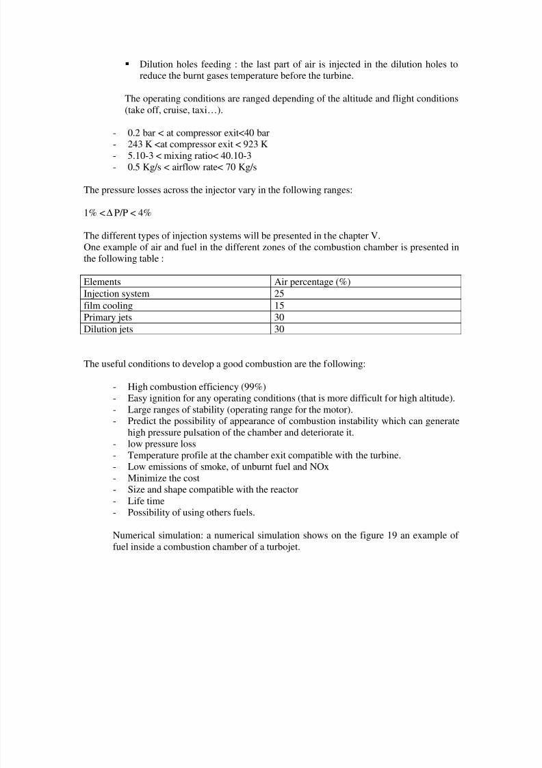
• Primary holes feeding, one part of air feeds the primary holes, the primary jetsimpinge in the middle of the chamber, one part recirculates towards the primaryzone, the other part flowing downstream. The primary zone is composed ofdifferent recirculating zones used to stabilize the flame (figure 18)
Figure 18: Example of isothermal flow inside a combustion chamber (hydraulicsimulation)
8/10/2019 Two phase flow in combustion system
http://slidepdf.com/reader/full/two-phase-flow-in-combustion-system 17/177
Dilution holes feeding : the last part of air is injected in the dilution holes toreduce the burnt gases temperature before the turbine.
The operating conditions are ranged depending of the altitude and flight conditions(take off, cruise, taxi…).
- 0.2 bar < at compressor exit<40 bar- 243 K <at compressor exit < 923 K- 5.10-3 < mixing ratio< 40.10-3- 0.5 Kg/s < airflow rate< 70 Kg/s
The pressure losses across the injector vary in the following ranges:
1% < ∆ P/P < 4%
The different types of injection systems will be presented in the chapter V.One example of air and fuel in the different zones of the combustion chamber is presented inthe following table :
Elements Air percentage (%)Injection system 25film cooling 15Primary jets 30Dilution jets 30
The useful conditions to develop a good combustion are the following:
- High combustion efficiency (99%)- Easy ignition for any operating conditions (that is more difficult for high altitude).- Large ranges of stability (operating range for the motor).- Predict the possibility of appearance of combustion instability which can generate
high pressure pulsation of the chamber and deteriorate it.- low pressure loss- Temperature profile at the chamber exit compatible with the turbine.- Low emissions of smoke, of unburnt fuel and NOx- Minimize the cost- Size and shape compatible with the reactor- Life time- Possibility of using others fuels.
Numerical simulation: a numerical simulation shows on the figure 19 an example offuel inside a combustion chamber of a turbojet.

8/10/2019 Two phase flow in combustion system
http://slidepdf.com/reader/full/two-phase-flow-in-combustion-system 18/177
Figure 19: Example of fuel repartition in a combustion chamber of turbojet (numericalsimulation [6])
• Post-combustion zone
Figure 20 [2] Scheme of post combustion chamber
The post combustion zone (PC) or reheat zone is a second combustion chamber locateddownstream the turbine. It exists only on military aircraft, except on Concorde which usespost combustion to get supersonic regime. This zone is feed by burnt gases coming from themain chamber, expanded in the turbine and by the secondary air flux coming directly from thecompressor. These two fluxes must be optimized to get the best possible combustion. Theflame is stabilized by the flame holder composed of concentric rings. The kerosene is injectedby very simple injector.
The operating conditions are the following :
0.3 bar < pressure < 6 bar800 K < upstream mean temperature <900 K40. 10-3 < mixing ratio< 68. 10-31 Kg/s < air flow rate < 100 kg/s
8/10/2019 Two phase flow in combustion system
http://slidepdf.com/reader/full/two-phase-flow-in-combustion-system 19/177
Combustion instabilities are often encountered in the post combustion zone linked to thepresence of flow instabilities in the recirculating zone behind the flame holder. A passivecontrol is generally applies to reduce these instabilities. The ignition of the post combustionzone must be performed just at the starting. Noise and discretion are also some actual researchtopics.
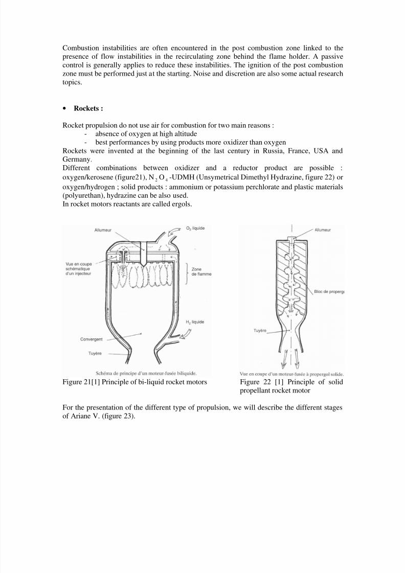
• Rockets :
Rocket propulsion do not use air for combustion for two main reasons :- absence of oxygen at high altitude- best performances by using products more oxidizer than oxygen
Rockets were invented at the beginning of the last century in Russia, France, USA andGermany.Different combinations between oxidizer and a reductor product are possible :oxygen/kerosene (figure21), N 2 O 4 -UDMH (Unsymetrical Dimethyl Hydrazine, figure 22) oroxygen/hydrogen ; solid products : ammonium or potassium perchlorate and plastic materials(polyurethan), hydrazine can be also used.In rocket motors reactants are called ergols.
Figure 21[1] Principle of bi-liquid rocket motors Figure 22 [1] Principle of solidpropellant rocket motor
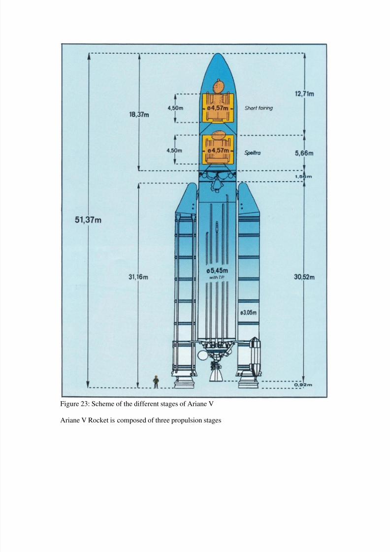
For the presentation of the different type of propulsion, we will describe the different stagesof Ariane V. (figure 23).
8/10/2019 Two phase flow in combustion system
http://slidepdf.com/reader/full/two-phase-flow-in-combustion-system 20/177
Figure 23: Scheme of the different stages of Ariane V
Ariane V Rocket is composed of three propulsion stages
8/10/2019 Two phase flow in combustion system
http://slidepdf.com/reader/full/two-phase-flow-in-combustion-system 21/177
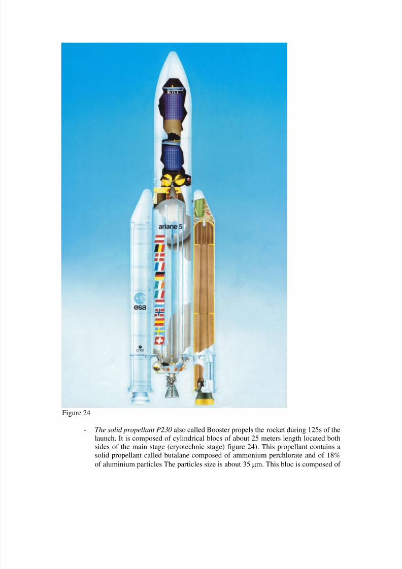
Figure 24
- The solid propellant P230 also called Booster propels the rocket during 125s of thelaunch. It is composed of cylindrical blocs of about 25 meters length located bothsides of the main stage (cryotechnic stage) figure 24). This propellant contains asolid propellant called butalane composed of ammonium perchlorate and of 18%of aluminium particles The particles size is about 35 µm. This bloc is composed of

8/10/2019 Two phase flow in combustion system
http://slidepdf.com/reader/full/two-phase-flow-in-combustion-system 22/177
three segments S1, S2 et S3 separated by thermal protections. The igniter is locatedat the top of segment S3, the nozzle is an integrated nozzle in order to point it up to7°. The combustion takes place at the surface of the grain. The regression surfacevelocity is about a few millimeters per second and the gas flow rate is proportionalto the burnt surface. The gas flow rate being controlled, the nozzle section beingfixed, the chamber pressure and the thrust are controlled too. The internal pressure
is of 50 bar and the temperature about 3500 K- This propellant behavior is like a close cavity. It is composed of two waterproofwalls and a sonic nozzle. Instability problems can occur from the coupling betweenacoustic modes of the chamber and aerodynamics instabilities coming fromthermal protection.Some aluminium particles contained in the grain agglomerate after their fusion andcontinue their burning in the burnt gases. The aluminium particle combustion isnot yet well known and the modeling is very difficult. Studies linked inlaboratories show a deposition of alumina slag on the aluminium particle givingafter combustion a alumina residue size about 60 µm. After 60S of the launch thezone around the nozzle do not contain any grain and a recirculating zone appearsand freeze some alumina droplets. At the end of the launch 2 or 3 tons of alumina
is deposited around the nozzle. This aspect reduces the performances of thelauncher.These two phenomena: instability and slag in the solid propellant are well studiedin France and in USA..One example of computation on scale 1is presented below :
Figure 25 [7] Example of computation of reactive flow inside the booster
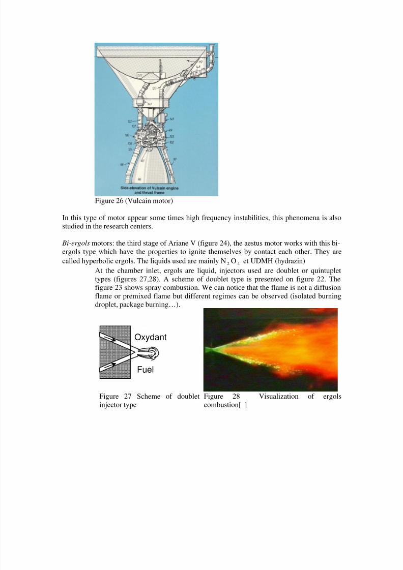
The second stage: the cryotechnic stage
The geometry of this kind of chamber is simple. Upstream the chamber isequipped of coaxial injectors, liquid oxygen is injected at the center and gaseoushydrogen at the periphery. Hydrogen is generated with a velocity about 200m/sand disintegrates liquid oxygen to create a spray and a igniter generates thecombustion. Downstream, the nozzle accelerates the burnt gases to provide thethrust of the motor.
8/10/2019 Two phase flow in combustion system
http://slidepdf.com/reader/full/two-phase-flow-in-combustion-system 23/177
Figure 26 (Vulcain motor)
In this type of motor appear some times high frequency instabilities, this phenomena is alsostudied in the research centers.
Bi-ergols motors: the third stage of Ariane V (figure 24), the aestus motor works with this bi-ergols type which have the properties to ignite themselves by contact each other. They arecalled hyperbolic ergols. The liquids used are mainly N 2 O 4 et UDMH (hydrazin)
At the chamber inlet, ergols are liquid, injectors used are doublet or quintuplettypes (figures 27,28). A scheme of doublet type is presented on figure 22. Thefigure 23 shows spray combustion. We can notice that the flame is not a diffusion
flame or premixed flame but different regimes can be observed (isolated burningdroplet, package burning…).
Oxydant
Fuel
Figure 27 Scheme of doubletinjector type Figure 28 Visualization of ergolscombustion[ ]
8/10/2019 Two phase flow in combustion system
http://slidepdf.com/reader/full/two-phase-flow-in-combustion-system 24/177
Figure 29
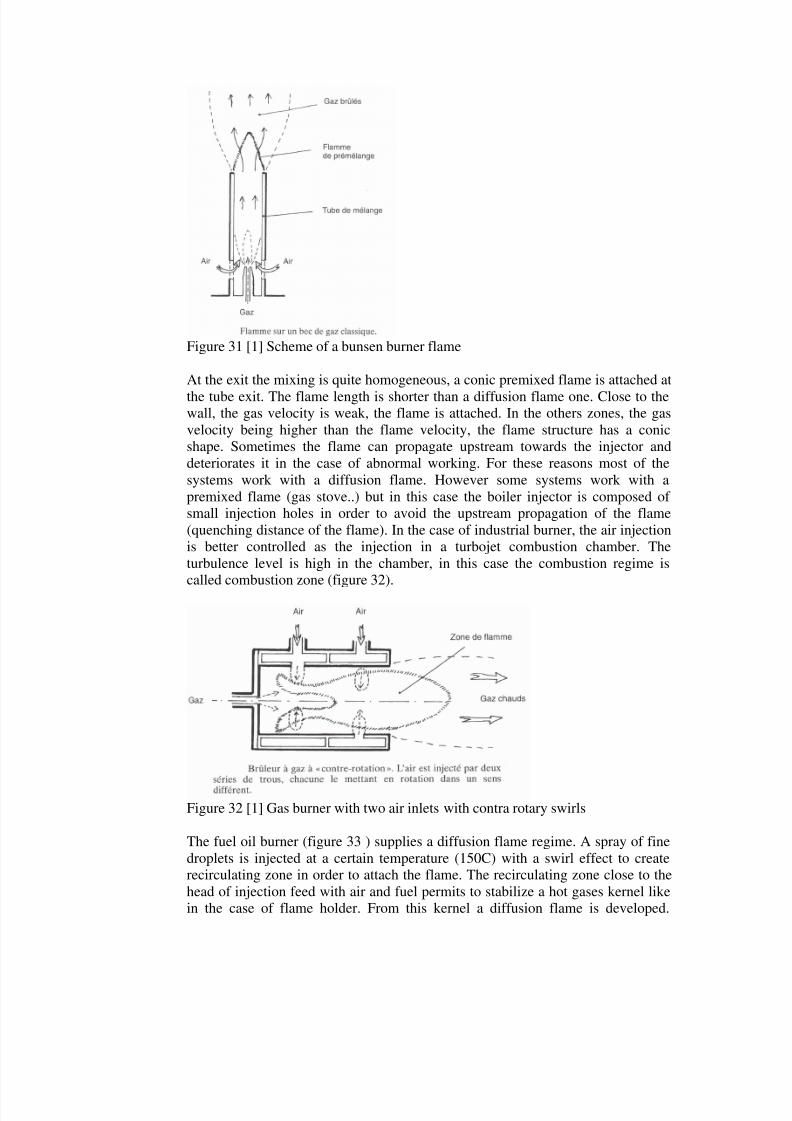
The burnersCurrent development of industrial or domestic furnaces, boiler…must be take intoaccount different criteria : efficiency, reduction of pollutant emissions and noise.We can distinguish gas boiler and the boiler using solid fuel (coal for example).The lighter is the simple boiler figure 30, the fuel is methane. The methane jetentrains a certain amount of airflow rate. After ignition we can see a diffusionflame as in candle case.
Figure 30 [1] Scheme of a lighter flame
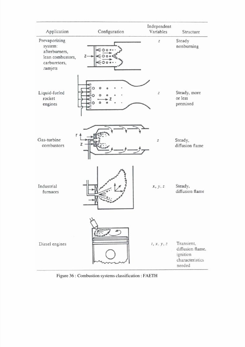
Bunsen burner used in laboratories generates a premixed flame. It is composed ofpremixing tube in which is located an injector surrounded by an air flux
8/10/2019 Two phase flow in combustion system
http://slidepdf.com/reader/full/two-phase-flow-in-combustion-system 25/177
Figure 31 [1] Scheme of a bunsen burner flame
At the exit the mixing is quite homogeneous, a conic premixed flame is attached at
the tube exit. The flame length is shorter than a diffusion flame one. Close to thewall, the gas velocity is weak, the flame is attached. In the others zones, the gasvelocity being higher than the flame velocity, the flame structure has a conicshape. Sometimes the flame can propagate upstream towards the injector anddeteriorates it in the case of abnormal working. For these reasons most of thesystems work with a diffusion flame. However some systems work with apremixed flame (gas stove..) but in this case the boiler injector is composed ofsmall injection holes in order to avoid the upstream propagation of the flame(quenching distance of the flame). In the case of industrial burner, the air injectionis better controlled as the injection in a turbojet combustion chamber. Theturbulence level is high in the chamber, in this case the combustion regime iscalled combustion zone (figure 32).
Figure 32 [1] Gas burner with two air inlets with contra rotary swirls
The fuel oil burner (figure 33 ) supplies a diffusion flame regime. A spray of finedroplets is injected at a certain temperature (150C) with a swirl effect to createrecirculating zone in order to attach the flame. The recirculating zone close to thehead of injection feed with air and fuel permits to stabilize a hot gases kernel likein the case of flame holder. From this kernel a diffusion flame is developed.

8/10/2019 Two phase flow in combustion system
http://slidepdf.com/reader/full/two-phase-flow-in-combustion-system 26/177
Overall air and fuel flow rate is injected upstream in the burner. The differentcombustion regimes are also in the case present at the droplet scale.
Figure 33 [1] Scheme of fuel oil burner in an industrial furnace
Fires
Combustion plays an important role in fire, explosion and detonation.
First consider an explosion creates by a leak of gas in a room, a spark can induce apremixed flame propagation which is called explosion. The first results came fromMallard et Le Chatelier works in the domain of firedamp explosion 1881.In stagnant air, the explosion induces pressure oscillations which can sometimescouple with the flame propagation to lead to a detonation propagating at highvelocity level (1000m/s). This phenomena has been studied for liquid or solidexplosives. The scramjet propulsion has also many common points with detonationpropagation (weak detonation). The vertical wall fire creates also a diffusion flamebetween air of the room and vapor coming from wall material(figure 34). Diffusionflame can be also observed on the sea surface resulting of a liquid sheetcombustion, in this case too, convection plays an important role(figure 35).
Figure 34 [1] Flame propagating close to an open polymer vertical wall

8/10/2019 Two phase flow in combustion system
http://slidepdf.com/reader/full/two-phase-flow-in-combustion-system 27/177
Figure 35 [1] Scheme of a flame above of liquid fluid reservoir
Forest fires. At high scale the fire can be seen as a premixed flame, but we canobserve a diffusion flame around each tree or around a tree package and also
isolated flame around a branch for example. In fact we can observe the samecombustion regime as in spray. Wind and turbulence have also an important effecton the flame shape (wake flame).
8/10/2019 Two phase flow in combustion system
http://slidepdf.com/reader/full/two-phase-flow-in-combustion-system 28/177
Refere
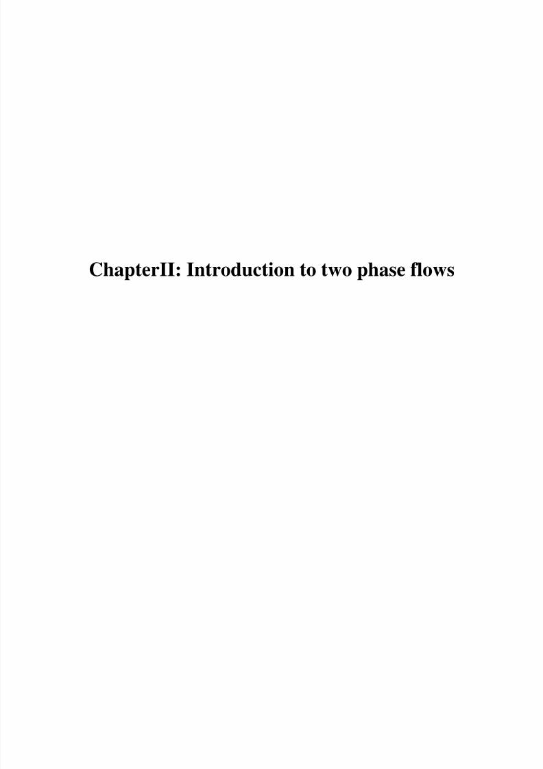
Figure 36 : Combustion systems classification : FAETH
8/10/2019 Two phase flow in combustion system
http://slidepdf.com/reader/full/two-phase-flow-in-combustion-system 29/177
ChapterII: Introduction to two phase flows

8/10/2019 Two phase flow in combustion system
http://slidepdf.com/reader/full/two-phase-flow-in-combustion-system 30/177
Multiphase Flows can be divided into four types:
- gas-liquid- gas-solid- liquid-solid- Liquid-solid-gas
Gas-liquid Bubbly flowsStratified flowsGas-droplets flows
Gas-solid gas-particles flowspneumatic TransportFluidizided beds
Liquid-solid Particles transport in a liquidHydraulic transportSediment Transport
Liquid-solid-gas Droplets-particles in a gaseous flow
Classification and multiphase flows examples
Many applications are concern by sprays, formation and droplet transport. The transformationof a liquid jet in spray involved many complex phenomena (primary and secondaryatomization, droplet turbulent dispersion, droplet evaporation, droplets collision, spray-wallinteraction ….. and has many industrial applications;
8/10/2019 Two phase flow in combustion system
http://slidepdf.com/reader/full/two-phase-flow-in-combustion-system 31/177
INDUSTRY
- Spray evaporation and combustion- Cooling by evaporation- Powder materials- Painting
- …….
AGRICULTURE-Culture treatment
ENVIRONNEMENT
- Humidification- Pollutant transport- Fire
MEDECINE
- Aerosols- …
GAZ EXPLORATION
- Two phase flows metering (Venturi measurement for example)
PROPULSION
- Gas turbine- Rocket motor- Diesel motor- Burner- Furnace
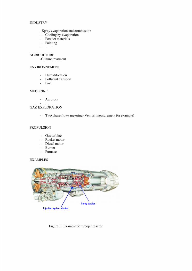
EXAMPLES
Injection system studies
Spray studies
Figure 1 : Example of turbojet reactor
8/10/2019 Two phase flow in combustion system
http://slidepdf.com/reader/full/two-phase-flow-in-combustion-system 32/177
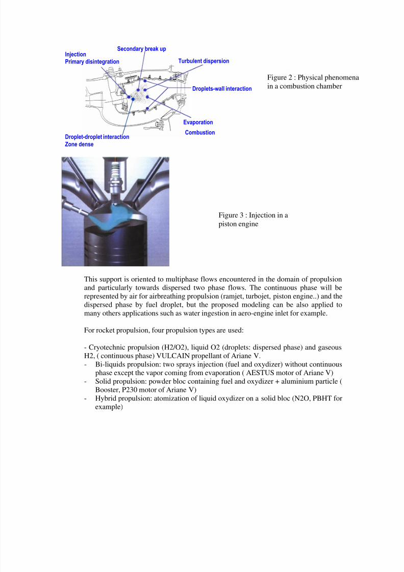
InjectionPrimary disintegration
Evaporation
CombustionDroplet-droplet interaction
Zone dense
Secondary break up
Turbulent dispersion
Droplets-wall interaction
This support is oriented to multiphase flows encountered in the domain of propulsionand particularly towards dispersed two phase flows. The continuous phase will berepresented by air for airbreathing propulsion (ramjet, turbojet, piston engine..) and thedispersed phase by fuel droplet, but the proposed modeling can be also applied tomany others applications such as water ingestion in aero-engine inlet for example.
For rocket propulsion, four propulsion types are used:
- Cryotechnic propulsion (H2/O2), liquid O2 (droplets: dispersed phase) and gaseousH2, ( continuous phase) VULCAIN propellant of Ariane V.- Bi-liquids propulsion: two sprays injection (fuel and oxydizer) without continuous
phase except the vapor coming from evaporation ( AESTUS motor of Ariane V)- Solid propulsion: powder bloc containing fuel and oxydizer + aluminium particle (
Booster, P230 motor of Ariane V)
- Hybrid propulsion: atomization of liquid oxydizer on a solid bloc (N2O, PBHT forexample)
Figure 2 : Physical phenomenain a combustion chamber
Figure 3 : Injection in apiston engine
8/10/2019 Two phase flow in combustion system
http://slidepdf.com/reader/full/two-phase-flow-in-combustion-system 33/177
8/10/2019 Two phase flow in combustion system
http://slidepdf.com/reader/full/two-phase-flow-in-combustion-system 34/177
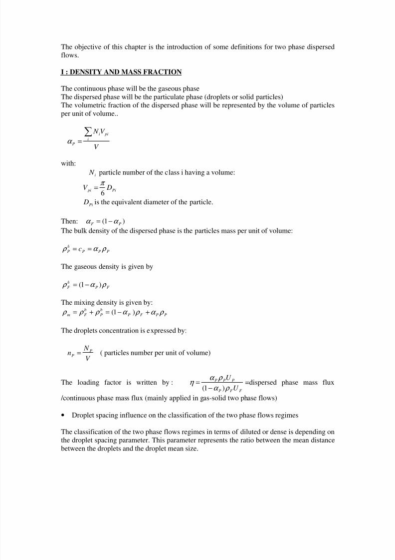
The objective of this chapter is the introduction of some definitions for two phase dispersedflows.
I : DENSITY AND MASS FRACTION
The continuous phase will be the gaseous phase
The dispersed phase will be the particulate phase (droplets or solid particles)The volumetric fraction of the dispersed phase will be represented by the volume of particlesper unit of volume..
V
V N i
pii
P
∑=α
with:
i N particle number of the class i having a volume:
Pi pi DV
6
π =
Pi D is the equivalent diameter of the particle.
Then: F α )1( Pα −= The bulk density of the dispersed phase is the particles mass per unit of volume:
PPP
b
P c ρ α ρ ==
The gaseous density is given by
F P
b
F ρ α ρ )1( −=
The mixing density is given by:
P
b
P
b
F m α ρ ρ ρ −=+= 1( PPF ρ α ρ +)
The droplets concentration is expressed by:
V
N n P
P = ( particles number per unit of volume)
The loading factor is written by :
F F P
PPP
U
U
ρ α
ρ α η
)1( −= =dispersed phase mass flux
/continuous phase mass flux (mainly applied in gas-solid two phase flows)
• Droplet spacing influence on the classification of the two phase flows regimes
The classification of the two phase flows regimes in terms of diluted or dense is depending onthe droplet spacing parameter. This parameter represents the ratio between the mean distancebetween the droplets and the droplet mean size.
8/10/2019 Two phase flow in combustion system
http://slidepdf.com/reader/full/two-phase-flow-in-combustion-system 35/177
For a cubic arrangement, the mean distance between the particles is given by:
3
1
)6
(PP
D
L
α
π = with
3
3
6 L
DP
π α =
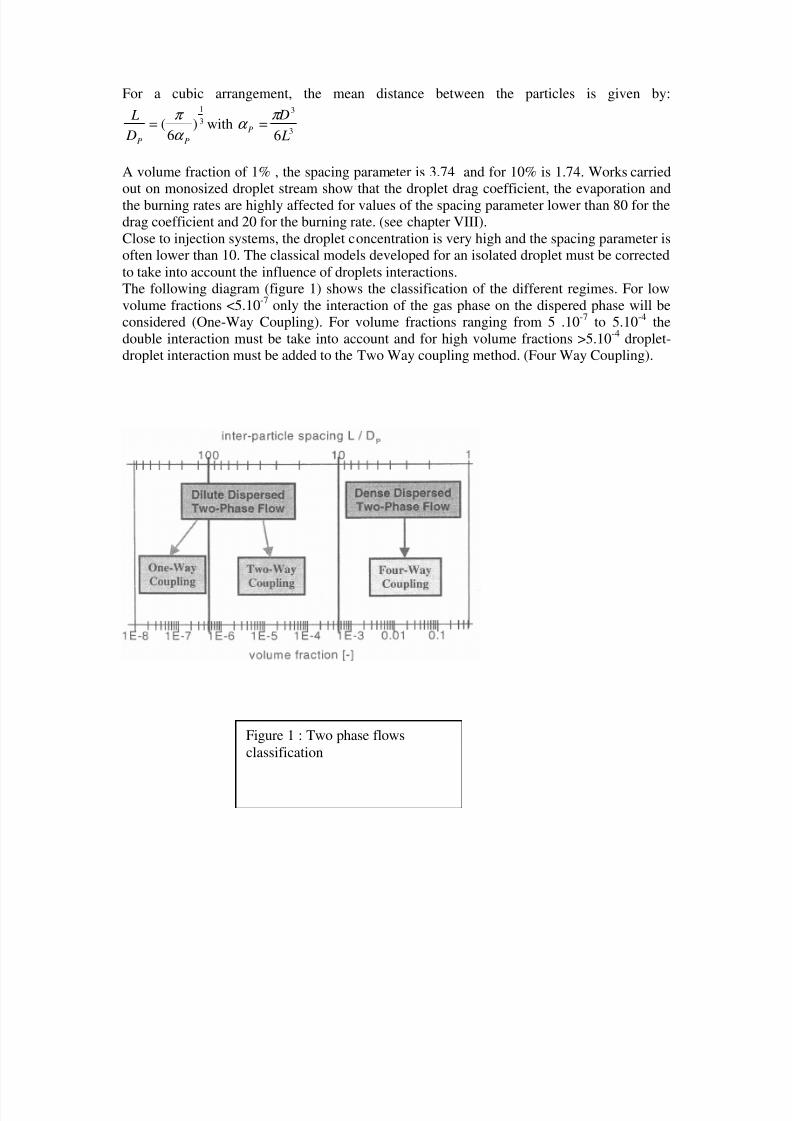
A volume fraction of 1% , the spacing parameter is 3.74 and for 10% is 1.74. Works carriedout on monosized droplet stream show that the droplet drag coefficient, the evaporation andthe burning rates are highly affected for values of the spacing parameter lower than 80 for thedrag coefficient and 20 for the burning rate. (see chapter VIII).Close to injection systems, the droplet concentration is very high and the spacing parameter isoften lower than 10. The classical models developed for an isolated droplet must be correctedto take into account the influence of droplets interactions.The following diagram (figure 1) shows the classification of the different regimes. For lowvolume fractions <5.10-7 only the interaction of the gas phase on the dispered phase will beconsidered (One-Way Coupling). For volume fractions ranging from 5 .10-7 to 5.10-4 thedouble interaction must be take into account and for high volume fractions >5.10 -4 droplet-droplet interaction must be added to the Two Way coupling method. (Four Way Coupling).
Figure 1 : Two phase flowsclassification
8/10/2019 Two phase flow in combustion system
http://slidepdf.com/reader/full/two-phase-flow-in-combustion-system 36/177
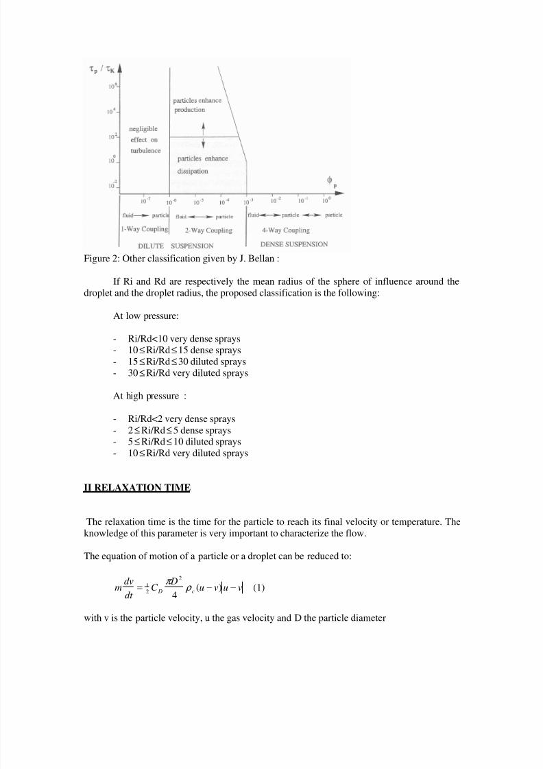
Figure 2: Other classification given by J. Bellan :
If Ri and Rd are respectively the mean radius of the sphere of influence around thedroplet and the droplet radius, the proposed classification is the following:
At low pressure:
- Ri/Rd<10 very dense sprays- 10 ≤ Ri/Rd ≤ 15 dense sprays- 15 ≤ Ri/Rd ≤ 30 diluted sprays- 30 ≤ Ri/Rd very diluted sprays
At high pressure :
- Ri/Rd<2 very dense sprays- 2 ≤ Ri/Rd≤ 5 dense sprays- 5 ≤ Ri/Rd≤ 10 diluted sprays- 10 ≤ Ri/Rd very diluted sprays
II RELAXATION TIME
The relaxation time is the time for the particle to reach its final velocity or temperature. Theknowledge of this parameter is very important to characterize the flow.
The equation of motion of a particle or a droplet can be reduced to:
vuvu D
C dt
dvm
c D −−= )(
4
2
21 ρ
π (1)
with v is the particle velocity, u the gas velocity and D the particle diameter
8/10/2019 Two phase flow in combustion system
http://slidepdf.com/reader/full/two-phase-flow-in-combustion-system 37/177
The particle Reynolds number is defined by: =ep R
c
c vu D
µ
ρ −
Dividing by the particle mass, the equation can be written by:
)(24
18 2 vu RC
Ddt dv eP D
P
c −= ρ
µ (2)
c µ is the viscosity of the continuous phase
For low Reynolds number ( eP R = 1, Stokes flow), the factor Cd=Rep/24
Dynamical relaxation time:
Introducing the “dynamic” relaxation time in the equation (2):
c
P
v
D
µ
ρ τ
18
2
=
Then the equation (2) can be written as: )(1
vudt
dv
v
−=τ
The solution of this equation, for a constant gas velocity u and for a droplet velocity v=0, is:
)1( v
t
euv τ
−
−=
vτ represents the time for a droplet to get 63% ( )1e
e− of the gaseous phase velocity.
This result is only valid for Stokes flows (Rep 1≅ ). For example for a water droplet of100 m µ size moving in air .30msv =τ
For higher Reynolds numbers:
c
P
v
D
µ
ρ τ
18
2
= f
1
with f=24
ep D Rc, DC corresponding in this case to the drag coefficient related to the Reynolds
number. (see chapter VI).
Thermal relaxation time:
The thermal balance equation of a particle can be written (neglecting the radiative flux):
)( Pcc
P
P T T D Nu
dt
dT mc −= πκ Nu is the Nusselt number, Pc the specific heat of the particle
and cK the thermal conductivity of the gaseous phase.

8/10/2019 Two phase flow in combustion system
http://slidepdf.com/reader/full/two-phase-flow-in-combustion-system 38/177
Dividing by Pcm. :
)(12
2 2 d c
PP
cP T T Dc
K Nu
dt
dT −=
ρ
For low Reynolds numbers, the ratio Nu/2 is close to 1. The other factor is thermal relaxationtime:
c
PP
T K
Dc
12
2 ρ τ =
Then :
)(1
d c
T
P T T dt
dT −=
τ
For the previous example (water droplet), the thermal relaxation time is T τ =145 ms.
Link between the two characteristic times :
Pr
1
3
2
3
2
3
212
18 2
2
P
c
Pcd
c
PP
cP
T
v
c
c
cc
K
c
K
Dc
K D====
µ µ ρ µ
ρ
τ
τ with Pr the Prandtl number and c
C the
specific heat at constant pressure.
Stokes number
The Stokes number is defined by:
F
v
vSt τ
τ
= where F τ is the characteristic time of the gaseous phase. For turbulent flow the characteristictime will be the temporal integral scale of the turbulence. For a periodic unsteady flow(coherent structures) this time will be represented by the period of the vortices. For a Venturiflow for example, the characteristic time will be represented by the ratio between the diameterof the Venturi and the flow velocity.
If vSt <<1 The particle relaxation time is very low and the droplet velocity will be very close
to the gaseous phase.
Ifv
St >>1 The particles are not affected by the gaseous phase.
If vSt 1≅ In the case of unsteady flow, the particles will be located at the periphery of the
vortices (mixing layer configuration for example), some of them will be centrifuged. In thiscase the expansion will be maximum.
8/10/2019 Two phase flow in combustion system
http://slidepdf.com/reader/full/two-phase-flow-in-combustion-system 39/177
III. DILUTED AND DENSE TWO PHASE FLOWS
A two phase flow is considered as a diluted flow if the motion of the particles is controlled bythe fluid forces (drag and lift forces).
That is quantified by :c
v
τ
τ 1< where cτ is the mean collision time between particles.
If :c
v
τ
τ >1 The particle has not enough time to respond to the fluid forces before the next
collision. In this case the flow is dense.
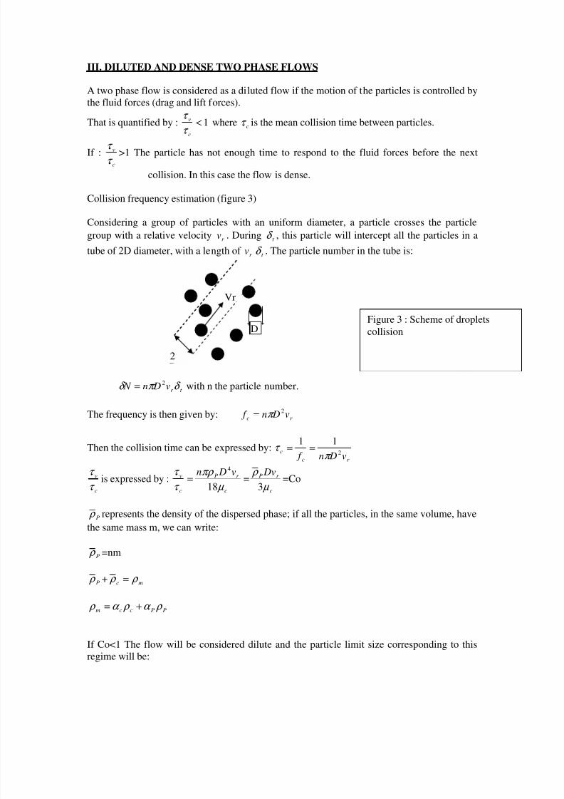
Collision frequency estimation (figure 3)
Considering a group of particles with an uniform diameter, a particle crosses the particlegroup with a relative velocity r v . During t δ , this particle will intercept all the particles in a
tube of 2D diameter, with a length of r v t δ . The particle number in the tube is:
t r v Dn N δ π δ 2= with n the particle number.
The frequency is then given by:r c
v Dn f 2π =
Then the collision time can be expressed by:r c
cv Dn f 2
11
π τ ==
c
v
τ
τ is expressed by :
c
v
τ
τ
c
r P v Dn
µ
πρ
18
4
= =c
r P Dv
µ
ρ
3=Co
P ρ represents the density of the dispersed phase; if all the particles, in the same volume, havethe same mass m, we can write:
P ρ =nm
P ρ + mc ρ ρ =
PPccm ρ α ρ α ρ +=
If Co<1 The flow will be considered dilute and the particle limit size corresponding to thisregime will be:
2
Vr
DFigure 3 : Scheme of dropletscollision
8/10/2019 Two phase flow in combustion system
http://slidepdf.com/reader/full/two-phase-flow-in-combustion-system 40/177
r P
c
v D
ρ
µ 3<
r c
c
v Z D
ρ
µ 3< with
c
d
M
M Z = mass flow rates ratio between the dispersed phase and the gaseous
phase.
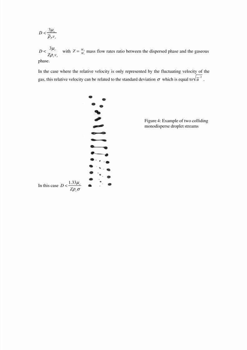
In the case where the relative velocity is only represented by the fluctuating velocity of the
gas, this relative velocity can be related to the standard deviation σ which is equal to2'
u .
In this caseσ ρ µ c
c
Z D 33.1<
Figure 4: Example of two collidingmonodisperse droplet streams
8/10/2019 Two phase flow in combustion system
http://slidepdf.com/reader/full/two-phase-flow-in-combustion-system 41/177
Chapter IV: Different approaches for twophase flows numerical simulation
8/10/2019 Two phase flow in combustion system
http://slidepdf.com/reader/full/two-phase-flow-in-combustion-system 42/177
I. GASEOUS PHASE NUMERICAL SIMULATION :
I.1 Introduction
The statistic modeling of a turbulent flow, based on RANS (Reynolds Average Navier Stokesequations) is devoted to turbulent flows statistically steady or to the flows where the time
evolution of the physical properties is very low. With this statistic approach, all the scales ofthe turbulence are modeled, but the models used are not universal and they are adjusted withsome constants. However the statistic approach permits to simulation complex configurationsbecause the mean values do not need very precise spatial and temporal discretization incomparison with unsteady flow field presenting high gradients. In parallel some deterministicapproaches are now used. The Direct Numerical Simulation consists in solving all the spatialand temporal scales of the turbulence from the energetic largest one to the dissipative scales(Kolmogorov scale). This approach is not yet used to simulate very complex geometries suchas a combustion chamber of a turbojet. An intermediate approach which is now more andmore used is the LES technique (Large Eddy Simulation). In this approach, the largest scales(the more energetic one) are computed and the smaller one are modeled (Sub Grid Model).This technique is well adapted for the simulation of reacting two phase flows in combustion
chambers. The presence of jets, mixing layers, recirculation zones induces the formation oflarge vortices piloting the fuel-air mixing an the turbulent transfers.
I.2 Scales and main characteristics of the turbulence
Turbulence intensity :
u’ ),( t x j , v’ ),( t x j , w’ ),( t x j are the fluctuating velocities
The following quantity is called turbulence intensity :
U
u I u
2'= for 1D flow
222
2'2'2'
W V U
wvu I e
++
++= for 3D flow
whereU is the mean value of the component in x direction of the velocity vector
Micro and macro Taylor scales :
The one point correlation function is defined by :
2'2'
''
'
vu
vu R
vu =

8/10/2019 Two phase flow in combustion system
http://slidepdf.com/reader/full/two-phase-flow-in-combustion-system 43/177
For Ctet t t === 0' , respectively '
x x = Cte x == 0 , this definition leads to the temporalrespectively spatial auto-correlation function. For homogeneous turbulent fields and forunsteady state, these functions are written :
1),(.),(
),(),(),(
02'
02'
0'
0'
0
≤+
+=
t r xut xu
t r xut xut r R or 1
),(.),(
),(),(),(
02'
02'
0'
0'
0 ≤+
∆+=
t r xut xu
t t xut xut x R
R
1
0 r ou τ
The macro temporal and spatial Taylor scales are written :
∫∞
=Λ0
),()( τ d t r Rt and ∫∞
=Λ0
),()( dr r Rr τ
These values give an order of time or distance step where the fluctuating velocity ),(' t xu is
itself correlated
The micro-scales (temporal and spatial) are defined by :
)(
2)
),((
202
2
t r
t r Rr
λ −=
∂
∂= and
)(
2)
),((
202
2
r
r R
λ τ
τ
τ −=
∂
∂=
These micro-scales provided us an estimation of the amount of dissipation, they do notrepresent scales of vortices.Now we will introduce the Kolgomorov scales characterising the dissipation of the structure.
Kolgomorov scales
We associate to the smallest scales of the flow the different scales respectively: the length
( )η , and the velocityτ
η =v
These smallest scales correspond to a balance between the inertial and viscosity forces:
1≈υ
η v (Reynolds number)

8/10/2019 Two phase flow in combustion system
http://slidepdf.com/reader/full/two-phase-flow-in-combustion-system 44/177
Following Kolgomorov : 2
1
)( −
≈υ
ε τ ε is the dissipation rate such as :
2
2'
30λ
υ ε u
=
in the case of isotropic and homogeneous turbulence
Then we can deduced the two scales of kolgomorov (the smallest scales in the flow),depending of the dissipation rate and the viscosityε , υ
4
1
)(3
ε
υ η == k l et 4
1
).( ε υ =v
Kinetic energy of turbulence
)''(2
1 22'2wvuk ++=
Spectrum of the length scales of the turbulence
The kinetic energy of the turbulence is distributed on different wave numbers from 0 to ∞
∫∞
=0
)( dnn E k , n : wave number
Ln(t kl
n E )()
5
Slope =5/33
Ln(nlt)Figure 1: Kolgomorov spectrum
Lt : spatial integral scale of the turbulence = r Λ
2
1'
k
lt
L α τ = = temporal integral scale of the turbulence = t
Λ , where cte='α

8/10/2019 Two phase flow in combustion system
http://slidepdf.com/reader/full/two-phase-flow-in-combustion-system 45/177
E(K) RANS (modeling)
DNS
LES computation LES modeling
Kc K
Figure 2: Different approaches for flow computation
U DNS LES
RANS
t
Figure 3: Example of flow velocity computations from different approaches.
8/10/2019 Two phase flow in combustion system
http://slidepdf.com/reader/full/two-phase-flow-in-combustion-system 46/177
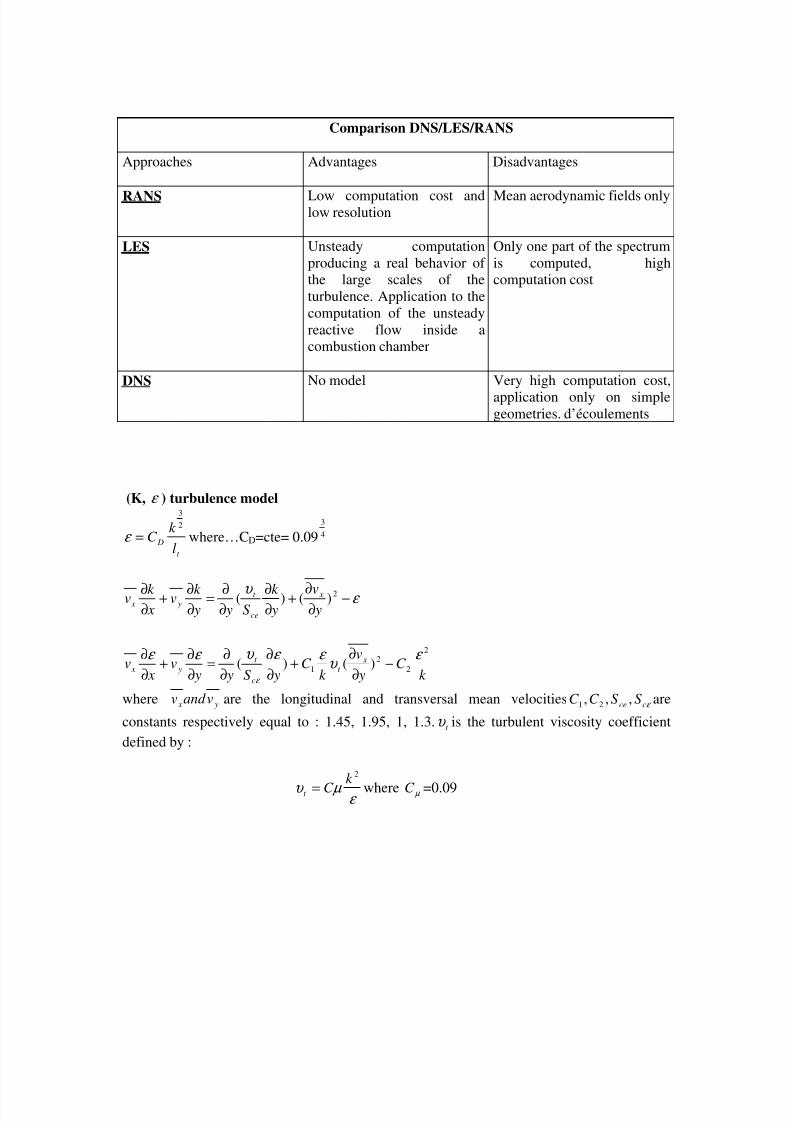
Comparison DNS/LES/RANS
Approaches Advantages Disadvantages
RANS Low computation cost andlow resolution Mean aerodynamic fields only
LES Unsteady computationproducing a real behavior ofthe large scales of theturbulence. Application to thecomputation of the unsteadyreactive flow inside acombustion chamber
Only one part of the spectrumis computed, highcomputation cost
DNS No model Very high computation cost,
application only on simplegeometries. d’écoulements
(K, ε ) turbulence model
t
Dl
k C
2
3
=ε where…CD=cte= 0.09 4
3
ε υ −∂∂+
∂∂
∂∂=
∂∂+
∂∂ 2)()(
yv
yk
S y yk v
xk v x
ce
t y x
k C
y
v
k C
yS y yv
xv x
t
c
t y x
2
22
1 )()( ε υ
ε ε υ ε ε
ε
−∂
∂+
∂
∂
∂
∂=
∂
∂+
∂
∂
where y x vand v are the longitudinal and transversal mean velocities ε cce
S S C C ,,, 21 are
constants respectively equal to : 1.45, 1.95, 1, 1.3. t υ is the turbulent viscosity coefficient
defined by :
ε µ υ
2
k C t = where µ C =0.09

8/10/2019 Two phase flow in combustion system
http://slidepdf.com/reader/full/two-phase-flow-in-combustion-system 47/177
47
II. TWO APPROACHES FOR TWO PHASE FLOW MODELING
- Euler (continuous phase), Euler for the dispersed phase
- Euler (continuous phase), Lagrange for the dispersed phase
The first approach will be presented very briefly, the second will be improved in the frame ofthese lectures.
II.1 Euler/Euler approach
Two methods are distinguished: deterministic and statistics
Deterministic eulerian approach (dilute flow or two fluid model):
- hypothesis:- H1 – the particle phase is treated as a continuous field
- H2 – the volume of the particles is negligible and the Stokes number computedon the collision characteristic time is lower than1.
- H3 – the gas specific heat is constant, the gas is considered perfect andchemically frozen.
- H4 – the particle specific heat is constant, and there is no temperature gradientinside the particles.
- H5 – the particles are spherical with no roughness- H6 – the density of tha particle is very higher than the gas one- H7 – the Brownian motion of the particles is negligible.- H8 – the trajectory of the particle is computed using a deterministic method.
With these hypothesis, it is possible to identify the mass concentration of gas and its density..Considering m classes of particles, the equations of conservation of gas can be written:
∑=
=+∂
∂ m
j
j jP N udivt 1
,)()( ω ρ ρ &r
−=−⊗+∂
∂∑
=
m
j
jP j jP u N uudivu
t 1,,)(
r&
rrrω σ ρ ρ j
m
j
jP F N
r
∑=1
,
j
m
j
jP
m
j
jP j jP
m
j
jP
jP jP
j jP Q N uF N h
uu N quu E div E
t ∑∑∑
===
−−
+=+−+∂
∂
1,
1,,
1,
,,, 2
..)(
rrrr
&rrr
ω σ ρ ρ
jF
r : gas force on a particle of class j (mainly the drag force)
jQ : heat transfer from the gas to a particle of class j (convection heat)
jω & : mass transfer between gas and particle of class j (evaporation, condensation..)
To these equations, a turbulence model must be added. The more used is a twoequations model ε ,K , respectively the turbulent kinetic energy and the viscous dissipation ofthe turbulent kinetic energy (Jones et Launder)
8/10/2019 Two phase flow in combustion system
http://slidepdf.com/reader/full/two-phase-flow-in-combustion-system 48/177
48
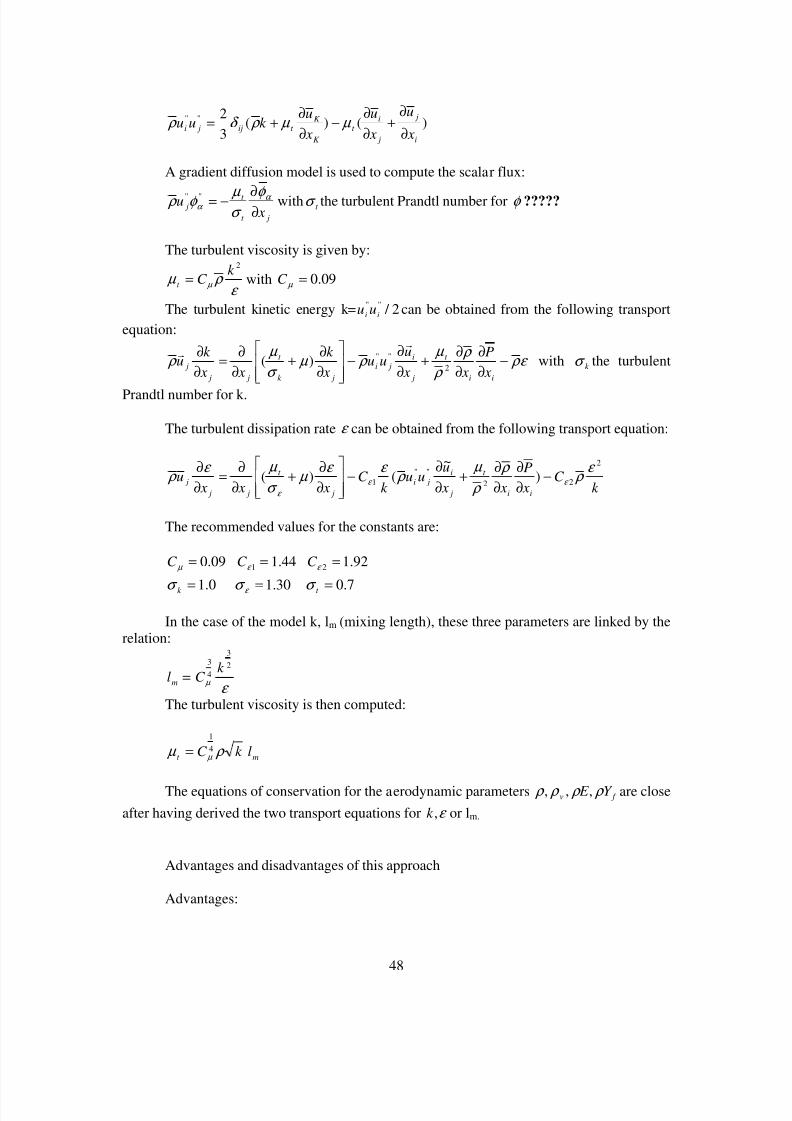
)()(3
2""
i
j
j
i
t
K
K t ij ji
x
u
x
u
x
uk uu
∂
∂+
∂
∂−
∂
∂+= µ µ ρ δ ρ
A gradient diffusion model is used to compute the scalar flux:
jt
t j
xu
∂∂−= α
α φ σ µ φ ρ "" with t σ the turbulent Prandtl number for φ ?????
The turbulent viscosity is given by:
ε ρ µ µ
2k
C t = with 09.0= µ C
The turbulent kinetic energy k= 2 / ""ii
uu can be obtained from the following transportequation:
ε ρ ρ
ρ
µ ρ µ
σ
µ ρ −
∂
∂
∂
∂+
∂
∂−
∂
∂+
∂
∂=
∂
∂
ii
t
j
i ji
jk
t
j j
j x
P
x x
uuu
x
k
x x
k u
2"")(
rr
with k σ the turbulent
Prandtl number for k.
The turbulent dissipation rate ε can be obtained from the following transport equation:
k C
x
P
x x
uuu
k C
x x xu
ii
t
j
i
ji
j
t
j j
j
2
22""
1 )~
()( ε
ρ ρ
ρ
µ ρ
ε ε µ
σ
µ ε ρ ε ε
ε
−∂
∂
∂
∂+
∂
∂−
∂
∂+
∂
∂=
∂
∂
The recommended values for the constants are:
09.0= µ C 44.11 =ε C 92.12 =ε C
0.1=k σ 30.1=ε σ 7.0=t σ
In the case of the model k, lm (mixing length), these three parameters are linked by therelation:
ε µ
2
3
4
3k
C lm =
The turbulent viscosity is then computed:
k C t
ρ µ µ 4
1
=m
l
The equations of conservation for the aerodynamic parameters f v Y E ρ ρ ρ ρ ,,, are closeafter having derived the two transport equations for ε ,k or lm.
Advantages and disadvantages of this approach
Advantages:
8/10/2019 Two phase flow in combustion system
http://slidepdf.com/reader/full/two-phase-flow-in-combustion-system 49/177
49
- Easy elaboration of the code, the computations for the two phases are identical- The volume occupied by the dispersed phase is taken into account in the equations.- The action of the dispersed phase on the gas phase . (Two Way Coupling) is
“naturally” taken into account.
Disadvantages:
- The integration of the physical models due to the presence of the dispersed phaseis very difficult: droplet evaporation, condensation, atomisation, droplet-wallinteraction, secondary break up, collision….
- Difficulties to considered a polydisperse size distribution for the dispersed phase,that is a main disadvantage for this method, in different burners at the exit ofinjection devices the spray is polydisperse.
- The cost can become high by considering a polydisperse size distribution.
- Conclusion : The Euler approach is mainly devoted to treat dense two phase flowsin non reactive regime and for a low droplet size dispersion.
Some researches are now lead to couple the two approaches (Euler-Euler and Euler-
Lagrange) to solve very complex flows presenting dense and dilute zones.
II.2 Euler/Lagrange approach
The continuous gaseous phase is always computed with an eulerian approach (samemethod), except the coupling between the two phases. The chapter IX will be devoted to thisapproach.
Lagrangian approach for the dispersed phase:
- Simplified approach (limited to a steady computation): Individual trajectory iscomputed and each particle represents a certain percentage of the total mass of thedispersed phase.
- General approach (valid for steady and unsteady flows): particles or droplets areconsidered as packages. These packages are injected simultaneously or withdifferent injection frequencies. The particles velocity and temperature in thepackage have the same value as an individual droplet.
On For droplet trajectories computation, two methods can be used: the deterministicapproach (no effect of the turbulence on the droplet trajectory)and the stochasticapproach (influence of the turbulence on the droplet dispersion).- The coupling with the continuous phase can be done for each time step or for sometime step depending of the application and the importance of source terms bycomputing and introducing the source terms in the equations of conservation.
Advantages and disadvantages:
Advantages
- The using is very simple (some problems can be encountered for the Two Waycoupling depending of the importance of sources terms.

8/10/2019 Two phase flow in combustion system
http://slidepdf.com/reader/full/two-phase-flow-in-combustion-system 50/177
50
- The integration of the physical models is very easy, it is for this reason that thisapproach is often used to simulate the reactive two phase flows inside acombustion chamber of air-breathing or rocket engines
- Different injection points can be chosen with for each point different size classes(example : to compute a spray, 10 injection points are generally chosen with 5 sizeper point, each class representing a droplet package. Each package can be
injectedwith the one frequency. The droplet size, velocity, temperature andfrequency are provided by experiment by using optical techniques such as:Malvern, PDPA (for the droplet size and velocity), LDA (for the aerodynamicfield), rainbow and LIF (for the droplet temperature)…
Disadvantages:
- The computation cost can become highThe volume occupied by the particles is not taken into account, inducing someproblems for dense two flow computations. However, to consider a four waycoupling some empirical correlation can be used to treat the droplet-dropletinteractions. Some correlation have been derived by ONERA to correct the
evolution of the drag coefficient, the evaporation rate and the burning rates with thedroplet spacing (ratio between the mean distance between the drplets and the meansize of the droplets.
Figure 4 : Droplets evaporation in a backward facing stepconfi uration
8/10/2019 Two phase flow in combustion system
http://slidepdf.com/reader/full/two-phase-flow-in-combustion-system 51/177
51
Chapter V: Spray formation
8/10/2019 Two phase flow in combustion system
http://slidepdf.com/reader/full/two-phase-flow-in-combustion-system 52/177
52
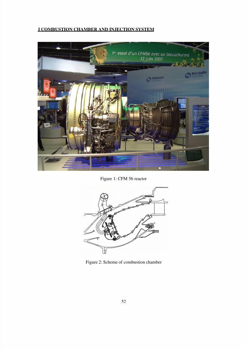
I COMBUSTION CHAMBER AND INJECTION SYSTEM
Figure 1: CFM 56 reactor
Figure 2: Scheme of combustion chamber

8/10/2019 Two phase flow in combustion system
http://slidepdf.com/reader/full/two-phase-flow-in-combustion-system 53/177
53
Figure 3: Main combustion phenomena
Figure 4: View of one sector of the combustion chamber

8/10/2019 Two phase flow in combustion system
http://slidepdf.com/reader/full/two-phase-flow-in-combustion-system 54/177
54
Monosized injector for research
Piezoelectric
V
30µm< Dg
2 < C = Sg / Dg < 7
OrificeDisk
Liqui
+-
~
Thermocoupl
Turbo et Airblast
Fue
Ai
Pressure
Fue
Rocket
Oxidiser
Hypergol
Fuel
Cryogenic
Gas H2
Liquid
8/10/2019 Two phase flow in combustion system
http://slidepdf.com/reader/full/two-phase-flow-in-combustion-system 55/177
55
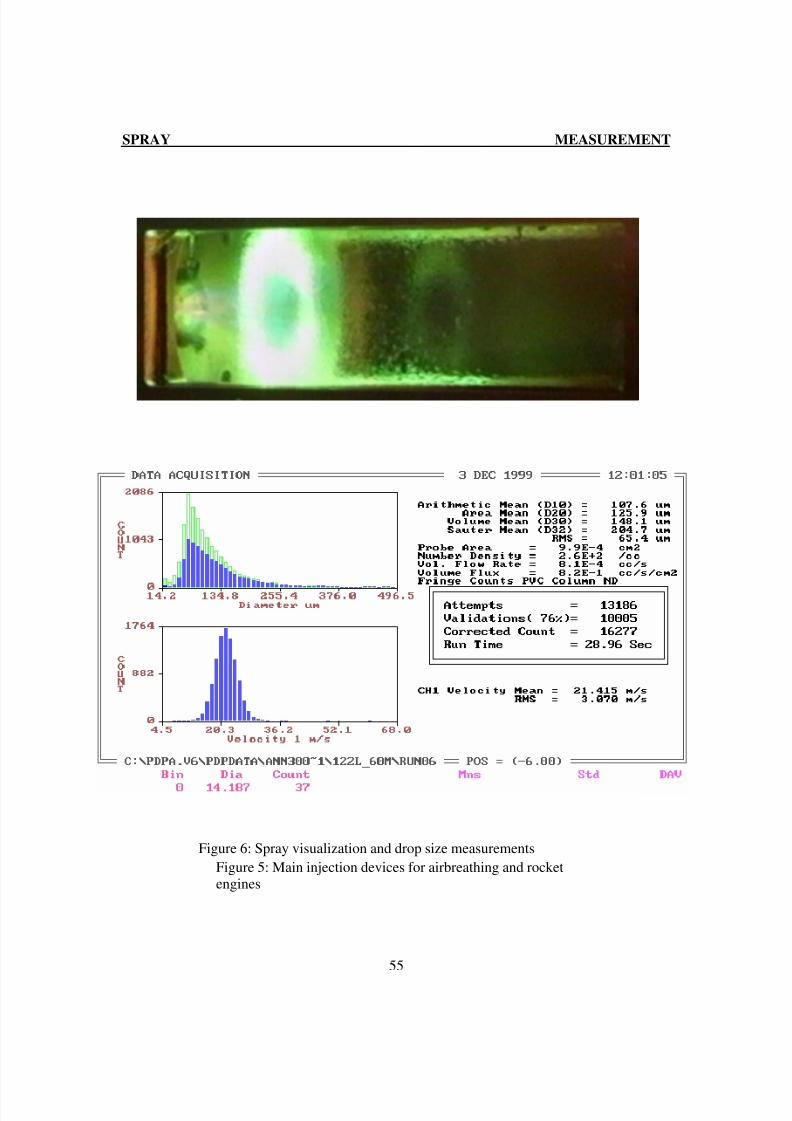
SPRAY MEASUREMENT
Figure 5: Main injection devices for airbreathing and rocketengines
Figure 6: Spray visualization and drop size measurements

8/10/2019 Two phase flow in combustion system
http://slidepdf.com/reader/full/two-phase-flow-in-combustion-system 56/177
56
II PRIMARY AND SECONDARY LIQUID SHEET BEAK UPAtomisationThe initial conditions for the dispersed phase in the most hard problem to be solved in two
phase flows modelling. Some injection devices are shown on the figure 5. Atomisation regimeis not yet well known and usually the droplet characteristics (size, velocity and fuel mass flow
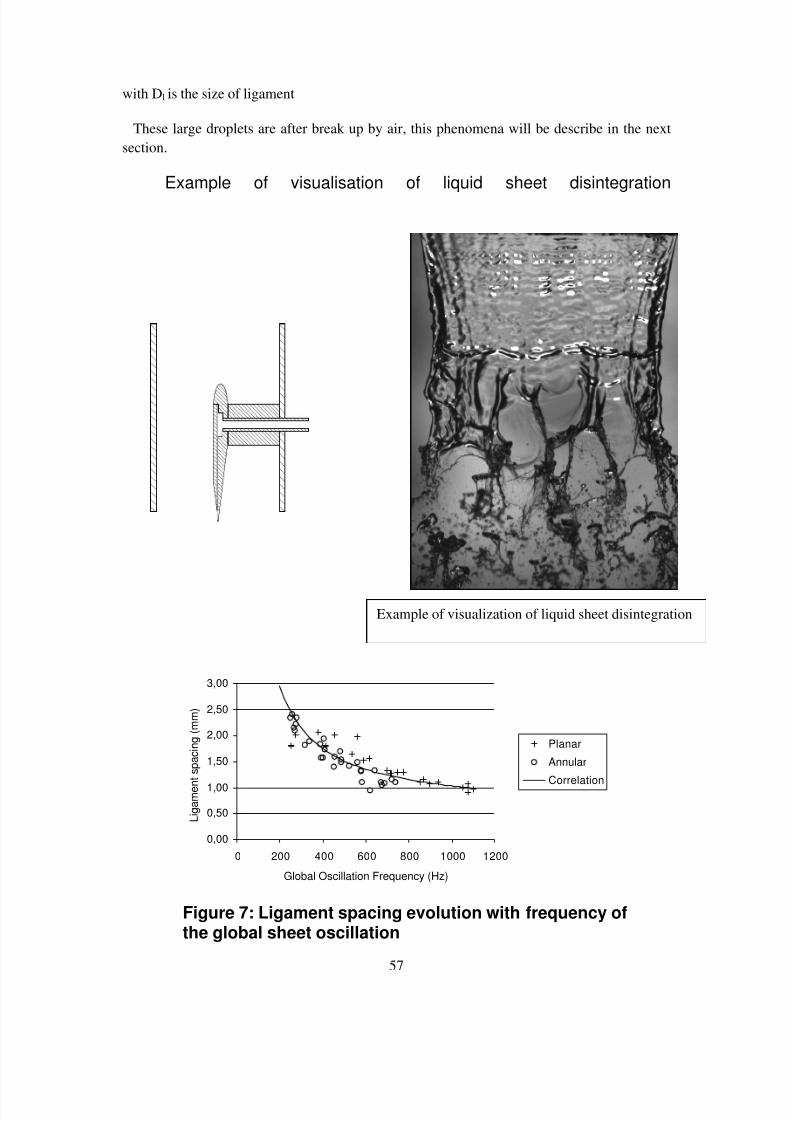
rate) close to the injection point are coming from measurements by mean PDPA, MALVERNtechniques (figure 6).However, Some researches are developed in the domain of atomisation. As example [3] wewill present an approach to improve the knowledge of liquid sheet disintegration byaerodynamic forces (airblast atomizer).A basic experiment was designed to study the break up of a planar liquid sheet induced by ahigh velocity air stream. A liquid sheet is generated from the central duct with a speed up to 9m/s (figure 7). The liquid of simulation is water. The liquid film is 300 µm thickness and 18mm width. The injector is located at the exit of the air duct. The flow velocity can be greaterthan 100m/s. This experiment allows a parametric study about the evolution of the break upwith air velocity, liquid velocity, the turbulence level (air and air), liquid sheet thickness andliquid properties by adding tracers to modify the surface tension and the viscosity.
Visualisations of the disintegration is carried out by using Video camera and stroboscopicback lighting technique ([4], figure 7). Longitudinal waves ( called primary instability) appearfirst on the planar sheet by a primary instability mechanism. After these waves are perturbedand become unstable and produce the 3D waves. This phenomena is called the secondaryinstability. Actually we think that these 3D waves are produced not by the primary instabilitybut by the instabilities generated by the two co-flowing air streams. From these Waves areproduced ligaments which then give large droplets and after small droplets by dropletsecondary break up.The characteristics of the droplets produced far from the exit of the injector are extremelydependant of wavelength of the secondary oscillation. The wavelength of the instability isprovided by a post processing of the images recorded.The expression obtained is the following :
M f 1.0* =
Where * f lu
t f = is the non dimensional frequency, M is the momentum ratio of the two
fluxes, t the liquid sheet thickness, U l the liquid velocity and f the frequency of the global
oscillation of the sheet.The wavelength of the secondary oscillation [5] is expressed by a direct relation of thefrequency of the global oscillation of the waves (figure 7).
+= 548.0)(sec mmλ )(
5.479
Hz f g
Recent works on annular liquid sheet (figure 7 ) give the same results as planar sheet if theratio between the liquid sheet thickness ant the curvature radius is small.The next step is the break up of the ligaments in large droplets. Rayleigh theory is often usedto compute the droplet size :
Dp = 1.9 Dl
8/10/2019 Two phase flow in combustion system
http://slidepdf.com/reader/full/two-phase-flow-in-combustion-system 57/177

8/10/2019 Two phase flow in combustion system
http://slidepdf.com/reader/full/two-phase-flow-in-combustion-system 58/177
8/10/2019 Two phase flow in combustion system
http://slidepdf.com/reader/full/two-phase-flow-in-combustion-system 59/177
59
For numerical purposes, the exponential law has to be discretised [7].This current model gives results in a good agreement with experimental results (figure 10).Others models of primary and secondary break up will be proposed in one
exrercise.
References:
[1] FAETH, G.M, current status of droplet and liquid combustion.Progress. Energy Comb. Sciences, Vol3, pp191-224, 1997
[2] BORGHI, R, LOISON, S, 24th Symp (Int) on combustion, pp 1541-1547, 1992.
[3] CARENTZ,H, Etude de la désintégration d’une nappe liquide mincePHD Thesis, April 2000, university Paris VI.
[4] BERTHOUMIEU, P, CARENTZ, H, LAVERGNE, G Study of planar liquid sheetdisintegration.
ILASS 97
[5] BERTHOUMIEU, P, CARENTZ. Experimental Study of a Thin Planar Liquid SheetDisintegration.Paper submitted to ICLASS 2000.
[6] PILCH, M, ERDMANN, C, A, Use of break-up time data and velocity history data topredict the maximum size of stable fragments for acceleration induced break-up of liquid dropInt Journal Multiphase Flow 13 (6), pp741-757
[7] BERTHOUMIEU, P, CARENTZ, H, LAVERGNE, G, VILLEDIEU P Contribution todroplet break-up analysis
Int Journal of Heat and Fluid Flow 20(1999), pp 492-498
8/10/2019 Two phase flow in combustion system
http://slidepdf.com/reader/full/two-phase-flow-in-combustion-system 60/177
60
Figure 5
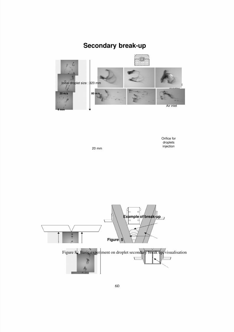
Secondary break-up
A
Orifice fordropletsinjection
Air inlet
Monosizedinjector
4 mm
20 m/s 80 m/s
20 mm
Initial droplet size : 320 mm
Example of break-up
Figure 8 : Basic experiment on droplet secondary break up, visualisation

8/10/2019 Two phase flow in combustion system
http://slidepdf.com/reader/full/two-phase-flow-in-combustion-system 61/177
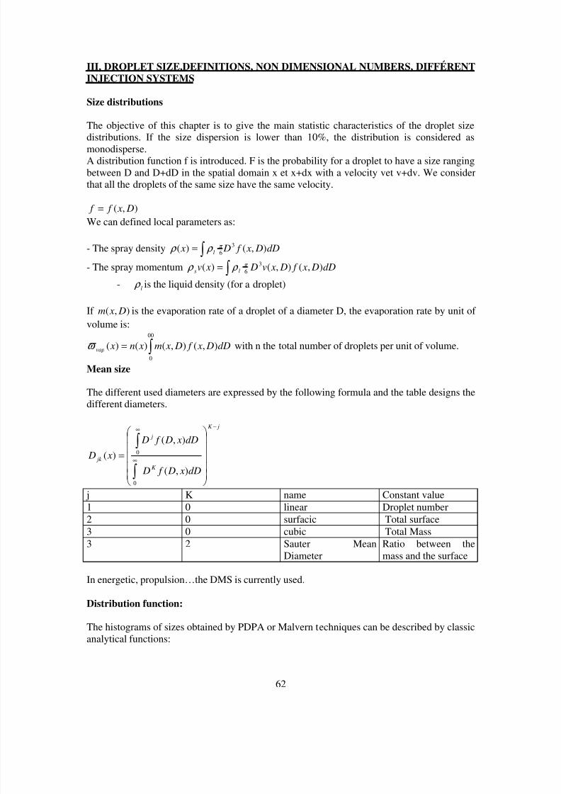
8/10/2019 Two phase flow in combustion system
http://slidepdf.com/reader/full/two-phase-flow-in-combustion-system 62/177

8/10/2019 Two phase flow in combustion system
http://slidepdf.com/reader/full/two-phase-flow-in-combustion-system 63/177
63
- Normal law2)(log)( D
D e D f β α −=
- Rosin Ramler law De D D f β γ α −−= 1)(
- Nukiyama Tanasawa law:γ β α De D D f −= 5)(
γ β α ,, are constants evaluated from experiments.
8/10/2019 Two phase flow in combustion system
http://slidepdf.com/reader/full/two-phase-flow-in-combustion-system 64/177
64
Chapter VI: Turbulent dispersion of theliquid phase

8/10/2019 Two phase flow in combustion system
http://slidepdf.com/reader/full/two-phase-flow-in-combustion-system 65/177
65
I. DRAG COEFFICIENT OF A SPHERICAL PARTICLE (OR DROPLET)
Equation of motion of a particle in a gaseous field: Odar and Hamilton equation:
Main hypothesis:
- Droplets are inert, spherical- No rotation of the droplets- The droplet density is very higher than the gas one.
gV V V V D
C
dt
V d PgPg
PP
d gP rrrrrr
+−−= )(4
3
ρ
ρ (I) P
P V dt
X d rr
=
PV
r
et gV
r
respectively the instantaneous velocities of the particle andthe gas
P ρ et g
ρ respectively the densities of the particle and the gas
=d C drag coefficient of the particle (or the droplet)
=P D particle diameter (or the droplet)
g
PgPg
P
DV V Re
µ
ρ rr
−= Reynolds number
In the case of a numerical simulation, at each time step, the values ofthe previous parameters must be known. Others equations for evaporation andcombustion must be introduced and solve simultaneously.
PP
Pd D
Kn D
LC M Re f C λ
=== ,,,(
With M : Mach number, C : spacing parameter, Kn : Knudsen number
For incompressible subsonic dilute flows
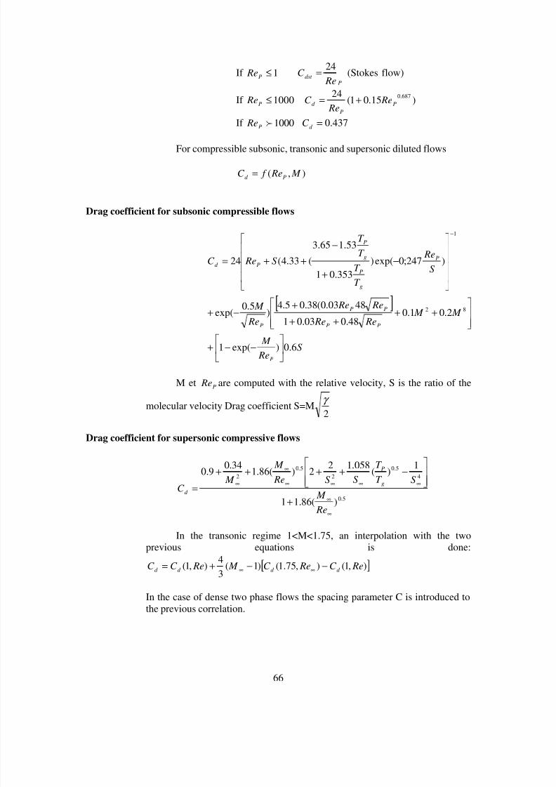
8/10/2019 Two phase flow in combustion system
http://slidepdf.com/reader/full/two-phase-flow-in-combustion-system 66/177
66
If 1≤P Re P
dst Re
C 24
= (Stokes flow)
If 1000≤P Re )15.01(24 687.0
P
P
d Re Re
C +=
If 1000fP Re 437.0=d
C
For compressible subsonic, transonic and supersonic diluted flows
),( M Re f C Pd
=
Drag coefficient for subsonic compressible flows
[ ]
S Re
M
M M Re Re
Re Re
Re
M
S
Re
T
T
T
T
S ReC
P
PP
PP
P
P
g
P
g
P
Pd
6.0)exp(1
2.01.048.003.01
4803.0(38.05.4)
5.0exp(
)247;0exp()
353.01
53.165.3
(33.4(24
82
1
−−+
++
++
+−+
−
+
−
++=
−
M et P Re are computed with the relative velocity, S is the ratio of the
molecular velocity Drag coefficient S=M2
γ
Drag coefficient for supersonic compressive flows
5.0
45.0
25.0
2
)(86.11
1)(
058.122)(86.1
34.09.0
∞
∞
∞∞∞∞
∞
∞
+
−++++
=
Re
M
S T
T
S S Re
M
M C
g
P
d
In the transonic regime 1<M<1.75, an interpolation with the two
previous equations is done:[ ]),1(),75.1()1(
3
4),1( ReC ReC M ReC C
d d d d −−+= ∞∞
In the case of dense two phase flows the spacing parameter C is introduced tothe previous correlation.

8/10/2019 Two phase flow in combustion system
http://slidepdf.com/reader/full/two-phase-flow-in-combustion-system 67/177
67
Drag coefficient in rarefied gases
The previous expressions must be corrected in function of Knudsennumber.
DKn
λ = ratio between the free path line of the particles and the particle
diameter
The gas velocity is proportional to λ ρ gc (c : sound velocity)
The Knudsen number can be written: :
DKn
λ =
P
P
Pg
g
Re
M
cD=≈
ρ
µ
4 regimes are identified :
- Free Molecule flow:
Flow treated as individual droplet motion- Transitional flow: the collision between particles appears- Slip flow : no adherence of the flow to the wall- Continuum flow
Some studies show (Crowe et al) that a particle in a rocket nozzlecrosses these four regimes.
Continuum flow Kn <10-3
P Re M 01.0<
Slip flow 10-3< Kn <0.25 0.01 PP Re M Re 1.0<<
transition 0.25< Kn <10 0.1 PP Re M Re 3<<
Free molecular flow Kn >10 M>3 P Re
Example of used correlation:
)
74.1
exp(84.049.2(1
1
KnKn
C
C
dst
d
−++
=
For high value of M:
M
Re
M
C C
P
dst
d
1≈≈ if M is close to ∞ , d
C is close to 0, but some results
show that d C is close to2.
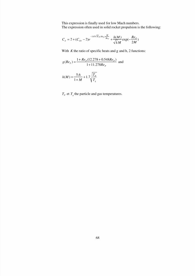
8/10/2019 Two phase flow in combustion system
http://slidepdf.com/reader/full/two-phase-flow-in-combustion-system 68/177
68
This expression is finally used for low Mach numbers.The expression often used in solid rocket propulsion is the following:
)2
exp()(
)2(2)(07.3
M
Re
M k
M heC C P Re
M RegK
dst d P
P
−+−+=−
With K the ratio of specific heats and g and h, 2 functions:
P
PP
P Re
Re Re Reg
278.111
)548.0278.12(1)(
+
++= and
g
P
T
T
M M h 7.1
1
6.5)( +
+=
PT et gT the particle and gas temperatures.
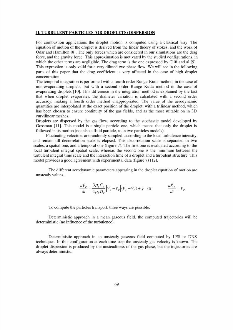
8/10/2019 Two phase flow in combustion system
http://slidepdf.com/reader/full/two-phase-flow-in-combustion-system 69/177
69
II. TURBULENT PARTICLES (OR DROPLETS) DISPERSION
For combustion applications the droplet motion is computed using a classical way. Theequation of motion of the droplet is derived from the linear theory of stokes, and the work ofOdar and Hamilton [8]. The only forces which are considered in our simulations are the drag
force, and the gravity force. This approximation is motivated by the studied configurations, inwhich the other terms are negligible. The drag term is the one expressed by Clift and al [9].This expression is only valid for a very diluted two phase flow. We will see in the followingparts of this paper that the drag coefficient is very affected in the case of high dropletconcentration.The temporal integration is performed with a fourth order Runge-Kutta method, in the case ofnon-evaporating droplets, but with a second order Runge Kutta method in the case ofevaporating droplets [10]. This difference in the integration method is explained by the factthat when droplet evaporates, the diameter variation is calculated with a second orderaccuracy, making a fourth order method unappropriated. The value of the aerodynamicquantities are interpolated at the exact position of the droplet, with a trilinear method, whichhas been chosen to ensure continuity of the gas fields, and as the most suitable on in 3D
curvilinear meshes. Droplets are dispersed by the gas flow, according to the stochastic model developed byGossman [11]. This model is a single particle one, which means that only the droplet isfollowed in its motion (not also a fluid particle, as in two particles models).
Fluctuating velocities are randomly sampled, according to the local turbulence intensity,and remain till decorrelation scale is elapsed. This decorrelation scale is separated in twoscales, a spatial one, and a temporal one (figure 7). The first one is evaluated according to thelocal turbulent integral spatial scale, whereas the second one is the minimum between theturbulent integral time scale and the interaction time of a droplet and a turbulent structure. Thismodel provides a good agreement with experimental data (figure 7) [12].
The different aerodynamic parameters appearing in the droplet equation of motion areunsteady values.
To compute the particles transport, three ways are possible:
Deterministic approach in a mean gaseous field, the computed trajectories will bedeterministic (no influence of the turbulence).
Deterministic approach in an unsteady gaseous field computed by LES or DNStechniques. In this configuration at each time step the unsteady gas velocity is known. Thedroplet dispersion is produced by the unsteadiness of the gas phase, but the trajectories arealways deterministic.
gV V V V D
C
dt
V d PgPg
PP
d gP rrrrrr
+−−= )(4
3
ρ
ρ (I) P
P V dt
X d rr
=

8/10/2019 Two phase flow in combustion system
http://slidepdf.com/reader/full/two-phase-flow-in-combustion-system 70/177
70
Stochastic or steady:
Numerical simulation of the gaseous fiels by RANS approach and a turbulencemodel using two equations: K et ε for example. This kind of computationgives for any mesh the mean flow field and the mean velocity fluctuationsthanks to the knowledge of the turbulent kinetic energy K and the dissipative
rate et la dissipation turbulente ε .
)wvu(2
1K
2'22' +′+=
x
u2K
3
2u t2
∂
∂
ρ
µ−=′
x
v2K
3
2v t2
∂
∂
ρ
µ−=′
x
w2K3
2w
t2
∂
∂
ρ
µ−=′
)x
v
y
u(vu t
∂
∂+
∂
∂
ρ
µ−=′′
The fluctuating velocities wvu ′′′ ,, must be modeled.An unsteady turbulent gaseous flow must be simulate from a stochastic model.The fluctuating velocity '
u will be randomly sampled such as:ut z y xU t z y xu ′+= ),,(),,( 0,000,00
idem for v and wThen the new position of the particle corresponding to the time 1t is computed
with the droplet equation of motion (I) using the previous equation. Thecomputation continue up to 0t t
i − < τ (interaction time), the new positions of
the particle ( iii z y x ,, ) are computed with the same fluctuating gaseous
velocity. Then a new fluctuating gaseous velocity is randomly sampledknowing the mean fluctuating velocities (Reynolds tensor) at the last positionof the particle.
Droplet dispersion model
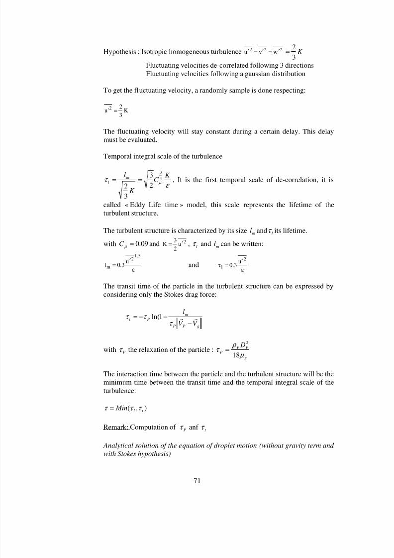
8/10/2019 Two phase flow in combustion system
http://slidepdf.com/reader/full/two-phase-flow-in-combustion-system 71/177
71
Hypothesis : Isotropic homogeneous turbulence 222 wvu ′=′=′ K 3
2=
Fluctuating velocities de-correlated following 3 directionsFluctuating velocities following a gaussian distribution
To get the fluctuating velocity, a randomly sample is done respecting:
K3
2'u 2 =
The fluctuating velocity will stay constant during a certain delay. This delaymust be evaluated.
Temporal integral scale of the turbulence
ε τ µ
K C
K
lm
l4
3
2
3
3
2 == , It is the first temporal scale of de-correlation, it is
called « Eddy Life time » model, this scale represents the lifetime of theturbulent structure.
The turbulent structure is characterized by its size ml and l
τ its lifetime.
with 09.0= µ C and 2u2
3K ′= , l
τ and ml can be written:
ε
′=
5.12
mu
3.0l andε
′=τ
2
lu
3.0
The transit time of the particle in the turbulent structure can be expressed by
considering only the Stokes drag force:
gPP
m
Pt
V V
lrr
−−−=τ
τ τ 1ln(
with Pτ the relaxation of the particle :g
PPP
D
µ
ρ τ
18
2
=
The interaction time between the particle and the turbulent structure will be theminimum time between the transit time and the temporal integral scale of the
turbulence:
),( t l Min τ τ τ =
Remark: Computation of Pτ anf
t τ
Analytical solution of the equation of droplet motion (without gravity term and
with Stokes hypothesis)
8/10/2019 Two phase flow in combustion system
http://slidepdf.com/reader/full/two-phase-flow-in-combustion-system 72/177
72
).......(36
3
PgPg
PP
P V V D
dt
V d D rrr
−= πµ π
ρ (I)
Hyp : we suppose CteV g =
r
New variable: PP V V V rrr
−=∆
)18
()0()(2PP
g
D
t EXPV t V
ρ
µ −∆=∆
rrsolution of (I)
Let: µ
ρ τ
18
2PP
P
D=
P
t
gPgP eV V V t V τ
−
−+= ).)0(()(
rrrr
Droplet transit time to cross the spatial integral scale of the turbulence: m L :
)1()0()(0
−∆−=∆=−
∫ P
t
t
eV dt t V LPPm
τ
τ τ
τ
))0(
1ln(V
L
P
m
Pt ∆
−−=τ
τ τ
References:
[8] ODAR, F, and HAMILTON, N , S, Forces on a sphere acceleration in a viscous fluidJ; Fluid Mech, vol 18, pp302-314, 1964
[9] CLIFT, R, GRACE, J, R, and WEBER, M, E, Bubbles, Drops and ParticlesAcademic Press, New York, 1978
[10] BEARD, P, BISCOS, Y, BISSIERES, D, LAVERGNE GExperimental and numerical studies of droplet dispersion in basic configurations of two phaseflows.
7
th
Workshop on two phase flow prediction - Erlangen 1994[11] GOSMAN, A, D, IOANNIDES, E Aspects of computer simulation of liquid fuelledcombustorsAIAA 81-0323, 19th Aerospace Sciences Meeting, Saint Louis, 1981.
[12] BEARD, P, BISSIERES, D, LAVERGNE, G, ROMPTEAUX, A, Experimental andnumerical studies of droplet turbulent dispersion in two phase flows.
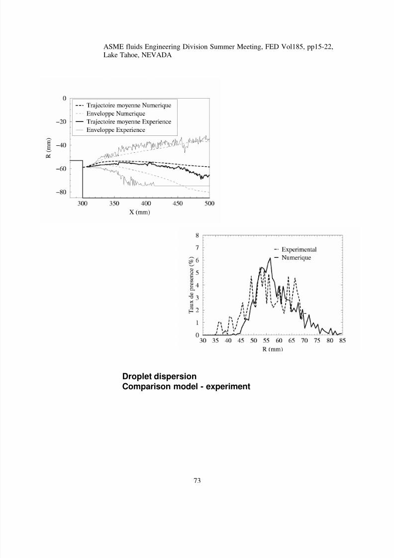
8/10/2019 Two phase flow in combustion system
http://slidepdf.com/reader/full/two-phase-flow-in-combustion-system 73/177
8/10/2019 Two phase flow in combustion system
http://slidepdf.com/reader/full/two-phase-flow-in-combustion-system 74/177
74
Chapter VII: Droplet evaporation andcombustion
8/10/2019 Two phase flow in combustion system
http://slidepdf.com/reader/full/two-phase-flow-in-combustion-system 75/177
75
EVAPORATION MODEL FOR AN ISOLATED DROPLET
We first consider the vaporisation of a motionless, cold, droplet after it is placed in a hot,stagnant, gravity-free environment of infinite extent. Assuming the system pressure is muchless than the critical pressure of the liquid, critical phenomena are not important. The lack of
forced or natural convection then implies the vaporisation of a spherical droplet as illustratedin figure 8 . Since the droplet temperature, in particular its surface value, is lower than that ofthe ambience, heat is transferred towards the droplet through conduction. At the surface, apart of this heat further transferred to the droplet interior causing the droplet to heat up. Therest is used to evaporate the liquid such that a high concentration of fuel vapour, generally atits saturation value, exists at the droplet surface.When the fuel vapour concentration in the environment is lower than that at the surface, aconcentration gradient exists through which the fuel vapour is transported outward. Thedepletion of the fuel vapour at the surface gives possible further evaporation. Thus, throughthe above mechanism, a liquid mass can be continuously converted to vapour and eventuallydispersed to the ambience i.e. droplet vaporisation is effected.The initial vaporisation rate is low because the droplet is cold. As the liquid temperature rises,
this rate will increase as a result of higher fuel vapour concentration at the droplet surface.This has two effects, an increasing portion of the energy reaching the droplet surface mustsupply the heat of vaporisation of the evaporating fuel, and the outward flow of fuel vapourreduces the rate of heat transfer to the droplet. This slows the rate of increase of the liquidsurface temperature and later in the process temperatures become more uniform in the liquidphase. For a pure liquid, droplet heating is mostly over in the early part of the droplet lifetimesuch that the subsequent rate of its surface area, or equivalently its diameter squared, remainsconstant with time, as predicted by the d2 law (see the following section). When a droplet issurrounded by a hot oxidising medium, it can ignite, giving rise to a reaction zone in itsimmediate vicinity. The resulting spherically- symmetric burning, shown in figure 8 , is of thediffusion flame type in which the outwardly-diffusing fuel vapour and the inwardly-diffusingoxidiser gas approach a reaction zone in approximately stochiometric proportion.The ensuing reaction is rapid and intense, implying the reaction zone is thin and very littlereactants can leak through the flame. The heat generated is transported both outward to theambience and inward for droplet heating and evaporation. Similar to the vaporisation case, fora pure fuel, much of the droplet heating is rapidly over and the droplet surface area thenregresses at a constant rate.In fact droplet burning bears many similarities with droplet vaporisation and apart from thegas-phase reactions, the detailed transport mechanisms within the droplet and the evaporationprocess at its surface are qualitatively the same in both cases. Thus during combustion, thedroplet simply perceives the flame as a hotter "ambience" located at a somewhat closerdistance. For the spherically-symmetric configurations shown in figure 8, only radial transportis possible. In the gas phase this transport consists of both diffusion and convection. In theliquid phase only diffusion exists. In the presence of either forced and/or natural convection, anon radial relative velocity exists between the droplet and the surrounding gas. The shearstress exerted by the gas flow on the surface induces recirculating motion within the droplet,leading to a pair of vortices as shown in figure. Beyond sufficiently strong blowing can leadto the extinction of the envelope diffusion flame or other effects occurring in multicomponentdroplet burning. Finally, if the flow Reynolds or Grashof number is large enough, separationoccurs close to the rear stagnation point such that wake regions are created as shown in figure8.
8/10/2019 Two phase flow in combustion system
http://slidepdf.com/reader/full/two-phase-flow-in-combustion-system 76/177
76
The above discussions show that droplet combustion primarily involves the heat, mass, andmomentum transfer processes in gas and liquid phases and their coupling at the interface. Ithad also to be recognised that the importance of kinetic effects in droplet burning is restrictedto critical phenomena as ignition and extinction.
Different configurations of burning droplets are shown on the figure 9.
Liquid phase calculation/Droplet heatingThe figure 10 illustrates the temperature profiles within a droplet for the three employeddroplet models and at three different time steps.
D2 law Model :
The d2 law model is the simplest possible model describing droplet vaporization andcombustion. It embodies much of the essential physics and yields crude estimates on thedroplet evaporation rate. The model deals with spherical symmetry for both liquid and gasphases. The droplet temperature is assumed to be uniform and remains constant at its wet-bulbvalue. The original model proposed by Godsave [13] also assumed constant properties in both
the gas and liquid phases, together with Lewis-number equal to unity. At the gas-liquidinterface, it is assumed that the fuel vapour mass fraction is a function of the surfacetemperature given by some equilibrium vapour pressure equation such as the Clausius-Clapeyron relation. It should be noted, that the D2-law Model neglects the liquid phase heatand mass transfer and is basically a gas-phase model.
Following, we recall the major assumptions applied in this case.
1. Spherical symmetry : forced and natural convection are neglected, whichreduces the analysis to one dimension.
2. No spray effects : the droplet is an isolated one immersed in an infiniteoxidising environment.
3. Diffusion being rate controlling4. Isobaric process5. Flame sheet combustion : chemical reaction rates are much faster than gas
phase diffusion rates that the flame is of infinitesimal thickness and can beand products.
6. Constant gas phase transport properties : the specific heats and thermalconductivity are constants and the Lewis is unity throughout. Theseassumptions cause considerable uncertainty in estimating the evaporationrate, wherefore more recent modelling allow for the effects of variablephysical properties.
7. Gas phase quasi-steadiness : because of the significant density disparitybetween liquid and gas, the liquid possesses great inertia such that itsproperties at the droplet surface, for example the regression rate, speciesconcentrations, and temperature, change at rates much slower than those ofthe gas phase transport processes.
8. Simultaneous fuel evaporation and consumption : this assumes that theamount of fuel evaporated at the surface is instantaneous consumed at theflame, or the instantaneous evaporation rate is equal to that of consumption.This neglects the change of the amount of fuel vapour present between thedroplet and flame as a result of the continuous variation of their physical
8/10/2019 Two phase flow in combustion system
http://slidepdf.com/reader/full/two-phase-flow-in-combustion-system 77/177
77
sizes as burning progresses. In order words, the effect of fuel vapouraccumulation is neglected.
9. Single fuel species : thus it is not necessary to analyse liquid phase masstransport.
10. Saturation vapour pressure at droplet surface : this is based on theassumption that the phase change process between liquid and vapour occurs
at a rate much faster than those for gas phase transport. Thereforeevaporation at the surface is at equilibrium, producing fuel vapour which isat its saturation vapour pressure corresponding to the droplet surfacetemperature.
11. No Soret, Dufour and radiation effects
I.1 Isolated droplet evaporation without convection
Continuity equation for species in spherical coordinates
wr dr
dY Dr
dr
d
r
Y vr F F 222 )( +=
∂
∂ ρ ρ (I)
Energy equation in spherical coordinates
qr dr
T dC r
C dr
d
dr
T dC vr P
P
P 222 )( += λ
ρ (II)
w et q are respectively the reaction rate and the heat of reaction
Balance continuity equation for the vapor phase at the droplet surface
−+= s
F
ssssF sss
dr
dY DvY v )()( ρ ρ ρ (III)
Total gas mass flux fuel mass flux fuel mass flux byLeaving the by convection diffusion at the droplet surfacesurface at the droplet
surface
We can deduce:1)(
)(
−=
sF
F
sY
dr
dY D
v (IV)
Spalding parameter:
S Fs
F
r r surfacetheat speciesothers for fraction Massr radiustheat fractionmassFuel
Y Y b
==
−=
........ ......1 (V)
Then ssdr
db Dv )(= (VI)
For evaporation alone : w=0
8/10/2019 Two phase flow in combustion system
http://slidepdf.com/reader/full/two-phase-flow-in-combustion-system 78/177
78
(I) become: )( 22
dr
db Dr
dr
d
dr
dbvr ρ ρ = (VII)
∞=r
1−
==
=
∞∞
∞
Fs
F
F F
Y
Y bb
Y Y
(VIII)
Then with continuity equation
sss vr Ctevr ρ ρ 22 == (IX)
After integration of equation VII:
[ ]1)(ln +−= ∞ s
s
ss bb D
vr (X)
The difference sbb −∞ is called Spalding transfer number
FS
F Fs
sY
Y Y bb B
−
−=−= ∞
∞ 1 (XI)
(X) gives : )1ln( B Dvr sss
+= (XII)
The mass flow rate/unit of area is designed by F G
ss
s
F
F vr
mG ρ
π ==
24
& (XIII)
The evaporation rate can be expressed by:
s
ss
s
F
F r
B D
r
mG
)1ln(
4 2
+== ρ
π
& (XIV)
Then we must compute FsY :
Hypothesis: The gas at the droplet surface is saturated by the vapor coming from thedroplet evaporationWe must determine the droplet temperature surface
sT
We consider the energy equation (II) with Q=0.
)( 22
dr
dT r
dr
d
dr
dT C vr
Psss λ ρ = (XV)
Limit conditions at the droplet surface :
8/10/2019 Two phase flow in combustion system
http://slidepdf.com/reader/full/two-phase-flow-in-combustion-system 79/177
79
vsss hv
dr
dT ∆= ρ λ )( ss
T r r T == )( (XVI)
By neglecting the conduction inside the droplet the integration of (XV) gives :
dr
dT r
C
hT T C vr
P
v
sPsss λ ρ 22 )( =∆
+− (XVII)
After variables separation method and by considering ∞= T T for ∞= r r and sr r = for
the surface, andPC
a ρ
λ α ==
)1ln()(
1ln T s
v
sP
sss Bh
T T C vr +=
∆
−+= ∞ α α (XVIII)
After comparison (XVIII) and (XII) :
−
−+=
∆
−+= ∞∞
11ln
)(1ln
Fs
FsF
s
v
sP
sssY
Y Y D
h
T T C vr α (XIX)
[ ] [ ] M sT sss
B D Bvr +=+= 1ln1lnα (XX)
if )1( == Le Dssα M T B B =
1_)_(−
=∆
∞∞
Fs
FsF
v
sP
Y
Y Y
h
T T C (XXI)
This equation linked the two unknowns sT et Fs
Y , another equation is needed
W
W
P
P
nW
W nY F F F F F
F === ρ
ρ (XXII)
Clapeyron equation:
2lns
vF
RT h
dT Pd ∆= (XXIII)
)11
(lnsref
v
Fref
F
T T R
h
P
P−
∆= (XXIV)
Equations XXI, XXII, XXIV give the following parameters: F sFs PT Y ,,
8/10/2019 Two phase flow in combustion system
http://slidepdf.com/reader/full/two-phase-flow-in-combustion-system 80/177
80
The number B and the vapor mass can be calculated from equations XI and XIV.
Droplet evaporation time vτ :
- Droplet continuity equation :
ss
s
l vdt
dr
ρ ρ =− (XXV)
From equation XIV
)1ln( Br
D
dt
dr
sl
sss +−= ρ
ρ (XXVI)
After integration :
t B
d d
l
ss
ρ
α ρ )1ln(820
2 +−= (XXVII)
By comparing (XXVII) with t d d v β −= 2
02
)1ln(8
Bl
ss
v +=
ρ
α ρ β (XXVIII)
v
vv
d t
β τ
20==
The evaporation rate is expressed by the liquid mass variation with time.
)1
1ln(2
s
gY
Y D Dp
dt
dmp
−
∞−−= ρ π
With ∞Y the vapour mass fraction at the infinite, Ys the vapour mass fraction at the dropletsurface, D the diffusivity coefficient, Dp the droplet diameter and rg the gas density
Then we can write :
)1
1ln(2
22
s
g pPY
Y D Dp
dt
dDp D
−
∞−−= ρ π
π ρ
Then : )1
1ln(
82
sP
gP
Y
Y D
dt
dD
−
∞−−=
ρ
ρ
t C D DePP −= 2
02 with )
1
1(
8
S P
g
eY
Y Ln
DC
−
∞−=
ρ
ρ

8/10/2019 Two phase flow in combustion system
http://slidepdf.com/reader/full/two-phase-flow-in-combustion-system 81/177
81
It is very simple to use this expression to get the evaporation rate, the vapour mass fraction atthe droplet surface is obtained from the vapour pressure at the droplet surface Psat (Tp) withthe following relation :
P
T P X Psat
fs
)(=
g fs f fs
f fs
fs M X M X
M X Y
)1( −+=
The Spalding mass transfer number BM and thermal transfer number BT are introduced tocharacterize mass and thermal transfer at the droplet surface.
s
s M
Y
Y Y B
−
∞−=
1
V
PG
T L
TsT C B
)( −∞=
With Lv is the latent vaporisation of the liquid
The evaporation rate can be expressed by :)1ln(2
M gP B D D
dt
dmp+−= ρ π
)1ln(2 T
Pg
g
P BC
Ddt
dmp+−=
λ π
Then :
Le
T M B B )1()1( +=+
Le is the Lewis number and equal to 1, then we find T M B B =
In the application, the values of these two parameters can be slightly different, in this caseif M r B B > , this mean that the thermal exchange is higher than the mass exchange, the droplettemperature should be increase. If M r B B < , it should be decreases. We have to determine the
droplet temperature to get T M B B = and then to have Lewis number equal to 1 (to verify thehypothesis).
I.2 Variable physical properties
Hypothesis number 6 assumes constant gas physical properties and Le = 1. To improve thecomputation of heat and mass exchanges, a vapour film at the droplet surface is considered.Exchanges are computes in considering reference parameters for the gas phase.Hubbard [16] uses the 1/3 rule to determine the vapour temperature and vapour mass fraction:
3
2)(
3
1 ∞+=−∞+=
T T T T T T P
PPref
8/10/2019 Two phase flow in combustion system
http://slidepdf.com/reader/full/two-phase-flow-in-combustion-system 82/177
82
3
2)(
3
1 ∞+=−∞+=
Y Y Y Y Y Y s
ssef
All the physical properties are determined by using these two reference parameters ref T and
ref Y .
For example the Lewis number will expressed by :ref pref ref
ref ref
DC Le
ρ
λ =
And then :
)1(2 M ref ref P B Ln D Ddt
dmp+−= ρ π
)1()(
2 T
ref PV
ref
P B LnT C
Ddt
dmp+−=
λ π
BM and BT are related by :
)()1()1( ref
ref T Cpv
Cpref Le
T M B B +=+
The exponent of the last expression should be equal to 1 to have T M B B =
I.3 Convection correctionForced convection, resulting from a slip velocity between the droplet and the surrounding gas,increases the heat and mass transfer at the droplet [17,18]. This phenomenon is treated byintroducing corrected values for the Nusselt and Sherwood number :
ss
r
r T T
r
t
Nus
2 / )(
)(
∞−∂
∂−
= andsF Fs
r F
r Y Y
r
Y
Shs
2 / )(
)(
∞−∂
∂−
=
Which describe the non dimensional temperature and concentration gradients at the dropletsurface.First Ranz Marchall approach :
t K d d o
'22 −= with )Pr3.01( 3
1'
eP RK K += and v
K β =
g
Pgg
eP
d uu R
µ
ρ −= particular Reynolds number
8/10/2019 Two phase flow in combustion system
http://slidepdf.com/reader/full/two-phase-flow-in-combustion-system 83/177
83
g
g
r a
Pυ
= Prandtl number with gυ : cinematic viscosity of gas and ga : thermal
diffusivity of gas
Pgg
g
gC
a ρ
λ =
This proceeding and the associated empirical correlation used for convection correction aredescribed in the following :
The convection correction applied to this work refers to the approach of Abramzon andSirignano where the actual Nusselt and Sherwood numbers are given by :
T
T
B
B Ln Nu Nu
)1(* += and
M
M
B
B LnShSh
)1(* +=
Nu* and Sh* denote modified convection corrected values of the transfer coefficients, whichinclude the effect of droplet vaporisation.
They are expressed as :
)(
22 0*
T BF
Nu Nu
−+= and
)(
22 0*
M BF
ShSh
−+=
Where 0 Nu and 0Sh describe the heat and mass transfer coefficients for a solid non vaporisingspherical particle in a flowing fluid :
)(Pr)1(1 3
1
0 Re f Re Nu ++= and )()1(1 3
1
0 Re f ReScSh ++=
1)( = Re f for Re 1≤ and 077.0)( Re Re f = for 1 400≤≤ Re
The function F represents the correction due to droplet vaporisation and was analyticallyobtained by using the boundary layer theory under consideration of vaporisation phenomena :
B
B Ln B BF
)1()1()( 7.0 +
+=
0 / )(
T T T BF δ δ =
0 / )(
M M M BF δ δ =
Where δT, δM are respectively the thermal and mass film thickness which pilot the exchangesduring the evaporation.
These parameters can also be written : 20 −=
Nu DP
T δ
20 −=
Sh
DP
M δ
Or,T
P D Nu
δ += 20 and
M
P DSh
δ += 20

8/10/2019 Two phase flow in combustion system
http://slidepdf.com/reader/full/two-phase-flow-in-combustion-system 84/177
84
Now the evaporation rate can be written :
)1(* M ref ref P
P B LnSh D Ddt
dm+−= ρ π
)1()(*
T
ref pv
ref P B Ln Nu
T C D +− λ π
We recall that Pr and Sc are the Prandtl and Schmidt numbers λ µ / Pr pC =
Sc = D ρ
µ and Re the Reynolds number : Re =
µ
ρ PVD∆
I.4 LIQUID PHASE MODEL
• D2 model :This model assumes a constant temperature over the whole droplet diameter, there is no heat
flux into the droplet. Consequently the total energy flux H from the gas phase to the dropletsurface is used for droplet vaporisation, so :
H = Lv where Lv is the specific latent heat of vaporisation and H represents the heat flux permass of evaporated fuel.
• Infinite ConductivityIn this case the heat conduction is considered extremely rapid in comparison with thermal andmass exchanges around the droplet. The droplet temperature is uniform Tp = T l but will betime dependant Tl (t).The enthalpy balance gives :
V P
gl Ldt
dmQQ +=
gQ is the heat flux coming from the gas phase, l
Q is heat flux for droplet heating and
V P L
dt
dmthe heat flux for droplet evaporation.
)(2PPg
T T h DQ −= ∞π
)( Pref Pg T T Nu DQ −= ∞λ π
T
T
Pref Pg B
B Ln
T T Nu DQ
)1(
)(* +
−= ∞λ π
T
Pref Pg
B
T T T Cpv
dt
dmQ
))(( −−=
∞
])((
[ V
T
Pref pvP
l L B
T T T C
dt
dmQ −
−−=
∞
8/10/2019 Two phase flow in combustion system
http://slidepdf.com/reader/full/two-phase-flow-in-combustion-system 85/177
85
and
dt
dm
Q L
T T T C B
P
l
V
Pref pv
T
−
−=
∞ ))((
In this case :
dt
dT C
DQ l
PllP
l ρ π 6
3
=
and :
PllP
ll
C D
Q
dt
dT
ρ π 3
6=
• Limited conductionThe conduction Limit Model modifies the infinite conductivity model by assuming a finitethermal conductivity, leading to a non uniform temperature distribution T(r,t) within thedroplet. In this model, the temperature at the droplet surface Ts is influenced by the heat fluxfrom the flame front to the droplet surface[19].The energy conservation equation gives :
)(1 2
2 r
T r
r r t
T l
l
l
∂
∂
∂
∂=
∂
∂α
and the boundary conditions : r = 0 : 0=∂
∂
r
T l and 0)0,( ll T t r T ==
r = rs : sl T T = and for symetry reason :
r
T r Q l
lPl∂
∂= λ π 24
Thus the gas phase coupling is provided by the droplet surface temperature Ts
• Effective conductionThe gas phase convection around the droplet induces recirculating zones inside the liquid,called Hill vortex [18,20].To take into account this effect a corrective factor χis used for the heat conduction coefficient.
χ λ λ lref =
with ]30
log245.2tanh[86.086.1 elP+= χ and lPsPllel
DU C P λ ρ / =
and F
PP
l
ms C
ReV V
U 32
rr−
= µ
µ
8/10/2019 Two phase flow in combustion system
http://slidepdf.com/reader/full/two-phase-flow-in-combustion-system 86/177
86
3
2
69.12 −
= PF ReC for 10 100≤≤ P Re
ValidationIn order to check the validity of these droplet evaporation models, computed results
have been compared with those of other authors [21]. Examples of results are shown on the
figure 11. The chosen configuration is the one used by Abramson and Sirignano [18].The numerical simulation is very easy for the infinite conductivity model :
dT/dt = (T(t + δt) – T(t))/ δt
For the others models, Crank Nicholson scheme is used (order 2).Evaporation and combustion of an isolated droplet
Continuity equation for species in spherical coordinates
• For the Fuel
F F
F F wr
dr dY Dr
dr d
r Y vr 222 )( +=∂
∂ ρ ρ (I)
(I)• For Oxygen
O
O
O
O wr dr
dY Dr
dr
d
r
Y vr 222 )( +=
∂
∂ ρ ρ (II)
• For the products
P
P
P
P wr dr
dY Dr
dr
d
r
Y vr 222 )( +=
∂
∂ ρ ρ (III)
• Energy equation in spherical coordinates
qr dr
T dC r
C dr
d
dr
T dC vr P
P
P 222 )( += λ
ρ (IV)
w et q are respectively the reaction rate and the heat of reaction
Continuity equation Ctevr = ρ 2 (V)
The solution of this problem induces the determination of the evaporation rate, the flameposition, concentration and temperature profiles.
Considering a global scheme for the chemical kinetics : very fast combustion
The stoechiometric equation is written by:
8/10/2019 Two phase flow in combustion system
http://slidepdf.com/reader/full/two-phase-flow-in-combustion-system 87/177
87
f gms of Fuel, F + 1 gm d’Oxygen, O → (1+f) gms of products, P + f ∆H cals of heat (VI)
f is the stoechiometric coefficient (grams of Fuel per gram of Oxygen), ∆H is the heat ofreaction (calories par gram de Fuel). This stoechiometric reaction linked source terms by thefollowing equations:
H f
q
f
w
w f
w P
O
F
∆+=+=−=− 1 (VII)
Recall : the consumption of reactants and the production of the products are linked by:
AA + bB + ….⇒mM + nN + …
with : =−=−==−=−dt
dC
ndt
dC
mdt
dC
bdt
dC
a
N M B A 11........
11
And iC the concentration of specie i.
(VII) shows that : 0=∆+ F Hwq
(VIII)
By multiplying (I) by ∆H and adding it to (IV), we obtain:
[ ] 0)()( 22 =
∆+−
∆+
dr
HY T C d r v
dr
HY T C d r
dr
d F P
sss
F P ρ ρ α with F D=α
By dividing this last equation by the constant: )( FlFs Y Y H Q −∆+ , we find again an equation
identical to VII obtained for the case of droplet evaporation alone:
[ ] 022 =−dr
dbr v
dr
dbr
dr
d FT
sss
FT ρ ρα (IX) with)(
)()(
FlFs
F F P
FT Y Y H Q
Y Y H T T C b
−∆+
−∆+−= ∞∞
0=∞F Y for a diffusion flame
Limit conditions for equation IX :
s
P
ssQ
T T C
dr
d v )
((
∞−= ρα ρ
s
FlFs
F F
F ssY Y
Y Y
dr
d Dv )(
−
−= ∞ ρ ρ
By multiplying this last expression by H ∆ :
s
Pg
ssdr
T dC Qv )( ρα ρ =
By adding these two equations and knowing that F D=α , we obtain the following limitcondition:
sF
F FlFsssdr
HY d DY Y H v )()(
∆=−∆ ρ ρ
8/10/2019 Two phase flow in combustion system
http://slidepdf.com/reader/full/two-phase-flow-in-combustion-system 88/177
88
s
FT
ssdr
dbv )( ρα ρ = (X)
FT b is the conservative variable for this problem of combustion
When O D=α , we can verify that the conservative equations of energy and oxygen can be
reduced to an equation identical to IX if the limit condition is of X type and if theconservative variable OT
b is defined by:
Q
Y Y Hf T T C b
OOPg
OT
)()( ∞∞ −∆+−=
If OF D D = , the equations of oxygen and fuel are combined to a third equation defines by:
FlFs
OOF F
FO Y Y
Y Y f Y Y
b −
−−−
= ∞∞ )()(
(XI)
Then FOOT FT bbb ,, satisfy the following equations:
[ ] 022 =−dr
dbr v
dr
dbr
dr
d sss
ρ ρα
sssdr
dbv )( ρα ρ =
The solution of this equation is determined of the same manner than for droplet evaporationalone.
The b profile is given by:
r
r v
bb
B sss
s
1)
1
1ln(
2
ρα
ρ =
+−
+ (XII) by eliminating ρα ρ / sss
r v ,
)1()1()1( r
r
s
s
Bbb−
+=+− (XIII)
The mass transfer rate is given by equaling sr r = and sbb = in the equation XII.
)1ln( Br
vs
ss += ρα
ρ (XIV)
The mass transfer B is defined by the three equivalent following expressions:
FT FOOT B B B B === then OF
D D ==α

8/10/2019 Two phase flow in combustion system
http://slidepdf.com/reader/full/two-phase-flow-in-combustion-system 89/177
89
)(
)(
lsPlv
sPgO
OTsOT OT T T C h
T T C HfY bb B
−+∆
−+∆=−=
∞∞
∞ (XV)
FsFl
FsO
FOsFOFO
Y Y
Y fY bb B
−
+=−= ∞
∞ (XVI)
)()(
)(
FlFslsPlv
sPgFs
FTsFT FT Y Y H T T C h
T T C HY bb B
−∆+−+∆
−+∆−=−=
∞
∞ (XVII)
The suppression of the non linear sources terms in the conservative equations simplify theproblem of the diffusion flame. This technique is well known in the literature by the Schab-
Zeldovic transformation.The previous equations will be applied to find the mass transfer rate, the flame position andthe species and temperature profiles.
Combustion rate computation
If B is known, the burning rate can be computed from equation XIV. The Bcomputation requires the knowledge either s
T or FsY . By equaling FO
B and OT B ,
)(
)(
lsPlv
sPgO
FsFl
FsO
T T C h
T T C HfY
Y Y
Y fY
−+∆
−+∆=
−
+ ∞∞∞ (XVIII)
This last equation associated to the equation of the fuel saturated vapor (Clapeyron relation)determine s
T et B.
It is common to consider that Bs T T = (Boiling temperature) and to calculate OT
B for B :
)(
)(
l BPlv
BPgO
T T C h
T T C HfY B
−+∆
−+∆≈
∞∞ (XIX)
IF )( l BPl T T C − and )( BPg T T C −∞ are neglected, the B simplified expression is written:
v
O
h
HfY B
∆
∆≈ ∞
This approximation can induce a maximum error around 20% on the burning ratecomputation.
These equations (from XIV) show that the burning rate increases when the droplet size is
reduced and for an increasingPg
g
C
λ and B. The burning rate is high if the environment is hot
and enriched with oxygen and if the fuel is preheated. A fuel with high values of the reactionheat and the latent heat of evaporation will induce an efficient combustion.
8/10/2019 Two phase flow in combustion system
http://slidepdf.com/reader/full/two-phase-flow-in-combustion-system 90/177
90
Flame positionIn the flame the fuel and oxydiser concentrations are in the stoechiometric proportions andthe reaction is fastBy designing the flame position by the index c, OcFc
fY Y = By introducing this relation in XII and by simplifying with the help of equations XI andXVI, the flame radius is obtained and is written by:
) / 1ln(
12
FlO
sss
cY fY
r vr
∞+=
ρα
ρ , (XX)
ρα
ρ s
ss r v
=1, by using XIV :
)1ln(
)1ln(
+
+=
∞
Fl
Os
c
Y
fY
B
r
r (XXI)
This equation shows that for high burning rate, the flame will be far away the dropletsurface. If B is always greater than FlO
Y fY / ∞ , the diffusion flame will never reach the
droplet surface.
Example : for hydrocarbons, the ratio fuel/oxydizer f=0.32, if the liquid is pure ( 1=FlY )
and if it burns in standard air ( 232.0=∞OY ), equation XXI can be written :
)1ln(14 Br
r
s
c +≈
- Temperature profile
We suppose that between the droplet surface and the flame ( cs r r r << ), oxygen is
totally burnt and that outside the flame ( ∞<< r r c ), the fuel is also totally burnt. In thiscase )(r b
OT gives the temperature profile inside the flame and )(r bFT gives the profiletemperature outside the flame.
For cs r r r <<
With these hypothesis, the equations XII, XIV et XIX permit to get the temperatureprofile:
−+=−
−
1)1()()1(
r
r
sPg
s
BQT T C (XXII)
For ∞<< r r c , following the same previous procedure, we get:
Fl
O
FlOsPg
scPg
Y
fY
Y Q H fY T T C T T C
∞
∞∞
+
−∆+−=−
1
) / ()()( (XXIII)
This last expression can be applied with the respect of the following hypothesis:
8/10/2019 Two phase flow in combustion system
http://slidepdf.com/reader/full/two-phase-flow-in-combustion-system 91/177
91
- PgC in not dependent of the temperature and composition
- H ∆ is independent of the temperature- The Lewis number is equal to1 ( OF g
D D ==α )
The flame temperature is function of B, l BFlO T LT T f Y Y ,,,,,, ∞∞
- Fuel and oxygen mass fraction profile Profiles
The same procedure is followed to derive the equations of fuel and oxygen profiles.
For the Fuel:
∞∞ −−−+= OsssOFlF fY r r v fY Y r Y ρα ρ / )(exp1)()( 2 (XXIV)
For the Oxygen:
[ ] ∞∞ +−−
+= Osss
OFl
O Y r r v f
fY Y r Y 1 / )(exp
)()( 2 ρα ρ (XXV)
- Combustion time
The combustion time for one droplet is given from the decrease of the droplet diameter:
t d d b
λ −= 20
2 with the combustion rate bλ given by :
)1ln(8
Bl
b += ρ
ρα λ
Combustion time :b
b
d t
λ
20=
For hydrocarbons burning in air, the value of bλ is around scm / 10 22−
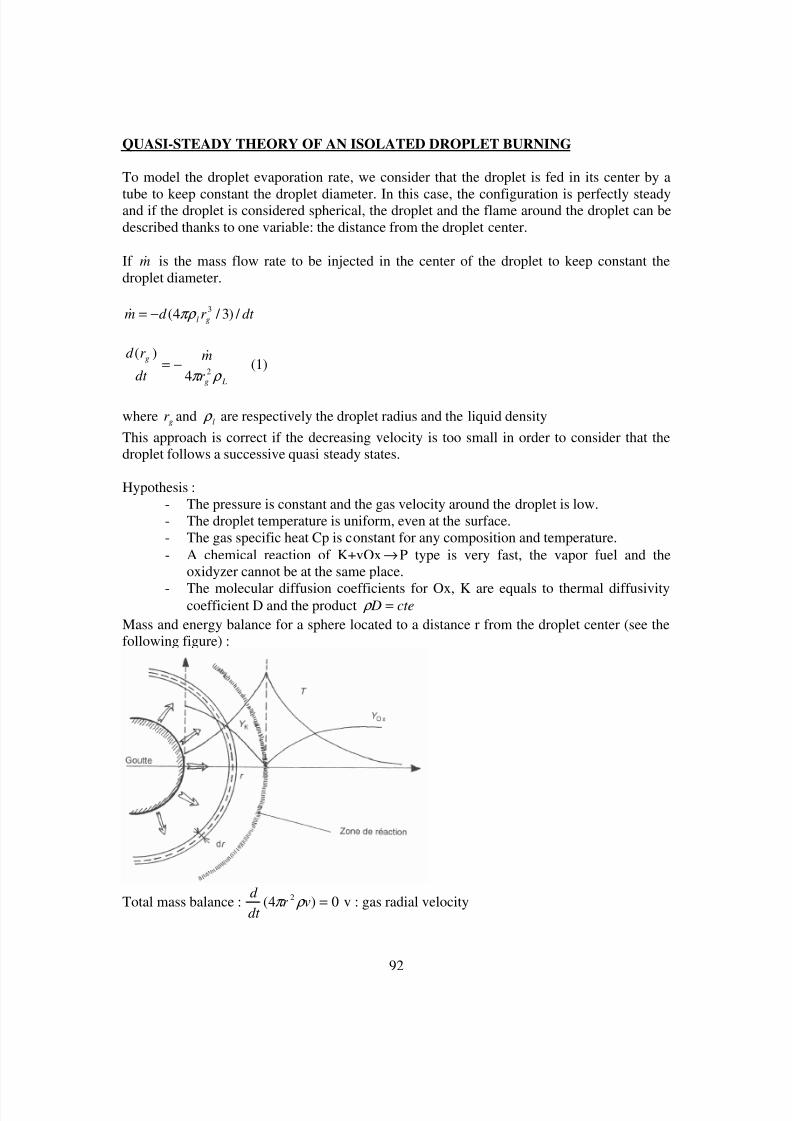
8/10/2019 Two phase flow in combustion system
http://slidepdf.com/reader/full/two-phase-flow-in-combustion-system 92/177
92
QUASI-STEADY THEORY OF AN ISOLATED DROPLET BURNING
To model the droplet evaporation rate, we consider that the droplet is fed in its center by a
tube to keep constant the droplet diameter. In this case, the configuration is perfectly steadyand if the droplet is considered spherical, the droplet and the flame around the droplet can bedescribed thanks to one variable: the distance from the droplet center.
If m& is the mass flow rate to be injected in the center of the droplet to keep constant thedroplet diameter.
dt r d mgl / )3 / 4( 3πρ −=&
Lg
g
r
m
dt
r d
ρ π 24
)( &−= (1)
where gr and l ρ are respectively the droplet radius and the liquid density
This approach is correct if the decreasing velocity is too small in order to consider that thedroplet follows a successive quasi steady states.
Hypothesis :- The pressure is constant and the gas velocity around the droplet is low.- The droplet temperature is uniform, even at the surface.- The gas specific heat Cp is constant for any composition and temperature.- A chemical reaction of K+vOx →P type is very fast, the vapor fuel and the
oxidyzer cannot be at the same place.
- The molecular diffusion coefficients for Ox, K are equals to thermal diffusivitycoefficient D and the product cte D = ρ Mass and energy balance for a sphere located to a distance r from the droplet center (see thefollowing figure) :
Total mass balance : 0)4( 2 =vr dt
d ρ π v : gas radial velocity
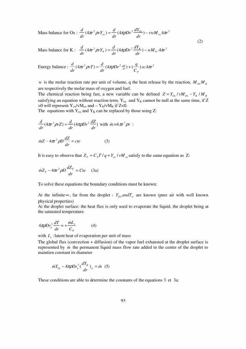
8/10/2019 Two phase flow in combustion system
http://slidepdf.com/reader/full/two-phase-flow-in-combustion-system 93/177

8/10/2019 Two phase flow in combustion system
http://slidepdf.com/reader/full/two-phase-flow-in-combustion-system 94/177
94
K M
m
dr
dZ Dr Z m
&& −=− ρ π 24 (6)
et
q
Lm
q
T C m
dr
dZ Dr Z m vgPT
T
&&& −−=− ρ π 24 (6a)
Z et ZT are obtained after integration of these two equations (function of r)
Using the boundary condition 0=∞K Y and thenOx
Ox
vM
Y Z
∞=∞
,)( , we get :
)4
exp()(
( ,)
Dr
m
q
L
vM
Y
q
T T C
q
L
q
T C Z v
Ox
OxgPvgP
T πρ
&−++
−+−=
∞∞ (7a)
)4
exp()1
(1 ,
Dr
m
M vM
Y
M Z
K Ox
Ox
K πρ
&−++−=
∞ (7)
These equations permit to determine the following profiles T Y Y K Ox ,, versus r around the
droplet depending of Tg (droplet temperature surface) and m& but these two last quantitiesmust be evaluated.The evaporation at the droplet surface induces a link between gK g
andY T , (gas mass fraction at
the droplet surface) and the pressure around the droplet: partial pressure of K which is equalto the pressure of the saturated vapor corresponding to the temperature T g. If gK
Y , is equal to
1, none product of the combustion can diffuse up to the droplet surface. This condition can bewritten )( pT T vapg = , the droplet evaporation temperature at the chosen. In real conditions,
gK Y , is slightly less than 1, and then g
T slightly less than )( pT vap .
Writing the relation for evaporation equilibrium:
P
gK
K
gK
K
gK
gs
M
Y
M
Y
M
Y
pT p)1(
)(,,
,
−+
= (8)
where the right term represents the molar fraction of the fuel vapor at the droplet surface , thelast equation is obtained giving Tg and gK Y , , the function Ps(T) is known.
m& can be now computed. The two equations 3 and 3a are associated to the three boundaryconditions: values of andZ Z T at the infinite, and the relation 8. The supplementary boundary
condition permits to compute m& . m& can be express either versus ,,gK Y either versus .gT
In the first case m& is computed from 7 expressed with r= gr , that gives:
K
gK
K
Ox
Ox
K
gg
M
Y
M
M
Y
M
r D
m
,
,
1
1
ln4
−
+
=
∞
ν
πρ
& (9)

8/10/2019 Two phase flow in combustion system
http://slidepdf.com/reader/full/two-phase-flow-in-combustion-system 95/177
95
In the second case, the relation the relation 7a is written for the droplet surface:
1
)(
ln4
,
+
+−
=
∞
∞
v
Ox
Ox
gP
gg L
M
qY T T C
r D
m ν
πρ
&
(9a)
In the both relations, gK getY T , can be computed independetly of m& and using 8 et the equality
9 and 9a .From the relations 7 et 7a, )()(),( r andT r Y r Y
K Ox can be plotted.
A new variable is defined z is defined such as )4 / exp( Dr m z πρ &−= which is equal to 1 for
r= ∞ , and at )4 / exp( gggg r Dm z πρ &−= for gr r = (where g D is the D value at the droplet
surface), the profiles of andT Y Y K Ox , are linear versus z.
The radius of the reaction surface F r is computed easily: 0==OxK
Y Y , and then Z=0.
lnF gg
K
K Ox
Ox
r D
m
M
M M
Y
πρ
ν
41
1,
&=
+∞
taking into account 9a ,g
F
r
r is obtained independently of m& :
)1ln(
)
)(
1ln(
,
,
Ox
K Ox
V
Ox
Ox
gP
g
F
M
M Y
L
M
qY T T C
r
r
ν
ν
∞
∞
∞
+
+−
+
= (10)

8/10/2019 Two phase flow in combustion system
http://slidepdf.com/reader/full/two-phase-flow-in-combustion-system 96/177
96
The maximum temperature F T , on the reaction surface can be deduced from 7a and 7 with
Z=0 and
: / qT C Z F PT =
Ox
K Ox
Ox
Ox
PP
v
g
Ox
K Ox
OxP
Ox
P
V
g
P
V
gF
M
M Y
M
Y
C
q
C
LT T
M
M Y
M C
qY
C
LT T
C
LT T
ν
ν
ν
ν
∞
∞
∞
∞
∞∞
+
+−+
=
+
++−
+−=,
,
,
,
1
)(
1
(11)
From equations 1 to 9 the decrease of the droplet diameter can be computed, consideringknown the droplet temperature g
T . This last value depends of the accuracy of the thermal
behavior of the droplet. Generally three main models are used: the 2 D law (the droplettemperature is considered constant at any point in the liquid and equal to the saturated
temperature, this simple model is often used but the heating phase of the droplet is notmodeled. Now in the new configurations of the burners the characteristic time of the heatingphase cannot be considered negligible. The second model is the infinite conduction model, inthis case a radial temperature gradient is considered and the third case corresponding to theeffective conduction model, the coefficient of conduction is modified by taking into accountvortices inside the droplets induced by the gas shear flow at the droplet surface.
References:
[13] GODSAVE, G, A, E, Studies of the combustion of drops in a fuel spray ; the burning ofsingle drops of fuelFourth Symposium (Int) on combustion (1953)
[14] LAW, C, K, Some recent advances in droplet combustionTechnical report, American Institute of Physics, 1989.
[15] SIRIGNANO, W, A, Fluid Dynamics of spraysJournal of fluid engineering 115: 345-378, 1993
[16] HUBBARD, B.,L, DENNY, V, E, and MILLS, M, F, Droplet evaporation ; effects oftransient and variable propertiesInt Journal Heat Mass Transfer 18, pp1003-1008, 1975
[17] ABRAMZON, B, and SIRIGNANO, W, A, Approximate theory of a single dropletvaporization in a convective field. Effects of variable properties, Stefan flow and transcientliquid heatingASME-JSME, Honolulu, 1987
[18] ABRAMZON, B, SIRIGNANO, W, A, Droplets vaporisation model for spraycombustion calculationsInt Journal Heat Mass Transfer 32 (9), pp1605-1618 (1981)

8/10/2019 Two phase flow in combustion system
http://slidepdf.com/reader/full/two-phase-flow-in-combustion-system 97/177
97
[19] AGGARWAL, S, K, TONG, A, Y, and SIRIGNANO, W, A,A comparison of vaporisation models in spray calculationsAIAA Journal, 22 (10) : pp 1448-1457, 1983.

8/10/2019 Two phase flow in combustion system
http://slidepdf.com/reader/full/two-phase-flow-in-combustion-system 98/177
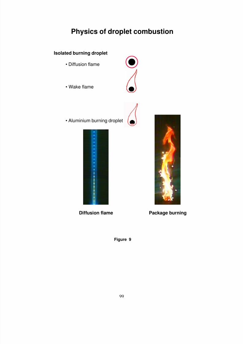
8/10/2019 Two phase flow in combustion system
http://slidepdf.com/reader/full/two-phase-flow-in-combustion-system 99/177
99
Figure 9
Physics of droplet combustion
Isolated burning droplet
• Diffusion flame
• Wake flame
• Aluminium burning droplet
Diffusion flame Package burning
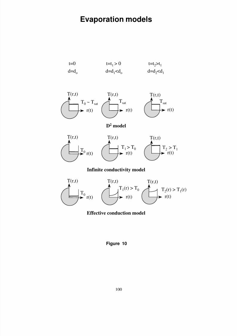
8/10/2019 Two phase flow in combustion system
http://slidepdf.com/reader/full/two-phase-flow-in-combustion-system 100/177
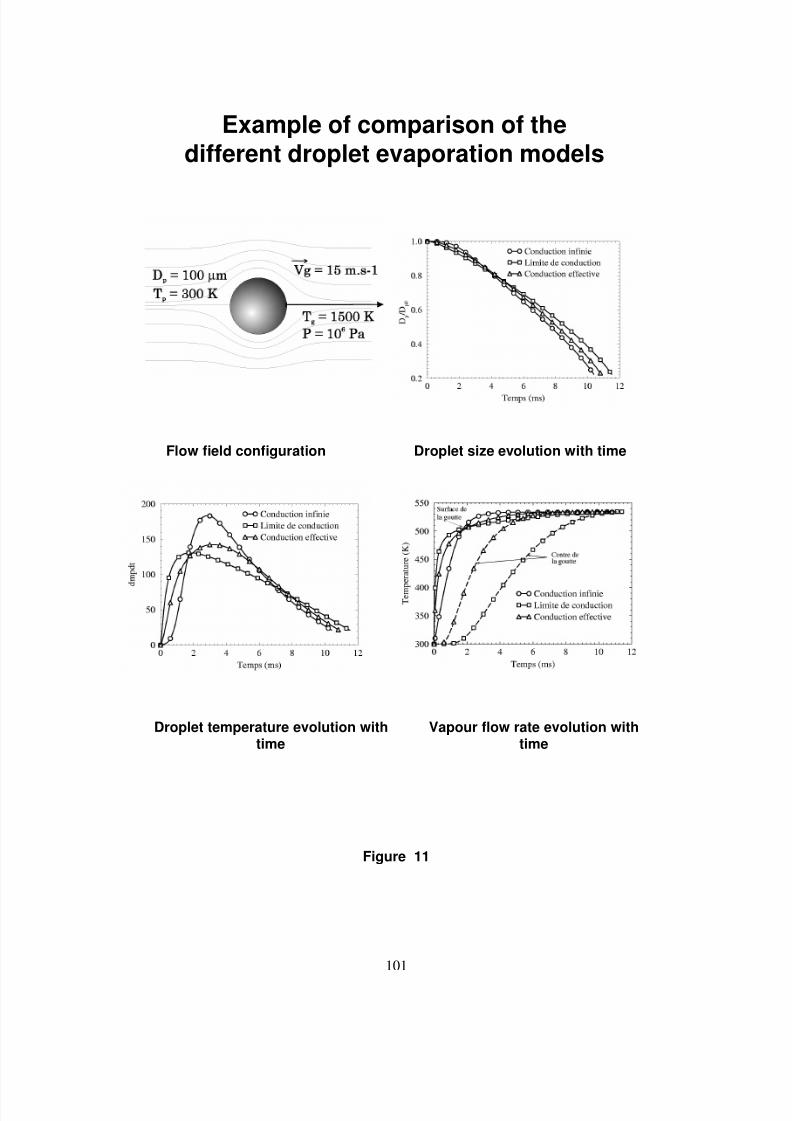
8/10/2019 Two phase flow in combustion system
http://slidepdf.com/reader/full/two-phase-flow-in-combustion-system 101/177
101
Figure 11
Example of comparison of thedifferent droplet evaporation models
Flow field configuration Droplet size evolution with time
Droplet temperature evolution withtime
Vapour flow rate evolution withtime

8/10/2019 Two phase flow in combustion system
http://slidepdf.com/reader/full/two-phase-flow-in-combustion-system 102/177
102
Chapter VIII Dense sprays

8/10/2019 Two phase flow in combustion system
http://slidepdf.com/reader/full/two-phase-flow-in-combustion-system 103/177
103
The previous theories are valid for isolated droplet but in the case of sprays in some regionsthe droplet concentration can be high and the evaporation rate or the burning rate mustcorrected. Different combustion regimes can be appeared in the spray depending on the localdroplet concentration (or depending of the droplets spacing parameter):
Isolated burning droplet
Droplets package burning (internal or external)Diffusion flame around the spray
In this chapter, two classification regimes are proposed based on global parameter and adetailed study on monodisperse droplet stream developed in ONERA/TOULOUSE. The mainparameter is the ratio between the mean distance between the droplets l and the flame radius
f r around an isolated droplet:
f f r r
lS
3
1−
== η
with η the droplets number per unit of volume. In the previous chapter
on the evaporation and combustion of an isolated droplet a relation was derived between the
flame radius and the droplet radius:
)1ln(
)1ln(
2
2
O
O
M
g
f
Y
B
r
r
ν ∞+
+= , with 2O
ν the stoechiometric coefficient
Finally:
f f r r
lS
3
1−
== η
g M
O
r
n
B
Y
3
1
2
02
)1ln(
)1ln( −∞
+
+
= ν
Two close classifications are proposed:
Classification de C.K. Law et A. Kerstein
Premixed flame can sometimes appear when the droplets are very well dispersed in theflow but for aeronautic and space propulsion applications, droplets are directly injected in thecombustion chamber and the non premixed flame regime in the main regime.
-If 41.03
1
<F r n the spray is sligthly diluted, a package burning can appear, isolateddroplet burning regime will appear if this parameter is close to zero.
- If 73.03
1
<F r n , the spray is very dense, the diffusion flame around each dropletdisappear, the flames are around pocket oxydizer gas.
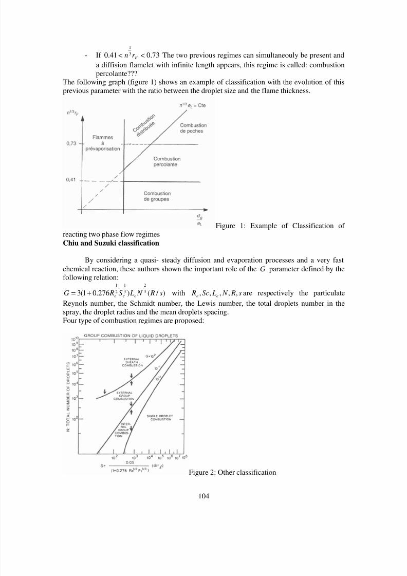
8/10/2019 Two phase flow in combustion system
http://slidepdf.com/reader/full/two-phase-flow-in-combustion-system 104/177
104
- If 73.041.0 3
1
<< F r n The two previous regimes can simultaneouly be present anda diffision flamelet with infinite length appears, this regime is called: combustionpercolante???
The following graph (figure 1) shows an example of classification with the evolution of thisprevious parameter with the ratio between the droplet size and the flame thickness.
Figure 1: Example of Classification ofreacting two phase flow regimesChiu and Suzuki classification
By considering a quasi- steady diffusion and evaporation processes and a very fastchemical reaction, these authors shown the important role of the G parameter defined by thefollowing relation:
) / ()276.01(3 3
2
3
1
2
1
s R N LS RGece+= with s R N LSc R
ee ,,,,, are respectively the particulate
Reynols number, the Schmidt number, the Lewis number, the total droplets number in thespray, the droplet radius and the mean droplets spacing.Four type of combustion regimes are proposed:
Figure 2: Other classification
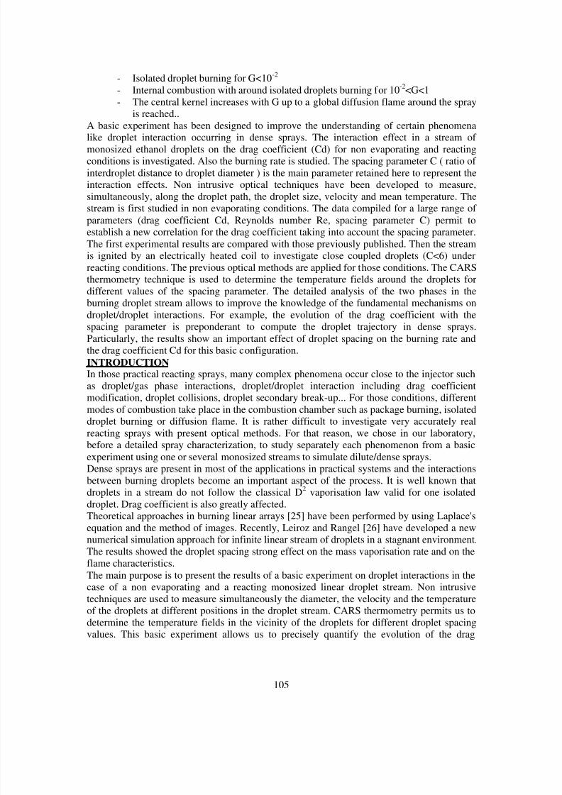
8/10/2019 Two phase flow in combustion system
http://slidepdf.com/reader/full/two-phase-flow-in-combustion-system 105/177
8/10/2019 Two phase flow in combustion system
http://slidepdf.com/reader/full/two-phase-flow-in-combustion-system 106/177
8/10/2019 Two phase flow in combustion system
http://slidepdf.com/reader/full/two-phase-flow-in-combustion-system 107/177
107
Droplet Size MeasurementsThe measurements of size and temperature of the droplets are based on the interactionsbetween a spherical droplet and a light ray [29,30]. In our case, a laser beam is focused alongthe axis of the droplet stream. The refracted rays of order 0 and 1 generate an interferencepattern in the forward direction. Because of the high droplets frequency production, astationary light pattern can be observed. The intensity distribution of the scattered light can be
described by the equations of Mie’s theory which introduces the dimensionless Mie parameter
απ
λ=
gD
where λ is the light wavelength. But for Mie parameter α >>1, equations of geometricaloptics can be used instead of the more complicated Mie theory to calculate the intensitydistribution of the scattered light. However, this simplification fails close to the forwarddirection and near the rainbow angle and thus is only valid for angles between 30° and 80°.As the droplets and the observation angle in the present experiment fulfill these conditions,the signal is recorded by a linear CCD array (camera 1, Fig.3). The angular spacing ismeasured between two interference maxima to calculate the droplet size. With this method,the determination of the droplet size is done with an accuracy of 2%.
Droplet Temperature MeasurementsFor refracted ray with order larger than one, the classical rainbow phenomena are observed inthe backward direction. However only the first rainbow created by the rays of order 2 isstrong enough to be easily detected. The classical optic laws explain that the position of therainbow is a function of the liquid refractive index and ray scattering order only. Therefractive index is a function of liquid density, thus of its temperature. For this reason thedroplet mean temperature can be determined by measuring the rainbow angle. The position ofthe first rainbow is recorded by another linear CCD array (camera 3, Fig.3).Determination of the refractive index of the droplet from the rainbow angle is done by meansof Airy/Walker theory. For this calculation method, the droplet diameter, the refractiveindex/temperature relationship and the angular position of the rainbow have to be known. Therefractive index/temperature relationship for ethanol (90 % purity) is obtained experimentally
using a refractometer at the wavelength of 632.8 nm (He-Ne laser). To obtain the angularposition, a mirror is located precisely at the focal point. The calibration is conducted byrotating the mirror to sweep the CCD array pixels with a laser beam.Droplet Velocity MeasurementsTo measure the droplet velocity, we use a second laser beam expanded as a laser sheet [31].This laser sheet is used to illuminate the droplet stream at the same location where the sizemeasurement is performed. Several droplets are present within the laser sheet at any giveninstant. The spacing between the droplets act as new point light sources. Young's fringes canbe observed in a perpendicular plane to the optical axis of the illumination. They are recordedby another CCD array (camera 2, Fig.3). By measuring the interfrange value, the dropletspacing is obtained and then the droplet velocity by means of the droplet productionfrequency. Such technique is only valid for monodispersed droplet linear streams. Howeverfor a droplet spacing greater than seven, the Young’s fringes method fails. In this case, avideo camera is used. The droplets are observed by shadowgraphy and their measured spacingis used to determine their velocity again.By simultaneously measuring the droplet size, velocity and temperature at different locationsdownstream from the injector, the temporal evolution of the liquid phase can be determinedeither with or without combustion.
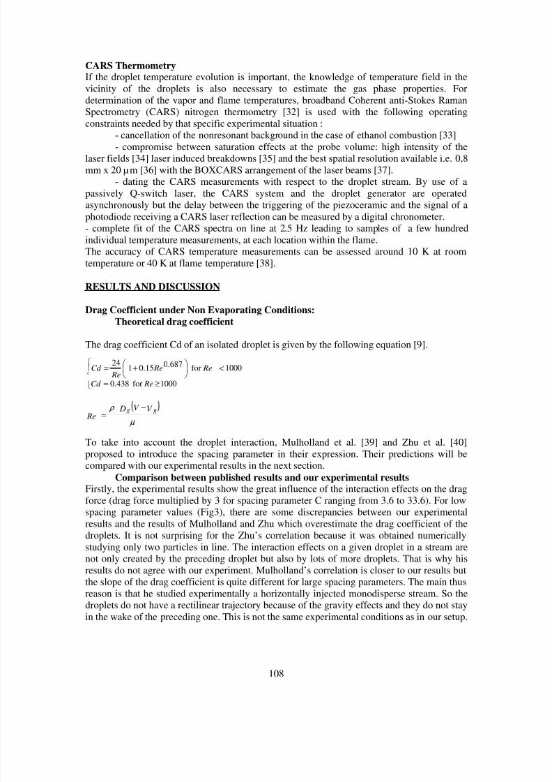
8/10/2019 Two phase flow in combustion system
http://slidepdf.com/reader/full/two-phase-flow-in-combustion-system 108/177
108
CARS ThermometryIf the droplet temperature evolution is important, the knowledge of temperature field in thevicinity of the droplets is also necessary to estimate the gas phase properties. Fordetermination of the vapor and flame temperatures, broadband Coherent anti-Stokes RamanSpectrometry (CARS) nitrogen thermometry [32] is used with the following operatingconstraints needed by that specific experimental situation :
- cancellation of the nonresonant background in the case of ethanol combustion [33]- compromise between saturation effects at the probe volume: high intensity of thelaser fields [34] laser induced breakdowns [35] and the best spatial resolution available i.e. 0,8mm x 20 µm [36] with the BOXCARS arrangement of the laser beams [37].
- dating the CARS measurements with respect to the droplet stream. By use of apassively Q-switch laser, the CARS system and the droplet generator are operatedasynchronously but the delay between the triggering of the piezoceramic and the signal of aphotodiode receiving a CARS laser reflection can be measured by a digital chronometer.- complete fit of the CARS spectra on line at 2.5 Hz leading to samples of a few hundredindividual temperature measurements, at each location within the flame.The accuracy of CARS temperature measurements can be assessed around 10 K at roomtemperature or 40 K at flame temperature [38].
RESULTS AND DISCUSSION
Drag Coefficient under Non Evaporating Conditions:Theoretical drag coefficient
The drag coefficient Cd of an isolated droplet is given by the following equation [9].
≥=
<
+=
1000for 0.438
1000for687.015.0124
ReCd
Re Re Re
Cd
µ ρ V V D Re gg −=
To take into account the droplet interaction, Mulholland et al. [39] and Zhu et al. [40]proposed to introduce the spacing parameter in their expression. Their predictions will becompared with our experimental results in the next section.
Comparison between published results and our experimental resultsFirstly, the experimental results show the great influence of the interaction effects on the dragforce (drag force multiplied by 3 for spacing parameter C ranging from 3.6 to 33.6). For lowspacing parameter values (Fig3), there are some discrepancies between our experimentalresults and the results of Mulholland and Zhu which overestimate the drag coefficient of thedroplets. It is not surprising for the Zhu’s correlation because it was obtained numerically
studying only two particles in line. The interaction effects on a given droplet in a stream arenot only created by the preceding droplet but also by lots of more droplets. That is why hisresults do not agree with our experiment. Mulholland’s correlation is closer to our results butthe slope of the drag coefficient is quite different for large spacing parameters. The main thusreason is that he studied experimentally a horizontally injected monodisperse stream. So thedroplets do not have a rectilinear trajectory because of the gravity effects and they do not stayin the wake of the preceding one. This is not the same experimental conditions as in our setup.
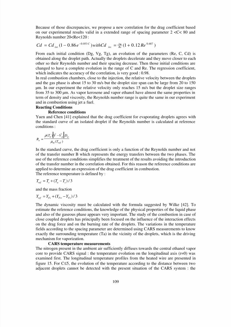
8/10/2019 Two phase flow in combustion system
http://slidepdf.com/reader/full/two-phase-flow-in-combustion-system 109/177
109
Because of those discrepancies, we propose a new correlation for the drag coefficient basedon our experimental results valid in a extended range of spacing parameter 2 <C< 80 andReynolds number 20<Re<120 :
)12.01()86.01( 687.024053.0 RewithCd eCd Cd
Reiso
C
iso +=−= −
From each initial condition (Dg, Vg, Tg), an evolution of the parameters (Re, C, Cd) is
obtained along the droplet path. Actually the droplets decelerate and they move closer to eachother so their Reynolds number and their spacing decrease. Then those initial conditions arechanged to have a complete evolution in the range of C and Re. The regression coefficient,which indicates the accuracy of the correlation, is very good : 0.98.In real combustion chambers, close to the injection, the relative velocity between the dropletsand the gas phase is about 15 to 30 m/s but the droplet size span can be large from 20 to 150µm. In our experiment the relative velocity only reaches 15 m/s but the droplet size rangesfrom 35 to 300 µm. As vapor kerosene and vapor ethanol have almost the same properties interm of density and viscosity, the Reynolds number range is quite the same in our experimentand in combustion using jet a fuel.Reacting Conditions
Reference conditionsYuen and Chen [41] explained that the drag coefficient for evaporating droplets agrees withthe standard curve of an isolated droplet if the Reynolds number is calculated at referenceconditions :
RT V V D
T e
a g g
m ref
=− ρ
µ
( )
( )
r r
In the standard curve, the drag coefficient is only a function of the Reynolds number and notof the transfer number B which represents the energy transfers between the two phases. Theuse of the reference conditions simplifies the treatment of the results avoiding the introductionof the transfer number in the correlation obtained. For this reason the reference conditions areapplied to determine an expression of the drag coefficient in combustion.The reference temperature is defined by :
T T T T ref s a s
= + −( ) / 3
and the mass fraction
Y Y Y Y ref Fs F Fs= + −∞( ) / 3
The dynamic viscosity must be calculated with the formula suggested by Wilke [42]. Toestimate the reference conditions, the knowledge of the physical properties of the liquid phaseand also of the gaseous phase appears very important. The study of the combustion in case ofclose coupled droplets has principally been focused on the influence of the interaction effectson the drag force and on the burning rate of the droplets. The variations in the temperature
fields according to the spacing parameter are determined using CARS measurements to knowexactly the surrounding temperature (Ta) in the vicinity of the droplets, which is the drivingmechanism for vaporization.
CARS temperature measurementsThe nitrogen present in the ambient air sufficiently diffuses towards the central ethanol vaporcore to provide CARS signal : the temperature evolution on the longitudinal axis (r=0) wasexamined first. The longitudinal temperature profiles from the heated wire are presented infigure 15. For C≤5, the evolution of the temperature according to the distance between twoadjacent droplets cannot be detected with the present situation of the CARS system : the
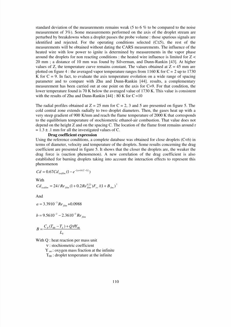
8/10/2019 Two phase flow in combustion system
http://slidepdf.com/reader/full/two-phase-flow-in-combustion-system 110/177
110
standard deviation of the measurements remains weak (5 to 6 % to be compared to the noisemeasurement of 3%). Some measurements performed on the axis of the droplet stream areperturbed by breakdowns when a droplet passes the probe volume : those spurious signals areidentified and rejected. For the operating conditions selected (C≤5), the rest of themeasurements will be obtained without dating the CARS measurements. The influence of theheated wire with low power to ignite is determined by measurements in the vapor phase
around the droplets for non reacting conditions : the heated wire influence is limited for Z <20 mm ; a distance of 10 mm was found by Silverman, and Dunn-Rankin [43]. At highervalues of Z, the temperature curve remains constant. The values obtained at Z = 45 mm areplotted on figure 4 : the averaged vapor temperature ranges from 1160 K for C = 2 up to 1730K for C = 9. In fact, to evaluate the axis temperature evolution on a wide range of spacingparameter and to compare with Zhu and Dunn-Rankin [44]. results, a complementarymeasurement has been carried out at one point on the axis for C=9. For that condition, thelower temperature found is 70 K below the averaged value of 1730 K. This value is consistentwith the results of Zhu and Dunn-Rankin [44] : 80 K for C =10
The radial profiles obtained at Z = 25 mm for C = 2, 3 and 5 are presented on figure 5. Thecold central zone extends radially to two droplet diameters. Then, the gases heat up with a
very steep gradient of 900 K/mm and reach the flame temperature of 2000 K that correspondsto the equilibrium temperature of stochiometric ethanol-air combustion. That value does notdepend on the height Z and on the spacing C. The location of the flame front remains around r= 1.3 ± .1 mm for all the investigated values of C.
Drag coefficient expressionUsing the reference conditions, a complete database was obtained for close droplets (C<6) interms of diameter, velocity and temperature of the droplets. Some results concerning the dragcoefficient are presented in figure 5. It shows that the closer the droplets are, the weaker thedrag force is (suction phenomenon). A new correlation of the drag coefficient is alsoestablished for burning droplets taking into account the interaction effects to represent thisphenomenon
)1(67.0)]1([ −+−
−= C ba
isofilm eCd Cd With
223.0 )1 /()2.01( / 24 fimev film filmisofilm BF Re ReCd ++=
And
film Rea
33910.3 −= +0.0988
25610.9 −=b film Re
33610.2 −−
V
S P
L
Y QT T C B
0000 )( ϑ +−=
With Q : heat reaction per mass unit ν : stochiometric coefficientY oo : oxygen mass fraction at the infiniteT00 : droplet temperature at the infinite
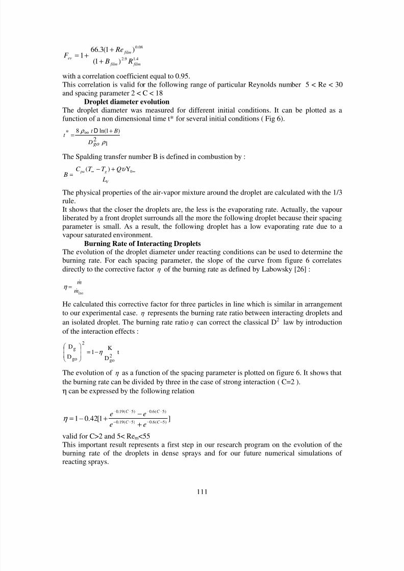
8/10/2019 Two phase flow in combustion system
http://slidepdf.com/reader/full/two-phase-flow-in-combustion-system 111/177
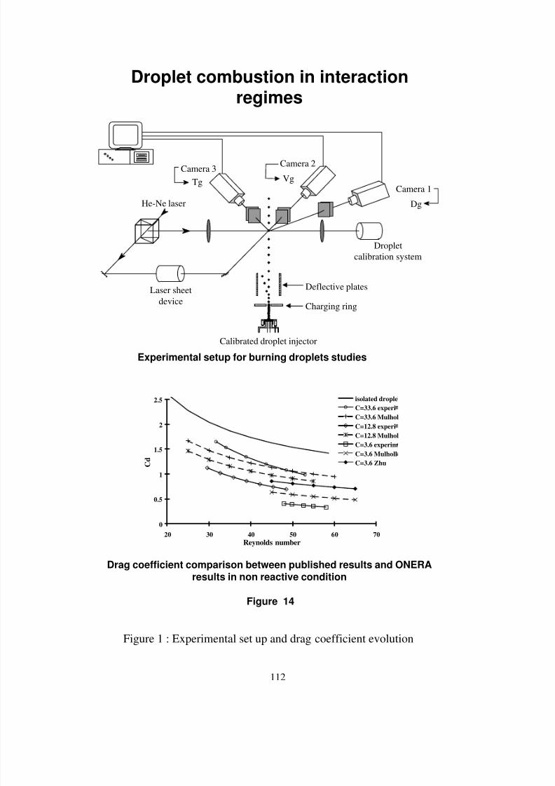
8/10/2019 Two phase flow in combustion system
http://slidepdf.com/reader/full/two-phase-flow-in-combustion-system 112/177
112
Figure 14
Droplet combustion in interactionregimes
Laser sheetdevice
He-Ne laser
Dropletcalibration system
Calibrated droplet injector
Camera 3
Camera 1
Dg
Camera 2
Charging ring
Deflective plates
Tg Vg
0
0.5
1
1.5
2
2.5
20 30 40 50 60 70Reynolds number
C d
isolated dropleC=33.6 experiC=33.6 MulholC=12.8 experiC=12.8 MulholC=3.6 experimC=3.6 MulhollC=3.6 Zhu
Experimental setup for burning droplets studies
Drag coefficient comparison between published results and ONERAresults in non reactive condition
Figure 1 : Experimental set up and drag coefficient evolution
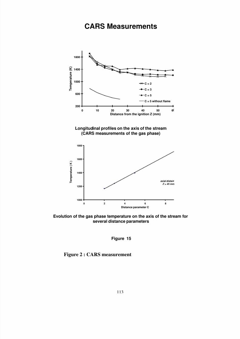
8/10/2019 Two phase flow in combustion system
http://slidepdf.com/reader/full/two-phase-flow-in-combustion-system 113/177
113
Figure 15
CARS Measurements
200
600
1000
1400
1800
0 10 20 30 40 50 6
Distance from the ignition Z (mm)
T e m p e r a t u r e ( K )
C = 2
C = 3
C = 5
C = 5 without flame
axial distan
Z = 45 mm
1000
1200
1400
1600
1800
0 2 4 6 8
Distance parameter C
T e m
p e r a t u r e ( K )
Evolution of the gas phase temperature on the axis of the stream forseveral distance parameters
Longitudinal profiles on the axis of the stream(CARS measurements of the gas phase)
Figure 2 : CARS measurement
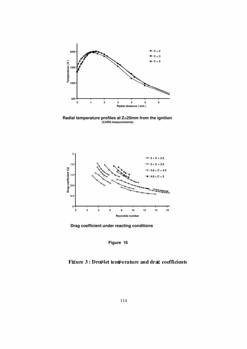
8/10/2019 Two phase flow in combustion system
http://slidepdf.com/reader/full/two-phase-flow-in-combustion-system 114/177
114
Figure 16
500
1000
1500
2000
0 1 2 3 4 5 6
Radial distance ( mm )
T e m p e r a t u r e ( K )
C = 2
C = 3
C = 5
Radial temperature profiles at Z=25mm from the ignition
(CARS measurements)
0
0.4
0.8
1.2
1.6
2
0 2 4 6 8 10 12 14 16
Reynolds number
D r a g c o
e f f i c i e n t C d
2 < C < 2.5
3 < C < 3.5
3.8 < C < 4.2
4.8 < C < 5
Drag coefficient under reacting conditions
Fi ure 3 : Dro let tem erature and dra coefficients
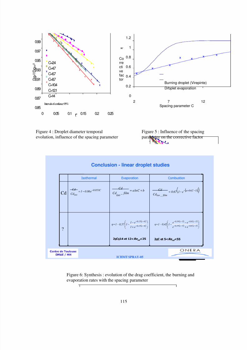
8/10/2019 Two phase flow in combustion system
http://slidepdf.com/reader/full/two-phase-flow-in-combustion-system 115/177
115
ICHMT SPRAY-05
Conclusion - linear droplet studies
CombustionEvaporationIsothermal
C 0530
iso
e86 01Cd
Cd .. −−= bC lna film_
isoCd
Cd += [ ])(
_. 1C ba
filmiso
e167 0Cd
Cd −+−−=
( )
( )
+
−−−=
−−
−−
6 c0,13
6 c0,13
e1
e110,57 1η
( ) ( )
( ) ( )
+
−−−=
−−−−
−−−−
5c0,6 5c0,19
5c0,6 5c0,19
ee
ee10,421η
2≤≤≤≤C≤≤≤≤14 et 12<Re ref
<25 2≤≤≤≤C et 5<Re ref
<55
?
Cd
0
0.2
0.4
0.6
0.8
1
1.2
2 7 12Spacing parameter C
Correctivefactor
Burning droplet (Virepinte)
Droplet evaporation
0.85
0.87
0.89
0.91
0.93
0.95
0.97
0.99
0 0.05 0.1 0.15 0.2 0.25t*
D g c ² / D g o c ² C=2.4
C=4.7
C=6.7
C=8.7
C=10.4
C=12.1
C=14
Intervals of confiance 95%
Figure 4 : Droplet diameter temporalevolution, influence of the spacing parameter
Figure 5 : Influence of the spacingparameter on the corrective factor
Figure 6: Synthesis : evolution of the drag coefficient, the burning andevaporation rates with the spacing parameter
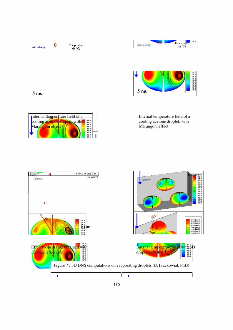
8/10/2019 Two phase flow in combustion system
http://slidepdf.com/reader/full/two-phase-flow-in-combustion-system 116/177
116
1 ms
Temperature(in °C)
Airvelocity
1 ms
Temperature(in °C)
Airvelocity
1 ms
Temperature(in °C)
Airvelocity
Air velocity θ Temperature
(in °C)
5 ms
Air velocity θ Temperature
(in °C)
5 ms
Air velocity θ Temperature
(in °C)
5 ms
0.1 ms
effective heat flux(in W/m²)
φ
θAirvelocity
0.1 ms
effective heat flux(in W/m²)
φ
θAirvelocity
0.1 ms
effective heat flux(in W/m²)
φ
θAirvelocity
Effective heat flux obtained with3D droplets cluster
Internal temperature field with 3Ddroplets cluster
Internal temperature field of acooling acetone droplet, withoutMarangoni effect
Air velocityTemperature
(in °C)
5 ms
θAir velocityTemperature
(in °C)
5 ms
θ
Internal temperature field of acooling acetone droplet, withMarangoni effect
Figure 7 : 3D DNS computations on evaporating droplets (B. Frackowiak PhD)
8/10/2019 Two phase flow in combustion system
http://slidepdf.com/reader/full/two-phase-flow-in-combustion-system 117/177
117
Chapter IX : Droplet wall interaction

8/10/2019 Two phase flow in combustion system
http://slidepdf.com/reader/full/two-phase-flow-in-combustion-system 118/177
118
The important amount of mass flow rate on the walls of the combustion chamber needs fueldroplet wall interaction modelling. All the different regimes characterising the droplet wallinteraction cannot be analyse in this lecture. We will focus on the rebound regime of a colddroplet on a heated wall.
DROPLET BEHAVIOR ON A HOT WALL
/wall temperature
Classification of the transfer regimes
Tb : liquid boiling temperature, Tp,c : Nukiyama temperature (1936) : intense thermalexchanges, Tp,L maximum boiling temperature: Leidenfrost temperature, presence of a vaporfilm between the hot wall and the liquid film. The thermal transfer is low in this case.
Lean evaporation regime (Tp<Tb) : the droplet is in contact with the wall (conduction flux)
Boiling regime (Tb<Tp<Tp,c) : formation of bubbles (vapor) at the center of the droplet
Transition regime(Tp,c<Tp< Tp,L ) : the droplet breaks up and many small droplets (orsatellites) are created.
Spheroîdal evaporation regime (Tp,L<Tp) : a vapor film is created between the wall andthe liquid film.
Regimes of thermal transfer between an ethanol droplet and inox wall
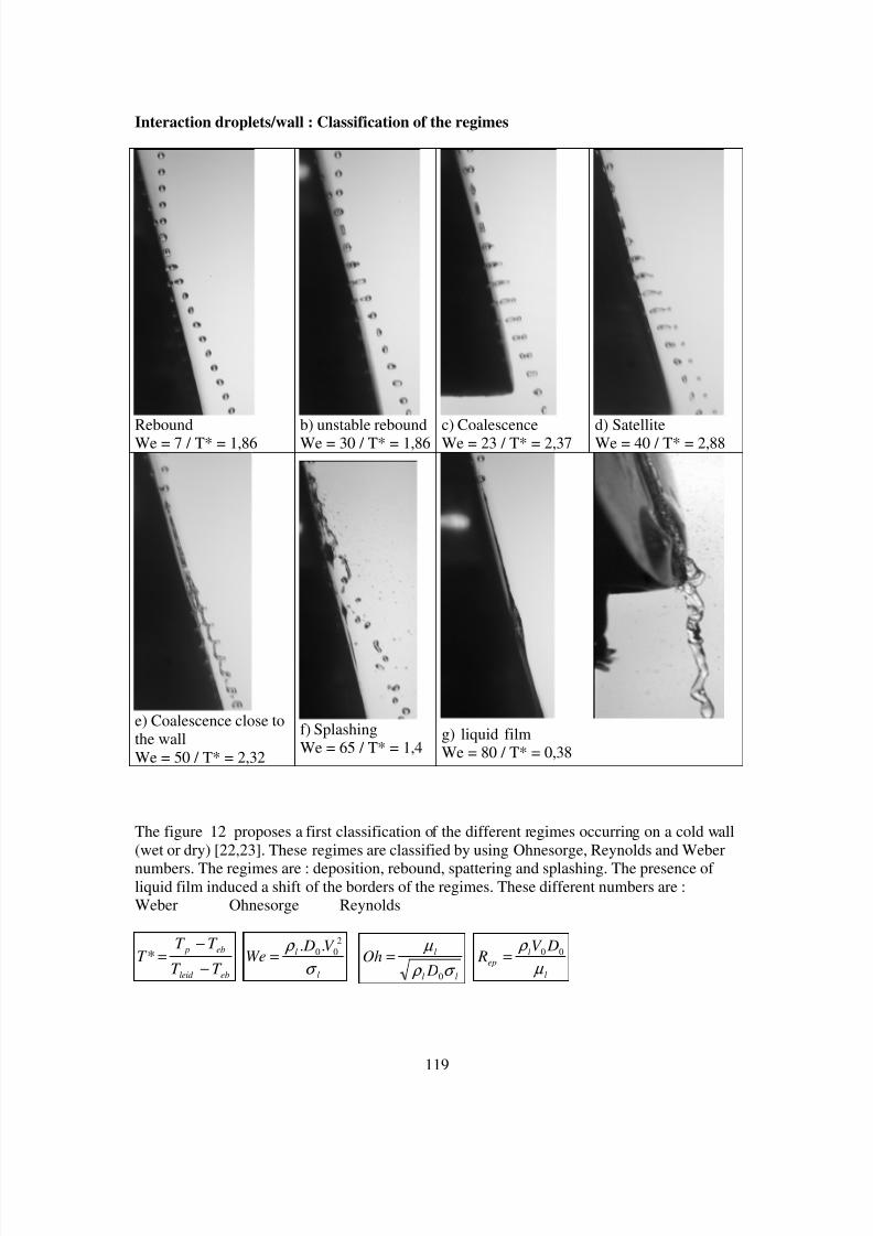
8/10/2019 Two phase flow in combustion system
http://slidepdf.com/reader/full/two-phase-flow-in-combustion-system 119/177
119
Interaction droplets/wall : Classification of the regimes
ReboundWe = 7 / T* = 1,86 b) unstable reboundWe = 30 / T* = 1,86 c) CoalescenceWe = 23 / T* = 2,37 d) SatelliteWe = 40 / T* = 2,88
e) Coalescence close tothe wallWe = 50 / T* = 2,32
f) SplashingWe = 65 / T* = 1,4
g) liquid filmWe = 80 / T* = 0,38
The figure 12 proposes a first classification of the different regimes occurring on a cold wall(wet or dry) [22,23]. These regimes are classified by using Ohnesorge, Reynolds and Weber
numbers. The regimes are : deposition, rebound, spattering and splashing. The presence ofliquid film induced a shift of the borders of the regimes. These different numbers are :Weber Ohnesorge Reynolds
ebleid
eb p
T T
T T T
−
−=*
l
l V D
Weσ
ρ 200 ..
= ll
l
DOh
σ ρ
µ
0
= l
l
ep
DV R
µ
ρ 00=

8/10/2019 Two phase flow in combustion system
http://slidepdf.com/reader/full/two-phase-flow-in-combustion-system 120/177
120
Tp: wall temperature, Teb: boiling temperature, TLeid: Leidenfrost temperature, D0: dropletdiameter, V0: droplet velocity, ρl: liquid density, µl: dynamic viscosity of the liquid, σl:surface tension of the liquid
Rebound regime of a cold droplet on a heated wall.If we analyse the evolution with wall temperature of the evaporation delay of a droplet located
on a hot plate, we can observe different regimes and particularly the Leidenfrost phenomenawhich occurs when a vapour film appears between the droplet and the hot wall.Experimental works developed in ONERA TOULOUSE (figure 13) around basic experimentsusing monosized droplets have permitted to elaborate a rebound model valid for theLeidenfrost regime (it is often the case in combustion chamber).
2maxmaxmax
)1(16imp
imp
imp
imp
reb
reb
We
We
We
We
We
We−=
Where impWe is the Weber number before impact σ ρ / 2 DpU Weinlimp
=
And inU is the normal incident droplet velocity, σ the surface tension of the liquid.
rebWe is the Weber number after the rebound defined by :
σ ρ / 2 DpU Wereblreb
= with rebU is the normal droplet velocity after the rebound.
maximp
We is a function of the droplet diameter and is given by P D
imp eWe
005.0max 368 −=
maxreb
We is constant = 3.5
The rebound angle is correlated by b
impreb aΘ=Θ , a and b are given by :
29.025.293510065
46.03.1440654168.076.475415.3
862.093.1855.3
==≤<≤
==≤<≤==≤<≤
==≤<
baand We
baand Webaand We
baand We
impimp
impmpi
impimp
impimp
θ
θ θ
θ
The heat exchange during droplet impact is given by the relation proposed by Deb and YAO[22] and is defined by ε which represents the ratio between real heat flux provide to thedroplet and heat flux necessary for a total droplet evaporation.
)1
90exp(
Pr21.0
)
5.60
(
)35
1(08.0exp027.0
5.1 iV
mpi
We
B
SF B
We Ln
+
−+
+
+=ε
withV
sW Pv
L
T T C B
)( −= 1−=
Pacacac
PW W W
C
C SF
ρ λ
ρ λ :PrV vapour Prandtl number
If the case of droplet deposition , Kendall and Rohsenow [24] expressed the diameter of theliquid disc created at the impact in function of droplet diameter and the Weber number beforeimpact.

8/10/2019 Two phase flow in combustion system
http://slidepdf.com/reader/full/two-phase-flow-in-combustion-system 121/177
121
)])12(
236arccos(
3
1cos[
18
125.1
imp
imp
filmWe
We Dp D
+
−+=
Clapeyron relation between the pressure of the saturated vapor and the boilingtemperature
( ) ( )2
lnlnT
D.PT C.
T
B AP
vp
ebvp +++=
where A, B, C et D are constants depending of the working liquid. For isooctane, the valuesare the following:
A = 58,265B = -6039,34C = -5,988
D = 6,48
350
400
450
500
550
0 5 10 15 20 25 30
P (bar)
T(K
Boiling temperature
Leidenfrost temperature
Leidenfrost and boiling temperature evolutions with the pressure

8/10/2019 Two phase flow in combustion system
http://slidepdf.com/reader/full/two-phase-flow-in-combustion-system 122/177
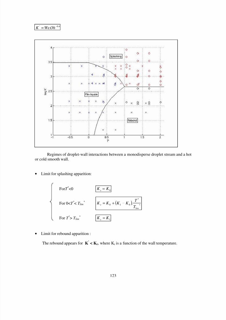
8/10/2019 Two phase flow in combustion system
http://slidepdf.com/reader/full/two-phase-flow-in-combustion-system 123/177
123
4.0' . −= OhWeK
Regimes of droplet-wall interactions between a monodisperse droplet stream and a hotor cold smooth wall.
• Limit for splashing apparition:
ForT *<0 0K K
s =
For 0<T *< T lim
* ( )*
lim
*
010 .T
T K K K K s −+=
For T *> T lim
* 1K K s =
• Limit for rebound apparition :
The rebound appears for K’ < Kr, where Kr is a function of the wall temperature.

8/10/2019 Two phase flow in combustion system
http://slidepdf.com/reader/full/two-phase-flow-in-combustion-system 124/177
124
ForT *<0 2K K r =
For 0<T *<T lim
*
=
2
*lim
*
12 .;maxT
T K K K r
For T *
> T lim*
1K K r = The values of the different constants are the following: :
K 0 = 3000K 1 = 450K 2 = 10T lim
* = 1
The validity of this classification is in the following range for T:* -0.6 <T
* < 2, and for
K’ 1 < log(K’) < 4.
The paper in annex presents more details of the modeling of the different regimes.
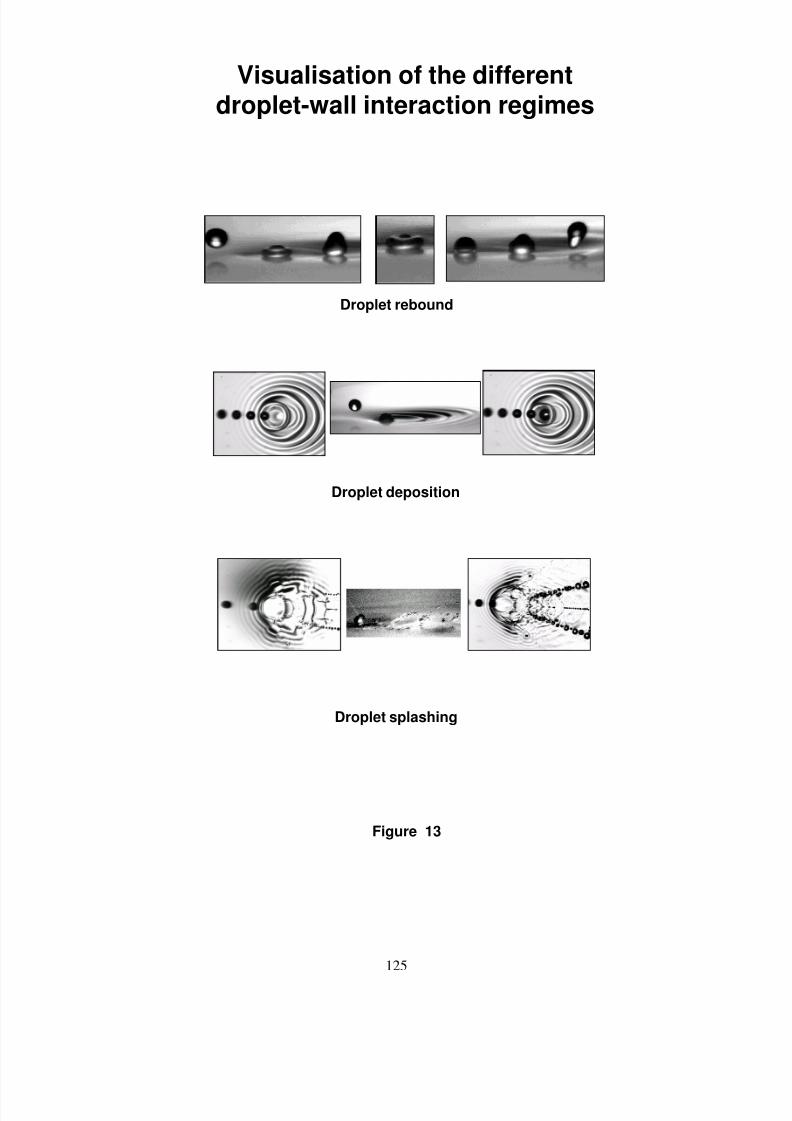
8/10/2019 Two phase flow in combustion system
http://slidepdf.com/reader/full/two-phase-flow-in-combustion-system 125/177

8/10/2019 Two phase flow in combustion system
http://slidepdf.com/reader/full/two-phase-flow-in-combustion-system 126/177
126
Chapter IX: Euler-Lagrange approach,Two Way coupling
8/10/2019 Two phase flow in combustion system
http://slidepdf.com/reader/full/two-phase-flow-in-combustion-system 127/177
127
In general, there are three different approaches in SF analyses for evaporating and combustingsprays :
- The "Particle-Source-in-Cell Model (PSICM), or Discrete-Droplet Model (DDM)uses a finite number of groups of particles to represent the entire spray. The motionand transport of representative samples of discrete drops are tracked through the
flow field using a Lagrangian simulation while a Eulerian formulation is used tosolve the governing equations for the gas-phase. The effect of droplets on the gasphase is taken into account by introducing appropriate source terms in the gasphase conservation equations. These source terms are derived by the use of dropletgasification models, which describe the evaporation or combustion of a singlealong its trajectory.
- The "Continuous Droplet Model (CDM) uses a distribution function f i (x,r,v,t) toevaluate the statistical distributions of the drop temperature, concentration, and soon. The transport equation for fj is solved along with the gas conservationequations to provide all properties of the spray. Similarly to the DDM, thegoverning equations for the gas phase must also included appropriate source terms.
- The "Continuum-Formulation Model (CFM) treats the motion of both drops andgas as though they are interpenetrating continua. A continuum formulation of theconservation equations for both phases is used to model spray combustion andevaporation problems. In this approach, the governing equations for the two phasesare similar. The first problem to be solved for the writing of these equations is tochose the quantities for characterising the spray. A first possibility is to considerthe spray as a single phase medium, which only a single (mean) velocity, a single(mean) temperature; this is the framework of the so-called "locally homogeneousspray" (LHS) introduced by G. FAETH and co-workers [1, 2, 3, 4]. But now asecond possibility is more often considered, with models that distinguish thetemperature and velocity of the gas phase and the ones of the liquid phase; theEulerian-Eulerian approach defines only a single (mean) temperature or velocityfor the liquid phase, and the Lagrangian-Eulerian models are able to distinguishone temperature or velocity for each droplet. Anyway, the equations have tocontain models in order to represent the small scale random phenomena, and thisconstitutes the second modelling problem. The problem is due to the fact that thequantities to be calculated by Eulerian equations are averaged quantities : theaverage is taken statistically in theory, or spatially and temporally in practice. Inthis approach, the governing equations for the two phases are similar; however,there are many difficulties in describing the droplet heat up process, the turbulentstresses, the turbulent dispersion of droplets, the droplet-wall interaction, thedroplet break up….Actually, the modelling of the combustion of sprays is still ininfancy. However some physical processes are now well known, the objective ofthis first lecture is to present the state of the art of some elementary phenomenalinked to the dispersed phase. The second lecture will be devoted to thepresentation of the Eulerian/Lagrangian approach and its applications tocombustion chambers of turbojet, ramjet and rocket.

8/10/2019 Two phase flow in combustion system
http://slidepdf.com/reader/full/two-phase-flow-in-combustion-system 128/177
128
THE PARTICLE SOURCE IN CELL MODEL (PSICM) FOR GAS DROPLETFLOWS
The primary problem in analysing a gas droplet flow suspension lies in treating the couplingof mass, momentum and energy between phases. These coupling phenomena comprise a verycomplex interaction which affects both the gas and droplet phases. Consider, for example,
cold non evaporative droplets in a hot gas flow. Heat is transferred from the gas to thedroplets convectively and there is a corresponding temperature decrease in the gas. Thedecreased gas temperature can alter the density in the gas flow field, which in turn maychange the gas flow field, the droplets trajectories and the heat transfer rate between thedroplets and the gas. The real problem is the introduction of all three sources terms in gasdroplet interaction.
Crowe, Sharama and Stock review [5] different approaches for the way coupling between gasand liquid phases. Furthermore, they present a two dimensional gas droplet flow model whichaccounts for all three modes of gas droplet coupling. This model is used within the presentstudy of turbulent reactive two phase flows. It is founded on the idea of treating droplets assource of mass, momentum and energy to the gaseous phase and hence is known as particle
source in cell model. The following sections describe the basic features of this model,including a short review of the gas phase equations and the droplet phase calculation. Explicitexpressions for the droplet source terms, providing the two way coupling between phases, aregiven also. Different applications of this approach will be presented at the end of this chapter.
BASIC CONCEPTIn order to apply the PSI-CELL model , it is first necessary to sub divide the flow field into aseries of cells. Such a subdivision is provided by the employed finite volume formulation ofthe gas phase governing equations.
As droplets traverse a given cell in this flow field they may be (figure 1) :
− evaporating or condensing, resulting in a source (or sink) of gaseous mass to the fluid inthe cell.
− accelerating or decelerating, resulting in a momentum augmentation or defiency in thefluid in the cell in the direction of droplet motion.
− conducting heat or convecting enthalpy, resulting in a source (or sink) of thermal energyto the fluid in the cell.
− Impinging hot wall, resulting in a rebound, deposition or splashing.
Using this concept, the analysis of the considered two phase flows is based on the followingpoints :
− Finite volume equations for mass, momentum and energy conservation are written foreach cell, incorporating the contribution due to the condensed phase. In other words thecontinuum flow field is analysed employing the Eulerian approach. The entire flow fieldsolution is obtained by solving the system of algebraic equations constituting the finitevolume equations for each cell
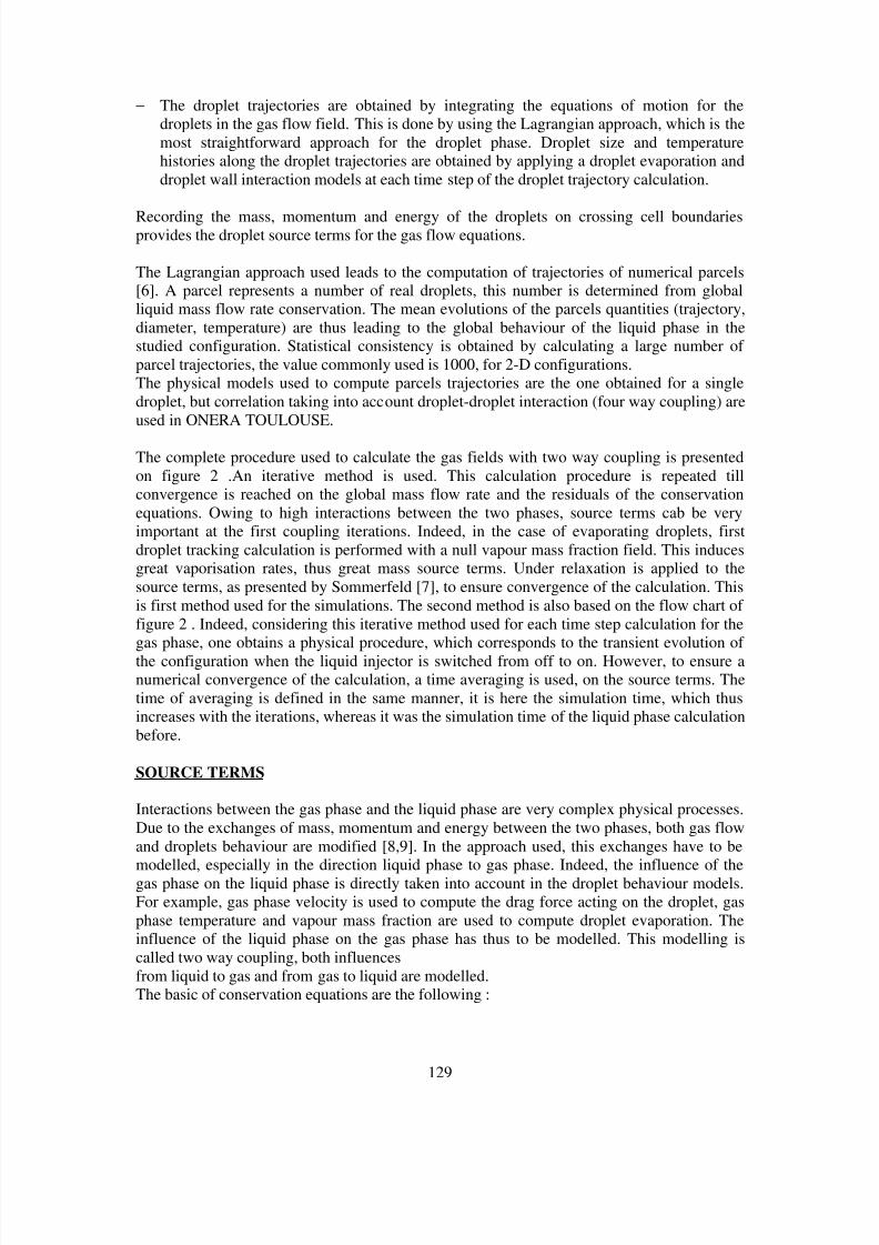
8/10/2019 Two phase flow in combustion system
http://slidepdf.com/reader/full/two-phase-flow-in-combustion-system 129/177
129
− The droplet trajectories are obtained by integrating the equations of motion for thedroplets in the gas flow field. This is done by using the Lagrangian approach, which is themost straightforward approach for the droplet phase. Droplet size and temperaturehistories along the droplet trajectories are obtained by applying a droplet evaporation anddroplet wall interaction models at each time step of the droplet trajectory calculation.
Recording the mass, momentum and energy of the droplets on crossing cell boundariesprovides the droplet source terms for the gas flow equations.
The Lagrangian approach used leads to the computation of trajectories of numerical parcels[6]. A parcel represents a number of real droplets, this number is determined from globalliquid mass flow rate conservation. The mean evolutions of the parcels quantities (trajectory,diameter, temperature) are thus leading to the global behaviour of the liquid phase in thestudied configuration. Statistical consistency is obtained by calculating a large number ofparcel trajectories, the value commonly used is 1000, for 2-D configurations.The physical models used to compute parcels trajectories are the one obtained for a singledroplet, but correlation taking into account droplet-droplet interaction (four way coupling) areused in ONERA TOULOUSE.
The complete procedure used to calculate the gas fields with two way coupling is presentedon figure 2 .An iterative method is used. This calculation procedure is repeated tillconvergence is reached on the global mass flow rate and the residuals of the conservationequations. Owing to high interactions between the two phases, source terms cab be veryimportant at the first coupling iterations. Indeed, in the case of evaporating droplets, firstdroplet tracking calculation is performed with a null vapour mass fraction field. This inducesgreat vaporisation rates, thus great mass source terms. Under relaxation is applied to thesource terms, as presented by Sommerfeld [7], to ensure convergence of the calculation. Thisis first method used for the simulations. The second method is also based on the flow chart offigure 2 . Indeed, considering this iterative method used for each time step calculation for thegas phase, one obtains a physical procedure, which corresponds to the transient evolution ofthe configuration when the liquid injector is switched from off to on. However, to ensure anumerical convergence of the calculation, a time averaging is used, on the source terms. Thetime of averaging is defined in the same manner, it is here the simulation time, which thusincreases with the iterations, whereas it was the simulation time of the liquid phase calculationbefore.
SOURCE TERMS
Interactions between the gas phase and the liquid phase are very complex physical processes.Due to the exchanges of mass, momentum and energy between the two phases, both gas flowand droplets behaviour are modified [8,9]. In the approach used, this exchanges have to be
modelled, especially in the direction liquid phase to gas phase. Indeed, the influence of thegas phase on the liquid phase is directly taken into account in the droplet behaviour models.For example, gas phase velocity is used to compute the drag force acting on the droplet, gasphase temperature and vapour mass fraction are used to compute droplet evaporation. Theinfluence of the liquid phase on the gas phase has thus to be modelled. This modelling iscalled two way coupling, both influencesfrom liquid to gas and from gas to liquid are modelled.The basic of conservation equations are the following :
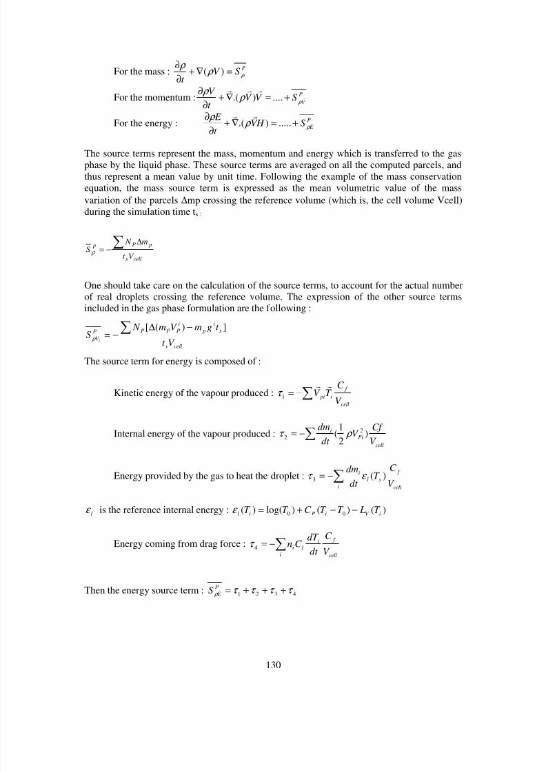
8/10/2019 Two phase flow in combustion system
http://slidepdf.com/reader/full/two-phase-flow-in-combustion-system 130/177
130
For the mass : PS V t
ρ ρ ρ
=∇+∂
∂)(
For the momentum : P
V S V V
t
V r
rrr
ρ ρ
ρ +=∇+
∂
∂....).(
For the energy : P
E S H V
t
E ρ ρ
ρ +=∇+
∂
∂.....).(
rr
The source terms represent the mass, momentum and energy which is transferred to the gasphase by the liquid phase. These source terms are averaged on all the computed parcels, andthus represent a mean value by unit time. Following the example of the mass conservationequation, the mass source term is expressed as the mean volumetric value of the massvariation of the parcels ∆mp crossing the reference volume (which is, the cell volume Vcell)during the simulation time ts :
cells
pPP
V t
m N S
∑ ∆−= ρ
One should take care on the calculation of the source terms, to account for the actual numberof real droplets crossing the reference volume. The expression of the other source termsincluded in the gas phase formulation are the following :
cells
s
i
p
i
PPPP
V V t
t gmV m N S
i
∑ −∆−=
])([ ρ
The source term for energy is composed of :
Kinetic energy of the vapour produced :cell
f
i pi
V
C T V rr
∑−=1τ
Internal energy of the vapour produced :cell
Pi
i
V
Cf V
dt
dm)
2
1( 2
2 ρ τ ∑−=
Energy provided by the gas to heat the droplet :cell
f
sl
i
i
V
C T
dt
dm)(3 ε τ ∑−=
lε is the reference internal energy : )()()log()( 00 iV iPil
T LT T C T T −−+=ε
Energy coming from drag force :cell
f il
i
iV
C
dt dT C n∑−=4τ
Then the energy source term : 4321 τ τ τ τ ρ +++=P
E S

8/10/2019 Two phase flow in combustion system
http://slidepdf.com/reader/full/two-phase-flow-in-combustion-system 131/177
131
Figure 18
Two phase flow code structure
Secondarybreak-up
Auto-ignition
Two phase flow moduleLSD
Combustion
Droplet-dropletdroplet-wall
interaction
Turbulentdispersion
PrimaryAtomisation
Unsteady
droplet injection
Evaporation
Navier Stockes numerical codefor the gas phase.
S o ur c e
t er m s
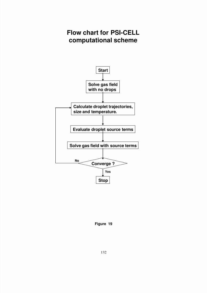
8/10/2019 Two phase flow in combustion system
http://slidepdf.com/reader/full/two-phase-flow-in-combustion-system 132/177
132
Figure 19
Flow chart for PSI-CELLcomputational scheme
Start
Solve gas fieldwith no drops
Calculate droplet trajectories,size and temperature.
Evaluate droplet source terms
Solve gas field with source terms
Stop
Converge ?
Yes
No
8/10/2019 Two phase flow in combustion system
http://slidepdf.com/reader/full/two-phase-flow-in-combustion-system 133/177
133
Chapter X : Examples of studiedconfigurations
8/10/2019 Two phase flow in combustion system
http://slidepdf.com/reader/full/two-phase-flow-in-combustion-system 134/177
134
Some examples of applications concerning airbreathing engines (ramjet and turbojet) androcket (booster of Ariane V) will be presented.DROPLET TRAJECTORY IN A TURBULENT FLOWThe drag coefficient correlation established for non-evaporating droplets was introduced inthe two phase CFD code LSD (Lagrangian Simulation of Droplets).The main features of the LSD code are:
Lagrangian transport
Gas velocity fluctuations taken in account for the dispersion
Droplet/gas phase interactions
Droplet/droplet interactions
Droplet/wall interactions
The gas phase simulation includes a k-ε model for the turbulence and a stochastic approach tobuild the instantaneous aerodynamic field. As test bench we have used an experimental set uplocated in our laboratory. A rectilinear monosized droplet stream was injected transversally ina cold flow. The experimental conditions were the following ones : Dg = 61 µm, Vg = 4.2m/s, f = 23000 droplets/second and air flow velocity Vair = 25 m/s. Figure 3 presents theexperimental visualizations realized on the experimental setup compared with twocomputations of the experiment: one using, for the motion equation of the droplets, the dragcorrelation of an isolated droplet and the other with our new correlation. The CFD codeapproach gives the overall spatial droplet dispersion by using the stochastic model. Only themean trajectory has been obtained from the experiment. The comparison underlines the goodagreement between our correlation and the experimental visualizations and also theimportance of the drag coefficient correlation to predict accurately the droplet trajectories
10]. Especially the droplet penetration into the turbulent flow is very sensitive to the dragcoefficient expression in this case.
DUMP COMBUSTOR [11]
A dump combustor is a very simplified geometry of ramjet. This simple geometrypermits to observe the main features of a real ramjet combustion chamber ; arecirculating zone and a jet zone.Concerning the liquid phase, kerosene droplets are injected in the dump. Five diameter groupsare used, 6 µ m, 18 µ m, 30 µ m, 50 µ m and 80 µ m. The injection is located at three injectionpoints, 45 mm before the expansion, and 3 mm, 4 mm and 5mm beneath the wall. Thus 15
parcel groups will be tracked.Droplet behaviour in the dump is shown on figure 4. A comparison between the flow fieldsobtained without two way coupling, and with two-way coupling (2 methods) is presentedfigures 4 and 5. One should first remark that the difference between the two coupling methodsare very small. However, the comparison of the computation times between the two methodsis in favour of the second one (simultaneous gas and liquid phase simulation).

8/10/2019 Two phase flow in combustion system
http://slidepdf.com/reader/full/two-phase-flow-in-combustion-system 135/177
135
LEAN PREMIXER PREVAPORISER MODULE [12]
The geometry is quite simple, a cylindrical part followed by a conic one,axisymetrical, but is representative of real modules. Current experimental studies conducted atONERA use the same kind of configuration, but swirl generators are added. These geometriesare also modelled.
The geometry of the module is shown of the figure 6. The inlet conditions, for the gas andliquid phases are the following :Velocity : smV / 95= ; pressure : bar P 9= ; temperature : K T 900= ; Fuel liquid : kerosene;injected equivalence ratio : 6.0=ϕ The initial conditions for the droplets were provided by PDPA measurements. The data wereprocessed, in order to obtain statistical results for five injection points, and five representativediameters for each point, this make 25 droplet groups. For each group, mean velocities as wellas fluctuating velocities were extracted from the velocity diameter correlation provided by thePDPA measurements.The aerodynamic field has been calculated with the MSD code (ONERA), on a 2D curvilinear116 /25 grid.The configuration is characterised by a higher air momentum in the module. In this case, one
should take into account droplet secondary break up, because the critical Weber number isreached for some drops in the module. However, for this application, the model has not beenintegrated in the coupled two phase flow numerical code. Now, collision and break up modelsare introduced in the new versions of the code.It appeared interesting to simulate this configuration, in order to test the 2-way couplingmodelling in a realistic case. The figure 6 shows also the evolution of the mass flow rate inthe inlet and outlet sections of the module for the 3 under relaxation values. The figure 6shows also, for three sections, the evolution of temperature discrepancy between one way andtwo way coupling. We can notice on the wall a temperature difference of 150K. A comparisonof fuel mass fraction profiles, with and without 2 way coupling are plotted on figure 7, forthree sections, from the injection section to the outlet section. The global evaporation rateleads to a mean value of about 0.18. With secondary break up modelling, the globalevaporation rate has been found to increase drastically to a value of about 100%. This lastresult means that the break up and wall film have to be modelled to ensure a good accuracy ofthe results.The coupling effect of the two phases is more effective on the evolution of the air temperatureprofiles. The mean temperature value in the module is about 490 K without 2-way coupling.Another operating conditions leading to ignition in the prevaporizer module has beencalculated by using ignition and combustion models (figure 7 ).
MODELLING OF THE TWO PHASE FLOW IN SOLID ROCKET MOTORS [13,14]
The aluminium particles included in the propellants to improve performances generate a two
phase flow in the solid propellant combustion chamber which creates a slag in the submergednozzle. The slag is evaluated with the particle impingement on the wall and slag criterions.When these propellants burn, the aluminium powder melts to form agglomerates on thepropellant surface. These agglomerates are then ejected by the propellant combustion gasesand generate a two phase flow in the motor chamber. Some of those agglomerates deposit onthe submerged nozzle in form of aluminium or alumina. Long motors with segmented grainand submerged nozzle are known to produce slag. After the first tests driven on the Ariane Vboosters 2 tons of alumina were found which represent 3% of the mass of alumina formedduring the combustion.
8/10/2019 Two phase flow in combustion system
http://slidepdf.com/reader/full/two-phase-flow-in-combustion-system 136/177
136
The Lagrangian two phase flow was used to compute this flow. Complementary models wereused to take into account the droplet wall interaction such liquid film model. Appropriateddroplet drag coefficient was chosen for transport droplet modelling in the nozzle and also amodified d2 law was retains for aluminium droplet combustionThe continuous phase is constituted by the propellant combustion gases. The maincomponents are H2O, C02, C0, HCL. This flow is simulated solving the NS equations with
the ONERA code MSD. This 3D code uses a k-l turbulence model on a structured grid. Theflow is steady, non reactive, without aluminium but with an equivalent density. The meanvalues obtained are then used as an input to the turbulent dispersion program. Twoconfigurations were tested.The first one is a motor with a simplified sub-scale geometry with no submerged nozzle and asingle grain segment. The grid is curvilinear with 4914 points. The chamber pressure is 45bar, the temperature is 2500 K. The particles are injected with a 1m/s velocity and a sizedistribution centred on 120 µm. The gravity acceleration is 1g in the axial direction.The figure 8 shows a great influence of the particle dispersion to the particle size and theirinjection point. The aluminium combustion was observed all along the trajectories withuncompleted combustion for the biggest particles (figure 8).The second configuration is the full scale geometry with a submerged nozzle to observe the
slag generation in more realistic conditions. In order to predict the slag over a whole flight,the flight time was discretized in 5 time steps : 50s, 66s, 82s, 95s, 115s. Here we will presentonly results concerning t= 95s. The grid has 18000 points, the mean pressure is 49 bar and themean temperature 3400K. The particles are injected with a velocity normal to the wallbetween 1m/s and 5m/s. In the aft-end the recirculation zone traps some of the particles issuedfrom the end of the grain figure 9 . The figure 9 indicates where the droplet aluminiumcombustion and the droplet alumina break up occur. The aluminium combustion is locatednear the propellant grain.Droplet collision models and droplet break up model have been introduced in the two phaseflow module to compute the droplet collision probability in the full scale motor (figure 10).
In the future the researches will be oriented towards dense two phase flows. ONERA hasalready elaborated some models such prediction of the collision (figure 10) by using kineticapproach, different regimes of collision [14], break up, corrective factors for drag coefficient,evaporation rate and burning rate.
References[1] FAETH, G, M, Evaporation and combustion of spraysProgress in Energy and Combustion Science, 9, pp 1-76, 1983
[2] FAETH, G, M, Recent advances in modelling particle transport properties and dispersionin turbulent flowASME/JSME, Vol 2, pp 517-534, 1983
[3] FAETH, G, M, Spray atomization and combustion24th Aerospace Sciences Meeting, AIAA 86-0136, Reno, 1986
[4] FAETH, G, M, Mixing transport and combustion in spraysProgress in Energy and Combustion Sciences 13 : 293-345, 1987
[5] CROWE, C, T, SHARAMA, M, P, and STOCK, The Particle Source in CellASME, Journal of Heat Transfer, pp325-332, 1975.

8/10/2019 Two phase flow in combustion system
http://slidepdf.com/reader/full/two-phase-flow-in-combustion-system 137/177
137
[6] MEHRING, C, Numerische simulation der verdampfung und verbrennung von trofen inreagierenden turbulenten strömungenDiplomarbeit ITLR, Univ STUTTGART, ONERA, centre de TOULOUSE.
[7] KOHNEN, G, RUGER, M, and SOMMERFELD, M,
Convergence behaviour for numerical calculations by the Euler/Lagrange method for stronglycoupled phases.ASME Fluids Engineering Division Summer Meeting, vol 185, pp 191-202, 1994.
[8] BERLEMONT, A, GOUESBET, G, and GRANCHER, M, S, On the Lagrangiansimulation of turbulence influence on droplet evaporationInt Journal Heat Mass Transfer, 34 (11) : pp 2805-2812, 1991
[9] Bissieres, D., (1997) Modélisation du comportement de la phase liquide dans les chambresde combustion des statoréacteurs. Phd Thesis, Ecole Centrale Paris.
[10] ADAM O. Etude expérimentale du comportement des gouttes en régime d'interaction.
PhD Thesis ENSAE, 1997
[11] BISSIERES, D, LAVERGNE, G, Two phase flow simulation of a dump combustorunder realistic conditionsICLASS 97, SEOUL, 1997
[12] BISSIERES, D, LAVERGNE, G, TRICHET, P, A study of the two way couplingmodelling for the two phase flow simulation in a lean premixer prevaporizer moduleICLASS 97, SEOUL
[13] CESCO, N, Etude et modélisation de l’écoulement diphasique à l’intérieur despropulseurs à poudre.Doct 3ème cycle ENSAE, nov 1997
[14] HYLKEMA, J, Modélisation cinétique et simulation numérique d’un brouillard dense degouttes.Doct 3ème cycle, ENSAE, mars 1999
[15] ESTRADE, J, P, Etude de la collision de gouttesDoct 3ème cycle, ENSAE (décembre 1998)

8/10/2019 Two phase flow in combustion system
http://slidepdf.com/reader/full/two-phase-flow-in-combustion-system 138/177
138
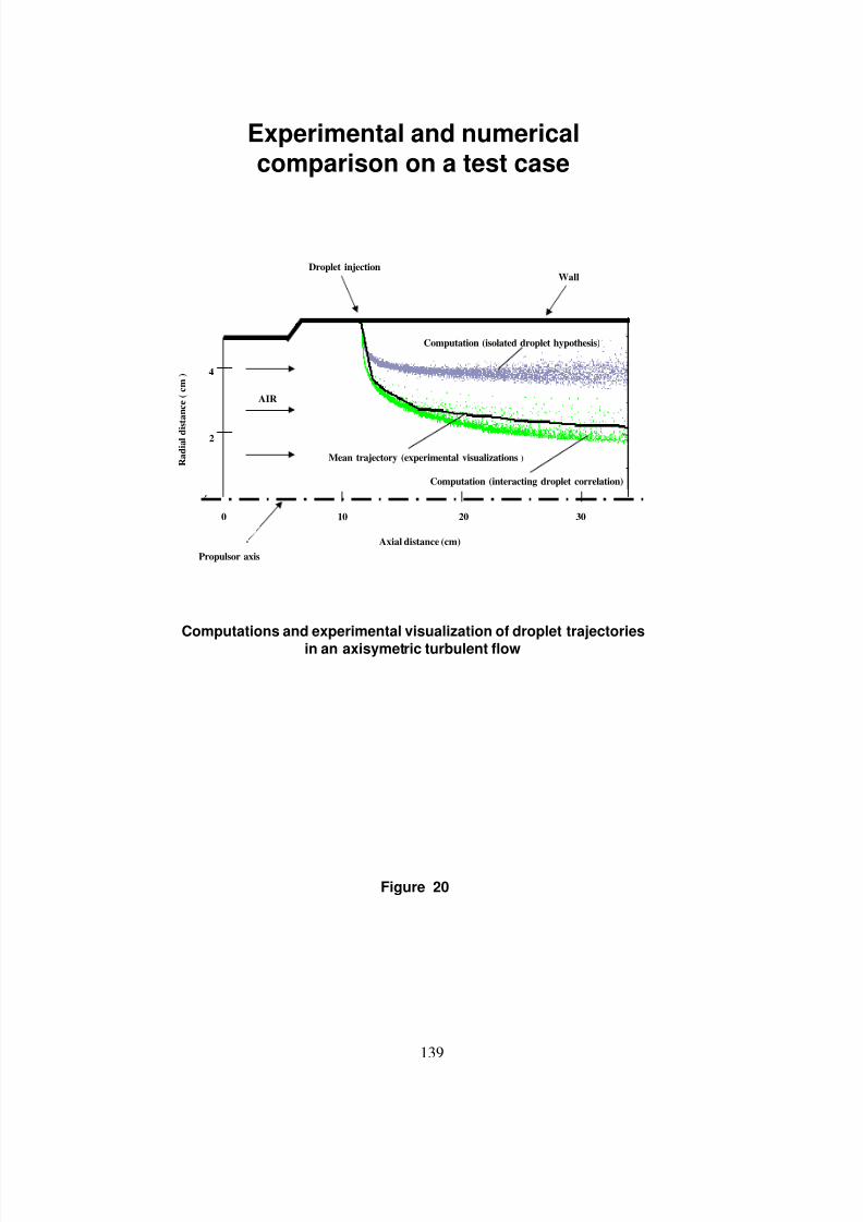
8/10/2019 Two phase flow in combustion system
http://slidepdf.com/reader/full/two-phase-flow-in-combustion-system 139/177
139
Figure 20
Experimental and numericalcomparison on a test case
40 50 7060
8
6
4
2
Propulsor axis
R a d i a l d i s t a n c e ( c m )
Computation (isolated droplet hypothesis)
Computation (interacting droplet correlation)
Mean trajectory (experimental visualizations)
Droplet injection
AIR
Wall
2
4
0 10 20 30
Axial distance (cm)
Computations and experimental visualization of droplet trajectoriesin an axisymetric turbulent flow
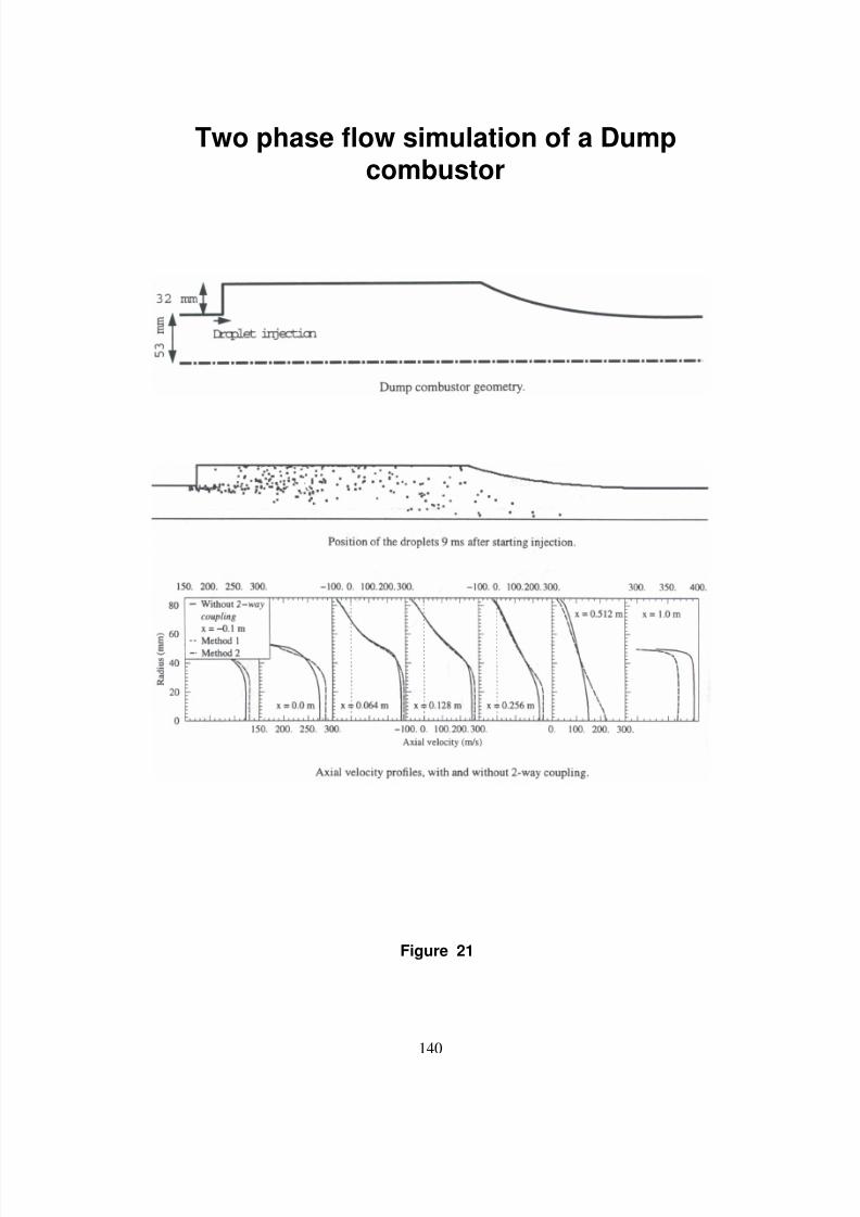
8/10/2019 Two phase flow in combustion system
http://slidepdf.com/reader/full/two-phase-flow-in-combustion-system 140/177
140
Figure 21
Two phase flow simulation of a Dumpcombustor
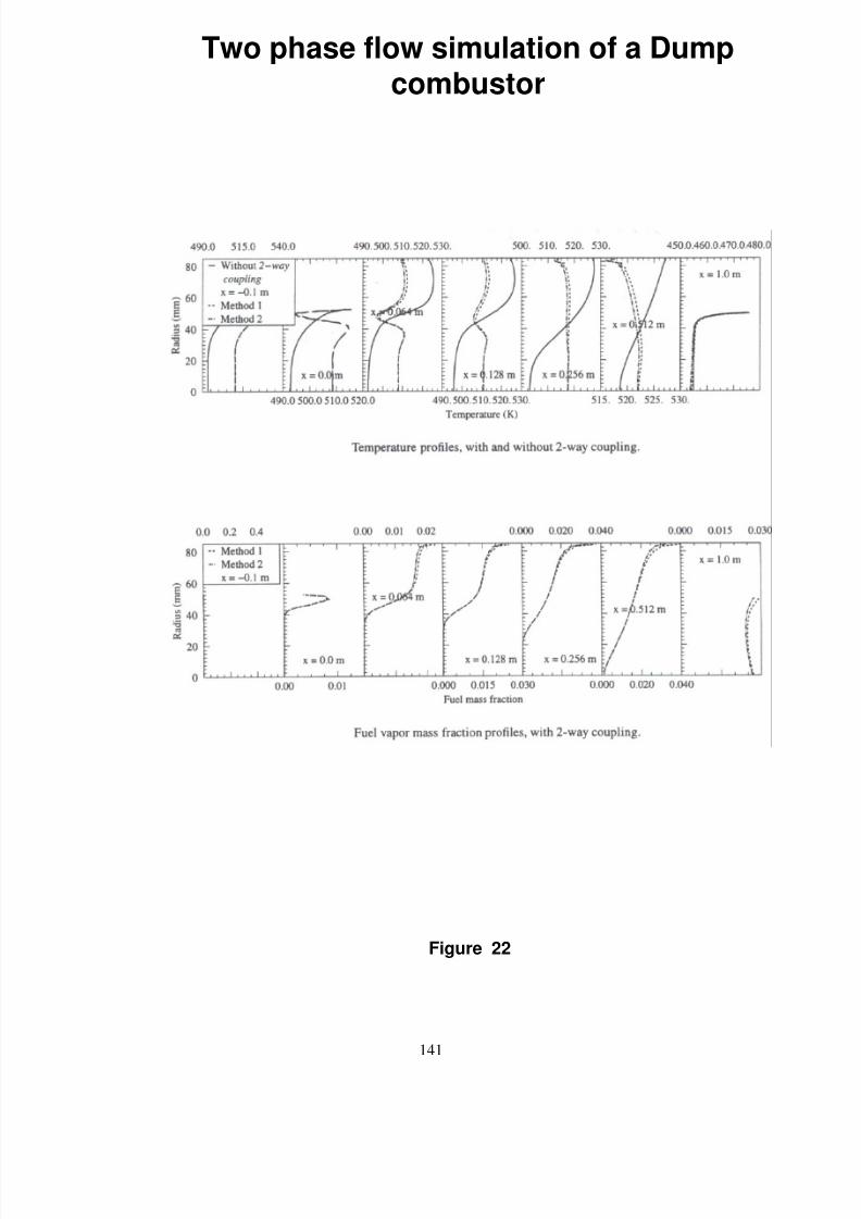
8/10/2019 Two phase flow in combustion system
http://slidepdf.com/reader/full/two-phase-flow-in-combustion-system 141/177
141
Figure 22
Two phase flow simulation of a Dumpcombustor

8/10/2019 Two phase flow in combustion system
http://slidepdf.com/reader/full/two-phase-flow-in-combustion-system 142/177
142

8/10/2019 Two phase flow in combustion system
http://slidepdf.com/reader/full/two-phase-flow-in-combustion-system 143/177
143
Figure 23
Two phase flow simulation ina LPP duct
Air
95 mm50 mm
23,3 mm
Airblast injector
15,5 mm
PDPA measurement plan
Air flow rate convergence
Temperature difference with and without two way coupling

8/10/2019 Two phase flow in combustion system
http://slidepdf.com/reader/full/two-phase-flow-in-combustion-system 144/177
144
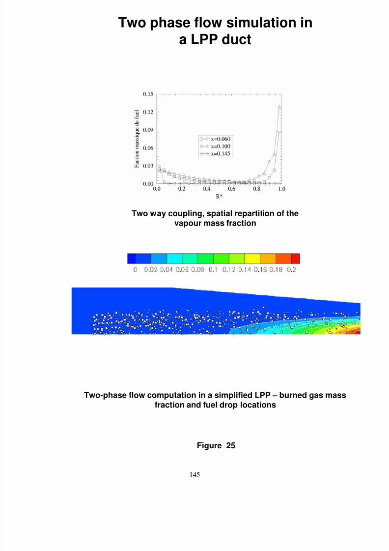
8/10/2019 Two phase flow in combustion system
http://slidepdf.com/reader/full/two-phase-flow-in-combustion-system 145/177
145
Figure 25
Two phase flow simulation ina LPP duct
Two-phase flow computation in a simplified LPP – burned gas massfraction and fuel drop locations
Two way coupling, spatial repartition of thevapour mass fraction
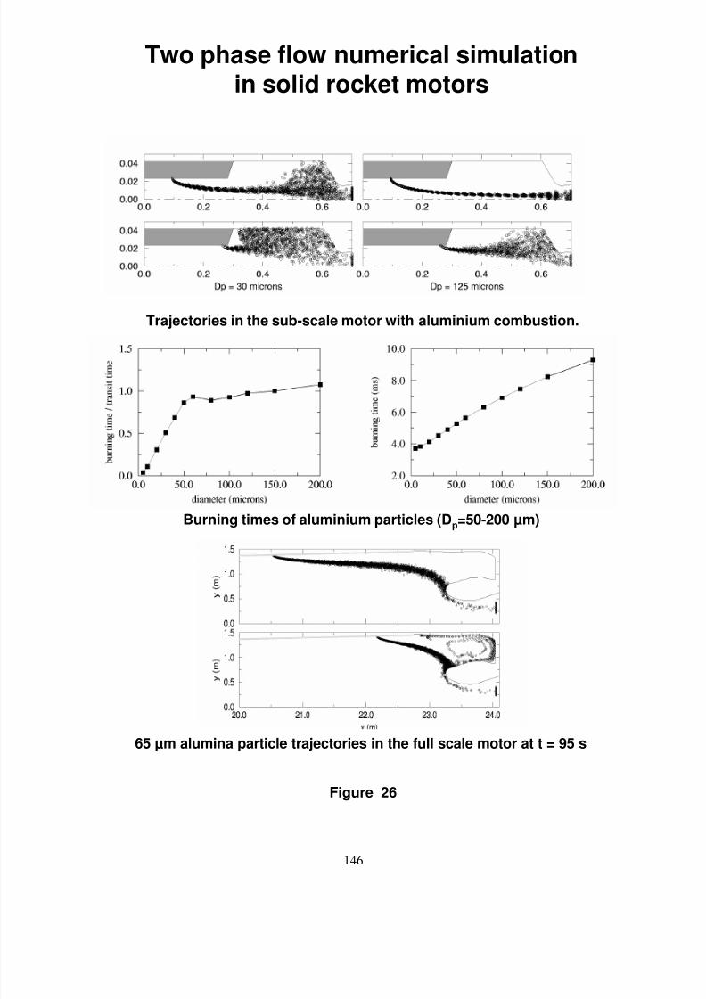
8/10/2019 Two phase flow in combustion system
http://slidepdf.com/reader/full/two-phase-flow-in-combustion-system 146/177
146
Figure 26
Two phase flow numerical simulationin solid rocket motors
Trajectories in the sub-scale motor with aluminium combustion.
Burning times of aluminium particles (Dp=50-200 µm)
65 µm alumina particle trajectories in the full scale motor at t = 95 s
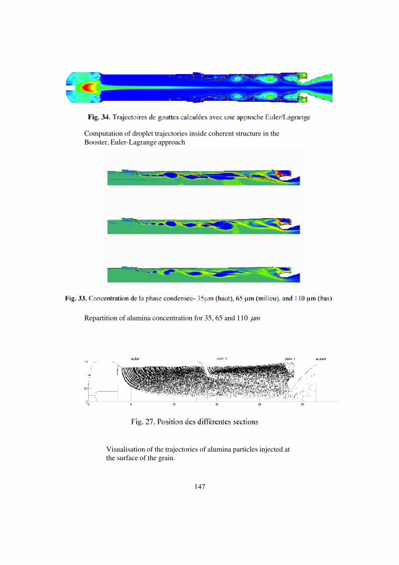
8/10/2019 Two phase flow in combustion system
http://slidepdf.com/reader/full/two-phase-flow-in-combustion-system 147/177
147
Computation of droplet trajectories inside coherent structure in theBooster, Euler-Lagrange approach
Repartition of alumina concentration for 35, 65 and 110 m µ
Visualisation of the trajectories of alumina particles injected atthe surface of the grain.
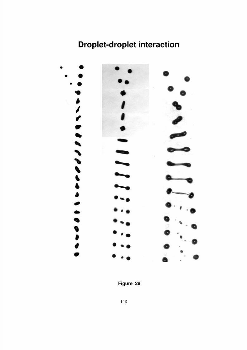
8/10/2019 Two phase flow in combustion system
http://slidepdf.com/reader/full/two-phase-flow-in-combustion-system 148/177
148
Figure 28
Droplet-droplet interaction

8/10/2019 Two phase flow in combustion system
http://slidepdf.com/reader/full/two-phase-flow-in-combustion-system 149/177
149
Superposition of aerodynamic axial velocity field and droplet
trajectories injected ::
(a) close to the chamber axis
(b) in the lateral recirculating zone
b in the lateral recirculation
3D Computation of a reactive two phase flow inside a real combustion chamber
Two phase flow modeling before ignition in a reactangular sector
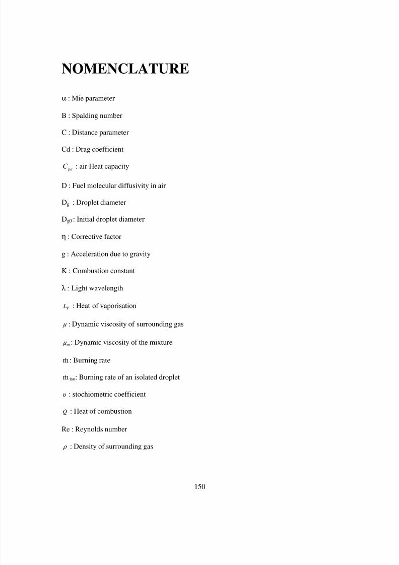
8/10/2019 Two phase flow in combustion system
http://slidepdf.com/reader/full/two-phase-flow-in-combustion-system 150/177
150
NOMENCLATURE
α : Mie parameter
B : Spalding number
C : Distance parameter
Cd : Drag coefficient
C pa : air Heat capacity
D : Fuel molecular diffusivity in air
Dg : Droplet diameter
Dg0 : Initial droplet diameter
η : Corrective factor
g : Acceleration due to gravity
K : Combustion constant
λ : Light wavelength
LV : Heat of vaporisation
µ : Dynamic viscosity of surrounding gas
µ m : Dynamic viscosity of the mixture
&m : Burning rate
&m iso: Burning rate of an isolated droplet
υ : stochiometric coefficient
Q : Heat of combustion
Re : Reynolds number
ρ : Density of surrounding gas
8/10/2019 Two phase flow in combustion system
http://slidepdf.com/reader/full/two-phase-flow-in-combustion-system 151/177
151
ρ m : Density of the mixture
l ρ : Liquid density
∞ ρ :gas density at infinite distance from the droplets
t : Time
t* : non dimensional time
aT : Temperature in the vicinity of the droplets
Tg : Droplet temperature
T ∞ : Room temperature
Tref : Reference temperature
sT : Droplet surface temperature
V : Velocity of surrounding gas
Vair : air flow velocity
FsY : Mass fraction at the droplet surface
∞F Y : Mass fraction of the free stream

8/10/2019 Two phase flow in combustion system
http://slidepdf.com/reader/full/two-phase-flow-in-combustion-system 152/177
152

8/10/2019 Two phase flow in combustion system
http://slidepdf.com/reader/full/two-phase-flow-in-combustion-system 153/177
153
ACKNOWLEDGEMENTSThe author acknowledges all the actual group of “Multiphase Flow” unit of ONERA centre deTOULOUSE for the scientific support. He would like also to thank all the PhD students thathave worked with me from 1978 in ONERA /Toulouse center.

8/10/2019 Two phase flow in combustion system
http://slidepdf.com/reader/full/two-phase-flow-in-combustion-system 154/177
154
Exercises
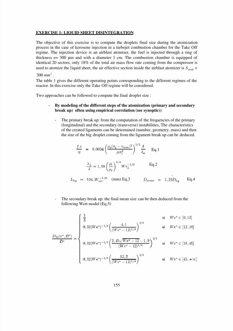
8/10/2019 Two phase flow in combustion system
http://slidepdf.com/reader/full/two-phase-flow-in-combustion-system 155/177
155
EXERCISE 1: LIQUID SHEET DISINTEGRATION
The objective of this exercise is to compute the droplets final size during the atomizationprocess in the case of kerosene injection in a turbojet combustion chamber for the Take Offregime. The injection device is an airblast atomiser, the fuel is injected through a ring of
thickness e= 300 µm and with a diameter 1 cm. The combustion chamber is equipped ofidentical 20 sectors, only 18% of the total air mass flow rate coming from the compressor isused to atomize the liquid sheet, the air effective section inside the airblast atomizer is aireff S =
300 2mm .
The table 1 gives the different operating points corresponding to the different regimes of thereactor. In this exercise only the Take Off regime will be considered.
Two approaches can be followed to compute the final droplet size :
- By modeling of the different steps of the atomization (primary and secondarybreak up) often using empirical correlation (see synoptic))
- The primary break up: from the computation of the frequencies of the primary(longitudinal) and the secondary (transverse) instabilities, The characteristicsof the created ligaments can be determined (number, geometry, mass) and thenthe size of the big droplet coming from the ligament break up can be deduced.
Eq.1
Eq.2
(mm) Eq.3 Eq.4
- The secondary break up: the final mean size can be then deduced from thefollowing Wert model (Eq.5)
8/10/2019 Two phase flow in combustion system
http://slidepdf.com/reader/full/two-phase-flow-in-combustion-system 156/177
156
- By using only one correlation linking the SMD (Sauter Mean Diameter) to themain parameters of the operating point (Lefebvre woks for example):
- 55.045.025.02 ) / (040,0) / (5,0)( jk lllg jk l d V d m DMS ρ σ µ σ +=
gV is the air velocity inside the atomizer, jk d corresponds in this case to the liquid
sheet thickness
Compare The final droplet mean size obtained by the two approaches, comments??
-Kerosene :
m N m NsmKglll / 0277,0, / 0013.0, / 827 23 === σ µ ρ
µ
ρ τ
18
2Pl
P
D= ,
Stoechiometric ratio (Air/Fuel)sto=15Liquid sheet thickness: =e m µ 300 ,
-Gas (Air)smv / 5.2min = , 17.061.4)( −= gvmmδ (boundary layer thickness)),
13.024.0)( −=gw
vmmδ (vorticity thickness)
paroig
lg
dy
dv
vv
.max.)(
−= ,
Weber number:l
lgg vvW
σ
δ ρ δ
2)( −= ,
l
lgg DvvW
σ
ρ *2**
*)( −
=
Ambient reference Pa p 50 10= , K T 2900 =
Designation :
= f frequency of the longitudinal instability
=λ wavelength of the transversal instability
=lig L ligament length
=amas
D amass diameter, =lig D ligament diameter
==air g
vv Air velocity outside the boundary layer
=lv liquid sheet velocity with (* reference to the amass)
l reference to the liquid
g reference to the gas (air)
Table 1
Take-Off Climb Out Approach Idle
OPR (-) 29.26 26.57 11.13 5
P3 (kPa) 2964.7 2672 1146.7 507
T3 (K) 844 801.9 617.4 509
W31 (kg/s) 45.39 42.6 21.8 10.6
WF (kg/s) 1.34 1.11 0.33 0.14
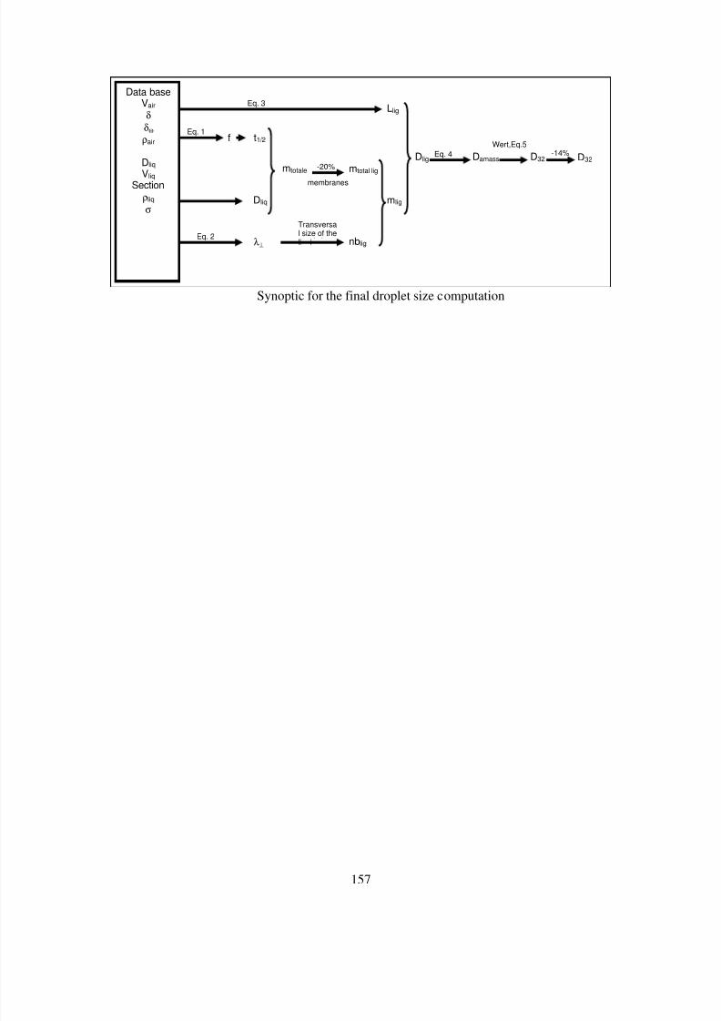
8/10/2019 Two phase flow in combustion system
http://slidepdf.com/reader/full/two-phase-flow-in-combustion-system 157/177
157
Synoptic for the final droplet size computation
Data baseVair
δ
δω
ρair
Dliq
VliqSectionρliq
σ
f t1/2Eq. 1
Dliq
mtotale-20%
membranes
mtotal lig
Eq. 2
Transversal size of theli iλ⊥ nblig
mlig
Eq. 3Llig
DligEq. 4 Damass
Wert,Eq.5
D32-14%
D32
8/10/2019 Two phase flow in combustion system
http://slidepdf.com/reader/full/two-phase-flow-in-combustion-system 158/177
158
EXERCISE 2: DROPLET EVAPORATION
The velocity of a turbojet is 160 m/s. If its length is 1.6 m and if the temperature inside thechamber is 1000 C, what is the maximum size of kerosene droplets injected in the chamberfor a total evaporation before the exit?
- By evaporation only
- By evaporation and combustion. In this case B will be computed from thefollowing expression :
L
T T C HfY B
Bg )(0 −+∆=
∞∞
The computation will be carried out by considering two values of the mass fraction ofoxygen :
Y ∞0 =23.2% et Y ∞0 =10%- Without convection and for hydrocarbons, a simple expression gives the ratiobetween the flame radius f r and the droplet radius gr
This expression is written :: )1(14 B Lnr
r
g
f += , compute this ratio.
What are the different regimes of combustion in a spray and what are the morepreponderant parameters influencing these regimes ?
Given data :
For air : C gcalC g / / 3.0= =)1000( C D
gg ρ 2 10-5Kg/M/s
For kerosene :
gcal H
f
gcal L
C T
mKg
B
l
/ 10300
316.0
/ 5.69
250
/ 825 3
=∆
=
=
=
= ρ
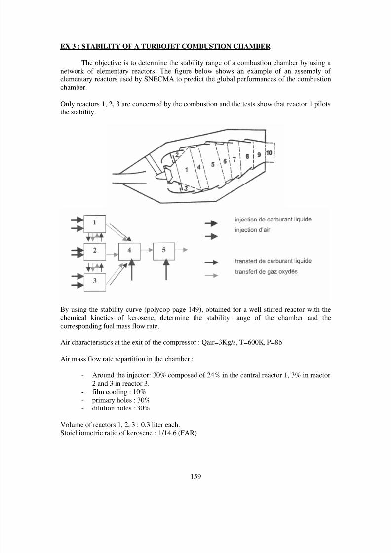
8/10/2019 Two phase flow in combustion system
http://slidepdf.com/reader/full/two-phase-flow-in-combustion-system 159/177
159
EX 3 : STABILITY OF A TURBOJET COMBUSTION CHAMBER
The objective is to determine the stability range of a combustion chamber by using anetwork of elementary reactors. The figure below shows an example of an assembly ofelementary reactors used by SNECMA to predict the global performances of the combustionchamber.
Only reactors 1, 2, 3 are concerned by the combustion and the tests show that reactor 1 pilotsthe stability.
By using the stability curve (polycop page 149), obtained for a well stirred reactor with thechemical kinetics of kerosene, determine the stability range of the chamber and thecorresponding fuel mass flow rate.
Air characteristics at the exit of the compressor : Qair=3Kg/s, T=600K, P=8b
Air mass flow rate repartition in the chamber :
- Around the injector: 30% composed of 24% in the central reactor 1, 3% in reactor2 and 3 in reactor 3.
- film cooling : 10%- primary holes : 30%- dilution holes : 30%
Volume of reactors 1, 2, 3 : 0.3 liter each.Stoichiometric ratio of kerosene : 1/14.6 (FAR)
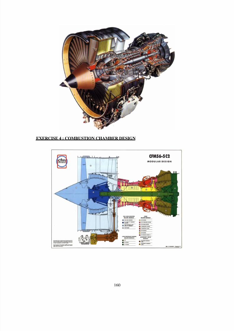
8/10/2019 Two phase flow in combustion system
http://slidepdf.com/reader/full/two-phase-flow-in-combustion-system 160/177
160
EXERCISE 4 : COMBUSTION CHAMBER DESIGN
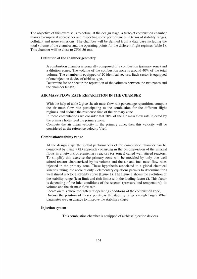
8/10/2019 Two phase flow in combustion system
http://slidepdf.com/reader/full/two-phase-flow-in-combustion-system 161/177
161
The objective of this exercise is to define, at the design stage, a turbojet combustion chamberthanks to empirical approaches and respecting some performances in terms of stability ranges,pollutant and noise emissions. The chamber will be defined from a data base including thetotal volume of the chamber and the operating points for the different flight regimes (table 1).
This chamber will be close to CFM 56 one.
Definition of the chamber geometry
A combustion chamber is generally composed of a combustion (primary zone) anda dilution zones. The volume of the combustion zone is around 40% of the totalvolume. The chamber is equipped of 20 identical sectors. Each sector is equippedof one injection device of airblast type.Determine for one sector the repartition of the volumes between the two zones andthe chamber length..
AIR MASS FLOW RATE REPARTITION IN THE CHAMBER
With the help of table 2 give the air mass flow rate percentage repartition, computethe air mass flow rate participating to the combustion for the different flightregimes and deduce the residence time of the primary zone.In these computations we consider that 50% of the air mass flow rate injected bythe primary holes feed the primary zone.Compute the air mean velocity in the primary zone, then this velocity will beconsidered as the reference velocity Vref.
Combustion/stability range
At the design stage the global performances of the combustion chamber can becomputed by using a 0D approach consisting in the decomposition of the internalflows in a network of elementary reactors (or zones) called well stirred reactors.To simplify this exercise the primary zone will be modeled by only one wellstirred reactor characterized by its volume and the air and fuel mass flow ratesinjected in the primary zone. These hypothesis associated to a global chemicalkinetics taking into account only 2 elementary equations permits to determine for awell stirred reactor a stability curve (figure 1). The figure 1 shows the evolution ofthe stability range (lean limit and rich limit) with the loading factor Ω. This factoris depending of the inlet conditions of the reactor (pressure and temperature), itsvolume and the air mass flow rate.Locate on this curve the different operating conditions of the combustion zone,
Discuss the position of theses points, is the stability range enough large? Whatparameter we can change to improve the stability range?
Injection system
This combustion chamber is equipped of airblast injection devices.

8/10/2019 Two phase flow in combustion system
http://slidepdf.com/reader/full/two-phase-flow-in-combustion-system 162/177
162
Compute the droplets Sauter Mean Diameter for the different flight regimesusing the following correlation:
55.045.025.02 ) / (040,0) / (01.2)( jk lllag jk l d V d m DMS ρ σ µ ρ σ +=
In this case aV is the air shear flow velocity inside the airblast. The
value of this velocity will be computed knowing the effective air section insidethe injection device aireff S = 300 2
mm , The fuel section jk S is a ring of
300 m µ thickness and 1cm of diameter. jk d corresponds in this correlation to
the liquid sheet thickness.
Can some droplets break up by secondary atomization effect?Remark : In this case the air velocity reference Vref must be considered
and the droplet velocity is supposed equal to the liquid sheet velocity Vl
Droplet evaporation
Compute the droplet evaporation time evτ ( D2law) for all the regimes
before ignition in the following two cases:- without taking into account convection
- with convection effect the air velocity will be the reference velocityVref and the droplet velocity will Vl.(liquid sheet velocity)And compare to the air residence time τ of the primary zone and to the
droplet relaxation time Pτ
Comments ? ?
Temperature inside the combustion zone Tpz
This temperature is computed from the adiabatic flame temperature Tstoi(enthalpy balance, table 3) and the inlet temperature T3.
Tpz = 0.9*Tstoi+0.1*T3
Compute Tpz
Pollutant emissions predictions
Mongia et de Risk correlation are often used to predict the pollutant emissions,these correlation are built on the main flow parameters of the operating point and onthe characteristic times of the two phase flows:
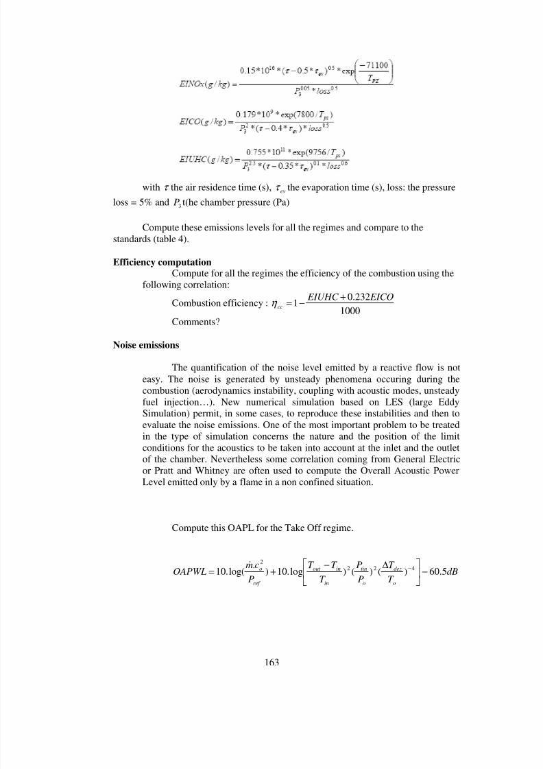
8/10/2019 Two phase flow in combustion system
http://slidepdf.com/reader/full/two-phase-flow-in-combustion-system 163/177
163
with τ the air residence time (s), evτ the evaporation time (s), loss: the pressure
loss = 5% and 3P t(he chamber pressure (Pa)
Compute these emissions levels for all the regimes and compare to thestandards (table 4).
Efficiency computationCompute for all the regimes the efficiency of the combustion using the
following correlation:
Combustion efficiency :1000
232.01
EICO EIUHC cc
+−=η
Comments?
Noise emissions
The quantification of the noise level emitted by a reactive flow is noteasy. The noise is generated by unsteady phenomena occuring during thecombustion (aerodynamics instability, coupling with acoustic modes, unsteady
fuel injection…). New numerical simulation based on LES (large EddySimulation) permit, in some cases, to reproduce these instabilities and then toevaluate the noise emissions. One of the most important problem to be treatedin the type of simulation concerns the nature and the position of the limitconditions for the acoustics to be taken into account at the inlet and the outletof the chamber. Nevertheless some correlation coming from General Electricor Pratt and Whitney are often used to compute the Overall Acoustic PowerLevel emitted only by a flame in a non confined situation.
Compute this OAPL for the Take Off regime.
dBT
T
P
P
T
T T
P
cmOAPWL
o
dez
o
tin
in
inout
ref
o 5.60)()()log.10).
log(.10 4222
−
∆−+= −&
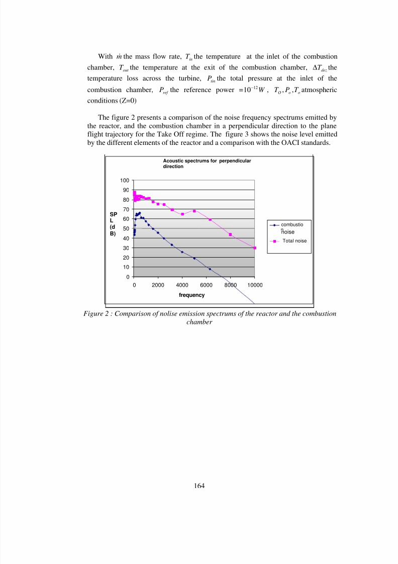
8/10/2019 Two phase flow in combustion system
http://slidepdf.com/reader/full/two-phase-flow-in-combustion-system 164/177
164
With m& the mass flow rate, inT the temperature at the inlet of the combustion
chamber, out T the temperature at the exit of the combustion chamber, dez
T ∆ the
temperature loss across the turbine, tinP the total pressure at the inlet of the
combustion chamber, ref P the reference power = W 1210− , ooO
T PT ,, atmospheric
conditions (Z=0)
The figure 2 presents a comparison of the noise frequency spectrums emitted bythe reactor, and the combustion chamber in a perpendicular direction to the planeflight trajectory for the Take Off regime. The figure 3 shows the noise level emittedby the different elements of the reactor and a comparison with the OACI standards.
Acoustic spectrums for perpendiculardirection
0
10
20
30
40
50
60
70
80
90
100
0 2000 4000 6000 8000 10000
frequency
SPL(d
B)
combustio
noise
Total noise
Figure 2 : Comparison of nolise emission spectrums of the reactor and the combustion
chamber
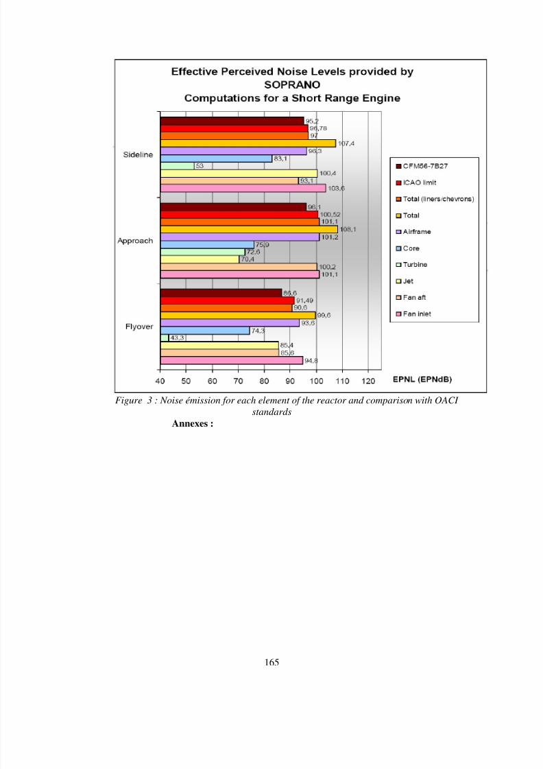
8/10/2019 Two phase flow in combustion system
http://slidepdf.com/reader/full/two-phase-flow-in-combustion-system 165/177
165
Figure 3 : Noise émission for each element of the reactor and comparison with OACIstandards
Annexes :

8/10/2019 Two phase flow in combustion system
http://slidepdf.com/reader/full/two-phase-flow-in-combustion-system 166/177
166
Figure 1 : Stability range
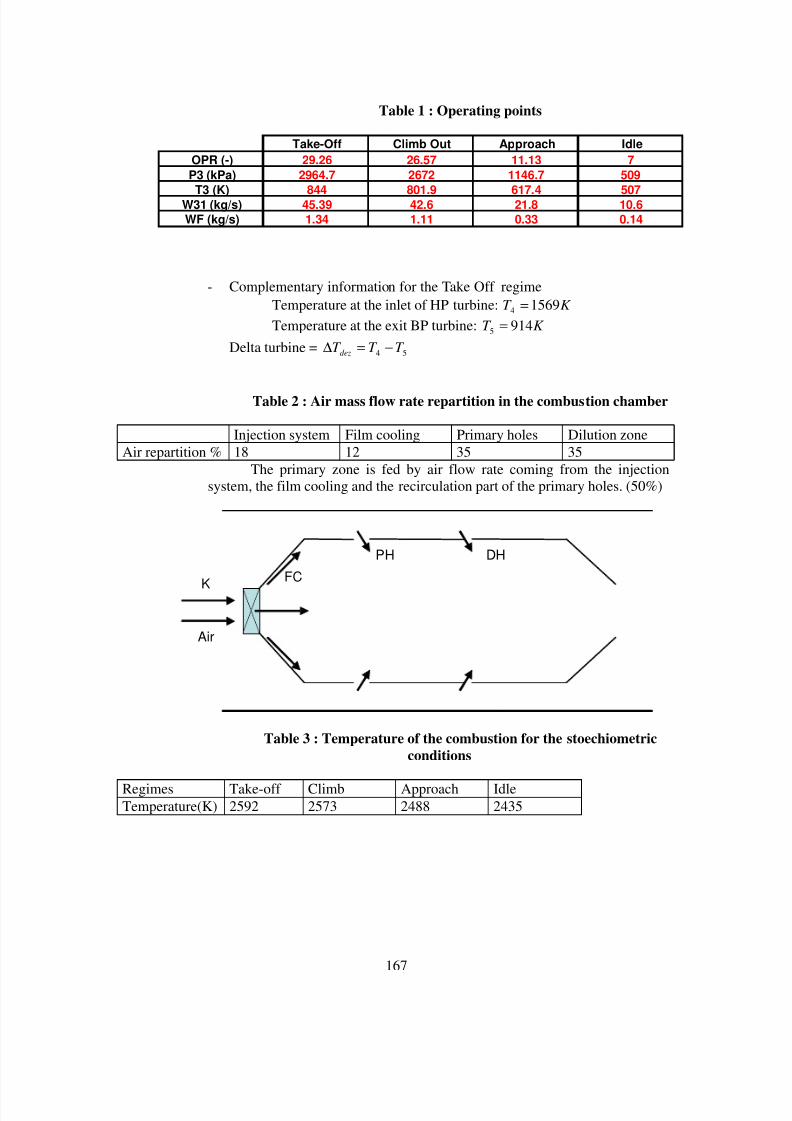
8/10/2019 Two phase flow in combustion system
http://slidepdf.com/reader/full/two-phase-flow-in-combustion-system 167/177
167
Table 1 : Operating points
- Complementary information for the Take Off regimeTemperature at the inlet of HP turbine: K T 15694 =
Temperature at the exit BP turbine: K T 9145 =
Delta turbine = 54 T T T dez −=∆
Table 2 : Air mass flow rate repartition in the combustion chamber
Injection system Film cooling Primary holes Dilution zoneAir repartition % 18 12 35 35
The primary zone is fed by air flow rate coming from the injectionsystem, the film cooling and the recirculation part of the primary holes. (50%)
FC
PH DH
K
Air
Table 3 : Temperature of the combustion for the stoechiometricconditions
Regimes Take-off Climb Approach IdleTemperature(K) 2592 2573 2488 2435
Take-Off Climb Out Approach Idle
OPR (-) 29.26 26.57 11.13 7
P3 (kPa) 2964.7 2672 1146.7 509
T3 (K) 844 801.9 617.4 507W31 (kg/s) 45.39 42.6 21.8 10.6
WF (kg/s) 1.34 1.11 0.33 0.14
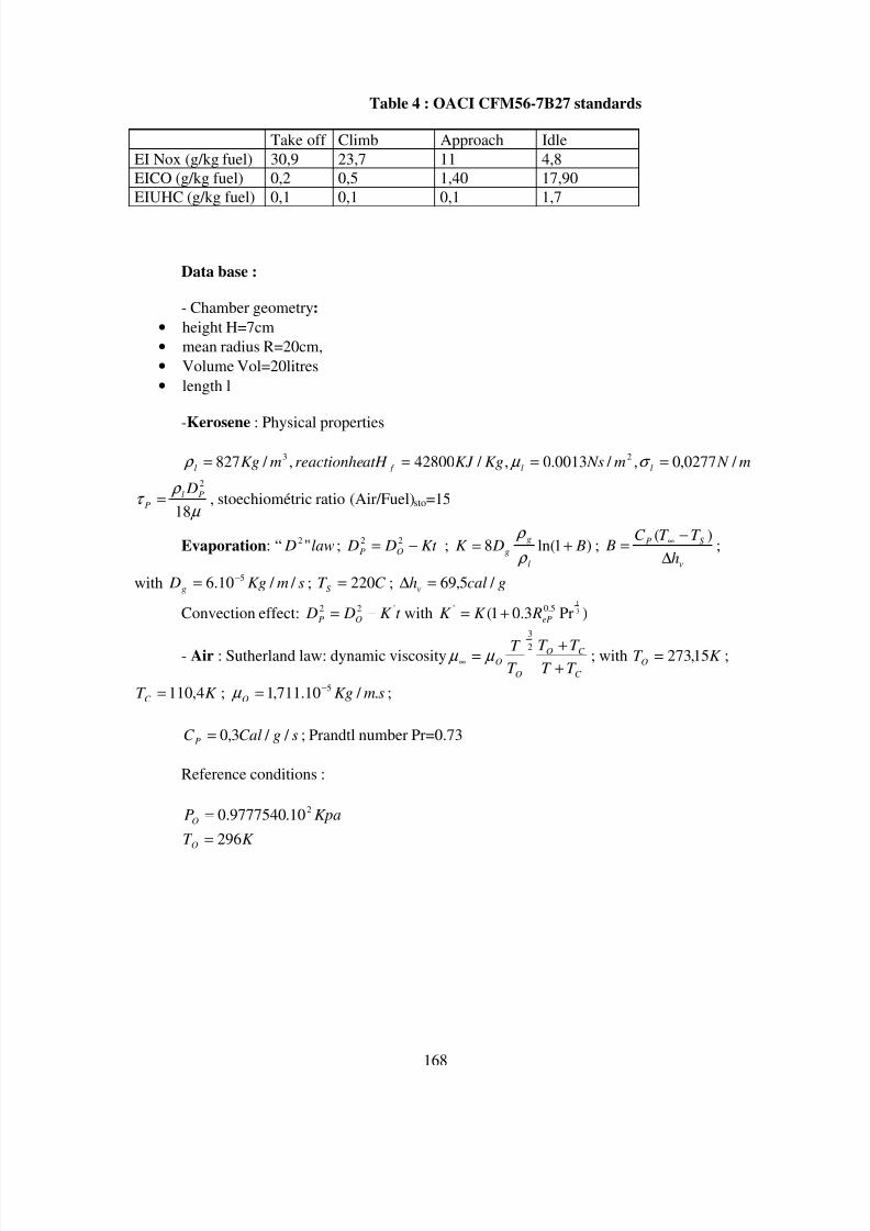
8/10/2019 Two phase flow in combustion system
http://slidepdf.com/reader/full/two-phase-flow-in-combustion-system 168/177

8/10/2019 Two phase flow in combustion system
http://slidepdf.com/reader/full/two-phase-flow-in-combustion-system 169/177
169
EXERCISE 5: DROPLET TRAJECTORIES IN AN ACOUSTIC FIELD
The coupling between acoustic field and combustion has a great influence on the repartitionof fuel droplets and on the combustion regions. To get a precise repartition of the fuel in thecase of presence of high acoustic field, the droplets trajectories must be well modeled.
In this exercise a Euler-Lagrange approach is proposed. Three levels of complexity aregenerally encountered in the two phase flow modeling depending of the volumetric flow rateratio between the two phases. In the present application, only “one-way coupling” approachwill be used (diluted two phase flows) and, thus, the fundamental dynamic equation will besolved for each droplet.
This exercise deals with the behavior of a droplet injected in a liquid propellant rocket enginewith normal working condition or submitted to high frequency combustion instabilities. Thegoal is to test the influence of combustion instabilities or more generally of an acoustic fieldon droplet lateral dispersion.
The Basset-Boussinesq and Oseen’s equation (BBO)
Question 1
From the fundamental dynamic equation, write the Basset-Boussinesq and Oseen’s equationfor the movement of a particle in any environment. Explain the different terms.
Simplification of the BBO’s equation
Generally, for combustion applications, three terms are preponderant in BBO’s equation: theinertia term, the drag force and the gravity force. Thus, a simplified BBO’s equation is used:
( ) p p
p p
f pU U U U
D
Cd
dt
U d −−=
ρ
ρ
4
3
Some experimental correlations have been proposed. For isolated droplets, the Virepinte’s one (1999) is:
( )687,012,0124
p
p
Re Re
Cd +=
Stokes equation
Introduction
When the Reynolds’ number is very low (typically when droplet relative velocity is low):
1<<−
= f
p p f
p
DU U Re
µ
ρ
Stokes (1831) has proposed a simplified drag coefficient:
p Re
Cd 24
=
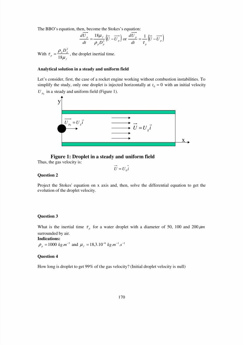
8/10/2019 Two phase flow in combustion system
http://slidepdf.com/reader/full/two-phase-flow-in-combustion-system 170/177
170
The BBO’s equation, then, become the Stokes’s equation:
( ) p
p p
f pU U
Ddt
U d −=
2
18
ρ
µ or ( ) p
p
pU U
dt
U d −=
τ
1
With f
p p
p
D
µ
ρ τ
18
2
= , the droplet inertial time.
Analytical solution in a steady and uniform field
Let’s consider, first, the case of a rocket engine working without combustion instabilities. Tosimplify the study, only one droplet is injected horizontally at 00 =t with an initial velocity
0 pU in a steady and uniform field (Figure 1).
iU U g
r
=
iU U g p
r
=0
y
x
Figure 1: Droplet in a steady and uniform field
Thus, the gas velocity is:
iU U 0=
Question 2
Project the Stokes' equation on x axis and, then, solve the differential equation to get theevolution of the droplet velocity.
Question 3
What is the inertial time pτ for a water droplet with a diameter of 50, 100 and 200 m µ
surrounded by air.Indications:
1000= p ρ 3. −mkg and 610.3,18 −= f µ 11.. −− smkg
Question 4
How long is droplet to get 99% of the gas velocity? (Initial droplet velocity is null)
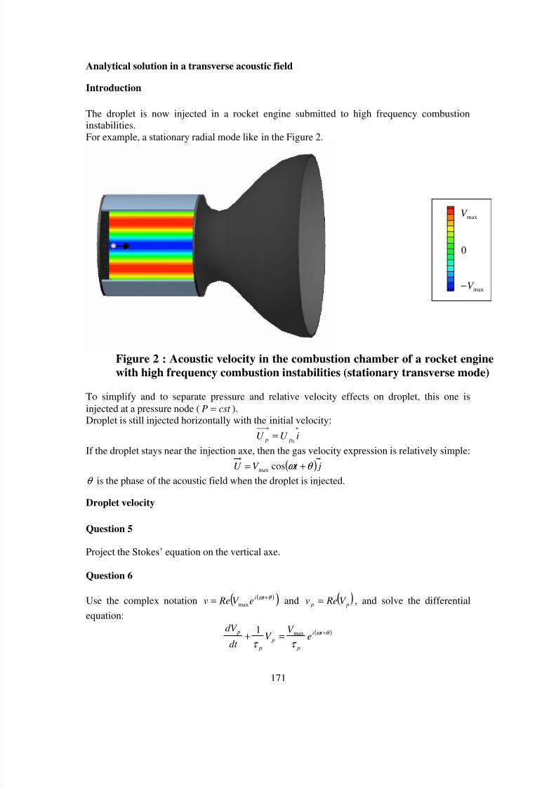
8/10/2019 Two phase flow in combustion system
http://slidepdf.com/reader/full/two-phase-flow-in-combustion-system 171/177
171
Analytical solution in a transverse acoustic field
Introduction
The droplet is now injected in a rocket engine submitted to high frequency combustioninstabilities.
For example, a stationary radial mode like in the Figure 2.
maxV
maxV −
0
Figure 2 : Acoustic velocity in the combustion chamber of a rocket enginewith high frequency combustion instabilities (stationary transverse mode)
To simplify and to separate pressure and relative velocity effects on droplet, this one is
injected at a pressure node ( cst P = ).Droplet is still injected horizontally with the initial velocity:
iU U p p 0
=
If the droplet stays near the injection axe, then the gas velocity expression is relatively simple:
( ) jt V U θ ω += cosmax
θ is the phase of the acoustic field when the droplet is injected.
Droplet velocity
Question 5
Project the Stokes’ equation on the vertical axe.
Question 6
Use the complex notation ( )( )θ ω += t ieV Rev max and p p V Rev = , and solve the differential
equation:
( )θ ω
τ τ
+=+ t i
p
p
p
pe
V V
dt
dV max1
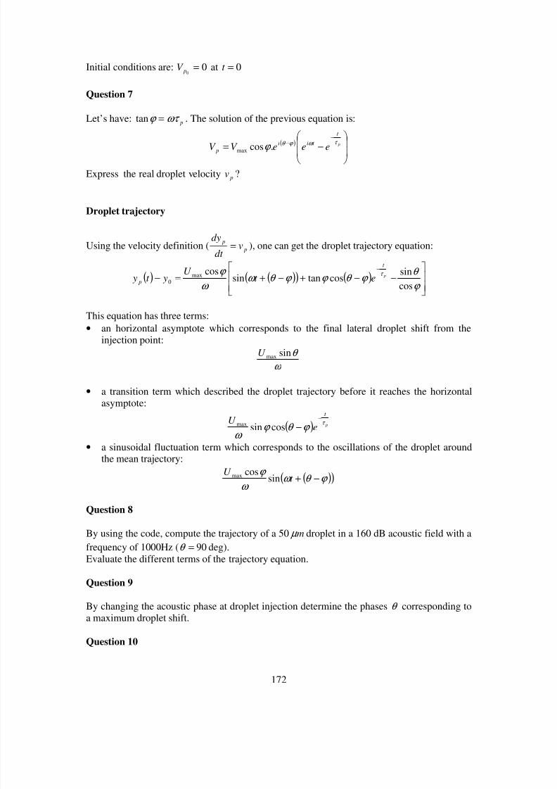
8/10/2019 Two phase flow in combustion system
http://slidepdf.com/reader/full/two-phase-flow-in-combustion-system 172/177
172
Initial conditions are: 00
= pV at 0=t
Question 7
Let’s have: pωτ ϕ =tan . The solution of the previous equation is:
( )
−=−− p
t
t ii
p eeeV V τ ω ϕ θ ϕ .cosmax
Express the real droplet velocity pv ?
Droplet trajectory
Using the velocity definition ( p
pv
dt
dy= ), one can get the droplet trajectory equation:
( ) ( )( ) ( )
−−+−+=−
−
ϕ θ ϕ θ ϕ ϕ θ ω
ω ϕ τ
cossincostansincosmax0 p
t
p et U yt y
This equation has three terms:• an horizontal asymptote which corresponds to the final lateral droplet shift from the
injection point:θ sinmaxU
• a transition term which described the droplet trajectory before it reaches the horizontalasymptote:
( ) p
t
eU τ
ϕ θ ϕ ω
−
−cossinmax
• a sinusoidal fluctuation term which corresponds to the oscillations of the droplet aroundthe mean trajectory:
( )( )ϕ θ ω ω
ϕ −+t
U sin
cosmax
Question 8
By using the code, compute the trajectory of a 50 m µ droplet in a 160 dB acoustic field with afrequency of 1000Hz ( 90=θ deg).Evaluate the different terms of the trajectory equation.
Question 9
By changing the acoustic phase at droplet injection determine the phases θ corresponding toa maximum droplet shift.
Question 10

8/10/2019 Two phase flow in combustion system
http://slidepdf.com/reader/full/two-phase-flow-in-combustion-system 173/177
173
Test the influence of droplet diameter on these three terms.
Question 11
Increase the acoustic level and, then, the acoustic frequency.
Do some comments.
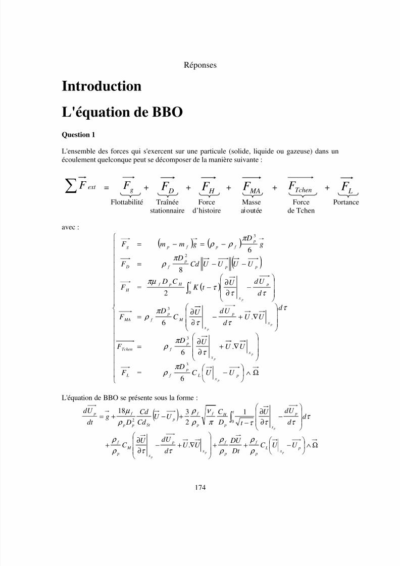
8/10/2019 Two phase flow in combustion system
http://slidepdf.com/reader/full/two-phase-flow-in-combustion-system 174/177
174
Réponses
Introduction
L'équation de BBOQuestion 1
L'ensemble des forces qui s'exercent sur une particule (solide, liquide ou gazeuse) dans unécoulement quelconque peut se décomposer de la manière suivante :
avec :
( ) ( )
( )
( )
τ
π ρ
τ
π ρ
τ τ
π ρ
τ τ τ
πµ
π ρ
π ρ ρ
d
U U C D
F
U U U D
F
U U d
U d U C
DF
d
U d U t K
C DF
U U U U Cd D
F
g D
gmmF
p x
L
p
f L
x x
p
f Tchen
x
p
x
M
p
f MA
t p
x
H p f
H
p p
p
f D
p
f p f pg
p
p
p
p
p
p
Ω∧
−=
∇+
∂
∂=
∇+−
∂
∂=
−
∂
∂−=
−−=
−=−=
∫
6
.6
.6
2
8
6
3
3
3
0
2
3
L'équation de BBO se présente sous la forme :
( )
Ω∧
−++
∇+−
∂
∂+
−
∂
∂
−+−+= ∫
p x
L
p
f
p
f
x
p
x
M
p
f
t p
x p
H f
p
f
p
St p p
f p
U U C Dt
U DU U
d
U d U C
d d
U d U
t D
C U U
Cd
Cd
Dg
dt
U d
p p
p
p
ρ
ρ
ρ
ρ
τ τ ρ
ρ
τ τ τ τ π
ν
ρ
ρ
ρ
µ
.
1
2
31802
Flottabilité Traînéestationnaire
Forced’histoire
Massea outée
Forcede Tchen
Portance
∑ ext F = gF DF H F MAF TchenF LF + + + + +
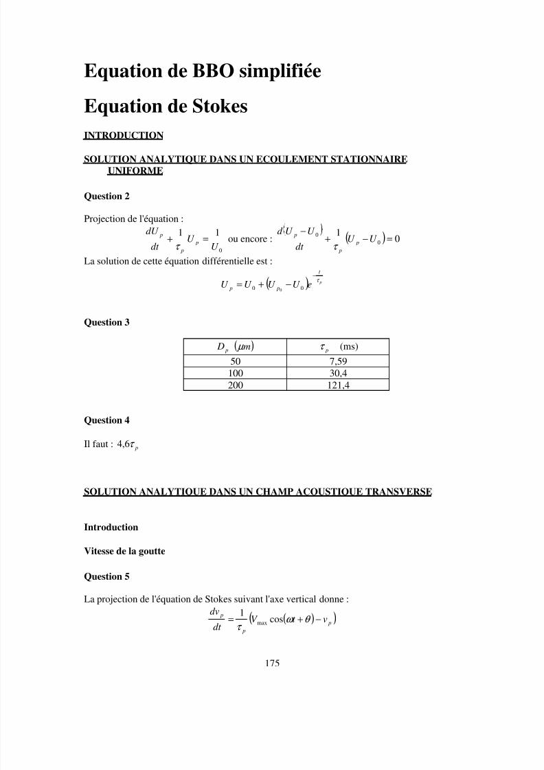
8/10/2019 Two phase flow in combustion system
http://slidepdf.com/reader/full/two-phase-flow-in-combustion-system 175/177
175
Equation de BBO simplifiée
Equation de Stokes
INTRODUCTION
SOLUTION ANALYTIQUE DANS UN ECOULEMENT STATIONNAIREUNIFORME
Question 2
Projection de l'équation :
0
11U
U dt
dU p
p
p=+
τ ou encore : ( ) 0
10
0=−+
−U U
dt
U U d p
p
p
τ
La solution de cette équation différentielle est :
( ) p
t
p p eU U U U τ
−
−+= 00 0
Question 3
p D ( )m µ p
τ (ms)
50 7,59100 30,4200 121,4
Question 4
Il faut : pτ 6,4
SOLUTION ANALYTIQUE DANS UN CHAMP ACOUSTIQUE TRANSVERSE
Introduction
Vitesse de la goutte
Question 5
La projection de l'équation de Stokes suivant l'axe vertical donne :
( )( ) p
p
pvt V
dt
dv−+= θ ω
τ cos
1max
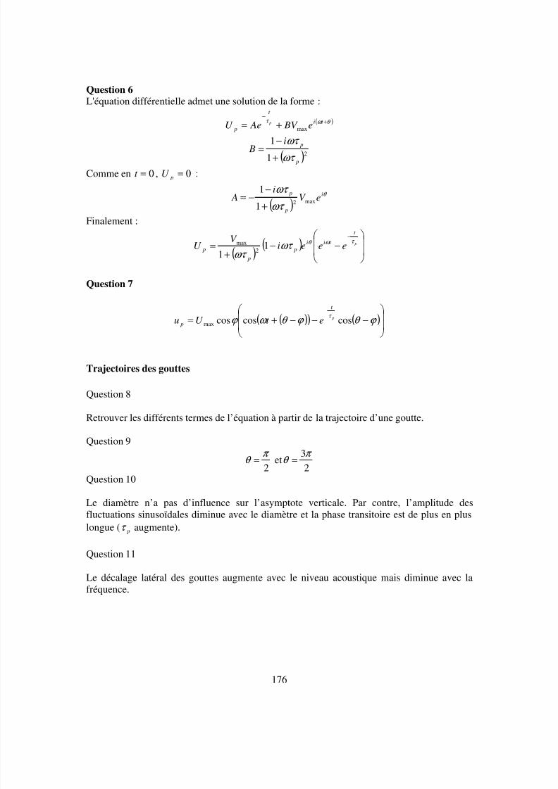
8/10/2019 Two phase flow in combustion system
http://slidepdf.com/reader/full/two-phase-flow-in-combustion-system 176/177
176
Question 6L'équation différentielle admet une solution de la forme :
( )θ ω τ +−
+= t i
t
p e BV AeU p
max
( )211
p
pi B
ωτ
ωτ
+
−=
Comme en 0=t , 0= pU :
( )θ
ωτ
ωτ i
p
peV
i A max21
1
+
−−=
Finalement :
( ) ( )
−−
+=
− p
t
t ii
p
p
p eeeiV
U τ ω θ ωτ
ωτ 1
1 2max
Question 7
( )( ) ( )
−−−+=
−
ϕ θ ϕ θ ω ϕ τ
coscoscosmax p
t
p et U u
Trajectoires des gouttes
Question 8
Retrouver les différents termes de l’équation à partir de la trajectoire d’une goutte.
Question 9
2
π θ = et
2
3π θ =
Question 10
Le diamètre n’a pas d’influence sur l’asymptote verticale. Par contre, l’amplitude desfluctuations sinusoïdales diminue avec le diamètre et la phase transitoire est de plus en pluslongue ( pτ augmente).
Question 11
Le décalage latéral des gouttes augmente avec le niveau acoustique mais diminue avec lafréquence.
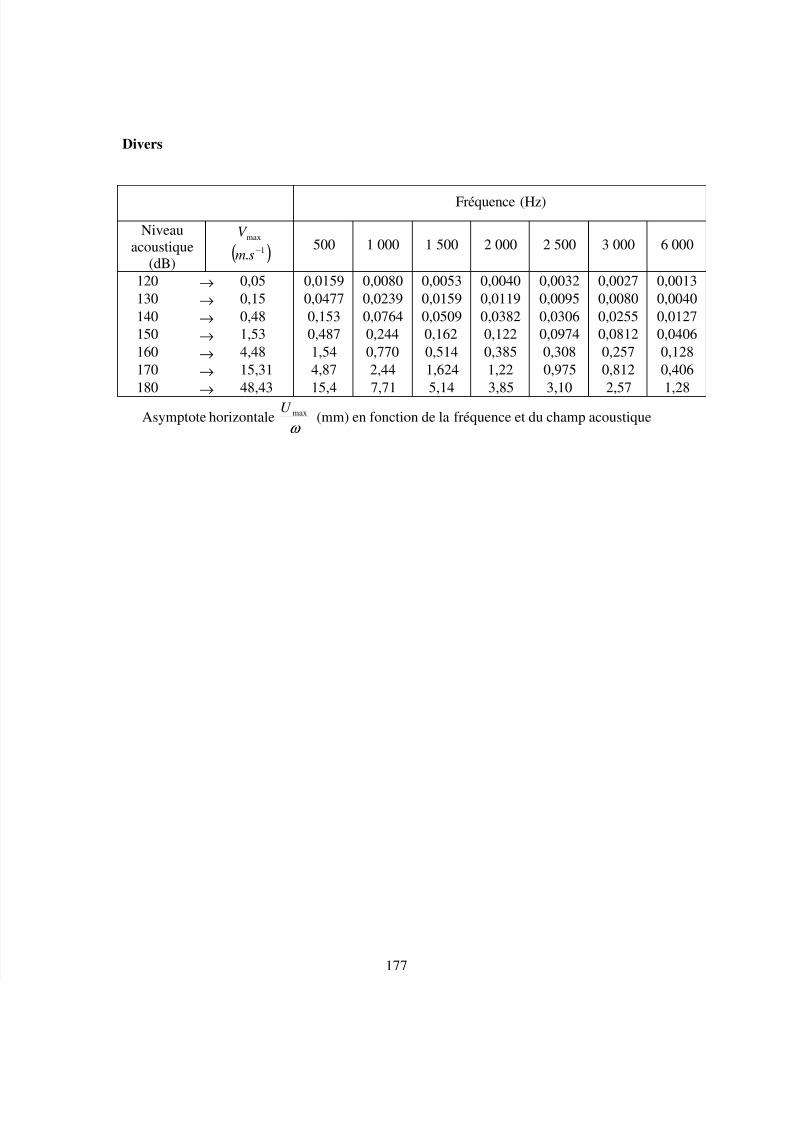
8/10/2019 Two phase flow in combustion system
http://slidepdf.com/reader/full/two-phase-flow-in-combustion-system 177/177


