Two-point Linkage Analysis

Jiankang Wang E-mail: jkwang@cgiar.org; wangjiankang@caas.cn

Web: http://www.isbreeding.net

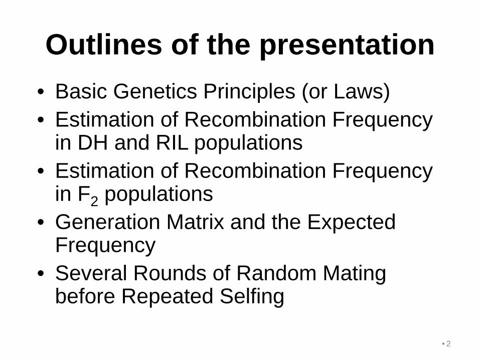
Outlines of the presentation • Basic Genetics Principles (or Laws) • Estimation of Recombination Frequency

in DH and RIL populations • Estimation of Recombination Frequency

in F2 populations • Generation Matrix and the Expected

Frequency • Several Rounds of Random Mating

before Repeated Selfing

•2

Basic Genetics Principles (or Laws)

•3

The First Mendelian Law

• The Principle of Segregation (The “First Law”).

• For genotype Aa: – From zygote to gamete:

½A + ½ a (1:1) – From gamete to zygote:

(½A + ½a)2 = ¼AA + ½Aa + ¼aa (1:2:1)

The Second Mendelian Law • For two independent loci, i.e. no

linkage • The Principle of Independent

Assortment (The “Second Law”) • For genotype AaBb:

– From zygote to gamete: ¼AB + ¼Ab + ¼aB + ¼ab (1:1:1:1)

– From gamete to zygote: (¼AB + ¼Ab + ¼aB + ¼ab)2 =_AABB +_AABb + _AAbb + _AaBB + _AaBb + _Aabb + _aaBB + _aaBb + _aabb (1:2:1:2:4:2:1:2:1)

The Third Genetics Law: Linkage and Recombination

A

a

B

b P1: AABB P2: aabb A B

a b

F1: AaBb A B

a b

×

A B a b

(1-r)/2 (1-r)/2 A b B a

r/2 r/2 Parental type Parental type Recombinant type Recombinant

type

Meiosis

Estimation of Recombination Frequency in DH and RIL

populations

•7

Populations handled in QTL IciMapping Parent P1 Parent P2 Legends

HybridizationF1

Selfing1. P1BC1F1 7. F2 2. P2BC1F1

Repeated selfing9. P1BC2F1 13. P1BC1F2 8. F3 14. P2BC1F2 10. P2BC2F1

Doubled haploids15. P1BC2F2 16. P2BC2F2

11. P1BC2RIL 5. P1BC1RIL 4. F1RIL 6. P2BC1RIL 12. P2BC2RIL BC3F1, BC4F1 etc.

P1BC2F1 P1BC1F1 F1 P2BC1F1 P2BC2F1 Marker-assistedselection

19. P1BC2DH 17. P1BC1DH 3. F1DH 18. P2BC1DH 20. P2BC2DH CSS lines orIntrogression lines

P1 × CP P2 × CP P3 × CP … Pn × CP CP=common parent

RIL family 1 RIL family 2 RIL family 3 RIL family i RIL family n

One NAM population

•9

Marker C263 R830 R3166 XNpb387 R569 R1553 C128 C1402 XNpb81 C246 R2953 C1447 Grain width (mm)

Position (cM) 0.0 3.5 8.5 19.5 32.0 66.6 74.1 78.6 81.8 91.9 92.7 96.8

RIL1 0 0 0 0 0 0 0 0 0 0 0 0 2.33

RIL2 2 2 2 2 2 0 0 0 0 2 2 2 1.99

RIL3 0 2 2 2 2 2 2 2 2 2 2 2 2.24

RIL4 0 0 0 0 0 0 2 2 2 2 2 2 1.94

RIL5 0 0 0 0 0 2 2 0 0 0 0 0 2.76

RIL6 0 0 0 2 2 2 2 2 2 2 2 2 2.32

RIL7 0 0 0 0 0 0 0 0 0 0 0 0 2.32

RIL8 2 2 0 2 2 0 0 0 0 2 2 2 2.08

RIL9 0 0 0 0 2 2 0 0 0 0 0 0 2.24

RIL10 0 0 0 0 2 2 0 0 0 0 0 0 2.45

Example: 10 RILs in a rice population (Linkage map of Chr. 5)

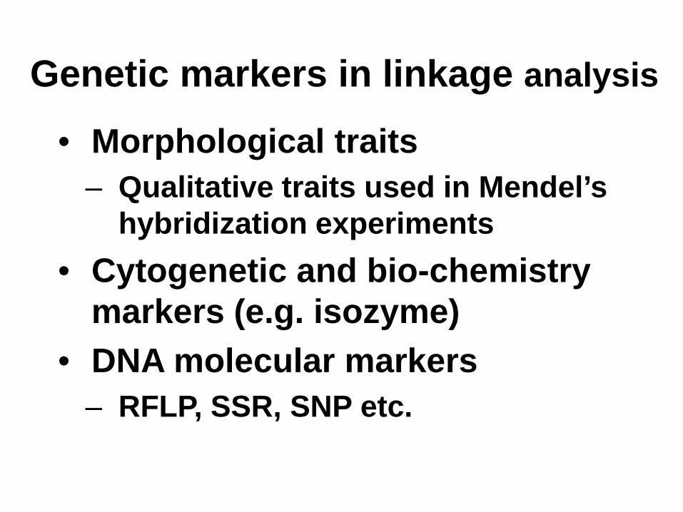
Genetic markers in linkage analysis

• Morphological traits – Qualitative traits used in Mendel’s

hybridization experiments • Cytogenetic and bio-chemistry

markers (e.g. isozyme) • DNA molecular markers

– RFLP, SSR, SNP etc.

Expected genotypic frequency in backcross and DH populations

P1: AABB; P2: aabb

•11

P1BC1 P2BC1 DH Samples Theoretical frequency

AB/AB AB/ab AB/AB n1 f1=(1-r)/2

Ab/AB Ab/ab Ab/Ab n2 f2=r/2

aB/AB aB/ab aB/aB n3 f3=r/2

ab/AB ab/ab ab/ab n4 f4=(1-r)/2

AB, Ab, aB, and ab are the 4 haplotype of F1 hybrid

MLE of recombination frequency • Likelihood function

• Logarithm of likelihood

• MLE of r • Fisher information

• Variance of estimated r

•12

3241

4321

)()1()1(21

21

21)1(

21

!!!!!

4321

nnnnnnnn

rrCrrrrnnnn

nL ++−=

−

−=

rnnrnnCL ln)()1ln()(lnln 3241 ++−++=

nnn

nnnnnnr 32

4321

32ˆ +=

++++

=

)1()1()ln( 2

32241

2

2

rrn

rnn

rnnE

rdLdEI

−=

+−

−+

−−=−=

nrr

IVr

)ˆ1(ˆ1ˆ

−==

Significance test of linkage • Null hypothesis H0: r = 0.5 (no genetic

linkage, or locus A-a and B-b are independent)

• Alternative hypothesis HA: r ≠ 0.5

• Likelihood ratio test (LRT) or LOD score

)1(~])ˆ(

)5.0(ln[2 2 ==

−= dfrL

rLLRT χ

)5.0()ˆ(log

==

rLrLLOD

An example P1BC1 population • Genotypes of two inbred parents P1 and

P2 are AABB and aabb • Observed samples of the four

genotypes in P1BC1 – AABB: 162; AABb: 40; AaBB: 41; AaBb: 158

•14

%20.2040181

15841401624140ˆ ==+++

+=r

4ˆ 1002.4)ˆ1(ˆ −×≈

−=

nrrVr

Test of linkage • Null hypothesis H0: r = 0.5 • Alternative hypothesis HA: r ≠ 0.5

• Likelihood ratio test (LRT) (P<0.0001) and

LOD score

•15

09.33])5.0(

)ˆ(log[ ==

=rL

rLLOD

37.152])ˆ(

)5.0(ln[2 ==

−=rL

rLLRT

Genotypic frequencies in RIL populations, compared with DH

•16

DH population

Theoretical frequency

RIL population

Theoretical frequency

AABB f1=(1-r)/2 AABB f1=(1-R)/2

AAbb f2=r/2 AAbb f2=R/2

aaBB f3=r/2 aaBB f3=R/2

aabb f4=(1-r)/2 aabb f4=(1-R)/2

R=2r/(1+2r)

•17

10 RILs in a rice population P1: 0 or A; P2: 2 or B; F1: 1 or H

RIL Marker 1 Marker 2 Parent type or recombinant

C263 XNpb387 RIL1 0 or A 0 or A P1 type RIL2 2 or B 2 or B P2 type RIL3 0 or A 2 or B Recombinant RIL4 0 or A 0 or A P1 type RIL5 0 or A 0 or A P1 type RIL6 0 or A 2 or B Recombinant RIL7 0 or A 0 or A P1 type RIL8 2 or B 2 or B P2 type RIL9 0 or A 0 or A P1 type RIL10 0 or A 0 or A P1 type

n1=6 n2=2 n3=0 n4=2

R=2/10=0.2

r=0.125

LRT=3.8549, (P=0.0496)

LOD=0.8371

Estimation of Recombination Frequency in F2 populations

•18

Expected genotypic frequencies in F2 populations

Co-dominant markers Dominant markers Marker type Frequency Marker type Frequency AABB (1-r)2/4 A_B_ [2+(1-r)2]/4 AABb r(1-r)/2 AAbb r2/4 A_bb [1-(1-r)2]/4 AaBB r(1-r)/2 AaBb (1-2r+2r2)/2 Aabb r(1-r)/2 aaBB r2/4 aaB_ [1-(1-r)2]/4 aaBb r(1-r)/2 aabb (1-r)2/4 aabb (1-r)2/4

Co-dominant markers in other populations

Marker type

Population

F2 P1B1F1 P2B1F1 F1DH P1BC1DH P2BC1DH F1-RIL

AABB (1-r)2/4 (1-r)/2 (1-r) /2 ½+(1-r) 2/4 (1-r) 2/4 (1-R)/2

AABb r(1-r)/2 r/2

AAbb r2/4 r/2 r/2-r 2/4 r/2-r 2/4 R/2

AaBB r(1-r)/2 r/2

AaBb (1-2r+2r2)/2 (1-r)/2 (1-r)/2

Aabb r(1-r)/2 r/2

aaBB r2/4 r/2 r/2-r 2/4 r/2-r 2/4 R/2

aaBb r(1-r)/2 r/2

aabb (1-r)2/4 (1-r)/2 (1-r) /2 (1-r) 2/4 ½+(1-r) 2/4 (1-R)/2

R=2r/(1+2r)

MLE of r in F2: dominant markers • Logarithm of the likelihood ratio

• MLE of r

• Variance of the estimated r

2)1( rk −=

)21ln()2ln()()23ln(ln 29

273

21 rrnrrnnrrnCL +−+−+++−+=

knknnknC ln)1ln()()2ln( 9731 +−++++=

nnnnnnnnn

rk2

)32()32()1( 9

291912 ×+−−±−−−

=−=

)243(2)23)(2(

)21(2)2)(1(

2

22

ˆ rrnrrrr

knkkVr +−

+−−=

+−−

=

MLE of r in F2: co-dominant markers (Newton-Raphson algorithm) • Log-likelihood function

• The first-order derivative of LogL • f'(r) • The second-order derivative of LogL • f''(r) • The iteration algorithm:

ri+1 = ri - f'(ri)/f''(ri)

)221ln(ln)22(

)1ln()22(lnln2

5738642

864291

rrnrnnnnnnrnnnnnnCL+−+++++++

−++++++=

25738642864291

221)24(22

122ln

rrrn

rnnnnnn

rnnnnnn

drLd

+−−

++++++

+−

+++++==

22

25

2738642

2864291

2

2

)221()44(22

)1(22ln)

rrrrn

rnnnnnn

rnnnnnn

rdLd

+−−

++++++

−−

+++++−==

MLE of r in F2: co-dominant markers (EM algorithm)

• EM for expectation and maximization

• E-step: for an initial r0, calculate the probability of crossover in each marker type

• M-step: Update r, and repeat from the E-step

∑=k

kkn GRPnr )|(' 1

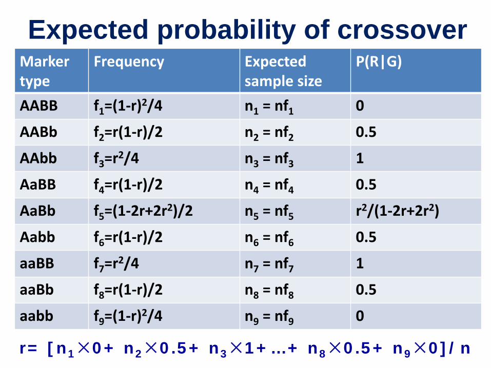
Expected probability of crossover Marker type

Frequency Expected sample size

P(R|G)

AABB f1=(1-r)2/4 n1 = nf1 0

AABb f2=r(1-r)/2 n2 = nf2 0.5

AAbb f3=r2/4 n3 = nf3 1

AaBB f4=r(1-r)/2 n4 = nf4 0.5

AaBb f5=(1-2r+2r2)/2 n5 = nf5 r2/(1-2r+2r2)

Aabb f6=r(1-r)/2 n6 = nf6 0.5

aaBB f7=r2/4 n7 = nf7 1

aaBb f8=r(1-r)/2 n8 = nf8 0.5

aabb f9=(1-r)2/4 n9 = nf9 0

r= [n1×0+ n2×0.5+ n3×1+…+ n8×0.5+ n9×0]/n

Estimated r after 3 EM iterations (r0=0.5)

Geno. Size r0 Exp. Freq. P(R|G) r1

Exp. Freq. P(R|G) r2

Exp. Freq. P(R|G) r3

AABB 30 0.5 0.063 0 0.313 0.118 0 0.198 0.161 0 0.159 AABb 7 0.5 0.125 0.5 0.313 0.107 0.5 0.198 0.080 0.5 0.159 AAbb 1 0.5 0.063 1 0.313 0.024 1 0.198 0.010 1 0.159 AaBB 9 0.5 0.125 0.5 0.313 0.107 0.5 0.198 0.080 0.5 0.159 AaBb 50 0.5 0.250 0.5 0.313 0.285 0.1712 0.198 0.341 0.0577 0.159 Aabb 12 0.5 0.125 0.5 0.313 0.107 0.5 0.198 0.080 0.5 0.159 aaBB 0 0.5 0.063 1 0.313 0.024 1 0.198 0.010 1 0.159 aaBb 10 0.5 0.125 0.5 0.313 0.107 0.5 0.198 0.080 0.5 0.159 aabb 25 0.5 0.063 0 0.313 0.118 0 0.198 0.161 0 0.159

144 1 1 1

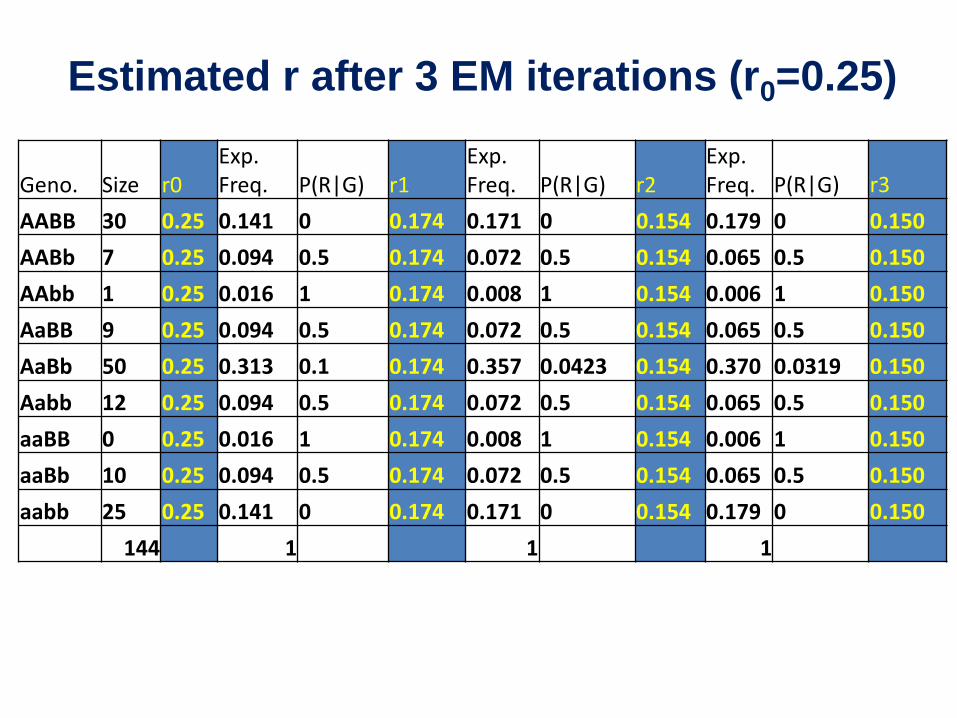
Estimated r after 3 EM iterations (r0=0.25)

Geno. Size r0 Exp. Freq. P(R|G) r1

Exp. Freq. P(R|G) r2

Exp. Freq. P(R|G) r3

AABB 30 0.25 0.141 0 0.174 0.171 0 0.154 0.179 0 0.150 AABb 7 0.25 0.094 0.5 0.174 0.072 0.5 0.154 0.065 0.5 0.150 AAbb 1 0.25 0.016 1 0.174 0.008 1 0.154 0.006 1 0.150 AaBB 9 0.25 0.094 0.5 0.174 0.072 0.5 0.154 0.065 0.5 0.150 AaBb 50 0.25 0.313 0.1 0.174 0.357 0.0423 0.154 0.370 0.0319 0.150 Aabb 12 0.25 0.094 0.5 0.174 0.072 0.5 0.154 0.065 0.5 0.150 aaBB 0 0.25 0.016 1 0.174 0.008 1 0.154 0.006 1 0.150 aaBb 10 0.25 0.094 0.5 0.174 0.072 0.5 0.154 0.065 0.5 0.150 aabb 25 0.25 0.141 0 0.174 0.171 0 0.154 0.179 0 0.150

144 1 1 1

Estimated r after 3 EM iterations (r0=0.0)

Geno. Size r0 Exp. Freq. P(R|G) r1

Exp. Freq. P(R|G) r2

Exp. Freq. P(R|G) r3

AABB 30 0 0.250 0 0.139 0.185 0 0.148 0.182 0 0.149 AABb 7 0 0.000 0.5 0.139 0.060 0.5 0.148 0.063 0.5 0.149 AAbb 1 0 0.000 1 0.139 0.005 1 0.148 0.005 1 0.149 AaBB 9 0 0.000 0.5 0.139 0.060 0.5 0.148 0.063 0.5 0.149 AaBb 50 0 0.500 0 0.139 0.380 0.0253 0.148 0.374 0.0292 0.149 Aabb 12 0 0.000 0.5 0.139 0.060 0.5 0.148 0.063 0.5 0.149 aaBB 0 0 0.000 1 0.139 0.005 1 0.148 0.005 1 0.149 aaBb 10 0 0.000 0.5 0.139 0.060 0.5 0.148 0.063 0.5 0.149 aabb 25 0 0.250 0 0.139 0.185 0 0.148 0.182 0 0.149

144 1 1 1

MLE of r in F2: between one co-dominant marker and one dominant marker

• Likelihood function

• Log-likelihood function

• The first-order derivative of LogL

• The second-order derivative of LogL

• The iteration algorithm: ri+1 = ri - f'(ri)/f''(ri)

654321 2222 )1()]2([)]1([)1()()1()( nnnnnn rrrrrrrrrCrL −−−+−−=

654321 2222 )1()]2([)]1([)1()()1()( nnnnnn rrrrrrrrrCrL −−−+−−=

)1ln()2ln()1ln()2( 235641 rrnrnrnnn +−+−+−+++

rnnn

rn

rnnn

drrLdrL

−++

−+

+++

==1

21

2)(ln)('ln 64115422

35

1)21(

2 rrrn

rn

+−−

−−

−

2641

21

2542

2

2

)1(2

)1(2)(ln)(''ln

rnnn

rn

rnnn

drrLdrL

−++

++

−++

−== 22

23

25

)1()221(

)2( rrrrn

rn

+−−+

+−

+

Principe of the Newton-Raphson algorithm

• To find the maxima of LnL is equal to find the solution in equation Ln’L=0

d(LnL)/dr or Ln'L

r(0) r(1)

lnL'(r(0))

r(2)

lnL'(r(1))O

r^

An example in wheat

•30

Resistant F2 Susceptible F2 Marker type A H B A H B Size 572 1161 14 3 22 569

Iteration 1 2 3 4 5 Recom. Freq. r 0.0010 0.0019 0.0037 0.0066 0.0108 LnL -282.75 -257.02 -234.28 -216.51 -205.69 d(LnL)/dr 39670 19268 9081.59 4018.63 1548.44 d2(LnL)/dr2 -4.12E7 -1.11E7 -3.10E6 -9.5E5 -3.58E5 Iteration 5 6 7 8 9 Recom. Freq. r 0.0108 0.0151 0.0175 0.0179 0.0179 LnL -205.69 -201.67 -201.12 -201.11 -201.11 d(LnL)/dr 1548.44 430.81 50.88 -0.26 0.0071 d2(LnL)/dr2 -3.58E5 -1.81E5 -1.35E5 -1.29E5 -1.29E5

Distortion has little effect on linkage analysis!

DH pop Theo. Freq. Distortion Freq. in distortion

AABB f1=(1-r)/2 (1-r)/2 (1-r)/(1+s)

AAbb f2=r/2 r/2 r/(1+s)

aaBB f3=r/2 s×r/2 r×s/(1+s)

aabb f4=(1-r)/2 s×(1-r)/2 (1-r)×s/(1+s)

Sum 1 (1+s)/2 1

rssrssrsrr =++=+×++= )1/()1()1/()1/(ˆ

More populations (e.g. BC1F2, F3 etc): Generation matrix

Parent Genotype and frequency in self-pollinated progeny

AABB AABb AAbb AaBB AB/ab Ab/aB Aabb aaBB aaBb aabb

AABB 1

AABb 0.25 0.5 0.25

AAbb 1

AaBB 0.25 0.5 0.25

AB/ab (1-r)2/4 r(1-r)/2 r2/4 r(1-r)/2 (1-r)2/2 r2/2 r(1-r)/2 r2/4 r(1-r)/2 (1-r)2/4

Ab/aB r2/4 r(1-r)/2 (1-r)2/4 r(1-r)/2 r2/2 (1-r)2/2 r(1-r)/2 (1-r)2/4 r(1-r)/2 r2/4

Aabb 0.25 0.5 0.25

aaBB 1

aaBb 0.25 0.5 0.25

aabb 1

Generation Matrix and the Expected Frequency

•33

Expected genotype frequencies calculated from the transmission

matrix (T)

•34

[ ])()()()()(/

)(/

)()()()()( taabb

taaBb

taaBB

tAabb

taBAb

tabAB

tAaBB

tAAbb

tAABb

tAABB

t ffffffffff=f

[ ])1()1()1()1()1(/

)1(/

)1()1()1()1()1( +++++++++++ = taabb

taaBb

taaBB

tAabb

taBAb

tabAB

tAaBB

tAAbb

tAABb

tAABB

t fffffffffff

Tff )()1( tt =+

The generation matrix (T) for the backcrossing to P1

•35

−−−−

=

00000100000000000000000010000000000000000)1(0)1(00000)1(0)1(000000000000000010000000000000000001

21

21

21

21

21

21

21

21

21

21

21

21

21

21

21

21

P1B rrrrrrrr

T

[ ])()()()()(/

)(/

)()()()()( taabb

taaBb

taaBB

tAabb

taBAb

tabAB

tAaBB

tAAbb

tAABb

tAABB

t ffffffffff=f

The generation matrix (T) for the backcrossing to P2

•36

−−−−

=

100000000000000000

010000000000000000

)1(0)1(00000)1(00)1(0000

000000000001000000000000000000010000

21

21

21

21

21

21

21

21

21

21

21

21

21

21

21

21

P2B rrrrrrrr

T

[ ])()()()()(/

)(/

)()()()()( taaBB

taaBB

taaBB

tAabb

taBAb

tabAB

tAaBB

tAAbb

tAABb

tAABB

t ffffffffff=f

The generation matrix (T) for the selfing pollination

•37

−−−−−−−−−−−−−−

=

10000000000000000

00100000000000000

)1()1()1()1()1()1()1()1()1()1()1()1()1()1(

0000000000000010000000000000000001

41

21

41

41

21

41

221

212

41

212

212

21

212

41

212

41

241

212

41

212

212

21

212

41

212

41

41

21

41

41

21

41

S rrrrrrrrrrrrrrrrrrrrrrrrrrrr

T

[ ])()()()()(/

)(/

)()()()()( taaBB

taaBB

taaBB

tAabb

taBAb

tabAB

tAaBB

tAAbb

tAABb

tAABB

t ffffffffff=f

The generation matrix (T) for the doubled haploids

•38

−−−−

=

100000000000000000

0010000000000000000)1(0000)1(0

)1(000000)1(000000000000000100000000000000000001

21

21

21

21

21

21

21

21

21

21

21

21

21

21

21

21

D rrrrrrrr

T

[ ])()()()()(/

)(/

)()()()()( taaBB

taaBB

taaBB

tAabb

taBAb

tabAB

tAaBB

tAAbb

tAABb

tAABB

t ffffffffff=f

The generation matrix (T) for the repeated selfing pollination

•39

−−−−

=

100000000000000000

0010000000000000000)1(0000)1(0

)1(000000)1(000000000000000100000000000000000001

21

21

21

21

21

21

21

21

21

21

21

21

21

21

21

21

R RRRRRRRR

T

[ ])()()()()(/

)(/

)()()()()( taaBB

taaBB

taaBB

tAabb

taBAb

tabAB

tAaBB

tAAbb

tAABb

tAABB

t ffffffffff=f

Theoretical frequencies of

the 20 biparental

populations

•40

[ ]0000010000)0( =fNo. Population Theoretical frequencies 1 P1BC1F1 f(0)×TP1B 2 P2BC1F1 f(0)×TP2B 3 F1DH f(0)×TD 4 F1RIL f(0)×TR 5 P1BC1RIL f(0)×TP1B×TR 6 P2BC1RIL f(0)×TP1B×TR 7 F2 f(0)×TS 8 F3 f(0)×TS×TS 9 P1BC2F1 f(0)×TP1B×TP1B 10 P2BC2F1 f(0)×TP2B×TP2B 11 P1BC2RIL, f(0)×TP1B×TP1B×TR 12 P2BC2RIL, f(0)×TP2B×TP2B×TR 13 P1BC1F2 f(0)×TP1B×TS 14 P2BC1F2 f(0)×TP2B×TS 15 P1BC2F2 f(0)×TP1B×TP1B×TS 16 P2BC2F2 f(0)×TP2B×TP2B×TS 17 P1BC1DH f(0)×TP1B×TD 18 P2BC1DH f(0)×TP2B×TD 19 P1BC2DH f(0)×TP1B×TP1B×TD 20 P2BC2DH f(0)×TP2B×TP2B×TD

In formulas, …

•41

Several Rounds of Random Mating before Repeated Selfing

•42

How about several rounds of random mating before the repeated selfing?

• The IBM population of maize: – B73 and Mo17 are the two parental lines – RILs, but there are 4 rounds of random mating

before the repeated selfing, therefore was named IBM

• Random mating can enlarge the recombination frequency, so that close linkage may be separated.

•43

Accumulated recombination frequency

•44

Rounds of random mating (t) Mapping distance (cM) 1 (=F2) 1.00 2.00 5.00 2 1.50 2.99 7.44 3 2.00 3.98 9.88 4 2.49 4.97 12.31 5 2.99 5.96 14.75 6 3.49 6.95 17.19 7 3.99 7.94 19.63 8 4.48 8.93 22.06 9 4.98 9.92 24.50 10 5.48 10.91 26.94 F1-RIL 1.98 3.92 9.55

141 )1)(21( −−−= t

t rrD

Frequencies of AABB, AAbb, aaBB and aabb in RILs?!

• From genotype frequencies (10 genotypes), work out haplotype frequencies (4 haplotypes)

• Work out the haplotype frequencies (4 haplotypes) after several rounds of random mating from Dt=D1(1-r)t-1, i.e.

• Work out genotype frequencies • Use generation matrix TR to find out the genotype

frequencies in RILs • The genetic analysis can be very complicated

even with biparental populations!

•45

tt Dfff += BA)(

AB tt Dfff −= bA)(

Ab tt Dfff −= Ba)(

aB tt Dfff += ba)(

ab

A dominant resistance gene is linked with a co-dominant molecular marker

F2 population Resistant Susceptible Marker type A H B A H B Sample size 572 1161 14 3 22 569 Marker types A and B are parental types; H is the type of F1 hybrid

Resistant and susceptible can be fitted by the 3:1 ratio (one dominance gene locus): χ2=0.17 (P=0.68). Marker types A, H, and B can be fitted by the 1:2:1 ratio (one co-dominance gene locus) : χ2=0.32 (df=2, P=0.85)

But Resistance and Marker are not independent, i.e. can not be fitted by the 3:6:3:1:2:1 ratio.

The genetic distance between the gene and marker is estimated at 1.8 cM

•47

Resistant F2 Susceptible F2 Marker type

A H B A H B

Size 572 1161 14 3 22 569

The genetic distance is at 1.8 cM

•48

Resistant F2 Susceptible F2 Marker type A H B A H B Size 572 1161 14 3 22 569

1/3 of Susceptible Marker type A H B A H B Size 572 1161 14 1 7 190

Dominant marker Marker type AH B AH B Size 1733 14 25 569

Recessive marker Marker type A HB A HB Size 572 1175 3 591