Two Sample Inference for Populations of Graphical Models ... · PDF fileover network edges...

arXiv: 0000.0000

TWO SAMPLE INFERENCE FOR POPULATIONS OF GRAPHICAL MODELSWITH APPLICATIONS TO FUNCTIONAL CONNECTIVITY

BY MANJARI NARAYAN∗ , GENEVERA I. ALLEN∗,†,‡ AND STEFFIE N. TOMSON§

Dept. of Electrical Engineering∗ & Dept. of Statistics, Rice University†,Dept. of Pediatrics-Neurology, Baylor College of Medicine & Jan and Dan Duncan Neurological

Research Institute, Texas Children’s Hospital‡, Dept. of Psychiatry, UCLA§

Abstract Gaussian Graphical Models (GGM) are popularly used inneuroimaging studies based on fMRI, EEG or MEG to estimate func-tional connectivity, or relationships between remote brain regions. Inmulti-subject studies, scientists seek to identify the functional brainconnections that are different between two groups of subjects, i.e. con-nections present in a diseased group but absent in controls or viceversa. This amounts to conducting two-sample large scale inferenceover network edges post graphical model selection, a novel problemwe call Population Post Selection Inference. Current approaches to thisproblem include estimating a network for each subject, and then as-suming the subject networks are fixed, conducting two-sample infer-ence for each edge. These approaches, however, fail to account for thevariability associated with estimating each subject’s graph, thus re-sulting in high numbers of false positives and low statistical power.By using resampling and random penalization to estimate the post se-lection variability together with proper random effects test statistics,we develop a new procedure we call R3 that solves these problems.Through simulation studies we show that R3 offers major improve-ments over current approaches in terms of error control and statisti-cal power. We apply our method to identify functional connectionspresent or absent in autistic subjects using the ABIDE multi-subjectfMRI study.

1. Introduction. Functional connectivity seeks to find statistical dependencies betweenneural activity in different parts of the brain (Smith, 2012; Smith et al., 2013). It has beenstudied at a systems or whole brain level using noninvasive imaging techniques such asfunctional MRI (fMRI), EEG and MEG, or using more invasive techniques at the micro levelsuch as electrophysiology or ECoG. Whole brain functional connectivity has become espe-cially popular to study in resting state fMRI where subjects lie in the scanner passively atrest (Smith, 2012). For this data, connectivity is typically modeled as a network with func-tionally or anatomically derived brain regions as nodes and connections as undirected edges(Bullmore and Sporns, 2009). In this paper, we are particularly interested in studying multi-subject functional connectivity for resting-state fMRI data; the statistical challenges we out-line and methods we develop, however, are applicable to functional connectivity in manyneuroimaging modalities.

Many have sought to use functional connectivity and more broadly connectomics to bet-ter understand neurological conditions and diseases. Specifically, we seek to address thequestion - How are functional connections different in a group of diseased subjects thanin healthy controls? - by conducting inference across a population of brain networks. This

MSC 2010 subject classifications: functional connectivity, neuroimaging, graphical models, random effects, postselection inference, population post selection inference

1

arX

iv:1

502.

0385

3v1

[st

at.M

E]

12

Feb

2015

http://arxiv.org/abs/0000.0000

2 NARAYAN ET AL.

question has been well studied in the neuroimaging literature; see (Milham, 2012; Crad-dock et al., 2013) for detailed reviews. Indeed, neuroscientists have used these techniquesto find connectivity biomarkers for diseases such as Alzheimer’s and clinical depression(Tam et al., 2014; Tao et al., 2013). However, we will show that these widely used methodssuffer from major statistical flaws that can result in high error rates. Understanding and solv-ing these flaws presents us with a new type of statistical problem, something that we willterm Population Post Selection Inference (popPSI), that has been previously unaddressed in thestatistics literature. Thus in this paper, we have three major objectives: (1) To introduce thiscompletely new problem that arises in population functional connectivity to the statisticalcommunity; (2) To discuss the open statistical challenges that arise with this problem anddiagnosis problems associated with the currently used methods in neuroimaging; and (3)To introduce a new statistical method that partially solves these problems, leading to muchimproved performance in terms of statistical power and error control.

1.1. Current Standard in Neuroimaging. Before proceeding to define our problem, we pauseto understand current approaches in the neuroimaging literature to conducting inferenceacross a population of brain networks. The current standard as described in (Zalesky, For-nito and Bullmore, 2010; Bullmore and Sporns, 2009; Zalesky et al., 2012; Meda et al., 2012;Palaniyappan et al., 2013) follows three main steps after a pre-processing step to format thedata:

Step 0. Parcellate data for each subject.Step 1. Estimate a brain network for each subject.Step 2. Aggregate graph metrics for each subject.Step 3. Conduct two-sample inference on the graph metrics across subjects.

Henceforth, we will refer to this approach as the standard method. We discuss each of thesesteps in further detail.

Resting-state functional MRI (fMRI) data is acquired as three-dimensional volumes (≈10, 000− 100, 000 voxels) over time (≈ 50− 500 time points captured every 2-3 seconds) aseach subject lies in the scanner at rest. Studying functional brain networks at the voxel level isnot desirable as most connections would be due to close spatial proximity and hence subjectto physiological confounds (Craddock et al., 2013; Turk-Browne, 2013). Thus, voxel level con-nections are difficult to interpret. As a result, most study brain networks where each nodeis an anatomical or functionally derived brain region. After standard fMRI pre-processingwhich includes registering each subject’s volume to a common template (Beckmann, Jenkin-son and Smith, 2003), each subject’s brain scan is parcellated by mapping voxels to anatomi-cal regions (e.g. AAL, Talaraich, or Harvard-Oxford atlas (Fischl et al., 2004)), or functionallyderived regions (Power et al., 2011). The time series of the voxels are then averaged withineach region, yielding a matrix, Xp×T, for p brain regions (≈ 90− 500) and T time points foreach subject.

Given the parcellated fMRI data for each subject, Step 1 estimates a brain network con-necting the p brain regions for each subject. While there are many statistical models thathave been used to estimate brain networks (see (Craddock et al., 2013; Simpson et al., 2013a)for a thorough review), by far the most common is to use thresholded correlation matri-ces (Zalesky, Fornito and Bullmore, 2010; Bullmore and Sporns, 2009; Zalesky et al., 2012;Palaniyappan et al., 2013). However, thresholded partial correlations have also been em-ployed as in a recent paper (Tao et al., 2013).

INFERENCE FOR POPULATIONS OF GRAPHICAL MODELS 3

In Step 2, neuroimagers take the subject networks as fixed and study topological proper-ties of these networks using techniques adapted from physics and computer science. Theseso-called “graph metrics” summarize certain properties of the networks such as degree,node centrality, participation coefficient, modularity, and efficiency among many others; see(Sporns, 2011) and the software (Rubinov and Sporns, 2010) for a complete list of commonlyused topological metrics in neuroimaging.

Finally in Step 3, neuroimagers compare values of the graph metrics from Step 2 across thepopulation of subjects using large-scale statistical inference. For two group populations (e.g.controls vs. diseased), this typically entails using standard two-sample test statistics such asa two-sample t-test for continuous graph metrics or a two-sample test for proportions forbinary graph metrics. As many have noted the benefits of non-parametric procedures, mostuse permutation null distributions instead of asymptotic theoretical nulls (Zalesky, Fornitoand Bullmore, 2010; Simpson et al., 2013b). Finally, as many of the graph metrics result in astatistic for each node of the network (i.e. the degree of each network node), neuroimagerscorrect for multiplicity, typically by controlling the false discovery rate (FDR) (Zalesky, For-nito and Bullmore, 2010). To summarize, the final inference step to test for differences in asingle graph metric across two subject groups consists of three sub-steps - two-sample teststatistics, permutation nulls, corrections for multiple testing (Zalesky, Fornito and Bullmore,2010).

1.1.1. Our Problem. The above outline of population inference for functional connectiv-ity is broad and is used for testing many types of graph metrics and with many types ofstatistical network models. In this paper, we wish to study this problem carefully and hencefocus on a very specific statistical problem: Using Markov Networks and specifically Gaus-sian Graphical Models (GGMs) as the model for subject-level networks, we seek to test forthe differential presence of a single network edge in one group of subjects. Thus, we assumethat the observed multi-subject fMRI data, Xn×p×T for n subjects, p brain regions, and Twhitened time points, arises from the following model:

Subject-Level: x(i)jiid∼ N(0, (Θ(i))−1) ∀j = 1, . . . T.

Group-Level: Y(i)k,l = I(θ

(i)k,l 6= 0) ∼ Bern(πg

k,l) ∀i ∈ Gg & ∀1 ≤ k < l ≤ p.(1)

Here, Θi is the p× p sparse inverse covariance matrix for subject i with θk,l denoting the k, lth

matrix element, g denotes group membership, and πgk,l denotes the group level probability

of an edge at (k, l). We assume that each subject follows a separate Gaussian graphical model(GGM), but that the support of each edge in the graph structure follows some group-levelprobability. Note that this permits each subject to have a potentially different brain network,an important attribute as we expect each subject to have a slightly different brain network.Given this population of GGMs, we seek to test for differential edge support between twogroups of subjects, by testing the following hypothesis for each edge, (k, l):

H0 : πA(k,l) = πB

(k,l) vs. H1 : πA(k,l) 6= πB

(k,l).(2)

This corresponds to asking whether a single functional connection in the brain network ismore present in one group of subjects than the other. For example with autistic subjects(which we will study further in our case study in Section 5), we may hypothesize that autisticsubjects will have fewer edges than healthy controls between the fusiform gyrus which is

4 NARAYAN ET AL.

responsible for facial cognition and other regions such as the occipital lobe associated withsocial cognition. Our ultimate goal is to develop an inferential procedure for tesing (2) basedon the model (1) that has high statistical power and controls or limits the false positives,either for testing a single edge or the false discovery rate (FDR) for testing many edges.

While the inference problem we study is a special case of the general framework employedin neuroimaging, it is nonetheless a new problem that has not been specifically addressed bythe neuroimaging community. Several, however, have used Markov Networks and GGMs tostudy functional connectivity (Huang et al., 2010; Smith et al., 2011; Ryali et al., 2012); manyothers have used closely related partial correlations to model connectivity (Marrelec et al.,2006). These models offer several advantages for connectivity as they capture more directfunctional connections compared to correlation-based networks, correspond to a coherentstatistical model, and have been shown to be more robust to physiological constructs such ashead motion (Yan et al., 2013). Also, while most conduct inference on graph metrics, severalhave proposed to test individual edges (Zalesky, Fornito and Bullmore, 2010; Varoquaux andCraddock, 2013; Lee, Shimojo and O’Doherty, 2014); moreover, several specific functionalconnections have been associated with clinical conditions (Bullmore, 2012; Tao et al., 2013).Finally, we note that testing edges in Markov Networks is more powerful that of testingcorrelations as differential connections can be pinpointed to precise brain regions because ofthe conditional dependence relationships.

Our problem is also new from a statistical perspective, but related to several other prob-lems in the statistical literature. For example, some have noted that testing for functionalconnections in a population is akin to testing for zero entries in the covariance or precisionmatrix (Ren et al., 2013). Others have proposed to test for differences between the elementsof two covariances (Cai, Liu and Xia, 2013; Zhao, Cai and Li, 2014). When applied to func-tional connectivity, however, these inference procedures make the key assumption that allsubjects share the same network model, an assumption that we do not make. Also, somehave proposed methods to find network differences based on perturbations to random net-works (Balachandran, Airoldi and Kolaczyk, 2013) or testing procedures for the stochasticblock model (Vogelstein et al., 2013). Importantly, these classes of methods assume a modelthat generates the networks and not one that generates the observed subject-level data di-rectly. Finally, many have sought to characterize differences in subject networks throughestimation via multiple GGMs (Guo, Elizaveta Levina and Zhu, 2011; Danaher, Wang andWitten, 2011) instead of through direct inference as we propose.

1.2. Population Post Selection Inference. Our model, (1), is a two-level model, and there isa large body of statistical literature on estimation and inference for multi-level and randomeffects models; see (Searle, Casella and McCulloch, 2009) for an overview. Unfortunately, wewill not be able to directly employ any of these classical estimates and inference proceduresfor our problem. To estimate the subject-level parameters, Θ, corresponding to subject-levelbrain networks, we will need to use sparse graph selection techniques. This is necessary asfirst, we are testing the sparse support of Θ; additionally, we expect functional connectivityto be a sparse network; and finally, often the number of brain regions considered, p, is largerthan the number of resting-state time points, T, thus necessitating regularized maximumlikelihood estimation. By using a selection procedure to estimate the subject-level parame-ters, however, our parameter estimates no longer follow known distributions, negating thepossibility of employing classical random effects methods.

Inference for multi-subject functional connectivity then gives rise to a completely new


class of challenging multi-level statistical inference problems. We term this new class of prob-lems Population Post Selection Inference (popPSI) and define these as follows: PopPSI problemsare two-level problems in which a variable selection procedure is used for parameter estima-tion at the subject-level and inference is to be conducted on parameters at the group level. Inour case, the variable selection problem at level one corresponds to using graph selection toestimate the brain networks for each subject, and the inference problem at level two corre-sponds to testing for differential edge support between two groups of subjects. Indeed, anymulti-subject inference problems for functional connectivity can be seen as popPSI problems.

We employ the name Population PSI to denote the close connection to Post Selection Infer-ence (PSI) (Berk et al., 2013). A growing literature on PSI has focused on inference, includingp-values and confidence intervals, for the coefficients of linear regression after selection vialasso-type estimators (Wasserman and Roeder, 2009; Zhang and Zhang, 2014; van de Geer,Bühlmann and Ritov, 2013; Javanmard and Montanari, 2013) others have discussed PSI forgraph selection (Wasserman, Kolar and Rinaldo, 2013). This current PSI literature, however,has focused on conducting inference directly on the selected parameters in a single-levelmodel. Our Population PSI problem, on the other hand, seeks to aggregate selected param-eters across subjects and conduct inference between subject groups at the population level.This then, presents a new class of statistical problems that poses many new challenges.

In this paper, we focus on better understanding this new popPSI problem, especially ourspecific inference problem outlined in (2), and propose a novel methodological approachthat offers dramatic improvements over the current standard in neuroimaging. In Section 2,we seek to understand the performance of the standard method in neuroimaging for ourinference problem (2); namely, we show that the standard method has very high error rateswith low statistical power. Investigating the standard method, we outline two challengescharacteristic of our popPSI problem that are unaddressed by the standard method: twolevels of network variability, Section 2.2, and biases resulting from graph selection errors,Section 2.3. In Section 3, we propose a novel method named R3 that uses resampling, ran-dom effects, and random penalization to address the first challenge and partially addressthe second challenge raised previously. Our new R3 method integrates the three steps of thestandard approach into one procedure and by doing so offers substantial gains in statisticalpower and error control. We investigate our method, variations of our approach, and thestandard method in extensive simulation studies in Section 4. In Section 5, we apply ourmethod to the ABIDE multi-subject fMRI study to find functional connections that are as-sociated with autism. We conclude with a discussion in Section 6. Also we note that whilethere are a plethora of open theoretical questions that arise with new popPSI problems andour specific problem, in this paper, we focus on building an intuition behind the challengesassociated with these problems and propose a methodological solution; we save theoreticalinvestigations for future work.

2. Challenges of Population Post Selection Inference. Our new Population PSI prob-lem introduced in Section 1 will pose many challenges both methodologically and theoret-ically. We identify two challenges that are broadly characteristic of popPSI problems whenconducting inference on multiple unobserved networks in high dimensions. In order to un-derstand these challenges, we carefully examine the standard approach and highlight itsshortcomings in the context of our particular inference problem, (2).

6 NARAYAN ET AL.

2.1. Investigating the Standard Approach. We begin by motivating the need for alterna-tives to the standard approach, outlined in Section 1.1, by studying this in the context of ourmodel (1) and inference problem (2). Recall that the standard approach begins by estimat-ing a graph structure independently for each subject; for our problem, this entails selectionand estimation for Gaussian graphical models for which there are many well known pro-cedures (Friedman, Hastie and Tibshirani, 2008; Meinshausen and Bühlmann, 2006). (Wediscuss these further for our particular problem in Section 3). Next, the standard methodaggregates graph metrics for each subject which for our problem are the simple binary edgepresence or absence indicators for each edge in the network. Finally, the standard approachconducts inference across subjects on the graph metrics; for our problem, this means testingfor differences in the edge support across the two groups of subjects. For this, we can use atwo-sample difference of proportions test for each edge (k, l): T = πA−πB√

s2A+s2

B, where πA is the

observed proportion of edge (k, l) in subject group A, and s2g = 1

ngπg(1− πg) is the usual

estimate of the sample binomial variance. As previously mentioned, most use permutationtesting to obtain p-values and correct for multiplicity by controlling the FDR; we do the samenoting that as our test statistics are highly dependent due to the network structure, we usethe Benjamini-Yekutieli procedure for dependent tests (Benjamini and Yekutieli, 2001).

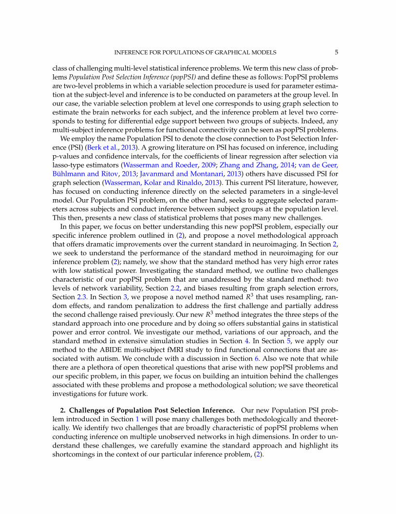
To understand the performance of this standard method, we present a small preview ofour simulation study discussed later in Section 4. Briefly, we assume that each subject graphin group A follows a small-world structure on p = 50 nodes; in group B, there are in addition150 differential edges, meaning that πA

(k,l) = 1 and πB(k,l) = 1 for all differential edges, (k, l).

We generate data according to this model with T = 400 time points and nA = nB = 20subjects in each group. Figure 1 illustrates the results of this standard approach as well asour new procedure, R3, which we will introduce later in Section 3. Part (a) gives ROC curvesfor the number of false positives verses true positives as each sequential test is rejected; parts(b) and (c) give the adjacency confusion matrix illustrating where the true and false positiveas well as false negative edges are detected in the graph structure.

Our motivating simulation shows that the standard approach performs terribly in termsof both error control and statistical power. While the magnitude of the poor performanceof this approach may seem astonishing, the poor performance should come as no surprise:The inferential procedure (e.g. test statistics) of the standard approach assume a one-levelmodel that would be appropriate when the subject graphs are fixed and known or directlyobserved quantities. When these subject networks are unobserved, however, and must beestimated from finite data, these one-level test statistics are incorrect for our two-level prob-lem. Specifically for two-level problems, the variance of parameters estimated by incorrectlyassuming a one-level models is underestimated. For our problem, the extra source of vari-ability arises from the graph selection procedure; we discuss challenges associated with thissubsequently in Section 2.2. Incorrect variance estimates, however, are not the only problemwith the standard approach: A more subtle problem arises from the fact that the proclivi-ties of graph selection procedures for the Gaussian graphical model lead to biased estimatesof the edge proportions, πg. As discussed in Section 2.3 and seen in Fig 1, graph selectionfalse positives and false negatives do not occur at random throughout the network structure,leading to biased group level estimates.

Also, it is important to note that the standard approach corresponding to a one-level prob-lem would be appropriate if we were able to perfectly estimate the network structure for eachsubject as this is then the same as assuming the subject networks were directly observed. For


0 20 40 60 80 100 120 140 1600

50

100

150

# of False Positives

# o

f T

rue

Po

siti

ves

0 20 40 60 80 100 120 140 1600

0.1

0.2

0.3

0.4

0.5

0.6

0.7

0.8

0.9

1

% o

f T

rue

Po

siti

ves

R3 Standard TP=FP Line

(a) Small World (b) Standard (c) R3

Figure 1: Motivating simulation study comparing the standard approach to our proposedprocedure, R3, in terms of (a) ROC curves for sequentially rejected tests, and confusion adja-cency matrices along with observed true positive rate (TPR) and false discovery proportion(FDP) for (b) the standard method and (c) our approach. The standard method performspoorly in terms of both error control and statistical power.

typical fMRI data, however, this is unlikely to ever happen due to (i) the limited sample size,T, relative to p and (ii) the highly connected network structures typical of brain networks(Bullmore and Sporns, 2009); these are known to violate irrepresentable and incoherenceconditions that are necessary for perfect graph selection (Meinshausen and Bühlmann, 2006;Ravikumar et al., 2011; Cai, Liu and Luo, 2011).

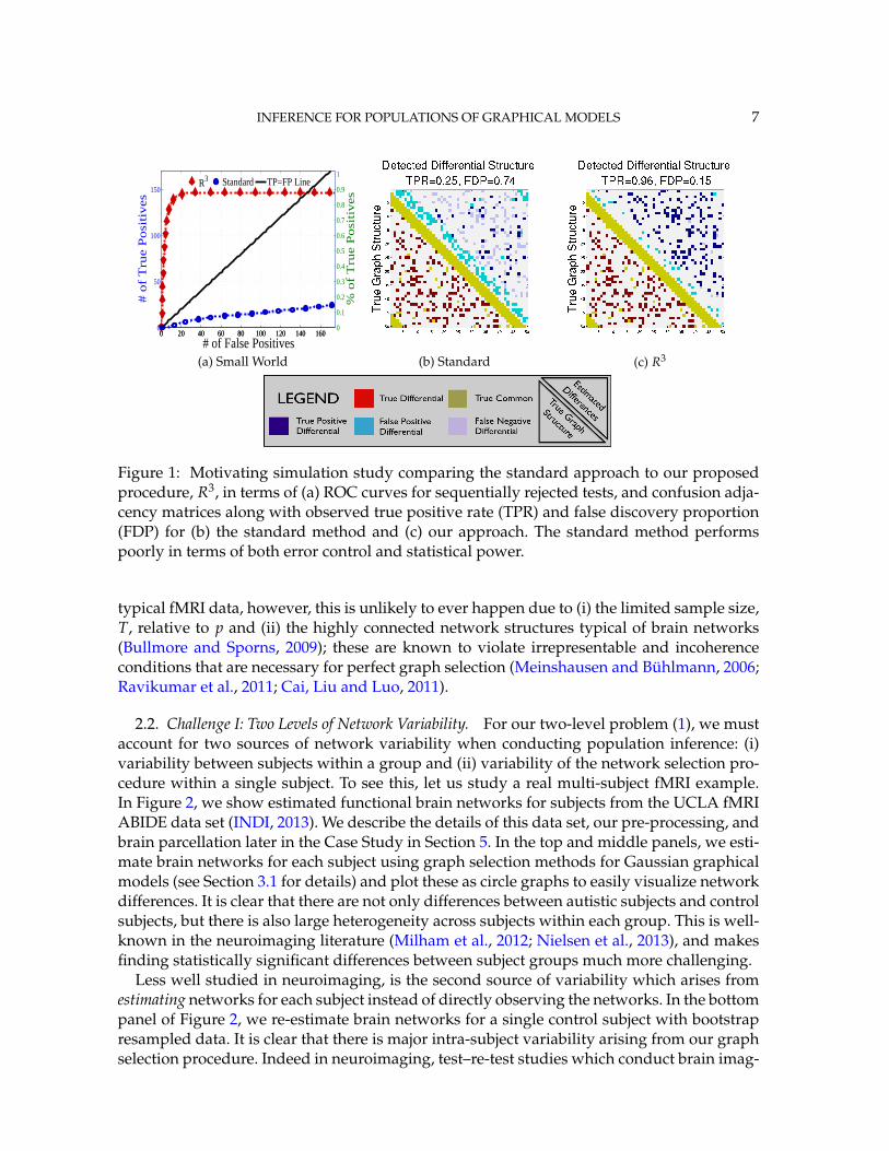
2.2. Challenge I: Two Levels of Network Variability. For our two-level problem (1), we mustaccount for two sources of network variability when conducting population inference: (i)variability between subjects within a group and (ii) variability of the network selection pro-cedure within a single subject. To see this, let us study a real multi-subject fMRI example.In Figure 2, we show estimated functional brain networks for subjects from the UCLA fMRIABIDE data set (INDI, 2013). We describe the details of this data set, our pre-processing, andbrain parcellation later in the Case Study in Section 5. In the top and middle panels, we esti-mate brain networks for each subject using graph selection methods for Gaussian graphicalmodels (see Section 3.1 for details) and plot these as circle graphs to easily visualize networkdifferences. It is clear that there are not only differences between autistic subjects and controlsubjects, but there is also large heterogeneity across subjects within each group. This is well-known in the neuroimaging literature (Milham et al., 2012; Nielsen et al., 2013), and makesfinding statistically significant differences between subject groups much more challenging.

Less well studied in neuroimaging, is the second source of variability which arises fromestimating networks for each subject instead of directly observing the networks. In the bottompanel of Figure 2, we re-estimate brain networks for a single control subject with bootstrapresampled data. It is clear that there is major intra-subject variability arising from our graphselection procedure. Indeed in neuroimaging, test–re-test studies which conduct brain imag-

8 NARAYAN ET AL.

(a) Autism Subject 1 (b) Autism Subject 2 (c) Autism Subject 3

(d) Control Subject 1 (e) Control Subject 2 (f) Control Subject 3

(g) Control 4, Resample 1 (h) Control 4, Resample 2 (i) Control 4, Resample 3

Figure 2: Motivating example of both inter- and intra-subject network variability in esti-mated functional brain networks. Gaussian graphical models were used to estimate net-works from the UCLA ABIDE fMRI data set (INDI, 2013) that we work with further in Sec-tion 5 for three autistic subjects (top), three control subjects (middle), and three bootstrapresampled data sets from a control subject (bottom). To conduct population inference acrosstwo groups, we must account for both the network variability between subjects (top andmiddle panels) as well as the variability associated with network estimation within a singlesubject (bottom panel). This also motivates the applicability of our two-level model, (1), forpopulation network inference.


ing on the same subject in repeated sessions have shown high variability in the subject’sestimated brain networks (Wang et al., 2011). This also motivates the necessity of using atwo-level model like (1) for population network inference as opposed to the one-level modeland test statistics of the standard procedure.

Now, let us consider the consequences of these two levels of network variability for ourspecific model and edge testing problem. Studying the variability via the post selection dis-tribution of the estimated networks, Θ(i), is a major challenge that has not yet been tackledin the statistics literature. Thus, a direct approach to conducting population inference for themodel (1) is beyond the scope of this paper and something that is saved for future work.Instead, we opt to break this problem into a series of simpler ones in an approach that ismore closely aligned with the standard procedure: We consider a separate two-level modelfor each edge in the network that can capture the two sources of network variability.

To model the two sources of network variability for each edge, we turn to the commonlyused Beta-Binomial model (Searle, Casella and McCulloch, 2009). As presented earlier, letY(i)

k,l = I(θ(i)k,l 6= 0) denote the edge support statistic for the (k, l)th edge associated with the

ith subject graphical parameter (precision matrix) Θ(i). Since each estimated network is arandom variable, Y(i)

k,l is a random variable whose variability is related to the selection vari-

ability of our estimated network for subject i. Let µ(i)(k,l) = P(θ

(i)(k,l) 6= 0) be a new parameter

denoting this subject-level probability of observing an edge at (k, l) in the ith subject; wemodel the selection variability in the ith subject as Y(i)

k,l ∼ Bern(µ(i)(k,l)). But, the edge selection

probabilities for each subject are themselves random variables related to the group-levelprobabilities for each edge. A common model for such probabilities is the beta distribution;thus, we let µ

(i)(k,l) ∼ Beta(αg

(k,l), βg(k,l)). Typically, a reparameterization of this model is used

where πg(k,l) = α

g(k,l)/(α

g(k,l) + β

g(k,l)) denotes the mean, E(µ

(i)(k,l)) = πg, of the Beta distribu-

tion, and where ρg(k,l) = 1/(αg

(k,l) + βg(k,l) + 1) is related to the variance of the Beta distribution

given by Var(µ(i)(k,l)) = ρ

g(k,l)π

g(k,l)(1− π

g(k,l)) (Searle, Casella and McCulloch, 2009). Suppose

we also observe m iid observations from this model and let Z(i)(k,l) = ∑m

j=1 Y(i)j,(k,l). Then, we

arrive at the familiar form of the Beta-Binomial model:

Z(i)(k,l)|µ

(i)(k,l)

iid∼ Bin(µ(i)(k,l), m), µ

(i)(k,l)

iid∼ Beta(π(g)(k,l), ρ

(g)(k,l)).(3)

This Beta-Binomial model, which is often used to model over-dispersed binary data, isideal for modeling both the intra-subject selection variability and the inter-subject group-level variabilities of each edge. To see this, consider the unconditional variance of Z(i)

(k,l)which incorporates two levels of variability as follows (for convenience, we suppress theedge indices):

Var(Z(i)) = ∑j

Var(Y(i)j ) + ∑

j<j′Cov(Y(i)

j , Y(i)j′ )

= mπg(1− πg) + m(m− 1)ρgπg(1− πg)︸︷︷︸Additional Binomial Variation

.(4)

Hence, the first term represents variability across subjects in group g and the second termrepresents the variability associated with the selection procedure within subject i, a quantity

10 NARAYAN ET AL.

that we assume to be constant across subjects i in each group g. Consider now what hap-pens if our true model follows this two-level Beta-Binomial model, but as with the standardapproach, we use a one-level Binomial model and associated two-sample test statistic. Thevariance is thus underestimated and the test statistic is overoptimistic. Then, when infer-ence is conducted for the population mean πg, using the incorrect Binomial model leads toinflated Type I error rates; this behavior has been well-documented (Weil, 1970; Liang andHanfelt, 1994). Hence, failure to use the correct two-level model which accounts for the twolevels of network variability partially explains the high error rates of the standard procedureobserved in Figure 1.

Notice in (3) that we have defined our Beta-Binomial model for the edge selection proba-bilities assuming that we have multiple iid observations from this model. For real fMRI data,we typically only have one scanning session per subject and hence only one estimate of thefunctional connectivity network, Θ(i), per subject. Then with only one observation, Y(i)

(k,l),for each subject, the Beta-Binomial model for each edge reduces to a Beta-Bernoulli model.In this model, the correlation parameter, ρg, is unidentifiable and the intra-subject variabil-ity associated with graph selection cannot be estimated. Thus, estimating the two-levels ofnetwork variability from data with only one observation is a challenge; in Section 3.2, wediscuss how we address this by using resampling techniques to estimate the second sourceof network variability.

2.3. Challenge II: Graph Selection Errors. In the previous section, we deconstructed ourproblem into a two-level model for each edge to simplify modeling the two sources of vari-ability. The models for each edge, however, are clearly not independent as we are modelingthe network support for a population of Gaussian graphical models. Here, we discuss howdependencies in the population network structure can lead to graph selection errors thatbias the estimates of our group-level edge parameters. These in turn lead to false positivesand false negatives when conducting inference at the group level.

Note that as previously discussed, we are working under the regime where we cannotobtain perfect estimates of the network support, as this is the most realistic scenario forreal fMRI data. Thus, it is constructive to understand the conditions under which perfectnetwork recovery or graph selection consistency is achievable so that we can understandthe consequences when these conditions are violated. Meinshausen and Bühlmann (2006)first introduced an irrepresentable condition for neighborhood selection-based estimationof GGMs that closely follows from irrepresentable or incoherence conditions for the lassoregression problem Zhao and Yu (2006). Later, Ravikumar et al. (2011) characterized a log-determinant based irrepresentable condition corresponding to estimating GGMs via penal-ized maximum likelihood, or the so-called graphical lasso method (Rothman et al., 2008;Friedman, Hastie and Tibshirani, 2008). This condition places restrictions on the Fisher in-formation matrix, Γ = Θ−1 ⊗ Θ−1; that is, if we let S denote the network support and letSC denote the non-support, then the condition requires that ‖|ΓT

Sc,S (ΓS,S)−1 |‖∞ ≤ 1 − η,

for some 0 < η < 1. In addition to irrepresentability conditions, the eigenvalues of the re-stricted Fisher information (ΓS,S)

−1 as well as covariance matrix(Θ−1)

S need to be boundedaway from zero, and the entries of the precision matrix Θi

(k,l) need to satisfy signal strengthconditions in order to prevent false exclusions of edges in each subject (Ravikumar et al.,2011). Both neighborhood and log-determinant irrepresentable conditions limit the amountof correlation within true edges and between true edges and non-edges; this, then places


severe restrictions on the model space and types of network structures where graph selec-tion consistency is achievable. As illustrated in Meinshausen (2008), certain simple networkstructures nearly guarantee irrepresentable conditions are violated in the population ver-sion, and consequently in finite samples. For example, estimators have a high probability ofincorrectly selecting an edge connecting two nodes that share similar node-neighborhoods.Now, let us return to our problem of conducting group level inference in situations wherewe know that the irrepresentable-type conditions are violated. Differentially present edgesin one group of subjects can change the network structure in a manner that graph selectionerrors are more likely to occur in one group. Thus, these group-level estimates will be biased.Following our procedure, biased group-level edge probability estimates will then bias teststatistics and lead to a higher probability of false positives or false negatives for group-levelinference.

To better understand this, we offer a small illustration in Figure 3. For simplicity, we as-sume that that the group-level probabilities for each edge in (1) are {0, 1}, meaning thatwe assume all subjects within a group share the same network structure. First in the leftpanel or Figure 3 (a), we assume that all subjects in the population share the common edgesin black, but that subjects in group two have a differentially present edge connecting (1,2).Since nodes 1 and 2 share common node-neighborhoods, an edge between (1,2) is selectedwith high probability in both group 1 and group 2 subjects. The group 1 estimate of edgeprobability (1,2) will then be biased and lead to a false negative when conducting inferenceacross the groups. Similarly in the left panel of Figure 3 (b), all subjects in group two havean additional differential edge connecting (2,5). Unlike in group 1, when (2,5) are connectedin group 2, nodes 4 and 5 are also highly correlated due to common node neighborhoods.Thus graph selection in group 2 will estimate an edge at (4,5) with high-probability, whereasgraph selection will be more likely to estimate the correct network in group 1. This resultsin a biased estimate for edge (4,5) in group two, leading to a false positive at (4,5) whenconducting inference at the group level. Thus even for simple graph structures, the locationof differentially present edges in the network structure can lead to graph selection errorsthat bias group-level estimates and lead to false positives and false negatives for group-levelinference. With more complicated network structures, this problem will be further exacer-bated.

In general, group-level biases in the edge probability estimates will occur when graph se-lection consistency does not hold for each subject. It is then difficult to control the overallerror rates of any inferential procedure at the group level. Analogous to standard irrepre-sentability conditions, we conjecture that there exists irrepresentability-like conditions forour problem (2), that limit the correlation between differential and non-differential edgesof the graph. That is, differentially present edges cannot be too correlated with commonedges (as illustrated in Figure 3 (a)) and differentially present edges cannot be too correlatedwith non-edges (as illustrated in Figure 3 (b)). While proving such conditions is beyond thescope of this paper, we explore these empirically in Section 4. Note that as we expect largeviolations of irrepresentable-like conditions with real fMRI data, it may be unrealistic to ex-pect that this problem can be fully solved and error rates properly controlled. However, wewould expect that any method that weakens irrepresentability conditions for graph estima-tion at the subject level will ameliorate biases in group-level edge estimates and lead to aninferential procedure with both higher statistical power and a lower false positive rate.

12 NARAYAN ET AL.

(a) Group-Level False Negative at (1,2). (b) Group-Level False Positive at (4,5).

Figure 3: Illustration of group level biases stemming from graph selection errors that wouldresult in false negatives (a) and false positives (b) for group inference. In each figure, truegraphs for a simple 5-node network are given on the left and estimated graphs on the right.In (a), an edge is likely to be selected at (1,2) in group one, resulting in a bias that would yielda false negative at the group-level. In (b), an edge is likely to be selected at (4,5) in group two,resulting in a bias that would yield a false positive at the group-level.

3. The R3 Method. We develop a novel procedure to conduct two-sample inference forour problem (2), namely, testing for the differential presence / absence of edges across a pop-ulation of networks. Our approach integrates the network estimation and inference prob-lems to address the two popPSI challenges outlined in Section 2. To achieve this, we employthree key ingredients - resampling, random penalization, and random effects; hence we callour procedure R3.

In this section, we briefly discuss each of the components of the R3 procedure separatelybefore putting them all together in Section 3.5. As discussed in Section 2.2, we use two levelmodels at the edge level to account for estimation variability as well as between subjectvariability of networks. However, we only observe one network per subject. In the absenceof multiple networks per subject, we use bootstrap resampling to generate network repli-cates for each subject, Section 3.2. We then use a beta-binomial model to model the two-leveledge probabilities and employ a beta-binomial two-sample random effects test statistic toaggregate our edge statistics over the two levels, Section 3.4. Thus, the resampling plus ran-dom effects portion of our procedure solves the first popPSI challenge. The second popPSIchallenge of graph selection errors that bias edge probability estimates is more difficult todirectly solve. We can dramatically ameliorate the affect of these errors, however, by us-ing a technique introduced by Meinshausen and Buhlmann (2010) - random regularizationpenalties, discussed in Section 3.3. Random penalties in conjunction with our resamplingprocedure thus address the second popPSI challenge. As subject-level network estimation isintegral to the entire R3 procedure, we begin by discussing how we estimate each functionalbrain network.

3.1. Preliminaries: Subject Graph Estimation. Our proposed R3 framework is compatiblewith any graph selection procedure for Gaussian graphical models. A popular method forestimating inverse covariances is the so-called graphical lasso or penalized maximum likeli-hood method, (d’Aspremont, Banerjee and El Ghaoui, 2006; Friedman, Hastie and Tibshi-


rani, 2008), which solves the following objective:

Θiλi(X(i)) = arg min

Θ�0L(Σi; Θ) + λi‖Θ‖1,off = arg min

Θ�0Tr(ΣiΘ)− log det(Θ) + λi‖Θ‖1,off

(5)

where Σi is the empirical sample covariance, Σi = 1T (X(i)TX(i)) and ‖Θ‖1,off = ∑k<l |θk,l |

is the `1 penalty on off-diagonals. Other estimation procedures such as the neighborhoodselection of Meinshausen and Bühlmann (2006) or the CLIME estimator of Cai, Liu and Luo(2011) could also be employed. In this paper, we obtain Θ using the QuIC implementationby Hsieh, Sustik and Ravikumar (2011). From hereon, we denote the presence of the (k, l)edge, selected by any graph estimation procedure as:

Yi(k,l)|Θ

(i)λi ,(k,l)(X(i)) = I(Θ(i)

λi ,(k,l)(X(i)) 6= 0)(6)

While inverse covariance estimation assumes that Xi consists of independent observationsfrom the multivariate normal, resting-state fMRI data consists of dependent observations.Thus, neuroimaging data effectively consists of fewer than T independent observations andis often well-described by an autoregressive process (Worsley et al., 2002). Hence, we firstuse an autoregressive model to whiten the time series and the Llung-Box test to verify thatwhitened observations are independent before applying graph selection procedures.

Notice, that we also need to estimate the regularization parameter, λi, controlling thegraph sparsity for each subject. In the standard approach, sparsity levels are typically fixedacross all subject networks (Bullmore and Sporns, 2009). As our procedure tests for differen-tial sparsity, however, we cannot enforce identical graph sparsity for each subject. Hence, weneed a good initial estimate of λi. While there are several model selection procedures pro-posed for graph selection, we employ the StARS procedure of (Liu, Roeder and Wasserman,2010).

3.2. R3: Resampling. Recall that, as discussed in Section 2.2, one of the challenges withpopPSI is accounting for two-levels of network variability when we typically obtain onlyone network estimate per subject. We address this by using resampling, specifically boot-strapping (Efron and Tibshirani, 1993), to obtain both a better estimate of the network andits variability. We also note that as we discuss in the next section, resampling will also becritical in addressing the second popPSI challenge.

For each subject i, we sample T out of T observations with replacement yielding thebootstrapped data, X∗b,(i). We then apply a graph selection procedure to this bootstrappeddata which gives us the bootstrapped edge selection statistic Y∗b,i

(k,l)|Θ∗b,(i)λi ,(k,l)(X∗b,(i)). While we

could estimate the edge-level probability for each subject by µ(i)(k,l) = Yi

(k,l), we could also use

bootstrap aggregation (Breiman, 1996) yielding µ(i)(k,l) ==

1B

B

∑b=1

Y∗b,i(k,l). Many have recently

shown the benefits of using resampling for graph selection with error control (Bach, 2008;Meinshausen and Buhlmann, 2010; Li et al., 2011; Liu, Roeder and Wasserman, 2010). Thus,we prefer the resampled statistic µi to µ(i). Although we cannot expect our estimate to be un-biased for µi

(k,l) in high-dimensional settings or for highly connected network structures (asdiscussed in Section 2.3), Meinshausen and Buhlmann (2010) and Shah and Samworth (2013)have shown that stability based statistics more effectively separate true and false edges. For

14 NARAYAN ET AL.

our R3 procedure, we will use resampling to not only improve estimation of edge selectionprobabilities, but also to estimate variability for two-level random effects models and withrandom penalization procedures as discussed subsequently.

3.3. R3: Random Penalization. As discussed in Section 2.3, graph selection errors can biasestimates of edge selection probabilities which in turn lead to errors when conducting infer-ence at the group level. For real fMRI data with limited samples T and highly connected net-work structures that violate irrepresentable-type conditions, we will likely never be able tofully solve the problems induced by graph selection errors. Here, we try to ameliorate theiraffect by employing random penalization techniques recently introduced by Meinshausenand Buhlmann (2010). For each bootstrap sample b = 1, . . . , B, we generate a p × p sym-metric matrix of regularization parameters that randomly penalizes each edge, denoted Λbi.We employ random penalization that modifies the objective, (5), through an element-wiseweighted penalty:

ΘiΛbi = arg min

Θ�0

(−2L(Σbi, Θ) + ‖Λbi ◦Θ‖1

)(7)

where ◦ is the element-wise Hadamard product. Our matrix of random penalties, Λbi, isobtained by perturbing the initial pilot estimate of the regularization parameter for eachsubject, λi, as follows:

Λbikl = λi + c λi

maxWk,l ∀ k < l(8)

where Pr{Wk,l = ±1} = 12 , c ∈ (0, .5) is fixed as a small fraction, and λi

max is the regular-ization parameter for each subject that results in the fully sparse graph. Thus, our randomperturbation procedure can be seen to penalize each edge independently as λ ± cλmax; forour purposes, we have found that c = .25 performs well. Note that our random penaltiesare different than the conservative scheme proposed by Meinshausen and Buhlmann (2010)for the purpose of controlling false positive edge selection. Other alternatives such as usingc ∼ U(0, .5) are also possible, and are closely related to the procedure of Li et al. (2011) whoaggregate edge selection frequencies over a range of perturbations of λ.

Intuitively, our randomized regularization scheme decreases the influence of the inclusionor exclusion of any given edge on the selection of other edges. Thus, we expect our approachto improve the problems associated with graph selection discussed in Section 3.1. In fact,several have recently shown that restricted eigenvalue and irrepresentability-type condi-tions can be violated for the original data, but hold when aggregating selection over randompenalizations (Meinshausen and Buhlmann, 2010; Bühlmann, van de Geer and Van de Geer,2011). Hence, with random penalization, consistent graph selection can be achieved whiletolerating larger correlations between variables. For our popPSI problem, we expect thatrandom penalization will allow us to tolerate more correlation between differential edgesand common edges, and differential edges with non-edges. We empirically study this intu-ition through simulations in Section 4.

3.4. R3: Random Effects. Recall that in Section 2.2 we introduced a Beta-Binomial model,(3), to account for the two sources of network variability at the edge level. With only one es-timated network, however, estimating two levels of variability and fitting the Beta-Binomialmodel was not possible. Now, we can use our bootstrap resampled data to properly fit the


Beta-Binomial model and obtain the corresponding two-sample test statistics for each edge.For each subject i and each edge (k, l), we obtain B resampled edge statistics, Yb,i

(k,l). Sup-

pressing the edge indices for notational simplicity, we then have that Z∗,i = 1B ∑B

b=1 Yb,i isour statistic associated with the subject edge probability, µi. Hence, we can re-write the Beta-Binomial model given in (3) for our bootstrapped statistics:

Z∗,i|µ(i) iid∼ Bin(µ(i), B), µ(i) iid∼ Beta(π(g), ρ(g)).(9)

Recall that the Beta-Binomial model is often used for over-dispersed or group-correlatedbinary data (Crowder, 1978). Our bootstrapped edge statistics over the subjects certainlyfit this model as bootstrapping results in positively correlated statistics within each subject(Bickel, Götze and van Zwet, 2012). As previously noted, this model also nicely captures thevariability of edge support both within and between subjects.

We propose to fit our Beta-Binomial model via the widely used moment estimators for πand ρ (Kleinman, 1973). For estimation, assume that we will always have a balanced numberof bootstrap samples per subject. Then estimates for π and ρ as proposed by Kleinman (1973);Ridout, Demétrio and Firth (1999) are as follows:

πg =1

ng∑

i∈Gg

Z∗,i & ρg =B

B− 1∑i∈Gg

(πg − Z∗,i)2

πg(1− πg)(n1 − 1)− 1

B− 1.(10)

These estimators are consistent for π and ρ (Moore, 1986) and are asymptotically normal(Kleinman, 1973). For balanced data such as in our case, these estimators exhibit only mildloss of efficiency compared to more commonly used likelihood-based estimators (Kleinman,1973). We choose to employ these estimators, however, as they are very simple to computeand widely used when conducting inference on π as in our problem. Specifically for infer-ence on π, it is well-known in the teratological literature that failure to account for ρ resultsin inflated Type I error rates (Weil, 1970; Liang and Hanfelt, 1994), but this inference hasalso been shown to be robust to various estimators for ρ (Moore, 1986). Further, many haveshown that for balanced data as in our case, the moment estimators for π and ρ give empir-ical Type I error control when conducting inference on π (Ridout, Demétrio and Firth, 1999;Liang and Hanfelt, 1994; Liang and Self, 1996). Given this wide literature, we thus opt to usethe computationally simpler moment estimators (10) to fit our Beta-Binomial model.

With these estimators, we develop a two-sample Wald test statistic appropriate for ourhypothesis (2). To this end, we need an estimate of the sampling variance of πg. Followingfrom (4) and using our estimates of πg and ρg, we can easily see that an estimate of thevariance of πg is given by:

s2g =

πg(1− πg)

m(ng − 1)(1 + (m− 1)ρg).

Putting everything together, we then arrive at the following two-sample Wald test-statisticfor our problem (2):

T =πA − πB

se(πB − πB)=

πA − πB√s2

A(nA−1)nA

+s2

B(nB−1)nB

.(11)

16 NARAYAN ET AL.

Following from Kleinman (1973), this test statistic is asymptotically standard normal as nAand nB → ∞. In fMRI studies, however, our sample sizes are typically small. Thus, we favorcomparing our test statistic T to a permutation null distribution to obtain p-values (Janssen,1997; Nichols and Holmes, 2002).

Algorithm 1 R3 := Resampling, Random Penalization and Random Effects Procedure

1. For each subject, i = 1, . . . n, obtain pilot estimates of the regularization parameter λi.(Section 3.1)

2. RESAMPLING AND RANDOM PENALIZATION:For b = 1, . . . B:

(a) Bootstrap data yielding X∗i,b.

(b) Fit weighted graphical lasso using random penalty matrix in Eq. (8) givingΘ(X∗i,b). (Section 3.3)

(c) Record edge support statistics Y∗i,bk,l = I(θ∗,i,b(k,l) 6= 0).

End.3. EDGE FILTERING: Eliminate edges absent from both groups from consideration, giv-

ing the set EF for testing. (Section 3.5)4. INFERENCE:

For (k, l) ∈ EF:

i. Compute test statistics T(k,l) as in Eq. (11) (Section 3.4)ii. Calculate p-values using a permutation mull distribution for T(k,l).

End.

iii Correct for multiplicity via the Benjamini-Yekutieli procedure.

3.5. The R3 Procedure. Now, we are ready to put our whole R3 procedure together. Weoutline our procedure in Algorithm 1 for conducting inference on the differential presenceof all edges in a population of graphical models, (2). Note that testing all edges would re-sult in an ultra-large-scale inference problem as there would be (p

2) hypotheses tested. Thisis clearly ill-advised; especially so since for brain connectivity networks, we expect rathersparse networks meaning that most edges are absent from both population groups. Thus,we limit our consideration to only the edges that are present in at least one of the populationgroups:

E cF , {(k, l) : Z∗i,

(k,l) ≤ Bτ, ∀ i = 1, . . . , n}

We filter out all edges that have edge proportions less than τ for all subjects, leaving ourfiltered edge set, EF. Notice that filtering is agnostic to group membership and thus doesnot affect group-level inference. We suggest taking τ ∈ (.2, .5) which typically reduces thenumber of edges under consideration from thousands to hundreds for real fMRI data. Addi-tionally, we must correct for multiple testing. As our test statistics will be highly dependent,we suggest using the Benjamini-Yekutieli procedure (Benjamini and Yekutieli, 2001) whichcontrols the false discovery rate under arbitrary dependencies. Finally, we note that insteadof testing all edges, our procedure could also be used to test targeted hypotheses regardingspecific edges.


4. Simulation Studies. We study our R3 procedure through a series of simulations, show-ing that R3 substantially improves statistical power and error control for our popPSI prob-lem, (2). We will particularly study how our method and the standard approach addresseach of the challenges outlined in Section 2.

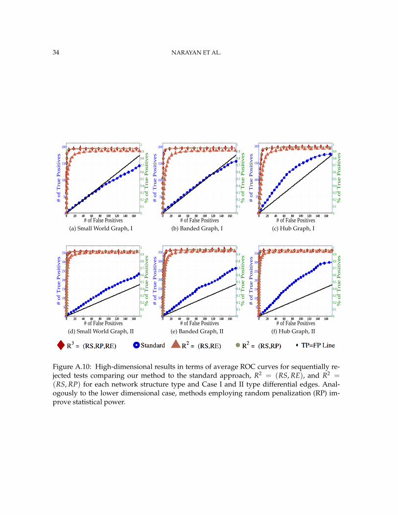
4.1. Simulation Setup. Henceforth, we will denote the components of R3 as Resampling(RS), Random Penalization (RP) and Random Effects (RE). To better understand how eachchallenge outlined in Section 2 as well as the our methodological solutions to these chal-lenges affect inferential procedures, we compare R3 not only to the standard approach butalso variations of our own method: R2 with (RS, RP) and R2 with (RS,RE). Recall from Sec-tion 2, that the standard approach uses two-sample test statistics associated with the one-level Binomial distribution. Both the numerator and denominator of this test statistic areincorrect, with the mean group level parameters biased by graph selection errors (ChallengeII in Section 2.3) and with the denominator under-estimating the variance components asso-ciated with two levels of network variability (Challenge I in Section 2.2). Our first variant,R2 = (RS, RP), seeks to address only Challenge II by ameliorating the bias in group-leveledge proportions using random penalization. Our second variant, R2 = (RS, RE) seeks toaddress only Challenge I by using the correct two-level Beta-Binomial model and test statis-tics. We adopt the same specifications outlined in Section 3.5 with λi selected using StARS(Liu, Roeder and Wasserman, 2010) for all methods. Methods including the RE componentuse random effect statistics from Section 3.4, while those without RE use the standard two-sample binomial proportions test as in Section 2.2. We control FDR at 10% for all methodsusing the Benjamini-Yekutieli approach (Benjamini and Yekutieli, 2001).

We study several simulation scenarios to fully test our methods. First, we generate mul-tivariate observations, X(i)

T×p, for each subject according to N (0, (Θ(i))−1). We simulate thestrength of connections for all edges as θi

(k,l) ∼ Uni f orm([−1.25,−1] ∪ [ 1, 1.25]), and

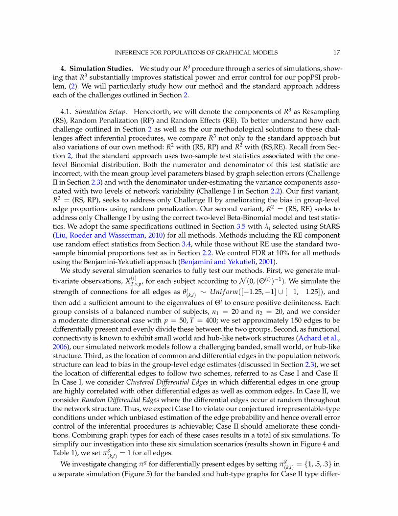
then add a sufficient amount to the eigenvalues of Θi to ensure positive definiteness. Eachgroup consists of a balanced number of subjects, n1 = 20 and n2 = 20, and we considera moderate dimensional case with p = 50, T = 400; we set approximately 150 edges to bedifferentially present and evenly divide these between the two groups. Second, as functionalconnectivity is known to exhibit small world and hub-like network structures (Achard et al.,2006), our simulated network models follow a challenging banded, small world, or hub-likestructure. Third, as the location of common and differential edges in the population networkstructure can lead to bias in the group-level edge estimates (discussed in Section 2.3), we setthe location of differential edges to follow two schemes, referred to as Case I and Case II.In Case I, we consider Clustered Differential Edges in which differential edges in one groupare highly correlated with other differential edges as well as common edges. In Case II, weconsider Random Differential Edges where the differential edges occur at random throughoutthe network structure. Thus, we expect Case I to violate our conjectured irrepresentable-typeconditions under which unbiased estimation of the edge probability and hence overall errorcontrol of the inferential procedures is achievable; Case II should ameliorate these condi-tions. Combining graph types for each of these cases results in a total of six simulations. Tosimplify our investigation into these six simulation scenarios (results shown in Figure 4 andTable 1), we set π

g(k,l) = 1 for all edges.

We investigate changing πg for differentially present edges by setting πg(k,l) = {1, .5, .3} in

a separate simulation (Figure 5) for the banded and hub-type graphs for Case II type differ-

18 NARAYAN ET AL.

0 20 40 60 80 100 120 140 1600

50

100


# o

f T

rue P

osi

tiv

es

0 20 40 60 80 100 120 140 1600

0.1

0.2

0.3

0.4

0.5

0.6

0.7

0.8

0.9

1

% o

f T

rue P

osi

tiv

es

(a) Small World Graph, I

0 20 40 60 80 100 120 140 1600

50

100

150

# of False Positives#

of

Tru

e P

osi

tiv

es

0 20 40 60 80 100 120 140 1600

0.1

0.2

0.3

0.4

0.5

0.6

0.7

0.8

0.9

1

% o

f T

rue P

osi

tiv

es

(b) Banded Graph, I

0 20 40 60 80 100 120 140 1600

50

100


# o

f T

rue P

osi

tiv

es

0 20 40 60 80 100 120 140 1600

0.1

0.2

0.3

0.4

0.5

0.6

0.7

0.8

0.9

1

% o

f T

rue P

osi

tiv

es

(c) Hub Graph, I

0 20 40 60 80 100 120 140 1600

50

100

150


# o

f T

rue P

osi

tiv

es

0 20 40 60 80 100 120 140 1600

0.1

0.2

0.3

0.4

0.5

0.6

0.7

0.8

0.9

1

% o

f T

rue P

osi

tiv

es

(d) Small World Graph, II

0 20 40 60 80 100 120 140 1600

50

100

150


# o

f T

rue P

osi

tiv

es

0 20 40 60 80 100 120 140 1600

0.1

0.2

0.3

0.4

0.5

0.6

0.7

0.8

0.9

1

% o

f T

rue P

osi

tiv

es

(e) Banded Graph, II

0 20 40 60 80 100 120 140 1600

50

100

150


of

Tru

e P

osi

tiv

es

0 20 40 60 80 100 120 140 1600

0.1

0.2

0.3

0.4

0.5

0.6

0.7

0.8

0.9

1

% o

f T

rue P

osi

tiv

es

(f) Hub Graph, II

Figure 4: Average ROC curves for sequentially rejected tests comparing our method to thestandard approach, R2 = (RS, RE), and R2 = (RS, RP) for each network structure type andCase I and II type differential edges. Methods employing random penalization (RP) improvestatistical power as they ameliorate graph selection errors that bias group-level estimates.

ential edges. For this simulation, we use population correlations rather than covariances inorder to eliminate variations in scale across subjects. Additionally for fair comparisons here,we limit the number of differential edges to 25 per group and fix the degree of the commonsupport to be 0.12p.

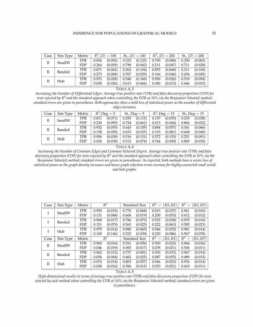
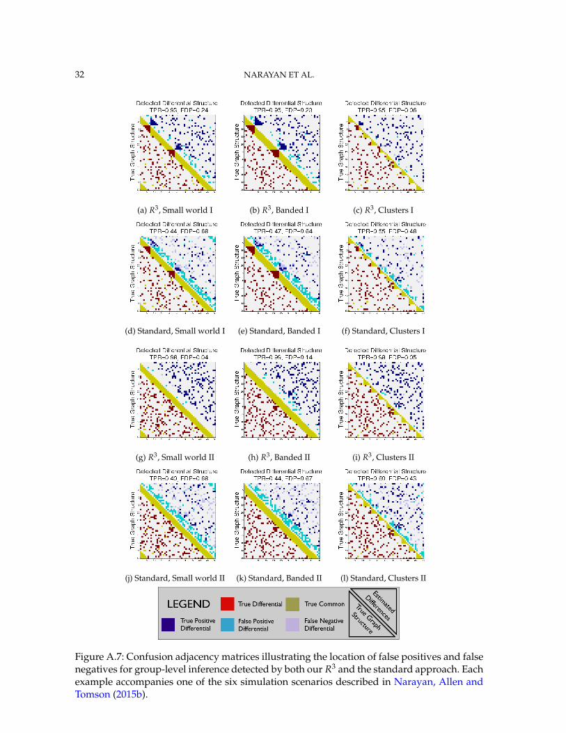
Further simulations studies as well as additional supporting material for our simulationscan be found in the supplementary materials (Narayan, Allen and Tomson, 2015a). Theseinclude confusion adjacency matrices showing the location of false positives and false neg-atives in the network structure for all methods, an analogous simulation study in a high-dimensional setting p > T, and a study of the impact of graph sparsity for both commonand differential edges on our methods.

4.2. Results. In Figure 4 and Table 1, we present our main simulation results compar-ing R3 to the two variations of our R2 method and the standard approach for three net-work structures and Case I and II type differential edges. First for Figure 4, we report resultsin terms of operating characteristics averaged across 50 replicates with the number of true


Case Sim Type Metric R3 Standard Test R2 = (RS, RE) R2 = (RS, RP)

I SmallW TPR 0.934 (0.036) 0.542 (0.096) 0.739 (0.082) 0.937 (0.037)FDP 0.245 (0.079) 0.661 (0.028) 0.476 (0.040) 0.643 (0.016)

I Banded TPR 0.921 (0.069) 0.524 (0.105) 0.735 (0.091) 0.933 (0.038)FDP 0.261 (0.122) 0.645 (0.039) 0.446 (0.053) 0.624 (0.041)

I Hub TPR 0.967 (0.021) 0.616 (0.131) 0.763 (0.099) 0.968 (0.021)FDP 0.107 (0.056) 0.497 (0.040) 0.306 (0.048) 0.474 (0.019)


II SmallW TPR 0.959 (0.026) 0.483 (0.097) 0.792 (0.071) 0.959 (0.026)FDP 0.112 (0.079) 0.659 (0.042) 0.370 (0.037) 0.615 (0.012)

II Banded TPR 0.941 (0.044) 0.450 (0.105) 0.724 (0.105) 0.946 (0.043)FDP 0.199 (0.095) 0.667 (0.042) 0.425 (0.058) 0.623 (0.018)

II Hub TPR 0.971 (0.023) 0.533 (0.133) 0.735 (0.106) 0.972 (0.023)FDP 0.051 (0.029) 0.463 (0.046) 0.262 (0.042) 0.406 (0.009)

TABLE 1Average true positive rate (TPR) and false discovery proportion (FDP) for tests rejected by each method when controlling

the FDR at 10% via the Benjamini-Yekutieli method; standard errors are given in parentheses. Methods employingrandom effects models and test statistics yield improved Type I error rates.

0 500

50


# of

Tru

e P

ositi

ves

0

0.25

0.5

0.75

1

% o

f T

rue

Posi

tives

(a) Banded Graph, II

0 500

50


# of

Tru

e P

ositi

ves

0

0.25

0.5

0.75

1

% o

f T

rue

Posi

tives

R3, π=1

St., π=1

R3, π=.5

St., π=.5

R3, π=.3

St., π=.3

(b) Hub Graph, II

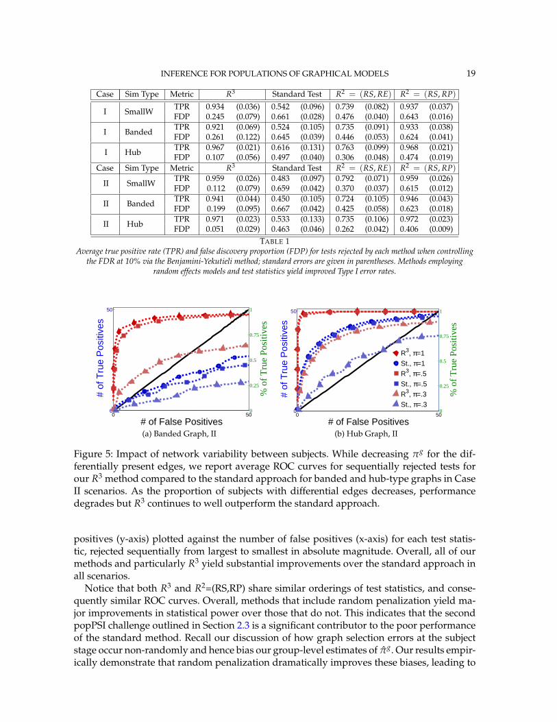
Figure 5: Impact of network variability between subjects. While decreasing πg for the dif-ferentially present edges, we report average ROC curves for sequentially rejected tests forour R3 method compared to the standard approach for banded and hub-type graphs in CaseII scenarios. As the proportion of subjects with differential edges decreases, performancedegrades but R3 continues to well outperform the standard approach.

positives (y-axis) plotted against the number of false positives (x-axis) for each test statis-tic, rejected sequentially from largest to smallest in absolute magnitude. Overall, all of ourmethods and particularly R3 yield substantial improvements over the standard approach inall scenarios.

Notice that both R3 and R2=(RS,RP) share similar orderings of test statistics, and conse-quently similar ROC curves. Overall, methods that include random penalization yield ma-jor improvements in statistical power over those that do not. This indicates that the secondpopPSI challenge outlined in Section 2.3 is a significant contributor to the poor performanceof the standard method. Recall our discussion of how graph selection errors at the subjectstage occur non-randomly and hence bias our group-level estimates of πg. Our results empir-ically demonstrate that random penalization dramatically improves these biases, leading to

20 NARAYAN ET AL.

less bias in our test statistics and hence improvements in both Type I and Type II error rates.Furthermore, in Case II scenarios where selection errors are moderate, the performance gapbetween any method containing RP over R2 = (RS, RE) reduces compared to Case I sce-narios where selection errors are more severe. Thus, the benefits of random penalization aregreater when selection errors are more abundant. Confusion adjacency matrices illustrat-ing the location of inferential errors for our methods shown in the supplemental materialsalso indicate that random penalization improves graph selection in cases where there arelarger correlations between differential edges and common edges. Similar results hold forour high-dimensional study presented in the supplemental material.

Table 1, which accompanies Figure 4, gives the empirical true positive and false discov-ery rates (FDR) averaged over 50 simulation replicates when the Benjamini-Yekutieli (Ben-jamini and Yekutieli, 2001) procedure controlling the FDR at 10% is used to determine thenumber of tests to reject. First, notice that the observed false discovery proportion (FDP) ofour R3 procedure is not 10% on average, indicating that our method does not fully controlthe FDR. This occurs because we specifically simulate difficult and realistic fMRI scenar-ios with graph structures that severely violate irrepresentable-type conditions. In situations(not shown) where irrepresentable-type conditions are met that ensure graph selection con-sistency, our procedure as well as the standard method correctly control the FDR. As dis-cussed in Section 2.3, in situations where graph selection errors occur with high probability,it is likely impossible to provably control the FDR, consistent with our empirical results. Yeteven though R3 does not fully control the FDR, our error rates are dramatically improvedover the standard approach and other variations of our procedure.

Also in Table 1, observe that R2 =(RS,RP), which had similarly ordered test statistics toR3, has dramatically worse Type I error rates that do not come close to controlling the FDR.While R2 =(RS,RE) also does not control the FDR, the error rates are much improved overR2 =(RS,RP). These results demonstrate that using two-level models with the correct ran-dom effects test statistics are crucial to Type I error control. Recall from Section 2.2, thatusing the one-level Binomial model leads to an under-estimation of the variance term whichin turn inflates test statistics and leads to an increase in false positives. Note also that theestimated FDP of R3 is still a major improvement over that of R2 =(RS,RE). This occurs asthe problem of graph selection errors induces both Type I and Type II errors. Hence, theseresults demonstrate the necessity of all three of our R3 ingredients. Finally, observe that ourerror rates in Case II scenarios are better than those for Case I scenarios, again indicatingthat differential edges that are highly correlated with non-edges and common edges poseparticular challenges for our popPSI problem. These results are also corroborated in ourhigh-dimensional study presented in the supplemental materials.

Lastly, in Figure 5, we study the effect of letting the network structure vary across subjectsby decreasing the differential group edge probability, πg. Our method continues to performwell for πg ∈ [.5 1]. However, when the differential edge probability drops further to πg = .3,we see that both R3 and the standard approach have greatly reduced statistical power, as onewould expect. Despite this, R3 continues to outperform the standard approach.

Overall, our results demonstrate the difficulty of solving the challenges associated withour popPSI problem. In particular, using the correct two-level models are critical to TypeI error control while solving or ameliorating the problem of graph selection errors at thesubject level are critical for both Type I and Type II error control. Our results also demonstratethe substantial outperformance of our new R3 method over existing state-of-the-art methodsin neuroimaging.


5. Case Study: Differential Functional Connections in Autism. We apply our R3 methodto identify differential functional connections associated with Autism Spectrum Disorders(ASD) in a publicly available fMRI study from the Autism Brain Imaging Data Exchange(ABIDE) (INDI, 2013) consortium.

5.1. fMRI data acquisition and preprocessing. We use resting state fMRI data from the UCLASample 1, (Rudie et al., 2012a; INDI, 2013) which consists of 73 subjects, with 32 controls and41 subjects diagnosed with Autism Spectrum Disorder (ASD) based on the ADOS or ADI-Rcriteria. In addition to no history of illness, the controls did not have a first degree relativewith autism. The fMRI scans from the UCLA site were acquired when the subjects werepassively at rest for 6 minutes using a Siemens 3 T Trio.(T2∗-weighted functional images:TR = 3000 ms, TE = 28 ms, matrix size 64× 64, 19.2 cm FoV, and 34 4-mm thick slices (nogap), interleaved acquisition, with an in-plane voxel dimension of 3.0× 3.0 mm). This re-sults in a total of 120 images per subject. We preprocess the data minimally using FMRIB’sSoftware Library (www.fmrib.ox.ac.uk/fsl). These steps include brain extraction, spatialsmoothing of the images using a Gaussian kernel with FWHM = 5mm, band-pass filtering(.01Hz < f < 0.1Hz) to eliminate respiratory and cardiovascular signals, and registering im-ages to standard MNI space. We parcellate the images using the anatomical Harvard-OxfordAtlas (Desikan et al., 2006) to obtain 113 regions of interest. We average all voxel time-serieswithin a region to obtain a single time-series per region. Thus, our final processed data ma-trix consists of 113 regions × 120 time points × 73 subjects.

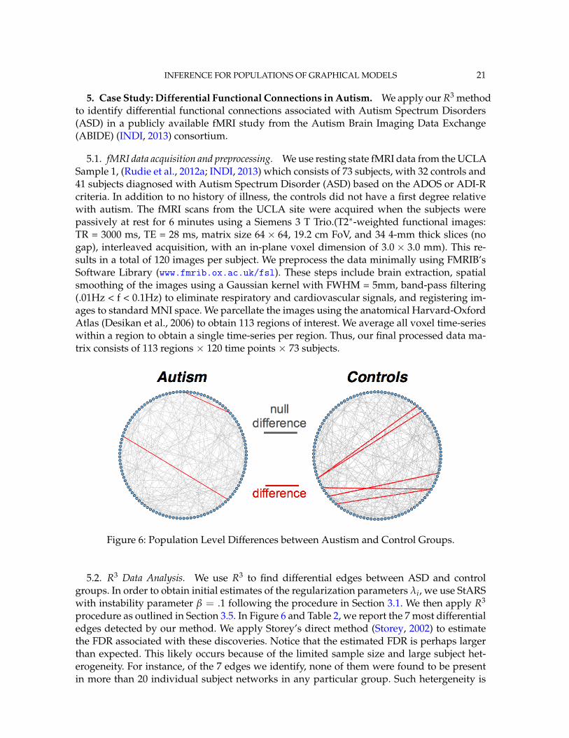
Figure 6: Population Level Differences between Austism and Control Groups.

5.2. R3 Data Analysis. We use R3 to find differential edges between ASD and controlgroups. In order to obtain initial estimates of the regularization parameters λi, we use StARSwith instability parameter β = .1 following the procedure in Section 3.1. We then apply R3

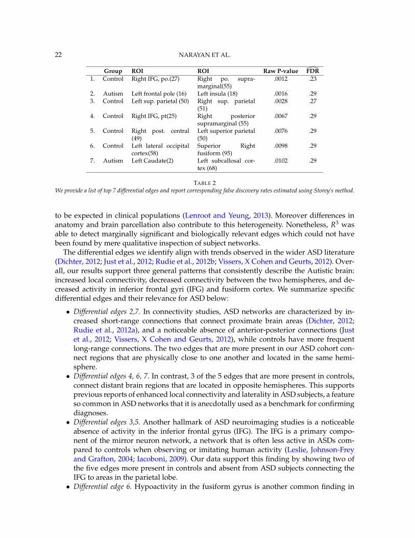
procedure as outlined in Section 3.5. In Figure 6 and Table 2, we report the 7 most differentialedges detected by our method. We apply Storey’s direct method (Storey, 2002) to estimatethe FDR associated with these discoveries. Notice that the estimated FDR is perhaps largerthan expected. This likely occurs because of the limited sample size and large subject het-erogeneity. For instance, of the 7 edges we identify, none of them were found to be presentin more than 20 individual subject networks in any particular group. Such hetergeneity is

www.fmrib.ox.ac.uk/fsl

22 NARAYAN ET AL.

Group ROI ROI Raw P-value FDR1. Control Right IFG, po.(27) Right po. supra-

marginal(55).0012 .23

2. Autism Left frontal pole (16) Left insula (18) .0016 .293. Control Left sup. parietal (50) Right sup. parietal

(51).0028 .27

4. Control Right IFG, pt(25) Right posteriorsupramarginal (55)

.0067 .29

5. Control Right post. central(49)

Left superior parietal(50)

.0076 .29

6. Control Left lateral occipitalcortex(58)

Superior Rightfusiform (95)

.0098 .29

7. Autism Left Caudate(2) Left subcallosal cor-tex (68)

.0102 .29

TABLE 2We provide a list of top 7 differential edges and report corresponding false discovery rates estimated using Storey’s method.

to be expected in clinical populations (Lenroot and Yeung, 2013). Moreover differences inanatomy and brain parcellation also contribute to this heterogeneity. Nonetheless, R3 wasable to detect marginally significant and biologically relevant edges which could not havebeen found by mere qualitative inspection of subject networks.

The differential edges we identify align with trends observed in the wider ASD literature(Dichter, 2012; Just et al., 2012; Rudie et al., 2012b; Vissers, X Cohen and Geurts, 2012). Over-all, our results support three general patterns that consistently describe the Autistic brain:increased local connectivity, decreased connectivity between the two hemispheres, and de-creased activity in inferior frontal gyri (IFG) and fusiform cortex. We summarize specificdifferential edges and their relevance for ASD below:

• Differential edges 2,7. In connectivity studies, ASD networks are characterized by in-creased short-range connections that connect proximate brain areas (Dichter, 2012;Rudie et al., 2012a), and a noticeable absence of anterior-posterior connections (Justet al., 2012; Vissers, X Cohen and Geurts, 2012), while controls have more frequentlong-range connections. The two edges that are more present in our ASD cohort con-nect regions that are physically close to one another and located in the same hemi-sphere.• Differential edges 4, 6, 7. In contrast, 3 of the 5 edges that are more present in controls,

connect distant brain regions that are located in opposite hemispheres. This supportsprevious reports of enhanced local connectivity and laterality in ASD subjects, a featureso common in ASD networks that it is anecdotally used as a benchmark for confirmingdiagnoses.• Differential edges 3,5. Another hallmark of ASD neuroimaging studies is a noticeable

absence of activity in the inferior frontal gyrus (IFG). The IFG is a primary compo-nent of the mirror neuron network, a network that is often less active in ASDs com-pared to controls when observing or imitating human activity (Leslie, Johnson-Freyand Grafton, 2004; Iacoboni, 2009). Our data support this finding by showing two ofthe five edges more present in controls and absent from ASD subjects connecting theIFG to areas in the parietal lobe.• Differential edge 6. Hypoactivity in the fusiform gyrus is another common finding in


ASD subjects compared to controls (Corbett et al., 2009; Pierce and Redcay, 2008). Ourresults suggest an edge between the right fusiform gyrus and the left lateral occipitalcortex that does not occur in ASD.

Our results corroborate a number of common trends in the ASD neuroimaging literature.However, since this is the first study to specifically investigate differential functional con-nections in ASD, we cannot validate the biological significance of edges we identified usingexisting literature. We plan to verify these findings using ABIDE data from alternative sitesas well as other independent ASD datasets.

6. Discussion. In this paper, we have studied a new statistical problem that arises whenconducting inference for multi-subject functional connectivity. Our problem assumes a two-level model where subject data arises from a Gaussian graphical model and the edge sup-port is governed by a group level probability, with inference conducted on these group levelparameters. This leads to a completely new class of statistical problems that we term Popu-lation Post Selection Inference (popPSI). In this paper, we have discussed some of the chal-lenges of our popPSI problem and proposed a new procedure that partially solves thesechallenges. As we work with a new class of inference problems, however, there are manyremaining questions and open areas of related research.

Our model and inference problem is similar in spirit to testing for differences in the el-ements of two covariance or inverse covariance matrices (Cai, Liu and Xia, 2013). If we letπA and πB only take values in {0, 1}, then in fact our problem perfectly coincides with thatof Zhao, Cai and Li (2014). Given this, some may argue that we needlessly complicate theproblem and potentially lose statistical power by using separate estimators for subject-levelnetworks instead of a joint group estimator. While this would certainly be true in the casewhere subjects within a group all follow the same distribution, there are a number of rea-sons why our approach is advantageous for real fMRI data: (1) Assuming that each subjectfollows a potentially different brain network model mimics assumptions for functional con-nectivity where neuroscientists expect each subject to have a slightly different brain network;this is especially true for resting-state data in which passive subjects may be thinking aboutdifferent items. (2) Our models and methods are more closely aligned with the goal of neu-roscientists who along with inference wish to examine each subject’s brain network and un-derstand the network differences between subjects both within a group and between groups.Estimating group networks does not permit this analysis across subjects. Most importantly,since group networks do not model between-subject variability, corresponding inferentialresults do not generalize to larger populations. (3) Our approach is also more robust to po-tential outliers and artifacts common in neuroimaging (Smith et al., 2011; Power et al., 2012).If a few subjects have gross artifacts or head motion, these can easily corrupt group-levelgraph estimation and hence group-level inference. By estimating separate graphs for eachsubject and testing the stability proportion of each edge, our procedure will be more robustto subject-level artifacts. (4) Our framework can easily be extended beyond the two-groupmodel to testing parameters for multiple groups or even for continuous clinical outcomes byusing linear and generalized linear mixed effects models and test statistics (Searle, Casellaand McCulloch, 2009). This is possible as we directly estimate separate subject networks andthe between and within network variability; testing group-level parameters directly cannoteasily be extended in this manner. Finally, as our approach can be seen as building upon thestandard approach in neuroimaging by incorporating resampling, random effects, and ran-

24 NARAYAN ET AL.

dom penalization, it is more likely to be adopted by neuroimagers than a new and unfamiliarparadigm.

This paper has focused on characterizing our particular popPSI problem, providing intu-ition as to why standard approaches in neuroimaging fail, and suggesting a methodologicalsolution. Studying this problem from a theoretical perspective is beyond the scope of thispaper and hence, many open theoretical questions remain. We seek to control the overallerror rate or FDR of the procedure; studying if this is achievable and under what theoreticalconditions is an important open problem. Based on our empirical investigations in Section 4and our discussion in Section 2.3, we conjecture that this is possible under extensions of anirrepresentable or incoherence condition. More specifically, these conditions limit the corre-lation between edges that are common across subjects and those that have differential edgeprobabilities, especially when such common and differential edges belong to the same con-nected component, as well as limit correlations between those that have differential edgeprobabilities and the non-edges. Another interesting line of theoretical investigation is re-lating the overall error rate of the inferential procedure to that of the error rate for graphselection at the subject level. Additionally, there are likely many interesting theoretical ques-tions that arise from characterizing and studying popPSI problems more generally beyondour specific model.

Our model and methods can be extended well beyond testing for the differential presenceof an edge in a population of Gaussian graphical models. In particular, our basic approach isapplicable to inference for any support related metric such as overall network sparsity or thedegree of each node. Here, one could assume the group level parameters follow a Poisson ornormal distribution and adjust our random effects Beta-Binomial estimators and test statis-tics accordingly. Also as mentioned above, we can extend our framework to test multiplegroups or continuous clinical outcomes by using linear and generalized linear mixed effectsmodels. Further, other network models such as a sparse covariance model could be used forthe subject networks.

For application to multi-subject fMRI data, there are also many other considerations anditems to investigate. In Section 1, we mentioned that data for each subject must be parcellatedinto a matrix of brain regions by time series. More investigations are needed to determinewhich parcellation method to use and how this affects network estimation and group-levelinference. Additionally, many have noted that resting state fMRI data is particularly sensi-tive to physiological artifacts such as head motion (Power et al., 2012); further studies arealso needed to determine how head motion affects group-level network inference. Finallywe note, that our inference paradigm can additionally be employed for task related fMRIexperiments as well as in Tomson et al. (2013).

While we introduce a new class of statistical problems, Population PSI, these problems ac-tually arise often in neuroimaging. First, the problems and challenges we outline for the stan-dard approach used for functional connectivity with fMRI data extend to many other formsof connectivity in neuroimaging. Consider structural connectivity which estimates networksbased on the number of tracts connecting different brain regions. These tracts, however, areestimated by complicated probabilistic tractography algorithms (Ciccarelli et al., 2003) fromdiffusion tensor imaging. Hence, estimates of subject-level networks are imperfect, resultingin two-levels of network variability and then a popPSI-type group level inference problem.Similar problems arise for vector autoregressive graphical models or effective connectiv-ity estimated from EEG, MEG, fMRI, or ECoG data. Additionally, popPSI problems arisein neuroimaging applications beyond network inference where a selection based statistical


learning procedure is applied at the subject level but inference is to be conducted across sub-jects. Finally, our work provides a cautionary tale about conducting inference on estimatedparameters without properly accounting for multiple levels of variability.

In conclusion, we have studied a new problem arising in inference for multi-subject con-nectivity. As with any new framework many open questions and directions for future re-search remain. Software for our R3 procedure will be available as part of the Markov Net-work Matlab Toolbox https://bitbucket.org/gastats/monet.

Acknowledgments. M.N. and G.A. are supported by NSF DMS 1209017 and 1264058;S.T. is supported by an NIH training grant 5T32NS048004-08; M.N. is supported by AmazonWeb Services (AWS) research grant for computational resources.

SUPPLEMENTARY MATERIAL

Supplement A: Supplementary Material to Two Sample Inference for Populations ofGraphical Models, with Applications to Functional Brain Connectivity(doi: arxiv.org/abs/0000.0000). Additional simulations demonstrate that R3 outperforms thestandard approach in high dimensional regimes and when increasing differential or commongraph density.

References.

ACHARD, S., SALVADOR, R., WHITCHER, B., SUCKLING, J. and BULLMORE, E. (2006). Aresilient, low-frequency, small-world human brain functional network with highly con-nected association cortical hubs. J. Neurosci. 26 63–72.

BACH, F. R. (2008). Bolasso: model consistent lasso estimation through the bootstrap. InProceedings of the 25th International Conference on Machine learning 33–40. ACM.

BALACHANDRAN, P., AIROLDI, E. and KOLACZYK, E. (2013). Inference of Network Sum-mary Statistics Through Network Denoising. arXiv preprint arXiv:1310.0423.

BECKMANN, C. F., JENKINSON, M. and SMITH, S. M. (2003). General multilevel linear mod-eling for group analysis in FMRI. Neuroimage 20 1052–1063.

BENJAMINI, Y. and YEKUTIELI, D. (2001). The control of the false discovery rate in multipletesting under dependency. Ann. Statist. 29 1165–1188. MR1869245 (2002i:62135)

BERK, R., BROWN, L., BUJA, A., ZHANG, K. and ZHAO, L. (2013). Valid post-selection in-ference. Ann. Stat.

BICKEL, P. J., GÖTZE, F. and VAN ZWET, W. R. (2012). Resampling fewer than n observations:gains, losses, and remedies for losses. Springer.

BREIMAN, L. (1996). Heuristics of instability and stabilization in model selection. The annalsof statistics 24 2350–2383.

BÜHLMANN, P. L., VAN DE GEER, S. A. and VAN DE GEER, S. (2011). Statistics for high-dimensional data. Springer.

BULLMORE, E. (2012). Functional network endophenotypes of psychotic disorders. Biol. Psy-chiatry 71 844.

BULLMORE, E. and SPORNS, O. (2009). Complex brain networks: graph theoretical analysisof structural and functional systems. Nat Rev Neurosci 10 186–198.

CAI, T., LIU, W. and LUO, X. (2011). A constrained `1 minimization approach to sparseprecision matrix estimation. JASA 106 594–607.

CAI, T., LIU, W. and XIA, Y. (2013). Two-sample covariance matrix testing and support re-covery in high-dimensional and sparse settings. JASA 108 265–277.

https://bitbucket.org/gastats/monet

http://dx.doi.org/arxiv.org/abs/0000.0000

http://www.ams.org/mathscinet-getitem?mr=1869245

26 NARAYAN ET AL.

CICCARELLI, O., PARKER, G., TOOSY, A., WHEELER-KINGSHOTT, C., BARKER, G.,BOULBY, P., MILLER, D. and THOMPSON, A. (2003). From diffusion tractography toquantitative white matter tract measures: a reproducibility study. Neuroimage 18 348–359.

CORBETT, B. A., CARMEAN, V., RAVIZZA, S., WENDELKEN, C., HENRY, M. L., CARTER, C.and RIVERA, S. M. (2009). A functional and structural study of emotion and face pro-cessing in children with autism. Psychiatry Research: Neuroimaging 173 196–205.

CRADDOCK, R. C., JBABDI, S., YAN, C.-G., VOGELSTEIN, J. T., CASTELLANOS, F. X.,DI MARTINO, A., KELLY, C., HEBERLEIN, K., COLCOMBE, S. and MILHAM, M. P. (2013).Imaging human connectomes at the macroscale. Nature Methods 10 524–539.

CROWDER, M. J. (1978). Beta-binomial Anova for proportions. Applied Statistics 34–37.DANAHER, P., WANG, P. and WITTEN, D. M. (2011). The joint graphical lasso for inverse

covariance estimation across multiple classes. arXiv preprint arXiv:1111.0324.D’ASPREMONT, A., BANERJEE, O. and EL GHAOUI, L. (2006). First-order methods for sparse

covariance selection. ArXiv Mathematics e-prints.DICHTER, G. S. (2012). Functional magnetic resonance imaging of autism spectrum disor-

ders. Dialogues in clinical neuroscience 14 319.EFRON, B. and TIBSHIRANI, R. J. (1993). An Introduction to the Bootstrap. Chapman & Hall,

London, U.K.FISCHL, B., VAN DER KOUWE, A., DESTRIEUX, C., HALGREN, E., SÉGONNE, F.,

SALAT, D. H., BUSA, E., SEIDMAN, L. J., GOLDSTEIN, J., KENNEDY, D. et al. (2004).Automatically parcellating the human cerebral cortex. Cerebral cortex 14 11–22.

FRIEDMAN, J., HASTIE, T. and TIBSHIRANI, R. J. (2008). Sparse inverse covariance estima-tion with the graphical lasso. Biostatistics 9 432–441.

GUO, J., ELIZAVETA LEVINA, G. M. and ZHU, J. (2011). Joint Estimation of Multiple Graph-ical Models. Biometrika 98 1-15.

HSIEH, C.-J., SUSTIK, I. MÁTYÁS A. AND DHILLON and RAVIKUMAR, P. (2011). SparseInverse Covariance Matrix Estimation Using Quadratic Approximation. In Advancesin Neural Information Processing Systems 24 (J. Shawe-Taylor, R. S. Zemel, P. Bartlett,F. C. N. Pereira and K. Q. Weinberger, eds.) 2330–2338.

HUANG, S., LI, J., SUN, L., YE, J., FLEISHER, A., WU, T., CHEN, K. and REIMAN, E. (2010).Learning brain connectivity of Alzheimer’s disease by sparse inverse covariance esti-mation. NeuroImage 50 935-949.

IACOBONI, M. (2009). Imitation, empathy, and mirror neurons. Annual review of psychology60 653–670.

INDI (2013). ABIDE: Autism Brain Imaging Data Exchange.JANSSEN, A. (1997). Studentized permutation tests for non-i.i.d. hypotheses and the gener-

alized Behrens-Fisher problem. Statistics & Probability Letters 36 9-21.JAVANMARD, A. and MONTANARI, A. (2013). Confidence Intervals and Hypothesis Testing

for High-Dimensional Regression. arXiv preprint arXiv:1306.3171.JUST, M. A., KELLER, T. A., MALAVE, V. L., KANA, R. K. and VARMA, S. (2012). Autism as

a neural systems disorder: a theory of frontal-posterior underconnectivity. Neuroscience& Biobehavioral Reviews 36 1292–1313.

KLEINMAN, J. C. (1973). Proportions with extraneous variance: single and independent sam-ples. JASA 68 46–54.

LEE, S., SHIMOJO, S. and O’DOHERTY, J. (2014). Neural computations underlying arbitra-tion between model-based and model-free learning. Neuron 81 687-699.


LENROOT, R. K. and YEUNG, P. K. (2013). Heterogeneity within autism spectrum disorders:what have we learned from neuroimaging studies? Front. Hum. Neurosci. 7.

LESLIE, K. R., JOHNSON-FREY, S. H. and GRAFTON, S. T. (2004). Functional imaging of faceand hand imitation: towards a motor theory of empathy. Neuroimage 21 601–607.

LI, S., HSU, L., PENG, J. and WANG, P. (2011). Bootstrap inference for network construction.arXiv preprint arXiv:1111.5028.

LIANG, K.-Y. and HANFELT, J. (1994). On the use of the quasi-likelihood method in terato-logical experiments. Biometrics 50 872–880.

LIANG, K.-Y. and SELF, S. G. (1996). On the asymptotic behaviour of the pseudolikelihoodratio test statistic. J. Roy. Statist. Soc. Ser. B 785–796.

LIU, H., ROEDER, K. and WASSERMAN, L. (2010). Stability Approach to Regularization Se-lection (StARS) for High Dimensional Graphical Models In Advances in Neural Informa-tion Processing Systems.

MARRELEC, G., KRAINIK, A., DUFFAU, H., PÉLÉGRINI-ISSAC, M., LEHÉRICY, S., DOYON, J.and BENALI, H. (2006). Partial correlation for functional brain interactivity investigationin functional MRI. Neuroimage 32 228–237.

MEDA, S. A., GILL, A., STEVENS, M. C., LORENZONI, R. P., GLAHN, D. C., CAL-HOUN, V. D., SWEENEY, J. A., TAMMINGA, C. A., KESHAVAN, M. S., THAKER, G. et al.(2012). Differences in resting-state functional magnetic resonance imaging functionalnetwork connectivity between schizophrenia and psychotic bipolar probands and theirunaffected first-degree relatives. Biological psychiatry 71 881–889.

MEINSHAUSEN, N. (2008). A note on the Lasso for Gaussian graphical model selection.Statistics & Probability Letters 78 880–884.

MEINSHAUSEN, N. and BÜHLMANN, P. (2006). High-dimensional graphs and variable se-lection with the lasso. Ann. Stat. 34 1436–1462.

MEINSHAUSEN, N. and BUHLMANN, P. (2010). Stability selection. J. Roy. Statist. Soc. Ser. B72 417–473.

MILHAM, M. P. (2012). Open neuroscience solutions for the connectome-wide associationera. Neuron 73 214–218.

MILHAM, M. P., FAIR, D., MENNES, M. and MOSTOFSKY, S. H. (2012). The ADHD-200 con-sortium: a model to advance the translational potential of neuroimaging in clinical neu-roscience. Front. Sys. Neurosci. 6 62.

MOORE, D. F. (1986). Asymptotic properties of moment estimators for overdispersed countsand proportions. Biometrika 73 583–588.

NARAYAN, M., ALLEN, G. I. and TOMSON, S. (2015a). Supplement to Two Sample Inferencefor Populations of Graphical Models with Applications to Functional Brain Connectiv-ity. (Preprint).

NARAYAN, M., ALLEN, G. I. and TOMSON, S. (2015b). Two Sample Inference for Populationsof Graphical Models with Applications to Functional Brain Connectivity. (Preprint).

NICHOLS, T. E. and HOLMES, A. P. (2002). Nonparametric permutation tests for functionalneuroimaging: a primer with examples. Human brain mapping 15 1–25.

NIELSEN, J. A., ZIELINSKI, B. A., FLETCHER, P. T., ALEXANDER, A. L., LANGE, N.,BIGLER, E. D., LAINHART, J. E. and ANDERSON, J. S. (2013). Multisite functional con-nectivity MRI classification of autism: ABIDE results. Front. Hum. Neurosci. 7 599.

PALANIYAPPAN, L., SIMMONITE, M., WHITE, T. P., LIDDLE, E. B. and LIDDLE, P. F. (2013).Neural Primacy of the Salience Processing System in Schizophrenia. Neuron 79 814–828.

PIERCE, K. and REDCAY, E. (2008). Fusiform function in children with an autism spectrum

28 NARAYAN ET AL.

disorder is a matter of “who”. Biological psychiatry 64 552–560.POWER, J. D., COHEN, A. L., NELSON, S. M., WIG, G. S., BARNES, K. A., CHURCH, J. A.,

VOGEL, A. C., LAUMANN, T. O., MIEZIN, F. M., SCHLAGGAR, B. L. et al. (2011). Func-tional network organization of the human brain. Neuron 72 665–678.

POWER, J. D., BARNES, K. A., SNYDER, A. Z., SCHLAGGAR, B. L. and PETERSEN, S. E.(2012). Spurious but systematic correlations in functional connectivity MRI networksarise from subject motion. Neuroimage 59 2142–2154.

RAVIKUMAR, P., WAINWRIGHT, M. J., RASKUTTI, G. and YU, B. (2011). High-dimensionalcovariance estimation by minimizing `1-penalized log-determinant divergence. Elec-tronic Journal of Statistics 5 935–980.

REN, Z., SUN, T., ZHANG, C.-H. and ZHOU, H. H. (2013). Asymptotic normality and opti-malities in estimation of large Gaussian graphical model. arXiv preprint arXiv:1309.6024.

RIDOUT, M. S., DEMÉTRIO, C. G. B. and FIRTH, D. (1999). Estimating Intraclass Correlationfor Binary Data. Biometrics 55 pp. 137-148.

ROTHMAN, A. J., BICKEL, P. J., LEVINA, E., ZHU, J. et al. (2008). Sparse permutation invari-ant covariance estimation. Electronic Journal of Statistics 2 494–515.

RUBINOV, M. and SPORNS, O. (2010). Complex network measures of brain connectivity: usesand interpretations. Neuroimage 52 1059–1069.

RUDIE, J., BROWN, J., BECK-PANCER, D., HERNANDEZ, L., DENNIS, E., THOMPSON, P.,BOOKHEIMER, S. and DAPRETTO, M. (2012a). Altered Functional and Structural BrainNetwork Organization in Autism. NeuroImage: Clinical.

RUDIE, J. D., SHEHZAD, Z., HERNANDEZ, L. M., COLICH, N. L., BOOKHEIMER, S. Y., IA-COBONI, M. and DAPRETTO, M. (2012b). Reduced functional integration and segrega-tion of distributed neural systems underlying social and emotional information process-ing in autism spectrum disorders. Cerebral Cortex 22 1025–1037.

RYALI, S., CHEN, T., SUPEKAR, K. and MENON, V. (2012). Estimation of functional connec-tivity in fMRI data using stability selection-based sparse partial correlation with elasticnet penalty. NeuroImage 59 3852–3861.

SEARLE, S. R., CASELLA, G. and MCCULLOCH, C. E. (2009). Variance components 391. Wiley-Interscience.

SHAH, R. D. and SAMWORTH, R. J. (2013). Variable selection with error control: another lookat stability selection. J. Roy. Statist. Soc. Ser. B 75 55–80.

SIMPSON, S. L., BOWMAN, F. D., LAURIENTI, P. J. et al. (2013a). Analyzing complex func-tional brain networks: fusing statistics and network science to understand the brain.Statistics Surveys 7 1–36.

SIMPSON, S. L., LYDAY, R. G., HAYASAKA, S., MARSH, A. P. and LAURIENTI, P. J. (2013b).A permutation testing framework to compare groups of brain networks. Front. Comput.Neurosci. 7.

SMITH, S. M. (2012). The future of FMRI connectivity. NeuroImage 0 -.SMITH, S. M., MILLER, K. L., SALIMI-KHORSHIDI, G., WEBSTER, M., BECKMANN, C. F.,

NICHOLS, T. E., RAMSEY, J. D. and WOOLRICH, M. W. (2011). Network modellingmethods for FMRI. NeuroImage 54 875–891.

SMITH, S. M., VIDAURRE, D., BECKMANN, C. F., GLASSER, M. F., JENKINSON, M.,MILLER, K. L., NICHOLS, T. E., ROBINSON, E. C., SALIMI-KHORSHIDI, G., WOOL-RICH, M. W. et al. (2013). Functional connectomics from resting-state fMRI. Trends Cogn.Sci. 17 666–682.

SPORNS, O. (2011). The Non-Random Brain: efficiency, economy and complex dynamics.


Front. Comput. Neurosci. 5.STOREY, J. D. (2002). A direct approach to false discovery rates. J. Roy. Statist. Soc. Ser. B 64

479–498.TAM, A., ORBAN, P., DANSEREAU, C., BELLEVILLE, S., BENOIT, S., DAGHER, A., JOU-

BERT, S., MONCHI, O., PETERS, F., ROSA-NETO, P. et al. (2014). Connectome-wide anal-ysis of differences between normal aging, mild cognitive impairment, and dementia ofthe Alzheimer’s type using resting-state FMRI connectivity. Alzheimer’s & Dementia: TheJournal of the Alzheimer’s Association 10 P827–P828.

TAO, H., GUO, S., GE, T., KENDRICK, K. M., XUE, Z., LIU, Z. and FENG, J. (2013). Depres-sion uncouples brain hate circuit. Mol Psychiatry 18 101–111.

TOMSON, S. N., NARAYAN, M., ALLEN, G. I. and EAGLEMAN, D. M. (2013). Neural Net-works of Colored Sequence Synesthesia. J. Neurosci. 33 14098-14106.

TURK-BROWNE, N. B. (2013). Functional interactions as big data in the human brain. science342 580–584.

VAN DE GEER, S., BÜHLMANN, P. and RITOV, Y. (2013). On asymptotically optimal confi-dence regions and tests for high-dimensional models. arXiv preprint arXiv:1303.0518.

VAROQUAUX, G. and CRADDOCK, R. C. (2013). Learning and comparing functional connec-tomes across subjects. NeuroImage.

VISSERS, M. E., X COHEN, M. and GEURTS, H. M. (2012). Brain connectivity and high func-tioning autism: a promising path of research that needs refined models, methodologicalconvergence, and stronger behavioral links. Neuroscience & Biobehavioral Reviews 36 604–625.

VOGELSTEIN, J. T., RONCAL, W. G., VOGELSTEIN, R. J. and PRIEBE, C. E. (2013). GraphClassification Using Signal-Subgraphs: Applications in Statistical Connectomics. IEEETrans. Pattern Anal. Mach. Intell. 35 1539–1551.

WANG, J.-H., ZUO, X., GOHEL, S., MILHAM, M. P., BISWAL, B. B. and HE, Y. (2011). Graphtheoretical analysis of functional brain networks: test-retest evaluation on short-andlong-term resting-state functional MRI data. PloS one 6 e21976.

WASSERMAN, L., KOLAR, M. and RINALDO, A. (2013). Estimating undirected graphs underweak assumptions. arXiv preprint arXiv:1309.6933.

WASSERMAN, L. and ROEDER, K. (2009). High dimensional variable selection. Ann. Stat. 372178.

WEIL, C. (1970). Selection of the valid number of sampling units and a consideration of theircombination in toxicological studies involving reproduction, teratogenesis or carcino-genesis. Food and cosmetics toxicology 8 177–182.

WORSLEY, K. J., LIAO, C., ASTON, J., PETRE, V., DUNCAN, G., MORALES, F. and EVANS, A.(2002). A general statistical analysis for fMRI data. Neuroimage 15 1–15.

YAN, C.-G., CHEUNG, B., KELLY, C., COLCOMBE, S., CRADDOCK, R. C., DI MARTINO, A.,LI, Q., ZUO, X., CASTELLANOS, F. X. and MILHAM, M. P. (2013). A comprehensiveassessment of regional variation in the impact of head micromovements on functionalconnectomics. Neuroimage 76 183–201.

ZALESKY, A., FORNITO, A. and BULLMORE, E. T. (2010). Network-based statistic: identify-ing differences in brain networks. Neuroimage 53 1197–1207.

ZALESKY, A., COCCHI, L., FORNITO, A., MURRAY, M. M. and BULLMORE, E. (2012). Con-nectivity differences in brain networks. Neuroimage.

ZHANG, C.-H. and ZHANG, S. S. (2014). Confidence intervals for low dimensional parame-ters in high dimensional linear models. J. Roy. Statist. Soc. Ser. B 76 217–242.

30 NARAYAN ET AL.

ZHAO, S. D., CAI, T. T. and LI, H. (2014). Direct estimation of differential networks.Biometrika 101 253–268.

ZHAO, P. and YU, B. (2006). On model selection consistency of Lasso. The Journal of MachineLearning Research 7 2541–2563.

APPENDIX A: ADDITIONAL FIGURES AND SIMULATION STUDIES

We present additional figures and simulation studies that complement those in Narayan,Allen and Tomson (2015b). First in Figure A.7, we present confusion adjacency matricesfor specific examples from our Simulation Study described in Narayan, Allen and Tomson(2015b) and corresponding to Figure 4 and Table 1. These illustrate the location of false pos-itive and false negative edges for group inference with the lower-triangular portion show-ing the true common and differential edges and the upper-triangular portion showing therejected edges that are declared differential. Overall, we can see that R3 offers substantialimprovements over the standard method which has both high Type I and Type II error rates.Notice also, that false positives where common edges are mistaken as differential edges arefar more likely to occur when graph selection errors are more severe. These are either (i)when differential edges are highly correlated as in Case I scenarios where the differentialedges are clustered, or (ii) when the differential and common edges are highly connected asin small world or hub graphs.

Next, we study how changing the number of differential and common edges in the net-work structure affects our method and the standard approach. In Figures A.8 and A.9, wepresent ROC curves as the number of differential edges is increased and the number anddegree of common edges are increased respectively. Other that these described changes,simulation scenarios are as described in Narayan, Allen and Tomson (2015b). Increasingthe number of differential edges results in a slight loss of statistical power. Increasing thenumber and average degree of common edge support in the network structure, on the otherhand, can result in severe loss of statistical power. Here, dense graph structures for highlyconnected graph types are known to lead to high graph selection error rates which in turnseverely bias our test statistics, resulting in increased Type I and Type II errors. These re-sults are also born out in the accompanying Tables A.3 and A.4 which give the average truepositive rate and false discovery portion for the rejected tests.

Finally, we present a high-dimensional simulation study in Figure A.10 and Table A.5 thatcomplements Figure 4 and Table 1 in Narayan, Allen and Tomson (2015b). For this simula-tion, we let p = 100 > T = 80 and all other parameters are as described in Narayan, Allenand Tomson (2015b). Trends observed in the lower-dimensional case are also observed here.Interestingly, this simulation comparatively shows a slight increase in statistical power withlower estimated false positive rates. This likely occurs as the number of differential edgesis fewer relative to p and hence networks are less dense resulting in fewer graph selectionerrors.

Overall, these simulations reveal that R3 continues to perform well in a variety of settings.Combining these findings with investigations in Narayan, Allen and Tomson (2015b), we seethat R3 is most affected by graph selection errors that occur for highly dense and correlatednetwork structures.


Case Sim Type Metric R3, |D| = 100 St., |D| = 100 R3, |D| = 200 St., |D| = 200

II SmallW TPR 0.836 (0.092) 0.323 (0.125) 0.790 (0.088) 0.250 (0.065)FDP 0.264 (0.059) 0.798 (0.042) 0.211 (0.047) 0.711 (0.028)

II Banded TPR 0.871 (0.062) 0.362 (0.104) 0.855 (0.068) 0.311 (0.100)FDP 0.273 (0.068) 0.767 (0.029) 0.166 (0.046) 0.654 (0.045)

II Hub TPR 0.972 (0.028) 0.540 (0.166) 0.956 (0.026) 0.518 (0.094)FDP 0.038 (0.026) 0.613 (0.066) 0.040 (0.013) 0.446 (0.033)

TABLE A.3Increasing the Number of Differential Edges. Average true positive rate (TPR) and false discovery proportion (FDP) fortests rejected by R3 and the standard approach when controlling the FDR at 10% via the Benjamini-Yekutieli method;

standard errors are given in parentheses. Both approaches show a mild loss of statistical power as the number of differentialedges increases.

Case Sim Type Metric R3, Deg = 5 St., Deg = 5 R3, Deg = 15 St., Deg = 15

II SmallW TPR 0.811 (0.071) 0.295 (0.115) 0.157 (0.055) 0.235 (0.038)FDP 0.230 (0.095) 0.724 (0.061) 0.613 (0.044) 0.866 (0.022)

II Banded TPR 0.932 (0.055) 0.443 (0.105) 0.884 (0.057) 0.361 (0.066)FDP 0.158 (0.059) 0.653 (0.035) 0.193 (0.081) 0.668 (0.040)

II Hub TPR 0.956 (0.039) 0.516 (0.151) 0.572 (0.155) 0.251 (0.091)FDP 0.054 (0.038) 0.513 (0.074) 0.744 (0.049) 0.809 (0.030)

TABLE A.4Increasing the Number of Common Edges and Common Network Degree. Average true positive rate (TPR) and false

discovery proportion (FDP) for tests rejected by R3 and the standard approach when controlling the FDR at 10% via theBenjamini-Yekutieli method; standard errors are given in parentheses. As expected, both methods have a severe loss of

statistical power as the graph density increases and hence graph selection errors increase for highly-connected small worldand hub graphs.


I SmallW TPR 0.959 (0.019) 0.770 (0.068) 0.915 (0.037) 0.961 (0.019)FDP 0.131 (0.048) 0.606 (0.019) 0.200 (0.053) 0.612 (0.012)

I Banded TPR 0.968 (0.017) 0.786 (0.073) 0.922 (0.038) 0.970 (0.016)FDP 0.151 (0.070) 0.565 (0.025) 0.222 (0.063) 0.585 (0.023)

I Hub TPR 0.979 (0.014) 0.880 (0.065) 0.946 (0.032) 0.981 (0.014)FDP 0.185 (0.146) 0.522 (0.039) 0.230 (0.086) 0.567 (0.078)


II SmallW TPR 0.960 (0.016) 0.761 (0.056) 0.930 (0.023) 0.964 (0.016)FDP 0.046 (0.019) 0.492 (0.017) 0.078 (0.021) 0.506 (0.011)

II Banded TPR 0.962 (0.012) 0.757 (0.081) 0.930 (0.033) 0.967 (0.014)FDP 0.056 (0.044) 0.462 (0.025) 0.087 (0.055) 0.489 (0.033)

II Hub TPR 0.974 (0.014) 0.803 (0.057) 0.946 (0.023) 0.976 (0.014)FDP 0.038 (0.016) 0.396 (0.015) 0.070 (0.021) 0.410 (0.011)

TABLE A.5High-dimensional results in terms of average true positive rate (TPR) and false discovery proportion (FDP) for tests

rejected by each method when controlling the FDR at 10% via the Benjamini-Yekutieli method; standard errors are givenin parentheses.

32 NARAYAN ET AL.

(a) R3, Small world I (b) R3, Banded I (c) R3, Clusters I

(d) Standard, Small world I (e) Standard, Banded I (f) Standard, Clusters I

(g) R3, Small world II (h) R3, Banded II (i) R3, Clusters II

(j) Standard, Small world II (k) Standard, Banded II (l) Standard, Clusters II

Figure A.7: Confusion adjacency matrices illustrating the location of false positives and falsenegatives for group-level inference detected by both our R3 and the standard approach. Eachexample accompanies one of the six simulation scenarios described in Narayan, Allen andTomson (2015b).


0 50 100 1500

50

100

150

200


# of

Tru

e P

ositi

ves

0.30

0.290.27

0.84

0.83

0.79

Tru

e Po

sitiv

e R

ate

(a) Small World Graph, II

0 50 100 1500

50

100

150

200


of T

rue

Pos

itive

s

0.34

0.32

0.33

0.87

0.83

0.85

Tru

e Po

sitiv

e R

ate

(b) Banded Graph, II

0 50 100 1500

50

100

150

200


# of

Tru

e P

ositi

ves

0.54

0.560.970.54

0.97

0.96

Tru

e Po

sitiv

e R

ate

(c) Hub Graph, II

50

100

150

200

# of

Tru

e Po

sitive

s

R3 , |D| = 100 St., |D| = 100

R3 , |D| = 150 St., |D| = 150

R3 , |D| = 200 St., |D| = 200

Figure A.8: Increasing the Number of Differential Edges. ROC curves for sequentially re-jected tests comparing R3 to the standard method when the number of differential edges areincreased: |D| = {100, 150, 200}; otherwise the simulation is as described in Narayan, Allenand Tomson (2015b). As the number of differential edges increases, the number of alternativehypotheses also increases; hence, true positive rates for each curve are denoted on the righty− axis. Here, increases in the number of differential edges result in a mild loss of statisticalpower.

0 50 100 1500

50

100

150


# of

Tru

e P

ositi

ves

0.150.160.21

0.30

0.780.81

Tru

e Po

sitiv

e R

ate

(a) Small World Graph, II

0 50 100 1500

50

100

150


# of

Tru

e P

ositi

ves

0.370.390.43

0.880.880.93

Tru

e Po

sitiv

e R

ate

(b) Banded Graph, II

0 50 100 1500

50

100

150


# of

Tru

e P

ositi

ves

0.21

0.330.35

0.53

0.930.96

Tru

e Po

sitiv

e R

ate

(c) Hub Graph, II

50

100

150

# of

Tru

e P

ositi

ves

0.21

0.330.35

0.53

0.930.96

Tru

e Po

sitiv

e R

ate

R3, C.Deg = 5 St., C.Deg = 5

R3, C.Deg = 10 St., C.Deg = 10

R3, C.Deg = 15 St., C.Deg = 15

Figure A.9: Increasing the Number of Common Edges and Common Network Degree. ROCcurves for sequentially rejected tests comparing R3 to the standard method when the num-ber of common edges are increased such that the average network degree is equal to 5, 10,or 15; otherwise the simulation is as described in Narayan, Allen and Tomson (2015b). Asthe common network degree increases, the number of alternative hypotheses also increasesaccordingly; hence, true positive rates for each curve are denoted on the right y− axis. Here,increases network degree are known to increase graph selection errors. As a result, statisticalpower dramatically decreases for networks with high degree.

34 NARAYAN ET AL.

0 20 40 60 80 100 120 140 1600

50

100

150

200


# o

f T

rue P

osi

tiv

es

0 20 40 60 80 100 120 140 1600

0.1

0.2

0.3

0.4

0.5

0.6

0.7

0.8

0.9

1%

of

Tru

e P

osi

tiv

es

(a) Small World Graph, I

0 20 40 60 80 100 120 140 1600

50

100

150

200


# o

f T

rue P

osi

tiv

es

0 20 40 60 80 100 120 140 1600

0.1

0.2

0.3

0.4

0.5

0.6

0.7

0.8

0.9

1

% o

f T

rue P

osi

tiv

es

(b) Banded Graph, I

0 20 40 60 80 100 120 140 1600

50

100

150

200


# o

f T

rue P

osi

tiv

es

0 20 40 60 80 100 120 140 1600

0.1

0.2

0.3

0.4

0.5

0.6

0.7

0.8

0.9

1

% o

f T

rue P

osi

tiv

es

(c) Hub Graph, I

0 20 40 60 80 100 120 140 1600

50

100

150

200

250

300

350


# o

f T

rue P

osi

tiv

es

0 20 40 60 80 100 120 140 1600

0.1

0.2

0.3

0.4

0.5

0.6

0.7

0.8

0.9

1

% o

f T

rue P

osi

tiv

es

(d) Small World Graph, II

0 20 40 60 80 100 120 140 1600

50

100

150

200

250

300

350


# o

f T

rue P

osi

tiv

es

0 20 40 60 80 100 120 140 1600

0.1

0.2

0.3

0.4

0.5

0.6

0.7

0.8

0.9

1%

of

Tru

e P

osi

tiv

es

(e) Banded Graph, II

0 20 40 60 80 100 120 140 1600

50

100

150

200

250

300

350


# o

f T

rue P

osi

tiv

es

0 20 40 60 80 100 120 140 1600

0.1

0.2

0.3

0.4

0.5

0.6

0.7

0.8

0.9

1

% o

f T

rue P

osi

tiv

es

(f) Hub Graph, II

Figure A.10: High-dimensional results in terms of average ROC curves for sequentially re-jected tests comparing our method to the standard approach, R2 = (RS, RE), and R2 =(RS, RP) for each network structure type and Case I and II type differential edges. Anal-ogously to the lower dimensional case, methods employing random penalization (RP) im-prove statistical power.

Date post:	17-Mar-2018
Category:	Documents
Upload:	vuongdan
View:	215 times
Download:	1 times

Two Sample Inference for Populations of Graphical Models ... · PDF fileover network edges...

Documents