Two-Scale Wave Equation Modeling for Seismic Inversion · Two-Scale Wave Equation Modeling for...

Two-Scale Wave Equation Modeling for SeismicInversion

Susan E. Minkoff

Department of Mathematics and StatisticsUniversity of Maryland Baltimore County

Baltimore, MD 21250, USA

RICAM Workshop 3: Wave Propagation and Scattering, InverseProblems and Applications in Energy and the Environment

November 21, 2011

Thanks to: Tanya Vdovina, Oksana Korostyshevskaya, Sean Griffith, andBill Symes

Outline

I. Motivation: A Seismic Inversion Example

II. Operator Upscaling for the Acoustic Wave Equation

A. Parallel Cost and Timing Studies

B. Numerical Examples (Accuracy)

C. Numerical Experiments (Convergence)

D. Matrix Analysis To Illustrate Physics of Solution

E. Solution of the Inverse Problem

III. Conclusions

Susan E. Minkoff (UMBC) Wave Equation Upscaling 11/21/11 2 / 44

Motivation: A Seismic Inversion Example

To illuminate a section of the subsurface, geophysicists introduceenergy into the ground.

Seismic source is always a part of the resulting data.

Good estimate of the energy source essential to recovery ofmechanical earth parameters.

Source’s shape (signature) and direction-dependence (radiationpattern) are of no use in themselves.

Seismic inverse problems generally do not have unique solutions. Themodel estimate may have unique average behavior.


Inputs to Numerical Experiments:

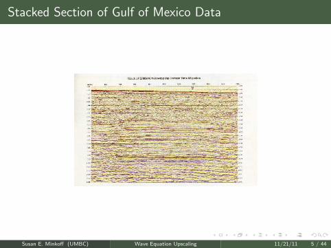
Gulf of Mexico Data from Exxon Production Research Co.

Eleven common-midpoint data gathers.

Radon transform to yield 48 plane-wave traces (per gather) with slowness values from pmin = .1158 ms/m to pmax = .36468 ms/m.

Estimate of anisotropic air gun source in a 31-component Legendreexpansion in slowness, p.

Viscoelastic model (with estimated attenuation coefficient) used asforward simulator for inversion.


Stacked Section of Gulf of Mexico Data


Seismic data in τ − p domain

Figure: The τ − p transformed seismic data from common midpoint gather 6.Data was filtered by convolving it with a 15 Hz Ricker filter.

10 20 30 40

10 20 30 40

0

1000

2000

3000

200

400

600

800

1200

1400

1600

1800

2200

2400

2600

2800

0

1000

2000

3000

200

400

600

800

1200

1400

1600

1800

2200

2400

2600

2800

Plane

Trace

Plane

Trace


Inversion Algorithm:

1 Estimate P-wave background velocity and elastic parameterreflectivities by Differential Semblance Optimization

JDSO [v , r ] =1

2‖S [v , r ] − Sdata‖2 + λ2‖Wr‖2

+σ2‖∂r/∂p‖22 Estimate seismic source and elastic parameter reflectivities (again) by

alternation and Output Least Squares Inversion

JOLS [r , f ] =1

2‖S [r , f ] − Sdata‖2 + λ2‖W [r , f ]‖2


Alternation Algorithm:

Repeat until convergence:

1 Given the current source, fc ,and current reflectivity, rc , invert for anew estimate of the reflectivity r+ using Output Least Squares(i.e., JOLS [r , f ] = 1

2‖dpred [r , f ] − dobs‖2)

2 Replace rc by r+.

3 Given the current source and reflectivity guesses, fc , rc , invert for anew estimate of the source f+ using OLS.

4 Replace fc by f+.


Two Experiments:

1 Model m = three elastic parameter reflectivities. (Source not updatedin inversion)

2 Model m = three elastic parameter reflectivities and seismic source.

In both cases the data is the same. The fixed background velocity is thesame. The starting guesses for the reflectivities are the same (zero). Thealgorithmic stopping tolerances are the same.


Sources

Figure: Left: air gun model source; Right: anisotropic source from inversion


Results:

Inversion-estimated source appears to allow for a better correspondingreflectivity estimate:

Data Fit:1 Experiment 1 (air gun source)

55% rms error.

2 Experiment 2 (inversion-estimated source)

27% rms error.

3 In fact in Experiment 2 (inversion-estimated source)

10% rms error in region around gas sand target.

Model Fit: Experiment 2 reflectivity estimates match well log betterthan Experiment 1 estimates.


Data Misfit Comparison for Two experiments

Figure: Left: 55% data misfit. Right: 29% data misfit

10 20 30 40

10 20 30 40

0

1000

2000

3000

200

400

600

800

1200

1400

1600

1800

2200

2400

2600

2800

0

1000

2000

3000

200

400

600

800

1200

1400

1600

1800

2200

2400

2600

2800

Plane

Trace

Plane

Trace

10 20 30 40

10 20 30 40

0

1000

2000

3000

200

400

600

800

1200

1400

1600

1800

2200

2400

2600

2800

0

1000

2000

3000

200

400

600

800

1200

1400

1600

1800

2200

2400

2600

2800

Plane

Trace

Plane

Trace


Well log comparisons for P-wave impedance

Figure: Left: air gun model source Right: inversion estimated source

1800 1900 2000 2100 2200 2300 2400 2500 2600

−0.25

−0.2

−0.15

−0.1

−0.05

0

0.05

0.1

0.15

0.2

0.25

2−way time (ms)

refle

ctiv

ity (

dim

ensi

onle

ss)

SHORT−SCALE RELATIVE FLUCTUATION IN P−WAVE IMPEDANCE

1800 1900 2000 2100 2200 2300 2400 2500 2600−0.25

−0.2

−0.15

−0.1

−0.05

0

0.05

0.1

0.15

0.2

2−way time (ms)

refle

ctiv

ity (

dim

ensi

onle

ss)

SHORT−SCALE RELATIVE FLUCTUATION IN P−WAVE IMPEDANCE

The solid line shows the inversion result. The dashed line shows thedetrended well log.


For More Detail See...

1 Minkoff, S. E. and Symes, W. W., “Full Waveform Inversion of Marine ReflectionData in the Plane-Wave Domain”, Geophysics, 62 pp. 540–553, 1997.

2 Minkoff, S. E., “A Computationally Feasible Approximate Resolution Matrix forSeismic Inverse Problems”, Geophysical Journal International, 126, pp. 345–359,1996.

3 Minkoff, S. E. and Symes, W. W., “Estimating the Energy Source and Reflectivityby Seismic Inversion”, Inverse Problems 11, pp. 383–395, 1995.


Problem: Running inversion experiments is expensive...


Upscaling

One would like to simulate wave propagation on a coarser scale thanthe one on which the parameters are defined.

We adapted the subgrid upscaling technique developed for ellipticproblems (flow in porous media) to the wave equation.

Goal is to be able to solve the problem on the coarser grid while stillcapturing some of the small scale features internal to coarse gridblocks.

Operator upscaling is one option. Original reference: Arbogast,Minkoff & Keenan, “An Operator-Based Approach to Upscaling thePressure Equation”, Computational Methods in Water Resources XII(1998).

Advantages: No Scale Separation or Periodic Medium Requirements.


Model problem

The Acoustic Wave Equation

1

ρc2

∂2p

∂t2−∇ ·

(1

ρ∇p

)= f

p is the pressurec(x , y) is the sound velocity,ρ(x , y) is the density,f is the source of acoustic energy

The First Order System~v = −1

ρ∇p in Ω,

1

ρc2

∂2p

∂t2= −∇ · ~v + f in Ω,

Boundary conditions~v · ν = 0, on ∂Ω


The finite element method

Find ~v ∈ V and p ∈ W such that〈ρ~v , ~u〉 = 〈p,∇ · ~u〉,⟨

1

ρc2

∂2p

∂t2,w

⟩= −〈∇ · ~v ,w〉 + 〈f ,w〉

for all ~u ∈ V and w ∈ W

W=piecewise discontinuous constant functionsV=piecewise continuous linear functions of the form(a1x + b1, a2y + b2)

Full fine grid

Pressure

Acceleration


Upscaling technique

Goal: Capture the fine scale behavior on the coarser grid

Pressure Unknowns Acceleration Unknowns

Idea: Decompose the solution

~v = ~v c + δ~v

~v c ∈ V c is the coarse-scale solutionδ~v ∈ δV are the fine-grid unknowns internal to each coarse-grid cell –subgrid unknowns


Upscaling technique

Simplifying assumption: δ~v · ν = 0 on the boundary of each coarsecell.

This assumption allows us to decouple the subgrid problems fromcoarse-grid block to coarse-grid block.

We use full fine-grid pressure.


Two steps of upscaling

Step 1: On each coarse element solve the subgrid problem:

Find δ~v ∈ δV and p ∈ W such that〈ρ(~v c + δ~v), δ~u〉 = 〈p,∇ · δ~u〉,⟨

1

ρc2

∂2p

∂t2,w

⟩= −〈∇ · (~v c + δ~v),w〉 + 〈f ,w〉

for all δ~u ∈ δV and w ∈ WNote: the value of ~v c is unknown at this stage.The subgrid problem fully determines p.

Step 2: Use the solution of subgrid problem to solve the coarseproblem:

Find ~v c ∈ V c such that

〈ρ(~v c + δ~v), ~uc〉 = 〈p,∇ · ~uc〉, for all ~uc ∈ V c


Parallel implementation

Serial cost

(Np + 2Nu)Nδ Nc + O(Nc)

Parallel cost

(Np + 2Nu)Nδ Nc

p+ O(Nc)

Np and Nu are the number of flops required to solvefor pressure and acceleration respectively,Nδ and Nc are the sizes of the subgrid and coarse problems,p is the number of processors.

Subgrid problems: Embarrassingly parallel.

No communication between processors.No ghost-cell memory allocation required.

Coarse problem: Solve in serial.

Post-processing: Cheap and fast.


Timing Studies

Numerical grid contains 3600 × 3600 fine grid blocks and 36 × 36 coarse gridblocks.timings are for 20 time steps.

number total subgrid coarse post-of processors time problems problem processing

1 29.70 29.69 0.00060 0.00262 15.46 15.38 0.00045 0.07114 7.63 7.56 0.00049 0.07076 5.23 5.14 0.00048 0.07498 4.37 4.26 0.00046 0.089612 3.07 2.94 0.00045 0.1150

References: Vdovina, T., Minkoff, S., and Korostyshevskaya, O., “Operator Upscaling forthe Acoustic Wave Equation”, Multiscale Modeling and Simulation, 4, pp. 1305–1338,2005.

Vdovina, T. and Minkoff, S., “An A Priori Error Analysis of Operator Upscaling for the

Acoustic Wave Equation”, International Journal of Numerical Analysis and Modeling, 5,

pp. 543–569, 2008.


Timing Studies:

number of Finite-difference Upscaling codeprocessors code number of fine blocks per coarse block

100 × 100 100 × 100 60 × 60 50 × 50 40 × 40

1 29.43 29.69 29.92 30.31 31.012 – 15.46 15.35 15.61 16.134 – 7.63 7.97 8.59 8.846 – 5.23 5.62 5.88 6.378 – 4.37 5.12 7.52 7.2012 – 3.07 3.82 3.97 4.43

Note: Performance improves as coarse block size increases.


Numerical Experiment I (Acoustic Wave Equation)

Domain is of size 10 × 10 km.

Fine grid: 1000 × 1000. Coarse grid: 100 × 100.

Gaussian source, 200 time steps.

Sound velocity strips range from 3500 m/s to 7500 m/s.


Vertical Acceleration

Full finite-difference soln Reconstructed Upscaled Soln


Numerical Experiment II (Elastic Wave Equation)

Fine grid: 320 × 320 × 320. Coarse grid: 80 × 80 × 80.

Source is Gaussian in space, Ricker in time.

Wave propagates about 7 wavelengths.

Mixture of two materials with Vp = 2.5 km/s or 3 km/s; Vs = 1.5 and 1.75 km/srespectively, ρ = 2.2 · 1012 and 2.3 · 1012 kg/km3.


yz slices of first component of velocity solution

z

y

0 4 8 12 16 20 24 28 32

0

4

8

12

16

20

24

28

32 −8

−6

−4

−2

0

2

4

6

8

10

12x 10

−10

z

y

0 4 8 12 16 20 24 28 32

0

4

8

12

16

20

24

28

32

−8

−6

−4

−2

0

2

4

6

8

10

12

x 10−10

Full finite-element soln Augmented Upscaled Soln

Reference: Vdovina, T., Minkoff, S., and Griffith, S., “A Two–Scale Solution Algorithm

for the Elastic Wave Equation,” SIAM Journal on Scientific Computing, 31, pp.

3356-3386, 2009.


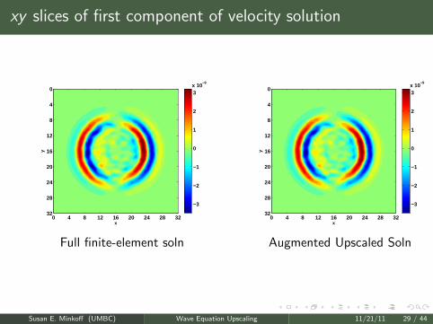
xy slices of first component of velocity solution

y

x

0 4 8 12 16 20 24 28 32

0

4

8

12

16

20

24

28

32

−3

−2

−1

0

1

2

3x 10

−9

y

x

0 4 8 12 16 20 24 28 32

0

4

8

12

16

20

24

28

32

−3

−2

−1

0

1

2

3x 10

−9

Full finite-element soln Augmented Upscaled Soln


Comparison of time traces for the first component ofvelocity

Red curve = full finite element solution. Green curve = coarse solution.Blue curve = full finite element solution for the homogeneous mediumwith a single (average) value for each of the three input parameter.

0 1 2 3time (s)

-6

-4

-2

0

2

x10 -10

fisrt

com

pone

nt o

f vel

ocity

(km

/s)

0 1 2 3time (s)

0

1

2

x10 -9

fisrt

com

pone

nt o

f vel

ocity

(km

/s)

Receiver at (16 km, 8 km, 12 km) Receiver at (16 km, 8 km, 18 km)


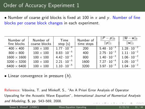
Order of Accuracy Experiment 1

• Number of coarse grid blocks is fixed at 100 in x and y . Number of fineblocks per coarse block changes in each experiment.

Number of Number of Time Number of||P − p||0||p||1

||U − u||0||u||1fine blocks coarse blocks step (s) time steps

400 × 400 100 × 100 1.77 · 10−4 200 5.48 · 10−3 1.28 · 10−2

800 × 800 100 × 100 8.83 · 10−5 400 2.75 · 10−3 1.11 · 10−2

1600 × 1600 100 × 100 4.42 · 10−5 800 1.40 · 10−3 1.06 · 10−2

3200 × 3200 100 × 100 2.21 · 10−5 1600 7.27 · 10−4 1.05 · 10−2

6400 × 6400 100 × 100 1.10 · 10−5 3200 3.97 · 10−4 1.04 · 10−2

• Linear convergence in pressure (h).

Reference: Vdovina, T. and Minkoff, S., “An A Priori Error Analysis of Operator

Upscaling for the Acoustic Wave Equation”, International Journal of Numerical Analysis

and Modeling, 5, pp. 543–569, 2008.


Order of Accuracy Experiment 2

• Number of fine grid blocks is fixed at 6400 in x and y . Number ofcoarse blocks varies in each experiment.

Number of fine blocks Number of coarse blocks||P − p||0||p||1

||U − u||0||u||1

6400 × 6400 100 × 100 3.97 · 10−4 1.04 · 10−2

6400 × 6400 200 × 200 3.50 · 10−4 5.24 · 10−3

6400 × 6400 400 × 400 3.41 · 10−4 2.65 · 10−3

6400 × 6400 800 × 800 3.39 · 10−4 1.38 · 10−3

6400 × 6400 1600 × 1600 3.39 · 10−4 7.97 · 10−4

• Linear convergence in acceleration (H).


An Alternate Analysis:

Reference: Korostyshevskaya, O. and Minkoff, S., “A Matrix Analysis of Operator-Based

Upscaling for the Wave Equation”, SIAM J. Numer. Anal., 44, pp. 586–612, 2006.

Recall two steps of upscaling algorithm:

Subgrid problems: On each coarse element solve the subgrid problem:

Find δ~v ∈ δV and p ∈ W such that〈ρ(~v c + δ~v), δ~u〉 = 〈p,∇ · δ~u〉,⟨

1

ρc2

∂2p

∂t2,w

⟩= −〈∇ · (~v c + δ~v),w〉 + 〈f ,w〉

for all δ~u ∈ δV and w ∈ W

Coarse problem: Use the solution of subgrid problem to solve the coarseproblem:

Find ~v c ∈ V c such that

〈ρ(~v c + δ~v), ~uc〉 = 〈p,∇ · ~uc〉, for all ~uc ∈ V c

Use finite element expansions to obtain the matrix-vector form

Subgrid problems:Acf vc

x + Aff δvx = B f p

W∂2p

∂t2= −(Bc)Tvc

x − (B f )T δvx − (vy terms) + F

Coarse problem:Accvc

x + (Acf )T δvx = Bcp

Matrix entries

affl ,n = 〈ρ(δux)n, (δux)l〉 acf

l ,i = 〈ρ(ucx )i , (δux)l〉 acc

l ,i = 〈ρ(ucx )i , (u

cx )l〉

wl ,m =

⟨1

ρc2wm,wl

⟩bfl ,m =

⟨wm,

∂(δux)l∂x

⟩bcl ,m =

⟨wm,

∂(ucx )l

∂x

⟩fl = 〈f ,wl〉


Matrix equation

Idea: Eliminate the subgrid acceleration from the coarse equation

Subgrid problem

δvx = −(Aff )−1Acf vcx + (Aff )−1B f p

Coarse problem

(Acc − (Acf )T (Aff )−1Acf )vcx = (Bc − (Acf )T (Aff )−1B f )p

Obtain a matrix equation for the coarse acceleration and pressure only

Uvcx = Dp

Find explicit formulas for the entries of U and D to derive a differenceequation


Differential equation

Differential equation (from Taylor series expansion)

ρupsv cx = −∂p

∂x

ρups is the upscaled density given by the average of the density values onthe boundary of the coarse cell.

PP rl

Recall one of two original continuous pde’s in our system: ~v = −1

ρ∇p


Pressure Equation Analysis

Assuming appropriate smoothness on pressure p and density ρ, theupscaling algorithm solves the following differential equation for pressureinside a coarse block:

1

ρc2

∂2p

∂t2=

∂

∂x(ρ−1∂p

∂x) +

∂

∂y(ρ−1 ∂p

∂y) + f ,

[order of approximation O(h2x + h2

y )].

Along coarse block edges upscaling satisfies the following equation forpressure:

1

ρc2

∂2p

∂t2=

∂

∂x

((ρups)−1∂p

∂x

)+

((ρups)−1 ∂2p

∂x∂y

)K+

∂

∂y

((ρups)−1 ∂p

∂y

)+f ,

[order of approximation O(hx + hy )] and K is a constant which dependson the location of the pressure node within a single coarse cell.


Solving the Inverse Problem

Want to find c given some observed p.

Easier to find m = 1c2 , squared slowness.

The least squares functional is given by

J (m) =1

2

∑s,r

[∫ T

0(Ss,rp − ds,r )

2 + (Ts,r (∇p) − bs,r )2 dt

].

s and r are indices over source and receiver position.

bs,r and ds,r are observed values for p and ∇p.

Ss,r and Ts,r are sampling operators, restricting the values of p and∇p to locations with observed values.

(Reference: Plessix, A Review of the Adjoint State Method For Computing the Gradientof a Functional with Geophysical Applications)


The Formal Optimization Problem

Find minm J (φ,m) s.t. F (φ,m) = 0.

φ is the state variable (pressure).

m is the control variable (squared slowness).

F (φ,m) = 0 is the forward problem (the wave equation).

Method: δmJ = δφJ δmφ+ δemJ .

δemJ is the explicit variation of J w.r.t. m.

Problem: How do we find δmφ?

(Reference: Gunzburger’s Perspectives in Flow Control and Optimization.)


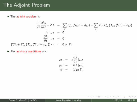
The Adjoint Problem

The adjoint problem is:

1

c2

∂2λ

∂t2− ∆λ =

∑r

S∗s,r (Ss,rp − ds,r ) −∑

r

∇ · T ∗s,r (Ts,r (∇p) − bs,r )

λ |t=T = 0

∂λ

∂t|t=T = 0(

∇λ+ T ∗s,r (Ts,r (∇p) − bs,r )

)· ν = 0 on Γ.

The auxiliary conditions are:

µ0 = m∂λ

∂t|t=0

µ1 = −mλ |t=0

ψ = −λ on Γ.


Obtaining an Expression for the Gradient

Question: How do we get DmJ (n) (x , y)?

To get DmJ (n) (x , y) from δmJ , we let m be δ (x , y).

This gives:

(DmJ ) (x , y) = −∑

s

[∫ T

0

∂2p (x , y)

∂t2λ (x , y) dt

].

To calculate the gradient, we must have access to both the forwardand adjoint solutions at all time steps.

Use a checkpointing scheme to optimally determine what to store andwhat to recalculate.

(Reference: Gunzburger’s Perspectives in Flow Control and Optimization.)


An Optimization Algorithm

Beginning with m(0) (x , y), we repeat the following:

1 Solve the forward problem to get the state variables p(n) (x , y , t) andthen solve the adjoint problem to get the adjoint variable λ(n) (x , y , t).

2 Calculate the gradient DmJ (n) (x , y) = −∑

s

[∫ T

0∂2p(x,y)

∂t2 λ (x , y) dt].

3 Update squared slowness for the next step:

m(n+1) (x , y) = m(n) (x , y) + βn

∑s

[∫ T

0

∂2p (x , y)

∂t2λ (x , y) dt

],

using some step size βn.


The Upscaled Adjoint Problem

Introduce χ = −∇λ and decompose χ into δχ+ χc .

Then, for each subgrid problem,

(χc + δχ, δu) = (λ,∇ · δu)(1

c2

∂2λ

∂t2,w

)= − (∇ · (χc + δχ) ,w)

+

(∑r

S∗s,r (Ss,rp − ds,r ) −∑

r

∇ · T ∗s,r (Ts,r (∇p) − bs,r ) ,w

)

for w ∈ W and δu ∈ δV .

And, for each coarse problem,

(χc + δχ,uc) = (λ,∇ · uc)

for uc ∈ V c .


Conclusions

To speed up an expensive iterative process like seismic inversion, operator upscalingcan be applied to the wave equation.

The upscaled solution captures some of the sub-wavelength heterogeneities of thefull solution.

For the acoustic implementation, the method exhibits good parallel performancedue to the independence of the subgrid problems (most expensive part of thealgorithm).

A matrix analysis of the algorithm indicates that, in fact, the upscaling technique issolving the continuous differential equation with density given by averaging alongcoarse block edges.

The pressure equation corresponds to the standard acoustic wave equation at nodesinternal to coarse blocks.

Along coarse cell boundaries, the upscaled solution solves a modified wave equationwhich includes a mixed second-derivative term.

Using the adjoint method we can reuse much of the upscaling code to solve theinverse problem.


Acknowledgments

This research was performed with funding from the CollaborativeMath-Geoscience Program at NSF (grant #EAR–0222181), theComputational Mathematics Program at NSF (grant #DMS–0714159), aGAANN grant from the U.S. Department of Education (Award#P200A030097), a generous fellowship provided by NASA Goddard’sEarth Sciences and Technology Center (GEST), and UMBC’s ADVANCEgrant (NSF #SBE-0244880).


Date post:	30-Dec-2019
Category:	Documents
Upload:	others
View:	2 times
Download:	0 times

Two-Scale Wave Equation Modeling for Seismic Inversion · Two-Scale Wave Equation Modeling for...

Documents