1 / 29

Two-Stage Convolutional Neural Network Architecture for

Lung Nodule Detection

Haichao Cao, Hong Liu*, Enmin Song, Guangzhi Ma, Xiangyang Xu,

Renchao Jin, Tengying Liu, Chih-Cheng Hung

Abstract

Early detection of lung cancer is an effective way to improve the survival rate of

patients. It is a critical step to have accurate detection of lung nodules in computed

tomography (CT) images for the diagnosis of lung cancer. However, due to the

heterogeneity of the lung nodules and the complexity of the surrounding environment,

robust nodule detection has been a challenging task. In this study, we propose a

two-stage convolutional neural network (TSCNN) architecture for lung nodule

detection. The CNN architecture in the first stage is based on the improved UNet

segmentation network to establish an initial detection of lung nodules. Simultaneously,

in order to obtain a high recall rate without introducing excessive false positive

nodules, we propose a novel sampling strategy, and use the offline hard mining idea

for training and prediction according to the proposed cascaded prediction method. The

CNN architecture in the second stage is based on the proposed dual pooling structure,

which is built into three 3D CNN classification networks for false positive reduction.

Since the network training requires a significant amount of training data, we adopt a

data augmentation method based on random mask. Furthermore, we have improved

the generalization ability of the false positive reduction model by means of ensemble

learning. The proposed method has been experimentally verified on the LUNA dataset.

Experimental results show that the proposed TSCNN architecture can obtain

competitive detection performance.

Keywords: lung nodule detection; UNet; 3D CNN; ensemble learning;

computer-aided diagnosis

1 Introduction

Lung cancer is one of the most dangerous diseases leading to cancer death,

2 / 29

accounting for two-thirds of all cancers [1, 2]. Its 5-year survival rate is 18% [3].

Clinical experience has shown that if lung cancer can be diagnosed at an early stage,

the chance of survival will be greatly increased [4]. The use of diagnostic methods

based on computed tomography (CT) images is an important strategy for early

diagnosis of lung cancer and improvement of patient survival [5]. Accurate detection

of lung nodules is an important step in the diagnosis of early stage lung cancer in

medical imaging-based diagnostic methods. With an increasing number of CT images

of lung nodules, in order to reduce the cumbersome manual labeling and the

variability of detection results, it is of great clinical significance to develop robust

automatic detection models [6] .

In recent years, although many methods of lung nodule detection has been

proposed [7-9] , it is still difficult to obtain satisfactory detection result due to the

heterogeneity of lung nodules on CT images (as shown in Fig. 1). For example, for

calcific nodules (Fig. 1 (tp2)), cavitary nodules (Fig. 1 (tp3)) and ground-glass opacity

nodules (Fig. 1 (tp4)), they reflect the heterogeneity of lung nodules in terms of shape,

texture and intensity. In addition, the development of a robust detection model is also

a challenge due to the high degree of similarity between the lung nodules and their

surrounding tissues. For example, for juxtapleural nodules (Fig. 1 (tp5)), since the

lung nodules are almost identical, in terms of intensity, to the lung wall, it is difficult

to automatically locate its exact location. Similarly, for small lung nodules less than 6

mm in diameter such as Fig. 1 (tp6) (corresponding to the green rectangle box) are

difficult to distinguish because they have similar intensities to the surrounding noise

which can be seen in Fig. 1 (fp6) (corresponding to the red rectangle box).

Furthermore, to illustrate the similarity between lung nodules and non-lung nodules,

we list six false positive lung nodules in the second row of Fig. 1 (Fig. 1 (fp1-6)).

(tp₁) isolated nodule (tp₅) juxtapleural nodule(tp₃) cavitary nodule(tp₂) calcific nodule (tp₄) GGO nodule (tp₆) small nodule

(fp₁) (fp₅)(fp₃)(fp₂) (fp₄) (fp₆)

Fig. 1. Example images of lung nodules with different locations and shapes in CT image. Note that

the GGO in sub-figure (tp4) represents a ground-glass opacity nodule, and sub-figure (tp6) is a

small nodule with a diameter of 4.4 mm. Among them, the sub-figure (fp1-6) represents the false

positive nodule having similar appearance characteristics to the true lung nodule.

To solve the problems discussed above in the heterogeneous CT data, we propose

3 / 29

a two-stage convolutional neural network (TSCNN) in this study. This network

architecture is divided into two stages: the candidate nodule detection stage which is

based on the improved UNet and the false positive reduction stage which is based on

3D CNN. The purpose of the first stage is to obtain a region of interest where a lung

nodule may be present; the purpose of the second stage is to reduce false positives in

candidate nodules obtained by the first stage. In general, TSCNN can detect various

types of lung nodules to achieve a better detection rate. Our technical contributions in

this work are the followings.

(1) A UNet segmentation network based on ResDense structure (Section 3.1.1)

was designed and used to perform initial detection of lung nodules. In addition, we

propose a new sampling strategy (Section 3.1.2) to select samples for training, and

then train based on the offline hard mining idea (Section 3.1.3) to make the model

suitable for those indistinguishable samples. Finally, using the proposed cascade

prediction method (Section 3.1.5) for prediction can effectively reduce false positive

nodules.

(2) Based on the design of the dual pooling approach, we have built three 3D

CNN network architectures dedicated to reducing false positive lung nodules, which

are based on SeResNet (Section 3.2.1), DenseNet (Section 3.2.2) and InceptionNet

(Section 3.2.3) classification networks. It is worth noting that in order to obtain a

better classification effect; we propose a data augmentation method based on random

mask (Section 3.2.4). In addition, we have further improved the generalization ability

of the proposed false positive reduction model by means of ensemble learning.

2 Related works

The detection of lung nodules usually involves two stages: one is the detection of

candidate lung nodules and the other is the reduction of false positive lung nodules. In

recent years, many solutions have been proposed. These methods can be generally

divided into traditional detection methods, machine learning algorithms, and methods

based on convolutional neural networks. Please note that the lung nodules will be

referred to the nodules.

In the traditional detection method, in order to detect nodules from the very

complex lung environment, morphological operations, threshold-based methods,

clustering algorithms and energy optimization algorithms have been widely used

[10-16]. For example, Gupta et al. developed a lung mask by combining masks,

flooding fill algorithms, and morphological operations, and then performed nodule

detection based on a multi-level thresholding algorithm combined with various feature

4 / 29

extraction techniques [17]. Rezaie et al. first selected a region of interest that may

have nodules based on the threshold method, and then used an edge detection

algorithm to locate the nodule [18]. Typically, Lu et al. propose a hybrid algorithm for

nodule detection that integrates traditional methods such as morphological operations,

Hessian matrices, fuzzy sets, and regression trees [19].

In machine learning methods, researchers combine the classification models with

advanced features for the detection of nodules [20-25]. For example, Froz et al. used

artificial crawler and rose diagram techniques to extract texture features of nodules

and then use radial basis kernel based support vector machines (SVM) for

classification [26]. Similarly, Aghabalaei et al. designed a set of spectral, texture, and

shape features to characterize nodules, and then used the SVM to classify candidate

nodules [27]. Nithila et al. developed a Computer-Aided Detection (CAD) system for

isolated lung nodule detection that focuses on heuristic search algorithms and uses

particle clustering algorithms for network optimization [28]. In addition, Alam et al.

proposed a patch-based multi-spectral method for nodules detection [29].

In the methods based on convolutional neural network (CNN), the researchers

train the nodule detection model end-to-end in a supervised learning manner, while

using the CNN to learn the relevant features of the nodule to replace traditional

feature extraction methods. Within the CNN methods, the 2D CNN method has been

widely used [30-38]. For example, Ciompi et al. used a combination of three views of

the axial, sagittal, and coronal planes as input to the nodule detection model and used

ensemble learning for prediction [39]. One year later, Setio et al. integrated the six

diagonal views of the nodule into the input of the nodule detection model, each of

which was processed by a ConvNets stream. The confidence of the candidate nodule

is obtained by fusing the output of nine ConvNets which have the same structure [40].

George et al. used a YOLO-based method which is a method for object detection in

natural images to detect lung nodules in CT images [41]. Meanwhile, some other

researchers use 3D deep CNNs for the detection of nodules [42-46]. For example,

Hamidian et al. use a fully convolutional network to generate negative samples that

are difficult to be identified correctly, and then train a 3D CNN for nodule detection

based on these negative samples [47, 48]. In order to simplify the detection process of

nodules, Jenuwine et al. developed a CAD system that uses 3D CNN to detect nodules

in CT images without using false positive reductions in candidate nodules, but the

detection accuracy is far from expected [49]. Typically, a new 3D CNN with dense

connections proposed by Khosrava et al., which is trained in an end-to-end manner,

does not require any post-processing or user guidance to improve the detection results

[50].

The TSCNN architecture proposed in this paper differs from the previous

5 / 29

methods in the following aspects: 1) using the improved UNet segmentation model

for lung nodule detection; 2) for the segmentation model training, we propose a new

sampling strategy and an offline hard mining training approach; 3) we propose a

cascade prediction method different from the traditional prediction method; 4) build

three 3D CNN classification networks based on the dual pooling method; 5) design a

data augmentation method based on random mask.

3. Methods

The lung nodule detection framework proposed in this paper is divided into two

stages. The first stage: the detection of candidate nodules, which is based on the UNet

architecture to achieve the detection of candidate nodules by segmenting suspicious

nodules. The second stage: the reduction of false positive nodules, which is based on

the 3DCNN architecture to eliminate false positive nodules through the integration of

multiple models. The overall architecture of the proposed lung nodule detection

method is shown in Fig. 2.

Candidate nodule detection False positive reduction

Design network

architecture

Training network

model

Design network

architecture

Training network

model

Fig. 2. The flowchart of the proposed two-stage CNN. Two stages are shown inside the blue and

green boxes, respectively.

Section 3.1 describes the detection methods for candidate nodules, and Section

3.2 gives the false positive reduction methods for candidate nodules.

3.1. Candidate nodule detection

In this study, we use the UNet-based segmentation network to detect candidate

nodules. In order to better detect candidate nodules, we improved the original UNet

architecture and proposed a novel sampling strategy. In addition, to further reduce

6 / 29

false positive nodules, we use the idea of the offline hard mining to train and use

cascaded prediction methods for prediction.

3.1.1. Network architecture

Fig. 3 shows the proposed UNet segmentation architecture based on the

residual-dense mechanism for initial lung nodule detection. The architecture consists

of six residual dense blocks (ResDenseBlock1, ResDenseBlock2,..., ResDenseBlock6

in Fig. 3(a)), three 2D max pooling layers (three blue arrows in Fig. 3(a)), and three

2D deconvolution layers (three yellow arrows in Fig. 3(a)), and one sigmoid

regression layer. Six residual dense blocks can be divided into two groups (each group

contains three residual dense blocks), one for feature extraction including

ResDenseBlock1, ResDenseBlock2, ResDenseBlock3, and the other for feature

reconstruction including ResDenseBlock4, ResDenseBlock5, ResDenseBlock6. Each

of the residual dense blocks described above is composed of the stack of six dense

blocks, and one residual connection. Fig. 3(b) shows the basic unit-dense block

constituting the residual dense block. The three 2D max pooling layers are separately

used after three residual dense blocks in feature extraction. The three 2D

deconvolution layers are used after three residual dense blocks in feature

reconstruction. It should be noted here that the input of each residual dense block in

feature reconstruction is the concatenation of the output of the upper layer and the

output of its corresponding feature extraction layer.

In the specific experiment, the pooling kernel size, the stride and padding method

of the three max pooling layers in Fig. 3(a) are 3×3, 2 and “same”, respectively. The

convolution kernel size, the stride and the padding method of the three deconvolution

layers are the same as the max pooling layer. In addition, the number (i.e., n) of

feature maps corresponding to different residual dense blocks in Fig. 3(b) is varied.

The value of n corresponding to ResDenseBlock1 and ResDenseBlock6 is 8, the value

of n corresponding to ResDenseBlock2 and ResDenseBlock5 is 16, and the value of n

corresponding to ResDenseBlock3 and ResDenseBlock4 is 32.

7 / 29

3x3, n 3x3, n ConcateDropout, BN, ReLUBN, ReLU

DenseBlock(b)

DenseBlock6 Concate

ResDenseBlock(c)

DenseBlock2DenseBlock1

Con

cate

Con

cate

Co

nca

te

ResDenseBlock1

ResDenseBlock2

ResDenseBlock3 ResDenseBlock4

ResDenseBlock5

ResDenseBlock6

Sigmoid

(a)

: Deconv : MP

Fig. 3. (a) The proposed UNet segmentation architecture based on the residual-dense mechanism,

(b) the diagram of the Dense block (DenseBlock), and (c) the diagram of the residual dense block

(ResDenseBlock). The parameter "n" indicates the number of feature maps.

3.1.2. Sampling strategy

For the segmentation of lung nodules, the edge voxels of the nodules are crucial

because they usually contain more texture information. If the edge voxels of the lung

nodules are well recognized, a complete nodule mask can be obtained by simple

morphological operation even if the internal segmentation of the nodules is

incomplete. Based on this idea, when sampling the voxels of the lung nodule class, we

consciously pay attention to the voxels on the edge of the lung nodules. Specifically,

the corresponding sampling weight (the probability that a voxel is sampled) is set

according to the minimum distance between each voxel and the lung nodule edge

voxel. The smaller the distance is, the larger the weight will be. In addition, in order to

have samples near the voxel which is close to the center of the nodule, we use the

radius of the lung nodule as an adjustment factor to suppress the polarization of the

sampling weight.

The calculation formula for the sampling weight of the voxel in the lung nodule

class is shown in (1).

8 / 29

min ( , )

r

min ( , )

r

exp,

exp

t E

t E

d k t

k d k tPW k P

(1)

where PWk represents the sampling weight of the k-th voxel in the lung nodule class;

P the lung nodule class; E the set of voxels belonging to the edge of the lung nodule;

d(k, t) the Euclidean distance between the k-th voxel in P and the t-th voxel in E, and r

the radius of the lung nodule.

For the sampling of voxels in non-lung nodule class (such as blood vessels, lung

walls, lung parenchyma, etc.), we divide them into two categories based on the

distance from the currently sampled lung nodules. One class is the set of voxels that

are closer to the currently sampled lung nodules (high correlation background class),

and the corresponding sampling region is a local region (green region in Fig. 4) other

than the lung nodules. The other class is the set of voxels that are farther from the

currently sampled lung nodules (low correlation background class), and the

corresponding sampling region is the region outside the high correlation background

class sampling region (gray region of Fig. 4).

L

LL

L

Fig. 4. The schematic diagram of the corresponding local region when sampling various voxels.

The entire gray rectangle box represents one of the slices of the currently sampled nodule, and the

red-labeled round (lung nodule) is a sampling region of the lung nodule; the blue dotted

rectangular box representing the circumscribed rectangle of the lung nodule. In addition, the green

rectangular region outside the lung nodule represents the sampling region of the high correlation

background class, and the size of the green rectangular box is determined by the size of the lung

nodule and the "L" value, where "L" indicates the length (the value in the experiment is 64) of the

9 / 29

image patch used to train the UNet segmentation model. The gray region outside the green

rectangle box indicates the sampling region of the low correlation background class.

In general, for the sampling of the voxels of non-lung nodule class, we consider

their corresponding intensity information when calculating their sampling weights.

This is because, compared with the lung parenchyma, air, and other low-intensity

voxels, the lung wall, blood vessels, and the like with higher intensity are more

similar to the lung nodules. Especially the juxtapleural nodules (the intensity of the

adhered lung wall is almost the same as the intensity of the lung nodules). Therefore,

for these indistinguishable voxels, a larger weight should be given, and the

corresponding weight calculation formula is as shown in (2).

min ( , )

r

min ( , )

r

exp,

exp

j E

j E

d i j

ii d i j

i

IHBW i HB

I

(2)

where HBWi represents the sampling weight of the i-th voxel in the high correlation

background class; HB the high correlation background class; d(i, j) the Euclidean

distance between the i-th voxel in HB and the j-th voxel in E, and Ii the intensity value

of the i-th voxel in HB.

For the voxels in low correlation background class that are far from the lung

nodules, we consider the distance information between the voxels and the nodules in

addition to the intensity information. The difference from the above is that the greater

the distance from the center of the lung nodule (in order to speed up the sampling

speed, where the distance from the edge of the lung nodule is not used) is, the greater

the sampling weight will be. This is because the samples used to train the model

should not all be voxels near the lung nodules, and some low correlation voxels

should be sampled for training to improve the robustness of the model, thereby

reducing false positive lung nodules. It should be noted that if the voxels sampled at

this time belong to the lung nodule class, they should be eliminated. The calculation

formula for the sampling weight of the low correlation background class is shown in

(3).

( , ),

( , )

p

p

p

I d p cLBW p LB

I d p c

(3)

where LBWp represents the sampling weight of the p-th voxel in the low correlation

background class; LB the low correlation background class; c the central voxel of the

currently sampled lung nodule; d(p,c) the Euclidean distance between the p-th voxel

in LB and the voxel c, and Ip the intensity value of the p-th voxel in LB .

Finally, we also need to determine the number of voxels that are sampled for

10 / 29

each lung nodule. In order to adequately sample nodules of various sizes without

introducing too many redundant samples, we only refer to the number of voxels on

the edge of the nodule, not all voxels corresponding to the nodule. In the specific

experiment, we set the total number of sampling points to 2.5 times the number of

lung nodule edge voxels (N). In order to roughly balance various class of training

samples, the number of sampling points of lung nodule class, high correlation

background class and low correlation background class are N, N and 0.5N,

respectively.

All of the above three sampling methods are to sample the slice containing the

lung nodules. We know that the largest diameter of the lung nodules is 30mm (the

lung nodules can span up to 30 slices), only a small part of the total number of slices

(average of 300 slices), that is, many slices that do not contain lung nodules are not

sampled which greatly reduces the generalization ability of the model. In the actual

sampling process, if the slice containing no lung nodules is sampled according to the

sampling rule of non-lung nodule class described above, or a simpler random

sampling strategy is used, many redundant samples are inevitably introduced.

Moreover, the scale of the training set will be expanded significantly, which will make

the model difficult to converge, and will also greatly extend the training time of the

model. To solve this problem, we do not directly sample the slice that does not contain

the pulmonary nodules, but based on the idea of the offline hard mining, using the

initial model M to predict the slice that does not contain the lung nodules, and then

the samples of prediction error are treated as the sample sampled on the slice that

does not contain a lung nodule, and finally added to the training set to continue

training. The model M is the model obtained by training the sample sampled only

from the slice containing the lung nodule.

3.1.3. Offline hard mining

As described in Section 3.1.2, in order to improve the robustness of the model

and further reduce false positives, we indirectly sample the slices that do not contain

lung nodules using the hard mining method. Specifically, we use the initial model M

to predict the CT data in the training set. If any mask is segmented in the slice that

does not contain the lung nodule, they will all be considered as difficult negative

samples, and then their central voxels will be taken as our sampling points in the

non-lung nodule slice. It should be noted that when predicting the slice containing the

nodule (the segmentation mask does not intersect with the gold standard); the

predicted result may also contain false positive lung nodules, which also need to be

sampled. In addition, we still need to sample the lung nodule voxels to ensure the

11 / 29

balance between the positive sample (the training sample containing some or all of the

nodule mask in the label) and negative sample (the training sample that do not contain

any nodule masks in the label) in retraining. However, for sampling, we are not

randomly selecting voxels from the previously sampled lung nodules class that are

equivalent to the number of negative samples. Instead, the number of samples of

voxel of lung nodule class is dynamically adjusted based on the overlap rate between

the current nodule and the gold standard. It is assumed that the number of edge points

of the current nodule is C, and the overlap rate [51] with the gold standard is O, then

the number of voxels sampled for this nodule is T=C*(1-O). The meaning of this

formula is that the better the segmentation of the current nodule is, the fewer the

number of corresponding sampling points will be. On the contrary, it indicates that the

segmentation result of the model on the current nodule is not good, so it is necessary

to pay attention to it, and the number of corresponding sampling points should also be

increased.

3.1.4. Training procedure

In the actual training process, we crop the 64*64*3 size data patch centered on

the voxels sampled from the slice containing the nodules for training the initial

segmentation model M. When the training is completed, the model M is used to select

difficult positive and negative samples, and then fine-tuned based on the initial model

M to improve the generalization ability of the model. It should be noted that in the

experiment, we use the Adam optimizer [52] to update the model parameters. In order

to prevent over-fitting, we adopted a training strategy for early stop [53]. Specifically,

if the performance of the model is not improved, the training continues for 5 epochs,

and the total training algebra is 15 epochs. In addition, our initial learning rate is

0.0001, the learning rate when fine-tuning is 0.00001, and the batch size is 64.

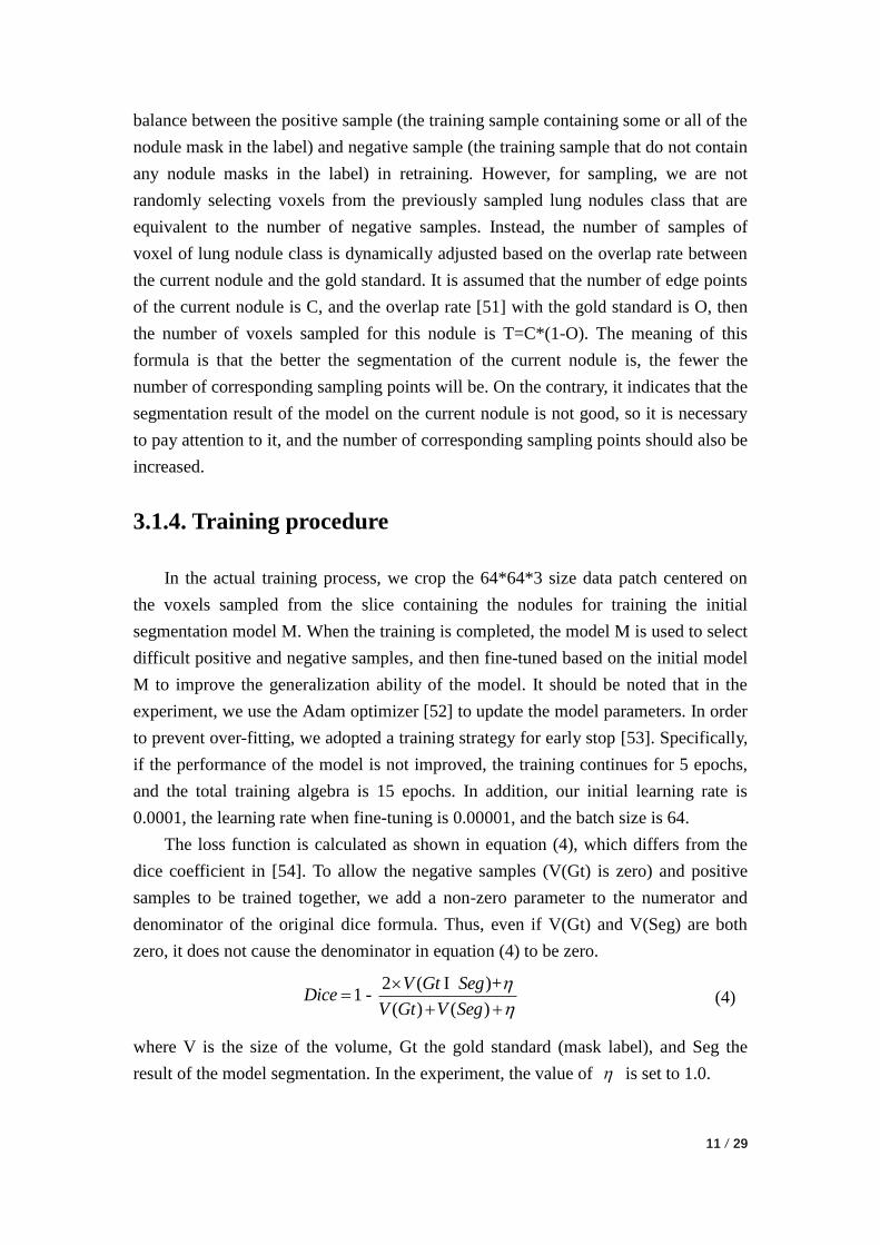
The loss function is calculated as shown in equation (4), which differs from the

dice coefficient in [54]. To allow the negative samples (V(Gt) is zero) and positive

samples to be trained together, we add a non-zero parameter to the numerator and

denominator of the original dice formula. Thus, even if V(Gt) and V(Seg) are both

zero, it does not cause the denominator in equation (4) to be zero.

2 ( )+1 -

( ) ( )

V Gt SegDice

V Gt V Seg

I (4)

where V is the size of the volume, Gt the gold standard (mask label), and Seg the

result of the model segmentation. In the experiment, the value of is set to 1.0.

12 / 29

3.1.5. Cascaded prediction

When the model training is completed, we predict the entire CT image by sliding

the data patch of size 128*128*3 (stride size 64). For overlapping regions, in order to

ensure a high recall rate, we use the union of the predicted results as the final

segmentation result, but this will introduce more false positives nodules. To alleviate

this problem, we take the result of this sliding prediction as the center, extract

64*64*3 data blocks, and send them into the model for secondary prediction. The

purpose of this is to make an accurate segmentation in the local region where the

suspected nodule is located. Because even if the suspected nodule is not a true lung

nodule, narrowing the prediction area to the size of the data patch used during training

will be more conducive to model prediction.

Table 1. Results of the cascading predictions on the testing set. Among them, The FPS indicates

false positive rate and SEN shows sensitivity.

FPS Sen

First Prediction 139.40 0.988

Second Prediction 37.83 0.954

First Prediction Second Prediction

First Prediction Second Prediction

Second Prediction

Second Prediction

First Prediction

First Prediction

Fig. 5. Segmentation results for the first stage segmentation model in layers that do not contain

lung nodules (first row) and layers that contain lung nodules (second row). The first and second

prediction results are drawn in the second column and the fourth column, where red indicates the

rectangular box corresponding to the model segmentation result, and green specifies the

rectangular box corresponding to the gold standard.

To verify the effect of the cascade prediction, we only evaluate the results of the

first stage using the segmentation model for nodule detection. The evaluation results

are shown in Table 1. As can be seen from Table 1, the false positive rate has dropped

nearly fourfold when the recall rate has only decreased by less than four percentage

13 / 29

points. In addition, in order to more intuitively observe the necessity of the second

prediction, we randomly selected the segmentation results of the two-layer slice in a

certain CT data in the test set. As shown in Fig. 5, the first row is the slice that does

not contain the lung nodules, and the second row is the slice that contains the lung

nodules. As can be seen from the results shown in Figure 5, in the slice containing no

nodules, the false positive nodules were greatly reduced after the second prediction;

when predicted in the slice containing nodules, the false positives were also reduced,

and the true positive nodules were not missed.

3.2. False positive reduction

Our proposed 3DCNN-based false positive reduction module contains three

network models, which are based on the 3D dual pooling network architecture of

SeResNet [55], DenseNet [56] and InceptionNet [57]. For the center of a given

candidate lung nodule, we extract a 3D data patch of size 40*40*40 containing the

lung nodule as input to the three network models, and by combining the output

probabilities of the three models to obtain the final prediction results. Fig. 6 shows an

overall architectural diagram of the proposed method of reducing false positive lung

nodules.

3DDP-SeResNet

3DDP-DenseNet

3DDP-IncepNet

w₁

w₂

w₃

+

40x40x40

Probability

Fig. 6. The proposed 3D CNN-based ensemble learning framework. The 3DDP-DenseNet,

3DDP-SeResNet and 3DDP-IncepNet represents 3D Dual Pooling DenseNet, SeResNet and

InceptionNet, respectively. The final prediction result is a weighted average of the output

probabilities of the three modules, where w1, w2, and w3 are all one-third.

3.2.1. 3D Dual Pooling SeResNet

Fig. 7 shows the architecture of the proposed 3D dual pooling SeResNet

14 / 29

(3DDP-SeResNet) and Table 2 lists the corresponding network parameters.

The network consists of 38 convolutional layers, three dual pooling layers (the

combination of the central pooling layer [58] and the central clipping layer, referred to

as DP) and one global average pooling layer. The 38 convolutional layers of the

network are divided into two categories, one is a convolution block composed of

two stacked convolution layers (as shown in Fig. 7(b)), and the other is a SeResBlock

group composed of three stacked SeResBlock (as shown in Fig. 7(d)).

GAP

1x1x1,m 3x3x3,m 1x1x1,nBN, PReLU BN, PReLU PReLU+

ResBlock

3x3x3,k 3x3x3,kBN, PReLU BN, PReLU

ConvBlock

(a)

(b)

(c)

40x40x40

Nodule

probability

ResBlock

(d)

Global pooling FC ReLU FC Sigmoid Scale

SeResBlock

SeResBlock2SeResBlock1 SeResBlock3ConvBlock

Con

cate

CC

CP

Con

cate

CC

CP

Concate

CP

CC

ResBlock

(e)

Global pooling FC ReLU FC Sigmoid Scale

Original SeResBlock

Fig. 7. (a) The proposed 3D Dual Pooling SeResNet (3DDP-SeResNet), where the symbols "CP"

"CC" and "GAP" represent the Central Pooling, the Central Cropping and the Global Average

Pooling, respectively. (b) The structural diagram of 3D convolution block (ConvBlock) in which

the symbols "k", "BN" and "PReLU" represent the number of channels, the batch normalization

operation, and the nonlinear activation function, respectively. (c) The structural diagram of 3D

residual block (ResBlock) in which the symbols m and n represent the number of channels. (d)

The structural diagram of the proposed SeResBlock. (e) The structural diagram of the original

SeResBlock.

Table 2. It shows network parameters of the 3DDP-SeResNet. Building blocks are shown in

brackets with the numbers of blocks stacked. Downsampling is performed using Dual Pooling

before the first layer of SeResBlock1, SeResBlock2 and ResBlock3. The stride size of the

convolution operation is one. The symbol "*" indicates that there is no such operation.

Layer name 3DDP-SeResNet

Input size 40 40 40

ConvBlock 3 3 3, 32 2

15 / 29

SeResBlock1

, 1 1 1, 32

, 3 3 3, 323

, 1 1 1, 64

, [8, 64]

conv

conv

conv

fc

SeResBlock2

, 1 1 1, 48

, 3 3 3, 486

, 1 1 1, 96

, [12, 96]

conv

conv

conv

fc

SeResBlock3

, 1 1 1, 64

, 3 3 3, 643

, 1 1 1, 128

, [16, 128]

conv

conv

conv

fc

Output size 5 5 5

Nodule probability Global Average Pooling，2-d fc，softmax

To avoid the disappearance of the gradient and speed up the convergence, the

batch normalization operation [59] is used. After each convolution, we use the

nonlinear parameter rectification linear unit (PReLU) as the activation function [60].

It should be noted that the SeResBlock we designed here is slightly different from the

original paper [55]. That means we use the features extracted by the residual block as

input to the Squeeze-and-Excitation mechanism instead of integrating them together

(as shown in Fig. 7(d)). Experiments have shown that this structure is superior to the

original SeResBlock structure (as shown in Fig. 7(e)). Meanwhile, we replaced the

downsampling operation in [55] with the proposed DP operation.

3.2.2. 3D Dual Pooling DenseNet

Fig. 8 shows the architecture of the proposed 3D dual pooling dense network

(3DDP-DenseNet), and Table 3 lists its corresponding network parameters. The

network consists of 13 convolutional layers, three DP layers and one global average

pooling layer. Among them, the 13 convolutional layers of the network are divided

into two categories; one is a convolution block composed of two stacked convolution

layers (as shown in Fig. 7(b)), and the other is a dense block group composed of three

stacked dense blocks (as shown in Fig. 8(b)). In addition, similar to 3DDP-SeResNet,

3DDP-DenseNe replaces the max pooling operation of the original paper [56] using

DP operations. The rest of the operations, such as batch normalization, the type of

activation function, and the fully connected layer, are similar to those used in

3DDP-SeResNet.

16 / 29

GAP

ConvBlock

Dropout 3x3x3,n ConcateBN, PReLU

DenseBlock

(a)

(b)

40x40x40

Nodule

probability

Concate

Conv, CP

DenseBlock2

Con

cate

Conv, CP

Concate

Conv, CP

DenseBlock3

CCCCCC

DenseBlock1

Fig. 8. (a) The proposed 3D Dual Pooling DenseNet (3DDP-DenseNet). (b) The diagram of the

3D dense block (DenseBlock). The parameter n indicates the number of channels. The "CP",

"GAP" and "Concate" represent the Central Pooling, Global Average Pooling and Concatenate

operation, respectively. The ConvBlock is the same as described in Fig. 7(b).

Table 3. Network parameters of the 3DDP-DenseNet are listed in the following. The growth rate

and dropout rate for the networks are 32 and 0.2, respectively.

Network name 3DDP-DenseNet

Input size 40 40 40

ConvBlock 3 3 3, 32 2

Transition Layer 1 1 1 Conv, Central Pooling, Central Cropping, Concatenate

DenseBlock1 Dropout

23 3 3 Conv

Transition Layer 1 1 1 Conv, Central Pooling, Central Cropping, Concatenate

DenseBlock2 Dropout

43 3 3 Conv

Transition Layer 1 1 1 Conv, Central Pooling, Central Cropping, Concatenate

DenseBlock3 Dropout

23 3 3 Conv

Output size 5 5 5

Nodule probability Global Average Pooling，2-d fc，softmax

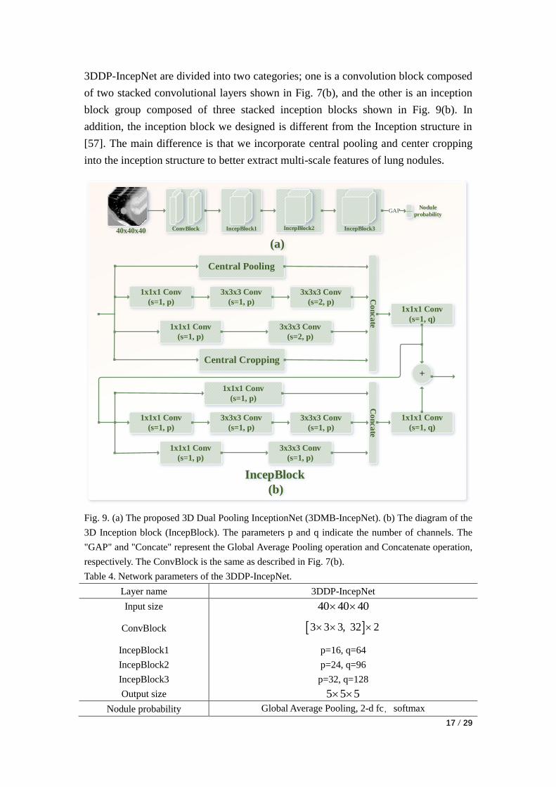
3.2.3. 3D Dual Pooling IncepNet

Fig. 9 shows the architecture of the proposed 3D dual pooling inception network

(3DDP-IncepNet), and Table 4 lists its corresponding network parameters. As shown

in Figure 9, the network contains 41 convolutional layers, three DP layers, and one

global average pooling layer. Among them, the 41 convolutional layers of

17 / 29

3DDP-IncepNet are divided into two categories; one is a convolution block composed

of two stacked convolutional layers shown in Fig. 7(b), and the other is an inception

block group composed of three stacked inception blocks shown in Fig. 9(b). In

addition, the inception block we designed is different from the Inception structure in

[57]. The main difference is that we incorporate central pooling and center cropping

into the inception structure to better extract multi-scale features of lung nodules.

IncepBlock1 IncepBlock3

GAP

ConvBlock

(a)

40x40x40

Nodule

probability

Central Pooling

3x3x3 Conv

(s=2, p)

1x1x1 Conv

(s=1, p)

3x3x3 Conv

(s=1, p)

3x3x3 Conv

(s=2, p)

Co

nca

te

1x1x1 Conv

(s=1, p)

IncepBlock

(b)

1x1x1 Conv

(s=1, q)

1x1x1 Conv

(s=1, p)

3x3x3 Conv

(s=1, p)

1x1x1 Conv

(s=1, p)

3x3x3 Conv

(s=1, p)

3x3x3 Conv

(s=1, p)

Co

nca

te

1x1x1 Conv

(s=1, p)

1x1x1 Conv

(s=1, q)

+

IncepBlock2

Central Cropping

Fig. 9. (a) The proposed 3D Dual Pooling InceptionNet (3DMB-IncepNet). (b) The diagram of the

3D Inception block (IncepBlock). The parameters p and q indicate the number of channels. The

"GAP" and "Concate" represent the Global Average Pooling operation and Concatenate operation,

respectively. The ConvBlock is the same as described in Fig. 7(b).

Table 4. Network parameters of the 3DDP-IncepNet.

Layer name 3DDP-IncepNet

Input size 40 40 40

ConvBlock 3 3 3, 32 2

IncepBlock1 p=16, q=64

IncepBlock2 p=24, q=96

IncepBlock3 p=32, q=128

Output size 5 5 5

Nodule probability Global Average Pooling, 2-d fc，softmax

18 / 29

3.2.4. Random mask

To ensure a high recall rate, when using the segmentation model to search the

candidate nodules in the first stage, it is inevitable that some false positive nodules

will be introduced. In order to ensure the reasonableness of the evaluation results,

when training the false positive reduction model, we only use the candidate nodule

obtained in the first stage as the training sample, and do not use the annotation file

provided by the second track of luna16 (because it contains some samples detected in

the first stage). Even if the sample obtained in the first stage is used to train the false

positive reduction model, there is an imbalance problem on the number of positive

and negative samples. To solve the problem of the imbalance on the number of

positive samples (true lung nodules) and negative samples (blood vessels, lung walls,

lung parenchyma, etc.), we expand the data of positive samples in the training set to

make the ratio of positive and negative samples tends to be 1. Among them, the

expansion method is to rotate the lung nodules by 90°, 180° and 270° on the axial

plane, and to translate one voxel in the X, Y and Z directions. Later, in order to further

improve the generalization ability of the model, we extend the positive and negative

samples in the training set by the random mask data augmentation method.

Specifically, the expansion for positive samples is to randomly select T (5% of the

number of negative samples) samples for the expanded positive and negative samples.

Then, the selected T positive samples and T negative samples are randomly paired;

finally, centering on the nodule, the data patch of size D*D*D (D is the diameter of

the current nodule) is cropped to replace the data patch corresponding to the negative

sample paired with it, thereby converting the negative sample into a new positive

sample. The expansion of the negative samples is relatively simple, that is, only T

samples need to be randomly selected from the positive samples, and then the

corresponding data patch of size D*D*D is set to 0 with the nodule as the center (i.e.,

set the intensity of each voxel in the data patch to 0), so that the T positive samples

are converted into T negative samples.

3.2.5. Training procedure

The training procedure for the three 3D CNN network architectures for false

positive reduction is identical. The SGD optimizer is used to update the model

parameters, and the corresponding initial learning rate is 0.001. After that, each

generation of learning rate decays to 90% of the previous generation learning rate. In

addition, their corresponding total training algebra, batch size, and momentum are 20,

64, and 0.9, respectively. Finally, we maximize the probability of the correct class by

19 / 29

minimizing the cross entropy loss of each training sample. For an input sample given

a positive or negative label, assuming that y is its true label, then the loss function is

defined as shown in equation (5):

1

1[ ( ) (1 ) (1- )]

N

n n n n

n

L y log y y log yN

(5)

where y' is the predicted probability of the model and N is the number of samples.

4. Data and experiment

Below we will further explain the data used and related experiments. The chapter

is divided into three subsections, Section 4.1 describes the data used, Section 4.2

describes the evaluation criteria, and Section 4.3 describes the experimental

environment.

4.1. Data

We used the data set containing 1186 lung nodules provided by the first phase of

LUNA16 (the annotation information includes the diameter and location information

of the nodules) [61]. Furthermore, it should be noted that this dataset is a subset of the

public LIDC-IDRI data set containing 2610 lung nodules. They screened 888 CT data

from the LIDC-IDRI dataset, each of which was labeled by up to four experienced

radiologists [62]. Moreover, each radiologist classifies the identified lesions into three

categories, non-nodular (other tissues or background), nodules larger than 3 mm in

diameter, and nodules less than 3 mm in diameter. Finally, nodules larger than 3 mm

in diameter, marked by three or four radiologists, are used as the gold standard, and

nodules that are less than 3 mm in diameter and marked by only one or two

radiologists will be ignored.

4.2. Evaluation criteria

Our evaluation criteria are the same as those used in the LUNA16 competition.

The competition performance metric (CPM) was defined as the average sensitivity of

seven predefined false positive rates (these seven values are 0.125, 0.25, 0.5, 1, 2, 4,

and 8), and calculated as follows.

{0.125,0.25,0.5,1,2,4,8}

1= fpr i

i

CPM RecallN

(6)

20 / 29

wherein, the value of "N" is seven, "fpr" is the average number of false positives per

scan, and "Recallfpr=i" is the recall rate corresponding to fpr=i.

4.3. Experimental environment

The hardware environment for all our experiments is the server with an Intel(R)

Xeon(R) processor and 125GB of RAM. Moreover, the server has 10 GPUs, the

model is GTX-1080Ti GPU, and the video memory size is 11GB. In addition, the

software environment on which all experiments are based is operating system ubuntu

14.04, integrated development tool PyCharm 2017.2.1, coding language Python 3.6.4,

deep learning framework Keras. According to our experiments, the time required for

the 3DDP-SeResNet, 3DDP-DenseNet and 3DDP-IncepNet models to converge was

approximately 18, 16 and 13 hours, respectively.

5. Results and discussion

This section is divided into three subsections, of which Section 5.1 describes the

overall performance of the proposed method, Section 5.2 describes the ablation study

of the proposed method, and Section 5.3 describes our comparative experiment.

5.1. Overall performance

To more intuitively observe the overall performance of the proposed false

positive reduction method, we plot the FROC curves for 3DDP-DenseNet,

3DDP-SeResNet and 3DMB-InceptionNet, and their integrated corresponding FROC

curves in Fig. 10. In these three networks, when the false positive rate of each scan is

1, the corresponding sensitivity can reach more than 90%; their integration results in a

false positive rate of 0.25, the corresponding sensitivity reached 90%, which indicates

that the network architecture based on 3D CNN can adapt to the classification of true

and false lung nodules to some extent.

Table 5 lists the quantitative metrics for the three independent network

architectures, namely the sensitivity at the different false alarm rates specified in the

Challenge. As can be seen from Table 5, when the false positive rate of each scan is

0.125, the recall rates of the three networks proposed are less than 80%, and their

integration corresponds to the sensitivity of 84.8%, which is compared with

3DDP-IncepNet-RDU increased by 15.8 percentage points. At this extremely low

false positive rate, our multi-model integration strategy has shown satisfactory results.

21 / 29

Even for the final CPM score, the integrated result is 2.5 percentage points higher

than the best-performing 3DDP-SeResNet-RDU. These experiments show that

different network architectures can complement each other's defects, and their

integration can improve the performance.

Fig. 10. FROC curves for the three networks and their integration.

Table 5. The sensitivities of models under different false positive rates. Note that, RDU indicates

ResDense-based UNet architecture and uses the proposed sampling strategy to train the

segmentation model.

Method 0.125 0.25 0.5 1 2 4 8 CPM

3DDP-DenseNet-RDU 0.768 0.830 0.877 0.931 0.950 0.951 0.960 0.895

3DDP-SeResNet-RDU 0.730 0.849 0.916 0.929 0.948 0.958 0.958 0.900

3DDP-IncepNet-RDU 0.686 0.833 0.891 0.921 0.942 0.949 0.955 0.883

TSCNN 0.848 0.900 0.925 0.936 0.949 0.957 0.960 0.925

5.2. Ablation study

To validate the effectiveness of the various components in the TSCNN

architecture, we designed a 2D DenseNet-based ablation experiment. The results are

shown in Table 6. It should be noted that in order to shorten the length, we only

randomly select one fold for the ablation experiment, and the other tables show the

results of the 10-fold cross-validation (except Tables 8, 9 and 10). In addition, the first

four rows in Table 6 (except the header) verify the validity of the components in the

proposed segmentation network, and the last seven rows verify the validity of the

components in the proposed classification network. This will be explained below.

22 / 29

(1) The effectiveness of the sample selection

Comparing the first two rows of Table 6, it can be found that in the case of using

2D DenseNet for false positive reduction, the CPM score corresponding to the

weighted sampling strategy [58] is 0.546, and the CPM score corresponding to the

proposed sampling strategy is 0.563. The proposed sampling strategy increased

performance by 1.7 percentage points, which validated the effectiveness of our

proposed sampling strategy.

(2) The effectiveness of the basic structure

Comparing the second and third rows of Table 6, we can find that the UNet

network model based on ResDense structure is 1.2% higher than the original UNet

network architecture [63]. Especially, when the false positive rate is 0.125, the

corresponding recall rate is particularly effective, which is 4.6 percentage points

higher than the original UNet structure. This illustrates that the segmentation model

based on ResDense structure is effective.

(3) The effectiveness of the hard mining

Comparing the third and fourth rows of Table 6, we can find that the

segmentation model is trained based on the idea of offline hard Mining. Although the

corresponding recall rate was lower than the conventional training method when the

false positive rate was 0.125 and 0.25, the overall performance was improved by 2

percentage points. In general, the segmentation model based on HM idea training is

acceptable.

(4) Effect of the dimensional space

As can be seen from the 4th and 5th rows of Table 6, in the case of ensuring that

the same segmentation model is used, the classification model based on 2D DenseNet

has a CPM score of 0.595, and the classification model based on 3D DenseNet has a

CPM score of 0.835. By comparing these two results, it can be found that the

classification model based on 3D DenseNet improves the performance by 24%.

Although the model parameters are increased (3D DenseNet's trainable model

parameters are three times that of 2D DenseNet), the performance is greatly improved,

which verifies the effectiveness by using more spatial information.

(5) The effectiveness of the downsampling method

Comparing 5th and 6th rows of Table 6, it can be seen that the downsampling

method based on the central pooling is slightly better than the traditional max pooling

method. After we combine the central pooling with the center cropping to form the

dual pooling for downsampling, the performance is greatly improved (the result

corresponds to line 7 of Table 6). Compared with the traditional max pooling, the

23 / 29

CPM score increased by 3.6 percentage points, which verified the effectiveness of the

dual pooling of our design in our experiments.

(6) The effectiveness of the random mask

Comparing 7th and 8th rows of Table 6, it can be seen that after using the

proposed data augmentation method based on random mask, the recall rate

corresponding to the seven false positive rates was improved compared to the results

in row 7 of Table 6. Although the final CPM score improvement effect is not

significant (false positive rate 0.125 corresponding recall rate improvement effect is

more obvious), but also 1.1 percentage points increase, which to some extent also

verified the effectiveness of the proposed random mask based data augmentation

method.

In addition, the effectiveness of ensemble learning can also be verified by

comparing the last four lines of Table 6.

Table 6. Ablation experiment. Note that, "2DDNet" indicates the 2D-DenseNet; "MP" indicates

max pooling; "WSS" represents weighted sampling strategy[58]; "PSS" represents the proposed

sampling strategy; "HM" represents the hard mining operation, see section 3.1.3; "CP" indicates

central pooling; "DP" represents the combination of central pooling and central cropping; "RM"

represents the data enhancement strategy based on random mask. In addition, for the convenience

of writing in Table 6, we have abbreviated "3D-DenseNet", "3D-SeResNet" and "3D-IncepNet" as

"3DDNet", "3DSNet" and "3DINet", respectively.

Method 0.125 0.25 0.5 1 2 4 8 CPM

2DDNet_MP-UNet_WSS 0.308 0.398 0.491 0.549 0.642 0.688 0.748 0.546

2DDNet_MP-UNet_PSS 0.347 0.405 0.463 0.548 0.651 0.761 0.768 0.563

2DDNet_MP-RDU 0.393 0.426 0.465 0.568 0.656 0.725 0.793 0.575

2DDNet_MP-RDU_HM 0.262 0.379 0.480 0.625 0.750 0.801 0.866 0.595

3DDNet_MP-RDU_HM 0.583 0.769 0.833 0.883 0.914 0.931 0.932 0.835

3DDNet_CP-RDU_HM 0.654 0.748 0.835 0.882 0.912 0.916 0.931 0.840

3DDNet_DP-RDU_HM 0.745 0.822 0.872 0.902 0.916 0.916 0.926 0.871

3DDNet_DP_RM-RDU_HM 0.774 0.837 0.877 0.910 0.916 0.929 0.931 0.882

3DSNet_DP_RM-RDU_HM 0.703 0.855 0.910 0.912 0.925 0.928 0.928 0.880

3DINet_DP_RM-RDU_HM 0.730 0.846 0.877 0.898 0.923 0.934 0.934 0.877

TSCNN 0.868 0.900 0.913 0.915 0.916 0.931 0.932 0.911

5.3. Experimental comparison

To verify the effectiveness of the proposed methods, we compared them with the

nodule detection approaches published in recent years. Table 7 shows the quantitative

results in the comparison of traditional detection methods, machine learning based

detection methods, and CNN-based detection methods. It can be seen from Table 7

24 / 29

that although the detection methods based on the nodule enhancement filter and the

support vector machine proposed by Teramoto et al. [24] are not effective, the

machine learning-based detection methods and CNN-based detection methods are

generally superior to traditional detection methods. In addition, for traditional

machine learning-based detection methods and CNN-based detection methods, we

believe that CNN-based deep learning methods are more scalable and robust.

Generally speaking, some machine learning-based detection methods have achieved

good results. For example, Liu et al. [25] and Javaid et al. [21] proposed methods

based on traditional machine learning algorithm for lung nodule detection, but they

need to manually design related features for later classification, which greatly limits

the scalability of the method. However, the CNN-based approach is more natural,

which automatically learns advanced semantic features through training. The methods

we proposed are based on the CNN. By comparing the experimental results in Table 7,

it is competitive with existing lung nodule detection methods.

Table 7. A comparison on the quantitative results of various false positive reduction methods.

Among them, "Ours" indicates the result of the 10-fold cross-validation of our proposed method.

Please note that, "TA" indicates the traditional algorithm, "ML" indicates the machine learning,

and "CNN" indicates the convolution neural networks. In addition, "V-fps=n" means that when there

are n false positives per scan, the corresponding recall rate is smaller than the value V. For

example, the corresponding results of El-Regaily (V=0.705-, n=4) indicate that when there are 4

false positives per scan, the corresponding recall rate is less than or equal to 0.705 (The original

paper [15] only shows that when there are 4.1 false positives per scan, the corresponding recall

rate is 0.705).

Type Method 0.125 0.25 0.5 1 2 4 8 CPM

TA

El-Regaily [15] * * * * * 0.705- * *

Anoop [16] * * * * * 0.850- * *

Lu [19] * * * * 0.852- * * *

Wang [12] * * * * * 0.880 * *

ML

Liu [23] * * * 0.893- * * * *

Teramoto [24] * * * * * * 0.830- *

Liu [25] * * * * * 0.948- * *

Javaid [21] * * * * 0.917- * * *

CNN

Hamidian [47] 0.583 0.687 0.742 0.828 0.886 0.918 0.933 0.797

Xie [37] 0.734 0.744 0.763 0.796 0.824 0.832 0.834 0.790

Dou [38] 0.659 0.745 0.819 0.865 0.906 0.933 0.946 0.839

Zhu [45] * * * * * * * 0.842

Ding [46] * * * * * * * 0.891

Khosravan [50] * * * * * * * 0.897

CNN Ours 0.848 0.899 0.925 0.936 0.949 0.957 0.960 0.925

25 / 29

6. Conclusion

In this study, we designed a two-stage convolutional neural network architecture

to better detect lung nodules. In general, we first use the proposed UNet segmentation

model based on ResDense structure to search suspicious nodules (the centroid of the

segmented mask is the location of the suspected lung nodules), and then use the

proposed 3D CNN-based ensemble learning architecture to eliminate false positive

nodules. In addition, we verified each component and overall performance of the

proposed lung nodule detection method by ablation study and experimental

comparison. According to the experimental results shown in Tables 6 and 7, we can

see that our results are competitive compared to other existing technical methods.

Acknowledgements

The National Key R&D Program of China (Grant No. 2017YFC0112804) and the

National Natural Science Foundation of China (Grant No. 81671768) supported this

work. The authors acknowledge the National Cancer Institute and the Foundation for

the National Institutes of Health and their critical role in the creation of the free

publicly available LIDC-IDRI Database used in this study.

Reference

[1] J. Ferlay, I. Soerjomataram, R. Dikshit, S. Eser, C. Mathers, M. Rebelo, et al., "Cancer

incidence and mortality worldwide: sources, methods and major patterns in GLOBOCAN

2012," International journal of cancer, vol. 136, pp. E359-86, 2015/03// 2015.

[2] K. Bhavanishankar and M. V. Sudhamani, "Techniques for Detection of Solitary Pulmonary

Nodules in Human Lung and Their Classifications -A Survey," vol. 4, pp. 27-40, 2015.

[3] R. L. Siegel, K. D. Miller, and A. Jemal, "Cancer statistics, 2018," CA: a cancer journal for

clinicians, vol. 68, pp. 7-30, 2018/01// 2018.

[4] D. R. Baldwin, "Prediction of risk of lung cancer in populations and in pulmonary nodules:

Significant progress to drive changes in paradigms," Lung cancer (Amsterdam, Netherlands),

vol. 89, pp. 1-3, 2015/07// 2015.

[5] H. J. W. L. Aerts, E. R. Velazquez, R. T. H. Leijenaar, C. Parmar, P. Grossmann, S. Carvalho,

et al. (2014, 2014/06//). Decoding tumour phenotype by noninvasive imaging using a

quantitative radiomics approach. Nature communications 5, 4006.

[6] I. R. S. Valente, P. C. Cortez, E. C. Neto, J. M. Soares, V. H. C. de Albuquerque, and J. M. R.

S. Tavares, "Automatic 3D pulmonary nodule detection in CT images: A survey," Computer

methods and programs in biomedicine, vol. 124, pp. 91-107, 2016/02// 2016.

26 / 29

[7] M. Zia ur Rehman, M. Javaid, S. I. A. Shah, S. O. Gilani, M. Jamil, and S. I. Butt, "An

appraisal of nodules detection techniques for lung cancer in CT images," Biomedical Signal

Processing and Control, vol. 41, pp. 140-151, 2018/03/01/ 2018.

[8] J. Zhang, Y. Xia, H. Cui, and Y. Zhang, "Pulmonary nodule detection in medical images: A

survey," Biomedical Signal Processing and Control, vol. 43, pp. 138-147, 2018/05/01/ 2018.

[9] W. Zhang, X. Wang, X. Li, and J. Chen, "3D skeletonization feature based computer-aided

detection system for pulmonary nodules in CT datasets," Computers in Biology and Medicine,

vol. 92, pp. 64-72, 2018/01/01/ 2018.

[10] Y. Chen, C. Liu, W. Peng, and S. Xia, "Thyroid nodule detection using attenuation value based

on non-enhancement CT images," in 2nd IET International Conference on Biomedical Image

and Signal Processing (ICBISP 2017), 2017, pp. 1-4.

[11] M. P. Paing and S. Choomchuay, "A computer aided diagnosis system for detection of lung

nodules from series of CT slices," in 2017 14th International Conference on Electrical

Engineering/Electronics, Computer, Telecommunications and Information Technology

(ECTI-CON), 2017, pp. 302-305.

[12] B. Wang, X. Tian, Q. Wang, Y. Yang, H. Xie, S. Zhang, et al., "Pulmonary nodule detection in

CT images based on shape constraint CV model," Medical Physics, vol. 42, p. 1241, 2015.

[13] T. Messay, R. C. Hardie, and S. K. Rogers, "A new computationally efficient CAD system for

pulmonary nodule detection in CT imagery," Medical image analysis, vol. 14, pp. 390-406,

2010/06// 2010.

[14] J. John and M. G. Mini, "Multilevel Thresholding Based Segmentation and Feature Extraction

for Pulmonary Nodule Detection," Procedia Technology, vol. 24, pp. 957-963, 2016/01/01/

2016.

[15] S. A. El-Regaily, M. A. M. Salem, M. H. A. Aziz, and M. I. Roushdy, "Lung nodule

segmentation and detection in computed tomography," in 2017 Eighth International

Conference on Intelligent Computing and Information Systems (ICICIS), 2017, pp. 72-78.

[16] C. S. Anoop and V. Preeja, "Lung Nodule Detection and Analysis using VDE Chest

Radiographs," International Journal of Computer Applications, vol. 115, pp. 31-36, 2015.

[17] A. Gupta, O. Martens, Y. L. Moullec, and T. Saar, "Methods for increased sensitivity and

scope in automatic segmentation and detection of lung nodules in CT images," in 2015 IEEE

International Symposium on Signal Processing and Information Technology (ISSPIT), 2015,

pp. 375-380.

[18] A. A. Rezaie and A. Habiboghli, "Detection of Lung Nodules on Medical Images by the Use

of Fractal Segmentation," IJIMAI, vol. 4, pp. 15-19, 2017.

[19] L. Lu, Y. Tan, L. H. Schwartz, and B. Zhao, "Hybrid detection of lung nodules on CT scan

images," Medical Physics, vol. 42, pp. 5042-5054, 2015.

[20] G. Aresta, A. Cunha, and A. Campilho, "Detection of juxta-pleural lung nodules in computed

tomography images," in Society of Photo-Optical Instrumentation Engineers, 2017, p.

101343N.

[21] M. Javaid, M. Javid, M. Z. U. Rehman, and S. I. A. Shah, "A novel approach to CAD system

for the detection of lung nodules in CT images," Computer methods and programs in

biomedicine, vol. 135, pp. 125-139, 2016/10// 2016.

[22] A. O. d. C. Filho, A. C. Silva, A. C. de Paiva, R. A. Nunes, and M. Gattass, "3D shape analysis

to reduce false positives for lung nodule detection systems," Medical & Biological

27 / 29

Engineering & Computing, vol. 55, pp. 1199-1213, 2017/08/01 2017.

[23] Y. Liu, Z. Wang, M. Guo, and P. Li, "Hidden conditional random field for lung nodule

detection," in 2014 IEEE International Conference on Image Processing (ICIP), 2014, pp.

3518-3521.

[24] A. Teramoto and H. Fujita, "Automated Lung Nodule Detection Using Positron Emission

Tomography/Computed Tomography," in Artificial Intelligence in Decision Support Systems

for Diagnosis in Medical Imaging, K. Suzuki and Y. Chen, Eds., ed Cham: Springer

International Publishing, 2018, pp. 87-110.

[25] J.-k. Liu, H.-y. Jiang, M.-d. Gao, C.-g. He, Y. Wang, P. Wang, et al., "An Assisted Diagnosis

System for Detection of Early Pulmonary Nodule in Computed Tomography Images," Journal

of Medical Systems, vol. 41, p. 30, 2016/12/28 2016.

[26] B. R. Froz, A. O. D. C. Filho, A. C. Silva, A. C. D. Paiva, R. A. Nunes, and M. Gattass, "Lung

nodule classification using artificial crawlers, directional texture and support vector machine,"

Expert Systems with Applications, vol. 69, pp. 176-188, 2017.

[27] E. Aghabalaei Khordehchi, A. Ayatollahi, and M. R. Daliri, "AUTOMATIC LUNG NODULE

DETECTION BASED ON STATISTICAL REGION MERGING AND SUPPORT VECTOR

MACHINES," 2017, vol. 36, p. 14, 2017-06-23 2017.

[28] E. E. Nithila and S. S. Kumar, "Automatic detection of solitary pulmonary nodules using

swarm intelligence optimized neural networks on CT images," Engineering Science and

Technology, an International Journal, vol. 20, pp. 1192-1202, 2017/06/01/ 2017.

[29] M. Alam, G. Sankaranarayanan, and V. Devarajan, "Lung Nodule Detection and Segmentation

Using a Patch-Based Multi-Atlas Method," in 2016 International Conference on

Computational Science and Computational Intelligence (CSCI), 2016, pp. 23-28.

[30] N. Tajbakhsh and K. Suzuki, "Comparing two classes of end-to-end machine-learning models

in lung nodule detection and classification: MTANNs vs. CNNs," Pattern Recognition, vol. 63,

pp. 476-486, 2017/03/01/ 2017.

[31] K.-L. Hua, C.-H. Hsu, S. C. Hidayati, W.-H. Cheng, and Y.-J. Chen. (2015, 2015).

Computer-aided classification of lung nodules on computed tomography images via deep

learning technique. OncoTargets and therapy 8, 2015-2022.

[32] H. Jiang, H. Ma, W. Qian, M. Gao, and Y. Li, "An Automatic Detection System of Lung

Nodule Based on Multi-Group Patch-Based Deep Learning Network," IEEE Journal of

Biomedical and Health Informatics, vol. PP, pp. 1-11, 2017.

[33] W. Li, P. Cao, D. Zhao, and J. Wang, "Pulmonary Nodule Classification with Deep

Convolutional Neural Networks on Computed Tomography Images," Computational and

mathematical methods in medicine, vol. 2016, p. 6215085, 2016.

[34] B. v. Ginneken, A. A. A. Setio, C. Jacobs, and F. Ciompi, "Off-the-shelf convolutional neural

network features for pulmonary nodule detection in computed tomography scans," in 2015

IEEE 12th International Symposium on Biomedical Imaging (ISBI), 2015, pp. 286-289.

[35] L. Fu, J. Ma, Y. Ren, Y. S. Han, and J. Zhao, "Automatic detection of lung nodules: false

positive reduction using convolution neural networks and handcrafted features," Proceedings

of the Spie, vol. 134, p. 101340A, 2017.

[36] H. C. Shin, H. R. Roth, M. Gao, L. Lu, Z. Xu, I. Nogues, et al., "Deep Convolutional Neural

Networks for Computer-Aided Detection: CNN Architectures, Dataset Characteristics and

Transfer Learning," IEEE Transactions on Medical Imaging, vol. 35, pp. 1285-1298, 2016.

28 / 29

[37] H. Xie, D. Yang, N. Sun, Z. Chen, and Y. Zhang, "Automated pulmonary nodule detection in

CT images using deep convolutional neural networks," Pattern Recognition, vol. 85, pp.

109-119, 2019/01/01/ 2019.

[38] Q. Dou, H. Chen, Y. Jin, H. Lin, J. Qin, and P.-A. Heng, "Automated Pulmonary Nodule

Detection via 3D ConvNets with Online Sample Filtering and Hybrid-Loss Residual

Learning," in Medical Image Computing and Computer-Assisted Intervention − MICCAI

2017, Cham, 2017, pp. 630-638.

[39] F. Ciompi, B. de Hoop, S. J. van Riel, K. Chung, E. T. Scholten, M. Oudkerk, et al.,

"Automatic classification of pulmonary peri-fissural nodules in computed tomography using

an ensemble of 2D views and a convolutional neural network out-of-the-box," Medical image

analysis, vol. 26, pp. 195-202, 2015/12// 2015.

[40] A. A. A. Setio, F. Ciompi, G. Litjens, P. Gerke, C. Jacobs, S. J. v. Riel, et al., "Pulmonary

Nodule Detection in CT Images: False Positive Reduction Using Multi-View Convolutional

Networks," IEEE Transactions on Medical Imaging, vol. 35, pp. 1160-1169, 2016.

[41] S. R. S., J. George, S. Skaria, and V. V. V., "Using YOLO based deep learning network for real

time detection and localization of lung nodules from low dose CT scans," in SPIE Medical

Imaging, 2018, p. 9.

[42] W. Zhu, C. Liu, W. Fan, and X. Xie, "DeepLung: 3D Deep Convolutional Nets for Automated

Pulmonary Nodule Detection and Classification," bioRxiv, 2017.

[43] X. Huang, J. Shan, and V. Vaidya, "Lung nodule detection in CT using 3D convolutional

neural networks," in 2017 IEEE 14th International Symposium on Biomedical Imaging (ISBI

2017), 2017, pp. 379-383.

[44] W. Zhu, Y. S. Vang, Y. Huang, and X. Xie, "DeepEM: Deep 3D ConvNets With EM For

Weakly Supervised Pulmonary Nodule Detection," CoRR, vol. abs/1805.05373, / 2018.

[45] W. Zhu, C. Liu, W. Fan, and X. Xie, "DeepLung: Deep 3D Dual Path Nets for Automated

Pulmonary Nodule Detection and Classification," in 2018 IEEE Winter Conference on

Applications of Computer Vision (WACV), 2018, pp. 673-681.

[46] J. Ding, A. Li, Z. Hu, and L. Wang, "Accurate Pulmonary Nodule Detection in Computed

Tomography Images Using Deep Convolutional Neural Networks," in Medical Image

Computing and Computer-Assisted Intervention − MICCAI 2017, Cham, 2017, pp. 559-567.

[47] S. Hamidian, B. Sahiner, N. Petrick, and A. Pezeshk, "3D Convolutional Neural Network for

Automatic Detection of Lung Nodules in Chest CT," in SPIE Medical Imaging, 2017, p.

1013409.

[48] H. Tang, D. R. Kim, and X. Xie, "Automated pulmonary nodule detection using 3D deep

convolutional neural networks," in 2018 IEEE 15th International Symposium on Biomedical

Imaging (ISBI 2018), 2018, pp. 523-526.

[49] N. M. Jenuwine, S. N. Mahesh, J. D. Furst, and D. S. Raicu, "Lung nodule detection from CT

scans using 3D convolutional neural networks without candidate selection," in SPIE Medical

Imaging, 2018, p. 8.

[50] N. Khosravan and U. Bagci, "S4ND: Single-Shot Single-Scale Lung Nodule Detection," in

Medical Image Computing and Computer Assisted Intervention – MICCAI 2018, Cham, 2018,

pp. 794-802.

[51] H. Cao, H. Liu, and E. Song, "A novel algorithm for segmentation of leukocytes in peripheral

blood," Biomedical Signal Processing and Control, vol. 45, pp. 10-21, 2018/08/01/ 2018.

29 / 29

[52] D. P. Kingma and J. Ba, "Adam: A Method for Stochastic Optimization," CoRR, vol.

abs/1412.6980, / 2014.

[53] R. Caruana, S. Lawrence, and C. L. Giles, "Overfitting in Neural Nets: Backpropagation,

Conjugate Gradient, and Early Stopping," 2000.

[54] F. Milletari, N. Navab, and S. A. Ahmadi, "V-Net: Fully Convolutional Neural Networks for

Volumetric Medical Image Segmentation," in 2016 Fourth International Conference on 3D

Vision (3DV), 2016, pp. 565-571.

[55] J. Hu, L. Shen, and G. Sun, "Squeeze-and-Excitation Networks," CoRR, vol. abs/1709.01507,

/ 2017.

[56] G. Huang, Z. Liu, L. v. d. Maaten, and K. Q. Weinberger, "Densely Connected Convolutional

Networks," in 2017 IEEE Conference on Computer Vision and Pattern Recognition (CVPR),

2017, pp. 2261-2269.

[57] C. Szegedy, S. Ioffe, V. Vanhoucke, and A. A. Alemi, "Inception-v4, Inception-ResNet and the

Impact of Residual Connections on Learning," 2017.

[58] S. Wang, M. Zhou, Z. Liu, Z. Liu, D. Gu, Y. Zang, et al., "Central focused convolutional

neural networks: Developing a data-driven model for lung nodule segmentation," Medical

Image Analysis, vol. 40, pp. 172-183, 2017/08/01/ 2017.

[59] S. Ioffe and C. Szegedy, "Batch Normalization: Accelerating Deep Network Training by

Reducing Internal Covariate Shift," 2015, pp. 448-456.

[60] K. He, X. Zhang, S. Ren, and J. Sun, "Delving Deep into Rectifiers: Surpassing Human-Level

Performance on ImageNet Classification," in 2015 IEEE International Conference on

Computer Vision (ICCV), 2015, pp. 1026-1034.

[61] A. A. A. Setio, A. Traverso, T. de Bel, M. S. N. Berens, C. v. d. Bogaard, P. Cerello, et al.,

"Validation, comparison, and combination of algorithms for automatic detection of pulmonary

nodules in computed tomography images: The LUNA16 challenge," Medical Image Analysis,

vol. 42, pp. 1-13, 2017/12/01/ 2017.

[62] S. G. Armato, G. McLennan, L. Bidaut, M. F. McNitt-Gray, C. R. Meyer, A. P. Reeves, et al.,

"The Lung Image Database Consortium (LIDC) and Image Database Resource Initiative

(IDRI): a completed reference database of lung nodules on CT scans," Medical physics, vol.

38, pp. 915-931, 2011/02// 2011.

[63] O. Ronneberger, P. Fischer, and T. Brox, "U-Net: Convolutional Networks for Biomedical

Image Segmentation," in Medical Image Computing and Computer-Assisted Intervention –

MICCAI 2015, Cham, 2015, pp. 234-241.