35
Type-Compatible Equilibria in Signalling Games Drew Fudenberg Kevin He November 15, 2016
| Date post: | 31-Jul-2018 |
| Category: |
Documents |
| Upload: | nguyenduong |
| View: | 214 times |
| Download: | 0 times |
Type-Compatible Equilibria in Signalling Games
Drew FudenbergKevin He
November 15, 2016
Motivation
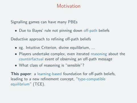
Signalling games can have many PBEs
• Due to Bayes’ rule not pinning down off-path beliefs
Deductive approach to refining off-path beliefs
• eg. Intuitive Criterion, divine equilibrium, ...• Players undertake complex, even iterated reasoning about thecounterfactual event of observing an off-path message• What class of reasoning is “sensible”?
This paper: a learning-based foundation for off-path beliefs,leading to a new refinement concept, “type-compatibleequilibrium” (TCE).
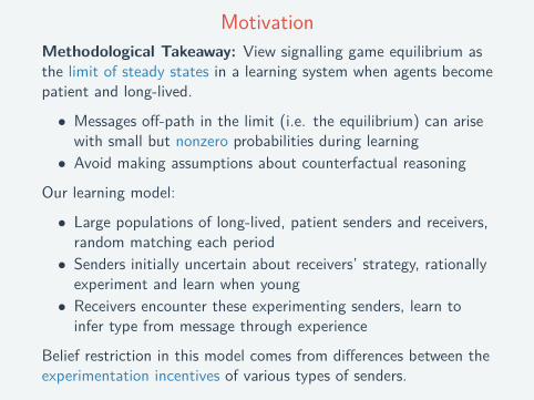
MotivationMethodological Takeaway: View signalling game equilibrium asthe limit of steady states in a learning system when agents becomepatient and long-lived.
• Messages off-path in the limit (i.e. the equilibrium) can arisewith small but nonzero probabilities during learning• Avoid making assumptions about counterfactual reasoning
Our learning model:
• Large populations of long-lived, patient senders and receivers,random matching each period• Senders initially uncertain about receivers’ strategy, rationallyexperiment and learn when young• Receivers encounter these experimenting senders, learn toinfer type from message through experience
Belief restriction in this model comes from differences between theexperimentation incentives of various types of senders.

Related LiteratureSignalling-game refinements• Cho and Kreps (1987): Intuitive Criterion, D1• Banks and Sobel (1987): divine equilibrium, universal divinity
Learning in games• Heuristic experimentation:
I Fudenberg and Kreps (1993, 1995): asymptotically myopicactions, exogenously assumed restrictions on experimentation
I Jehiel and Samet (2005): pick move with highest “valuation”I Laslier and Walliser (2014): compare payoffs in past two
periods, then change strategy by ±1• Rational experimentation:
I Kalai and Lehrer (1993): Bayesian learning with grain of truthI Fudenberg and Levine (1993, 2006): steady state learning
Techniques and tools• Gittins and Jones (1974), Gittins (1979): the Gittins index• Fudenberg, He, and Imhof (2016)
I New results on Bayesian posteriors after rare events

Outline
1. Type-Compatible Equilibrium1.1 Definition1.2 Main Theorem: “only TCEs can be learning outcomes for
patient, long-lived agents”1.3 Some Intuitions
2. Steady State Learning Model3. Proof Sketch of the Main Theorem4. A Diagram

1. Type-Compatible Equilibrium

Notation for Signalling Game
• Finite set of types for the sender, Θ• Type distribution λ ∈ ∆(Θ) so that λ(θ) > 0 for all θ ∈ Θ• Finite set of messages for the sender, M• Finite set of actions for the receiver, A• Utility functions uS , uR : Θ×M × A→ R• Behavioral strategies [πS(·|θ)]θ∈Θ, [πR(·|m)]m∈M

Notation for Signalling Game
• For P ⊆ ∆(Θ), BR(P,m) ⊆ A is the set of best response tom supported by some belief in P,
BR(P,m) :=⋃
p∈P
(argmax
a′∈AuR(p,m, a′)
)
• ΠR := receiver strategies πR such thatπR(·|m) ∈ ∆(BR(Θ),m) for each m• UD(θ): undominated messages for type θ, best responseagainst some belief about receiver’s strategy• ΠS := ×θ∆(UD(θ))

Compatibility
Definition (θ′ �m′ θ′′)
θ′ is more compatible with m′ than θ′′ if for every πR ∈ ΠR ,
uS(θ′′,m′
, πR) ≥ maxm′′ 6=m′
uS(θ′′,m′′
, πR)
⇓
uS(θ′,m′
, πR) > maxm′′ 6=m′
uS(θ′,m′′
, πR)
That is, m′ weakly optimal for θ′′ =⇒ m′ strictly optimal for θ′ .
Compatibility is invariant to re-scaling sender’s payoffs.
�m′ is asymmetric except in corner cases: m′ is strictly dominatedfor both types, or m′ is strictly dominant for both types.

A Sufficient Condition for CompatibilityAssume separable sender payoffs uS(θ,m, a) = v(θ,m) + z(a)
• v(θ,m) is type θ’s payoff from message m• z(a) is, eg. a monetary transfer
v(θ′,m′)−v(θ′′,m′) > maxm′′ 6=m′
v(θ′,m′′)−v(θ′′,m′′) =⇒ θ′ �m′ θ′′
It suffices that m′ is the least costly message for θ′ relative to θ′′ .In the beer-quiche game...
• v(strong, beer) = v(weak,quiche) = 1• v(strong, quiche) = v(weak,beer) = 0• z(no fight) = 2, z(fight) = 0• Therefore, strong �beer weak

Type-Compatible Equilibrium
Types who could possibly gain by deviating from π∗S(·|θ) to m′ :
J(m′, π∗) :=
{θ ∈ Θ : max
a∈BR(∆(Θ),m′ )uS(θ,m′
, a) > uS(θ;π∗)}
Compatible beliefs at message m′ under profile π∗:
P(m′, π∗) :=
p ∈ ∆(UD−1(m′)) : p(θ′′ )
p(θ′ ) ≤λ(θ′′ )λ(θ′ ) if
(i) θ′�m′ θ
′′
and
(ii) θ′∈ J(m
′, π∗)
I An illustration

Type-Compatible Equilibrium
Definition
Strategy profile π∗ is a type-compatible equilibrium (TCE) if it is aNash equilibrium and satisfies the compatibility criterion (CC):
π∗R(·|m) ∈ ∆(BR(P(m, π∗),m)) for every m ∈ M.

TCE in the Beer-Quiche Game
beer fight no fightstrong 1,0 3,1weak 0,1 2,0
quiche fight no fightstrong 0,0 2,1weak 1,1 3,0
type distribution λ(strong) = 0.9
• Consider π∗, the PBE of pooling on quiche. Sustained byπ∗R(fight|beer) ≥ 1
2• Showed before: strong �beer weak• Also, strong ∈ J(beer, π∗)• =⇒ P(beer, π∗) =
{p ∈ ∆(Θ) : p(weak)
p(strong) ≤λ(weak)λ(strong) = 1
9
}• But against any p ∈ P(beer, π∗), “no fight” is a strict BR• So π∗ is not a TCE

Learning and TCE• Second half of this talk: a learning model• Signalling game equilibria = (limits of) steady states of thisnon-equilibrium adjustment process
Theorem (informal)
Every learning outcome with patient, long-lived agents is a TCE.
It is easy to prove that:
Proposition (PBE and compatibility criterion)
If π∗ is a PBE, then θ′ �m′ θ′′ =⇒ π∗S(m′ |θ′) ≥ π∗S(m′ |θ′′).
• Bayes’ rule =⇒ CC holds if π∗S(m′ |θ′) > 0.• TCE requires same belief restriction at off-path messages
I Comes from rational experimentation

Intuition for TCE
• Suppose type θ uncertain about π∗R• Each day, send m, observe one draw of π∗R(·|m), get payoffs• Maximize expected β-discounted utility, β ∈ [0, 1)• This is a multi-armed bandit problem (!)• Optimal: choose arm (message) with highest Gittins index,
I(m) = supτ>0
{E[τ−1∑t=0
βtum(t)]/ E
[τ−1∑t=0
βt]}

Intuition for TCE
Proposition (�m′ and the Gittins index)
If θ′ �m′ θ′′ and types have the same beliefs, then m′ has the
highest Gittins index for θ′ whenever it has the highest index for θ′′.
Proof outline:
• Given prior, stopping time τ for m′ induces a distribution over(expected discounted) receiver actions before stopping.• View this distribution as a mixed strategy of the receiver
I Evaluating the optimal stopping problem in the defn. ofGittins index at τ gets sender’s one-period payoff against thereceiver strategy induced by τ
• If θ′ and θ′′ share same beliefs, can apply definition of �m′

2. Steady State Learning Model

Learning Model: Aggregate System
• Continuum of agentsI unit mass of receiversI mass λ(θ) of type-θ senders.
• Time is doubly infinite and generations overlap• In every period...
I each existing agent has γ ∈ [0, 1) chance of surviving, else exitsI (1− γ) new receivers, λ(θ)(1− γ) new type-θ senders are bornI sender learns type upon birth, which is fixed for life

Learning Model: Individual’s Problem• Every period, each agent randomly matched with an agent inthe opposite role and the pair plays the signalling game
I Age or past experience of opponents not observedI At the end of the period, each agent observes the type and
message of the sender, the action of the receiverI Sender does not observe receiver’s extensive-form strategy
• Steady state learning: each agent believes opponentpopulation playing an unknown, stationary strategy• Each agent born with a prior, independent across θ’s or m’s
receiver: gR = ×θ∈Θ
g (θ)R on ΠS
sender: gS = ×m∈M
g (m)S on ΠR
• Assume gR , gS “regular”: continuous, positive on interior,does not vanish to 0 “too fast” at the boundary. Satisfied byDirichlet priors and priors with densities bounded away from 0.
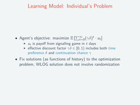
Learning Model: Individual’s Problem
• Agent’s objective: maximize E [∑∞
t=0(γδ)t · ut ]I ut is payoff from signalling game in t daysI effective discount factor γδ ∈ [0, 1) includes both time
preference δ and continuation chance γ• Fix solutions (as functions of history) to the optimizationproblem, WLOG solution does not involve randomization

States of the Learning Model
• A state ψ is a distribution over histories that agents have seen• The fixed (deterministic) solutions to the dynamicoptimization problems generate a deterministic map f fromstate today to state tomorrow• Call ψ∗ a steady state if f (ψ∗) = ψ∗
• Ψ∗(g , δ, γ) := set of steady states under regular priorg = (gS , gR), patience δ, survival chance γ
Proposition
Ψ∗(g , δ, γ) is non-empty and compact.

Patiently Stable Strategy Profiles
• State ψ induces a strategy profile of the signalling game,(ψ̄S , ψ̄R)• Want to characterize strategy profiles associated with
“ limδ→1
limγ→1
” Ψ∗(g , δ, γ)
• Strategy profile π∗ is patiently stable if associated with abovelimit for some regular prior g
I patiently stable strategies exist by previous PropositionI Interpretation: learning outcomes when agents are patient and
long-lived
Theorem
Every patiently stable strategy profile is a TCE.

3. Proof Sketch of the Main Theorem

Proof Outline
Step 1: Use the Gittins index to show if θ′ �m θ′′ , then θ′ plays m
at least as much as θ′′ does in steady state.
Step 2: Show that whenever θ′ ∈ J(m, π∗), θ′ will play m “many”times.
Step 3: Use Fudenberg, He, Imhof (2016) to conclude vastmajority of receivers has “enough data” (due to Step 2) to have aposterior odds ratio that respects the order relation in Step 1,
p(θ′′ |m)p(θ′ |m) ≤
λ(θ′′)λ(θ′) .

Intuition for Step 1
Suppose M = {B,Q} and θS �B θW .
Fix two arbitrary sequences of receiver actions, (aBj )∞j=1, (aQ
j )∞j=1.
Suppose the “multi-arm bandit machine” is pre-programmed suchthat the j-th time arm m is pulled, sender gets the j-th element ofcorresponding sequence.
These response sequences induce deterministic infinite histories, yS
and yW , under the optimal policies for the two types.
nT (y) := number of times B played in history y , up to time T
We show that for every T , nT (yS) ≥ nT (yW ).

Intuition for Step 1
period 1 2 3 4 5 6 ...yS B Q Q Q B Q ...yW Q B Q B B B ...
t̂ T
If not, then there exists time t̂ < T s.t.• nt̂(yS) = nt̂(yW )• At time t̂ + 1, θW played B but θS played Q
In both yS and yW , by time t̂ message B played the same numberof times and met with same responses• Same with Q since there are only two messages• So θS and θW have same beliefs at time t̂
Since θS �B θW and beliefs match, if B has the (weakly) highestGittins index for θW , then it has the (strictly) highest index for θS .Contradiction.
Intuition for Step 1
This shows θS plays B more than θW does along any givenresponse sequence.
But the two types face the same distribution over responsesequences in the learning system.
This means θS plays B more in every steady state.

Variants of TCEπ∗ on-path strict for receiver if π∗R(·|m) strictly optimal after everyon-path m.π∗ strict for sender if π∗S(·|θ) strictly optimal for every θ.
P(m′, π∗) :=
p ∈ ∆(UD−1(m′)) : p(θ′′ )
p(θ′ ) ≤λ(θ′′ )λ(θ′ ) if
(i) θ′�m′ θ
′′
and
(ii) θ′∈ J(m
′, π∗)
P̃(m
′, π∗) :=
{p ∈ ∆(J(m
′, π∗)) : p(θ′′ )
p(θ′ ) ≤λ(θ′′ )λ(θ′ ) if θ
′�m′ θ
′′
}
TCE: NE, π∗R(·|m′) ∈ ∆(BR(P(m′, π∗),m′)).
Strong TCE:NE on-path strict for receiver, π∗R(·|m′) ∈ ∆(BR(P̃(m′
, π∗),m′)).Quasi-Strict Uniform TCE:TCE on-path strict for receiver, strict for sender, s.t. for off-pathmoff, every a ∈ BR(P(moff, π∗),moff) deters every sender type.

Nested Solution Concepts
(up to path-equivalence)

Upper- and Lower-Bounds of Patient Stability
Restrict attention to π on-path strict for receiver. I Why? I suff. proof

Conclusion
A learning-based approach to signalling-game refinement:
• Many “plausible” assumptions about how players interpretoff-path messages (deductive approach)• But only one right way to solve a single-agent dynamicoptimization problem (learning approach)
Differences between experimentation incentives of various sendertypes induce restrictions on receiver’s (Bayesian) “off-path” beliefs.
Main theorem: when agents are patient and long-lived, alllearning outcomes are TCEs.

Thank you!

An Illustration of P(m′, π∗)
λ(θ1) = 13 , λ(θ2) = 1
6 , λ(θ3) = 12 , θ1 �m′ θ2, and θ1 ∈ J(m′
, π∗).
J return

The Role of On-Path Strictness for Receiver
On-path strictness rules out on-path receiver randomizations
• Otherwise, even if moff is equilibrium dominated for θ, duringlearning non-negligible fraction of receivers can play actionsworse than the worst payoff under moff
• Hard to analyze relative frequencies of experimentation fromequilibrium dominated and non-equilibrium-dominated types
J return

Quasi-Strict Uniform TCE Sufficient for Patient Stability
Construct Dirichlet prior gR so that receiver has high probabilityholding belief in P(m′
, π∗):• Whenever θ′ �m′ θ
′′ , gR assigns much greater prior weight toθ
′ playing m′ than θ′′ playing m′
• With little data, receiver always believes p(θ′′ |m′ )p(θ′ |m′ ) ≤
λ(θ′′ )λ(θ′ )
• With big data, since θ′ in fact plays m′ more in every steadystate, unlikely to have misleading sample
Construct Dirichlet prior gS , highly confident about π∗R . Then...• Experimenting with off-path m′ leads to action in
BR(P(m′, π∗),m′) with high probability, strict deterrent
(uniformity matters here)• According to both prior and (typical) experience, equilibriummessage myopically optimal• Option value of experimentation goes to 0, so eventually playmyopically J return


